Semiparametric Efficient Empirical Higher Order Influence Function Estimators

Lin Liulabel=e4]linliu@sjtu.edu.cn [    Rajarshi Mukherjeelabel=e1]ram521@mail.harvard.edu [    Whitney K. Neweylabel=e2]wnewey@mit.edu [    James M. Robinslabel=e3]robins@hsph.harvard.edu [
Abstract

Robins et al. (2008, 2017) applied the theory of higher order influence functions (HOIFs) to derive an estimator of the mean $\psi$ of an outcome Y in a missing data model with Y missing at random conditional on a vector X of continuous covariates; their estimator, in contrast to previous estimators, is semiparametric efficient under the minimal conditions of Robins et al. (2009b), together with an additional (non-minimal) smoothness condition on the density $g$ of $X$, because the Robins et al. (2008, 2017) estimator depends on a non-parametric estimate of $g$. In this paper, we introduce a new HOIF estimator that has the same asymptotic properties as the original one, but does not impose any smoothness requirement on $g$. This is important for two reasons. First, one rarely has the knowledge about the properties of $g$. Second, even when $g$ is smooth, if the dimension of $X$ is even moderate, accurate nonparametric estimation of its density is not feasible at the sample sizes often encountered in applications. In fact, to the best of our knowledge, this new HOIF estimator remains the only semiparametric efficient estimator of $\psi$ under minimal conditions, despite the rapidly growing literature on causal effect estimation. We also show that our estimator can be generalized to the entire class of functionals considered by Robins et al. (2008) which include the average effect of a treatment on a response $Y$ when a vector $X$ suffices to control confounding and the expected conditional variance of a response $Y$ given a vector $X$. Simulation experiments are also conducted, which demonstrate that our new estimator outperforms those of Robins et al. (2008, 2017) in finite samples, when $g$ is not very smooth.

62G05,
62G20,
62F12,
Higher Order Influence Functions,
Doubly Robust Functionals,
Semiparametric Efficiency,
Higher Order U-Statistics,
Causal Inference and Missing Data,
keywords:
[class=AMS]
keywords:
\setattribute

journalname \startlocaldefs \endlocaldefs

, , , t4Assistant Professor, Institute of Natural Sciences, MOE-LSC, School of Mathematical Sciences, CMA-Shanghai and SJTU-Yale Joint Center for Biostatistics and Data Science, Shanghai Jiao Tong University t1Assistant Professor, Department of Biostatistics, Harvard University t2Professor, Department of Economics, Massachusetts Institute of Technology t3Professor, Department of Epidemiology and Biostatistics, Harvard University

1 Introduction

Robins et al. (2008, 2017) introduced novel U-statistic based estimators of a class of nonlinear functionals in semi- and non-parametric models. Construction of these estimators was based on the theory of Higher Order Influence Functions (henceforth referred to as HOIFs) (Robins et al., 2008). HOIFs are U-statistics that represent higher order derivatives of a functional. The authors used the HOIFs to construct minimax rate-optimal estimators of an important class of functionals in models with $n^{-1/2}$ minimax rates and in higher complexity models with slower minimax rates, where the model complexity was defined in terms of Hölder smoothness indices. This class of functionals is of central importance in biostatistics, epidemiology, economics, and other social sciences and is formally defined in Section 3 below. As specific examples, the class includes the mean of a response $Y$ when $Y$ is missing at random (MAR), the average effect of a treatment on a response $Y$ when treatment assignment is ignorable given a vector $X$ of baseline covariates, and the expected conditional covariance of two variables $A$ and $Y$ given a vector $X$. Robins et al. (2008) describe other important functionals in this class. Following Robins et al. (2008), we shall refer to functionals as $\sqrt{n}$-estimable if the minimax rate of estimation is $n^{-1/2}$ and to be non-$\sqrt{n}$-estimable if slower.

One may wonder why higher order influence functions are of interest in the $\sqrt{n}$-estimable case studied in this paper, despite the recent progress (Newey and Robins, 2018; Kennedy, 2020) in achieving $\sqrt{n}$-consistency with refined first-order doubly robust estimators under conditions close to the minimal conditions for $\sqrt{n}$-consistency of Robins et al. (2009b). The initial version of the current paper was available in ArXiv since 2017. Yet, HOIF estimators, particularly the empirical HOIF estimators to be studied in this article, remain the only known $\sqrt{n}$-consistent estimator for the mean of a response $Y$ under MAR under the minimal smoothness conditions (Robins et al., 2009b). All other estimators can only achieve $\sqrt{n}$-consistency in strict submodels of Robins et al. (2009b). Surprisingly in this case, HOIF estimators offer a “free lunch”, at least asymptotically and information-theoretically: one may obtain semiparametric efficiency with HOIF estimators whose variance is dominated by the linear term associated with the usual first order influence function but whose bias is corrected using higher order U-statistics, i.e. HOIFs.

The contribution of this paper is a new HOIF estimator for $\sqrt{n}$-estimable parameters that, unlike previous HOIF estimators, does not require non-parametric estimation of a high dimensional density $g$. This is important because accurate high dimensional non-parametric density estimation is generally infeasible at the sample sizes often encountered. Indeed, in Section 4 we present the results of a simulation study that demonstrates our new empirical HOIF estimator can improve upon existing HOIF estimators in finite samples.

The idea behind our new estimator is exceedingly simple. For $\sqrt{n}$-estimable parameters, all HOIFs estimators considered heretofore have required an estimate of the inverse of a large Gram matrix of dimension of order $o(n)$ whose entries are expectations under a nonparametric estimate of the true density $g$. Our new HOIFs estimator simply uses the inverse of the empirical Gram matrix, thereby avoiding estimation of $g$. We refer to the new estimators as empirical HOIF estimators. Our main technical contribution is a proof that the new estimator is minimax and, in fact, efficient in the semiparametric sense in the $\sqrt{n}$ range.

The paper is organized as follows. In Sections 1.1, we review and motivate the need for higher order influence function estimators. For the sake of concreteness, we do so in the context of the specific example of the mean of a response missing at random. In Section 2.1 we introduce our new empirical HOIF estimator. In Section 2.2 we analyze the large sample properties of our estimator and compare its behavior to the HOIF estimators of Robins et al. (2008, 2017). In Section 2.3 we show that in contrast with the estimators in Robins et al. (2008, 2017), the empirical HOIF estimator is semiparametric efficient under minimal conditions when the complexity of the model is defined in terms of Hölder smoothness classes. In Section 3 we extend the results of Section 2 to the more general class of doubly robust functionals studied by Robins et al. (2008). Section 4 provides simulation experiments that support the theoretical results developed in this paper. Section 5.1 provides a literature review and Section 5.2 discusses implications of the results and open problems. Finally we collect our proofs and required technical lemmas in Section 6 and Appendix B respectively.

1.1 Review of and motivation for HOIF estimators

To explain why HOIF estimators can be useful in the $\sqrt{n}$-estimable case, we focus on the following example of estimating the mean response $Y$ when $Y$ is MAR. We observe $N$ i.i.d. copies of observed data $W=\left(AY,A,X\right)$. Here $A\in\{0,1\}$ is the indicator of the event that a response $Y$ is observed and $X$ is a $d$-dimensional vector of covariates with density $f(x)$ with respect to Lebesgue measure on a compact set in $\mathbb{R}^{d}$, which we assume to be $[0,1]^{d}$ from now on. Define

$\displaystyle B$ $\displaystyle\coloneqq$ $\displaystyle b(X)=\mathbb{E}(Y|A=1,X)$
$\displaystyle\Pi$ $\displaystyle\coloneqq$ $\displaystyle\pi(X)=\mathbb{P}(A=1|X)$

where $x\mapsto b(x)$ is the outcome regression function and $x\mapsto\pi(x)$ is the propensity score. We are interested in estimating $\psi\equiv\mathbb{E}\left[\frac{AY}{\pi(X)}\right]=\mathbb{E}\left[b(X)\right]=\int b(x)f(x)dx$. Interest in $\psi$ lies in the fact that it is the marginal mean of $Y$ under the missing at random (MAR) assumption that $\mathbb{P}(A=1|X,Y)=\pi(X)$. It will be useful to reparametrize the model by $\theta=(b,p,g)$ for functions $x\mapsto b(x),x\mapsto p(x),x\mapsto g(x)$ where $x\mapsto p(x)=1/\pi(x),x\mapsto g(x)=\mathbb{E}[A|X=x]f(x)=\pi(x)f(x)=f(x|A=1)\mathbb{P}(A=1)$. Further, it is easy to see that the parameters $b,p,g$ are variation independent. As discussed in Robins et al. (2008, 2017), the parametrization $(b,p,g)$ is more natural than $(b,\pi,f)$, as will be evident from the formulas provided below. We also assume that $g$ is absolutely continuous with respect to Lebesgue measure $\mu$ for notational convenience. However, as we will see later, this assumption is not needed for the main results of our paper; see Remark 1.2 below. In view of this parametrization we write the corresponding probability measure, expectation, and variance operators as $\mathbb{P}_{\theta},\mathbb{E}_{\theta}$, and $\mathrm{var}_{\theta}$ respectively. Finally, in terms of this parametrization, we can write the functional $\theta\mapsto\psi(\theta)$ of interest as

$$\chi(\mathbb{P}_{\theta})\equiv\psi(\theta)\equiv\int b(x)p(x)g(x)dx.$$ (1.1)

We assume that the law of $W$ belongs to a model

$$\mathcal{M}(\Theta)=\left\{\mathbb{P}_{\theta},\theta\in\Theta\right\}$$

where for some $\sigma,\mathscr{M}>0$,

$$\Theta\subseteq\{\theta:\inf_{x}\pi(x)\geq\sigma,\inf_{x}g(x)\geq\sigma,\sup_{x}g(x)\leq\mathscr{M}\}.$$ (1.2)

We will assume that the model $\mathcal{M}(\Theta)$ is locally non-parametric (in the sense that the tangent space at each $\theta\in\Theta$ equals $L_{2}(\mathbb{P}_{\theta})$). Ritov and Bickel (1990) and Robins and Ritov (1997) have shown that no uniformly consistent estimator for $\psi(\theta)$, let alone a $\sqrt{n}$-consistent estimator, exists under $\mathcal{M}(\Theta)$ if we do not impose any smoothness or structural assumptions on the nuisance parameters $(b,p,g)$. One common approach is to impose Hölder-type smoothness conditions on the nuisance parameters (Stone, 1982; Tsybakov, 2009). We define Hölder balls in detail later in Section 2.3. Robins et al. (2009b) and Robins et al. (2017) proved that if model $\mathcal{M}(\Theta)$ specifies that $b$, $p$ and $g$ belong to Hölder balls with exponents $\beta_{b}$, $\beta_{p}$ and $\beta_{g}$, then (i) $(\beta_{b}+\beta_{p})/d\geq 1/2$ is necessary and sufficient for the existence of a $\sqrt{n}$-consistent estimator of $\psi(\theta)$ and (ii) if $(\beta_{b}+\beta_{p})/d>1/2$, there exists a semiparametric efficient estimator, i.e. an estimator of $\psi(\theta)$ that is regular and asymptotically linear with the first order influence function $\mathrm{IF}_{1}(\theta)$ defined in the following paragraph. In this paper, we show that the “minimal conditions” for $\psi(\theta)$ to be $\sqrt{n}$-estimable is $(\beta_{b}+\beta_{p})/d\geq 1/2$, without imposing any regularity conditions on $g$ except for it being bounded from above and below. We obtain this result by exhibiting a new semiparametric efficient estimator of $\psi(\theta)$ whenever $(\beta_{b}+\beta_{p})/d>1/2$ and $g$ satisfies the aforementioned boundedness condition.

It is well-known (Robins and Rotnitzky, 1995; Tsiatis, 2007) that the unique first order influence function (Newey, 1990; Bickel et al., 1993) for $\psi$ at $\theta$ is

$$\mathrm{IF}_{1}(\theta)=Ap(X)(Y-b(X))+b(X)-\psi(\theta),$$

which we can also write succinctly as $AP(Y-B)+B-\psi(\theta)$ in our notation. To construct the usual first order estimator, we first divide the whole sample with size $N$ into an estimation sample with size $n$ and a training sample with size $n_{tr}=N-n$ satisfying $n\approx n_{tr}$. Because $\mathrm{IF}_{1}(\theta)$, like all influence functions, has mean zero, the natural first order estimator $\widehat{\psi}_{1}$ of $\psi(\theta)$ is:

$$\widehat{\psi}_{1}\coloneqq\frac{1}{n}\sum_{i=1}^{n}A_{i}\widehat{p}(X_{i})(Y_{i}-\widehat{b}(X_{i}))+\widehat{b}(X_{i})$$

where $\widehat{b}(\cdot)$ and $\widehat{p}(\cdot)$ are estimated nuisance functions computed from the training sample. Conditional on the training sample, $\widehat{\psi}_{1}$ is the sum of $n$ i.i.d. random variables, and hence it is asymptotically normally distributed with mean $\psi(\theta)+\mathsf{cBias}_{\theta}(\widehat{\psi}_{1})$ and variance of order $1/n$, where

$\displaystyle\mathsf{cBias}_{\theta}(\widehat{\psi}_{1})$ $\displaystyle\coloneqq\mathbb{E}_{\theta}\left[A(\widehat{p}(X)-p(X))(b(X)-\widehat{b}(X))|\text{Training sample}\right]$
$\displaystyle=\int(\widehat{p}(x)-p(x))(b(x)-\widehat{b}(x))g(x)dx$

is the conditional bias of $\widehat{\psi}_{1}$. Henceforth, we shall often suppress the dependence on the training sample in the notation for convenience. $\mathsf{cBias}_{\theta}(\widehat{\psi}_{1})$ needs to be $O_{\mathbb{P}_{\theta}}(n^{-1/2})$ to ensure $\sqrt{n}$-consistency of $\widehat{\psi}_{1}$. Under the Hölder smoothness conditions, if $\widehat{b}$ and $\widehat{p}$ are minimax rate optimal estimators of $b$ and $p$, their respective rates of convergence are $n^{-\frac{\beta_{b}}{2\beta_{b}+d}}$ and $n^{-\frac{\beta_{p}}{2\beta_{p}+d}}$, and hence, by the Cauchy Schwarz inequality, $\mathsf{cBias}_{\theta}(\widehat{\psi}_{1})$ is $O_{\mathbb{P}_{\theta}}\left(n^{-\frac{\beta_{b}}{2\beta_{b}+d}-\frac{\beta_{p}}{2\beta_{p}+d}}\right)$. This suggests that when $\frac{\beta_{b}}{2\beta_{b}+d}+\frac{\beta_{p}}{2\beta_{p}+d}<1/2$, $\widehat{\psi}_{1}$ may fail to be $\sqrt{n}$-consistent. As a concrete example, suppose $\beta_{b}/d=\beta_{p}/d=1/4$, then $\mathsf{cBias}_{\theta}(\widehat{\psi}_{1})$ is $O_{\mathbb{P}_{\theta}}\left(n^{-\frac{\beta_{b}}{2\beta_{b}+d}-\frac{\beta_{p}}{2\beta_{p}+d}}\right)=O_{\mathbb{P}_{\theta}}(n^{-1/4})$.

A natural idea in this setting is to try to estimate $\mathsf{cBias}_{\theta}(\widehat{\psi}_{1})$ and then to construct a new estimator $\widehat{\psi}_{2}$ of $\psi(\theta)$ that subtracts the estimate of $\mathsf{cBias}_{\theta}(\widehat{\psi}_{1})$ from $\widehat{\psi}_{1}$. HOIF estimators can be viewed as a quite general procedure for such bias correction; see van der Vaart (2014). In the special case of our MAR missing data model the procedure proceeds as follows. Choose a vector $\bar{z}_{k}(x)=\left(z_{1}(x),\ldots,z_{k}(x)\right)^{\top}$ of $k$ (basis) functions of the covariates $X$ (see Section 2.3 for the discussion of how the basis functions might be chosen). Then by the “Pythagorean” theorem $\mathsf{cBias}_{\theta}(\widehat{\psi}_{1})$ can be decomposed as follows:

$\displaystyle\mathsf{cBias}_{\theta}(\widehat{\psi}_{1})$ $\displaystyle=\int(\widehat{p}(x)-p(x))(b(x)-\widehat{b}(x))g(x)dx$
$\displaystyle=\ \int\mathsf{\Pi}_{g}\left[\widehat{p}-p|\bar{z}_{k}\right](x)\mathsf{\Pi}_{g}\left[\widehat{b}-b|\bar{z}_{k}\right](x)g(x)dx$
$\displaystyle+\int\mathsf{\Pi}_{g}\left[\widehat{p}-p|\bar{z}_{k}^{\perp}\right](x)\mathsf{\Pi}_{g}\left[\widehat{b}-b|\bar{z}_{k}^{\perp}\right](x)g(x)dx$

where

$\displaystyle\mathsf{\Pi}_{g}[h|\bar{z}_{k}](\cdot)$ $\displaystyle=$ $\displaystyle\left[\int h(x)\bar{z}_{k}(x)^{\top}g(x)dx\right]\Omega^{-1}\bar{z}_{k}(\cdot),$
$\displaystyle\Omega$ $\displaystyle\coloneqq$ $\displaystyle\int\bar{z}_{k}(x)\bar{z}_{k}(x)^{\top}g(x)dx=\mathbb{E}_{\theta}\left[A\bar{z}_{k}(X)\bar{z}_{k}(X)^{\top}\right]$

and $\mathsf{\Pi}_{g}[\cdot|\bar{z}_{k}^{\perp}](\cdot)$ denotes the population orthogonal projection operator in $L_{2}(g)$ onto the orthogonal complement of the space spanned by $\bar{z}_{k}(x)$. Following Robins et al. (2008) and Li et al. (2011) we refer to the first term in the above bias decomposition as the first order estimation bias $\mathrm{EB}_{1,k}(\theta)$ and the second term as the truncation bias $\mathrm{TB}_{k}(\theta)$ for reasons explained below.

Noting that

$$\mathsf{\Pi}_{g}[h|\bar{z}_{k}](X)=\mathbb{E}_{\theta}\left[Ah(X)\bar{z}_{k}(X)^{\top}\right]\Omega^{-1}\bar{z}_{k}(X),$$

we thus have

$\displaystyle\mathrm{EB}_{1,k}(\theta)$ $\displaystyle=$ $\displaystyle\mathbb{E}_{\theta}\left\{A\mathbb{E}_{\theta}\left[A(\widehat{p}(X)-p(X))\bar{z}_{k}(X)^{\top}\right]\Omega^{-1}\bar{z}_{k}(X)\bar{z}_{k}^{\top}(X)\Omega^{-1}\mathbb{E}_{\theta}\left[A(b(X)-\widehat{b}(X))\bar{z}_{k}(X)\right]\right\}$
$\displaystyle=$ $\displaystyle\mathbb{E}_{\theta}\left[A(\widehat{p}(X)-p(X))\bar{z}_{k}(X)^{\top}\right]\Omega^{-1}\mathbb{E}_{\theta}\left[A(b(X)-\widehat{b}(X))\bar{z}_{k}(X)\right]$
$\displaystyle=$ $\displaystyle\mathbb{E}_{\theta}\left[\left(A\widehat{p}(X)-1\right)\bar{z}_{k}(X)^{\top}\right]\Omega^{-1}\mathbb{E}_{\theta}\left[A(Y-\widehat{b}(X))\bar{z}_{k}(X)\right].$

From this last expression it follows that were $\Omega$ known, then $-\mathrm{EB}_{1,k}(\theta)$ can be unbiasedly estimated by the following second-order U-statistic:

$$\widehat{\mathbb{IF}}_{2,2,k}(\Omega)=\frac{(n-2)!}{n!}\sum_{1\leq i_{1}\neq i_{2}\leq n}\widehat{\mathrm{IF}}_{2,2,\bar{i}_{2}}(\Omega)$$

where $\widehat{\mathrm{IF}}_{2,2,\bar{i}_{2}}(\Omega)=\left[A(Y-\widehat{b}(X))\bar{z}_{k}^{\top}(X)\right]_{i_{1}}\Omega^{-1}\left[\bar{z}_{k}(X)(1-A\widehat{p}(X))\right]_{i_{2}}$. We then obtain the bias corrected estimator $\widehat{\psi}_{2,k}(\Omega)=\widehat{\psi}_{1}+\widehat{\mathbb{IF}}_{2,2,k}(\Omega)$. It follows that $\widehat{\psi}_{2,k}(\Omega)$ is an unbiased estimator of the so-called truncated parameter $\widetilde{\psi}_{2,k}(\theta)=\psi(\theta)-\mathrm{TB}_{k}(\theta)$. Hence the truncation bias $\mathrm{TB}_{k}(\theta)$ is difference between the parameter $\psi(\theta)$ of interest and the truncated parameter $\widetilde{\psi}_{2,k}(\theta)$. Further the bias of $\widehat{\psi}_{1}$ as an estimator of $\widetilde{\psi}_{2,k}(\theta)$ is equal to the first order estimation bias $\mathrm{EB}_{1,k}(\theta)$.

Robins et al. (2008) show that $\mathrm{var}_{\theta}[\widehat{\mathbb{IF}}_{2,2,k}(\Omega)]$ is of order $k/n^{2}+1/n$, which for $k=o(n)$ is smaller than or equal to the order of $\mathrm{var}_{\theta}[\widehat{\psi}_{1}]$; hence, asymptotically, we do not increase the order $1/n$ of the variance of $\widehat{\psi}_{1}$ when using $\widehat{\psi}_{2,k}(\Omega)$ to correct bias. [Robins et al. (2008) define HOIFs and prove that $\widehat{\psi}_{2,k}(\Omega)$ is the efficient second order influence function of the truncated parameter $\widetilde{\psi}_{2,k}(\theta)$. However the current paper can be read without knowing either the definition or theory of HOIFs, even though the estimators (e.g. $\widehat{\psi}_{2,k}(\Omega)$) in Robins et al. (2008) were derived using such theory].

In contrast with $\mathrm{EB}_{1,k}(\theta)$, $\mathrm{TB}_{k}(\theta)$ cannot be unbiasedly estimated from data. However if the approximations of functions in $L_{2}(g)$ by $\bar{z}_{k}(X)$ are sufficient for $\mathrm{TB}_{k}(\theta)$ to be of $O_{\mathbb{P}_{\theta}}(n^{-1/2})$ when $k/n$ converges to $1$, then the bias of $\widehat{\psi}_{2,k}(\Omega)$ as an estimator of $\psi(\theta)$ is of $O_{\mathbb{P}_{\theta}}(n^{-1/2})$. When $b$ and $p$ are assumed to lie in certain Hölder balls with exponents $\beta_{b}$ and $\beta_{p}$, it is well-known that wavelet/B-spline basis functions can be chosen to ensure that $\mathrm{TB}_{k}(\theta)$ is of order $k^{-(\beta_{b}+\beta_{p})/d}$. Thus under the minimal conditions $(\beta_{b}+\beta_{p})\geq d/2$ for $\psi(\theta)$ to be $\sqrt{n}$-estimable, $\mathrm{TB}_{k}(\theta)$ is of order $O_{\mathbb{P}_{\theta}}(n^{-1/2})$ if $k/n\rightarrow c$, for some constant $c$. This implies $\widehat{\psi}_{2,k}(\Omega)$ is minimax rate optimal in view of the lower bound proved in Robins et al. (2009b).

Of course in practice $\Omega$, the population expectation of the outer product or Gram matrix of $\bar{z}_{k}(X)$, is not known and must be estimated. Robins et al. (2008, 2017) proposed to estimate $\Omega$ by (1) estimating $g$ by $\widehat{g}$ under additional smoothness assumptions on $g$, and then (2) estimating $\Omega$ by $\widehat{\Omega}^{ac}\coloneqq\int\bar{z}_{k}(x)\bar{z}_{k}(x)^{\top}\widehat{g}(x)dx$ using numerical integration (Davis and Rabinowitz, 2007) with respect to $\widehat{g}$. The second order estimation bias $\mathrm{EB}_{2,k}(\theta)\coloneqq\mathbb{E}_{\theta}[\widehat{\psi}_{2,k}(\widehat{\Omega}^{ac})-\widehat{\psi}_{2,k}(\Omega)]$ is the bias of the feasible estimator $\widehat{\psi}_{2,k}(\widehat{\Omega}^{ac})$ as an estimator of the truncated parameter $\widetilde{\psi}_{2,k}(\theta)$. Robins et al. (2008) prove that $\mathrm{EB}_{2,k}(\theta)$ is

$$O_{\mathbb{P}_{\theta}}\left(\|\widehat{p}-p\|\|b-\widehat{b}\|\|g-\widehat{g}\|\right)$$

while $\mathrm{EB}_{1,k}(\theta)$ is $O_{\mathbb{P}_{\theta}}(\|\widehat{p}-p\|\|b-\widehat{b}\|)$. Thus the bias of $\widehat{\psi}_{2,k}(\widehat{\Omega}^{ac})$ as an estimator of $\widetilde{\psi}_{2,k}(\theta)$ is 3rd rather than 2nd order. However the total bias of $\widehat{\psi}_{2}(\widehat{\Omega}^{ac})$ for $\psi(\theta)$ is $\mathrm{EB}_{2,k}(\theta)+\mathrm{TB}_{k}(\theta)$ which may still be of larger order than $\mathrm{TB}_{k}(\theta)$. The HOIF estimator $\widehat{\psi}_{m,k}(\widehat{\Omega}^{ac})$ of order $m$ is an $m$-th order U-statistics with variance $O_{\mathbb{P}_{\theta}}(1/n)$ when $km^{2}/n\rightarrow 0$ and the vector $\bar{z}_{k}(X)$ satisfies the technical conditions given in Condition B defined below; it has bias $\mathrm{EB}_{m,k}(\theta)$ for $\widetilde{\psi}_{2,k}(\theta)$ of order

$$O_{\mathbb{P}_{\theta}}\left(\|\widehat{p}-p\|\|b-\widehat{b}\|\|g-\widehat{g}\|^{m-1}\right).$$

By choosing $m=m(n)$ sufficiently large, the estimation bias will be $O_{\mathbb{P}_{\theta}}(n^{-1/2})$ provided that $\|g-\widehat{g}\|^{m-1}\rightarrow 0$ as $m\rightarrow\infty$.

There are at least three potential difficulties that may arise when estimating $\Omega$ by first estimating $g$: (1) as just noted, $g$ must be sufficiently smooth to ensure $\|g-\widehat{g}\|^{m-1}\rightarrow 0$; (2) even when the dimension $d$ of $X$ is moderate, estimating a multidimensional density and then numerically integrating over a multi-dimension domain is often computationally prohibitively expensive, and (3) the finite sample accuracy of a non-parametric $d$-dimensional density estimator may be poor at the sample sizes often encountered. By eliminating the need to estimate $g$, difficulties (1)-(3) do not arise for our new empirical HOIF estimator. As a consequence, we show both in theory and through simulations that our new estimator can outperform the estimator $\widehat{\psi}_{m,k}(\widehat{\Omega}^{ac})$.

2 A New Higher Order Influence Function Estimator in a Missing Data Model

In Section 2.3, we study a particular $\Theta$ defined by membership of the functions $b,p,g$ in certain Hölder smoothness balls and show that the proposed estimator is adaptive and semiparametric efficient in the corresponding model $M(\Theta)$. However, for now, we work with any $\Theta$ satisfying (1.2).

We are now ready to define both the estimators of Robins et al. (2008, 2017) and then the new estimator of this paper.

2.1 The Estimators

Our estimators will depend on a random variable $H_{1}$111The reason for attaching a subscript ‘1’ in $H_{1}$ will be made clear in Section 3. that will vary depending on the functional in the doubly robust class of Robins et al. (2008) under investigation in Section 3. $H_{1}=h_{1}(X)$ will either be nonnegative w.p.1 or non-positive w.p.1. In our MAR example, we have

$$H_{1}=-A.$$

which is non-positive w.p.1. We shall consider estimators $\widehat{\psi}_{m,k}$ constructed as follows where the indices $m$ and $k$ are defined below.

  1. (i)

    The sample is randomly split into two parts: an estimation sample of size $n$ and a training sample of size $n_{tr}=N-n$ with $n/N\rightarrow c^{*}$ and $n\rightarrow\infty$ with $0<c^{*}<1$.

  2. (ii)

    Estimators $\widehat{b},\widehat{p},\widehat{g}$ are constructed from the training sample data. We do not restrict the form of these estimators. Let $\widehat{\theta}=\left(\widehat{b},\widehat{p},\widehat{g}\right)$.

  3. (iii)

    Given a sequence of basis functions $z_{1}(x),z_{2}(x),\ldots$, for $L_{2}([0,1]^{d})$, let

    $$\bar{z}_{k}(x)\coloneqq\left(z_{1}(x),z_{2}(x),\ldots,z_{k}(x)\right)^{\top},\text{ with }Z_{k}\equiv z_{k}(X)\text{ and }\bar{Z}_{k}\equiv\left(Z_{1},Z_{2},\ldots,Z_{k}\right)^{\top},$$

    and define the following Gram matrices

    $\displaystyle\Omega$ $\displaystyle=$ $\displaystyle\mathbb{E}_{\theta}\left[|H_{1}|\bar{Z}_{k}\bar{Z}_{k}^{\top}\right]=\int\bar{z}_{k}(x)\bar{z}_{k}(x)^{\top}g(x)dx,$
    $\displaystyle\widehat{\Omega}^{ac}$ $\displaystyle=$ $\displaystyle\mathbb{E}_{\widehat{\theta}}\left[|H_{1}|\bar{Z}_{k}\bar{Z}_{k}^{\top}\right]=\int\bar{z}_{k}(x)\bar{z}_{k}(x)^{\top}\widehat{g}(x)dx,$
    $\displaystyle\widehat{\Omega}^{emp}$ $\displaystyle=$ $\displaystyle n_{tr}^{-1}\sum_{i\in\text{training}}\left[|H_{1}|\bar{Z}_{k}\bar{Z}_{k}^{\top}\right]_{i}.$
  4. (iv)

    Set

    $$\widehat{\psi}_{1}=\widehat{\psi}+n^{-1}\sum_{i=1}^{n}\widehat{\mathrm{IF}}_{1,i}$$

    where $\widehat{\psi}$ and $\widehat{\mathrm{IF}}_{1}$ are $\psi(\theta)$ and $\mathrm{IF}_{1}(\theta)$ with $\widehat{\theta}$ replacing $\theta$. The estimator $\widehat{\psi}_{1}$ is the usual one-step estimator that adds the estimated first order influence function to the plug-in estimator.

  5. (v)

    Let $\varepsilon_{b}=H_{1}(B-Y)$, $\varepsilon_{p}=H_{1}P+1$. For $m=2,\ldots$, and any invertible $\widehat{\Omega}$, define

    $$\widehat{\psi}_{m,k}(\widehat{\Omega})\equiv\widehat{\psi}_{1}+\sum_{j=2}^{m}\widehat{\mathbb{IF}}_{j,j,k}(\widehat{\Omega})$$

    where $\widehat{\mathbb{IF}}_{j,j,k}$ is the $j$-th order U-statistic

    $$\widehat{\mathbb{IF}}_{j,j,k}(\widehat{\Omega})=\frac{(n-j)!}{n!}\sum_{1\leq i_{1}\neq i_{2}\neq\cdots\neq i_{j}\leq n}\widehat{\mathrm{IF}}_{j,j,k,\bar{i}_{j}}(\widehat{\Omega}),$$

    where all the sums are only over subjects in the estimation sample with distinct coordinate multi-indices $\bar{i}_{j}\coloneqq\{i_{1},i_{2},\ldots,i_{j}\}$, and

    $\displaystyle\widehat{\mathrm{IF}}_{2,2,k,\bar{i}_{2}}(\widehat{\Omega})$ $\displaystyle=-(-1)^{I\{h_{1}(W_{i_{1}})\leq 0\}}\left[\varepsilon_{\widehat{p}}\bar{Z}_{k}^{\top}\right]_{i_{1}}\widehat{\Omega}^{-1}\left[\bar{Z}_{k}\varepsilon_{\widehat{b}}\right]_{i_{2}}$

    and

    $\displaystyle\widehat{\mathrm{IF}}_{j,j,k,\bar{i}_{j}}(\widehat{\Omega})$ $\displaystyle=(-1)^{j-1}(-1)^{I\{h_{1}(W_{i_{1}})\leq 0\}}\left\{\begin{array}[]{c}\left[\varepsilon_{\widehat{p}}\bar{Z}_{k}^{\top}\right]_{i_{1}}\widehat{\Omega}^{-1}\times\\ \prod\limits_{s=3}^{j}\left[\left\{\left(|H_{1}|\bar{Z}_{k}\bar{Z}_{k}^{\top}\right)_{i_{s}}-\widehat{\Omega}\right\}\widehat{\Omega}^{-1}\right]\\ \times\left[\bar{Z}_{k}\varepsilon_{\widehat{b}}\right]_{i_{2}}\end{array}\right\},$

    for $j>2$.

Finally we define

$\displaystyle\widehat{\psi}_{m,k}^{ac}\coloneqq\widehat{\psi}_{m,k}(\widehat{\Omega}^{ac}),\quad\widehat{\psi}_{m,k}^{emp}\coloneqq\widehat{\psi}_{m,k}(\widehat{\Omega}^{emp}),$ (2.1)

where, by convention, we define an estimator to be zero if the associated Gram matrix estimator $\widehat{\Omega}^{ac}$ or $\widehat{\Omega}^{emp}$ fails to be invertible. Note that $\widehat{\psi}_{1}$ is the sample average of $A\widehat{P}(Y-\widehat{B})+\widehat{B}$ and thus does not depend on $\widehat{g}$. In the above construction, sample-splitting necessarily incurs efficiency loss, so eventually we use cross-fit to restore the efficiency as follows. Analogous to $\widehat{\psi}_{m,k}^{ac}$ and $\widehat{\psi}_{m,k}^{emp}$, we respectively define $\bar{\widehat{\psi}}^{ac}_{m,k}$ and $\bar{\widehat{\psi}}^{emp}_{m,k}$ but with the roles of the training and estimation samples reversed. Then we define the cross-fit estimators as

$$\widehat{\psi}^{ac}_{m,k,cf}\equiv\frac{\bar{\widehat{\psi}}^{ac}_{m,k}+\widehat{\psi}_{m,k}^{ac}}{2},\widehat{\psi}^{emp}_{m,k,cf}\equiv\frac{\bar{\widehat{\psi}}^{emp}_{m,k}+\widehat{\psi}_{m,k}^{ac}}{2}.$$ (2.2)
Remark 1.
  1. 1.

    Note that in contrast to $\widehat{\psi}_{m,k}^{ac}$ and $\widehat{\psi}^{ac}_{m,k,cf}$, $\widehat{\psi}_{m,k}^{emp}$ and $\widehat{\psi}^{emp}_{m,k,cf}$ completely bypass the estimation of the density of $g$.

  2. 2.

    In Section 1.1, we define the parameter of interest $\psi(\theta)$ in equation (1.1) under the assumption $g$ is absolutely continuous. Though we do not further pursue in this paper, our results below concerning the statistical properties of $\widehat{\psi}_{m,k}^{emp}$ and $\widehat{\psi}^{emp}_{m,k,cf}$ should hold in most cases when the distribution of $X$ does not have a density with respect to Lebesgue measure, in which case we replace $g(x)dx$ by $dG(x)$ in equation (1.1). Here $G(\cdot)$ denotes the joint probability distribution of $(X,A=1)$. For example, it is immediate our results hold when $X$ is discrete with bounded support $\{x_{1},\cdots,x_{M}\}$ for some bounded integer $M$, and for some $c\in(0,0.5)$, $c<G(x_{m})<1-c$ for all $m=1,\cdots,M$.

2.2 Analysis of the Estimators

Robins et al. (2008, 2017) analyzed the estimator $\widehat{\psi}_{m,k}^{ac}$ and $\widehat{\psi}^{ac}_{m,k,cf}$. In this paper, we shall mainly analyze the statistical properties of the estimator $\widehat{\psi}_{m,k}^{emp}$, which has the advantage of not requiring an estimate $\widehat{g}$ of $g$. The statistical properties of $\widehat{\psi}_{m,k,cf}^{emp}$ will be an immediate corollary.

First, the following theorem of Robins et al. (2008, 2017) gives the conditional bias of a generic HOIF estimator $\widehat{\psi}_{m,k}$, with $\widehat{\Omega}$ estimated from the training sample.

Theorem 1.

For any invertible $\widehat{\Omega}$ one has conditional on the training sample,

$$\mathbb{E}_{\theta}\left[\widehat{\psi}_{m,k}-\psi(\theta)\right]=\mathrm{EB}_{m,k}(\theta)+\mathrm{TB}_{k}(\theta)$$

where

$\displaystyle\mathrm{EB}_{m,k}(\theta)$ $\displaystyle=(-1)^{(m-1)+I\{h_{1}(W)\leq 0\}}\left\{\begin{array}[]{c}\mathbb{E}_{\theta}\left[H_{1}\left(P-\widehat{P}\right)\bar{Z}_{k}^{\top}\right]\Omega^{-1}\left[\left\{\Omega-\widehat{\Omega}\right\}\widehat{\Omega}^{-1}\right]^{m-1}\\ \times\mathbb{E}_{\theta}\left[\bar{Z}_{k}H_{1}\left(B-\widehat{B}\right)\right]\end{array}\right\},$
$\displaystyle\mathrm{TB}_{k}(\theta)$ $\displaystyle=(-1)^{I\{h_{1}(W)\leq 0\}}\left\{\begin{array}[]{c}\int(b-\widehat{b})(x)(p-\widehat{p})(x)g(x)dx\\ -\int\int g(x_{1})g(x_{2})(b-\widehat{b})(x_{1})K_{g,k}(x_{1},x_{2})(p-\widehat{p})(x_{2})dx_{2}dx_{1}\end{array}\right\}$
$\displaystyle=(-1)^{I\{h_{1}(W)\leq 0\}}\int\left(\mathsf{I}-\mathsf{\Pi}_{g,k}\right)(b-\widehat{b})(x)\left(\mathsf{I}-\mathsf{\Pi}_{g,k}\right)(p-\widehat{p})(x)g(x)dx,$

with

$$K_{g,k}(x^{\prime},x)=\bar{z}_{k}^{\top}(x^{\prime})\Omega^{-1}\bar{z}_{k}(x)$$

the orthogonal projection kernel onto $\bar{z}_{k}(x)$ in $L_{2}(g)$, and

$$\mathsf{\Pi}_{g,\bar{z}_{k}}[h]\equiv\mathsf{\Pi}_{g}\left[h|\bar{z}_{k}\right](x)=\int dx^{\prime}g(x^{\prime})h(x^{\prime})K_{g,k}(x,x^{\prime})$$

the corresponding orthogonal projection of any function $x\mapsto h(x)$, and $\mathsf{I}[h](x)\equiv h(x)$ denoting the identity operator.

Throughout the paper, we require the following technical condition:

Condition B.

We say that a choice of basis functions $\{z_{l},l\geq 1\}$, and tuple of functions $\widetilde{\theta}=(\widetilde{b},\widetilde{p},\widetilde{g})$ in $\mathbb{R}^{[0,1]^{d}}$ satisfies Condition B if the following hold for some $1<B<\infty$ and every $n,k\geq 1$ with $\lambda_{\min}(\Omega)$ and $\lambda_{\max}(\Omega)$ being the minimum and maximum eigenvalues of $\Omega$.

  1. 1.

    The basis functions $\{z_{l},l\geq 1\}$ satisfy $\sup_{x}\bar{z}_{k}^{\top}(x)\bar{z}_{k}(x)\leq B\cdot k$;

  2. 2.

    $\frac{1}{B}\leq\lambda_{\min}(\Omega)\leq\lambda_{\max}(\Omega)\leq B$;

  3. 3.

    $\|b\|_{\infty},\|\widetilde{b}\|_{\infty},\|p\|_{\infty},\|\widetilde{p}\|_{\infty}\leq B$.

Remark 2.

Most commonly used basis functions in nonparametric regression, including wavelets, splines, local polynomial partition series, Fourier series, and Legendre polynomials, satisfy Condition B.1.

Before stating the main results of our paper, we also need the following notation on different norms of the residuals between the true nuisance parameters and their estimates obtained from the training sample: for $f\in\{b,p,g\}$, $\widehat{f}$ the corresponding estimator, and $\varepsilon_{\widehat{f}}\in\{\varepsilon_{\widehat{b}},\varepsilon_{\widehat{p}}\}$,

$\displaystyle\mathbb{L}_{q,\widehat{f},k}\coloneqq\|\mathsf{\Pi}_{g}[\varepsilon_{\widehat{f}}|\bar{z}_{k}]\|_{q},\mathbb{L}_{q,\widehat{f}}\coloneqq\|f-\widehat{f}\|_{q},\mathbb{L}_{\infty,\widehat{f},k}\coloneqq\|\mathsf{\Pi}_{g}[\varepsilon_{\widehat{f}}|\bar{z}_{k}]\|_{\infty},\mathbb{L}_{\infty,\widehat{f}}\coloneqq\|f-\widehat{f}\|_{\infty},$
$\displaystyle\text{and }\mathbb{L}_{2,\widehat{\Omega},k}\coloneqq\|\widehat{\Omega}-\Omega\|_{op}\text{ where }\widehat{\Omega}\in\{\widehat{\Omega}^{ac},\widehat{\Omega}^{emp}\}.$
Theorem 2.

Assume that $\{z_{l},\ l\geq 1\}$ satisfies Condition B.1 and B.2 and $(\widehat{b},\widehat{p})$ satisfy Condition B.3. Then there exists $c>1$ such that the followings hold:

  1. 1.

    $\mathrm{TB}_{k}\left(\theta\right)=O_{\mathbb{P}_{\theta}}\left(\left\|\left(\mathsf{I}-\mathsf{\Pi}_{g,\bar{z}_{k}}\right)[b-\widehat{b}]\right\|_{2}\left\|\left(\mathsf{I}-\mathsf{\Pi}_{g,\bar{z}_{k}}\right)[p-\widehat{p}]\right\|_{2}\right)$;

  2. 2.

    $\mathrm{EB}_{m,k}^{ac}\left(\theta\right)=O_{\mathbb{P}_{\theta}}\left(\mathbb{L}_{2,k,\widehat{b}}\mathbb{L}_{2,k,\widehat{p}}\|\widehat{\Omega}^{ac}-\Omega\|_{op}^{m-1}\right)$;

  3. 3.

    When $m^{2}k/n\rightarrow 0$, conditional on the training sample restricted to the event that $\widehat{\Omega}^{ac}$ is invertible and $\|\widehat{\Omega}^{ac}-\Omega\|_{op}\equiv\mathbb{L}_{2,\widehat{\Omega}^{ac},k}$ smaller than some constant $C^{\prime}$ depending on $\lambda_{\min}(\widehat{\Omega}^{ac})$,

    $$\mathrm{var}_{\theta}[\widehat{\psi}_{m,k}^{ac}]=\mathrm{var}_{\theta}[\widehat{\psi}_{1}]+O_{\mathbb{P}_{\theta}}\left(\dfrac{1}{n}\left(\dfrac{k}{n}+\left\{\mathbb{L}_{2,\widehat{b},k}^{2}+\mathbb{L}_{2,\widehat{p},k}^{2}\right\}+\min\limits_{(\eta,\zeta):1/\eta+1/\zeta=1}\mathbb{L}_{\eta,\widehat{b},k}^{2}\mathbb{L}_{\zeta,\widehat{p},k}^{2}\right)\right).$$
Remark 3.

The results in the above theorem can also be derived from Remark 3.18 following Robins et al. (2008, Theorem 3.17) or Robins et al. (2017) (after some corrections in the original proof; see Robins et al. (2023)).

In the variance bound statement (Part 3 of the above theorem), a sufficient condition for $\|\widehat{\Omega}^{ac}-\Omega\|_{op}\equiv\mathbb{L}_{2,\widehat{\Omega}^{ac},k}<C^{\prime}$ to hold is $\|1-\widehat{g}/g\|_{\infty}<\frac{C^{\prime}}{\lambda_{\max}(\Omega)}$. A sufficient condition for the latter to hold is $\|\widehat{g}-g\|_{\infty}\lesssim n^{-\delta}$ for any $\delta>0$.

An analogous theorem for $\widehat{\psi}_{m,k}^{emp}$ is stated below, which is the main result of this paper.

Theorem 3.

Assume that $\{z_{l},\ l\geq 1\}$ satisfies Condition B.1 and B.2 and $(\widehat{b},\widehat{p})$ satisfy Condition B.3. Then there exists $c>1$ such that the followings hold

  1. 1.

    $\mathrm{TB}_{k}\left(\theta\right)=O_{\mathbb{P}_{\theta}}\left(\left\|\left(\mathsf{I}-\mathsf{\Pi}_{g,\bar{z}_{k}}\right)[b-\widehat{b}]\right\|_{2}\left\|\left(\mathsf{I}-\mathsf{\Pi}_{g,\bar{z}_{k}}\right)[p-\widehat{p}]\right\|_{2}\right)$;

  2. 2.

    $\mathrm{EB}_{m,k}^{emp}\left(\theta\right)=O_{\mathbb{P}_{\theta}}\left(\mathbb{L}_{2,\widehat{b},k}\mathbb{L}_{2,\widehat{p},k}\mathbb{L}_{2,\widehat{\Omega}^{emp},k}^{m-1}\right)=O_{\mathbb{P}_{\theta}}\left(\mathbb{L}_{2,\widehat{b}}\mathbb{L}_{2,\widehat{p}}\mathbb{L}_{2,\widehat{\Omega}^{emp},k}^{m-1}\right)$;

  3. 3.

    When $m^{2}k/n\rightarrow 0$, conditional on the training sample restricted to the event that $\widehat{\Omega}^{emp}$ is invertible and $\|\widehat{\Omega}^{emp}-\Omega\|_{op}\equiv\mathbb{L}_{2,\widehat{\Omega}^{emp},k}$ smaller than some constant $C^{\prime}$ depending on $\lambda_{\min}(\widehat{\Omega}^{emp})$, which holds under Condition B.2 (which can be shown by Lemma 17),

    $$\mathrm{var}_{\theta}[\widehat{\psi}_{m,k}^{emp}]=\mathrm{var}_{\theta}[\widehat{\psi}_{1}]+O_{\mathbb{P}_{\theta}}\left(\dfrac{1}{n}\left(\dfrac{k}{n}+\left\{\mathbb{L}_{2,\widehat{b},k}^{2}+\mathbb{L}_{2,\widehat{p},k}^{2}\right\}+\min\limits_{(\eta,\zeta):1/\eta+1/\zeta=1}\mathbb{L}_{\eta,\widehat{b},k}^{2}\mathbb{L}_{\zeta,\widehat{p},k}^{2}\right)\right).$$
Remark 4.

Under Condition B.2, Rudelson (1999) implies that the requirement $\|\widehat{\Omega}^{emp}-\Omega\|_{op}\equiv\mathbb{L}_{2,\widehat{\Omega}^{emp},k}<C^{\prime}$ holds; see Lemma 17 and the discussion thereafter in Appendix B. Condition B.2 will be true if $g$ is bounded from above and below.

The following corollary to Theorem 2 provides conditions under which $\widehat{\psi}_{m,k,cf}^{ac}$ is a semiparametric efficient estimator of $\psi(\theta)$, by allowing $k$ and $m$ to grow with $n$. In the following, we define $\widehat{\psi}_{n}^{ac}\coloneqq\widehat{\psi}_{m(n),k(n)}^{ac}$ and $\widehat{\psi}_{N,cf}^{ac}\coloneqq\widehat{\psi}_{m(n),k(n),cf}^{ac}$.

Corollary 4.

Assume the following:

  1. (i)

    The conditions of Theorem 2 hold, with the additional restriction $\|\widehat{\Omega}^{ac}-\Omega\|_{op}<1$;

  2. (ii)

    $k(n)\asymp n/(\ln n)^{3}$ and $m(n)\geq\frac{\ln n}{2}$;

  3. (iii)

    $\mathrm{TB}_{k(n)}(\theta)=o_{\mathbb{P}_{\theta}}(n^{-1/2})$;

  4. (iv)

    $\mathbb{L}_{2,\widehat{b},k}$ and $\mathbb{L}_{2,\widehat{p},k}$ are $o_{\mathbb{P}_{\theta}}(1)$;

  5. (v)

    $\min\limits_{(\eta,\zeta):1/\eta+1/\zeta=1}\mathbb{L}_{\eta,\widehat{b},k}\mathbb{L}_{\zeta,\widehat{p},k}$ is $o_{\mathbb{P}_{\theta}}(1)$.

Then

$$n^{1/2}\left(\widehat{\psi}_{n}^{ac}-\psi(\theta)\right)=n^{1/2}\sum_{i=1}^{n}\mathrm{IF}_{1,i}(\theta)+o_{\mathbb{P}_{\theta}}(1),N^{1/2}\left(\widehat{\psi}_{N,cf}^{ac}-\psi(\theta)\right)=N^{1/2}\sum_{i=1}^{N}\mathrm{IF}_{1,i}(\theta)+o_{\mathbb{P}_{\theta}}(1),$$

that is, $\widehat{\psi}_{N,cf}^{ac}$ is a semiparametric efficient estimator of $\psi(\theta)$.

If (iv) and (v) are replaced by

  1. (iv’)

    $\mathbb{L}_{2,\widehat{b},k}$ and $\mathbb{L}_{2,\widehat{p},k}$ are $O_{\mathbb{P}_{\theta}}(1)$;

  2. (v’)

    $\min\limits_{(\eta,\zeta):1/\eta+1/\zeta=1}\mathbb{L}_{\eta,\widehat{b},k}\mathbb{L}_{\zeta,\widehat{p},k}$ is $O_{\mathbb{P}_{\theta}}(1)$,

then

$$n^{1/2}\left(\widehat{\psi}_{n}^{ac}-\psi(\theta)\right)=n^{1/2}\sum_{i=1}^{n}\mathrm{IF}_{1,i}(\theta)+O_{\mathbb{P}_{\theta}}(1),N^{1/2}\left(\widehat{\psi}_{N,cf}^{ac}-\psi(\theta)\right)=N^{1/2}\sum_{i=1}^{N}\mathrm{IF}_{1,i}(\theta)+O_{\mathbb{P}_{\theta}}(1),$$

that is, $\widehat{\psi}_{N,cf}^{ac}$ is a $\sqrt{n}$-consistent (also $\sqrt{N}$-consistent) yet not necessarily semiparametric efficient estimator of $\psi(\theta)$.

The condition $\|\widehat{\Omega}^{ac}-\Omega\|_{op}<1$ is to ensure that $\mathrm{EB}_{m,k}^{ac}\left(\theta\right)$ does not diverge to infinity as $m$ increases.

Below we provide analogous results for $\widehat{\psi}_{n}^{emp}\coloneqq\widehat{\psi}_{m(n),k(n)}^{emp}$ and $\widehat{\psi}_{N,cf}^{emp}\coloneqq\widehat{\psi}_{m(n),k(n),cf}^{emp}$.

Corollary 5.

Assume the following:

  1. (i)

    The conditions of Theorem 3 hold;

  2. (ii)

    $k(n)=n/(\ln n)^{2}$ and $m(n)\gtrsim\sqrt{\ln n}$ for any $c>0$;

  3. (iii)

    $\mathrm{TB}_{k(n)}(\theta)=o_{\mathbb{P}_{\theta}}(n^{-1/2})$;

  4. (iv)

    $\mathbb{L}_{2,\widehat{b},k}$ and $\mathbb{L}_{2,\widehat{p},k}$ are $o_{\mathbb{P}_{\theta}}(1)$;

  5. (v)

    $\min\limits_{(\eta,\zeta):1/\eta+1/\zeta=1}\mathbb{L}_{\eta,\widehat{b},k}\mathbb{L}_{\zeta,\widehat{p},k}$ is $o_{\mathbb{P}_{\theta}}(1)$.

Then

$$n^{1/2}\left(\widehat{\psi}_{n}^{emp}-\psi(\theta)\right)=n^{1/2}\sum_{i=1}^{n}\mathrm{IF}_{1,i}(\theta)+o_{\mathbb{P}_{\theta}}(1),N^{1/2}\left(\widehat{\psi}_{N,cf}^{emp}-\psi(\theta)\right)=N^{1/2}\sum_{i=1}^{N}\mathrm{IF}_{1,i}(\theta)+o_{\mathbb{P}_{\theta}}(1),$$

that is, $\widehat{\psi}_{N,cf}^{emp}$ is a semiparametric efficient estimator of $\psi(\theta)$.

If (iv) and (v) are replaced by

  1. (iv’)

    $\mathbb{L}_{2,\widehat{b},k}$ and $\mathbb{L}_{2,\widehat{p},k}$ are $O_{\mathbb{P}_{\theta}}(1)$;

  2. (v’)

    $\min\limits_{(\eta,\zeta):1/\eta+1/\zeta=1}\mathbb{L}_{\eta,\widehat{b},k}\mathbb{L}_{\zeta,\widehat{p},k}$ is $O_{\mathbb{P}_{\theta}}(1)$,

then

$$n^{1/2}\left(\widehat{\psi}_{n}^{emp}-\psi(\theta)\right)=n^{1/2}\sum_{i=1}^{n}\mathrm{IF}_{1,i}(\theta)+O_{\mathbb{P}_{\theta}}(1),N^{1/2}\left(\widehat{\psi}_{N,cf}^{emp}-\psi(\theta)\right)=N^{1/2}\sum_{i=1}^{N}\mathrm{IF}_{1,i}(\theta)+O_{\mathbb{P}_{\theta}}(1),$$

that is, $\widehat{\psi}_{N,cf}^{emp}$ is a $\sqrt{n}$-consistent (also $\sqrt{N}$-consistent) yet not necessarily semiparametric efficient estimator of $\psi(\theta)$.

Remark 5.

In Assumptions (v) and (v’) of Corollary 4 and Corollary 5, we require that $\min\limits_{(\eta,\zeta):1/\eta+1/\zeta=1}\mathbb{L}_{\eta,\widehat{b},k}\mathbb{L}_{\zeta,\widehat{p},k}$ be sufficiently small. Recall that $\mathbb{L}_{\eta,\widehat{b},k}$ is the $L_{\eta}(\mathbb{P}_{\theta})$-norm of the $L_{2}(\mathbb{P}_{\theta})$-projection of $b-\widehat{b}$. When $\eta=2$, we immediately conclude that $\mathbb{L}_{2,\widehat{b},k}\leq\mathbb{L}_{2,\widehat{b}}$. If $\mathbb{L}_{\zeta,\widehat{p},k}=O_{\mathbb{P}_{\theta}}(1)$ for $\zeta=\infty$ when $p-\widehat{p}$ is bounded almost surely, Assumptions (v) and (v’) hold immediately. But this entails an extra $L_{\infty}(\mathbb{P}_{\theta})$-norm stability condition on the basis functions $\bar{z}_{k}$, or more generally an $L_{q}(\mathbb{P}_{\theta})$-norm stability condition:

Condition S.

For any bounded $h\in L_{2}(\mathbb{P}_{\theta})$ and any $k\times k$ matrix $\Sigma$ with operator norm bounded by $M$, there exists a constant $C<\infty$ depending on $\bar{z}_{k},M$ such that

$$\left\|\bar{z}_{k}(\cdot)^{\top}\Sigma\mathbb{E}_{\theta}\left[\bar{z}_{k}(X)h(X)\right]\right\|_{q}<C\|h\|_{q}$$ (2.3)

where $\|f\|_{q}$ denotes the $L_{q}(\mathbb{P}_{\theta})$-norm of a function $f$ for some $q\in(2,\infty]$.

In Lemma 16, we show that wavelets, splines, and local polynomial partition series also satisfy Condition S with $q=\infty$ (and hence any smaller $q>2$) using results in Huang (2003); Chen and Christensen (2013); Belloni et al. (2015). (2.3) is needed in our derivation of the variance bounds appearing later in Theorem 2 and 3 below. We obtain sharper theoretical guarantees when it holds for $q=\infty$ because $\mathbb{L}_{2,\widehat{b},k}\leq\mathbb{L}_{2,\widehat{b}}$ and $\mathbb{L}_{2,\widehat{p},k}\leq\mathbb{L}_{2,\widehat{p}}$ and it is in general easier to check the convergence in $L_{2}(\mathbb{P}_{\theta})$-norm. For $q\in(2,\infty)$, Condition S needs to be checked in a case-by-case basis.

Remark 6.

We now make some comments on Corollaries 4 and 5.

  1. 1.

    Corollaries 4 and 5 have slightly different requirements on $m(n)$ and $k(n)$ for the $\sqrt{n}$-consistency or semiparametric efficiency of $\widehat{\psi}_{N,cf}^{ac}$ and $\widehat{\psi}_{N,cf}^{emp}$, respectively. The given $k(n)$ and $m(n)$ are to ensure that (1) $\mathrm{EB}_{m,k}^{ac}(\theta)$ and $\mathrm{EB}_{m,k}^{emp}(\theta)$ are of order $o_{\mathbb{P}_{\theta}}(n^{-1/2})$ and (2) $m^{2}k/n\rightarrow 0$ which appears in the variance bounds given in both Theorems 2 and 3. The requirement on $k(n)$ for $\widehat{\psi}_{N,cf}^{ac}$ is more stringent than that for $\widehat{\psi}_{N,cf}^{emp}$ by a log factor. Meanwhile, $\widehat{\psi}_{N,cf}^{emp}$ requires a smaller $m(n)\asymp\sqrt{\ln n}$ than $\widehat{\psi}_{N,cf}^{ac}$, for which $m(n)$ is at least of order $\ln n$.

  2. 2.

    As in Condition (iv’) of Corollaries 4 and 5, if we only assume $\mathbb{L}_{2,\widehat{b},k}$ and $\mathbb{L}_{2,\widehat{p},k}$ to be $O_{\mathbb{P}_{\theta}}(1)$ instead of $o_{\mathbb{P}_{\theta}}(1)$, we cannot guarantee semiparametric efficiency. Nonetheless, $\widehat{\psi}_{N,cf}^{ac}$ and $\widehat{\psi}_{N,cf}^{emp}$ (also $\widehat{\psi}_{n}^{ac}$ and $\widehat{\psi}_{n}^{emp}$) are still $\sqrt{n}$-consistent under these weakened conditions.

  3. 3.

    For basis functions $\bar{z}_{k}$ that satisfy Condition B.1 (including (2.3)), if $\mathbb{L}_{\infty,\widehat{b}}\equiv\|b-\widehat{b}\|_{\infty}$ and $\mathbb{L}_{\infty,\widehat{p}}\equiv\|p-\widehat{p}\|_{\infty}$ are $O_{\mathbb{P}_{\theta}}(1)$ (or $o_{\mathbb{P}_{\theta}}(1)$), then $\mathbb{L}_{2,\widehat{b},k}$, $\mathbb{L}_{2,\widehat{p},k}$, $\mathbb{L}_{\infty,\widehat{b},k}$, $\mathbb{L}_{\infty,\widehat{p},k}$ are also at most $O_{\mathbb{P}_{\theta}}(1)$ (or $o_{\mathbb{P}_{\theta}}(1)$). For basis functions that may violate (2.3), such as Fourier series or monomial transformations of $X$, the above statement may be false and the analysis needs to be done case by case.

2.3 Adaptive Efficient Estimation

In this section we show that we can use our empirical HOIF estimators to obtain adaptive semiparametric efficient estimators when $\Theta$ assumes the functions $b,p$ live in Hölder balls with sufficient smoothness. Following Robins et al. (2008, 2017), we define the complexity of the model $\mathcal{M}\left(\Theta\right)$ in terms of Hölder smoothness classes as follows.

Definition 1.

A function $x\mapsto h(x)$ with domain a compact subset $D$ of $\mathbb{R}^{d}$ is said to belong to a Hölder ball $H(\beta,C)$ with Hölder exponent $\beta>0$ and radius $C>0$, if and only if $h$ is uniformly bounded by $C$, all partial derivatives of $h$ up to order $\lfloor\beta\rfloor$ exist and are bounded, and all partial derivatives $\nabla^{\lfloor\beta\rfloor}h$ of order $\lfloor\beta\rfloor$ satisfy

$$\sup_{x,x+\delta x\in D}\left|\nabla^{\lfloor\beta\rfloor}h(x+\delta x)-\nabla^{\lfloor\beta\rfloor}h(x)\right|\leq C\|\delta x\|^{\beta-\lfloor\beta\rfloor}.$$

To construct adaptive semiparametric efficient estimators over Hölder balls we use specific bases that satisfy Conditions B.1 and B.2 and that additionally give optimal rates of approximation for Hölder classes. In particular, we shall assume our basis $\left\{z_{l}\left(x\right),l=1,..,\right\}$ has optimal approximation properties in $L_{2}\left(\mu\right)$ for Hölder balls $H(\beta,C)$ i.e.,

$$\sup_{h\in H(\beta,C)}\inf_{\varsigma_{l}}\int_{x\in[0,1]^{d}}\left(h(x)-\sum_{l=1}^{k}\varsigma_{l}z_{l}(x)\right)^{2}dx=O(k^{-2\beta/d}).$$ (2.4)

where given any $\{z_{l},l\geq 1\}$ satisfying (2.4) the $O$-notation only depends on the Hölder radius $C$. For example:

  1. 1.

    The basis consisting of $d$-fold tensor products of B-splines of order $s$ satisfies (2.4) for all $0<\beta<s+1$ (Newey, 1997; Belloni et al., 2015);

  2. 2.

    The basis consisting of $d$-fold tensor products of a univariate Daubechies compact wavelet basis with mother wavelet $\varphi_{w}(u)$ satisfying

    $$\int_{R^{1}}u^{m}\varphi_{w}(u)du=0,\ m=0,1,\ldots,M$$

    also satisfies (2.4) for $\beta<M+1$ (Giné and Nickl, 2016).

In addition, both of these bases satisfy Conditions B.1 and B.2 for some large but fixed $1<B<\infty$ (Belloni et al., 2015; Newey, 1997).

Then with the aid of Corollary 5, together with the above optimally approximating basis functions, we immediately have the following result:

Theorem 6.

Assume the following:

  1. (i)

    The conditions of Corollary 5 hold and $\{z_{l},l\geq 1\}$ satisfy (2.4).

  2. (ii)

    $b,p,\widehat{b},\widehat{p}$ lie in $H(\beta_{b},C_{b})$ and $H(\beta_{p},C_{p})$ with $C_{p}>\frac{1}{\sigma}$, where recall that $\sigma$ is the lower bound of $g$.

  3. (iii)

    $\beta=(\beta_{b}+\beta_{p})/2$ satisfies $\frac{d}{4}<\beta<\beta_{\max}$ for some known $\beta_{\max}$.

Then the estimator $\widehat{\psi}_{m(n),k(n)}^{emp}$ defined in Corollary 5 satisfies

$$\mathrm{TB}_{k}(\theta)=O_{\mathbb{P}_{\theta}}(k^{-\frac{2\beta}{d}})=o_{\mathbb{P}_{\theta}}(n^{-1/2}).$$

As an immediate consequence of Theorem 6 we have that $\widehat{\psi}_{N,cf}^{emp}$ is semiparametric efficient at any $\mathbb{P}_{\theta}$ that satisfies conditions of the theorem. Moreover, this result is adaptive over any $\beta\in(\frac{d}{4},\beta_{\max})$. Interestingly, the knowledge of an upper bound $\beta_{\max}$ only becomes crucial in constructing a sequence of basis functions $\{z_{l},\ l\geq 1\}$ satisfying (2.4) and is not required anywhere else in the analysis. An analogous result for $\widehat{\psi}_{m,k}^{ac}$ was proved in Robins et al. (2017, Theorem 8.2) (with the proof corrected in Robins et al. (2023)) with additional smoothness conditions on $g$ and $\widehat{g}$. But as we have stressed throughout this paper, the result in Theorem 6 is completely oblivious to (1) the smoothness conditions on $g$ including absolute continuity and (2) the need of constructing an estimator $\widehat{g}$ of $g$.

Remark 7.

When $b$ and $p$ satisfy (ii) in Theorem 6, the following estimators $\widehat{b},\widehat{p}$ will do so as well (van der Vaart, Dudoit and van der Laan, 2006) when the basis $\{z_{l},l\geq 1\}$ are compactly supported Daubechies wavelets of sufficient regularity (at least $2\beta_{\max}$): $\widehat{b}(x)=\sum_{l=1}^{k_{b}}\widehat{\eta}_{l}z_{l}(x)$ and $\widehat{p}(x)=1/\widehat{\pi}(x)$ with $\widehat{\pi}(x)=\sum_{l=1}^{k_{\pi}}\widehat{\alpha}_{l}z_{l}(x)$ with parameters estimated by least squares and $k_{b}$ and $k_{\pi}$ chosen by cross validation, all in the training sample. Note, however, the choices $\widehat{b}(x)\equiv 0$ and $1/\widehat{p}(x)\equiv c$ for $c\in(0,1)$ still satisfy the following weaker conditions than those in Theorem 6: $\|\widehat{b}-b\|_{\infty}$ and $\|\widehat{p}-p\|_{\infty}$ are $O_{\mathbb{P}_{\theta}}(1)$. Thus following Remark 6, we obtain the surprising conclusion that our estimators $\widehat{b}$ and $\widehat{p}$ do not even need to be consistent for $b$ and $p$ to obtain a $\sqrt{n}$-consistent estimator $\widehat{\psi}_{N,cf}^{emp}$ of $\psi(\theta)$, as long as $\beta/d>1/4$! In fact, we can even ignore the range of $\widehat{p}$, choose $\widehat{b}=\widehat{p}\equiv 0$ and still preserve $\sqrt{n}$-consistency. The explanation of this fact is that when we choose $\widehat{b}=\widehat{p}\equiv 0$, then, although $\widehat{\psi},\widehat{\mathrm{IF}}_{1}$, and $\widehat{\psi}_{1}$ are all identically zero, nonetheless $\sum_{j=2}^{m(n)}\widehat{\mathbb{IF}}_{j,j,k(n)}(\widehat{\Omega}^{emp})$ is an estimate of $\int dxg(x)\mathsf{\Pi}_{g,k}[b](x)\mathsf{\Pi}_{g,k}[p](x)$ with bias $\|\widehat{\Omega}^{emp}-\Omega\|_{op}^{m(n)-1}=O_{\mathbb{P}_{\theta}}([\{k(n)\ln k(n)/n\}^{1/2}]^{m(n)-1})=o_{\mathbb{P}_{\theta}}(n^{-1/2})$ for $\widehat{\Omega}^{emp}$ using Lemma 17.

Remark 8.

Suppose model $\mathcal{M}(\Theta)$ restricts $b$ and $p$ to lie in pre-specified Hölder balls $H(\beta_{b},C_{b})$ and $H(\beta_{p},C_{p})$. Robins et al. (2008) show that the minimax rate for estimating $\psi(\theta)$ when $g$ is known is $n^{-1/2}+n^{-\frac{4\beta/d}{4\beta/d+1}}$. Hence when $\beta/d<1/4$, the minimax rate is slower than $n^{-1/2}$ regardless of whether $g$ is known or unknown in the model $\mathcal{M}\left(\Theta\right)$. However, even in such a model there exist parameters, $\theta^{\ast}=\left(b^{\ast},p^{\ast},g^{\ast}\right)\in\Theta$ in which $b^{\ast}$ and $p^{\ast}$ happen to lie in smaller Hölder balls $H(\beta_{b}^{\ast},C_{b}^{\ast})$ and $H(\beta_{p}^{\ast},C_{p}^{\ast})$ with $\left(\beta_{b}^{\ast}+\beta_{p}^{\ast}\right)/(2d)>1/4$. Thus $\widehat{\psi}_{N,cf}^{ac}$ and $\widehat{\psi}_{N,cf}^{emp}$ will be semiparametric efficient at $\theta^{\ast}$ under the assumptions in Theorems 4 and 5, even though both will converge to $\psi(\theta)$ at a rate slower than $n^{-1/2}$ at nearly all $\theta\in\Theta$.

Remark 9.

Note even when $b$ and $p$ lie in Hölder balls $H(\beta_{b},C_{b})$ and $H(\beta_{p},C_{p})$ with $\beta=(\beta_{b}+\beta_{p})/2>d/4$, we still need their estimates $\widehat{b}$ and $\widehat{p}$ to lie in these Hölder balls with probability approaching one to ensure $\mathrm{TB}_{k}(\theta)=o_{\mathbb{P}_{\theta}}(n^{-1/2})$; see condition (iii) of Corollary 5. This may place restrictions on the machine learning algorithms we can use to estimate $b$ and $p$. As an example, suppose (i) we use multiple nonparametric or machine learning algorithms to construct candidate estimators and then use cross validation or aggregation to build a data-adaptive candidate and (ii) the aforementioned series estimators $\widehat{b}(x)=\sum_{l=1}^{k_{b}}\widehat{\eta}_{l}z_{l}(x)$ and $\widehat{p}(x)=1/\widehat{\pi}(x)$ with $\widehat{p}(x)=\sum_{l=1}^{k_{p}}\widehat{\alpha}_{l}z_{l}(x)$ are included among the candidates. If the only candidates were these series estimators, we know that $\mathrm{TB}_{k}(\theta)=o_{\mathbb{P}_{\theta}}(n^{-1/2})$ for $k=n/(\ln n)^{2}$ and our estimator would be semiparametric efficient. Nonetheless it may be the case at the particular law $\theta^{\ast}=\left(b^{\ast},p^{\ast},g^{\ast}\right)$ that generated the data, another pair of candidates $\widehat{b}$ and $\widehat{p}$ are chosen with high probability over these series estimators because for these laws, $\widehat{b}$ and $\widehat{p}$ converge to $b$ and $p$ at faster rates than the series estimators. However, faster rates of convergence do not imply that the associated truncation bias $\mathrm{TB}_{k}(\theta)=\int dxg(x)(\mathsf{I}-\mathsf{\Pi}_{g,\bar{z}_{k}})[b-\widehat{b}](x)(\mathsf{I}-\mathsf{\Pi}_{g,\bar{z}_{k}})[p-\widehat{p}](x)$ is less than the truncation bias of the series estimator and thus no guarantee it is $o_{\mathbb{P}_{\theta}}(n^{-1/2})$. Fortunately, based on the results in Corollary 5, we only need data-adaptive consistent estimators $\widehat{b}$ and $\widehat{p}$ of $b$ and $p$ without any requirement on their convergence rates for semiparametric efficiency. Such weak requirement makes it much easier to find data-adaptive estimators $\widehat{b}$ and $\widehat{p}$ that belong to certain Hölder balls. We provide a simple example in Appendix C.

3 A Class of Doubly Robust Functionals

In this section we extend our results to incorporate a general class of doubly robust functionals studied in Robins et al. (2008). We consider $N$ i.i.d observations $W=(X,V)$ from a law $\mathbb{P}_{\theta}$ with $\theta\in\Theta$ and wish to make inference on a functional $\mathcal{\chi}(\mathbb{P}_{\theta})=\psi(\theta)$. We make the following four assumptions:

Ai) For all $\theta\in\Theta$, the distribution of $X$ is supported on a compact set in $\mathbb{R}^{d}$ which we take to be $[0,1]^{d}$ and has a density $f(x)$ with respect to Lebesgue measure.

Aii) The parameter $\theta$ contains components $b=b(\cdot)$ and $p=p(\cdot)$, $b:[0,1]^{d}\rightarrow\mathbb{R}$ and $p:[0,1]^{d}\rightarrow\mathbb{R}$ such that the functional $\psi(\theta)$ of interest has a first order influence function $\mathbb{IF}_{1,\psi}(\theta)=N^{-1}\sum_{i}\mathrm{IF}_{1,\psi,i}(\theta)$, where

$$\displaystyle\mathrm{IF}_{1,\psi}(\theta)=H(b,p)-\psi(\theta),$$ (3.1)

with

$\displaystyle H(b,p)$ $\displaystyle\equiv h(W,b(X),p(X))$ (3.2)
$\displaystyle\equiv b(X)p(X)h_{1}(W)+b(X)h_{2}(W)+p(X)h_{3}(W)+h_{4}(W)$
$\displaystyle\equiv BPH_{1}+BH_{2}+PH_{3}+H_{4},$

and the known functions $h_{1}(\cdot),h_{2}(\cdot),h_{3}(\cdot),h_{4}(\cdot)$ do not depend on $\theta$. Furthermore $h_{1}(\cdot)$ is either nowhere negative or nowhere positive on the support of $X$.

Aiii) $\theta=(b,p,g,c)$ has the product parameter space. $\Theta=\Theta_{b}\times\Theta_{p}\times\Theta_{g}\times\Theta_{c}$ with $g(x)\equiv\mathbb{E}_{\theta}[|H_{1}||X=x]f(x)$ bounded away from zero and infinity and absolutely continuous w.r.t. to Lebesgue measure on the support of $X$.

Aiv) The model $\mathcal{M}(\Theta)$ for $\mathbb{P}_{\theta}$ satisfies (1.2) and is locally nonparametric in the sense that the tangent space at each $\mathbb{P}_{\theta}\in\mathcal{M}(\Theta)$ is all of $L_{2}(\mathbb{P}_{\theta})$.

Our missing data example is the special case with $H_{1}=-A,H_{2}=1,H_{3}=AY,H_{4}=0$, $p(X)=1/\mathbb{P}_{\theta}\left(A=1|X\right),b(X)=\mathbb{E}_{\theta}[Y|A=1,X],g(X)=\mathbb{E}_{\theta}[A|X]f(X)$.

Robins et al. (2008) prove the $H(b,p)$ is doubly robust for $\psi(\theta)$ in the sense that

$$\mathbb{E}_{\theta}\left[H(b,p)\right]=\mathbb{E}_{\theta}\left[H(b,p^{\ast})\right]=\mathbb{E}_{\theta}\left[H(b^{\ast},p)\right]=\psi(\theta)$$

for any $\theta\in\Theta$ and functions $b^{\ast}(x)$ and $p^{\ast}(x)$. Specifically they prove the following result:

Theorem 7 (Double-Robustness).

Assume Ai)-Aiv) hold. Then

$\displaystyle\psi(\theta)$ $\displaystyle\equiv$ $\displaystyle\mathbb{E}_{\theta}[H_{4}]-\mathbb{E}_{\theta}[BPH_{1}],$
$\displaystyle=$ $\displaystyle\mathbb{E}_{\theta}[H_{4}]-(-1)^{I\{h_{1}(W)\leq 0\}}\int b(x)p(x)g(x)dx,$
$\displaystyle\mathbb{E}_{\theta}\left[H_{1}B+H_{3}|X\right]$ $\displaystyle=$ $\displaystyle\mathbb{E}_{\theta}\left[H_{1}P+H_{2}|X\right]=0\text{ w.p.1,}$
$\displaystyle\mathbb{E}_{\theta}\left[H\left(b^{\ast},p^{\ast}\right)\right]-\mathbb{E}_{\theta}\left[H\left(b,p\right)\right]$ $\displaystyle=$ $\displaystyle(-1)^{I\{h_{1}(W)\leq 0\}}\left\{\int\left[b-b^{\ast}\right](x)\left[p-p^{\ast}\right](x)g(x)dx\right\}.$

The development in Robins et al. (2008, Theorem 3.2 and Lemma 3.3) shows that the results we have obtained only require that Ai)-Aiv) are true. Thus we have the following.

Theorem 8.

Assume Ai)-Aiv) and redefine $\varepsilon_{b}=BH_{1}+H_{3}$, $\varepsilon_{p}=H_{1}P+H_{2}$, $g(x)=\mathbb{E}_{\theta}[|H_{1}||X=x]f(x)$. Then the conclusions of Theorem 1-Theorem 6 continue to hold under the same conditions on the redefined $\theta=(b,p,g)$.

Remark 10.

In fact, in Liu, Mukherjee and Robins (2023), we show that Theorems 7 and 8 can be further extended to the entire class of parameters with the so-called mixed bias property (Rotnitzky, Smucler and Robins, 2021), which subsumes the class of doubly robust functionals (Robins et al., 2008) studied here.

4 Simulation experiments

In this section, we choose the marginal mean of $Y$ under MAR, $\psi=\mathbb{E}_{\theta}\left[AY/\pi(X)\right]=\int b(x)p(x)g(x)dx$, as our target estimand. The main goal of this section is to demonstrate the advantage in finite sample performance of the empirical HOIF estimators $\widehat{\mathbb{IF}}_{2,2,k}(\widehat{\Omega}^{emp})$ and $\widehat{\psi}_{2,k}(\widehat{\Omega}^{emp})$, compared to that of $\widehat{\mathbb{IF}}_{2,2,k}(\widehat{\Omega}^{ac})$ and $\widehat{\psi}_{2,k}(\widehat{\Omega}^{ac})$. Based on the theoretical results in this paper, we expect that $\widehat{\psi}_{2,k}(\widehat{\Omega}^{emp})$ should outperform $\widehat{\psi}_{2,k}(\widehat{\Omega}^{ac})$ because the bias of $\widehat{\psi}_{2,k}(\widehat{\Omega}^{emp})$ does not depend on the smoothness of the covariate density $g$. Moreover, unlike $\widehat{\psi}_{2,k}(\widehat{\Omega}^{ac})$ relying on $\widehat{\Omega}^{ac}$, a quantity computed from high-dimensional numerical integration with respect to the estimated density $\widehat{g}$, $\widehat{\psi}_{2,k}(\widehat{\Omega}^{emp})$ completely bypasses this step and hence is much easier to compute.

Another related estimator that requires estimating $g$ but not numerical integration is $\widehat{\psi}_{2,k}(\widehat{g})\equiv\widehat{\psi}_{1}+\widehat{\mathbb{IF}}_{2,2,k}(\widehat{g})$, where

$$\widehat{\mathbb{IF}}_{2,2,k}(\widehat{g})=\frac{(n-2)!}{n!}\sum_{1\leq i_{1}\neq i_{2}\leq n}\left[A(Y-\widehat{b}(X))\bar{z}_{k}^{\top}(X)/\widehat{g}^{1/2}(X)\right]_{i_{1}}\left[\bar{z}_{k}(X)(1-A\widehat{p}(X))/\widehat{g}^{1/2}(X)\right]_{i_{2}}$$

and it has been considered in Robins et al. (2009a) and Liu et al. (2021). Similar to $\widehat{\psi}_{2,k}(\widehat{\Omega}^{ac})$, we also expect $\widehat{\psi}_{2,k}(\widehat{g})$ to have larger bias than $\widehat{\psi}_{2,k}(\widehat{\Omega}^{emp})$, but for slightly different reasons, which we now briefly explain. Consider the bias of $\widehat{\psi}_{2,k}(\widehat{g})$:

$\displaystyle\mathbb{E}_{\theta}\left[\widehat{\psi}_{2,k}(\widehat{g})-\psi(\theta)\right]=\underbrace{\mathbb{E}_{\theta}\left[\widehat{\psi}_{2,k}(\widehat{g})-\widehat{\psi}_{2,k}(g)\right]}_{\eqqcolon\,\mathrm{EB}_{2,k}(\widehat{g})}+\underbrace{\mathbb{E}_{\theta}\left[\widehat{\psi}_{2,k}(g)-\psi(\theta)\right]}_{\eqqcolon\,\mathrm{TB}_{k}(g)}.$

For $\widehat{\psi}_{2,k}(\widehat{g})$, not only its estimation bias $\mathrm{EB}_{2,k}(\widehat{g})$, but also its truncation bias $\mathrm{TB}_{k}(g)$, depends on the smoothness of $g$. To see why this is the case for $\mathrm{TB}_{k}(g)$, let us rewrite $\mathrm{TB}_{k}(g)$ as follows

$\displaystyle\mathrm{TB}_{k}(g)$ $\displaystyle=\mathbb{E}_{\theta}\left[\widehat{\psi}_{2,k}(g)-\psi(\theta)\right]=\int\mathsf{\Pi}_{g}^{\perp}\left[b-\widehat{b}|\bar{z}_{k}g^{-1/2}\right](x)\cdot\mathsf{\Pi}_{g}^{\perp}\left[p-\widehat{p}|\bar{z}_{k}g^{-1/2}\right](x)g(x)dx$
$\displaystyle=\int\mathsf{\Pi}_{\mathrm{Leb}}^{\perp}\left[(b-\widehat{b})g^{1/2}|\bar{z}_{k}\right](x)\cdot\mathsf{\Pi}_{\mathrm{Leb}}^{\perp}\left[(p-\widehat{p})g^{1/2}|\bar{z}_{k}\right](x)dx$
$\displaystyle\equiv\int\mathsf{\Pi}_{\mathrm{Leb}}^{\perp}\left[(b^{{\dagger}}-\widehat{b}^{{\dagger}})|\bar{z}_{k}\right](x)\cdot\mathsf{\Pi}_{\mathrm{Leb}}^{\perp}\left[(p^{{\dagger}}-\widehat{p}^{{\dagger}})|\bar{z}_{k}\right](x)dx$

where $\mathsf{\Pi}_{\mathrm{Leb}}$ is the population projection operator with respect to the Lebesgue measure and $h^{{\dagger}}\coloneqq hg^{1/2}$ for any function $h$. Even when the original residuals $b-\widehat{b}$ and $p-\widehat{p}$ are sufficiently smooth, the smoothness of the “new” residuals $b^{{\dagger}}-\widehat{b}^{{\dagger}}$ and $p^{{\dagger}}-\widehat{p}^{{\dagger}}$, after multiplied by a non-smooth function $g^{1/2}$, can be the same as $g^{1/2}$. Thus the strategy of dividing by $g^{1/2}$ to avoid high dimensional numerical integration may lead to very large truncation bias when $g$ is nonsmooth, on top of the larger estimation bias (in order) because of the dependence of $\mathrm{EB}_{2,k}(\widehat{g})$ on $\|\widehat{g}-g\|$.

In terms of simulation, we consider the following data generating mechanism:

  • We draw $X_{j}$ for $j=1,\ldots,d$, with correlations between every two dimensions but the same marginal density $f$ supported on $[0,1]$ with $f\in\text{H\"{o}lder}(\beta_{g}=0.1)$, according to the algorithm described in Appendix D.2. The concrete form of $f$ is provided in Appendix D.1. We focus on $d=4$ such that the function $\mathsf{kde}$ from $\mathsf{R}$ package $\mathsf{ks}$ (Duong, 2007) can still be used to estimate $f(\cdot|A=1)$ and hence $g$. In fact, we could not carry out our simulation study in a timely fashion for $d\geq 5$ because the $\mathsf{kde}$ function failed to return a kernel density estimate of $g$, even after running for more than 4 days in the high performance computing (HPC) cluster which we used to conduct the simulation study. The bandwidth for estimating $f(\cdot|A=1)$ is selected by smoothed cross-validation (Jones, Marron and Park, 1991; Duong and Hazelton, 2005), the default setup of $\mathsf{kde}$.

  • We then draw $Y$ and $A$ conditioning on $X$ according to the following data generating mechanism:

    $\displaystyle Y\sim b(X)+N(0,1)\equiv\sum_{j=1}^{d}\zeta_{b,j}h_{b}(X_{j};0.25)+N(0,1)$
    $\displaystyle A\sim\text{Bernoulli}\left(p^{-1}(X)\equiv\pi(X)\equiv\text{expit}\left\{\sum_{j=1}^{d}\zeta_{p,j}h_{p}(X_{j};0.25)\right\}\right)$

    where $h_{b}(\cdot;0.25)$ and $h_{p}(\cdot;0.25)$ have the same form as defined in Appendix D.1 and hence both belong to $\text{H\"{o}lder}{}(0.25)$. The numerical values for $\left(\zeta_{b,j},\zeta_{p,j}\right)_{j=1}^{d}$ are provided in Table 7. We observe $Y$ if and only if $A=1$ in the observed data. Finally, note that the smoothness of $g$ is much lower than those of $b$ and $p$.

The key findings of the simulation study can be summarized as follows:

  • $\widehat{\mathbb{IF}}_{2,2,k}(\widehat{\Omega}^{emp})$ can correct the bias of the first order estimator $\widehat{\psi}_{1}$ without inflating the standard error and it takes shorter time to compute $\widehat{\mathbb{IF}}_{2,2,k}(\widehat{\Omega}^{emp})$ than $\widehat{\mathbb{IF}}_{2,2,k}(\widehat{\Omega}^{ac})$.

  • The difference between $\widehat{\psi}_{2,k}(\widehat{\Omega}^{emp})\equiv\widehat{\psi}_{1}+\widehat{\mathbb{IF}}_{2,2,k}(\widehat{\Omega}^{emp})$ and the oracle $\widehat{\psi}_{2,k}(\Omega)\equiv\widehat{\psi}_{1}+\widehat{\mathbb{IF}}_{2,2,k}(\Omega)$ is smaller than the difference between $\widehat{\psi}_{2,k}(\widehat{\Omega}^{ac})\equiv\widehat{\psi}_{1}+\widehat{\mathbb{IF}}_{2,2,k}(\widehat{\Omega}^{ac})$ and $\widehat{\psi}_{2,k}(\Omega)$ when $g$ is not smooth. This is consistent with our theoretical results: unlike the estimation bias of $\widehat{\psi}_{2,k}(\widehat{\Omega}^{ac})$ (see Theorem 2), the estimation bias of $\widehat{\psi}_{2,k}(\widehat{\Omega}^{emp})$ does not depend on the smoothness of $g$ (see Theorem 3).

  • $\widehat{\mathbb{IF}}_{2,2,k}(\widehat{g})$ does not correct as much bias as the other estimators including $\widehat{\mathbb{IF}}_{2,2,k}(\widehat{\Omega}^{emp})$, $\widehat{\mathbb{IF}}_{2,2,k}(\widehat{\Omega}^{ac})$ and the oracle $\widehat{\mathbb{IF}}_{2,2,k}(\Omega)$.

When computing $\widehat{\mathbb{IF}}_{2,2,k}(\widehat{\Omega}^{ac})$, $\widehat{\Omega}^{ac}$ was evaluated by Monte Carlo integration over $L=10^{7}$ independent draws of $X_{j}$ for $j=1,\ldots,d$ from $\widehat{f}(\cdot|A=1)$. We choose $L$ large enough such that $\widehat{\mathbb{IF}}_{2,2,k}(\widehat{\Omega}^{ac})$ stabilizes. We choose the number of basis functions to be $k=(2^{8}+4)\cdot d=260\cdot 4=1,040$.

To compare the estimation bias of $\widehat{\mathbb{IF}}_{2,2,k}(\widehat{\Omega}^{emp})$ versus $\widehat{\mathbb{IF}}_{2,2,k}(\widehat{\Omega}^{ac})$, we also need to know the value of the oracle estimator $\widehat{\mathbb{IF}}_{2,2,k}(\Omega)$ with the true $\Omega$ numerically evaluated by computing $\widehat{\Omega}^{emp}$ from $L=10^{7}$ independent samples drawn from the true data generating process. Again, we choose $L$ large enough such that $\widehat{\mathbb{IF}}_{2,2,k}(\Omega)$ stabilizes.

We consider two different methods for estimating the nuisance functions $b$ and $1/p$: (1) by the following generalized linear models (GLMs) so

$\displaystyle\widetilde{b}_{glm}(x)$ $\displaystyle=\sum_{j=1}^{d}\alpha_{b,glm,j}x_{j}$
$\displaystyle 1/\widetilde{p}_{glm}(x)=\widetilde{\pi}_{glm}(x)$ $\displaystyle=\text{expit}\left\{\sum_{j=1}^{d}\alpha_{p,glm,j}x_{j}\right\}$

and (2) by the following generalized additive models (GAMs) (Hastie and Tibshirani, 1986)

$\displaystyle\widetilde{b}_{gam}(x)$ $\displaystyle=\sum_{j=1}^{d}\alpha_{b,gam,j}\mathsf{s}(x_{j})$
$\displaystyle 1/\widetilde{p}_{gam}(x)=\widetilde{\pi}_{gam}(x)$ $\displaystyle=\text{expit}\left\{\sum_{j=1}^{d}\alpha_{p,gam,j}\mathsf{s}(x_{j})\right\}$

where $\mathsf{s}(\cdot)$ is the smoothing spline transformation wherein the smoothing parameters are selected by generalized cross validation, the default setup in $\mathsf{gam}$ function from $\mathsf{R}$ package $\mathsf{mgcv}$ (Wood, Pya and Säfken, 2016).

We compare different estimators with the same $k$, but across the following training sample sizes $n_{tr}=25000,100000,200000$ and estimation sample sizes $n=25000,100000,200000$. All our simulation results are conditioning on one single training sample at each $n_{tr}$. In terms of the computational efficiency, we have the following:

  • On average, it only takes about 20 seconds, 1 minute and 2 minutes (for $n=25000,100000$ and $200000$) to compute $\widehat{\mathbb{IF}}_{2,2,k}(\widehat{\Omega}^{emp})$ and $\widehat{\mathbb{IF}}_{2,2,k}(\widehat{\Omega}^{ac})$ from the estimation sample after $\widehat{\Omega}^{emp}$, $\widehat{g}$, and $\widehat{\Omega}^{ac}$ have been computed from the training sample. $\widehat{\mathbb{IF}}_{2,2,k}(\widehat{g})$ is faster to compute because it does not involve large matrix multiplication. But later we will show that the statistical performance of $\widehat{\mathbb{IF}}_{2,2,k}(\widehat{g})$ is much worse than $\widehat{\mathbb{IF}}_{2,2,k}(\widehat{\Omega}^{emp})$ or $\widehat{\mathbb{IF}}_{2,2,k}(\widehat{\Omega}^{ac})$.

  • In the training sample, it takes about 5 hours, one day and two days to compute $\widehat{g}$ for $n_{tr}=25000,100000,200000$, and 4-5 hours to compute $\widehat{\Omega}^{ac}$ at $k=1,040$ given $\widehat{g}$. It takes about 5 minutes, 20 minutes and 40 minutes to compute $\widehat{\Omega}^{emp}$.

Thus to summarize, $\widehat{\mathbb{IF}}_{2,2,k}(\widehat{\Omega}^{emp})$ is the most efficient to compute among $\widehat{\mathbb{IF}}_{2,2,k}(\widehat{\Omega}^{emp})$, $\widehat{\mathbb{IF}}_{2,2,k}(\widehat{\Omega}^{ac})$ and $\widehat{\mathbb{IF}}_{2,2,k}(\widehat{g})$ (if also considering the time of estimating $\widehat{g}$).

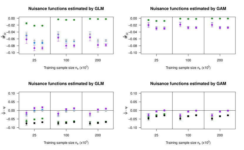
Finally, the results comparing the statistical performance of $\widehat{\mathbb{IF}}_{2,2,k}(\widehat{\Omega}^{emp})$, $\widehat{\mathbb{IF}}_{2,2,k}(\widehat{\Omega}^{ac})$ and $\widehat{\mathbb{IF}}_{2,2,k}(\widehat{g})$ (and also $\widehat{\psi}_{2,k}(\widehat{\Omega}^{emp})$, $\widehat{\psi}_{2,k}(\widehat{\Omega}^{ac})$ and $\widehat{\psi}_{2,k}(\widehat{g})$) are displayed in Figures 1 and 2 and Tables 1 to 4. We summarize our findings below:

  • On the upper-left panel of Figure 1, we compare $\widehat{\mathbb{IF}}_{2,2,k}(\Omega)$, $\widehat{\mathbb{IF}}_{2,2,k}(\widehat{\Omega}^{emp})$, $\widehat{\mathbb{IF}}_{2,2,k}(\widehat{\Omega}^{ac})$ and $\widehat{\mathbb{IF}}_{2,2,k}(\widehat{g})$ when the nuisance functions $b$ and $1/p$ are estimated by GLM. The error bars represent the inter-90%-quantiles out of 100 Monte Carlo repetitions. As expected, when the estimation sample size increases (from left to right within each column of every panel), the variability of the corresponding $\widehat{\mathbb{IF}}_{2,2,k}$ decreases, as the error bars become narrower. The Monte Carlo distributions of the oracle $\widehat{\mathbb{IF}}_{2,2,k}(\Omega)$ (grey dots and error bars) and $\widehat{\mathbb{IF}}_{2,2,k}(\widehat{\Omega}^{emp})$ (blue dots and error bars) are very close, as the error bars for these two statistics are almost on top of each other. However, the distribution of $\widehat{\mathbb{IF}}_{2,2,k}(\widehat{\Omega}^{ac})$ (purple dots and error bars) is quite different from that of the oracle $\widehat{\mathbb{IF}}_{2,2,k}(\Omega)$ and $\widehat{\mathbb{IF}}_{2,2,k}(\widehat{\Omega}^{emp})$. The difference between $\widehat{\mathbb{IF}}_{2,2,k}(\widehat{g})$ (green dots and error bars) and the other statistics is even more striking.

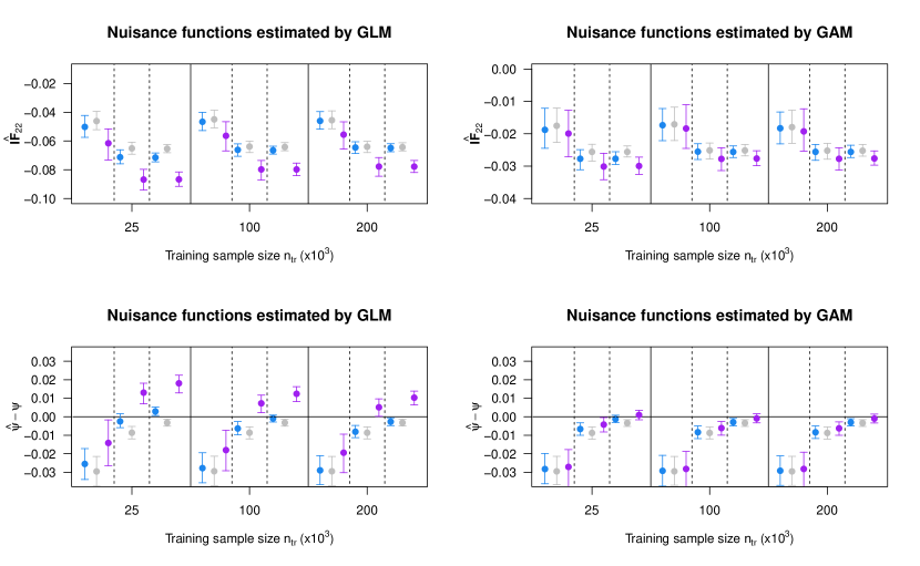
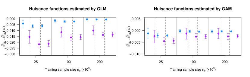
    On the upper-right panel of Figure 1, the nuisance functions $b$ and $1/p$ are estimated by GAM. The difference between $\widehat{\mathbb{IF}}_{2,2,k}(\widehat{g})$ and all the other statistics is obvious. But from this panel alone, it is hard to distinguish between $\widehat{\mathbb{IF}}_{2,2,k}(\Omega)$, $\widehat{\mathbb{IF}}_{2,2,k}(\widehat{\Omega}^{emp})$ and $\widehat{\mathbb{IF}}_{2,2,k}(\widehat{\Omega}^{ac})$. Therefore in Figure 2, we plot everything as in Figure 1, but discard the results of $\widehat{\mathbb{IF}}_{2,2,k}(\widehat{g})$. Thus Figure 2 is a zoom-in of Figure 1. From the upper-right panel of Figure 2, we can now clearly observe that the empirical distribution of $\widehat{\mathbb{IF}}_{2,2,k}(\widehat{\Omega}^{emp})$ (blue dots and error bars) is closer to the empirical distribution of $\widehat{\mathbb{IF}}_{2,2,k}(\Omega)$ (grey dots and error bars) than that of $\widehat{\mathbb{IF}}_{2,2,k}(\widehat{\Omega}^{ac})$ (purple dots and error bars). To further highlight this observation, we also display the empirical distributions of $\widehat{\mathbb{IF}}_{2,2,k}(\widehat{\Omega}^{emp})-\widehat{\mathbb{IF}}_{2,2,k}(\Omega)$ and $\widehat{\mathbb{IF}}_{2,2,k}(\widehat{\Omega}^{ac})-\widehat{\mathbb{IF}}_{2,2,k}(\Omega)$ in Figure 3 and it is apparent that the empirical distribution of $\widehat{\mathbb{IF}}_{2,2,k}(\widehat{\Omega}^{emp})-\widehat{\mathbb{IF}}_{2,2,k}(\Omega)$ is much closer to 0.

    All the above observations from the upper panels of Figures 1 and 2 can also be made from Tables 1 and 3, in which we display the Monte Carlo averages and standard deviations of different versions of $\widehat{\mathbb{IF}}_{2,2,k}$ across different training and estimation sample sizes. For example, the Monte Carlo averages of $\widehat{\mathbb{IF}}_{2,2,k}(\widehat{\Omega}^{emp})$ are always closer to the corresponding Monte Carlo averages of the oracle $\widehat{\mathbb{IF}}_{2,2,k}(\Omega)$ than those of $\widehat{\mathbb{IF}}_{2,2,k}(\widehat{\Omega}^{ac})$ in both Table 1 (nuisance functions estimated by GLM) and Table 3 (nuisance functions estimated by GAM); in addition the Monte Carlo standard deviations of $\widehat{\mathbb{IF}}_{2,2,k}(\widehat{\Omega}^{emp})$ are always smaller than those of $\widehat{\mathbb{IF}}_{2,2,k}(\widehat{\Omega}^{ac})$.

  • On the lower panels of Figure 1, we compare the bias of estimating $\psi$ before ($\widehat{\psi}_{1}$, black dots and error bars) or after bias correction ($\widehat{\psi}_{2,k}(\Omega)=\widehat{\psi}_{1}+\widehat{\mathbb{IF}}_{2,2,k}(\Omega)$ grey dots and error bars, $\widehat{\psi}_{2,k}(\widehat{\Omega}^{emp})=\widehat{\psi}_{1}+\widehat{\mathbb{IF}}_{2,2,k}(\widehat{\Omega}^{emp})$ blue dots and error bars, $\widehat{\psi}_{2,k}(\widehat{\Omega}^{ac})=\widehat{\psi}_{1}+\widehat{\mathbb{IF}}_{2,2,k}(\widehat{\Omega}^{ac})$ purple dots and error bars and $\widehat{\psi}_{2,k}(\widehat{g})=\widehat{\psi}_{1}+\widehat{\mathbb{IF}}_{2,2,k}(\widehat{g})$ green dots and error bars). In particular, $\widehat{\mathbb{IF}}_{2,2,k}(\widehat{g})$ corrects little bias, as the distribution of $\widehat{\psi}_{2,k}(\widehat{g})-\psi(\theta)$ is very close to the distribution of $\widehat{\psi}_{1}-\psi(\theta)$ across different estimation and training sample sizes, regardless whether the nuisance parameters are estimated by GLM (lower-left) or GAM (lower-right).

    From the lower-left panel of Figure 1, we observe that after corrected by $\widehat{\mathbb{IF}}_{2,2,k}(\Omega)$ (grey dots and error bars) or $\widehat{\mathbb{IF}}_{2,2,k}(\widehat{\Omega}^{emp})$ (blue dots and error bars), the biases of estimating $\psi$ are much closer to zero than using $\widehat{\psi}_{1}$ without any bias correction (black dots and error bars) or even using $\widehat{\psi}_{2,k}(\widehat{\Omega}^{ac})$ with bias corrected by $\widehat{\mathbb{IF}}_{2,2,k}(\widehat{\Omega}^{ac})$ (purple dots and error bars). From the lower-right panel of Figure 1, it is hard to distinguish the bias of $\widehat{\psi}_{2,k}(\widehat{\Omega}^{ac})$ from that of $\widehat{\psi}_{2,k}(\Omega)$ or $\widehat{\psi}_{2,k}(\widehat{\Omega}^{emp})$. Instead, we can examine the lower-right panel of Figure 2 in which the results of $\widehat{\psi}_{2,k}(\widehat{g})$ are discarded. Now we are able to observe that $\widehat{\psi}_{2,k}(\widehat{\Omega}^{emp})$ is still closer to $\widehat{\psi}_{2,k}(\Omega)$ than $\widehat{\psi}_{2,k}(\widehat{\Omega}^{ac})$, in particular as the training sample size increases. As displayed in Table 2, $\widehat{\psi}_{2,k}(\widehat{\Omega}^{ac})$ has smaller bias (for estimating $\psi(\theta)$) than $\widehat{\psi}_{2,k}(\widehat{\Omega}^{emp})$ or even the oracle estimator $\widehat{\psi}_{2,k}(\Omega)$. However, one should compare $\widehat{\psi}_{2,k}(\widehat{\Omega}^{ac})$ and $\widehat{\psi}_{2,k}(\widehat{\Omega}^{emp})$ to the oracle $\widehat{\psi}_{2,k}(\Omega)$ instead, because there is no theoretical reason for $\widehat{\psi}_{2,k}(\widehat{\Omega}^{ac})$ to have smaller bias than $\widehat{\psi}_{2,k}(\Omega)$. Therefore the bias of $\widehat{\psi}_{2,k}(\widehat{\Omega}^{ac})$ will be greater than that of $\widehat{\psi}_{2,k}(\Omega)$ for other simulation parameters.

    All the above observations made from the lower panels of Figures 1 and 2 can also be made from Tables 2 and 4, in which we display the Monte Carlo averages and standard deviations of different versions of $\widehat{\psi}_{2,k}$ across different training and estimation sample sizes. For example, we observe that the Monte Carlo averages of $\widehat{\psi}_{2,k}(\widehat{\Omega}^{emp})-\psi(\theta)$ are generally closer to those of $\widehat{\psi}_{2,k}(\Omega)-\psi(\theta)$ than those of $\widehat{\psi}_{2,k}(\widehat{\Omega}^{ac})-\psi(\theta)$; and the Monte Carlo standard deviations of $\widehat{\psi}_{2,k}(\widehat{\Omega}^{emp})-\psi(\theta)$ are also smaller than those of $\widehat{\psi}_{2,k}(\widehat{\Omega}^{ac})-\psi(\theta)$.

    Similarly, the observations made from Figure 3 can be read from Tables 5 and 6: Obviously the distribution of $\widehat{\mathbb{IF}}_{2,2,k}(\widehat{\Omega}^{emp})-\widehat{\mathbb{IF}}_{2,2,k}(\Omega)$ is much closer to 0 than that of $\widehat{\mathbb{IF}}_{2,2,k}(\widehat{\Omega}^{ac})-\widehat{\mathbb{IF}}_{2,2,k}(\Omega)$.

In summary, in the above simulation in which $g$ is very rough, $\widehat{\mathbb{IF}}_{2,2,k}(\widehat{\Omega}^{emp})$ (and also $\widehat{\psi}_{2,k}(\widehat{\Omega}^{emp})$) has better finite sample statistical performance and is relatively more efficient to compute than $\widehat{\mathbb{IF}}_{2,2,k}(\widehat{\Omega}^{ac})$ and $\widehat{\mathbb{IF}}_{2,2,k}(\widehat{g})$.

5 Literature overview and discussions

5.1 Literature overview

We now provide a literature overview of several other works that aim at achieving $\sqrt{n}$-consistent estimation under relaxed conditions for the class of functionals considered in this paper. For instance, the use of HOIF for bias correction has been considered in a series of papers (Tchetgen Tchetgen et al., 2008; Robins et al., 2008; Díaz, Carone and van der Laan, 2016; Carone, Díaz and van der Laan, 2018; Robins et al., 2017; Liu et al., 2021; Yu and Wang, 2020) but they all require either knowing the density of the covariates or estimating the density at a sufficiently fast rate. To the best of our knowledge, Newey and Robins (2018) is the first paper demonstrating the existence of $\sqrt{n}$-consistent estimators under minimal conditions of Robins et al. (2009b) for a subclass of the functionals considered in our paper, without using the HOIF machinery. However, that subclass does not include the mean of a response $Y$ under MAR or the average treatment effect under ignorable treatment assignment, except for the corner cases in which $\beta_{b}$ is much greater than $\beta_{p}$. Hirshberg and Wager (2021), Armstrong and Kolesár (2021), and Kennedy (2020) also obtained $\sqrt{n}$-consistent estimators for the ATE, but only for the aforementioned corner case. Therefore the empirical HOIF U-statistic estimator of diverging order proposed in this paper remains the only known $\sqrt{n}$-consistent estimator under (all) the minimal conditions of Robins et al. (2009b).

Liu, Mukherjee and Robins (2023) demonstrated another application of empirical HOIF estimators. The empirical HOIF estimators were used to construct a test of the hypothesis that $\widehat{\psi}_{1}$ based on the first-order influence function is a smaller order than its standard error (Liu, Mukherjee and Robins, 2020). It follows that when the test rejects, one can conclude that a nominal $(1-\alpha)\times 100\%$ large-sample Wald confidence interval centered around $\widehat{\psi}_{1}$ has an actual coverage less than $(1-\alpha)\times 100\%$.

5.2 Discussions

We have shown that for $\sqrt{n}$-estimable parameters the asymptotic properties of our new empirical HOIF estimators are identical to those of the HOIF estimators of Robins et al. (2008, 2017), yet eliminate the need to construct multivariate density estimates. In particular the new estimators are semiparametric efficient under minimal conditions of Robins et al. (2009b). We end our paper by pointing out several research directions:

  • It is interesting to generalize the theory of HOIFs developed in Robins et al. (2008, 2017) and of empirical HOIFs developed in our paper to other causal parameters or more complicated scenario, such as those in Tchetgen Tchetgen and Shpitser (2012); Bhattacharya, Nabi and Shpitser (2022); Cui et al. (2023). Liu, Mukherjee and Robins (2023) derive the HOIFs for the mean of a response $Y$ under MNAR under the so-called proximal causal inference framework (Cui et al., 2020), which can be used to improve on the first order influence estimator under that framework. Kennedy et al. (2022) used 2nd HOIFs to estimate the Conditional Average Treatment Effect (CATE) as a function of the covariates $X$ under ignorability. However their estimator did not achieve the minimax rate even when the CATE function was very smooth except when $g$ was also very smooth, because the order of the HOIF $U$-statistic estimator was not allowed to increase with sample size.

  • Another interesting and important open problem is to investigate if it is possible to estimate average treatment effect or equivalently the mean of a response $Y$ under MAR under the minimal conditions of Robins et al. (2009b) without using U-statistics of diverging order, e.g. using procedures similar to those in Newey and Robins (2018) and Kennedy (2020). We expect this to be not possible but we do not have a proof.

Refer to caption
Figure 1: Results of simulation experiment. The upper panels compare $\widehat{\mathbb{IF}}_{2,2,k}(\Omega)$, $\widehat{\mathbb{IF}}_{2,2,k}(\widehat{\Omega}^{emp})$, $\widehat{\mathbb{IF}}_{2,2,k}(\widehat{\Omega}^{ac})$ and $\widehat{\mathbb{IF}}_{2,2,k}(\widehat{g})$. Color code: black – $\widehat{\psi}_{1}-\psi(\theta)$; grey – $\widehat{\mathbb{IF}}_{2,2,k}(\Omega)$; blue – $\widehat{\mathbb{IF}}_{2,2,k}(\widehat{\Omega}^{emp})$; purple – $\widehat{\mathbb{IF}}_{2,2,k}(\widehat{\Omega}^{ac})$; green – $\widehat{\mathbb{IF}}_{2,2,k}(\widehat{g})$. The lower panels compare the estimators before and after being corrected by different versions of $\widehat{\mathbb{IF}}_{2,2,k}$, i.e. $\widehat{\psi}_{2,k}(\Omega)=\widehat{\psi}_{1}+\widehat{\mathbb{IF}}_{2,2,k}(\Omega)$, $\widehat{\psi}_{2,k}(\widehat{\Omega}^{emp})=\widehat{\psi}_{1}+\widehat{\mathbb{IF}}_{2,2,k}(\widehat{\Omega}^{emp})$, $\widehat{\psi}_{2,k}(\widehat{\Omega}^{ac})=\widehat{\psi}_{1}+\widehat{\mathbb{IF}}_{2,2,k}(\widehat{\Omega}^{ac})$, and $\widehat{\psi}_{2,k}(\widehat{g})=\widehat{\psi}_{1}+\widehat{\mathbb{IF}}_{2,2,k}(\widehat{g})$. Color code: black – $\widehat{\psi}_{1}-\psi(\theta)$; grey – $\widehat{\psi}_{2,k}(\Omega)-\psi(\theta)$; blue – $\widehat{\psi}_{2,k}(\widehat{\Omega}^{emp})-\psi(\theta)$; purple – $\widehat{\psi}_{2,k}(\widehat{\Omega}^{ac})-\psi(\theta)$; green – $\widehat{\psi}_{2,k}(\widehat{g})-\psi(\theta)$. In the panels on the left, the nuisance functions $b$ and $1/p$ are estimated by GLMs whereas in panels on the right, they are estimated by GAMs. The dots in each plot are the Monte Carlo averages across 100 simulated datasets. The error bars in each plot correspond to the 10% and 90% percentiles out of 100 Monte Carlo simulations. Within each column of any panel, from left to right we display the simulation results for estimation sample sizes $n=25000,100000,200000$.
Refer to caption
Figure 2: Results of simulation experiment. The color codes are the same as in Figure 1, except that the simulations for $\widehat{\mathbb{IF}}_{2,2,k}(\widehat{g})$ are removed from the upper panels and the simulations for $\widehat{\psi}_{1}-\psi(\theta)$ and $\widehat{\psi}_{2,k}(\widehat{g})-\psi(\theta)$ are removed from the lower panels. Within each column of any panel, from left to right we display the simulation results for estimation sample sizes $n=25000,100000,200000$.
Refer to caption
Figure 3: Results of simulation experiment. The color codes are the same as in Figure 1, except that only $\widehat{\mathbb{IF}}_{2,2,k}(\widehat{\Omega}^{emp})-\widehat{\mathbb{IF}}_{2,2,k}(\Omega)$ and $\widehat{\mathbb{IF}}_{2,2,k}(\widehat{\Omega}^{ac})-\widehat{\mathbb{IF}}_{2,2,k}(\Omega)$ are displayed to highlight the observation that $\widehat{\mathbb{IF}}_{2,2,k}(\widehat{\Omega}^{emp})$ is closer to the oracle $\widehat{\mathbb{IF}}_{2,2,k}(\Omega)$ than $\widehat{\mathbb{IF}}_{2,2,k}(\widehat{\Omega}^{ac})$. Within each column of any panel, from left to right we display the simulation results for estimation sample sizes $n=25000,100000,200000$.
$n_{tr}$ $n$ $\widehat{\mathbb{IF}}_{2,2,k}(\Omega)$ $\widehat{\mathbb{IF}}_{2,2,k}(\widehat{\Omega}^{emp})$ $\widehat{\mathbb{IF}}_{2,2,k}(\widehat{\Omega}^{ac})$ $\widehat{\mathbb{IF}}_{2,2,k}(\widehat{g})$
25,000 25,000 -4.62 (0.489) -5.02 (0.605) -6.16 (0.908) -1.48 (0.197)
100,000 25,000 -4.50 (0.481) -4.67 (0.496) -5.64 (0.801) -0.303 (0.0408)
200,000 25,000 -4.56 (0.480) -4.60 (0.483) -5.56 (0.749) -0.148 (0.0197)
25,000 100,000 -6.51 (0.318) -7.13 (0.373) -8.68 (0.584) -2.15 (0.116)
100,000 100,000 -6.39 (0.306) -6.62 (0.317) -7.98 (0.514) -0.450 (0.0233)
200,000 100,000 -6.40 (0.307) -6.45 (0.311) -7.78 (0.490) -0.217 (0.0113)
25,000 200,000 -6.54 (0.213) -7.15 (0.251) -8.67 (0.418) -2.15 (0.0804)
100,000 200,000 -6.42 (0.205) -6.65 (0.209) -7.98 (0.365) -0.452 (0.0158)
200,000 200,000 -6.43 (0.206) -6.48 (0.211) -7.78 (0.342) -0.218 (0.00761)
Table 1: Results of simulation experiment (nuisance functions estimated by GLMs): Column 1: training sample size; column 2: estimation sample size; columns 3 - 7: Monte Carlo means (and standard deviations) of $10^{-2}\times\widehat{\mathbb{IF}}_{2,2,k}(\Omega)$, $10^{-2}\times\widehat{\mathbb{IF}}_{2,2,k}(\widehat{\Omega}^{emp})$, $10^{-2}\times\widehat{\mathbb{IF}}_{2,2,k}(\widehat{\Omega}^{ac})$ and $10^{-2}\times\widehat{\mathbb{IF}}_{2,2,k}(\widehat{g})$.
$n_{tr}$ $n$ $\widehat{\psi}_{1}-\psi(\theta)$ $\widehat{\psi}_{2,k}(\Omega)-\psi(\theta)$ $\widehat{\psi}_{2,k}(\widehat{\Omega}^{emp})-\psi(\theta)$ $\widehat{\psi}_{2,k}(\widehat{\Omega}^{ac})-\psi(\theta)$ $\widehat{\psi}_{2,k}(\widehat{g})-\psi(\theta)$
25,000 25,000 -7.57 (0.759) -2.96 (0.662) -2.55 (0.718) -1.42 (0.944) -6.10 (0.719)
100,000 25,000 -7.44 (0.756) -2.95 (0.662) -2.78 (0.646) -1.80 (0.868) -7.14 (0.744)
200,000 25,000 -7.50 (0.755) -2.95 (0.662) -2.90 (0.662) -1.95 (0.831) -7.36 (0.749)
25,000 100,000 -7.38 (0.353) -0.866 (0.251) -0.252 (0.289) 1.30 (0.453) -5.23 (0.288)
100,000 100,000 -7.25 (0.346) -0.865 (0.248) -0.636 (0.258) 0.725 (0.398) -6.81 (0.322)
200,000 100,000 -7.27 (0.347) -0.866 (0.249) -0.811 (0.255) 0.512 (0.378) -7.05 (0.339)
25,000 200,000 -6.86 (0.225) -0.322 (0.153) 0.288 (0.183) 1.81 (0.356) -4.71 (0.184)
100,000 200,000 -6.74 (0.221) -0.321 (0.152) 0.0900 (0.154) 1.24 (0.306) -6.29 (0.211)
200,000 200,000 -6.75 (0.221) -0.321 (0.152) 0.0267 (0.157) 1.03 (0.284) -6.53 (0.217)
Table 2: Results of simulation experiment (nuisance functions estimated by GLMs): Column 1: training sample size; column 2: estimation sample size; columns 3 - 7: Monte Carlo means (and standard deviations) of $10^{-2}\times(\widehat{\psi}_{1}-\psi(\theta))$, $10^{-2}\times(\widehat{\psi}_{2,k}(\Omega)-\psi(\theta))$, $10^{-2}\times(\widehat{\psi}_{2,k}(\widehat{\Omega}^{emp})-\psi(\theta))$, $10^{-2}\times(\widehat{\psi}_{2,k}(\widehat{\Omega}^{ac})-\psi(\theta))$ and $10^{-2}\times(\widehat{\psi}_{2,k}(\widehat{g})-\psi(\theta))$.
$n_{tr}$ $n$ $\widehat{\mathbb{IF}}_{2,2,k}(\Omega)$ $\widehat{\mathbb{IF}}_{2,2,k}(\widehat{\Omega}^{emp})$ $\widehat{\mathbb{IF}}_{2,2,k}(\widehat{\Omega}^{ac})$ $\widehat{\mathbb{IF}}_{2,2,k}(\widehat{g})$
25,000 25,000 -1.75 (0.489) -1.88 (0.494) -1.99 (0.616) -0.500 (0.151)
100,000 25,000 -1.71 (0.481) -1.73 (0.411) -1.84 (0.551) -0.101 (0.0321)
200,000 25,000 -1.79 (0.480) -1.83 (0.418) -1.93 (0.527) -0.0497 (0.0154)
25,000 100,000 -2.56 (0.202) -2.77 (0.231) -3.01 (0.310) -0.772 (0.0718)
100,000 100,000 -2.51 (0.198) -2.55 (0.201) -2.78 (0.275) -0.162 (0.0152)
200,000 100,000 -2.52 (0.196) -2.56 (0.198) -2.77 (0.265) -0.0768 (0.00724)
25,000 200,000 -2.56 (0.135) -2.77 (0.155) -3.00 (0.211) -0.765 (0.0469)
100,000 200,000 -2.52 (0.134) -2.56 (0.139) -2.76 (0.185) -0.162 (0.00983)
200,000 200,000 -2.52 (0.135) -2.56 (0.138) -2.76 (0.177) -0.0768 (0.00470)
Table 3: Results of simulation experiment (nuisance functions estimated by GAMs): Column 1: training sample size; column 2: estimation sample size; columns 3 - 6: Monte Carlo means (and standard deviations) of $10^{-2}\times\widehat{\mathbb{IF}}_{2,2,k}(\Omega)$, $10^{-2}\times\widehat{\mathbb{IF}}_{2,2,k}(\widehat{\Omega}^{emp})$, $10^{-2}\times\widehat{\mathbb{IF}}_{2,2,k}(\widehat{\Omega}^{ac})$ and $10^{-2}\times\widehat{\mathbb{IF}}_{2,2,k}(\widehat{g})$.
$n_{tr}$ $n$ $\widehat{\psi}_{1}-\psi(\theta)$ $\widehat{\psi}_{2,k}(\Omega)-\psi(\theta)$ $\widehat{\psi}_{2,k}(\widehat{\Omega}^{emp})-\psi(\theta)$ $\widehat{\psi}_{2,k}(\widehat{\Omega}^{ac})-\psi(\theta)$ $\widehat{\psi}_{2,k}(\widehat{g})-\psi(\theta)$
25,000 25,000 -4.71 (0.709) -2.95 (0.648) -2.83 (0.691) -2.71 (0.767) -4.21 (0.670)
100,000 25,000 -4.66 (0.708) -2.95 (0.648) -2.93 (0.654) -2.82 (0.738) -4.56 (0.697)
200,000 25,000 -4.75 (0.705) -2.95 (0.649) -2.92 (0.656) -2.83 (0.723) -4.79 (0.700)
25,000 100,000 -3.44 (0.304) -0.877 (0.242) -0.664 (0.264) -0.424 (0.304) -2.66 (0.269)
100,000 100,000 -3.39 (0.300) -0.876 (0.240) -0.838 (0.242) -0.614 (0.281) -3.23 (0.292)
200,000 100,000 -3.40 (0.299) -0.877 (0.240) -0.841 (0.242) -0.626 (0.275) -3.32 (0.295)
25,000 200,000 -2.90 (0.167) -0.340 (0.151) -0.128 (0.159) 0.0961 (0.211) -2.13 (0.151)
100,000 200,000 -2.85 (0.164) -0.339 (0.151) -0.294 (0.151) -0.0901 (0.192) -2.69 (0.160)
200,000 200,000 -2.86 (0.165) -0.340 (0.151) -0.303 (0.153) -0.100 (0.184) -2.77 (0.163)
Table 4: Results of simulation experiment (nuisance functions estimated by GAMs): Column 1: training sample size; column 2: estimation sample size; columns 3 - 6: Monte Carlo means (and standard deviations) of $10^{-2}\times(\widehat{\psi}_{1}-\psi(\theta))$, $10^{-2}\times(\widehat{\psi}_{2,k}(\Omega)-\psi(\theta))$, $10^{-2}\times(\widehat{\psi}_{2,k}(\widehat{\Omega}^{emp})-\psi(\theta))$, $10^{-2}\times(\widehat{\psi}_{2,k}(\widehat{\Omega}^{ac})-\psi(\theta))$ and $10^{-2}\times(\widehat{\psi}_{2,k}(\widehat{g})-\psi(\theta))$.
$n_{tr}$ $n$ $\widehat{\mathbb{IF}}_{2,2,k}(\widehat{\Omega}^{emp})-\widehat{\mathbb{IF}}_{2,2,k}(\Omega)$ $\widehat{\mathbb{IF}}_{2,2,k}(\widehat{\Omega}^{ac})-\widehat{\mathbb{IF}}_{2,2,k}(\Omega)$
25,000 25,000 -4.06 (2.18) -15.41 (3.43)
100,000 25,000 -1.69 (0.865) -11.44 (2.89)
200,000 25,000 -0.491 (0.537) -10.04 (2.59)
25,000 100,000 -6.15 (1.12) -21.70 (1.88)
100,000 100,000 -2.29 (0.514) -15.90 (1.56)
200,000 100,000 -0.545 (0.340) -13.78 (1.42)
25,000 200,000 -6.11 (0.835) -21.31 (1.52)
100,000 200,000 -2.31 (0.356) -15.62 (1.26)
200,000 200,000 -0.540 (0.224) -13.52 (1.13)
Table 5: Results of simulation experiment (nuisance functions estimated by GLMs): Column 1: training sample size; column 2: estimation sample size; columns 3 - 4: Monte Carlo means (and standard deviations) of $10^{-3}\times(\widehat{\mathbb{IF}}_{2,2,k}(\widehat{\Omega}^{emp})-\widehat{\mathbb{IF}}_{2,2,k}(\Omega))$ and $10^{-3}\times(\widehat{\mathbb{IF}}_{2,2,k}(\widehat{\Omega}^{ac})-\widehat{\mathbb{IF}}_{2,2,k}(\Omega))$.
$n_{tr}$ $n$ $\widehat{\mathbb{IF}}_{2,2,k}(\widehat{\Omega}^{emp})-\widehat{\mathbb{IF}}_{2,2,k}(\Omega)$ $\widehat{\mathbb{IF}}_{2,2,k}(\widehat{\Omega}^{ac})-\widehat{\mathbb{IF}}_{2,2,k}(\Omega)$
25,000 25,000 -1.25 (1.63) -2.40 (2.01)
100,000 25,000 -0.269 (0.633) -1.30 (1.68)
200,000 25,000 -0.344 (0.472) -1.32 (1.50)
25,000 100,000 -2.12 (0.768) -4.53 (0.902)
100,000 100,000 -0.381 (0.326) -2.62 (0.719)
200,000 100,000 -0.366 (0.232) -2.51 (0.657)
25,000 200,000 -2.12 (0.497) -4.36 (0.711)
100,000 200,000 -0.450 (0.231) -2.49 (0.567)
200,000 200,000 -0.374 (0.152) -2.40 (0.501)
Table 6: Results of simulation experiment (nuisance functions estimated by GAMs): Column 1: training sample size; column 2: estimation sample size; columns 3 - 4: Monte Carlo means (and standard deviations) of $10^{-3}\times(\widehat{\mathbb{IF}}_{2,2,k}(\widehat{\Omega}^{emp})-\widehat{\mathbb{IF}}_{2,2,k}(\Omega))$ and $10^{-3}\times(\widehat{\mathbb{IF}}_{2,2,k}(\widehat{\Omega}^{ac})-\widehat{\mathbb{IF}}_{2,2,k}(\Omega))$.

6 Proofs

Proof of Theorem 2 and 3.

We divide our proof into bias and variance computations respectively. Throughout we assume $I(h_{1}(W)\leq 0)=1$ almost surely. The case $I(h_{1}(W)\geq 0$ requires obvious sign changes in various place.

6.1 Bias bound

The proof for $\mathrm{EB}_{m,k}^{ac}(\theta)$ has appeared in Robins et al. (2008), hence omitted. Throughout the proof $\widehat{\Omega}$ stands for $\widehat{\Omega}^{emp}$. By the same analysis as in Robins et al. (2008),

$$\mathrm{EB}_{m,k}^{emp}\left(\theta\right)=(-1)^{m}\mathbb{E}_{\theta}[H_{1}(P-\widehat{P})\bar{Z}_{k}^{\top}]\Omega^{-1}\left[\left\{\Omega-\widehat{\Omega}\right\}\widehat{\Omega}^{-1}\right]^{m-1}\mathbb{E}_{\theta}[\bar{Z}_{k}H_{1}(B-\widehat{B})].$$

We next show that under the assumptions of Theorem 3

$$\left|\mathrm{EB}_{m,k}^{emp}\left(\theta\right)\right|=O\left(\|\widehat{\Omega}-\Omega\|_{op}^{m-1}\left\{\mathbb{E}_{\theta}[(B-\widehat{B})^{2}]\mathbb{E}_{\theta}[(P-\widehat{P})^{2}]\right\}^{1/2}\right),$$

where $\|\cdot\|_{op}$ denotes the operator norm of a matrix.

Now let $\widehat{1}$ denote the indicator function for the event that $\lambda_{\max}(\widehat{\Omega}^{-1})\leq C^{-1}$. In the rest of the proof we take $C>0$ large enough such that $\lambda_{\max}({\Omega}^{-1})\leq C^{-1}$ as well (note that this is allowed by Condition B assumed in the statement of the theorem).

By Cauchy-Schwarz inequality,

$$\left|\mathrm{EB}_{m,k}^{emp}(\theta)\right|\leq\left\|\mathbb{E}_{\theta}[H_{1}(P-\widehat{P})\bar{Z}_{k}^{\top}]\Omega^{-1/2}\right\|\left\|\Omega^{-1/2}\left[\left\{\Omega-\widehat{\Omega}\right\}\widehat{\Omega}^{-1}\right]^{m-1}\mathbb{E}_{\theta}[\bar{Z}_{k}H_{1}(B-\widehat{B})]\right\|.$$

Note that $\left\|\mathbb{E}_{\theta}[H_{1}(P-\widehat{P})\bar{Z}_{k}^{\top}]\Omega^{-1/2}\right\|^{2}$ is the second moment of the linear projection of $-(P-\widehat{P})$ on $\bar{Z}_{k}$ under $g$, so that

$$\left\|\mathbb{E}_{\theta}[H_{1}(P-\widehat{P})\bar{Z}_{k}^{\top}]\Omega^{-1/2}\right\|\leq\left\{\mathbb{E}_{\theta}[(P-\widehat{P})^{2}]\right\}^{1/2}.$$

Also, note that for $\Sigma=\Omega^{-1/2}\left[\left\{\Omega-\widehat{\Omega}\right\}\widehat{\Omega}^{-1}\right]^{m-1}$, in the positive semi-definite sense

$\displaystyle\widehat{1}\Sigma^{\top}\Sigma$ $\displaystyle=\widehat{1}\left[\widehat{\Omega}^{-1}\left\{\Omega-\widehat{\Omega}\right\}\right]^{m-1}\Omega^{-1}\left[\left\{\Omega-\widehat{\Omega}\right\}\widehat{\Omega}^{-1}\right]^{m-1}$
$\displaystyle\leq\widehat{1}C^{-1}\left[\widehat{\Omega}^{-1}\left\{\Omega-\widehat{\Omega}\right\}\right]^{m-1}\left[\left\{\Omega-\widehat{\Omega}\right\}\widehat{\Omega}^{-1}\right]^{m-1}$
$\displaystyle=\widehat{1}C^{-1}\left[\widehat{\Omega}^{-1}\left\{\Omega-\widehat{\Omega}\right\}\right]^{m-2}\widehat{\Omega}^{-1}\left\{\Omega-\widehat{\Omega}\right\}^{2}\widehat{\Omega}^{-1}\left[\left\{\Omega-\widehat{\Omega}\right\}\widehat{\Omega}^{-1}\right]^{m-2}$
$\displaystyle\leq\left\|\Omega-\widehat{\Omega}\right\|_{op}^{2}\widehat{1}C^{-1}\left[\widehat{\Omega}^{-1}\left\{\Omega-\widehat{\Omega}\right\}\right]^{m-2}\widehat{\Omega}^{-2}\left[\left\{\Omega-\widehat{\Omega}\right\}\widehat{\Omega}^{-1}\right]^{m-2}$
$\displaystyle\leq\left\|\Omega-\widehat{\Omega}\right\|_{op}^{2}\widehat{1}C^{-3}\left[\widehat{\Omega}^{-1}\left\{\Omega-\widehat{\Omega}\right\}\right]^{m-2}\left[\left\{\Omega-\widehat{\Omega}\right\}\widehat{\Omega}^{-1}\right]^{m-2}.$

Repeating this argument (i.e. by induction) we have

$$\widehat{1}\Sigma^{\top}\Sigma\leq\widehat{1}\left\|\Omega-\widehat{\Omega}\right\|_{op}^{2(m-1)}C^{-2(m-1)-1}I.$$

Next, since $I\leq\Omega^{-1}C$ in the p.s.d. sense we have

$$\widehat{1}\Sigma^{\top}\Sigma\leq\widehat{1}\left\|\Omega-\widehat{\Omega}\right\|_{op}^{2(m-1)}C^{-2(m-1)}\Omega^{-1}.$$

It then follows that

$\displaystyle\widehat{1}\left\|\Omega^{-1/2}\left[\left\{\Omega-\widehat{\Omega}\right\}\widehat{\Omega}^{-1}\right]^{m-1}\mathbb{E}_{\theta}[\bar{Z}_{k}H_{1}(B-\widehat{B})]\right\|^{2}$
$\displaystyle=\widehat{1}\left\|H_{1}\mathbb{E}_{\theta}[\bar{Z}_{k}H_{1}(B-\widehat{B})]\right\|^{2}=\widehat{1}\mathbb{E}_{\theta}[H_{1}(B-\widehat{B})\bar{Z}_{k}^{\top}]H^{\top}H\mathbb{E}_{\theta}[\bar{Z}_{k}H_{1}(B-\widehat{B})]$
$\displaystyle\leq\widehat{1}\left\|\Omega-\widehat{\Omega}\right\|_{op}^{2(m-1)}C^{-2(m-1)}\mathbb{E}_{\theta}[H_{1}(B-\widehat{B})\bar{Z}_{k}^{\top}]\Omega^{-1}\mathbb{E}_{\theta}[\bar{Z}_{k}H_{1}(B-\widehat{B})].$
$\displaystyle\leq\widehat{1}\left\|\Omega-\widehat{\Omega}\right\|_{op}^{2(m-1)}C^{-2(m-1)}\mathbb{E}_{\theta}[(B-\widehat{B})^{2}],$

where the last inequality follows by $\mathbb{E}_{\theta}[H_{1}(B-\widehat{B})\bar{Z}_{k}^{\top}]\Omega^{-1}\mathbb{E}_{\theta}[\bar{Z}_{k}H_{1}(B-\widehat{B})]$ being the expected square of the projection of $B-\widehat{B}$ on $\bar{Z}_{k}$ under $g$. Therefore we have

$\displaystyle\widehat{1}\left|\mathrm{EB}_{m,k}^{emp}\right|$ $\displaystyle\leq\widehat{1}\left\|\Omega-\widehat{\Omega}\right\|_{op}^{m-1}C^{-(m-1)}\left\{\mathbb{E}_{\theta}[(B-\widehat{B})^{2}]\mathbb{E}_{\theta}[(P-\widehat{P})^{2}]\right\}^{1/2}.$

This completes the bound for the bias.

6.2 Variance bound

The strategy for the variance bound proof applies to both the empirical HOIF estimators and the HOIF estimators based on density estimation. In this section, we only prove the variance bound for generic $\widehat{\Omega}$, hence including both $\widehat{\Omega}^{emp}$ and $\widehat{\Omega}^{ac}$.

In the proof, the constant $C$, independent of the sample size, will change from line to line. In this section we are agnostic to the specific forms of $\varepsilon_{\widehat{b}}$ and $\varepsilon_{\widehat{p}}$ except that they are bounded with $\mathbb{P}_{\theta}$-probability 1.

For convenience, we introduce the $j$-th order U-statistic operator $\mathbb{U}_{n}(h(O_{\overline{i}_{j}}))$, for any nonnegative integer $j$ and any function $h:\mathbb{R}^{j}\rightarrow\mathbb{R}$:

$\displaystyle\mathbb{U}_{n}(h(O_{\overline{i}_{j}}))\coloneqq\frac{(n-j)!}{n!}\sum_{1\leq i_{1}\neq i_{2}\neq\cdots\neq i_{j}\leq n}h(O_{\overline{i}_{j}}).$

To control the variance of $\widehat{\psi}_{m,k}$ we begin with the following variance bound of $\widehat{\mathbb{IF}}_{22}\equiv\mathbb{U}_{n}(\widehat{\mathrm{IF}}_{2,2,k,\overline{i}_{2}})$, whose proof is a straightforward application of Hoeffding decomposition.

Lemma 9.

Under the conditions of Theorem 2 or 3, there exists a positive constant $C$, depending only on $(\bar{z}_{k},p,\widehat{p},b,\widehat{b},g)$ such that

$$\begin{split}\mathrm{var}_{\theta}\left(\mathbb{U}_{n}(\widehat{\mathrm{IF}}_{2,2,k,\overline{i}_{2}})\right)&\leq\frac{C}{n}\left\{\frac{k}{n}+\mathbb{L}_{2,\widehat{b},k}^{2}+\mathbb{L}_{2,\widehat{p},k}^{2}\right\}.\end{split}$$ (6.1)
Proof.

By Hoeffding decomposition,

$\displaystyle\ -\left\{\mathbb{U}_{n}(\widehat{\mathrm{IF}}_{2,2,k,\overline{i}_{2}})-\mathbb{E}_{\theta}[\mathbb{U}_{n}(\widehat{\mathrm{IF}}_{2,2,k,\overline{i}_{2}})]\right\}$
$\displaystyle=$ $\displaystyle\ \underbrace{\frac{1}{n}\sum_{i=1}^{n}\mathbb{E}_{\theta}\left[\varepsilon_{\widehat{b}}\bar{z}_{k}(X)\right]^{\top}\widehat{\Omega}^{-1}\left\{\bar{z}_{k}(X_{i})\varepsilon_{\widehat{p},i}-\mathbb{E}_{\theta}\left[\varepsilon_{\widehat{p}}\bar{z}_{k}(X)\right]\right\}}_{T_{11}}$
$\displaystyle+\underbrace{\frac{1}{n}\sum_{i=1}^{n}\mathbb{E}_{\theta}\left[\varepsilon_{\widehat{p}}\bar{z}_{k}(X)\right]^{\top}\widehat{\Omega}^{-1}\left\{\bar{z}_{k}(X_{i})\varepsilon_{\widehat{b},i}-\mathbb{E}_{\theta}\left[\varepsilon_{\widehat{b}}\bar{z}_{k}(X)\right]\right\}}_{T_{12}}$
$\displaystyle+\underbrace{\frac{1}{n(n-1)}\sum_{1\leq i_{1}\neq i_{2}\leq n}\left\{\varepsilon_{\widehat{b},i_{1}}\bar{z}_{k}(X_{i_{1}})-\mathbb{E}_{\theta}\left[\varepsilon_{\widehat{b}}\bar{z}_{k}(X)\right]\right\}^{\top}\widehat{\Omega}^{-1}\left\{\bar{z}_{k}(X_{i_{2}})\varepsilon_{\widehat{p},i_{2}}-\mathbb{E}_{\theta}\left[\bar{z}_{k}(X)\varepsilon_{\widehat{p}}\right]\right\}}_{T_{2}}.$

Define $\widetilde{\Omega}\coloneqq\int\bar{z}_{k}(x)\bar{z}_{k}(x)f(x)dx$. Then under the assumptions (Condition B.2 and boundedness of $f$ and $|H_{1}|$) in our paper, there exists a universal constant $B^{\prime}>0$ such that $\frac{1}{B^{\prime}}\leq\lambda_{\min}(\widetilde{\Omega})\leq\lambda_{\max}(\widetilde{\Omega})\leq B^{\prime}$.

For the linear term $T_{11}$, we have

$\displaystyle\mathrm{var}_{\theta}[T_{11}]$ $\displaystyle\leq\frac{1}{n}\|\varepsilon_{\widehat{p}}^{2}\|_{\infty}\mathbb{E}_{\theta}\left[\varepsilon_{\widehat{b}}\bar{z}_{k}(X)\right]^{\top}\widehat{\Omega}^{-1}\mathbb{E}_{\theta}\left[\bar{z}_{k}(X)\bar{z}_{k}(X)^{\top}\right]\widehat{\Omega}^{-1}\mathbb{E}_{\theta}\left[\bar{z}_{k}(X)\varepsilon_{\widehat{b}}\right]$
$\displaystyle\leq\frac{1}{n}\|\varepsilon_{\widehat{p}}^{2}\|_{\infty}\mathbb{E}_{\theta}\left[\varepsilon_{\widehat{b}}\bar{z}_{k}(X)\right]^{\top}\Omega^{-1/2}\left(\Omega^{1/2}\widehat{\Omega}^{-1}\widetilde{\Omega}^{1/2}\right)^{2}\Omega^{-1/2}\mathbb{E}_{\theta}\left[\bar{z}_{k}(X)\varepsilon_{\widehat{b}}\right]$
$\displaystyle\leq\frac{1}{n}\|\varepsilon_{\widehat{p}}^{2}\|_{\infty}\mathbb{L}_{2,\widehat{b},k}^{2}$

where the last inequality follows from the definition of matrix operator norm. By symmetry,

$\displaystyle\mathrm{var}_{\theta}[T_{12}]\leq\frac{1}{n}\|\varepsilon_{\widehat{b}}^{2}\|_{\infty}\mathbb{L}_{2,\widehat{p},k}^{2}.$

For the second-order degenerate U-statistic term $T_{2}$, we have

$\displaystyle\mathrm{var}_{\theta}[T_{2}]$ $\displaystyle\leq\frac{1}{n(n-1)}\mathbb{E}_{\theta}\left[\varepsilon_{\widehat{b},1}^{2}\varepsilon_{\widehat{p},2}^{2}\left(\bar{z}_{k}(X_{1})^{\top}\widehat{\Omega}^{-1}\bar{z}_{k}(X_{2})\right)^{2}\right]$
$\displaystyle\leq\frac{C}{n^{2}}\|\varepsilon_{\widehat{b}}^{2}\varepsilon_{\widehat{p}}^{2}\|_{\infty}\mathbb{E}_{\theta}\left[\bar{z}_{k}(X)^{\top}\widehat{\Omega}^{-1}\widetilde{\Omega}\widehat{\Omega}^{-1}\bar{z}_{k}(X)\right]$
$\displaystyle\leq\frac{C}{n}\frac{k}{n}\|\varepsilon_{\widehat{b}}^{2}\varepsilon_{\widehat{p}}^{2}\|_{\infty}.$

Above the last inequality follows by Lemma 18.

Finally applying $\mathrm{var}_{\theta}[\mathbb{U}_{n}(\widehat{\mathrm{IF}}_{2,2,k,\overline{i}_{2}})]=\mathrm{var}_{\theta}[T_{11}+T_{12}]+\mathrm{var}_{\theta}[T_{2}]\leq 2\mathrm{var}_{\theta}[T_{11}]+2\mathrm{var}_{\theta}[T_{12}]+\mathrm{var}_{\theta}[T_{2}]$, we obtain

$$\mathrm{var}_{\theta}[\mathbb{U}_{n}(\widehat{\mathrm{IF}}_{2,2,k,\overline{i}_{2}})]\leq\frac{C}{n}\left\{\mathbb{L}_{2,\widehat{b},k}^{2}\|\varepsilon_{\widehat{p}}^{2}\|_{\infty}+\|\varepsilon_{\widehat{b}}^{2}\|_{\infty}\mathbb{L}_{2,\widehat{p},k}^{2}+\frac{k}{n}\|\varepsilon_{\widehat{b}}^{2}\varepsilon_{\widehat{p}}^{2}\|_{\infty}\right\}.$$


Next we compute the variance bound of $\widehat{\mathbb{IF}}_{33}\equiv\mathbb{U}_{n}(\widehat{\mathrm{IF}}_{3,3,k,\overline{i}_{3}})$. In particular, we have

Lemma 10.

Under the conditions of Theorem 2 or 3, there exists a positive constant $C$, depending only on $(\bar{z}_{k},p,\widehat{p},b,\widehat{b},g)$ such that

$$\begin{split}\mathrm{var}_{\theta}\left(\mathbb{U}_{n}(\widehat{\mathrm{IF}}_{3,3,k,\overline{i}_{3}})\right)&\leq\frac{C}{n}\left\{\begin{array}[]{c}\left(\dfrac{k}{n}\right)^{2}+\dfrac{k}{n}\left(\mathbb{L}_{2,\widehat{b},k}^{2}+\mathbb{L}_{2,\widehat{p},k}^{2}+\mathbb{L}_{2,\widehat{\Omega},k}^{2}\right)\\ +\left(\mathbb{L}_{2,\widehat{b},k}^{2}\mathbb{L}_{2,\widehat{\Omega},k}^{2}+\mathbb{L}_{2,\widehat{p},k}^{2}\mathbb{L}_{2,\widehat{\Omega},k}^{2}+\min\limits_{(\eta,\zeta):1/\eta+1/\zeta=1}\mathbb{L}_{\eta,\widehat{b},k}^{2}\mathbb{L}_{\zeta,\widehat{p},k}^{2}\right)\end{array}\right\}.\end{split}$$ (6.2)

The proof of Lemma 10 can be found in Appendix A.1.

For general $j>3$, we have the following result.

Lemma 11.

Under the conditions of Theorem 2 or 3, up to a universal constant depending only on $(\bar{z}_{k},p,\widehat{p},b,\widehat{b},g)$, we have

$$\begin{split}&\ \mathrm{var}_{\theta}\left(\mathbb{U}_{n}(\widehat{\mathrm{IF}}_{j,j,k,\overline{i}_{j}})\right)\\ \lesssim&\ \frac{j^{2}}{n}\mathbb{L}_{2,\widehat{\Omega},k}^{2(j-3)}\left(\mathbb{L}_{2,\widehat{b},k}^{2}\mathbb{L}_{2,\widehat{\Omega},k}^{2}+\mathbb{L}_{2,\widehat{p},k}^{2}\mathbb{L}_{2,\widehat{\Omega},k}^{2}+\min\limits_{(\eta,\zeta):1/\eta+1/\zeta=1}\mathbb{L}_{\eta,\widehat{b},k}^{2}\mathbb{L}_{\zeta,\widehat{p},k}^{2}\right)\\ &+\frac{1}{n}\sum_{\ell=2}^{j-1}j^{2\ell}\left(\frac{C^{\prime}k}{n}\right)^{\ell-1}\mathbb{L}_{2,\widehat{\Omega},k}^{2(j-\ell-2)\vee 0}\left(\begin{array}[]{c}\mathbb{L}_{2,\widehat{\Omega},k}^{4}+\mathbb{L}_{2,\widehat{b},k}^{2}\mathbb{L}_{2,\widehat{\Omega},k}^{2}+\mathbb{L}_{2,\widehat{p},k}^{2}\mathbb{L}_{2,\widehat{\Omega},k}^{2}\\ +\min\limits_{(\eta,\zeta):1/\eta+1/\zeta=1}\mathbb{L}_{\eta,\widehat{b},k}^{2}\mathbb{L}_{\zeta,\widehat{p},k}^{2}\end{array}\right)+\frac{j^{2j}}{n}\left(\frac{C^{\prime}k}{n}\right)^{j-1}.\end{split}$$ (6.3)

The proof of this lemma involves quite tedious calculations so we defer it to Appendix A.2.

Then combining Lemma 9, 10, 11 and the following inequalities:

$$\mathrm{var}_{\theta}\left(\sum_{\ell=1}^{j}G_{\ell}\right)\leq\sum_{\ell=1}^{j}2^{\ell}\mathrm{var}_{\theta}[G_{\ell}],\mathrm{var}_{\theta}\left(\sum_{\ell=1}^{j}G_{\ell}\right)\leq j\sum_{\ell=1}^{j}\mathrm{var}_{\theta}[G_{\ell}],$$ (6.4)

we have:

Lemma 12.

Under the conditions of Theorem 3, there exists a positive constant $C$, depending only on $(\bar{z}_{k},p,\widehat{p},b,\widehat{b},g)$ such that

$$\begin{split}&\ \mathrm{var}_{\theta}[\widehat{\psi}_{m,k}]-\mathrm{var}_{\theta}[\widehat{\psi}_{1}]=\\ &\ \frac{C}{n}\left(\dfrac{k}{n}+\left\{\mathbb{L}_{2,\widehat{b},k}^{2}+\mathbb{L}_{2,\widehat{p},k}^{2}\right\}+\min\limits_{(\eta,\zeta):1/\eta+1/\zeta=1}\mathbb{L}_{\eta,\widehat{b},k}^{2}\mathbb{L}_{\zeta,\widehat{p},k}^{2}\right)\\ &+\frac{Cm^{2}}{n}\sum_{j=4}^{m}\left(C^{\prime}\mathbb{L}_{2,\widehat{\Omega},k}\right)^{2(j-3)}\left(\mathbb{L}_{2,\widehat{b},k}^{2}\mathbb{L}_{2,\widehat{\Omega},k}^{2}+\mathbb{L}_{2,\widehat{p},k}^{2}\mathbb{L}_{2,\widehat{\Omega},k}^{2}+\min\limits_{(\eta,\zeta):1/\eta+1/\zeta=1}\mathbb{L}_{\eta,\widehat{b},k}^{2}\mathbb{L}_{\zeta,\widehat{p},k}^{2}\right)\\ &+\frac{C}{n}\sum_{j=4}^{m}\sum_{\ell=2}^{j-1}m^{2\ell}\left(\frac{C^{\prime}k}{n}\right)^{\ell-1}\left(C^{\prime}\mathbb{L}_{2,\widehat{\Omega},k}\right)^{2(j-\ell-2)\vee 0}\left(\begin{array}[]{c}\mathbb{L}_{2,\widehat{\Omega},k}^{4}+\mathbb{L}_{2,\widehat{b},k}^{2}\mathbb{L}_{2,\widehat{\Omega},k}^{2}+\mathbb{L}_{2,\widehat{p},k}^{2}\mathbb{L}_{2,\widehat{\Omega},k}^{2}\\ +\min\limits_{(\eta,\zeta):1/\eta+1/\zeta=1}\mathbb{L}_{\eta,\widehat{b},k}^{2}\mathbb{L}_{\zeta,\widehat{p},k}^{2}\end{array}\right)\end{split}$$ (6.5)

where $C^{\prime}$ is a constant depending on $\lambda_{\min}(\widehat{\Omega})$.

Remark 11.

Since we need to let $m\rightarrow\infty$, $\mathbb{L}_{2,\widehat{\Omega},k}$ being an appropriately small constant can guarantee the above variance upper bound (6.5) be dominated by the terms on the first line, which are the terms shown in the variance bound displayed in Theorem 3 in the main text.

Corollary 13.

Under the conditions of Lemma 12, when $k(n)/n\rightarrow 0$, restricted to the event that $\widehat{\Omega}^{emp}$ is invertible and $C^{\prime}\mathbb{L}_{2,\widehat{\Omega}^{emp},k}<1$, there exists a positive constant $C$, depending only on $(\bar{z}_{k},p,\widehat{p},b,\widehat{b},g)$

$\displaystyle\mathrm{var}_{\theta}[\widehat{\psi}_{m,k}^{emp}]-\mathrm{var}_{\theta}[\widehat{\psi}_{1}]\leq\frac{C}{n}\left(\dfrac{k}{n}+\left\{\mathbb{L}_{2,\widehat{b},k}^{2}+\mathbb{L}_{2,\widehat{p},k}^{2}\right\}+\min\limits_{(\eta,\zeta):1/\eta+1/\zeta=1}\mathbb{L}_{\eta,\widehat{b},k}^{2}\mathbb{L}_{\zeta,\widehat{p},k}^{2}\right).$

Corollary 13 implies the semiparametric efficiency result stated in Theorem 5.

Similarly, we also have:

Corollary 14.

Under the conditions of Theorem 2, when $k(n)/n\rightarrow 0$, restricted to the event that $\widehat{\Omega}^{ac}$ is invertible and $C^{\prime}\mathbb{L}_{2,\widehat{\Omega}^{ac},k}<1$, there exists a positive constant $C$, depending only on $(\bar{z}_{k},p,\widehat{p},b,\widehat{b},g,\widehat{g})$ such that

$$\begin{split}\mathrm{var}_{\theta}[\widehat{\psi}_{m,k}^{ac}]-\mathrm{var}_{\theta}[\widehat{\psi}_{1}]\leq\frac{C}{n}\left(\dfrac{k}{n}+\left\{\mathbb{L}_{2,\widehat{b},k}^{2}+\mathbb{L}_{2,\widehat{p},k}^{2}\right\}+\min\limits_{(\eta,\zeta):1/\eta+1/\zeta=1}\mathbb{L}_{\eta,\widehat{b},k}^{2}\mathbb{L}_{\zeta,\widehat{p},k}^{2}\right).\end{split}$$ (6.6)

Corollary 14 implies the semiparametric efficiency result stated in Theorem 4.


Acknowledgment

We thank two anonymous referees for constructive comments that have helped significantly improve our paper. We also thank Zheng Zhang at Renmin University of China for helpful discussions. The computations in this paper were run on the FASRC Cannon cluster supported by the FAS Division of Science Research Computing Group at Harvard University.

Lin Liu was also affiliated with Shanghai Artificial Intelligence Laboratory and was partially sponsored by NSFC grants 12101397 and 12090024, Shanghai Municipal Science and Technology grants 21ZR1431000 and 21JC1402900 and Shanghai Municipal Science and Technology Major Project 2021SHZDZX0102. Rajarshi Mukherjee’s research was partially supported by NSF Grant EAGER-1941419. James M. Robins was supported by the U.S. Office of Naval Research grant N000141912446, and National Institutes of Health (NIH) awards R01 AG057869 and R01 AI127271.

References

  • Armstrong and Kolesár (2021) {barticle}[author] \bauthor\bsnmArmstrong, \bfnmTimothy B\binitsT. B. and \bauthor\bsnmKolesár, \bfnmMichal\binitsM. (\byear2021). \btitleFinite-Sample Optimal Estimation and Inference on Average Treatment Effects Under Unconfoundedness. \bjournalEconometrica \bvolume89 \bpages1141–1177. \endbibitem
  • Baker (2008) {barticle}[author] \bauthor\bsnmBaker, \bfnmRose\binitsR. (\byear2008). \btitleAn order-statistics-based method for constructing multivariate distributions with fixed marginals. \bjournalJournal of Multivariate Analysis \bvolume99 \bpages2312–2327. \endbibitem
  • Belloni et al. (2015) {barticle}[author] \bauthor\bsnmBelloni, \bfnmAlexandre\binitsA., \bauthor\bsnmChernozhukov, \bfnmVictor\binitsV., \bauthor\bsnmChetverikov, \bfnmDenis\binitsD. and \bauthor\bsnmKato, \bfnmKengo\binitsK. (\byear2015). \btitleSome new asymptotic theory for least squares series: Pointwise and uniform results. \bjournalJournal of Econometrics \bvolume186 \bpages345–366. \endbibitem
  • Bhattacharya, Nabi and Shpitser (2022) {barticle}[author] \bauthor\bsnmBhattacharya, \bfnmRohit\binitsR., \bauthor\bsnmNabi, \bfnmRazieh\binitsR. and \bauthor\bsnmShpitser, \bfnmIlya\binitsI. (\byear2022). \btitleSemiparametric Inference For Causal Effects In Graphical Models With Hidden Variables. \bjournalJournal of Machine Learning Research \bvolume23 \bpages1–76. \endbibitem
  • Bickel et al. (1993) {bbook}[author] \bauthor\bsnmBickel, \bfnmPeter J\binitsP. J., \bauthor\bsnmKlaassen, \bfnmChris AJ\binitsC. A., \bauthor\bsnmWellner, \bfnmJon A\binitsJ. A. and \bauthor\bsnmRitov, \bfnmYa’acov\binitsY. (\byear1993). \btitleEfficient and adaptive estimation for semiparametric models \bvolume4. \bpublisherJohns Hopkins University Press Baltimore. \endbibitem
  • Carone, Díaz and van der Laan (2018) {bincollection}[author] \bauthor\bsnmCarone, \bfnmMarco\binitsM., \bauthor\bsnmDíaz, \bfnmIván\binitsI. and \bauthor\bparticlevan der \bsnmLaan, \bfnmMark J\binitsM. J. (\byear2018). \btitleHigher-Order Targeted Loss-Based Estimation. In \bbooktitleTargeted Learning in Data Science \bpages483–510. \bpublisherSpringer. \endbibitem
  • Chen and Christensen (2013) {barticle}[author] \bauthor\bsnmChen, \bfnmXiaohong\binitsX. and \bauthor\bsnmChristensen, \bfnmTimothy\binitsT. (\byear2013). \btitleOptimal uniform convergence rates for sieve nonparametric instrumental variables regression. \bjournalarXiv preprint arXiv:1311.0412. \endbibitem
  • Cui et al. (2020) {barticle}[author] \bauthor\bsnmCui, \bfnmYifan\binitsY., \bauthor\bsnmPu, \bfnmHongming\binitsH., \bauthor\bsnmShi, \bfnmXu\binitsX., \bauthor\bsnmMiao, \bfnmWang\binitsW. and \bauthor\bsnmTchetgen Tchetgen, \bfnmEric\binitsE. (\byear2020). \btitleSemiparametric proximal causal inference. \bjournalarXiv preprint arXiv:2011.08411. \endbibitem
  • Cui et al. (2023) {barticle}[author] \bauthor\bsnmCui, \bfnmYifan\binitsY., \bauthor\bsnmPu, \bfnmHongming\binitsH., \bauthor\bsnmShi, \bfnmXu\binitsX., \bauthor\bsnmMiao, \bfnmWang\binitsW. and \bauthor\bsnmTchetgen Tchetgen, \bfnmEric\binitsE. (\byear2023). \btitleSemiparametric proximal causal inference. \bjournalJournal of the American Statistical Association. \endbibitem
  • Daubechies (1992) {bbook}[author] \bauthor\bsnmDaubechies, \bfnmIngrid\binitsI. (\byear1992). \btitleTen lectures on wavelets \bvolume61. \bpublisherSIAM. \endbibitem
  • Davis and Rabinowitz (2007) {bbook}[author] \bauthor\bsnmDavis, \bfnmPhilip J\binitsP. J. and \bauthor\bsnmRabinowitz, \bfnmPhilip\binitsP. (\byear2007). \btitleMethods of numerical integration. \bpublisherCourier Corporation. \endbibitem
  • Díaz, Carone and van der Laan (2016) {barticle}[author] \bauthor\bsnmDíaz, \bfnmIván\binitsI., \bauthor\bsnmCarone, \bfnmMarco\binitsM. and \bauthor\bparticlevan der \bsnmLaan, \bfnmMark J\binitsM. J. (\byear2016). \btitleSecond-order inference for the mean of a variable missing at random. \bjournalThe International Journal of Biostatistics \bvolume12 \bpages333–349. \endbibitem
  • Duong (2007) {barticle}[author] \bauthor\bsnmDuong, \bfnmTarn\binitsT. (\byear2007). \btitleks: Kernel density estimation and kernel discriminant analysis for multivariate data in R. \bjournalJournal of Statistical Software \bvolume21 \bpages1–16. \endbibitem
  • Duong and Hazelton (2005) {barticle}[author] \bauthor\bsnmDuong, \bfnmTarn\binitsT. and \bauthor\bsnmHazelton, \bfnmMartin L\binitsM. L. (\byear2005). \btitleCross-validation bandwidth matrices for multivariate kernel density estimation. \bjournalScandinavian Journal of Statistics \bvolume32 \bpages485–506. \endbibitem
  • Giné and Nickl (2016) {bbook}[author] \bauthor\bsnmGiné, \bfnmEvarist\binitsE. and \bauthor\bsnmNickl, \bfnmRichard\binitsR. (\byear2016). \btitleMathematical foundations of infinite-dimensional statistical models \bvolume40. \bpublisherCambridge University Press. \endbibitem
  • Hastie and Tibshirani (1986) {barticle}[author] \bauthor\bsnmHastie, \bfnmTrevor\binitsT. and \bauthor\bsnmTibshirani, \bfnmRobert\binitsR. (\byear1986). \btitleGeneralized Additive Models. \bjournalStatistical Science \bvolume1 \bpages297–310. \endbibitem
  • Hirshberg and Wager (2021) {barticle}[author] \bauthor\bsnmHirshberg, \bfnmDavid A\binitsD. A. and \bauthor\bsnmWager, \bfnmStefan\binitsS. (\byear2021). \btitleAugmented minimax linear estimation. \bjournalThe Annals of Statistics \bvolume49 \bpages3206–3227. \endbibitem
  • Huang (2003) {barticle}[author] \bauthor\bsnmHuang, \bfnmJianhua Z\binitsJ. Z. (\byear2003). \btitleLocal asymptotics for polynomial spline regression. \bjournalThe Annals of Statistics \bvolume31 \bpages1600–1635. \endbibitem
  • Jones, Marron and Park (1991) {barticle}[author] \bauthor\bsnmJones, \bfnmMC\binitsM., \bauthor\bsnmMarron, \bfnmJames Stephen\binitsJ. S. and \bauthor\bsnmPark, \bfnmByeong U\binitsB. U. (\byear1991). \btitleA simple root $n$ bandwidth selector. \bjournalThe Annals of Statistics \bvolume19 \bpages1919–1932. \endbibitem
  • Kennedy (2020) {barticle}[author] \bauthor\bsnmKennedy, \bfnmEdward H\binitsE. H. (\byear2020). \btitleTowards optimal doubly robust estimation of heterogeneous causal effects. \bjournalarXiv preprint arXiv:2004.14497. \endbibitem
  • Kennedy et al. (2022) {barticle}[author] \bauthor\bsnmKennedy, \bfnmEdward H\binitsE. H., \bauthor\bsnmBalakrishnan, \bfnmSivaraman\binitsS., \bauthor\bsnmRobins, \bfnmJames M\binitsJ. M. and \bauthor\bsnmWasserman, \bfnmLarry\binitsL. (\byear2022). \btitleMinimax rates for heterogeneous causal effect estimation. \bjournalarXiv preprint arXiv:2203.00837. \endbibitem
  • Koltchinskii and Lounici (2017) {barticle}[author] \bauthor\bsnmKoltchinskii, \bfnmVladimir\binitsV. and \bauthor\bsnmLounici, \bfnmKarim\binitsK. (\byear2017). \btitleConcentration inequalities and moment bounds for sample covariance operators. \bjournalBernoulli \bvolume23 \bpages110–133. \endbibitem
  • Li et al. (2011) {barticle}[author] \bauthor\bsnmLi, \bfnmLingling\binitsL., \bauthor\bsnmTchetgen Tchetgen, \bfnmEric\binitsE., \bauthor\bparticlevan der \bsnmVaart, \bfnmAad\binitsA. and \bauthor\bsnmRobins, \bfnmJames M\binitsJ. M. (\byear2011). \btitleHigher order inference on a treatment effect under low regularity conditions. \bjournalStatistics & Probability Letters \bvolume81 \bpages821–828. \endbibitem
  • Liu, Mukherjee and Robins (2020) {barticle}[author] \bauthor\bsnmLiu, \bfnmLin\binitsL., \bauthor\bsnmMukherjee, \bfnmRajarshi\binitsR. and \bauthor\bsnmRobins, \bfnmJames M\binitsJ. M. (\byear2020). \btitleOn nearly assumption-free tests of nominal confidence interval coverage for causal parameters estimated by machine learning. \bjournalStatistical Science \bvolume35 \bpages518–539. \endbibitem
  • Liu, Mukherjee and Robins (2023) {barticle}[author] \bauthor\bsnmLiu, \bfnmLin\binitsL., \bauthor\bsnmMukherjee, \bfnmRajarshi\binitsR. and \bauthor\bsnmRobins, \bfnmJames M\binitsJ. M. (\byear2023). \btitleAssumption-lean falsification tests of rate double-robustness of double-machine-learning estimators. \bjournalJournal of Econometrics. \endbibitem
  • Liu et al. (2021) {barticle}[author] \bauthor\bsnmLiu, \bfnmLin\binitsL., \bauthor\bsnmMukherjee, \bfnmRajarsh\binitsR., \bauthor\bsnmRobins, \bfnmJames M\binitsJ. M. and \bauthor\bsnmTchetgen Tchetgen, \bfnmEric\binitsE. (\byear2021). \btitleAdaptive estimation of nonparametric functionals. \bjournalJournal of Machine Learning Research \bvolume22 \bpages1–66. \endbibitem
  • Mallat (1999) {bbook}[author] \bauthor\bsnmMallat, \bfnmStéphane\binitsS. (\byear1999). \btitleA wavelet tour of signal processing. \bpublisherElsevier. \endbibitem
  • Newey (1990) {barticle}[author] \bauthor\bsnmNewey, \bfnmWhitney K\binitsW. K. (\byear1990). \btitleSemiparametric efficiency bounds. \bjournalJournal of Applied Econometrics \bvolume5 \bpages99–135. \endbibitem
  • Newey (1997) {barticle}[author] \bauthor\bsnmNewey, \bfnmWhitney K\binitsW. K. (\byear1997). \btitleConvergence rates and asymptotic normality for series estimators. \bjournalJournal of Econometrics \bvolume79 \bpages147–168. \endbibitem
  • Newey and Robins (2018) {barticle}[author] \bauthor\bsnmNewey, \bfnmWhitney K\binitsW. K. and \bauthor\bsnmRobins, \bfnmJames M\binitsJ. M. (\byear2018). \btitleCross-fitting and fast remainder rates for semiparametric estimation. \bjournalarXiv preprint arXiv:1801.09138. \endbibitem
  • Ritov and Bickel (1990) {barticle}[author] \bauthor\bsnmRitov, \bfnmY\binitsY. and \bauthor\bsnmBickel, \bfnmPeter J\binitsP. J. (\byear1990). \btitleAchieving information bounds in non and semiparametric models. \bjournalThe Annals of Statistics \bvolume18 \bpages925–938. \endbibitem
  • Robins and Ritov (1997) {barticle}[author] \bauthor\bsnmRobins, \bfnmJames M\binitsJ. M. and \bauthor\bsnmRitov, \bfnmYa’acov\binitsY. (\byear1997). \btitleToward a curse of dimensionality appropriate (CODA) asymptotic theory for semi-parametric models. \bjournalStatistics in Medicine \bvolume16 \bpages285–319. \endbibitem
  • Robins and Rotnitzky (1995) {barticle}[author] \bauthor\bsnmRobins, \bfnmJames M\binitsJ. M. and \bauthor\bsnmRotnitzky, \bfnmAndrea\binitsA. (\byear1995). \btitleSemiparametric efficiency in multivariate regression models with missing data. \bjournalJournal of the American Statistical Association \bvolume90 \bpages122–129. \endbibitem
  • Robins et al. (2008) {bincollection}[author] \bauthor\bsnmRobins, \bfnmJames\binitsJ., \bauthor\bsnmLi, \bfnmLingling\binitsL., \bauthor\bsnmTchetgen Tchetgen, \bfnmEric\binitsE., \bauthor\bparticlevan der \bsnmVaart, \bfnmAad\binitsA. \betalet al. (\byear2008). \btitleHigher order influence functions and minimax estimation of nonlinear functionals. In \bbooktitleProbability and Statistics: Essays in Honor of David A. Freedman \bpages335–421. \bpublisherInstitute of Mathematical Statistics. \endbibitem
  • Robins et al. (2009a) {barticle}[author] \bauthor\bsnmRobins, \bfnmJames\binitsJ., \bauthor\bsnmLi, \bfnmLingling\binitsL., \bauthor\bsnmTchetgen, \bfnmEric\binitsE. and \bauthor\bparticlevan der \bsnmVaart, \bfnmAad W\binitsA. W. (\byear2009a). \btitleQuadratic semiparametric von Mises calculus. \bjournalMetrika \bvolume69 \bpages227–247. \endbibitem
  • Robins et al. (2009b) {barticle}[author] \bauthor\bsnmRobins, \bfnmJames\binitsJ., \bauthor\bsnmTchetgen Tchetgen, \bfnmEric\binitsE., \bauthor\bsnmLi, \bfnmLingling\binitsL. and \bauthor\bparticlevan der \bsnmVaart, \bfnmAad\binitsA. (\byear2009b). \btitleSemiparametric minimax rates. \bjournalElectronic Journal of Statistics \bvolume3 \bpages1305–1321. \endbibitem
  • Robins et al. (2017) {barticle}[author] \bauthor\bsnmRobins, \bfnmJames M\binitsJ. M., \bauthor\bsnmLi, \bfnmLingling\binitsL., \bauthor\bsnmMukherjee, \bfnmRajarshi\binitsR., \bauthor\bsnmTchetgen Tchetgen, \bfnmEric\binitsE. and \bauthor\bparticlevan der \bsnmVaart, \bfnmAad\binitsA. (\byear2017). \btitleMinimax estimation of a functional on a structured high-dimensional model. \bjournalThe Annals of Statistics \bvolume45 \bpages1951–1987. \endbibitem
  • Robins et al. (2023) {barticle}[author] \bauthor\bsnmRobins, \bfnmJames M\binitsJ. M., \bauthor\bsnmLi, \bfnmLingling\binitsL., \bauthor\bsnmLiu, \bfnmLin\binitsL., \bauthor\bsnmMukherjee, \bfnmRajarshi\binitsR., \bauthor\bsnmTchetgen Tchetgen, \bfnmEric\binitsE. and \bauthor\bparticlevan der \bsnmVaart, \bfnmAad\binitsA. (\byear2023). \btitleMinimax estimation of a functional on a structured high-dimensional model (Corrected version). \bjournalarXiv preprint arXiv:1512.02174. \endbibitem
  • Rotnitzky, Smucler and Robins (2021) {barticle}[author] \bauthor\bsnmRotnitzky, \bfnmAndrea\binitsA., \bauthor\bsnmSmucler, \bfnmEzequiel\binitsE. and \bauthor\bsnmRobins, \bfnmJames M\binitsJ. M. (\byear2021). \btitleCharacterization of parameters with a mixed bias property. \bjournalBiometrika \bvolume108 \bpages231–238. \endbibitem
  • Rudelson (1999) {barticle}[author] \bauthor\bsnmRudelson, \bfnmMark\binitsM. (\byear1999). \btitleRandom vectors in the isotropic position. \bjournalJournal of Functional Analysis \bvolume164 \bpages60–72. \endbibitem
  • Stone (1982) {barticle}[author] \bauthor\bsnmStone, \bfnmCharles J\binitsC. J. (\byear1982). \btitleOptimal Global Rates of Convergence for Nonparametric Regression. \bjournalThe Annals of Statistics \bvolume10 \bpages1040–1053. \endbibitem
  • Tchetgen Tchetgen and Shpitser (2012) {barticle}[author] \bauthor\bsnmTchetgen Tchetgen, \bfnmEric J\binitsE. J. and \bauthor\bsnmShpitser, \bfnmIlya\binitsI. (\byear2012). \btitleSemiparametric theory for causal mediation analysis: Efficiency bounds, multiple robustness and sensitivity analysis. \bjournalThe Annals of Statistics \bvolume40 \bpages1816–1845. \endbibitem
  • Tchetgen Tchetgen et al. (2008) {barticle}[author] \bauthor\bsnmTchetgen Tchetgen, \bfnmEric\binitsE., \bauthor\bsnmLi, \bfnmLingling\binitsL., \bauthor\bsnmRobins, \bfnmJames\binitsJ. and \bauthor\bparticlevan der \bsnmVaart, \bfnmAad\binitsA. (\byear2008). \btitleMinimax estimation of the integral of a power of a density. \bjournalStatistics & Probability Letters \bvolume78 \bpages3307–3311. \endbibitem
  • Tsiatis (2007) {bbook}[author] \bauthor\bsnmTsiatis, \bfnmAnastasios\binitsA. (\byear2007). \btitleSemiparametric Theory and Missing Data. \bpublisherSpringer Science & Business Media. \endbibitem
  • Tsybakov (2009) {bbook}[author] \bauthor\bsnmTsybakov, \bfnmAlexandre B\binitsA. B. (\byear2009). \btitleIntroduction to nonparametric estimation. \bpublisherSpringer Science & Business Media. \endbibitem
  • Valiant and Valiant (2017) {barticle}[author] \bauthor\bsnmValiant, \bfnmGregory\binitsG. and \bauthor\bsnmValiant, \bfnmPaul\binitsP. (\byear2017). \btitleAn automatic inequality prover and instance optimal identity testing. \bjournalSIAM Journal on Computing \bvolume46 \bpages429–455. \endbibitem
  • van der Vaart (2014) {barticle}[author] \bauthor\bparticlevan der \bsnmVaart, \bfnmAad\binitsA. (\byear2014). \btitleHigher Order Tangent Spaces and Influence Functions. \bjournalStatistical Science \bvolume29 \bpages679–686. \endbibitem
  • van der Vaart, Dudoit and van der Laan (2006) {barticle}[author] \bauthor\bparticlevan der \bsnmVaart, \bfnmAad W\binitsA. W., \bauthor\bsnmDudoit, \bfnmSandrine\binitsS. and \bauthor\bparticlevan der \bsnmLaan, \bfnmMark J\binitsM. J. (\byear2006). \btitleOracle inequalities for multi-fold cross validation. \bjournalStatistics & Decisions \bvolume24 \bpages351–371. \endbibitem
  • Vershynin (2012) {barticle}[author] \bauthor\bsnmVershynin, \bfnmRoman\binitsR. (\byear2012). \btitleHow close is the sample covariance matrix to the actual covariance matrix? \bjournalJournal of Theoretical Probability \bvolume25 \bpages655–686. \endbibitem
  • Wood, Pya and Säfken (2016) {barticle}[author] \bauthor\bsnmWood, \bfnmSimon N\binitsS. N., \bauthor\bsnmPya, \bfnmNatalya\binitsN. and \bauthor\bsnmSäfken, \bfnmBenjamin\binitsB. (\byear2016). \btitleSmoothing parameter and model selection for general smooth models. \bjournalJournal of the American Statistical Association \bvolume111 \bpages1548–1563. \endbibitem
  • Xu, Liu and Liu (2022) {barticle}[author] \bauthor\bsnmXu, \bfnmSiqi\binitsS., \bauthor\bsnmLiu, \bfnmLin\binitsL. and \bauthor\bsnmLiu, \bfnmZhonghua\binitsZ. (\byear2022). \btitleDeepMed: Semiparametric causal mediation analysis with debiased deep learning. \bjournalAdvances in Neural Information Processing Systems \bvolume35 \bpages28238–28251. \endbibitem
  • Yu and Wang (2020) {barticle}[author] \bauthor\bsnmYu, \bfnmRuoqi\binitsR. and \bauthor\bsnmWang, \bfnmShulei\binitsS. (\byear2020). \btitleTreatment Effects Estimation by Uniform Transformer. \bjournalarXiv preprint arXiv:2008.03738. \endbibitem

Appendix A Details of the proof of the variance bound

We often use the following standard variance bound for general $m$-th order symmetric $U$-statistics.

Lemma 15.

For an $m$-th order $U$-statistic $\mathbb{U}_{n}h(O_{\bar{i}_{m}})$ with symmetric kernel $h:\mathbb{R}^{m}\rightarrow\mathbb{R}$, we have

$$\begin{split}\mathrm{var}[\mathbb{U}_{n}h(O_{\bar{i}_{m}})]&=\sum_{\mathsf{c}=1}^{m}\frac{\binom{n-m}{m-\mathsf{c}}\binom{m}{\mathsf{c}}}{\binom{n}{m}}\mathrm{cov}\left[h(X_{1},\cdots,X_{m}),h(X_{1},\cdots,X_{\mathsf{c}},X_{m+1},\cdots,X_{2m-\mathsf{c}})\right]\\ &\leq\sum_{\mathsf{c}=1}^{m}\frac{(2m^{2})^{\mathsf{c}}}{n^{\mathsf{c}}}\mathbb{E}\left[\{\mathbb{E}[h(X_{1},\cdots,X_{m})|X_{1},\cdots,X_{\mathsf{c}}]\}^{2}\right]\end{split}$$ (A.1)
Proof.

The proof is standard and hence omitted. But note that we use the following combinatorial inequality:

$\displaystyle\frac{\binom{n-m}{m-\mathsf{c}}}{\binom{n}{m}}\leq\frac{(2m)^{\mathsf{c}}}{n^{\mathsf{c}}}$

for $n\geq 2\mathsf{c}$.    

As $\widehat{\mathrm{IF}}_{j,j,k,\overline{i}_{j}}$ is in general asymmetric, to facilitate the proof, we also introduce the $j$-th order symmetrization operator $\mathbb{S}_{j}$, for any $j$. With slight abuse of notation, we also denote all the permutations over $\{1,\cdots,j\}$ as $\mathbb{S}_{j}$.

A.1 Proof of Lemma 10

Proof.

By using Lemma 15,

$\displaystyle\ \mathrm{var}_{\theta}[\mathbb{U}_{n}[\mathbb{S}_{3}(\widehat{\mathrm{IF}}_{3,3,k,\overline{i}_{3}})]]$
$\displaystyle\leq$ $\displaystyle\sum_{\mathsf{c}=1}^{3}\frac{(3\sqrt{2})^{2\mathsf{c}}}{n^{\mathsf{c}}}\mathbb{E}_{\theta}\left[\{\mathbb{E}_{\theta}[\mathbb{S}_{3}(\widehat{\mathrm{IF}}_{3,3,k}(O_{1},O_{2},O_{3}))|O_{1},\cdots,O_{\mathsf{c}}]\}^{2}\right]$
$\displaystyle\leq$ $\displaystyle\sum_{\mathsf{c}=1}^{3}\frac{(3\sqrt{2})^{2\mathsf{c}}}{n^{\mathsf{c}}}\max_{\sigma\in\mathbb{S}_{3}}\mathbb{E}_{\theta}\left[\{\mathbb{E}_{\theta}[\sigma(\widehat{\mathrm{IF}}_{3,3,k}(O_{1},O_{2},O_{3}))|O_{1},\cdots,O_{\mathsf{c}}]\}^{2}\right]$
$\displaystyle\eqqcolon$ $\displaystyle\sum_{\mathsf{c}=1}^{3}S_{\mathsf{c}}.$

Then as in the proof of Lemma 9, below we repeatedly invoke Lemma 18.

For $S_{1}$, we have

$\displaystyle S_{1}$ $\displaystyle\leq\frac{C}{n}\|\varepsilon_{\widehat{p}}^{2}\|_{\infty}\mathbb{E}_{\theta}\left[\varepsilon_{\widehat{b}}\bar{z}_{k}(X)\right]^{\top}\widehat{\Omega}^{-1}\left\{\Omega-\widehat{\Omega}\right\}\widehat{\Omega}^{-1}\mathbb{E}_{\theta}\left[\bar{z}_{k}(X)\bar{z}_{k}(X)^{\top}\right]\widehat{\Omega}^{-1}\left\{\Omega-\widehat{\Omega}\right\}\widehat{\Omega}^{-1}\mathbb{E}_{\theta}\left[\bar{z}_{k}(X)\varepsilon_{\widehat{b}}\right]$
$\displaystyle\leq\frac{C}{n}\|\varepsilon_{\widehat{p}}^{2}\|_{\infty}\mathbb{E}_{\theta}\left[\varepsilon_{\widehat{b}}\bar{z}_{k}(X)\right]^{\top}\widehat{\Omega}^{-1}\left\{\Omega-\widehat{\Omega}\right\}\widehat{\Omega}^{-1}\widetilde{\Omega}\widehat{\Omega}^{-1}\left\{\Omega-\widehat{\Omega}\right\}\widehat{\Omega}^{-1}\mathbb{E}_{\theta}\left[\bar{z}_{k}(X)\varepsilon_{\widehat{b}}\right]$
$\displaystyle\leq\frac{C}{n}\|\varepsilon_{\widehat{p}}^{2}\|_{\infty}\mathbb{E}_{\theta}\left[\varepsilon_{\widehat{b}}\bar{z}_{k}(X)\right]^{\top}\Omega^{-1/2}\left(\Omega^{1/2}\widehat{\Omega}^{-1}\left\{\Omega-\widehat{\Omega}\right\}\widehat{\Omega}^{-1}\widetilde{\Omega}^{1/2}\right)^{2}\Omega^{-1/2}\mathbb{E}_{\theta}\left[\bar{z}_{k}(X)\varepsilon_{\widehat{b}}\right]$
$\displaystyle\leq\frac{C}{n}\|\varepsilon_{\widehat{p}}^{2}\|_{\infty}\mathbb{E}_{\theta}\left[\varepsilon_{\widehat{b}}\bar{z}_{k}(X)\right]^{\top}\Omega^{-1}\mathbb{E}_{\theta}\left[\bar{z}_{k}(X)\varepsilon_{\widehat{b}}\right]\mathbb{L}_{2,\widehat{\Omega},k}^{2}$
$\displaystyle=\frac{C}{n}\|\varepsilon_{\widehat{p}}^{2}\|_{\infty}\mathbb{L}_{2,\widehat{b},k}^{2}\mathbb{L}_{2,\widehat{\Omega},k}^{2}.$

By symmetry, we also have

$\displaystyle S_{1}\leq\frac{C}{n}\|\varepsilon_{\widehat{b}}^{2}\|_{\infty}\mathbb{L}_{2,\widehat{p},k}^{2}\mathbb{L}_{2,\widehat{\Omega},k}^{2}.$

Similarly, we can also bound $S_{1}$ as follows:

$\displaystyle S_{1}\leq$ $\displaystyle\ \frac{C}{n}\mathbb{E}_{\theta}\left[\left\{\mathbb{E}_{\theta}\left[\varepsilon_{\widehat{b}}\bar{z}_{k}(X)\right]^{\top}\widehat{\Omega}^{-1}\bar{z}_{k}(X)\bar{z}_{k}(X)^{\top}\widehat{\Omega}^{-1}\mathbb{E}_{\theta}\left[\bar{z}_{k}(X)\varepsilon_{\widehat{p}}\right]\right\}^{2}\right]$
$\displaystyle\leq$ $\displaystyle\ \left\{\frac{C}{n}\mathbb{E}_{\theta}\left[\left(\mathbb{E}_{\theta}\left[\varepsilon_{\widehat{b}}\bar{z}_{k}(X)\right]^{\top}\widehat{\Omega}^{-1}\bar{z}_{k}(X)\right)^{2}\right]\left\|\mathbb{E}_{\theta}\left[\varepsilon_{\widehat{p}}\bar{z}_{k}(X)\right]^{\top}\widehat{\Omega}^{-1}\bar{z}_{k}(X)\right\|_{\infty}^{2}\right\}$
$\displaystyle\ \wedge\left\{\frac{C}{n}\left(\mathbb{E}_{\theta}\left[\left(\mathbb{E}_{\theta}\left[\varepsilon_{\widehat{b}}\bar{z}_{k}(X)\right]^{\top}\widehat{\Omega}^{-1}\bar{z}_{k}(X)\right)^{4}\right]\right)^{1/2}\left(\mathbb{E}_{\theta}\left[\left(\mathbb{E}_{\theta}\left[\varepsilon_{\widehat{p}}\bar{z}_{k}(X)\right]^{\top}\widehat{\Omega}^{-1}\bar{z}_{k}(X)\right)^{4}\right]\right)^{1/2}\right\}$
$\displaystyle\leq$ $\displaystyle\ \frac{C}{n}\left(\mathbb{L}_{2,\widehat{b},k}^{2}\mathbb{L}_{\infty,\widehat{p},k}^{2}\right)\wedge\left(\min\limits_{(\eta,\zeta):1/\eta+1/\zeta=1}\mathbb{L}_{\eta,\widehat{b},k}^{2}\mathbb{L}_{\zeta,\widehat{p},k}^{2}\right).$

Again, by Lemma 16 and by symmetry, we have

$\displaystyle S_{1}\leq\frac{C}{n}\min\limits_{(\eta,\zeta):1/\eta+1/\zeta=1}\mathbb{L}_{\eta,\widehat{b},k}^{2}\mathbb{L}_{\zeta,\widehat{p},k}^{2}.$

For $S_{2}$, we have

$\displaystyle S_{2}$ $\displaystyle\leq\frac{C}{n^{2}}\mathbb{E}_{\theta}\left[\left(\varepsilon_{\widehat{b},1}\bar{z}_{k}(X_{1})^{\top}\widehat{\Omega}^{-1}(\Omega-\widehat{\Omega})\widehat{\Omega}^{-1}\bar{z}_{k}(X_{2})\varepsilon_{\widehat{p},2}\right)^{2}\right]$
$\displaystyle\leq\frac{C}{n^{2}}\|\varepsilon_{\widehat{b}}^{2}\varepsilon_{\widehat{p}}^{2}\|_{\infty}\mathbb{E}_{\theta}\left[\bar{z}_{k}(X_{1})^{\top}\widehat{\Omega}^{-1}(\Omega-\widehat{\Omega})\widehat{\Omega}^{-1}\bar{z}_{k}(X_{2})\bar{z}_{k}(X_{2})^{\top}\widehat{\Omega}^{-1}(\Omega-\widehat{\Omega})\widehat{\Omega}^{-1}\bar{z}_{k}(X_{1})\right]$
$\displaystyle=\frac{C}{n^{2}}\|\varepsilon_{\widehat{b}}^{2}\varepsilon_{\widehat{p}}^{2}\|_{\infty}\mathbb{E}_{\theta}\left[\bar{z}_{k}(X_{1})^{\top}\widehat{\Omega}^{-1}(\Omega-\widehat{\Omega})\widehat{\Omega}^{-1}\widetilde{\Omega}\widehat{\Omega}^{-1}(\Omega-\widehat{\Omega})\widehat{\Omega}^{-1}\bar{z}_{k}(X_{1})\right]$
$\displaystyle\leq\frac{C}{n}\frac{k}{n}\|\varepsilon_{\widehat{b}}^{2}\varepsilon_{\widehat{p}}^{2}\|_{\infty}\mathbb{L}_{2,\widehat{\Omega},k}^{2}.$

We can also bound $S_{2}$ as follows

$\displaystyle S_{2}$ $\displaystyle\leq\frac{C}{n^{2}}\mathbb{E}_{\theta}\left[\left\{\varepsilon_{\widehat{b},1}\bar{z}_{k}(X_{1})^{\top}\widehat{\Omega}^{-1}\bar{z}_{k}(X_{2})\bar{z}_{k}(X_{2})^{\top}\widehat{\Omega}^{-1}\mathbb{E}_{\theta}\left[\bar{z}_{k}(X)\varepsilon_{\widehat{p}}\right]\right\}^{2}\right]$
$\displaystyle\leq\frac{C}{n^{2}}\|\varepsilon_{\widehat{b}}^{2}\|_{\infty}\mathbb{E}_{\theta}\left[\varepsilon_{\widehat{p}}\bar{z}_{k}(X)\right]^{\top}\widehat{\Omega}^{-1}\mathbb{E}_{\theta}\left[\bar{z}_{k}(X_{2})\left(\bar{z}_{k}(X_{1})^{\top}\widehat{\Omega}^{-1}\bar{z}_{k}(X_{2})\right)^{2}\bar{z}_{k}(X_{2})^{\top}\right]\widehat{\Omega}^{-1}\mathbb{E}_{\theta}\left[\bar{z}_{k}(X)\varepsilon_{\widehat{p}}\right]$
$\displaystyle\leq\frac{C}{n}\frac{1}{n}\|\varepsilon_{\widehat{b}}^{2}\|_{\infty}\mathbb{E}_{\theta}\left[\mathsf{\Pi}_{g}\left[\varepsilon_{\widehat{p}}|\bar{z}_{k}\right](X_{2})^{2}\bar{z}_{k}(X_{2})^{\top}\widehat{\Omega}^{-1}\bar{z}_{k}(X_{1})\bar{z}_{k}(X_{1})^{\top}\widehat{\Omega}^{-1}\bar{z}_{k}(X_{2})\right]$
$\displaystyle=\frac{C}{n}\frac{1}{n}\|\varepsilon_{\widehat{b}}^{2}\|_{\infty}\mathbb{E}_{\theta}\left[\mathsf{\Pi}_{g}\left[\varepsilon_{\widehat{p}}|\bar{z}_{k}\right](X_{2})^{2}\bar{z}_{k}(X_{2})^{\top}\widehat{\Omega}^{-1}\widetilde{\Omega}\widehat{\Omega}^{-1}\bar{z}_{k}(X_{2})\right]$
$\displaystyle\leq\frac{C}{n}\frac{k}{n}\|\varepsilon_{\widehat{b}}^{2}\|_{\infty}\mathbb{E}_{\theta}\left[\mathsf{\Pi}_{g}\left[\varepsilon_{\widehat{p}}|\bar{z}_{k}\right](X_{2})^{2}\right]$
$\displaystyle\leq\frac{C}{n}\frac{k}{n}\mathbb{L}_{2,\widehat{p},k}^{2}\|\varepsilon_{\widehat{b}}^{2}\|_{\infty}.$

And by symmetry, we also have

$\displaystyle S_{2}\leq\frac{C}{n}\frac{k}{n}\mathbb{L}_{2,\widehat{b},k}^{2}\|\varepsilon_{\widehat{p}}^{2}\|_{\infty}.$

Finally, for $S_{3}$, we have

$\displaystyle S_{3}$ $\displaystyle\leq\frac{C}{n^{3}}\mathbb{E}_{\theta}\left[\varepsilon_{\widehat{b},1}^{2}\varepsilon_{\widehat{p},2}^{2}\left(\bar{z}_{k}(X_{1})^{\top}\widehat{\Omega}^{-1}\bar{z}_{k}(X_{3})\bar{z}_{k}(X_{3})^{\top}\widehat{\Omega}^{-1}\bar{z}_{k}(X_{2})\right)^{2}\right]$
$\displaystyle\leq\frac{C}{n^{3}}\|\varepsilon_{\widehat{b}}^{2}\varepsilon_{\widehat{p}}^{2}\|_{\infty}\mathbb{E}_{\theta}\left[\bar{z}_{k}(X_{1})^{\top}\widehat{\Omega}^{-1}\bar{z}_{k}(X_{3})\bar{z}_{k}(X_{3})^{\top}\widehat{\Omega}^{-1}\Omega\widehat{\Omega}^{-1}\bar{z}_{k}(X_{3})\bar{z}_{k}(X_{3})^{\top}\widehat{\Omega}^{-1}\bar{z}_{k}(X_{1})\right]$
$\displaystyle\leq\frac{C}{n}\frac{k}{n^{2}}\|\varepsilon_{\widehat{b}}^{2}\varepsilon_{\widehat{p}}^{2}\|_{\infty}\mathbb{E}_{\theta}\left[\bar{z}_{k}(X_{1})^{\top}\widehat{\Omega}^{-1}\bar{z}_{k}(X_{3})\bar{z}_{k}(X_{3})^{\top}\widehat{\Omega}^{-1}\bar{z}_{k}(X_{1})\right]$
$\displaystyle\leq\frac{C}{n}\left(\frac{k}{n}\right)^{2}\|\varepsilon_{\widehat{b}}^{2}\varepsilon_{\widehat{p}}^{2}\|_{\infty}.$

Taken the above analyses together, we obtain

$\displaystyle\mathrm{var}_{\theta}\left(\mathbb{U}_{n}(\widehat{\mathrm{IF}}_{3,3,k,\overline{i}_{3}})\right)$ $\displaystyle\leq\frac{C}{n}\left\{\begin{array}[]{c}\left(\dfrac{k}{n}\right)^{2}\|\varepsilon_{\widehat{b}}^{2}\varepsilon_{\widehat{p}}^{2}\|_{\infty}+\dfrac{k}{n}\left(\mathbb{L}_{2,\widehat{b},k}^{2}\|\varepsilon_{\widehat{p}}^{2}\|_{\infty}+\|\varepsilon_{\widehat{b}}^{2}\|_{\infty}\mathbb{L}_{2,\widehat{p},k}^{2}+\|\varepsilon_{\widehat{b}}^{2}\varepsilon_{\widehat{p}}^{2}\|_{\infty}\mathbb{L}_{2,\widehat{\Omega},k}^{2}\right)\\ +\left(\begin{array}[]{c}\mathbb{L}_{2,\widehat{b},k}^{2}\|\varepsilon_{\widehat{p}}^{2}\|_{\infty}\mathbb{L}_{2,\widehat{\Omega},k}^{2}+\|\varepsilon_{\widehat{b}}^{2}\|_{\infty}\mathbb{L}_{2,\widehat{p},k}^{2}\mathbb{L}_{2,\widehat{\Omega},k}^{2}\\ +\min\limits_{(\eta,\zeta):1/\eta+1/\zeta=1}\mathbb{L}_{\eta,\widehat{b},k}^{2}\mathbb{L}_{\zeta,\widehat{p},k}^{2}\end{array}\right)\end{array}\right\}.$


Remark 12.

Without Condition S, we cannot guarantee $\|\mathsf{\Pi}[h|\bar{z}_{k}]\|_{\infty}$ to be bounded even if $\|h\|_{\infty}$ is bounded. This will affect the variance bound for term $S_{1}$ in the proof above if we use the Hölder conjugate pairs $(1,\infty)$ and $(\infty,1)$. We have instead

$\displaystyle S_{1}\leq$ $\displaystyle\ \frac{C}{n}\mathbb{E}_{\theta}\left[\left\{\mathbb{E}_{\theta}\left[\varepsilon_{\widehat{b}}\bar{z}_{k}(X)\right]^{\top}\widehat{\Omega}^{-1}\bar{z}_{k}(X)\bar{z}_{k}(X)^{\top}\widehat{\Omega}^{-1}\mathbb{E}_{\theta}\left[\bar{z}_{k}(X)\varepsilon_{\widehat{p}}\right]\right\}^{2}\right]$
$\displaystyle\leq$ $\displaystyle\ \frac{C}{n}\left\{\mathbb{E}_{\theta}\left[\left(\mathbb{E}_{\theta}\left[\varepsilon_{\widehat{b}}\bar{z}_{k}(X)\right]^{\top}\widehat{\Omega}^{-1}\bar{z}_{k}(X)\right)^{4}\right]\right\}^{1/2}\left\{\mathbb{E}_{\theta}\left[\left(\mathbb{E}_{\theta}\left[\varepsilon_{\widehat{p}}\bar{z}_{k}(X)\right]^{\top}\widehat{\Omega}^{-1}\bar{z}_{k}(X)\right)^{4}\right]\right\}^{1/2}$
$\displaystyle\lesssim$ $\displaystyle\ \frac{C}{n}\left\{\mathbb{E}_{\theta}\left[\left(\mathbb{E}_{\theta}\left[\varepsilon_{\widehat{b}}\bar{z}_{k}(X)\right]^{\top}\Omega^{-1}\bar{z}_{k}(X)\right)^{2}\right]\right\}^{1/2}\left\{\mathbb{E}_{\theta}\left[\left(\mathbb{E}_{\theta}\left[\varepsilon_{\widehat{p}}\bar{z}_{k}(X)\right]^{\top}\Omega^{-1}\bar{z}_{k}(X)\right)^{2}\right]\right\}^{1/2}$
$\displaystyle\times\|\mathbb{E}_{\theta}\left[\varepsilon_{\widehat{b}}\bar{z}_{k}(X)\right]^{\top}\Omega^{-1}\bar{z}_{k}(x)\|_{\infty}\|\mathbb{E}_{\theta}\left[\varepsilon_{\widehat{p}}\bar{z}_{k}(X)\right]^{\top}\Omega^{-1}\bar{z}_{k}(x)\|_{\infty}$
$\displaystyle\leq$ $\displaystyle\ \frac{C}{n}k\mathbb{L}_{2,\widehat{b},k}^{2}\mathbb{L}_{2,\widehat{p},k}^{2}$

where the last line inequality follows from Cauchy-Schwarz inequality to bound the $L_{\infty}$ norms. This weakened bound in turn gives us

$\displaystyle\mathrm{var}_{\theta}\left(\mathbb{U}_{n}(\widehat{\mathrm{IF}}_{3,3,k,\overline{i}_{3}})\right)$ $\displaystyle\leq\frac{C}{n}\left\{\begin{array}[]{c}\left(\dfrac{k}{n}\right)^{2}\|\varepsilon_{\widehat{b}}^{2}\varepsilon_{\widehat{p}}^{2}\|_{\infty}+\dfrac{k}{n}\left(\mathbb{L}_{2,\widehat{b},k}^{2}\|\varepsilon_{\widehat{p}}^{2}\|_{\infty}+\mathbb{L}_{2,\widehat{p},k}^{2}\|\varepsilon_{\widehat{b}}^{2}\|_{\infty}+\mathbb{L}_{2,\widehat{\Omega},k}^{2}\|\varepsilon_{\widehat{b}}^{2}\varepsilon_{\widehat{p}}^{2}\|_{\infty}\right)\\ +\left(\mathbb{L}_{2,\widehat{b},k}^{2}\mathbb{L}_{2,\widehat{\Omega},k}^{2}\|\varepsilon_{\widehat{p}}^{2}\|_{\infty}+\mathbb{L}_{2,\widehat{p},k}^{2}\mathbb{L}_{2,\widehat{\Omega},k}^{2}\|\varepsilon_{\widehat{b}}^{2}\|_{\infty}+k\mathbb{L}_{2,\widehat{b},k}^{2}\mathbb{L}_{2,\widehat{p},k}^{2}\right)\end{array}\right\}.$

Finally, we remark that the above upper bound might not be tight, but we believe it requires significant efforts to improve it or show a matching lower bound. Hence we leave it to future work.

A.2 Proof of Lemma 11

Proof.

For general $j\geq 3$, by using Lemma 15, we similarly have

$\displaystyle\ \mathrm{var}_{\theta}[\mathbb{U}_{n}[\mathbb{S}_{j}(\widehat{\mathrm{IF}}_{j,j,k,\overline{i}_{j}})]]$
$\displaystyle\leq$ $\displaystyle\sum_{\mathsf{c}=1}^{j}\frac{(\sqrt{2}j)^{2\mathsf{c}}}{n^{\mathsf{c}}}\mathbb{E}_{\theta}\left[\{\mathbb{E}_{\theta}[\mathbb{S}_{j}(\widehat{\mathrm{IF}}_{j,j,k}(O_{1},\cdots,O_{j}))|O_{1},\cdots,O_{\mathsf{c}}]\}^{2}\right]$
$\displaystyle\leq$ $\displaystyle\sum_{\mathsf{c}=1}^{j}\frac{(2j^{2})^{\mathsf{c}}}{n^{\mathsf{c}}}\max_{\sigma\in\mathbb{S}_{j}}\mathbb{E}_{\theta}\left[\{\mathbb{E}_{\theta}[\sigma(\widehat{\mathrm{IF}}_{j,j,k}(O_{1},\cdots,O_{j}))|O_{1},\cdots,O_{\mathsf{c}}]\}^{2}\right]$
$\displaystyle\eqqcolon$ $\displaystyle\sum_{\mathsf{c}=1}^{j}S_{\mathsf{c}}.$

We consider the $S_{\mathsf{c}}$ for $\mathsf{c}=1,\ldots,j$ separately. When $\mathsf{c}=j$, there is only one term $R_{j}$ to choose from to be the dominating term for $S_{j}$. When $\mathsf{c}=1$, we have $j$ different terms, denoted as $R_{11},\ldots,R_{1j}$ to choose from to be the dominating term for $S_{1}$. Here we let $R_{1\ell}$ be not marginalized over $O_{\ell}$ for $\ell=1,\cdots,j$.

For general $\mathsf{c}$, there will be $\binom{j}{\mathsf{c}}$ terms in total. First denote the order of the elements in the product of the U-statistic kernel $\widehat{\mathrm{IF}}_{j,j,k,\overline{i}_{j}}=\varepsilon_{\widehat{b},i_{1}}\bar{z}_{k}(X_{i_{1}})^{\top}\widehat{\Omega}^{-1}\prod\limits_{s=3}^{j}\left[\left(|H_{1,i_{s}}|\bar{z}_{k}(X_{i_{s}})\bar{z}_{k}(X_{i_{s}})^{\top}-\widehat{\Omega}\right)\widehat{\Omega}^{-1}\right]\bar{z}_{k}(X_{i_{2}})\varepsilon_{\widehat{b},i_{2}}$ by their corresponding ordered subscripts $\{1,\ldots,j\}$ in $\overline{i}_{j}$. Then we let the first $j-2\choose\mathsf{c}-2$ terms $R_{\mathsf{c}1},R_{\mathsf{c}2},\ldots$ be not marginalized over element $1$, element $2$ and any combination of $\mathsf{c}-2$ elements out of $\{3,\ldots,j\}$; the next $j-2\choose\mathsf{c}-1$ terms be not marginalized over element $1$ and any combination of $\mathsf{c}-1$ elements out of $\{3,\ldots,j\}$; the next $j-2\choose\mathsf{c}-1$ terms be not marginalized over element $2$ and any combination of $\mathsf{c}-1$ elements out of $\{3,\ldots,j\}$; and the remaining $j-2\choose\mathsf{c}$ terms be not marginalized over any combination of $\mathsf{c}$ elements out of $\{3,\ldots,j\}$.

With the above notation, following calculations similar to those in the proofs of Lemma 9 and 10, we can bound each of the above terms separately:

For $\mathsf{c}=1$, we first control the variance of $R_{11}$

$\displaystyle\mathrm{var}_{\theta}[R_{11}]$ $\displaystyle\leq\frac{(\sqrt{2}j)^{2}}{n}\|\varepsilon_{\widehat{b}}^{2}\|_{\infty}\mathbb{E}_{\theta}\left[\varepsilon_{\widehat{p}}\bar{z}_{k}(X)\right]^{\top}\widehat{\Omega}^{-1}\mathbb{E}_{\theta}\left[\left\{(\Omega-\widehat{\Omega})\widehat{\Omega}^{-1}\right\}^{j-2}\widetilde{\Omega}\left\{(\Omega-\widehat{\Omega})\widehat{\Omega}^{-1}\right\}^{j-2}\right]\widehat{\Omega}^{-1}\mathbb{E}_{\theta}\left[\bar{z}_{k}(X)\varepsilon_{\widehat{p}}\right]$
$\displaystyle\leq\frac{Cj^{2}}{n}\|\varepsilon_{\widehat{b}}^{2}\|_{\infty}\mathbb{L}_{2,\widehat{p},k}^{2}\mathbb{L}_{2,\widehat{\Omega},k}^{2(j-2)}\frac{\lambda_{\max}(\Omega)\lambda_{\max}(\widetilde{\Omega})}{\lambda_{\min}(\widehat{\Omega})^{2(j-1)}}.$

By symmetry, we also have

$\displaystyle\mathrm{var}_{\theta}[R_{12}]$ $\displaystyle\leq\frac{Cj^{2}}{n}\|\varepsilon_{\widehat{p}}^{2}\|_{\infty}\mathbb{L}_{2,\widehat{b},k}^{2}\mathbb{L}_{2,\widehat{\Omega},k}^{2(j-2)}\frac{\lambda_{\max}(\Omega)\lambda_{\max}(\widetilde{\Omega})}{\lambda_{\min}(\widehat{\Omega})^{2(j-1)}}.$

$\mathrm{var}_{\theta}[R_{1\ell}]$ for $3\leq\ell\leq j$ is upper bounded as follows:

$\displaystyle\ \mathrm{var}_{\theta}[R_{1\ell}]$
$\displaystyle\leq$ $\displaystyle\ \frac{Cj^{2}}{n}\mathbb{E}_{\theta}\left[\left\{\mathbb{E}_{\theta}\left[\varepsilon_{\widehat{b}}\bar{z}_{k}(X)\right]^{\top}\widehat{\Omega}^{-1}\left[\left(\Omega-\widehat{\Omega}\right)\widehat{\Omega}^{-1}\right]^{h-3}|H_{1,h}|\bar{z}_{k}(X_{h})\bar{z}_{k}(X_{h})^{\top}\widehat{\Omega}^{-1}\left[\left(\Omega-\widehat{\Omega}\right)\widehat{\Omega}^{-1}\right]^{j-h}\mathbb{E}_{\theta}\left[\bar{z}_{k}(X)\varepsilon_{\widehat{p}}\right]\right\}^{2}\right]$
$\displaystyle\leq$ $\displaystyle\ \frac{Cj^{2}}{n}\mathbb{E}_{\theta}\left[\left\{\mathbb{E}_{\theta}\left[\varepsilon_{\widehat{b}}\bar{z}_{k}(X)\right]^{\top}\widehat{\Omega}^{-1}\left[\left(\Omega-\widehat{\Omega}\right)\widehat{\Omega}^{-1}\right]^{h-3}\bar{z}_{k}(X_{h})\right\}^{2}\right]\left\|\bar{z}_{k}(X_{h})^{\top}\widehat{\Omega}^{-1}\left[\left(\Omega-\widehat{\Omega}\right)\widehat{\Omega}^{-1}\right]^{j-h}\mathbb{E}_{\theta}\left[\bar{z}_{k}(X)\varepsilon_{\widehat{p}}\right]\right\|_{\infty}^{2}$
$\displaystyle\leq$ $\displaystyle\ \frac{Cj^{2}}{n}\mathbb{L}_{2,\widehat{b},k}^{2}\mathbb{L}_{2,\widehat{\Omega},k}^{2(h-3)}\frac{\lambda_{\max}(\Omega)\lambda_{\max}(\widetilde{\Omega})}{\lambda_{\min}(\widehat{\Omega})^{2(h-2)}}\left\|\bar{z}_{k}(X_{h})^{\top}\widehat{\Omega}^{-1}\left[\left(\Omega-\widehat{\Omega}\right)\widehat{\Omega}^{-1}\right]^{j-h}\mathbb{E}_{\theta}\left[\bar{z}_{k}(X)\varepsilon_{\widehat{p}}\right]\right\|_{\infty}^{2}.$

Then by Lemma 16 and Hölder inequality with Hölder conjugate pair $(1,\infty)$, with $C^{\prime}$ a constant depending on $\lambda_{\min}(\widehat{\Omega})$,

$\displaystyle\mathrm{var}_{\theta}[R_{1\ell}]$ $\displaystyle\leq\frac{C}{n}\mathbb{L}_{2,\widehat{b},k}^{2}\mathbb{L}_{2,\widehat{\Omega},k}^{2(h-3)}\frac{\lambda_{\max}(\Omega)\lambda_{\max}(\widetilde{\Omega})}{\lambda_{\min}(\widehat{\Omega})^{2(h-2)}}\mathbb{L}_{\infty,\widehat{p},k}^{2}\mathbb{L}_{2,\widehat{\Omega},k}^{2(j-h)}\frac{1}{\lambda_{\min}(\widehat{\Omega})^{2(j-h+1)}}$
$\displaystyle\leq\frac{Cj^{2}}{n}\mathbb{L}_{2,\widehat{b},k}^{2}\mathbb{L}_{\infty,\widehat{p},k}^{2}(C^{\prime}\mathbb{L}_{2,\widehat{\Omega},k})^{2(j-3)}.$

Note that $\mathrm{var}_{\theta}[R_{1\ell}]$ (and other similar terms in the proof) can also be bounded by Hölder inequality with any valid Hölder conjugate pair $(\eta,\zeta)$ (Valiant and Valiant, 2017).

$\displaystyle\mathrm{var}_{\theta}[R_{1\ell}]$ $\displaystyle\leq\frac{Cj^{2}}{n}\min\limits_{(\eta,\zeta):1/\eta+1/\zeta=1}\mathbb{L}_{\eta,\widehat{b},k}^{2}\mathbb{L}_{\zeta,\widehat{p},k}^{2}\cdot(C^{\prime}\mathbb{L}_{2,\widehat{\Omega},k})^{2(j-3)}.$

By symmetry, we have

$\displaystyle\mathrm{var}_{\theta}[R_{1\ell}]$ $\displaystyle\leq\frac{Cj^{2}}{n}\min\limits_{(\eta,\zeta):1/\eta+1/\zeta=1}\mathbb{L}_{\eta,\widehat{b},k}^{2}\mathbb{L}_{\zeta,\widehat{p},k}^{2}\cdot(C^{\prime}\mathbb{L}_{2,\widehat{\Omega},k})^{2(j-3)}$

Hence

$\displaystyle S_{1}$ $\displaystyle\leq\max_{\ell=1,\ldots,j}\mathrm{var}_{\theta}[R_{1\ell}]$
$\displaystyle\leq\frac{Cj^{2}}{n}\left(C^{\prime}\mathbb{L}_{2,\widehat{\Omega},k}\right)^{2(j-1)}\left(\mathbb{L}_{2,\widehat{b},k}^{2}+\mathbb{L}_{2,\widehat{p},k}^{2}+\min\limits_{(\eta,\zeta):1/\eta+1/\zeta=1}\mathbb{L}_{\eta,\widehat{b},k}^{2}\mathbb{L}_{\zeta,\widehat{p},k}^{2}\right).$

For $1<\mathsf{c}<j$, for any of the first $j-2\choose\mathsf{c}-2$ terms, it has to be of the following form: denote the indices of the $\ell$ elements that are conditioned on as $t_{1}=1,t_{2}=2$, and $\{t_{3},\ldots,t_{\mathsf{c}}\}\subseteq\{3,\ldots,j\}$.

$\displaystyle R_{\mathsf{c}\cdot}=\left\{\begin{array}[]{c}\ \left[\varepsilon_{\widehat{b}}\bar{z}_{k}(X)^{\top}\right]_{i_{1}}\widehat{\Omega}^{-1}\\ \times\ \prod\limits_{s=3}^{\mathsf{c}}\left[\left(\Omega-\widehat{\Omega}\right)\widehat{\Omega}^{-1}\right]^{t_{s}-t_{s-1}-1}\left[|H_{i_{s}}|\bar{z}_{k}(X_{i_{s}})\bar{z}_{k}(X_{i_{s}})^{\top}-\Omega\right]\widehat{\Omega}^{-1}\\ \left[\left(\Omega-\widehat{\Omega}\right)\widehat{\Omega}^{-1}\right]^{j-t_{\mathsf{c}}}\left[\bar{z}_{k}(X)\varepsilon_{\widehat{b}}\right]_{i_{2}}\end{array}\right\}$

We have, by Lemma 18,

$\displaystyle\mathrm{var}_{\theta}[R_{\mathsf{c}\cdot}]$
$\displaystyle\leq\frac{C(2j^{2})^{\mathsf{c}}}{n^{\mathsf{c}}}\|\varepsilon_{\widehat{b}}^{2}\varepsilon_{\widehat{p}}^{2}\|_{\infty}\mathbb{E}_{\theta}\left[\left\{\begin{array}[]{c}\bar{z}_{k}(X_{i_{1}})^{\top}\widehat{\Omega}^{-1}\prod\limits_{s=3}^{\mathsf{c}}\left[\left(\Omega-\widehat{\Omega}\right)\widehat{\Omega}^{-1}\right]^{t_{s}-t_{s-1}-1}\bar{z}_{k}(X_{i_{s}})\bar{z}_{k}(X_{i_{s}})^{\top}\widehat{\Omega}^{-1}\\ \left[\left(\Omega-\widehat{\Omega}\right)\widehat{\Omega}^{-1}\right]^{j-t_{\mathsf{c}}}\bar{z}_{k}(X_{i_{2}})\end{array}\right\}^{2}\right]$
$\displaystyle\leq\frac{C(2j^{2})^{\mathsf{c}}}{n}\left(\frac{C^{\prime}k}{n}\right)^{\mathsf{c}-1}\|\varepsilon_{\widehat{b}}^{2}\varepsilon_{\widehat{p}}^{2}\|_{\infty}(C^{\prime}\mathbb{L}_{2,\widehat{\Omega},k})^{2(j-\mathsf{c})}.$

For any of the next $j-2\choose\mathsf{c}-1$ terms, it has to be of the following form: denote the indices of the $\mathsf{c}$ elements that are conditioned on as $t_{1}=1$, and $\{t_{2},\ldots,t_{\mathsf{c}}\}\subseteq\{3,\ldots,j\}$.

$\displaystyle R_{\mathsf{c}\cdot}=\left\{\begin{array}[]{c}\ \left[\varepsilon_{\widehat{b}}\bar{z}_{k}(X)^{\top}\right]_{i_{1}}\widehat{\Omega}^{-1}\\ \times\ \prod\limits_{s=2}^{\mathsf{c}}\left[\left(\Omega-\widehat{\Omega}\right)\widehat{\Omega}^{-1}\right]^{t_{s}-t_{s-1}-1}\left[|H_{1,i_{s}}|\bar{z}_{k}(X_{i_{s}})\bar{z}_{k}(X_{i_{s}})^{\top}-\Omega\right]\widehat{\Omega}^{-1}\\ \left[\left(\Omega-\widehat{\Omega}\right)\widehat{\Omega}^{-1}\right]^{j-t_{\mathsf{c}}}\mathbb{E}_{\theta}\left[\bar{z}_{k}(X)\varepsilon_{\widehat{b}}\right]\end{array}\right\}$

We have, by Lemma 18,

$\displaystyle\mathrm{var}_{\theta}[R_{\mathsf{c}\cdot}]$ $\displaystyle\leq\frac{C(2j^{2})^{\mathsf{c}}}{n^{\mathsf{c}}}\|\varepsilon_{\widehat{b}}^{2}\|_{\infty}\mathbb{E}_{\theta}\left[\left\{\begin{array}[]{c}\bar{z}_{k}(X_{i_{1}})^{\top}\widehat{\Omega}^{-1}\prod\limits_{s=2}^{\mathsf{c}}\left[\left(\Omega-\widehat{\Omega}\right)\widehat{\Omega}^{-1}\right]^{t_{s}-t_{s-1}-1}\bar{z}_{k}(X_{i_{s}})\bar{z}_{k}(X_{i_{s}})^{\top}\widehat{\Omega}^{-1}\\ \left[\left(\Omega-\widehat{\Omega}\right)\widehat{\Omega}^{-1}\right]^{j-t_{\mathsf{c}}}\mathbb{E}_{\theta}\left[\bar{z}_{k}(X)\varepsilon_{\widehat{b}}\right]\end{array}\right\}^{2}\right]$
$\displaystyle\leq\frac{C(2j^{2})^{\mathsf{c}}}{n}\left(\frac{C^{\prime}k}{n}\right)^{\mathsf{c}-1}\|\varepsilon_{\widehat{b}}^{2}\|_{\infty}\mathbb{L}_{2,\widehat{b},k}^{2}(C^{\prime}\mathbb{L}_{2,\widehat{\Omega},k})^{2(j-1-\mathsf{c})}.$

By symmetry, for any of the next $j-2\choose\mathsf{c}-1$ terms, we also have

$\displaystyle\mathrm{var}_{\theta}[R_{\mathsf{c}\cdot}]$ $\displaystyle\leq\frac{C(2j^{2})^{\mathsf{c}}}{n}\left(\frac{C^{\prime}k}{n}\right)^{\mathsf{c}-1}\|\varepsilon_{\widehat{p}}^{2}\|_{\infty}\mathbb{L}_{2,\widehat{p},k}^{2}(C^{\prime}\mathbb{L}_{2,\widehat{\Omega},k})^{2(j-1-\mathsf{c})}.$

For any one of the last $j-2\choose\mathsf{c}$ terms, it has to be of the following form: denote the indices of the $\mathsf{c}$ elements that are conditioned on as $\{t_{1},\ldots,t_{\mathsf{c}}\}\subseteq\{3,\ldots,j\}$. Also define $t_{0}=2$.

$\displaystyle R_{\mathsf{c}\cdot}=\left\{\begin{array}[]{c}\ \mathbb{E}_{\theta}\left[\varepsilon_{\widehat{b}}\bar{z}_{k}(X)^{\top}\right]\widehat{\Omega}^{-1}\\ \times\ \prod\limits_{s=1}^{\mathsf{c}}\left[\left(\Omega-\widehat{\Omega}\right)\widehat{\Omega}^{-1}\right]^{t_{s}-t_{s-1}-1}\left[|H_{i_{s}}|\bar{z}_{k}(X_{i_{s}})\bar{z}_{k}(X_{i_{s}})^{\top}-\Omega\right]\widehat{\Omega}^{-1}\\ \left[\left(\Omega-\widehat{\Omega}\right)\widehat{\Omega}^{-1}\right]^{j-t_{\mathsf{c}}}\mathbb{E}_{\theta}\left[\bar{z}_{k}(X)\varepsilon_{\widehat{b}}\right]\end{array}\right\}$

Then

$\displaystyle\ \mathrm{var}_{\theta}[R_{\mathsf{c}\cdot}]$
$\displaystyle\leq$ $\displaystyle\ \frac{C(2j^{2})^{\mathsf{c}}}{n^{\mathsf{c}}}\mathbb{E}_{\theta}\left[\left\{\begin{array}[]{c}\ \mathbb{E}_{\theta}\left[\varepsilon_{\widehat{b}}\bar{z}_{k}(X)^{\top}\right]\widehat{\Omega}^{-1}\\ \times\ \prod\limits_{s=1}^{\mathsf{c}}\left[\left(\Omega-\widehat{\Omega}\right)\widehat{\Omega}^{-1}\right]^{t_{s}-t_{s-1}-1}\bar{z}_{k}(X_{i_{s}})\bar{z}_{k}(X_{i_{s}})^{\top}\widehat{\Omega}^{-1}\\ \left[\left(\Omega-\widehat{\Omega}\right)\widehat{\Omega}^{-1}\right]^{j-t_{\mathsf{c}}}\mathbb{E}_{\theta}\left[\bar{z}_{k}(X)\varepsilon_{\widehat{p}}\right]\end{array}\right\}^{2}\right]$
$\displaystyle\leq$ $\displaystyle\ \frac{C(2j^{2})^{\mathsf{c}}}{n^{\mathsf{c}}}\underbrace{\mathbb{E}_{\theta}\left[\left\{\begin{array}[]{c}\mathbb{E}_{\theta}\left[\varepsilon_{\widehat{b}}\bar{z}_{k}(X)^{\top}\right]\widehat{\Omega}^{-1}\left[\left(\Omega-\widehat{\Omega}\right)\widehat{\Omega}^{-1}\right]^{t_{1}-3}\bar{z}_{k}(X_{i_{1}})\bar{z}_{k}(X_{i_{1}})^{\top}\widehat{\Omega}^{-1}\\ \ \left[\prod\limits_{s=2}^{\mathsf{c}-1}\left[\left(\Omega-\widehat{\Omega}\right)\widehat{\Omega}^{-1}\right]^{t_{s}-t_{s-1}-1}\bar{z}_{k}(X_{i_{s}})\bar{z}_{k}(X_{i_{s}})^{\top}\widehat{\Omega}^{-1}\right]\left[\left(\Omega-\widehat{\Omega}\right)\widehat{\Omega}^{-1}\right]^{t_{\mathsf{c}}-t_{\mathsf{c}-1}-1}\bar{z}_{k}(X_{i_{\mathsf{c}}})\end{array}\right\}^{2}\right]}_{V_{1}}$
$\displaystyle\times\underbrace{\left\|\bar{z}_{k}(X_{i_{\ell}})^{\top}\widehat{\Omega}^{-1}\left[\left(\Omega-\widehat{\Omega}\right)\widehat{\Omega}^{-1}\right]^{j-t_{\mathsf{c}}}\mathbb{E}_{\theta}\left[\bar{z}_{k}(X)\varepsilon_{\widehat{p}}\right]\right\|_{\infty}^{2}}_{V_{2}}.$

By Lemma 16,

$$V_{2}\leq C\mathbb{L}_{\infty,\widehat{p},k}^{2}(C^{\prime}\mathbb{L}_{2,\widehat{\Omega},k})^{2(j-t_{\mathsf{c}})}.$$

By Lemma 18,

$\displaystyle V_{1}\leq C(C^{\prime}k)^{\mathsf{c}-1}\mathbb{L}_{2,\widehat{b},k}^{2}(C^{\prime}\mathbb{L}_{2,\widehat{\Omega},k})^{2(t_{\mathsf{c}}-2-\mathsf{c})}.$

Combining the above bounds on $V_{1}$ and $V_{2}$ and by symmetry, we have

$\displaystyle\mathrm{var}_{\theta}[R_{\mathsf{c}\cdot}]\leq\frac{C(2j^{2})^{\mathsf{c}}}{n}\left(\frac{C^{\prime}k}{n}\right)^{\mathsf{c}-1}\min\limits_{(\eta,\zeta):1/\eta+1/\zeta=1}\mathbb{L}_{\eta,\widehat{b},k}^{2}\mathbb{L}_{\zeta,\widehat{p},k}^{2}\cdot(C^{\prime}\mathbb{L}_{2,\widehat{\Omega},k})^{2(j-2-\mathsf{c})\vee 0}.$

Then

$\displaystyle S_{\mathsf{c}}$ $\displaystyle\leq\frac{C(2j^{2})^{\mathsf{c}}}{n}\left(\frac{C^{\prime}k}{n}\right)^{\mathsf{c}-1}\left(\begin{array}[]{c}\mathbb{L}_{2,\widehat{\Omega},k}^{4}+\mathbb{L}_{2,\widehat{b},k}^{2}\mathbb{L}_{2,\widehat{\Omega},k}^{2}+\mathbb{L}_{2,\widehat{p},k}^{2}\mathbb{L}_{2,\widehat{\Omega},k}^{2}\\ +\min\limits_{(\eta,\zeta):1/\eta+1/\zeta=1}\mathbb{L}_{\eta,\widehat{b},k}^{2}\mathbb{L}_{\zeta,\widehat{p},k}^{2}\end{array}\right)\left(C^{\prime}\mathbb{L}_{2,\widehat{\Omega},k}\right)^{2(j-2-\mathsf{c})\vee 0}.$

For $\mathsf{c}=j$, we have

$\displaystyle S_{j}$ $\displaystyle\leq\frac{C(2j^{2})^{j}}{n^{j}}\mathbb{E}_{\theta}\left[\varepsilon_{\widehat{b},1}^{2}\varepsilon_{\widehat{p},2}^{2}\left(\bar{z}_{k}(X_{1})^{\top}\widehat{\Omega}^{-1}\left\{\prod_{\ell=3}^{j}\bar{z}_{k}(X_{\ell})\bar{z}_{k}(X_{\ell})^{\top}\widehat{\Omega}^{-1}\right\}\bar{z}_{k}(X_{2})\right)^{2}\right]$
$\displaystyle\leq\frac{C}{n}(j^{2})^{j}\left(\frac{C^{\prime}k}{n}\right)^{j-1}\|\varepsilon_{\widehat{b},1}^{2}\varepsilon_{\widehat{p},2}^{2}\|_{\infty}.$

Finally, summarizing the above calculations, we have

$\displaystyle\ \mathrm{var}_{\theta}\left(\mathbb{U}_{n}(\widehat{\mathrm{IF}}_{j,j,k,\overline{i}_{j}})\right)$
$\displaystyle\leq$ $\displaystyle\ \frac{Cj^{2}}{n}\left(C^{\prime}\mathbb{L}_{2,\widehat{\Omega},k}\right)^{2(j-3)}\left(\mathbb{L}_{2,\widehat{b},k}^{2}\mathbb{L}_{2,\widehat{\Omega},k}^{2}+\mathbb{L}_{2,\widehat{p},k}^{2}\mathbb{L}_{2,\widehat{\Omega},k}^{2}+\min\limits_{(\eta,\zeta):1/\eta+1/\zeta=1}\mathbb{L}_{\eta,\widehat{p},k}^{2}\mathbb{L}_{\zeta,\widehat{b},k}^{2}\right)$
$\displaystyle+\frac{C}{n}\sum_{\ell=2}^{j-1}(j^{2})^{\ell}\left(\frac{C^{\prime}k}{n}\right)^{\ell-1}\left(C^{\prime}\mathbb{L}_{2,\widehat{\Omega},k}\right)^{2(j-2-\ell)\vee 0}\left(\begin{array}[]{c}\mathbb{L}_{2,\widehat{\Omega},k}^{4}+\mathbb{L}_{2,\widehat{b},k}^{2}\mathbb{L}_{2,\widehat{\Omega},k}^{2}+\mathbb{L}_{2,\widehat{p},k}^{2}\mathbb{L}_{2,\widehat{\Omega},k}^{2}\\ +\min\limits_{(\eta,\zeta):1/\eta+1/\zeta=1}\mathbb{L}_{\eta,\widehat{p},k}^{2}\mathbb{L}_{\zeta,\widehat{b},k}^{2}\end{array}\right)$
$\displaystyle+\frac{C}{n}(j^{2})^{j}\left(\frac{C^{\prime}k}{n}\right)^{j-1}.$


Remark 13.

Similar to the calculations in Remark 12, if we do not have Condition S, we will have instead, for any one of the last ${j-2\choose\ell}$ terms,

$\displaystyle\mathrm{var}_{\theta}[R_{\ell\cdot}]\leq\frac{C}{n}\left(\frac{k}{n}\right)^{\ell-1}k\mathbb{L}_{2,\widehat{b},k}^{2}\mathbb{L}_{2,\widehat{p},k}^{2}\mathbb{L}_{2,\widehat{\Omega},k}^{2(j-2-\ell)\vee 0},$

which in turn gives us

$\displaystyle\mathrm{var}_{\theta}\left[\frac{1}{{j\choose\ell}}\sum_{h=1}^{j\choose\ell}R_{\ell h}\right]\leq\max_{1\leq h\leq{j\choose\ell}}\mathrm{var}_{\theta}[R_{\ell h}]$
$\displaystyle\leq\frac{C}{n}\left(\frac{k}{n}\right)^{\ell-1}\left(\mathbb{L}_{2,\widehat{\Omega},k}^{4}+\mathbb{L}_{2,\widehat{b},k}^{2}\mathbb{L}_{2,\widehat{\Omega},k}^{2}+\mathbb{L}_{2,\widehat{p},k}^{2}\mathbb{L}_{2,\widehat{\Omega},k}^{2}+k\mathbb{L}_{2,\widehat{b},k}^{2}\mathbb{L}_{2,\widehat{p},k}^{2}\right)\left(\mathbb{L}_{2,\widehat{\Omega},k}\right)^{2(j-\ell-2)\vee 0}$

and thus

$\displaystyle\ \mathrm{var}_{\theta}\left(\mathbb{U}_{n}(\widehat{\mathrm{IF}}_{j,j,k,\overline{i}_{j}})\right)=\mathrm{var}_{\theta}\left[\frac{1}{j}\sum_{h=1}^{j}R_{1h}\right]+\sum_{\ell=2}^{j-1}\mathrm{var}_{\theta}\left[\frac{1}{{j\choose\ell}}\sum_{h=1}^{j\choose\ell}R_{\ell h}\right]+\mathrm{var}_{\theta}[R_{j}]$
$\displaystyle\leq$ $\displaystyle\ \frac{C}{n}\left(\mathbb{L}_{2,\widehat{\Omega},k}\right)^{2(j-3)}\left(\mathbb{L}_{2,\widehat{b},k}^{2}\mathbb{L}_{2,\widehat{\Omega},k}^{2}+\mathbb{L}_{2,\widehat{p},k}^{2}\mathbb{L}_{2,\widehat{\Omega},k}^{2}+k\mathbb{L}_{2,\widehat{b},k}\mathbb{L}_{2,\widehat{p},k}\right)$
$\displaystyle+\frac{C}{n}\sum_{\ell=2}^{j-1}\left(\frac{k}{n}\right)^{\ell-1}\left(\mathbb{L}_{2,\widehat{\Omega},k}\right)^{2(j-\ell-2)\vee 0}\left(\mathbb{L}_{2,\widehat{\Omega},k}^{4}+\mathbb{L}_{2,\widehat{b},k}^{2}\mathbb{L}_{2,\widehat{\Omega},k}^{2}+\mathbb{L}_{2,\widehat{p},k}^{2}\mathbb{L}_{2,\widehat{\Omega},k}^{2}+k\mathbb{L}_{2,\widehat{b},k}^{2}\mathbb{L}_{2,\widehat{p},k}^{2}\right)$
$\displaystyle+\frac{C}{n}\left(\frac{k}{n}\right)^{j-1}.$

Appendix B Technical Lemmas

In this section we collect some technical lemmas that we use in our proofs.

First, we prove the following $L_{\infty}$ norm control of series projection estimators for wavelets, B-splines and local polynomial partition series (Huang, 2003; Chen and Christensen, 2013; Belloni et al., 2015).

Lemma 16.

For any function $h$, denote its $L_{\infty}$ norm as $\|h\|_{\infty}$. Assume that the density $f_{X}(\cdot)$ of $X$ is bounded between $\sigma_{f}\leq f_{X}(x)\leq\sigma^{f},\forall x\in[0,1]$ for some fixed constants such that $\infty>\sigma^{f}>\sigma_{f}>0$. When $\bar{z}_{k}$ are wavelets, B-spline or local polynomial partition series with resolution $\lceil\log_{2}(k)\rceil$, for any $k\times k$ matrix $\Sigma$ with operator norm bounded by some constant $M>0$, we have the following:

$\displaystyle\left\|\bar{z}_{k}(\cdot)^{\top}\Sigma\mathbb{E}_{\theta}\left[\bar{z}_{k}(X)h(X)\right]\right\|_{\infty}\lesssim M\|h\|_{\infty}$
Proof.

Denote the $(i,j)$-th elements of $\Sigma$ as $\sigma_{ij}$. Because $\|\Sigma\|_{op}\leq M$, $|\sigma_{ij}|\leq M$ for all $i,j=1,\ldots,k$. Given any $x\in[0,1]$, denote $I_{x}\coloneqq\{I\subset\{1,\ldots,k\}:z_{j}(x)\neq 0\text{ if }j\in I\}$. All wavelets, B-splines, and local polynomial partition series are local bases, and thus $|I_{x}|\leq k_{0}$ for some fixed integer $k_{0}$ that, unlike $k$, does not depend on $n$.

Similarly, for each $i\in I_{x}$, $\bar{z}_{i}(x)\sum_{j=1}^{k}\bar{z}_{j}(x^{\prime})$ also contains at most $k_{0}$ nonzero terms for any $x^{\prime}\in[0,1]$ and all the nonzero terms are bounded by $k$ up to constant. We denote the set of $x^{\prime}\in[0,1]$ such that as $\bar{z}_{i}(x)\sum_{j=1}^{k}\bar{z}_{j}(x^{\prime})\neq 0$ as $J_{x^{\prime}|x}$. When $f_{X}$ is bounded between $\sigma^{f}>\sigma_{f}$ such that $\infty>\sigma^{f}>\sigma_{f}>0$, it is immediate that

$$\mathbb{P}_{f_{X}}[X\in J_{X|x}]\lesssim\frac{1}{k}.$$ (B.1)

Then

$\displaystyle\ \left|\bar{z}_{k}(x)^{\top}\Sigma\mathbb{E}_{\theta}\left[\bar{z}_{k}(X)h(X)\right]\right|$
$\displaystyle=$ $\displaystyle\ \left|\mathbb{E}_{\theta}\left[\bar{z}_{k}(x)^{\top}\Sigma\bar{z}_{k}(X)h(X)\right]\right|$
$\displaystyle=$ $\displaystyle\ \left|\mathbb{E}_{\theta}\left[\sum_{i=1}^{k}\sum_{j=1}^{k}\sigma_{ij}z_{i}(x)z_{j}(X)h(X)\right]\right|$
$\displaystyle\leq$ $\displaystyle\ \sum_{i\in I_{x}}\left|\int\sigma_{ij}z_{i}(x)\sum_{j=1}^{k}z_{j}(x^{\prime})h(x^{\prime})f_{X}(x^{\prime})dx^{\prime}\right|$
$\displaystyle\lesssim$ $\displaystyle\ \sum_{i\in I_{x}}\left|\sup_{x^{\prime}\in[0,1]}\left|\sigma_{ij}z_{i}(x)\sum_{j=1}^{k}z_{j}(x^{\prime})h(x^{\prime})\right|\frac{1}{k}\right|$
$\displaystyle\leq$ $\displaystyle\ \frac{1}{k}\sum_{i\in I_{x}}\left|\sup_{x^{\prime}\in[0,1]}\sum_{j\in I_{x^{\prime}}}\left|\sigma_{ij}z_{i}(x)z_{j}(x^{\prime})h(x^{\prime})\right|\right|$
$\displaystyle\leq$ $\displaystyle\ \frac{1}{k}k_{0}^{2}Mk\|h\|_{\infty}=Mk_{0}^{2}\|h\|_{\infty}$

where we use (B.1) in the second inequality in the above display.    

The following lemma on operator norm rate of convergence of the sample Gram matrix is used in establishing the results in Theorem 5.

Lemma 17 (Rudelson (1999)).

Let $Q_{1},\ldots,Q_{n}$ be a sequence of independent symmetric non-negative $k\times k$-matrix valued random variables with $k\geq 2$ such that $Q=\frac{1}{n}\sum_{i=1}^{n}\mathbb{E}(Q_{i})$ and $\sup\limits_{i=1,\ldots,n}\|Q_{i}\|_{op}\leq M$ a.s. where $\|\cdot\|_{op}$ denotes the operator norm of a matrix. Then for $\widehat{Q}=\frac{1}{n}\sum_{i=1}^{n}Q_{i}$ and a constant $C>0$

$\displaystyle\mathbb{E}\|\widehat{Q}-Q\|_{op}\leq C\left(\frac{M\ln k}{n}+\sqrt{\frac{M\|Q\|_{op}\ln k}{n}}\right).$
Remark 14.

Had $\bar{z}_{k}(X)$ satisfied certain light-tail or bounded higher-order moments assumption, results from Vershynin (2012) and Koltchinskii and Lounici (2017) could help get rid of the extra $\ln k$ factor in Lemma 17. However, since $\bar{z}_{k}$’s are wavelets or B-spline transformations in our paper, neither light-tail nor bounded higher-order moments assumption is satisfied. It is unclear how to get rid of the $\ln k$ factor in our context and results from Vershynin (2012) and Koltchinskii and Lounici (2017) do not immediately apply.

The following lemma is the main technical result used to control the variance bound, in particular Lemma 11.

Lemma 18.

For any given sequences of $k\times k$ matrices $M_{0},M_{1},\ldots,M_{l}$, with $l\geq 2$, one has for a constant $C$ depending on the choice of basis functions

$\displaystyle\mathbb{E}_{\theta}\left(\left\{\begin{array}[]{c}\left[\bar{Z}_{k}^{\top}\right]_{0}M_{0}\times\\ \prod\limits_{r=1}^{l-1}\left[M_{r}(H_{1}\bar{Z}_{k}\bar{Z}_{k}^{T})_{r}\right]\\ \times M_{l}\left[\bar{Z}_{k}\right]_{l}\end{array}\right\}\right)^{2}\leq\left(\|H_{1}^{2}\|_{\infty}^{l-1}\lambda_{\max}\left(\mathbb{E}_{\theta}^{l}\left[\bar{Z}_{k}\bar{Z}_{k}^{T}\right]\right)\prod\limits_{r=0}^{l}(\lambda_{\max}(M_{r}))^{2}\right){(Ck)}^{l},$ (B.5)

where the expectation is taken over the distribution of $X_{1},\ldots,X_{l}$ with $M_{0},\ldots,M_{l}$ treated as fixed.

Proof.

The proof follows by writing out the expectation as a multiple integral and then arguing as Lemma 13.4 of Robins et al. (2017) in conjunction with repeated use of the variational formula of the largest eigenvalue of a matrix. Denote $\Omega\coloneqq\mathbb{E}_{\theta}\left[\bar{Z}_{k}\bar{Z}_{k}^{T}\right]$.

$\displaystyle\;\mathbb{E}_{\theta}\left(\left\{\begin{array}[]{c}\left[\bar{Z}_{k}^{\top}\right]_{0}M_{0}\times\\ \prod\limits_{r=1}^{l-1}\left[M_{r}(H_{1}\bar{Z}_{k}\bar{Z}_{k}^{T})_{r}\right]\\ \times M_{l}\left[\bar{Z}_{k}\right]_{l}\end{array}\right\}\right)^{2}$
$\displaystyle=$ $\displaystyle\;\mathbb{E}_{\theta}\left(\left[\bar{Z}_{k}^{\top}\right]_{0}M_{0}\cdot\prod\limits_{r=1}^{l-1}\left[M_{r}(H_{1}\bar{Z}_{k}\bar{Z}_{k}^{T})_{r}\right]\cdot M_{l}\left[\bar{Z}_{k}\bar{Z}_{k}^{T}\right]_{l}M_{l}^{T}\cdot\prod\limits_{r=1}^{l-1}\left[(H_{1}\bar{Z}_{k}\bar{Z}_{k}^{T})_{r}M_{r}^{T}\right]\cdot M_{0}^{T}\left[\bar{Z}_{k}\right]_{0}\right)$
$\displaystyle=$ $\displaystyle\;\mathbb{E}_{\theta}\left(\left[\bar{Z}_{k}^{\top}\right]_{0}M_{0}\cdot\prod\limits_{r=1}^{l-1}\left[M_{r}(H_{1}\bar{Z}_{k}\bar{Z}_{k}^{T})_{r}\right]\cdot M_{l}\Omega M_{l}^{T}\cdot\prod\limits_{r=1}^{l-1}\left[(H_{1}\bar{Z}_{k}\bar{Z}_{k}^{T})_{r}M_{r}^{T}\right]\cdot M_{0}^{T}\left[\bar{Z}_{k}\right]_{0}\right)$
$\displaystyle\leq$ $\displaystyle\;\lambda_{\max}^{2}\left(M_{l}\right)\lambda_{\max}\left(\Omega\right)\mathbb{E}_{\theta}\left(\begin{array}[]{c}\left[\bar{Z}_{k}^{\top}\right]_{0}M_{0}\cdot\prod\limits_{r=1}^{l-2}\left[M_{r}(H_{1}\bar{Z}_{k}\bar{Z}_{k}^{T})_{r}\right]M_{l-1}\left(H_{1}^{2}\bar{Z}_{k}\bar{Z}_{k}^{T}\bar{Z}_{k}\bar{Z}_{k}^{T}\right)_{l-1}M_{l-1}^{T}\\ \times\prod\limits_{r=1}^{l-2}\left[(H_{1}\bar{Z}_{k}\bar{Z}_{k}^{T})_{r}M_{r}^{T}\right]\cdot M_{0}^{T}\left[\bar{Z}_{k}\right]_{0}\end{array}\right)$
$\displaystyle\leq$ $\displaystyle\;\lambda_{\max}^{2}\left(M_{l}\right)\lambda_{\max}\left(\Omega\right)\|H_{1}^{2}\bar{Z}_{k}^{T}\bar{Z}_{k}\|_{\infty}\mathbb{E}_{\theta}\left(\begin{array}[]{c}\left[\bar{Z}_{k}^{\top}\right]_{0}M_{0}\cdot\prod\limits_{r=1}^{l-2}\left[M_{r}(H_{1}\bar{Z}_{k}\bar{Z}_{k}^{T})_{r}\right]M_{l-1}\left(\bar{Z}_{k}\bar{Z}_{k}^{T}\right)_{l-1}M_{l-1}^{T}\\ \times\prod\limits_{r=1}^{l-2}\left[(H_{1}\bar{Z}_{k}\bar{Z}_{k}^{T})_{r}M_{r}^{T}\right]\cdot M_{0}^{T}\left[\bar{Z}_{k}\right]_{0}\end{array}\right)$
$\displaystyle=$ $\displaystyle\;\lambda_{\max}^{2}\left(M_{l}\right)\lambda_{\max}\left(\Omega\right)\|H_{1}^{2}\bar{Z}_{k}^{T}\bar{Z}_{k}\|_{\infty}\mathbb{E}_{\theta}\left(\begin{array}[]{c}\left[\bar{Z}_{k}^{\top}\right]_{0}M_{0}\cdot\prod\limits_{r=1}^{l-2}\left[M_{r}(H_{1}\bar{Z}_{k}\bar{Z}_{k}^{T})_{r}\right]M_{l-1}\Omega M_{l-1}^{T}\\ \times\prod\limits_{r=1}^{l-2}\left[(H_{1}\bar{Z}_{k}\bar{Z}_{k}^{T})_{r}M_{r}^{T}\right]\cdot M_{0}^{T}\left[\bar{Z}_{k}\right]_{0}\end{array}\right)$
$\displaystyle\leq$ $\displaystyle\;\lambda_{\max}^{2}\left(M_{l}\right)\lambda_{\max}^{2}\left(M_{l-1}\right)\cdot\lambda_{\max}^{2}\left(\Omega\right)\|H_{1}^{2}\bar{Z}_{k}^{T}\bar{Z}_{k}\|_{\infty}\mathbb{E}_{\theta}\left(\begin{array}[]{c}\left[\bar{Z}_{k}^{\top}\right]_{0}M_{0}\cdot\prod\limits_{r=1}^{l-2}\left[M_{r}(H_{1}\bar{Z}_{k}\bar{Z}_{k}^{T})_{r}\right]\\ \times\prod\limits_{r=1}^{l-2}\left[(H_{1}\bar{Z}_{k}\bar{Z}_{k}^{T})_{r}M_{r}^{T}\right]\cdot M_{0}^{T}\left[\bar{Z}_{k}\right]_{0}\end{array}\right)$
$\displaystyle\overset{(*)}{\leq}$ $\displaystyle\;\prod_{r=1}^{l}\lambda_{\max}^{2}\left(M_{r}\right)\cdot\lambda_{\max}^{l}\left(\Omega\right)\cdot\|H_{1}^{2}\bar{Z}_{k}^{T}\bar{Z}_{k}\|_{\infty}^{l-1}\cdot\mathbb{E}_{\theta}\left(\left[\bar{Z}_{k}^{\top}M_{0}M_{0}^{T}\bar{Z}_{k}\right]_{0}\right)$
$\displaystyle\leq$ $\displaystyle\;\prod_{r=0}^{l}\lambda_{\max}^{2}\left(M_{r}\right)\cdot\lambda_{\max}^{l}\left(\Omega\right)\cdot\|H_{1}^{2}\|_{\infty}^{l-1}\cdot\left(C_{1}k\right)^{l-1}\cdot\mathbb{E}_{\theta}\left(\bar{Z}_{k}^{T}\bar{Z}_{k}\right)$
$\displaystyle=$ $\displaystyle\;\prod_{r=0}^{l}\lambda_{\max}^{2}\left(M_{r}\right)\cdot\lambda_{\max}^{l}\left(\Omega\right)\cdot\|H_{1}^{2}\|_{\infty}^{l-1}\cdot\left(C_{1}k\right)^{l-1}\cdot C_{2}k$
$\displaystyle\leq$ $\displaystyle\;\|H_{1}^{2}\|_{\infty}^{l-1}\cdot\lambda_{\max}^{l}\left(\Omega\right)\cdot\prod_{r=0}^{l}\lambda_{\max}^{2}\left(M_{r}\right)\cdot\left(Ck\right)^{l}$

where in (*) we iteratively upper bound $M_{r}\left(H_{1}^{2}\bar{Z}_{k}\bar{Z}_{k}^{T}\bar{Z}_{k}\bar{Z}_{k}^{T}\right)_{r}M_{r}^{T}$ by $\|H_{1}^{2}\bar{Z}_{k}^{T}\bar{Z}_{k}\|_{\infty}\cdot M_{r}\left(\bar{Z}_{k}\bar{Z}_{k}^{T}\right)_{r}M_{r}^{T}$ and take expectation over the $r$-th subject for $r=1,\dots,l-2$.    

Finally, we have the following bound on $\mathbb{L}_{2,\widehat{\Omega}^{ac},k}\equiv\|\Omega-\widehat{\Omega}^{ac}\|_{op}$:

Lemma 19.

Under Condition B,

$\displaystyle\mathbb{L}_{2,\widehat{\Omega}^{ac},k}=\|\Omega-\widehat{\Omega}^{ac}\|_{op}\leq\|\Omega\|_{op}\left\|\frac{g-\widehat{g}}{g}\right\|_{\infty}.$
Proof.
$\displaystyle\mathbb{L}_{2,\widehat{\Omega}^{ac},k}$ $\displaystyle=\sup_{y:\|y\|_{2}\leq 1}\left|\int y^{\top}\bar{z}_{k}(x)\bar{z}_{k}(x)^{\top}yg(x)\frac{g(x)-\widehat{g}(x)}{g(x)}dx\right|$
$\displaystyle\leq\sup_{y:\|y\|_{2}\leq 1}\int y^{\top}\bar{z}_{k}(x)\bar{z}_{k}(x)^{\top}yg(x)\left|\frac{g(x)-\widehat{g}(x)}{g(x)}\right|dx$
$\displaystyle\leq\sup_{y:\|y\|_{2}\leq 1}\int y^{\top}\bar{z}_{k}(x)\bar{z}_{k}(x)^{\top}yg(x)dx\left\|\frac{g-\widehat{g}}{g}\right\|_{\infty}$
$\displaystyle=\|\Omega\|_{op}\left\|\frac{g-\widehat{g}}{g}\right\|_{\infty}.$


Appendix C Adaptive consistent estimators for the nuisance functions

In this section, we construct adaptive consistent estimators for Hölder nuisance functions, which is sufficient for achieving semiparametric efficiency using the empirical HOIF estimators developed in this paper, as can be seen in Theorem 5. Without loss of generality, we will construct an adaptive consistent estimator for the nuisance function $\pi(x)=\mathbb{E}_{\theta}[A|X=x]$. In particular, for any $\pi\in H(\beta,C)$, we will construct an estimator $\widehat{\pi}(x)\in H(\beta,C)$ such that $\|\widehat{\pi}-\pi\|_{2}=o_{\mathbb{P}_{\theta}}(1)$ without knowing $\beta$ explicitly. $\widehat{\pi}(x)$ is of the following form:

$\displaystyle\widehat{\pi}(x)=\bar{z}_{k^{{\dagger}}}(x)^{\top}\widehat{\alpha}_{k^{{\dagger}}}$
$\displaystyle\text{where }\widehat{\alpha}_{k^{{\dagger}}}\coloneqq\left\{\frac{1}{n_{tr}}\sum_{i=1}^{n_{tr}}\bar{z}_{k^{{\dagger}}}(X_{i})\bar{z}_{k^{{\dagger}}}(X_{i})^{\top}\right\}^{-1}\frac{1}{n_{tr}}\sum_{i=1}^{n_{tr}}A_{i}\bar{z}_{k^{{\dagger}}}(X_{i})\text{ is the usual OLS estimator.}$

Here we choose a sequence $k^{{\dagger}}\equiv k^{{\dagger}}(n)\rightarrow\infty$ as $n\rightarrow\infty$ and $\bar{z}_{k^{{\dagger}}}$ the Cohen-Daubechies-Vial wavelets at resolution $\log_{2}(k^{{\dagger}})$ (Belloni et al., 2015). For convenience, we also define

$\displaystyle\widetilde{\alpha}_{k^{{\dagger}}}\coloneqq$ $\displaystyle\ \left\{\mathbb{E}_{\theta}[\bar{z}_{k^{{\dagger}}}(X)\bar{z}_{k^{{\dagger}}}(X)^{\top}]\right\}^{-1}\frac{1}{n_{tr}}\sum_{i=1}^{n_{tr}}A_{i}\bar{z}_{k^{{\dagger}}}(X_{i}),$
$\displaystyle\bar{\alpha}_{k^{{\dagger}}}\coloneqq$ $\displaystyle\ \left\{\mathbb{E}_{\theta}[\bar{z}_{k^{{\dagger}}}(X)\bar{z}_{k^{{\dagger}}}(X)^{\top}]\right\}^{-1}\mathbb{E}_{\theta}[\pi(X)\bar{z}_{k^{{\dagger}}}(X)],$
$\displaystyle\widetilde{\pi}(x)\coloneqq$ $\displaystyle\ \widetilde{\alpha}_{k^{{\dagger}}}^{\top}\bar{z}_{k^{{\dagger}}}(x)\text{ and }\bar{\pi}(x)\coloneqq\bar{\alpha}_{k^{{\dagger}}}^{\top}\bar{z}_{k^{{\dagger}}}(x).$

Since $\pi\in H(\beta,C)$, we immediately have $\bar{\pi}\in H(\beta,C^{\prime})$ for some $C^{\prime}>0$.

Obviously, if $k^{{\dagger}}\rightarrow\infty$, $\widehat{\pi}$ is an $L_{2}$-consistent estimator for $\pi$ when $\pi\in H(\beta,C)$ for some $\beta>0$. So we are only left to specify $k^{{\dagger}}$ such that $\widehat{\pi}\in H(\beta,C^{\prime\prime})$ for some $C^{\prime\prime}>0$. Following the proof strategy in Liu et al. (2021, Appendix B), we need to show the following probability is negligible: for any positive integer $\ell\leq k^{{\dagger}}$ and some appropriately chosen $M>0$,

$\displaystyle\ \mathbb{P}_{\theta}\left(\ell^{\beta/d+1/2}\|\langle\widehat{\pi},\bar{z}_{\ell}\rangle\|_{\infty}>M\right)$
$\displaystyle\leq$ $\displaystyle\ \mathbb{P}_{\theta}\left(\ell^{\beta/d+1/2}\|\langle\widehat{\pi},\bar{z}_{\ell}\rangle-\langle\widetilde{\pi},\bar{z}_{\ell}\rangle\|_{\infty}>M/2\right)+\mathbb{P}_{\theta}\left(\ell^{\beta/d+1/2}\|\langle\widetilde{\pi},\bar{z}_{\ell}\rangle\|_{\infty}>M/2\right)$
$\displaystyle\leq$ $\displaystyle\ \mathbb{P}_{\theta}\left(\ell^{\beta/d+1/2}\|\langle\widehat{\pi},\bar{z}_{\ell}\rangle-\langle\widetilde{\pi},\bar{z}_{\ell}\rangle\|_{\infty}>M/4\right)+\mathbb{P}_{\theta}\left(\ell^{\beta/d+1/2}\|\langle\widetilde{\pi},\bar{z}_{\ell}\rangle-\langle\bar{\pi},\bar{z}_{\ell}\rangle\|_{\infty}>M/2\right)$
$\displaystyle+\mathbbm{1}\left(\ell^{\beta/d+1/2}\|\langle\bar{\pi},\bar{z}_{\ell}\rangle\|_{\infty}>M/4\right)$
$\displaystyle=$ $\displaystyle\ \mathbb{P}_{\theta}\left(\ell^{\beta/d+1/2}\|\langle\widehat{\pi},\bar{z}_{\ell}\rangle-\langle\widetilde{\pi},\bar{z}_{\ell}\rangle\|_{\infty}>M/4\right)+\mathbb{P}_{\theta}\left(\ell^{\beta/d+1/2}\|\langle\widetilde{\pi},\bar{z}_{\ell}\rangle-\langle\bar{\pi},\bar{z}_{\ell}\rangle\|_{\infty}>M/4\right)$
$\displaystyle=$ $\displaystyle\ \mathbb{P}_{\theta}\left(\ell^{\beta/d+1/2}\|\left(\widehat{\alpha}_{k^{{\dagger}}}-\widetilde{\alpha}_{k^{{\dagger}}}\right)^{\top}\mathbb{E}_{\theta}[\bar{z}_{k^{{\dagger}}}(X)\bar{z}_{\ell}(X)^{\top}]\|_{\infty}>M/4\right)$
$\displaystyle+\mathbb{P}_{\theta}\left(\ell^{\beta/d+1/2}\left\|\left(\frac{1}{n_{tr}}\sum_{i=1}^{n_{tr}}A_{i}\bar{z}_{k^{{\dagger}}}(X_{i})-\mathbb{E}_{\theta}[A\bar{z}_{k^{{\dagger}}}(X)]\right)^{\top}\left\{\mathbb{E}_{\theta}[\bar{z}_{k^{{\dagger}}}(X)\bar{z}_{k^{{\dagger}}}(X)^{\top}]\right\}^{-1}\mathbb{E}_{\theta}[\bar{z}_{k^{{\dagger}}}(X)\bar{z}_{\ell}(X)^{\top}]\right\|_{\infty}>M/4\right)$

where in the third line we use $\bar{\pi}\in H(\beta,C^{\prime})$. Now:

  • For the first term in the above display, with probability going to 1,

    $\displaystyle\|\left(\widehat{\alpha}_{k^{{\dagger}}}-\widetilde{\alpha}_{k^{{\dagger}}}\right)^{\top}\mathbb{E}_{\theta}[\bar{z}_{k^{{\dagger}}}(X)\bar{z}_{\ell}(X)^{\top}]\|_{\infty}\lesssim\frac{k^{{\dagger}}\ln k^{{\dagger}}}{n}$
  • Similarly, for the second term in the above display, with probability going to 1,

    $\displaystyle\left\|\left(\frac{1}{n_{tr}}\sum_{i=1}^{n_{tr}}A_{i}\bar{z}_{k^{{\dagger}}}(X_{i})-\mathbb{E}_{\theta}[A\bar{z}_{k^{{\dagger}}}(X)]\right)^{\top}\left\{\mathbb{E}_{\theta}[\bar{z}_{k^{{\dagger}}}(X)\bar{z}_{k^{{\dagger}}}(X)^{\top}]\right\}^{-1}\mathbb{E}_{\theta}[\bar{z}_{k^{{\dagger}}}(X)\bar{z}_{\ell}(X)^{\top}]\right\|_{\infty}\lesssim\frac{k^{{\dagger}}}{n}.$

In consequence, any $k^{{\dagger}}\rightarrow\infty$ with a very slow rate (e.g. $k^{{\dagger}}(n)\asymp\ln n$) suffices to ensure $\widehat{\pi}\in H(\beta,C^{\prime\prime})$ with probability going to 1 for some sufficiently large constant $C^{\prime\prime}>0$.

Appendix D Simulation design

D.1 Numerically generating nuisance functions from Hölder classes with given smoothness

The functions $h_{f}$, $h_{b}$ and $h_{p}$ appearing in Section 4 are of the following forms:

$\displaystyle h_{f}(x;\beta_{f})$ $\displaystyle\propto 1+\text{exp}\left\{\frac{1}{2}\sum_{j\in\mathcal{J},\ell\in\mathbb{Z}}2^{-j(\beta_{f}+0.5)}\omega_{j,\ell}(x)\right\},$ (D.1)
$\displaystyle h_{b}(x;\beta_{b})$ $\displaystyle=\sum_{j\in\mathcal{J},\ell\in\mathbb{Z}}2^{-j(\beta_{b}+0.5)}\omega_{j,\ell}(x),$ (D.2)
$\displaystyle h_{p}(x;\beta_{p})$ $\displaystyle=\sum_{j\in\mathcal{J},\ell\in\mathbb{Z}}2^{-j(\beta_{p}+0.5)}\omega_{j,\ell}(x)$ (D.3)

where $\mathcal{J}=\{0,3,6,9,10,16\}$ and $\omega_{j,\ell}(\cdot)$ is the D12 (or equivalently db6) father wavelets function dilated at resolution $j$, shifted by $\ell$ (Daubechies, 1992; Mallat, 1999). The equivalent characterization of Besov-Triebel spaces by the corresponding wavelet coefficients in the frequency domain (see equation (4.89) on page 331 of Giné and Nickl (2016)) and the embedding of Hölder into Besov-Triebel spaces (see page 350 of Giné and Nickl (2016)) together imply that $h_{f}(\cdot;\beta_{f})\in H(\beta_{f},C)$, $h_{b}(\cdot;\beta_{b})\in H(\beta_{b},C)$ and $h_{p}(\cdot;\beta_{p})\in H(\beta_{p},C)$. For R packages of generating such complex simulations, we refer readers to Xu, Liu and Liu (2022). In Table 7, we provide the numerical values for $\left(\zeta_{b,j},\zeta_{p,j}\right)_{j=1}^{8}$ used in generating the simulation experiments in Section 4.

$j$ $\zeta_{b,j}$ $\zeta_{p,j}$
1 -0.2819 0.09789
2 0.4876 0.08800
3 -0.1515 -0.4823
4 -0.1190 0.4588
Table 7: Coefficients used in constructing $b$ and $\pi$ in Section 4.

D.2 Numerically generating correlated multidimensional covariates $X$ with fixed non-smooth marginal densities

In the simulation study conducted in Section 4, one key step of generating the simulated datasets is to draw correlated multidimensional covariates $X\in[0,1]^{d}$ with fixed non-smooth marginal densities. First, we fix the marginal densities of $X$ in each dimension proportional to $h_{f}(\cdot)$ (eq. (D.1)). Then we make $2K$ independent draws of $\widetilde{X}_{i,j}$, $i=1,\ldots,2K$, from $h_{f}$ for every $j=1,\ldots,d$ so $\widetilde{X}=(\widetilde{X}_{1,\cdot},\ldots,\widetilde{X}_{2K,\cdot})^{\top}\in[0,1]^{2K\times d}$. Next, to create correlations between different dimensions, we follow the strategy proposed in Baker (2008). First we group every two consecutive draws: $(\widetilde{X}_{1,\cdot},\widetilde{X}_{2,\cdot})^{\top},(\widetilde{X}_{3,\cdot},\widetilde{X}_{4,\cdot})^{\top},\ldots,(\widetilde{X}_{2K-1,\cdot},\widetilde{X}_{2K,\cdot})^{\top}$. Then for each pair $(\widetilde{X}_{2i-1,\cdot},\widetilde{X}_{2i,\cdot})^{\top}$ for $i=1,\ldots,K$, we form the following $d$-dimensional random vectors

$\displaystyle U_{i}\coloneqq(\max(\widetilde{X}_{2i-1,1},\widetilde{X}_{2i,1}),\ldots,\max(\widetilde{X}_{2i-1,d},\widetilde{X}_{2i,d}))^{\top},$
$\displaystyle V_{i}\coloneqq(\min(\widetilde{X}_{2i-1,1},\widetilde{X}_{2i,1}),\ldots,\min(\widetilde{X}_{2i-1,d},\widetilde{X}_{2i,d}))^{\top}.$

Lastly, we construct $K$ independent $d$-dimensional vectors $X$ by the following rule: for each $i=1,\ldots,K$, we draw a Bernoulli random variable $B_{i}$ with probability 1 / 2, and if $B_{i}=0$, $X_{i,\cdot}=U_{i}$, otherwise $X_{i,\cdot}=V_{i}$. Following the above strategy, we conserve the marginal density of $X_{\cdot,j}$ as that of $\widetilde{X}_{\cdot,j}$ but create dependence between different dimensions.