Ruelle-Pollicott Resonances of Stochastic Systems in Reduced State Space. Part II: Stochastic Hopf Bifurcation

Abstract

The spectrum of the generator (Kolmogorov operator) of a diffusion process, referred to as the Ruelle-Pollicott (RP) spectrum, provides a detailed characterization of correlation functions and power spectra of stochastic systems via decomposition formulas in terms of RP resonances; see Part I of this contribution CTND (20). Stochastic analysis techniques relying on the theory of Markov semigroups for the study of the RP spectrum and a rigorous reduction method is presented in Part I CTND (20). This framework is here applied to study a stochastic Hopf bifurcation in view of characterizing the statistical properties of nonlinear oscillators perturbed by noise, depending on their stability.

In light of the Hörmander theorem, it is first shown that the geometry of the unperturbed limit cycle, in particular its isochrons, i.e., the leaves of the stable manifold of the limit cycle generalizing the notion of phase, is essential to understand the effect of the noise and the phenomenon of phase diffusion. In addition, it is shown that the RP spectrum has a spectral gap, even at the bifurcation point, and that correlations decay exponentially fast.

Explicit small-noise expansions of the RP eigenvalues and eigenfunctions are then obtained, away from the bifurcation point, based on the knowledge of the linearized deterministic dynamics and the characteristics of the noise. These formulas allow one to understand how the interaction of the noise with the deterministic dynamics affect the decay of correlations. Numerical results complement the study of the RP spectrum at the bifurcation point, revealing useful scaling laws.

The analysis of the Markov semigroup for stochastic bifurcations is thus promising in providing a complementary approach to the more geometric random dynamical system (RDS) approach. This approach is not limited to low-dimensional systems and the reduction method presented in CTND (20) is applied to a stochastic model relevant to climate dynamics in the third part of this contribution TCND (19).

1 Introduction

Complex and unpredictable behavior of trajectories is observed in many physical systems. A possible source of such an unpredictable behavior is tied to the interactions between a large number of degrees of freedom, which may be either modeled by the addition of a stochastic forcing, or by nonlinear coupling terms resulting into chaotic trajectories. As a result, prediction beyond a certain horizon is hopeless and one focuses instead on a statistical description of the system’s evolution. The theory presented in the first part of this contribution CTND (20) is concerned with the characterization of statistical features such as the return to (a statistical) equilibrium, or the description of correlation functions and power spectra—in both, the reduced and original state spaces—for nonlinear systems subject to noise disturbances, extending thus the approach of CNK⁺ (14) to the stochastic framework. This second part of our three-part article is focused on stochastic perturbations of dynamical systems undergoing a Hopf bifurcation in which a stable steady state loses its stability to give rise to a limit cycle. It relies on the elements of stochastic analysis and the spectral decomposition of Markov semigroups such as framed in Part I CTND (20), while the results regarding the notion of reduced RP resonances from Part I are applied to the third part TCND (19) of this contribution. The latter part relies thus on the preceding two parts to analyze the response to noise of a low-frequency mode of climate variability, El Niño-Southern Oscillation.

Following CTND (20), the evolution of trajectories is modeled by an Itô Stochastic Differential Equation (SDE),

$$\,\mathrm{d}x=F(x)\,\mathrm{d}t+{\color[rgb]{0,0,0}D}(x)\,\mathrm{d}W_{t},$$ (1.1)

on the $N$-dimensional Euclidean space $\mathcal{H}=\mathbb{R}^{N}$ with $W_{t}=(W_{t}^{1},\dots,W_{t}^{M})$ an $\mathbb{R}^{M}$-valued Wiener process with measure $\mathbb{P}$ and realizations $\omega$ in $\Omega$. In what follows we assume that the vector field $F$ and the matrix-valued function $D:\mathcal{H}\to\mbox{Mat}_{\mathbb{R}}(N\times M)$, satisfy regularity conditions that guarantee the existence and the uniqueness of mild solutions, as well as the continuity of the trajectories; e.g. Cer (01); FGP (10) for such conditions in the case of locally Lipschitz coefficients. The process $X(t,\omega)$ generated by the SDE (1.1) is thus a continuous Markov process.

As discussed in (CTND, 20, Appendix A.1), while the sample paths generated by the SDE (1.1) may be complicated, the evolution of observables, averaged over the noise realizations, may be more regular and more amenable to analysis Pav (14). The evolution of an observable $u$ in $C_{b}(\mathcal{H})$, the space of bounded continuous functions, is governed by the Markov semigroup $P_{t},t\geq 0$, according to

$$P_{t}u(x)=\mathbb{E}\left[u(S(t,\cdot)x)\right]=\int_{\Omega}u(S(t,\omega)x)\,\mathrm{d}\mathbb{P}(\omega),$$

where $S(t,\omega):\mathcal{H}\to\mathcal{H}$ is the stochastic flow giving the solution at any time $t\geq 0$ to the SDE (1.1) for an initial condition in $\mathcal{H}$ and any noise realization $\omega$ in $\Omega$. This Markov semigroup can be extended to a strongly continuous semigroup on $L^{2}_{\mu}(\mathcal{H})$, the space of square-integrable functions with respect to an invariant measure $\mu$ of the system; e.g. (CTND, 20, Theorem 4). In the remaining, we always work in $L^{2}_{\mu}(\mathbb{R}^{2})$, for some invariant measure $\mu$ which happens to be unique for the particular two-dimensional system studied here, as shown in Section 2.2. In some cases, the generator $K$ of this Markov semigroup can be identified with the second-order differential operator $\mathcal{K}$ of the (backward) Kolmogorov equation (CTND, 20, Remark 1.(iii)),

$$\partial_{t}u =\sum_{i=1}^{2}F_{i}(x)\partial_{i}u+\frac{1}{2}\sum_{i,j=1}^{2}{\color[rgb]{0,0,0}\mathbf{\Sigma}_{ij}(x)}\partial_{ij}u,$$ (1.2)

$$=\mathcal{K}u,$$ (1.3)

where $\mathbf{\Sigma}_{ij}(x)=\sum_{k=1}^{M}D_{ik}(x)D_{jk}(x)$ is the diffusion tensor. In turn, the Kolmogorov equation is dual to the Fokker-Planck equation governing the evolution of probability densities; see e.g. (CTND, 20, Sect. 2) and Ris (89).

One possible manifestation of unpredictability in chaotic or stochastic systems is the loss of memory of ensembles on their initial state as they converge to the statistical equilibrium of the system. In other words, mixing (LM, 94, Chap. 4) occurs when densities propagated by the transfer semigroup dual to the Markov semigroup converge to a unique statistical equilibrium, or invariant measure, in e.g. the total variation norm. Conditions ensuring a Markov process to be mixing in the total variation norm have been recalled in (CTND, 20, Theorem 4) and rely on the strong Feller and irreducibility properties of the Markov semigroup. Moreover, as discussed in e.g. (CTND, 20, Remark 1-(i)), a Markov process that is mixing with respect to an invariant measure $\mu$ has its correlation function

$$C_{f,g}(t)=\int f\cdot P_{t}g\,\mathrm{d}\mu-\int f\,\mathrm{d}\mu\int g\,\mathrm{d}\mu,\quad t\geq 0,$$ (1.4)

that decays asymptotically to zero in time, for any observables $f$ and $g$ lying in $L^{2}_{\mu}(\mathbb{R}^{2})$. Together with their Fourier transform, the power spectra, sample estimates of correlation functions are often used in physics, to study the variability of the system. It is thus important to relate such evolution of the statistics to the dynamics of the system.

The essential point here is that, as shown in (CTND, 20, Theorem 1), the spectrum of the generator $K$ of the Markov semigroup $P_{t}$ in $L^{2}_{\mu}(\mathbb{R}^{2})$ associated with (1.2), referred to as the Ruelle-Pollicott (RP) spectrum, gives a complete characterization of the evolution of observables. In particular, it allows one to decompose the correlation functions into several components with different decay rates directly related to the RP eigenvalues; see (CTND, 20, Corollary 1). For example, if the spectrum of the generator is only composed of eigenvalues $\lambda_{j},j\geq 0$ (as in the case of the stochastic Hopf, Sect. 2.2) and if these eigenvalues are simple, then the correlation function can be decomposed into the weighted sum of complex exponentials (CTND, 20, Eq. (2.13))

$$C_{f,g}(t)=\sum_{j=1}^{\infty}e^{\lambda_{j}t}w_{j}(f,g),\quad f,g\in L^{2}_{\mu}(\mathbb{R}^{2}),$$ (1.5)

with weights given by

$$w_{j}(f,g)=\left<f,\psi_{j}\right>_{\mu}\left<\psi_{j}^{*},g\right>_{\mu},$$ (1.6)

where $\psi_{j}$ denotes the $L^{2}_{\mu}$-eigenfunction associated with the eigenvalue $\lambda_{j}$ of the $L^{2}_{\mu}$-generator $K$ of $P_{t}$ and $\psi_{j}^{*}$ is the eigenfunction of the adjoint operator $K^{*}$ of $K$. A similar decomposition in terms of Lorentzian functions also holds for the power spectrum $S_{f,g}$ (CTND, 20, Sec. 2.3):

$$S_{f,g}(z)=-\frac{1}{\pi}\sum_{j=1}^{\infty}w_{j}(f,g)\frac{\Re(\lambda_{j})}{(z-\Im(\lambda_{j}))^{2}+\Re(\lambda_{j})^{2}}.$$ (1.7)

The decompositions (1.5) and (1.7) may then be used to reconstruct any correlation function or power spectrum from the RP spectrum. In addition, (CTND, 20, Theorems 5 and 6) allow one to analyze the the rate of return to the equilibrium $\mu$ (mixing) and the spectral gap in the RP spectrum from properties of Lyapunov functions and ultimate bounds. In the following, we refer to the eigenvalues in the RP spectrum, whether simple or not, as the RP resonances.

The RP spectrum thus provides a particularly useful description of nonlinear dynamics subject to noise disturbances. In light of these results, the overarching goal of the present article is to illustrate the usefulness of stochastic analysis techniques discussed in CTND (20), for the study of stochastic bifurcations. Indeed, while the bifurcation theory of deterministic systems is fairly complete GH (83); Rue (89); Str (94); Kuz (98), nonautonomous Ras07a ; Ras07b ; ZH (07); Pöt (11) and stochastic (Arn, 03, Chap. 9) bifurcation theory is much less mature. In particular, the derivation of normal forms, i.e. finding an equivalent representation of a system “as simple as possible,” can be very tedious in the stochastic case within the framework of random dynamical systems (RDSs) (Arn, 03, Chap. 8) (see CET (85); Sri (90), for the normal form of the stochastic Hopf bifurcation in particular) and may require the introduction of anticipative terms. Such anticipative terms may be avoided in certain cases, by the appropriate use of approximation techniques of local stochastic invariant manifolds CLW15a , or the use of parameterizing manifolds CLW15b , in more general situations.

It is however important to mention that the RDS theory has allowed to give useful insights regarding another manifestation of the unpredictability stochastic systems, namely the divergence of stochastic trajectories characterized by Lyapunov exponents Ose (68); AW (84); Arn (03); Con (97). In particular, the Lyapunov exponents have been used to provide a dynamical characterization of stochastic pitchfork CF (98), transcritical CIS (99) and Hopf bifurcations SGH (93); Bax (94); SH (96); ASSH (96); AIS (04); Bax (04); DSR (11); AJK (15); ELR (16). Recently, another approach based on the dichotomy spectrum for random dynamical systems SS (78); AS (01); Sie (02); Ras (09, 10); KR (11) has been proposed to characterize stochastic bifurcations CSLR (17).

In this study, the focus is on the description of the change of statistical properties arising at a bifurcation in the presence of noise and as associated with the Markov semigroup, in the spirit of Gra (82); vdBMB (82), rather than those occurring by adopting a pullback approach Arn (03); Ras07a ; CSG (11); CSLR (17). It is thus “phenomenological” rather than “dynamical” in the terminology of L. Arnold (Arn, 03, Chap. 9), although new ingredients are brought to describe the phenomenological picture, namely the RP resonances. To be more specific, our study is concerned with the changes occurring in the RP spectrum as the control parameter varies, in the case of a Hopf bifurcation subject to noise. An example of a three-dimensional stochastic slow-fast system undergoing a Hopf bifurcation perturbed by noise and arising in fluid mechanics is given in (CTND, 20, Sec. 4), while the third part (TCND (19)) relies on both the reduction method from CTND (20) and the results of this paper to analyze the response to noise of a low-frequency mode of climate variability, El Niño-Southern Oscillation, in a high-dimensional geophysical model of intermediate complexity. In this article, particular attention is paid to the identification of the key properties of the underlying deterministic dynamical system that determine the response to stochastic perturbations. Our main conclusion is that the geometry of the underlying deterministic dynamics is essential to understand the mixing properties of the stochastic Hopf bifurcation system.

The system considered here consists of the normal form of the Hopf bifurcation to which white noise is added to the Cartesian coordinates; see Eq. (2.6). In Section 2, we report on geometric features of the underlying deterministic dynamics that play a key role in the response to stochastic perturbations here: the isochrons that generalize a notion of phase. In Section 3, the interaction of the stochastic forcing with the drift term are assessed in terms of Lie brackets as arising in the so-called Hörmander’s condition pertaining to the elements of stochastic analysis briefly surveyed in (CTND, 20, Appendix A) for the unfamiliar reader. As a result for two-dimensional deterministic systems exhibiting a hyperbolic limit cycle, when perturbed by noise, new geometric insights describing the interactions with nonlinear effects, are provided. In that respect, Theorem 1 shows that phase diffusion, responsible for mixing on the limit cycle, occurs when the forcing is transverse to the isochrons. In addition, we prove with Proposition 3 that the RP spectrum has a spectral gap and that correlations decay exponentially fast, even at the bifurcation point where the deterministic Hopf bifurcation occurs and at which correlations decay at a slower, algebraic rate (i.e. as a polynomial of time or as a fractional power of time), in absence of noise. In Section 4, we provide analytic elements describing the RP spectrum. More precisely, by relying on small-noise expansions, we derive analytic formulas of the eigenvalues and eigenfunctions of the Kolmogorov operator associated with the Markov semigroup before (Proposition 4) and after (Proposition 5) the bifurcation point when the noise is relatively weak. As a byproduct, these formulas show for the stochastic Hopf equation considered here, that when the noise is sufficiently small, the isochrons still coincide with the isoline of phase of the eigenfunctions of the Kolmogorov operator; see Fig. 4 below for a schematic. This is confirmed numerically in Section 5 when the RP spectrum is approximated from finite-difference approximation of the Kolmogorov operator; see e.g. Fig. 6 below. Thus, the numerical results of Section 5 allow us to analyze in greater details, the transition from a noisy steady state to a noisy limit cycle. In particular, a transition from a triangular structure of RP eigenvalues to a parabolic one in the left half complex plane, is observed as the bifurcation point is crossed. Finally, Section 6 summarizes the insights gained from these numerical results and this article in its whole. We build on these insights and results in the third part of this contribution to analyze the emergence of noise-induced oscillations in the Cane-Zebiak model of El Niño-Southern Oscillation TCND (19). The programs used for this analysis are available as an open-source C++ library at https://github.com/atantet/ergoPack/ together with a link to its documentation.

2 A stochastically perturbed nonlinear oscillator

Nonlinear oscillators are found in many different applications of physics and engineering. Particularly important is to understand the statistical properties of such systems in response to noise. For example, Hopf bifurcations resulting in the emergence of a stable limit cycle are found in several climate models, such as in quasi-geostrophic models of the midlatitude ocean circulation Dij (05); SDG (09), while fast atmospheric processes forcing the ocean are sometimes modeled by a stochastic process RN (00); SFL (01); SD (01); GCS (08); SP (02); Dij (13).

Thus, as a first step towards understanding more complex stochastically perturbed nonlinear oscillators, the RP spectrum of a simple form of stochastic Hopf bifurcation is analyzed. In this section, we recall some known results regarding the Hopf bifurcation and its stochastic counterpart. In particular, we stress the role played in the phenomenon of phase diffusion by relying on the concept of isochrons associated with the underlying deterministic limit cycle. This approach provides new geometric insights concerning the response of nonlinear oscillators to noise on one hand — see Section 3 — and concerning the associated RP spectrum, on the other; see Sections 4 and 5.

2.1 RP spectrum of the deterministic Hopf normal form

Nonlinear systems with a fixed point losing stability to a limit cycle as a parameter is changed are prominent in physics and engineering; see e.g. Str (94). For instance, this kind of bifurcation, namely the Hopf bifurcation, is found in the climate models of El Niño-Southern Oscillation analyzed in the third part of this contribution TCND (19). The genericity of the reduced dynamics close to a Hopf bifurcation is captured by the following normal form GH (83); Arn (12), in polar coordinates $(r,\theta)$,

$$\,\mathrm{d}r =\left(\delta r-\kappa r^{3}\right)\,\mathrm{d}t$$ (2.1)

$$\,\mathrm{d}\theta =\left(\gamma-\beta r^{2}\right)\,\mathrm{d}t,$$

where we assume that $\kappa>0$, so that only the case of the supercritical Hopf bifurcation is considered here. The parameter $\delta$ controls the stability of the fixed point $x_{*}$ (for $\delta<0$) or of the limit cycle $\Gamma$ (for $\delta>0$). The parameter $\gamma$ controls the period of the oscillations, while $\beta$ regulates their dependence on the radius. Such a dependance may for example arise in systems conserving angular momentum Arn (12). As a result, the limit cycle $\Gamma$ has a radius

$$R(\delta,\kappa)=\sqrt{\delta/\kappa},$$

and a period $T(\gamma,\beta,\delta,\kappa)=2\pi/\omega_{f}(\gamma,\beta,\delta,\kappa)$, where $\omega_{f}$ is the angular frequency

$$\omega_{f}(\gamma,\beta,\delta,\kappa)=\gamma-\beta\delta/\kappa,$$

simply noted $R$, $T$ and $\omega_{f}$, respectively, in the following. Denoting by $(S_{t})_{t\in\mathbb{R}}$ the deterministic flow generated by (2.1), one has that $S_{T}p=p$ for any point $p$ on the limit cycle $\Gamma$. For reasons that become apparent below, we refer to the adimensional parameter $\beta/\kappa$, noted $\tilde{\beta}(\beta,\kappa)$ or simply $\tilde{\beta}$, as the twist factor. In section 4 we show that while the nature and stability of the solutions is controlled by $\delta$, the geometry of both the locations of the RP eigenvalues and their corresponding eigenfunctions, is strongly dependent on $\tilde{\beta}$.

The RP resonances of system (2.1) obtained as the eigenvalues in of the corresponding (backward) Liouville eigenvalue problem

$$(\delta r-r^{3})\partial_{r}\Psi(r,\theta)+(\gamma-\beta r^{2})\partial_{\theta}\Psi(r,\theta)=\lambda\Psi(r,\theta),$$ (2.2)

have been calculated analytically in GT (01) using trace formulas; for comparison, we give a brief summary of the results in GT (01) below. To do so, care is given to the functional setting, since, due to the deterministic dissipative dynamics and in order to capture the decay of correlations, eigenfunctions should be sought as distributions acting on observables given by smooth enough test functions (see (GT, 01, Sect. B) and GNPT (95)). The authors of GT (01) found that below the bifurcation point, i.e., for $\delta$ smaller than its critical value $0$, the RP resonances $\lambda_{k},k\geq 0$ are given by integer linear combinations of the complex pair of eigenvalues $\lambda^{\pm}=\delta\pm i\gamma$ of the tangent map of the vector field at the fixed point. As a result, the RP resonances are organized in a triangular array of eigenvalues  (GT, 01, Eq. (43))

$$\lambda_{ln}=(l+n)\delta+i(n-l)\gamma,\quad l,n\in\mathbb{N}.$$ (2.3)

Above the bifurcation point, i.e., for $\delta>0$, the RP resonances are composed of two families of eigenvalues associated with the limit cycle and the unstable fixed point respectively. The family associated with the limit cycle is organized in an array of equally spaced eigenvalues (GT, 01, Eq. (44))

$$\lambda_{ln}=-2l\delta+in~{}\omega_{f},\quad l\in\mathbb{N},n\in\mathbb{Z}.$$ (2.4)

These eigenvalues have their real parts spaced by a gap corresponding to the characteristic exponent of a linearized Poincaré map for the limit cycle $\Gamma$ and their imaginary parts spaced by a gap given by the angular frequency $\omega_{f}$. Each multiple of the angular frequency corresponds to a harmonic which may be excited for certain nonlinear observables. We refer to Sect. 5 below for such nonlinear observables.

The spectrum given by (2.4) contains pure imaginary eigenvalues $\lambda_{0n},n$ in $\mathbb{Z}$, showing in particular that the deterministic system (2.1) is not mixing. This can be intuitively understood by the neutral dynamics along $\Gamma$, i.e the dynamics is neither contracting nor expanding. Indeed due to this dynamics, a density with support contained in $\Gamma$ is simply rotated without mixing along $\Gamma$. On the other hand, there is also a family of eigenvalues (GT, 01, Eq. (44)) forming a triangular array

$$\lambda_{ln}=-(l+n+2)\delta-i(l-n)\gamma,\quad l,n\in\mathbb{N},$$ (2.5)

associated with the unstable fixed point. All these eigenvalues are located to the left of the imaginary axis, in agreement with the fact that the unstable fixed point is a repeller. To this repeller can then be associated an escape rate of densities given by the real part $|\Re(\lambda_{00})|=2\delta$ of the leading eigenvalue. Finally, exactly at the critical value $0$, the spectrum is continuous, resulting in an algebraic decay of correlations, at a rate $t^{-1/2}$ (GT (01), Eq. (82)), known as critical slowing down.

As shown hereafter, when subject to the appropriate noise perturbations, the critical slowing down disappears and the system becomes mixing at the criticality and after; see Sect. 3.2.

2.2 Stochastic Hopf equation

As a minimal model of nonlinear oscillator perturbed by noise, we are thus led naturally to analyze the Hopf normal form (2.1) subject to white noise disturbances added to its Cartesian coordinates, as in DSR (11). This stochastic process is thus governed by the SDE

$$\,\mathrm{d}x =\underbrace{\left[\left(\delta-\kappa\left(x^{2}+y^{2}\right)\right)x-\left(\gamma-\beta\left(x^{2}+y^{2}\right)\right)y\right]}_{F_{x}(x,y)}\,\mathrm{d}t+\epsilon\,\mathrm{d}W_{x}$$ (2.6)

$$\,\mathrm{d}y =\underbrace{\left[\left(\gamma-\beta\left(x^{2}+y^{2}\right)\right)x+\left(\delta-\kappa\left(x^{2}+y^{2}\right)\right)y\right]}_{F_{y}(x,y)}\,\mathrm{d}t+\epsilon\,\mathrm{d}W_{y},$$

where $W_{x}$ and $W_{y}$ are two independent Wiener processes with differentials interpreted in the Itô sense IW (89) and $\epsilon$ is a parameter controlling the level of noise. In the following, Eq. (2.6) will be referred to as the Stochastic Hopf Equation (SHE) in Cartesian coordinates. The Kolmogorov equation corresponding to (2.6) is then given by

$$\partial_{t}u= F_{x}\partial_{x}u+F_{y}\partial_{y}u+\frac{\epsilon^{2}}{2}\partial^{2}_{xx}u+\frac{\epsilon^{2}}{2}\partial^{2}_{yy}u.$$ (2.7)

As recalled in Introduction, the solutions to the Kolmogorov equation have a natural probabilistic interpretation in terms of expectation, i.e. $u(t,(x,y))=\mathbb{E}\left[u(S(t,\omega)(x,y))\right]$, where, loosely speaking, the stochastic flow $S(t,\omega)$ applied to $(x,y)$ yields to the solution at time $t$ to Eq. (2.6) that emanates from $(x,y)$, when driven by the noise realization $\omega$. Here and below, $\mathbb{E}[\cdot]=\int_{\Omega}\cdot\,\mathrm{d}\mathbb{P}$ denotes the expected value with respect to such noise realizations. The diffusion in (2.7) is elliptic by construction, a condition that is relaxed in Section 3.

The Kolmogorov equation (2.7) in Cartesian coordinates will be useful to perform expansions about the stable fixed point for $\delta<0$ in Section 4.1. For $\delta>0$, however, deterministic solutions converge (i.e. when $\epsilon=0$) to the limit cycle $\Gamma$ with radius $R$ so that it is sometimes more convenient to work in polar coordinates $(r,\theta)$ with $x=r\cos\theta$ and $y=r\sin\theta$. Applying Itô’s formula (IW, 89, Theorem 5.1), the SHE (2.6) transforms to polar coordinates as follows,

$$\,\mathrm{d}r =\left(\delta r-\kappa r^{3}+\frac{\epsilon^{2}}{2r}\right)\,\mathrm{d}t+\epsilon\,\mathrm{d}W_{r}$$ (2.8)

$$\,\mathrm{d}\theta =\left(\gamma-\beta r^{2}\right)\,\mathrm{d}t+\frac{\epsilon}{r}\,\mathrm{d}W_{\theta},$$

where $W_{r}$ and $W_{\theta}$ are two Wiener processes satisfying the SDE system

$$\,\mathrm{d}W_{r} =\cos\theta\,\mathrm{d}W_{x}+\sin\theta\,\mathrm{d}W_{y},$$

$$\,\mathrm{d}W_{\theta} =-\sin\theta\,\mathrm{d}W_{x}+\cos\theta\,\mathrm{d}W_{y},$$

and with $r>0$ and $\theta$ in $[-\pi,\pi]$, i.e. the largest domain on which the change of variables to polar coordinates is defined (and twice continuously differentiable). The Kolmogorov equation in polar coordinates corresponding to the SDE (2.8) has a diffusion matrix

$$D=\epsilon^{2}\begin{pmatrix}1&0\\ 0&1/r^{2}\end{pmatrix},$$

and is thus given by

$$\partial_{t}u =\left(\delta r-\kappa r^{3}+\frac{\epsilon^{2}}{2r}\right)\partial_{r}u+\left(\gamma-\beta r^{2}\right)\partial_{\theta}u+\frac{\epsilon^{2}}{2}\partial^{2}_{rr}u+\frac{\epsilon^{2}}{2r^{2}}\partial^{2}_{\theta\theta}u$$ (2.9)

$$=\mathcal{K}u.$$

We refer to the second-order differential operator $\mathcal{K}$ of the right-hand side of (2.9) as the Kolmogorov operator of the SHE; see also (CTND, 20, Eq. (2.16)). One observes that the nonlinear drift term $\gamma-\beta r^{2}$ in the $\theta$-direction hinders the separation of the Kolmogorov equation (2.9) in $r$ and $\theta$. However, this difficulty is partially overcome in the following Section 2.3 by the introduction of coordinates adapted to the geometry of the deterministic flow about the limit cycle.

Due to the rotational symmetry of the SHE (2.8), a stationary density $\rho_{\infty}$ for the Fokker-Planck equation dual to the Kolmogorov equation (2.9) has to be independent of $\theta$. On the other hand, the radial component of the drift is gradient with potential

$$U(r)=-\delta r^{2}/2+\kappa r^{4}/4-\epsilon^{2}\log{r}/2,\quad r>0.$$ (2.10)

From the classical results relating the stationary density $\rho_{\infty}$ of a gradient SDE to its potential (see e.g. (Pav, 14, Chap. 2.4)) one has, for $\epsilon>0$ and any $\delta,\kappa,\gamma$ and $\beta$ in $\mathbb{R}$, that

$$\rho_{\infty}(r) =\frac{N}{2\pi}e^{-\frac{2U(r)}{\epsilon^{2}}}=\frac{N}{2\pi}re^{\frac{\delta}{\epsilon^{2}}r^{2}-\frac{\kappa}{2\epsilon^{2}}r^{4}},$$ (2.11)

with $N=(\int_{0}^{\infty}e^{-\frac{2U(r)}{\epsilon^{2}}}dr)^{-1}$ a normalization constant. This density does not depend on the parameters $\gamma$ and $\beta$ defining the azimuthal component of the deterministic vector field. As expected from the rotational symmetry, equal weights are given to any set of points on a circle when calculating long-term averages.

The following Proposition 1 ensures the existence of a unique invariant measure $\mu$ and the discreetness of the RP spectrum. Its proof, below, is a straightforward application of e.g. Theorem 4 recalled in CTND (20). In the remaining, this invariant measure $\mu$ defines the space $L^{2}_{\mu}(\mathbb{R}^{2})$ from which all functional-analytic results from the present work are derived.

Proposition 1

For any $\delta,\kappa,\gamma$ and $\beta$ in $\mathbb{R}$, and $\epsilon>0$, the Markov semigroup associated with the Kolmogorov equation (2.7)

1. has a unique invariant measure $\mu$ and it is strongly mixing,

2. is compact on $L^{2}_{\mu}(\mathbb{R}^{2})$,

3. has a discrete (RP) spectrum of finite multiplicity on $L^{2}_{\mu}(\mathbb{R}^{2})$.

Remark 1

From Proposition (1), it follows that the unique invariant measure $\mu$ is necessarily associated with the stationary density $\rho_{\infty}$ given by (2.11). This formula is given for completeness, but none of the results of this article rely on the knowledge of $\rho_{\infty}$.

Remark 2

The additional drift term $\epsilon^{2}/(2r)$ in (2.8) can be understood by visualizing a circle of radius $r$ centered at the origin in the $Oxy$ plane and figuring the impact of the noise on a state lying on this circle. On average, tangential perturbations will push the state away from the centre, with an intensity increasing with the noise level $\epsilon$ and with the curvature $1/r^{2}$ of the circle.

Remark 3

One observes in the Kolmogorov equation (2.9) written in polar coordinates that the diffusion in the azimuthal direction is inversely proportional to the square of the radius $r$. Indeed, for larger $r$, the effect on the angle $\theta$ of a noisy perturbation on the Cartesian coordinates will be weaker.

Proof

We first show that the conditions of Theorem 4 recalled in CTND (20) are verified, that is, that the Markov semigroup associated with (2.7) is strong Feller and irreducible. To do so, we follow the approach recalled in (CTND, 20, Appendix A.2).

The diffusion operator,

$$D=\epsilon^{2}(\partial^{2}_{xx}+\partial^{2}_{yy}),$$

in Cartesian coordinates in the right-hand side of (2.7), is uniformly elliptic. In other words, there exists $\alpha>0$ such that,

$$\left<\xi,D\xi\right>\geq\alpha\|\xi\|^{2},\quad\forall\xi\in\mathbb{R}^{2},$$

so that the noise is nondegenerate and the strong Feller property holds by Weyl’s lemma (Pav, 14, Chap. 4).

Moreover, $D$ is constant and the deterministic vector field $F$ given by (2.6) in Cartesian coordinates is polynomial of degree 3. The result by JK (85) then ensures that the associated control system

$$\begin{cases}\dot{x}(t)&=F_{x}(x,y)+\epsilon u_{1}(t)\\ \dot{y}(t)&=F_{y}(x,y)+\epsilon u_{2}(t),\end{cases}$$ (2.12)

is controllable and the irreducibility of the Markov semigroup follows from the result by SV (72).

Thus, the invariant measure $\mu$ is unique and strongly mixing; see e.g. (CTND, 20, Theorem 4).

To prove the compactness of the Markov semigroup on $L^{2}_{\mu}(\mathbb{R}^{2})$, we note that the potential $U$ in (2.10) can be written in Cartesian coordinates as a fourth-order polynomial with the appropriate growth conditions to apply Theorem 8.5.3 in LB (06) and recalled in (CTND, 20, Remark 2-(ii)). In particular, $\lim_{|x|\to+\infty}|U^{\prime}(x)|=+\infty$. The Markov semigroup on $L^{2}_{\mu}(\mathbb{R}^{2})$ generated by the generator associated with the Kolmogorov equation (2.7) is thus compact as long as $\epsilon>0$. The RP spectrum for (2.7) is then discrete and of finite multiplicity (Kat, 95, Theorem III.6.26) for any values of the parameters $\delta,\kappa,\gamma$ and $\beta$ and for $\epsilon>0$.

2.3 Isochrons and phase diffusion, for $\delta>0$

When the twist factor $\tilde{\beta}=\beta/\kappa$ in the SHE (2.8) is nonzero the evolution of the radial and azimuthal coordinates is coupled, resulting in a non-trivial response to perturbation of the system in the azimuthal direction. We now identify the geometric structures, the isochrons, that help better understand this response when the underlying deterministic dynamics are hyperbolic about a limit cycle, i.e. for $\delta>0$ in our case. While the relationship between isochrons and the phenomenon of phase diffusion has been discussed in previous works Win (74); Kur (84); DKVJ (09); BCG (14), the main contribution of our approach is to relate these structures to the regularity of the Markov semigroup in Section 3 and to the RP spectrum in Section 4, thus giving a more detailed geometric understanding of the stochastic Hopf bifurcation.

The isochrons have been used in Win (74) to study chemical mixing in perturbed periodic biochemical systems and a new coordinate system generalizing the notion of phase was introduced for that purpose namely the asymptotic phase, whose evolution by the autonomous flow is independent of the distance to the limit cycle. This approach has been used also in (Kur, 84, Chap. 3-4) to study the interaction of nonlinear oscillators and has recently been introduced to the engineering literature by DKVJ (09) to study the response of nonlinear oscillators to forcing and the phenomenon of phase diffusion. Moreover, the important role of the twist of the isochrons regarding the stability of trajectories measured by the Lyapunov exponents in periodically kicked limit cycles has been shown in WY (03); LY (10) and corresponding results have been obtained by ELR (16) for stochastically driven limit cycles (see also Wie (09), for numerical results on coupled stochastic oscillators). Perhaps the most relevant results to our study are, however, those of MM (12); MMM (13) where it was shown that, in the deterministic autonomous case, the isochrons coincide with isolines of phase of the RP eigenfunctions associated with purely imaginary eigenvalues.

The following definition and proposition from Guc (75) and adapted to (2.6) are used in Section 3 within the framework of stochastic analysis to show how and when the interaction of a stochastic forcing with the autonomous dynamics of the Hopf normal form results in mixing. Corresponding analytical formulas for the equation of phase derived in the next subsection 2.3.3 are then applied in Section 4 to give a detailed description of mixing via small-noise expansions of the RP spectrum.

Definition 1 (Isochron Guc (75))

With $\delta>0$ and $\epsilon=0$, let $\Gamma\subset\mathbb{R}^{2}$ be the hyperbolic limit cycle of the smooth flow $S_{t}$ generated by (2.6) on $\mathbb{R}^{2}$. The collection of sets $I(p)$ such that

$$I(p):=\{q\in\mathbb{R}^{2}:\lim_{t\to\infty}\|S_{t}q-S_{t}p\|=0\},$$ (2.13)

as $p$ varies on $\Gamma$, are the isochrons of $\Gamma$.

In other words, given a point $p$ on the limit cycle $\Gamma$, the set of points $I(p)$ of $\mathbb{R}^{2}$ is identified with all points that share the same phase asymptotically on the limit cycle. More specifically, each isochron $I(p)$ is by definition a leaf $W_{ss}(p)$ of the stable manifold $W_{s}(\Gamma)=\mathbb{R}^{2}\setminus\{0\}$ of $\Gamma$. As a matter of fact, the following result follows from the Invariant Manifold Theorem; see e.g. (HPS, 77, Chap. 4).

Proposition 2 (Guc (75))

With $\delta>0$ and $\epsilon=0$, let $\Gamma$ be the hyperbolic limit cycle of period $T$ for the smooth flow $S_{t}$ generated by (2.6) on $\mathbb{R}^{2}$. Then:

1. For each $p\in\Gamma$, there exists an one-dimensional isochron $I(p)=W_{ss}(p)$ transverse to $\Gamma$ at $p$ (and (2.13) holds a fortiori).

2. The isochrons commute with the flow, i.e. $S_{t}I(p)=I(S_{t}p),p\in\Gamma,t\geq 0$.

3. The tangent map $DS_{T}$ at $p\in\Gamma$ leaves invariant the subspace tangent to the isochron $I(p)$.

These properties are key to understand the role played by the isochrons to analyze the response of the dynamics to stochastic perturbations. The isochrons for the Hopf normal form are illustrated in Fig. 1 based on the calculations of the following Section 2.3.2. There, the first property is used to associate a new coordinate $\phi$ playing the role of phase to all points on the same isochron. The second property guaranties that the points of a same isochron are all mapped by the flow to another single isochron. In particular, after one period $T$ of the limit cycle, all these points return to the same isochron, i.e. $S_{T}I(p)\subset I(p)$. As a result, the evolution of their common phase $\phi$ by the flow is independent of the transverse coordinates. The last property relates the isochrons to the tangent map of the Poincaré map, as discussed in the following Section 2.3.1.

2.3.1 Twist factor $\tilde{\beta}$ and response to perturbation

Applying the Floquet theory to (2.6) for $\delta>0$ and $\epsilon=0$, we first show how the twist of the isochrons in the neighborhood of the limit cycle $\Gamma$ is controlled by the twist factor $\tilde{\beta}$ and relates to the nonorthogonality of the eigenspaces associated with the tangent map to the flow of the Hopf normal form.

One observes from (2.1) and (2.8) that the evolution of the angular position $\theta$ is dependent on the radial position $r$, when the twist factor $\tilde{\beta}$ is nonzero. This dependence impacts the response of the autonomous system (2.1) to perturbations. This can be understood from the Floquet representation of the fundamental matrix associated with the tangent map of the limit cycle of the deterministic vector field

$$F(p)=\begin{pmatrix}\delta r-\kappa r^{3}\\ \gamma-\beta r^{2}\end{pmatrix}.$$ (2.14)

Here, care is taken not to include the drift term $\epsilon/(2r)$ as we focus on the deterministic dynamics. The application of Floquet theory to the Hopf normal form (2.1) is reviewed in A. In this case, the Floquet vectors coincide with the eigenvectors of the Jacobian matrix $J_{\Gamma}$ in polar coordinates

$$J_{\Gamma}(p)=\begin{pmatrix}-2\delta&0\\ -2\beta R&0\end{pmatrix},$$ (2.15)

for some point $p$ on $\Gamma$ and are rotated along the limit cycle. The Jacobian matrix is diagonalizable with right eigenvectors

$$\vec{e}_{1}(p)=\begin{pmatrix}1\\ \frac{\tilde{\beta}}{R}\end{pmatrix}\quad\mathrm{and}\quad\vec{e}_{2}(p)=\begin{pmatrix}0\\ 1\end{pmatrix},$$ (2.16)

and left eigenvectors

$$\vec{f}_{1}(p)=\begin{pmatrix}1\\ 0\end{pmatrix}\quad\mathrm{and}\quad\vec{f}_{2}(p)=\begin{pmatrix}-\frac{\tilde{\beta}}{R}\\ 1\end{pmatrix},$$ (2.17)

respectively associated with the Floquet values

$$\alpha_{1}=-2\delta\quad\mathrm{and}\quad\alpha_{2}=0.$$ (2.18)

For all $p$ in $\Gamma$, the Floquet vector $\vec{e}_{2}(p)$ is tangent to $\Gamma$, in the direction of the flow, while $\vec{e}_{1}(p)$ is transverse to it. The latter is tangent to the isochron $I(p)$ and is associated with the stability of $\Gamma$ to small perturbations; see Sect. 2.3.2 and Appendix A. It follows that

$$\frac{\left<\vec{e}_{1}(p),\vec{e}_{2}(p)\right>}{\|\vec{e}_{1}(p)\|\|\vec{e}_{2}(p)\|} =\frac{\tilde{\beta}}{\sqrt{\tilde{\beta}^{2}+R^{2}}}\neq 0\enskip\mathrm{if}\enskip\beta\neq 0,$$

where $\left<v,w\right>$ is the inner product in $\mathbb{R}^{2}$ and $\|v\|$ the induced norm.

As a result, when the twist factor is nonzero, the eigenvectors of $J_{\Gamma}$ are not orthogonal under the inner product $\left<\cdot,\cdot\right>$ and the Jacobian matrix is nonnormal by definition; see e.g. (TE, 05, Chap. I.2). It is known that the nonnormality of a linear evolution operator is associated with a nontrivial response of the system to forcing. In the particular situation considered here, the stochastic forcing is responsible for perturbing trajectories away from $\Gamma$, making these trajectories vulnerable to the effect of the twist factor $\tilde{\beta}$. It is then crucial to take into account the dependence of the angular frequency on the radius, as controlled by $\tilde{\beta}$.

2.3.2 Asymptotic phase and isochrons

In the case of the Hopf normal form (2.1) considered here, with $\delta>0$, explicit formulas for the isochrons can be obtained, allowing us to analyse the twist of the isochrons away from the limit cycle and to derive a phase diffusion equation in the stochastic case.

From Proposition 2 and the definition of a foliation (Spi, 99, Chap. 6), there exists a coordinate system $(\nu,\phi)$ on $\mathbb{R}^{2}\setminus\{0\}$ such that

$$\phi(q)=\text{constant}=\phi(p)\quad\text{for any point}\enskip q\in I(p),p\in\Gamma.$$

In other words, the coordinate $\phi$ is the same for all points of a same isochron. On the other hand, thanks to the transversality of the isochrons to $\Gamma$ (Proposition 2-(i)), one can choose $\phi$ such that for all $q\in I(p)$, $\phi(q)=\theta(p)$, where $\theta$ is the angle coordinate of the unique point $p$ at the intersection of $I(p)$ with $\Gamma$. In addition, the second coordinate $\nu$ in the direction transverse to $\Gamma$ can simply be chosen as the radius $r$. Last, from the invariance of the stable foliation by the flow (proposition (2).2), one has that

$$\frac{d\phi}{dt}(p)=\omega_{f},\quad p\in\mathbb{R}^{2}\setminus\{0\}.$$

In other words, as opposed to $\theta$ in (2.1), the evolution of the coordinate $\phi$ by the autonomous flow does not depend on the radius. These properties thus make $\phi$ a perfect candidate for playing the role of phase for points $q$ not necessarily on $\Gamma$.

To define the change of coordinates from $(r,\theta)\to(r,\phi)$ for any point $q\in\mathbb{R}^{2}\setminus\{0\}$ explicitly, one can use the rotational symmetry of the vector field (2.14),

$$F(r,\theta_{1})=F(r,\theta_{2}),\quad\text{for any}\quad\theta_{1},\theta_{2}\in[0,2\pi],\enskip r>0,$$

to look for a constraint (Fec, 06, Chap. 1.5) of the type

$$\phi(q)=\theta+f(r).$$

Differentiating with respect to time, one finds that

$$\frac{\,\mathrm{d}\phi}{\,\mathrm{d}t}=\omega_{f}=\frac{\,\mathrm{d}\theta}{\,\mathrm{d}t}+\frac{\,\mathrm{d}f}{\,\mathrm{d}r}\frac{\,\mathrm{d}r}{\,\mathrm{d}t},$$

Considering autonomous trajectories governed by the normal form (2.1) with vector field $F$ given in (2.14), one finds that

$$\frac{\,\mathrm{d}f}{\,\mathrm{d}r}=-\frac{\tilde{\beta}}{r},$$ (2.19)

which does not depend on $\delta$. Finally, integrating with the condition that the phase coincides with the angle on the limit cycle, i.e. that $\phi(p)=\theta(p)$ for $p\in\Gamma$, gives

$$\phi =\theta-\tilde{\beta}\log{\frac{r}{R}}\quad\mathrm{for~{}}\delta>0.$$ (2.20)

We have hence defined a new coordinate system $(r,\phi)$, such that all points on the same isochron have the same asymptotic phase $\phi$. One notes from the constraint (2.20), implicitly defining the isochrons, that, while the latter are rectilinear for vanishing $\tilde{\beta}$, they undergo a nonlinear twist when $\tilde{\beta}\neq 0$. Moreover, in agreement with Proposition 2-(iii), one can verify that the eigenvector $\vec{e}_{1}=(1,\tilde{\beta}/R)$ of the polar Jacobian $J_{\Gamma}$ is tangent to the isochron $I(S_{t}p)$. Thus, the nonorthogonality of the eigenvectors of the polar Jacobian $J_{\Gamma}$ is directly associated with the twist of the isochrons.

These results are illustrated in Fig. 1, for the particular case of the Hopf normal form (2.1) considered here, with $\delta>0$ and $\beta>0$. The limit cycle $\Gamma$ is the circle of radius $R$ represented by a thin black line. Three different isochrons $I^{\beta}$ are represented in red. The first one is transverse to $\Gamma$ at $p$, while the other two are transverse to $\Gamma$ at the images of $p$ by the flow at times $t_{1}=T/3$ and $t_{2}=2T/3$. Each of these points is marked by a black dot and, from the invariance of $\Gamma$, are also on $\Gamma$. In addition, two trajectories starting from distinct points on the isochron $I^{\beta}(p)$ are represented by a dashed line. Their states at $t_{1}$ and $t_{2}$ are also marked by black dots and, since the isochrons commute with the flow Proposition 2-(ii), they also belong to the isochrons $I(S_{t_{1}}p)$ and $I(S_{t_{2}}p)$, respectively, and share the same asymptotic phase $\phi$ given by (2.20). Moreover, from the stability of the foliation, the distance between the trajectories vanishes as time approaches infinity. To see the effect of the twist factor $\tilde{\beta}$ on the isochrons, the isochron $I^{0}(p)$, for $\beta=0$, is represented in blue. In agreement with (2.20), $I^{0}(p)$ is rectilinear, while $I^{\beta}(p)$ is twisted due to the shear in the angular velocities when $\beta\neq 0$. It follows that the eigenvector $\vec{e}^{\beta}_{1}$ of the polar Jacobian at $p$, tangent to the isochron $I^{\beta}(p)$, is not orthogonal to the eigenvector $\vec{e}_{2}$ tangent to $\Gamma$, when $\beta\neq 0$.

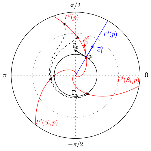
Figure 1: Limit cycle $\Gamma$ (thin black line) and its isochrons (thin red lines) for $\delta>0$, $\kappa>0$ and $\beta>0$ at $p$ and at the image of $p$ by the flow at times $t_{1}=T/3$ and $t_{2}=2T/3$. Trajectories starting from three points on $I^{\beta}(p)$, are represented by a dashed line. One of them belongs to $\Gamma$ and overlaps the thick black line representing it. The states of the trajectories at times $0$, $t_{1}$ and $t_{2}$ are represented by black dots. The isochron at $p$ for vanishing $\beta$ is also represented in blue. Finally, the vectors $\vec{e}_{1}$ associated with the characteristic exponent $-2\delta$ and tangent to the isochrons at $p$ are also plotted for $\beta\neq 0$ and $\beta=0$.

2.3.3 Phase diffusion equation

After introducing the change of variable $(r,\theta)\to(r,\phi)$ according to (2.20) and such that $d\phi/dt=\omega_{f}$ for a deterministic trajectory of the normal form (2.1), one can now apply Itô’s formula (IW, 89, Theorem 5.1) to derive the SDE corresponding to (2.8) in coordinates $(r,\phi)$. Hence, one finds the following phase diffusion equation

$$\,\mathrm{d}r =(\delta r-\kappa r^{3}+\frac{\epsilon^{2}}{2r})\,\mathrm{d}t+\epsilon\,\mathrm{d}W_{r}$$ (2.21)

$$\,\mathrm{d}\phi =\omega_{f}\,\mathrm{d}t+\epsilon\frac{\,\mathrm{d}W_{\theta}}{r}-\tilde{\beta}\epsilon\frac{\,\mathrm{d}W_{r}}{r}.$$

As expected, the $\phi$-component of the drift is now independent of the radius, as in the deterministic case. This is, however, to the expense of the statistical dependence of the noise terms acting on $r$ and $\phi$. The phase $\phi$ thus experiences advection at constant angular velocity $\omega_{f}$ together with nonuniform diffusion. As a consequence, the Kolmogorov equation (2.9) with $u^{\prime}(r,\phi,t)=u(r,\theta,t)$ becomes

$$\partial_{t}u^{\prime}=\left(\delta r-r^{3}+\frac{\epsilon^{2}}{2r}\right)\partial_{r}u^{\prime}+\omega_{f}\partial_{\phi}u^{\prime}+\frac{\epsilon^{2}}{2}\partial^{2}_{rr}u^{\prime}-\frac{\tilde{\beta}\epsilon^{2}}{r}\partial^{2}_{r\phi}u^{\prime}+\frac{\epsilon^{2}(1+\tilde{\beta}^{2})}{2r^{2}}\partial^{2}_{\phi\phi}u^{\prime}.$$ (2.22)

Compared to (2.9), the coefficients in front of the first-order differential operators associated with the drift in (2.22) are now separated in their arguments, here in their $r$- and $\phi$-dependences. This feature is key to the derivation of small-noise expansion of the RP spectrum in Section 4. As a by-product, however, the dependence of the angular frequency on the radius for $\beta\neq 0$ is responsible for an effective increase of the phase diffusion by a factor $1+\tilde{\beta}^{2}$; cf. the coefficient in front of $\partial^{2}_{\theta\theta}$ in (2.9). This effect could have been anticipated from the nonnormality of the polar Jacobian $J_{\Gamma}$ and is explained in greater detail in light of the Hörmander theorem in Section 3 below.

Remark 4

Equations of the type (2.21) and (2.22) for more general systems with an adiabatic phase reduction have recently received much attention for the study of the impact of noise on nonlinear oscillators in physics and engineering; see e.g. DMR (00); DKVJ (09); BCM (13); BCG (14).

3 Analysis of the stochastic Hopf bifurcation

In this section, we apply the stochastic analysis approach as (briefly) surveyed in (CTND, 20, Appendix A), to study the general properties of the Markov semigroup of the SHE (2.6) and its spectrum for any values of the parameters $\delta,\gamma$ and $\beta$, and for $\kappa>0$. The material presented in this section is mostly known by the expert working on the ergodic theory of stochastic systems but contains also useful insights about the role played by the the geometric structures organizing the underlying dynamics and their interactions with the noise. In that respect, Theorem 1 provides interesting relationships between the isochrons of Sec. 2.3 and the violation of the Hörmander condition, positioning thus the material exposed hereafter to be also useful for the expert, while having in mind a wider audience in the geosciences and macroscopic physics.

We start by showing in Sec 3.1 below how the existence of a unique ergodic and smooth invariant measure to SHE (2.6) as well as its mixing properties, relate directly to the configuration of the stochastic forcing with respect to the isochrons. The existence of a spectral gap at the bifurcation and the exponential decay of correlations is then proved in Section 3.2.

3.1 Smoothing and mixing by the noise: a geometric perspective

We have discussed in Section 2 how the tilt of the isochrons, as measured by the twist factor $\tilde{\beta}$, is associated with an increase of the diffusion coefficient in the phase in the Kolmogorov equation (2.22) by a factor $1+\tilde{\beta}^{2}$. This simple result shows the importance of the underlying geometry of the drift and diffusion operators in the study of the ergodic properties of continuous Markov processes. The novel approach which is followed in this section is to place the isochrons in the context of stochastic analysis and to show in Theorem 1 that, for fairly general nonlinear oscillators with diffusion, the smoothing and mixing effects of the noise may critically depend on the interaction of the stochastic forcing fields with the isochrons.

Recall that, according to Doob’s theorem Doo (48), the existence of at most one ergodic invariant measure with a smooth Lebesgue density for a continuous Markov process is a consequence of the regularity of the Markov semigroup $P_{t}$; see e.g. (DZ, 96, Chap. 4). A result, due to Kha (60), shows that the regularity of the Markov semigroup is in turn ensured from the irreducibility and the strong Feller property of the Markov semigroup. The irreducibility and strong Feller properties follow from the controllability of the corresponding control system SV (72) the (hypo-)ellipticity of the operators, respectively.

This well-known approach is used in Proposition 4 to show that the measure $\mu$ with density $\rho_{\infty}$ given by (2.11) is the unique invariant measure of the SHE (2.6). It is recalled in (CTND, 20, Appendix A.2) for the unfamiliar reader that along with (CTND, 20, Theorem 4) relating the smoothness and the strong mixing property of the invariant measure to the strong Feller and irreducibility properties of Markov semigroup. This approach is summarized here by the diagram shown in Fig. 2.

Figure 2: Schematic of the strong Feller-irreducibility approach to prove the existence and uniqueness of a smooth invariant measure for a continuous Markov process.

Yet, the ellipticity of the Kolmogorov operator (2.7) stems from the fact that noise is added to both coordinates of the two-dimensional SHE (2.6). To reveal the role played by the isochrons from a stochastic analysis perspective, we consider next degenerate cases in which noise is not added to both coordinates and study under which conditions the corresponding Markov semigroup is still strongly Feller and irreducible, and thus has a smooth density.

To do so, we rely on the Hörmander theorem for hypoelliptic operators Hör (68). For further reference, we recall the Hörmander’s bracket condition for an SDE on $\mathbb{R}^{N}$ written in its Stratonovich interpretation for $m$ independent 1D Wiener process $W_{i}$,

$$\,\mathrm{d}x=V_{0}(x)dt+\sum_{i=1}^{m}V_{i}(x)\circ\,\mathrm{d}W_{i}.$$ (3.1)

One defines the following collection of vector fields $\mathcal{V}_{k}$ by

$$\mathcal{V}_{0}=\{V_{i}:1\leq i\leq m\},\quad\mathcal{V}_{k+1}=\mathcal{V}_{k}\cup\{[U,V_{j}]:U\in\mathcal{V}_{k}\enskip\&\enskip 0\leq j\leq m\}.$$ (3.2)

The main assumption to be checked for application of the Hörmander theorem is then the following Hörmander bracket condition

$$\cup_{k\geq 1}\mathrm{span~{}}\{V(q):V\in\mathcal{V}_{k}\}=\mathbb{R}^{N}\quad\text{for every}\quad q\in\mathbb{R}^{N},$$ (3.3)

3.1.1 The case of the SHE (2.6) with degenerate noise

Let us consider the following modification of the SHE (2.8) written in Stratonovich form,

$$\,\mathrm{d}X=V_{0}(X)\,\mathrm{d}t+V_{1}(X)\circ\,\mathrm{d}W_{1}.$$ (3.4)

In (3.4), $V_{0}$ denotes the deterministic vector field in (2.8). However, whereas the original SHE (2.8) is driven by two one-dimensional Wiener processes $W_{r}$ and $W_{\theta}$, (3.4) is driven by a single one-dimensional Wiener process $W_{1}$ with an arbitrary smooth vector field $V_{1}$ of $\mathbb{R}^{2}$.

Using the coordinate-free formalism (see Remark 5 below), the Kolmogorov operator $\mathcal{K}$ associated with (3.4) can be written as

$$\mathcal{K}=V_{0}+(V_{1})^{2}.$$

Here, as opposed to the original SHE (2.6) we have chosen $V_{1}$ to be nonconstant and to be multiplied by a one-dimensional Wiener process, only. Thus, at each point $q$ in $\mathbb{R}^{2}$, the vector $V_{1}(q)$ alone cannot span $\mathbb{R}^{2}$ and the Kolmogorov operator $\mathcal{K}$ is no longer elliptic. It may turn out, however, that the operator is hypoelliptic, ensuring, roughly speaking, to have the noise to propagate out in the whole space; see next subsection. Our aim is then to check under which condition on $V_{1}$ the Kolmogorov operator $\mathcal{K}$ is hypoelliptic. For that purpose we need to verify under which conditions the Hörmander condition (3.3) holds.

We thus calculate the Lie bracket of $V_{1}$ with $V_{0}$. The vector fields $V_{0}$ and $V_{1}$ are given in polar coordinates by

$$V_{0}(r,\theta) =F(r,\theta)=(\delta r-\kappa r^{3})~{}\partial_{r}+(\gamma-\beta r^{2})~{}\partial_{\theta}$$

$$V_{1}(r,\theta) =V_{1}^{r}(r,\theta)~{}\partial_{r}+V_{1}^{\theta}(r,\theta)~{}\partial_{\theta},$$

where $V_{1}^{r}$ and $V_{1}^{\theta}$ are the (smooth) components of $V_{1}$. Let us first consider the simple yet instructive case when

$$V_{1}^{r}=\epsilon_{r},\quad\mathrm{and}\quad V_{1}^{\theta}=0,$$

for some constant $\epsilon_{r}>0$. Then the Lie bracket $[V_{0},V_{1}]$ yields

$$[V_{0},V_{1}]=-\epsilon_{r}(\delta-3\kappa r^{2})~{}\partial_{r}-2\epsilon_{r}\beta r~{}\partial_{\theta}.$$ (3.5)

Observe that $\mathrm{span~{}}\mathcal{V}_{1}=\mathrm{span~{}}\{V_{1},[V_{0},V_{1}]\}=\mathbb{R}^{2}$ if and only if $\beta$, or equivalently the twist factor $\tilde{\beta}$, is nonzero. This is also true when further iterating the Lie brackets.

Thus, even in the case of a purely radial stochastic forcing, the twist of the isochron controlled by $\tilde{\beta}$ allows for the noise to be injected in the azimuthal direction and for the Markov semigroup to be strongly Feller. This also explains the increase by a factor $1+\tilde{\beta}^{2}$ of the diffusion coefficient in the Kolmogorov equation (2.22) written in the phase-coordinate, compared to that of (2.9) written in polar coordinates. It will have also important consequences on the RP eigenfunctions in Section 4. On the other hand, if $\beta=0$ and $V_{1}$ is radial, the noise is not felt in the azimuthal direction and no phase diffusion may occur.

This result is illustrated in Fig. 3 for the SHE (2.6) with $\delta=\kappa=1$ and $\beta=0$ (upper panels) and $\beta=0.8$ (lower panels). On the left panels, the Lie bracket $[V_{0},V_{1}]$, for $V_{1}=\epsilon_{r}~{}\partial_{r}$ (blue vector), is applied to a point $p$. There, $S_{t}$ and $S_{t}^{V_{1}}$ are the flows generated by $V_{0}$ and $V_{1}$, respectively, and $\delta t$ is a small time. The Lie bracket (red vector in Fig. 3) is given by the tangent vector to the curve obtained by successively applying $S_{\delta t}$ and $S_{\delta t}^{V_{1}}$ forward and then backward in the limit when $\delta t\to 0$. On the right panels, samples of simulated time series of the asymptotic phase $\phi$ given by (2.20) are represented. One observes that when $\beta=0$ (upper panels of Fig. 3), the integral curves of the forcing field $V_{1}$ (dashed blue lines in Fig. 3) coincide with the isochrons (red lines in Fig. 3) and the resulting Lie bracket is collinear to $V_{1}$, in agreement with (3.5). As a result, no phase diffusion is observed on the corresponding upper right panel of Fig. 3.

On the other hand, when $\beta$ is nonzero (lower panels), the forcing field $V_{1}$ is not tangent to the isochrons anymore and the resulting Lie bracket is not collinear to $V_{1}$. This allows for the noise to be injected in the azimuthal direction, as can be seen from the phase diffusion occurring in the lower right panel of Fig. 3. This figure reveals that the dependence of the Lie bracket (3.5) on the twist factor $\tilde{\beta}$ is directly related to the orientation of the forcing field $V_{1}$ with respect to the isochrons. This observation will now be made rigorous for the more general case of a dynamical system with a hyperbolic limit cycle.

Remark 5

In the coordinate-free framework of differential geometry, a vector field $V$ defined on the plane $\mathbb{R}^{2}$ and decomposed in Cartesian coordinates as $V(x,y)=V^{1}(x,y)\vec{e}_{1}+V^{2}(x,y)\vec{e}_{2}$, is identified (by isomorphism) with the first-order differential operator

$$V=V^{1}(x,y)~{}\partial_{x}+V^{2}(x,y)~{}\partial_{y}.$$

See e.g. Fec (06) for an introduction to differential geometry.

3.1.2 Hörmander bracket condition for a general hyperbolic limit cycle

For more generality, let us consider a dynamical system with flow $S_{t},t\geq 0$, generated by the smooth vector field $V_{0}$ on the $N$-dimensional Euclidean space $\mathbb{R}^{N}$. Assume that the flow has a hyperbolic limit cycle $\Gamma$ with basin of attraction $U_{\Gamma}\subseteq\mathbb{R}^{N}$, so that the isochrons $W_{ss}(p)$ at any point $p$ on $\Gamma$ can be defined as the stable foliation of $\Gamma$; see Section 2. Consider then the SDE (3.1) in which the deterministic field $V_{0}$ is perturbed by $m$ smooth vector fields $\{V_{i},{\color[rgb]{0,0,0}1\leq i\leq m}\}$ each multiplied by independent one-dimensional Wiener processes. We would like to know when the interaction of this stochastic forcing with the isochrons allows for the parabolic Hörmander condition (3.3) in $U_{\Gamma}$ to be fulfilled. The following Theorem 1 is proved in Appendix B.1, as a direct consequence of the definition of the Lie derivative in terms of pullback of a vector field by a diffeomorphism.

Theorem 1

If, for some point $q$ in $U_{\Gamma}$, the vector fields $\{V_{i},{\color[rgb]{0,0,0}1\leq i\leq m}\}$ of the stochastic forcing in (3.4) are all tangent to the isochron $W_{ss}(p)$ passing through $q$, then the vector space

$$\cup_{k\geq 1}\mathrm{span~{}}\{V(q):V\in\mathcal{V}_{k}\},$$

generated by the vector fields $V_{0}$ and $\{V_{i},{\color[rgb]{0,0,0}1\leq i\leq m}\}$ according to (3.2) is also tangent at $q$ to the isochron $W_{ss}(p)$.

Keeping the same notations, the contraposition of Theorem 1 yields the following corollary.

Corollary 1

For the parabolic Hörmander condition (3.3) to be fulfilled, it is necessary that, for each point $q$ in $U_{\Gamma}$, at least one of the vector fields in $\{V_{i},{\color[rgb]{0,0,0}1\leq i\leq m}\}$ is transverse to the isochron passing through this point.

The dependence of the Lie bracket $[V_{0},V_{1}]$ on the twist factor $\tilde{\beta}$ in Fig. 3 is now understood thanks to Theorem 1 in terms of orientation of the forcing vector field $V_{1}$ with respect to the isochrons. There, $V_{1}$ acts on the radial direction only. For $\beta=0$ (upper panels), the isochrons are rectilinear and coincide with the integral curves of $V_{1}$. In agreement with Theorem 1, the Lie bracket $[V_{0},V_{1}]$ is also tangent to the isochrons. Thus,

$$\cup_{k\geq 1}\mathrm{span~{}}\{V(q):V\in\mathcal{V}_{k}\}=TW_{ss}(p)\neq\mathbb{R}^{2},$$

and the Kolmogorov operator $\mathcal{K}$ is not hypoelliptic, which explains the absence of phase diffusion on the upper right panel. For $\beta\neq 0$ (lower panels), however, the stochastic field $V_{1}$ is not tangent to the isochrons anymore. As a consequence and in agreement with (3.5), the Lie bracket $[V_{0},V_{1}]$ is able to span the azimuthal direction, so that the Hörmander condition (3.3) is fulfilled. It follows that the Kolmogorov operator $\mathcal{K}$ is hypoelliptic, by Hörmander’s theorem, which is manifested by the occurrence of phase diffusion in the lower right panel of Fig. 3.

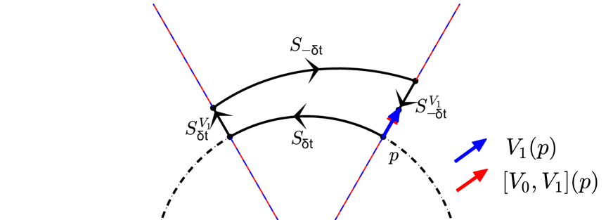
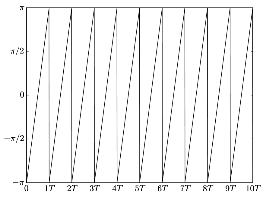
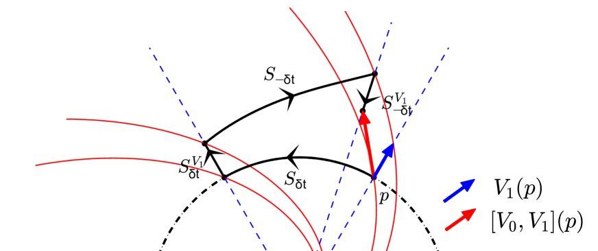
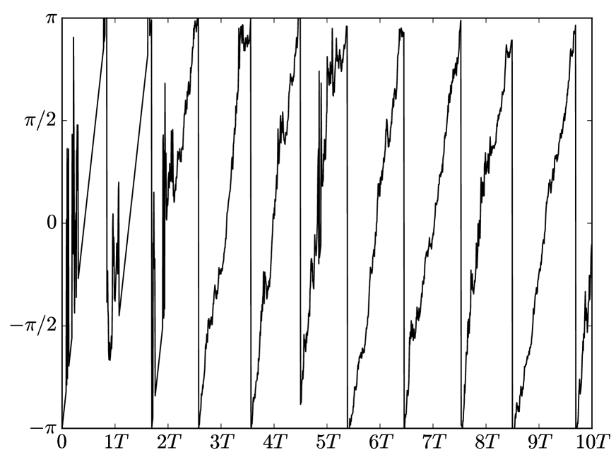
Figure 3: Left: Illustration of the action of the Lie bracket $[V_{0},V_{1}]$ (red arrow) at a point $p$ between the vector field $V_{0}$ generating the autonomous flow $S_{t},t\geq 0$ with the forcing field $V_{1}$ (blue arrow at $p$) generating the flow $S_{t}^{V_{1}},t\geq 0$ in the radial direction for $\beta=0$ (upper panels) and $\beta\neq 0$ (lower panels). The thick black curve represents the composition of the two flows for a short time ${\delta t}$ and then back. The isochrons passing through the different images of the initial point $p$ by the flow are represented by a thin red line, while the integral curves of the forcing field $V_{1}$ are represented by dashed blue lines. Right: Sample time series of the phase $\phi$ corresponding to the left panels when the forcing field $V_{1}$ acts on a Wiener process as in the SDE (3.4).

3.2 Spectral gap property of the SHE (2.6)

We now turn to the spectral properties of the Markov semigroup of the SHE (2.6) and to the nature of the decay of correlations depending on the control parameter $\delta$ and $\kappa$ and for $\epsilon>0$. In this case, recall that the diffusion operator,

$$D=\epsilon^{2}(\partial^{2}_{xx}+\partial^{2}_{yy}),$$

in Cartesian coordinates in the right-hand side of (2.7), is uniformly elliptic, in the sense that there exists $\alpha>0$ such that,

$$\left<\xi,D\xi\right>\geq\alpha\|\xi\|^{2},\quad\forall\xi\in\mathbb{R}^{2}.$$

In addition exponential decay of correlation is expected below the bifurcation point, for $\delta<0$, since, for the deterministic case, the RP spectrum in spaces of distributions has a spectral gap GT (01). However, this is not the case above the bifurcation for which some resonances are on the imaginary axis and prevent mixing, nor is it the case exactly at the bifurcation point where the RP spectrum is continuous and responsible for an algebraic decay of correlations. The latter is not possible here, since we know that the spectrum of the SHE (2.6) is discrete (see Sect. 2.2). We also know from the previous Section 3.1 that purely imaginary are not to be expected since the invariant measure is strongly mixing. Yet an accumulation point at 0 in the complex plain could still prevent the existence of a spectral gap.

The following proposition states that, for all values of the control parameter $\delta$, a spectral gap in fact exists in $L^{2}_{\mu}(\mathbb{R}^{2})$, where $\mu$ is the invariant measure associated with the density $\rho_{\infty}$ (Eq. (2.11)). The proof is given in Appendix B.2 and relies on the theory of Lyapunov functions and ultimate bounds reviewed in (CTND, 20, Appendix A.5).

Proposition 3

For any $\delta$ in $\mathbb{R}$, $\beta$ in $\mathbb{R}$, $\kappa>0$ and $\epsilon>0$, the SHE (2.6) has a spectral gap and correlations decay exponentially in $L^{2}_{\mu}(\mathbb{R}^{2})$.

This result is thus just a consequence of stochastic analysis techniques as reviewed in CTND (20), without explicit calculations of the RP spectrum. In Section 4 below, we provide however a more precise description of the latter by using small-noise expansion techniques; see Propositions 4 and 5.

Remark 6

Note that for $\delta<0$, the rate $2\delta$ of the exponential bound in (B.4) is given by the real part of the second eigenvalue of the Kolmogorov operator of the linearized system at the origin, i.e. the leading eigenvalue associated with an eigenfunction on which the projection of $\varphi(r,\theta)=r^{2}$ is nonzero; see Section 4.1.

Remark 7

Interestingly, for $\delta=0$ and $\epsilon=0$, the ultimate bound is, however, not verified. This is not surprising, since we know from GT (01) that the decay of correlation is in this case only algebraic. On the other hand, for $\delta\neq 0$ but $\epsilon=0$, the ultimate bound still holds but one cannot apply Theorem 6 from CTND (20) anymore, since the system is no longer stochastic. However, the existence of a spectral gap and the exponential decay of correlations in this deterministic case may be inferred from GT (01).

4 Small-noise approximation of the RP resonances, $\delta\neq 0$

In this section, we look for expansions of the RP eigenvalues and eigenfunctions for relatively low values of the noise level $\epsilon>0$ and away from the bifurcation as singular perturbations of the deterministic case.

General small-noise expansion formulas for the RP resonances have been derived by Gas (02) using a WKB approximation and his results have been discussed for a form of the SHE (2.6) considered here by Bag (14). However, to learn more about the geometrical properties of the stochastic system and to be able to calculate power spectra between any pair of observables according to the spectral decomposition (1.7), we derive analytic approximations of the eigenfunctions of the Kolmogorov operator $\mathcal{K}$ as well as of those of its adjoint, $\mathcal{K}^{\ast}$.

To do so, we rely on a rescaling of the coordinates depending both on the noise level $\epsilon$ and on the parameter $\delta$ controlling the stability of the solutions to adimensionalize the SHE (2.6). A natural time scale is given by $\delta^{-1}$, while a spatial scale $L_{\epsilon}(\delta)$ capturing the effect of the noise with respect to the stability of the deterministic solutions is given by $\epsilon/\sqrt{-\delta}$ if $\delta<0$ or by $\epsilon/\sqrt{\delta}$ if $\delta>0$. Applying Itô’s formula, the change of variable $r\to r^{\prime}=r/L_{\epsilon}(\delta)$, $\theta\to\theta^{\prime}=\theta$ or $\phi\to\phi^{\prime}=\phi$, and $t\to t^{\prime}=\delta t$ yields for the SHE (2.6),

$$\,\mathrm{d}r^{\prime} =r^{\prime}\left(\frac{\delta}{|\delta|}-\frac{r^{\prime 2}}{r_{\epsilon}^{2}}+\frac{1}{2r^{\prime 2}}\right)\,\mathrm{d}t^{\prime}+\,\mathrm{d}W_{r}$$ (4.1)

$$\,\mathrm{d}\theta^{\prime} =\left(\tilde{\gamma}-\tilde{\beta}\frac{r^{\prime 2}}{r_{\epsilon}^{2}}\right)\,\mathrm{d}t^{\prime}+\frac{\,\mathrm{d}W_{\theta}^{\prime}}{r^{\prime}}$$

$$\mathrm{or~{}}\,\mathrm{d}\phi^{\prime} =\left(\tilde{\gamma}-\tilde{\beta}\right)\,\mathrm{d}t^{\prime}-\tilde{\beta}\frac{\,\mathrm{d}W_{r}}{r^{\prime}}+\frac{\,\mathrm{d}W_{\theta}}{r^{\prime}},$$

where $\delta/|\delta|=-1$ if $\delta<0$, $1$ if $\delta>0$. In addition to the twist factor $\tilde{\beta}=\beta/\kappa$, we have introduced the adimensional parameters $\tilde{\gamma}(\gamma,\delta)=\gamma/\delta$ and $r_{\epsilon}(\delta,\kappa)=\delta/(\sqrt{\kappa}\epsilon)$, simply noted $\tilde{\gamma}$ and $r_{\epsilon}$, respectively, in the remaining. Defining $R$ by $\sqrt{-\delta/\kappa}$ for $\delta<0$, the adimensional parameter is such that $r_{\epsilon}=R/L_{\epsilon}(\delta)$. Thus the effect of the noise on the adimensional dynamics (4.1) is bound to that of the parameters $\delta$ and $\kappa$ in a single coefficient $r_{\epsilon}$. For a fixed $R$, this effect increases with the noise-level $\epsilon$ and decreases with the square root of $\delta$. Since all coefficients in (4.1) involving the noise level $\epsilon$ enter as $\sigma_{\epsilon}=1/r_{\epsilon}$, we are led to expand the eigenvalues and eigenfunctions of the Kolmogorov operator as,

$$\lambda =\lambda^{(0)}+\sigma_{\epsilon}\lambda^{(1)}+\sigma_{\epsilon}^{2}\lambda^{(2)}+\dots$$

$$\psi^{\prime} =\psi^{(0)}+\sigma_{\epsilon}\psi^{(1)}+\sigma_{\epsilon}^{2}\psi^{(2)}+\dots.$$

Since, the deterministic solutions and the change of variables differ for $\delta<0$ and $\delta>0$, each case is treated separately in the next subsections 4.1 and 4.2, respectively. From the definition of the small parameter $\sigma_{\epsilon}$, whether for $\delta<0$ or for $\delta>0$, the small-noise expansions will be more precise when the noise level $\epsilon$ is small with respect to $\delta$, for a fixed $\kappa$.

4.1 Below the bifurcation ($\delta<0$)

All deterministic solutions converge to the steady state $x_{*}$ at the origin. An example of stochastic trajectory is represented in blue in Fig. 4-(a) for $\delta=-1$, $\kappa=1,\gamma=4,\beta=0.5$ and $\epsilon=0.4$ on top of the corresponding stationary density given by (2.11). As expected, the process meanders near, $x_{*}$, although the maximum in density is slightly away from $x_{*}$, due to the additional drift term $\epsilon/(2r)$ in (2.8). The following proposition yields the small-noise expansion of the leading part of the spectrum of the SHE (2.6) for $\delta<0$. The proof is given in Appendix C.1 and relies on known results for the complex Ornstein-Uhlenbeck process MPP (02); CL (14).

Proposition 4

For $\delta<0$ and $\epsilon\sqrt{\kappa}/\delta<<1$ the approximation of the leading eigenvalues and eigenfunctions associated with the SHE (2.6) are given by:

• Eigenvalues associated with the stable steady state:

  $$\lambda_{ln}=(l+n)\delta+i(n-l)\gamma+\mathcal{O}_{\tilde{\beta}}\left(\left(\frac{\epsilon/\sqrt{\delta}}{\sqrt{\delta/\kappa}}\right)^{2}\right),\quad l,n\in\mathbb{N}.$$ (4.2)

• Eigenfunctions associated with the stable steady state:

  $$\psi_{ln}(r,\theta)\approx\begin{cases}e^{i(n-l)\theta}\enskip\sqrt{\frac{l!}{n!}}\left(\sqrt{-\frac{\delta}{\epsilon^{2}}}r\right)^{n-l}L_{l}^{n-l}\left(-\frac{\delta r^{2}}{\epsilon^{2}}\right),\quad&n\geq l\\ e^{i(l-n)\theta}\enskip\sqrt{\frac{n!}{l!}}\left(\sqrt{-\frac{\delta}{\epsilon^{2}}}r\right)^{l-n}L_{n}^{l-n}\left(-\frac{\delta r^{2}}{\epsilon^{2}}\right),\quad&n<l,\end{cases}$$ (4.3)

  where $L^{\alpha}_{l}(r)=\frac{r^{-\alpha}}{l!}e^{r}\frac{d^{l}}{dr^{l}}(e^{-r}r^{l+\alpha})$ denotes the Laguerre polynomial of degree $l$ (LS, 72, p. 76) in the radius $r$.

• Adjoint eigenfunctions associated with the stable steady state:

  $$\psi^{*}_{ln}\approx\psi_{ln}\enskip\rho_{x_{*}}.$$ (4.4)

• Decorrelation time:

  $$\tau=-\frac{1}{\delta}+\mathcal{O}_{\tilde{\beta}}\left(\left(\frac{\epsilon/\sqrt{\delta}}{\sqrt{\delta/\kappa}}\right)^{2}\right).$$ (4.5)

In (4.2) and (4.5), $\mathcal{O}_{\tilde{\beta}}(\epsilon\sqrt{\kappa}/\delta)$ is the usual asymptotic notation for the small parameter $\epsilon\sqrt{\kappa}/\delta$ but with an indication that the remaining terms in the expansions actually depend on the twist factor $\tilde{\beta}$.

The RP resonances (4.2) are represented in Fig. 4-(c) for fixed values of the parameters. A typical triangular structure is observed, as a result of the aforementioned integer linear combination of complex conjugate eigenvalues $\lambda^{\pm}=\delta\pm i\gamma$ of the tangent map $J_{x_{*}}$. In the direction of the real axis, these eigenvalues are separated by a gap of $\delta$ given by the real part of the eigenvalues of the tangent map. Thus, as the control parameter $\delta$ is increased to its critical value, the decorrelation time $\tau\approx-1/\delta$ in (4.5) increases, indicative of the weaker stability of the steady state of the deterministic system. Moreover, the eigenvalue $\lambda_{ln},n>l$ is associated with an eigenfunction that is approximated by the product of a polynomial of degree $n+l$ and the $(n-l)$th harmonic function $\exp{i(n-l)\theta}$. Thus, eigenfunctions associated with eigenvalues further away from the real axis (resp. imaginary axis) exhibit a higher degree of nonlinearity in the radial (resp. azimuthal) direction, as measured by their number of sign changes. As an example, the eigenfunction $\psi_{01}$ associated with the eigenvalue $\lambda_{01}\approx\delta+i\gamma$ closest to the imaginary axis is represented in Fig. 4-(e). Its phase $\arg\psi_{01}=\theta$ is represented by filled contours, while its amplitude $\psi_{01}e^{-i\arg\psi_{01}}=r$ is represented by dashed contour lines. The amplitude and phase of the leading secondary eigenfunction is thus the components of the stochastic process in polar coordinates. This is not surprising, since the eigenfunctions are approximated by those of the (linear) Ornstein-Uhlenbeck process with drift given by the tangent map $J_{x_{*}}$, as explained above.

Remark 8

In the expansion (4.2), we do not control for changes in the weights in front of the $\mathcal{O}(\epsilon^{2})$ for different eigenvalues. Thus, high-order terms may have a larger impact for some eigenvalues than for other, a phenomenon that we describe in the numerical results of Section 5.2.1.

4.2 Above the bifurcation ($\delta>0$)

After the deterministic Hopf bifurcation, two limit sets coexist, the unstable steady state $x_{*}$ at the origin and the stable limit cycle $\Gamma$ of radius $R$. An example of stochastic trajectory is represented in blue in Fig. 4-(b) for $\delta=1.5$, $\kappa=1,\gamma=4,\beta=0.5$ and $\epsilon=0.4$ on top of the corresponding stationary density given by (2.11), while the orbit $\Gamma$ is represented by the dashed line. Here small-noise expansions are also illuminating to obtain approximation formulas when applied separately about the unstable steady state and the limit cycle.

4.2.1 Small-noise expansions about the unstable steady state $x_{*}$

Repeating similar arguments than in the case $\delta<0$, the RP resonances associated with the unstable steady state are here given for $\delta>0$, by

$$\lambda_{ln}=-(l+n+2)\delta-i(l-n)\gamma+\mathcal{O}_{\tilde{\beta}}\left(\left(\epsilon\sqrt{\kappa}/\delta\right)^{2}\right),\quad l,n\in\mathbb{N}.$$ (4.6)

These eigenvalues are represented for fixed values of the parameters as blue triangles in Fig. 4-(d). A triangular array of eigenvalues is found, as for $\delta<0$ in panel (c) of the same figure. However, the real part of these eigenvalues satisfies $\Re(\lambda_{ln})\leq-2\delta.$ The latter bound actually characterizes the rate of expansion of volumes near the unstable steady state $x_{*}$ (and away from the limit cycle $\Gamma$). The latter decreases with increasing $\delta$, i.e. as the instability of $x_{*}$ increases.

4.2.2 Small-noise expansions about the limit cycle $\Gamma$

On the other hand, another family of eigenvalues associated with the limit cycle can be identified. In order to study small-noise perturbations of the system away from the limit cycle, we work in Appendix C.2 from the adimensional version of the Kolmogorov equation (2.22) associated with the radial $r$ and asymptotic phase $\phi$, variables. Compared to the original Kolmogorov equation (2.9) written in polar coordinates, the Kolmogorov equation (2.22) — formulated in Sect. 2.3.3 with the help of isochrons — helps us separate the drift term into two contributions, one in the $r$-coordinate alone, and the other in the $\phi$-coordinate. In the unperturbed case, this separation of variables shows that the isochrons can be identified with isolines of phase of the eigenfunctions associated with purely imaginary eigenvalues. As a result, Fourier averages related to these eigenfunctions have been proposed to estimate the isochrons MM (12); MMM (13). The following proposition, proved in Appendix C.2, shows for the SHE (2.8) that, when the noise is asymptotically small, the isochrons still coincide with the isoline of phase of the eigenfunctions.

Proposition 5

For $\delta>0$ and $\epsilon\sqrt{\kappa}/\delta<<1$ the approximation of the leading eigenvalues and eigenfunctions associated with the limit cycle $\Gamma$ of the SHE (2.6) are given by:

• Eigenvalues associated with the stable limit cycle:

  $$\lambda_{ln}=\begin{cases}-\frac{n^{2}\epsilon^{2}(1+\tilde{\beta}^{2})}{2R^{2}}+in\omega_{f}+\mathcal{O}\left(\left(\frac{\epsilon/\sqrt{\delta}}{\sqrt{\delta/\kappa}}\right){}^{3}\right),\quad&l=0,\quad n\in\mathbb{Z}\\ -2l\delta+in\omega_{f}+\mathcal{O}{\left(\frac{\epsilon/\sqrt{\delta}}{\sqrt{\delta/\kappa}}\right)},\quad&l\neq 0.\end{cases}$$ (4.7)

• Eigenfunctions associated with the stable limit cycle:

  $$\psi_{ln}\approx\left(2^{k}k!\right)^{-\frac{1}{2}}\enskip e^{in\left(\theta-\tilde{\beta}\log{\frac{r}{R}}\right)}\enskip H_{l}\left(\frac{\sqrt{2\delta}}{\epsilon}\left(r-R\right)\right),\enskip\quad l=0.$$ (4.8)

• Adjoint Eigenfunctions of the stable limit cycle:

  $$\psi^{*}_{ln}\approx\left(2^{k}k!\right)^{-\frac{1}{2}}\enskip e^{in\left(\theta+\tilde{\beta}\log{\frac{r}{R}}\right)}\enskip H_{l}\left(\frac{\sqrt{2\delta}}{\epsilon}\left(r-R\right)\right)\enskip\rho_{x_{*}}(r),\enskip\quad l=0.$$ (4.9)

• Decorrelation time:

  $$\tau=\frac{2R^{2}}{\epsilon^{2}(1+\tilde{\beta}^{2})}+\mathcal{O}\left(1\right).$$ (4.10)

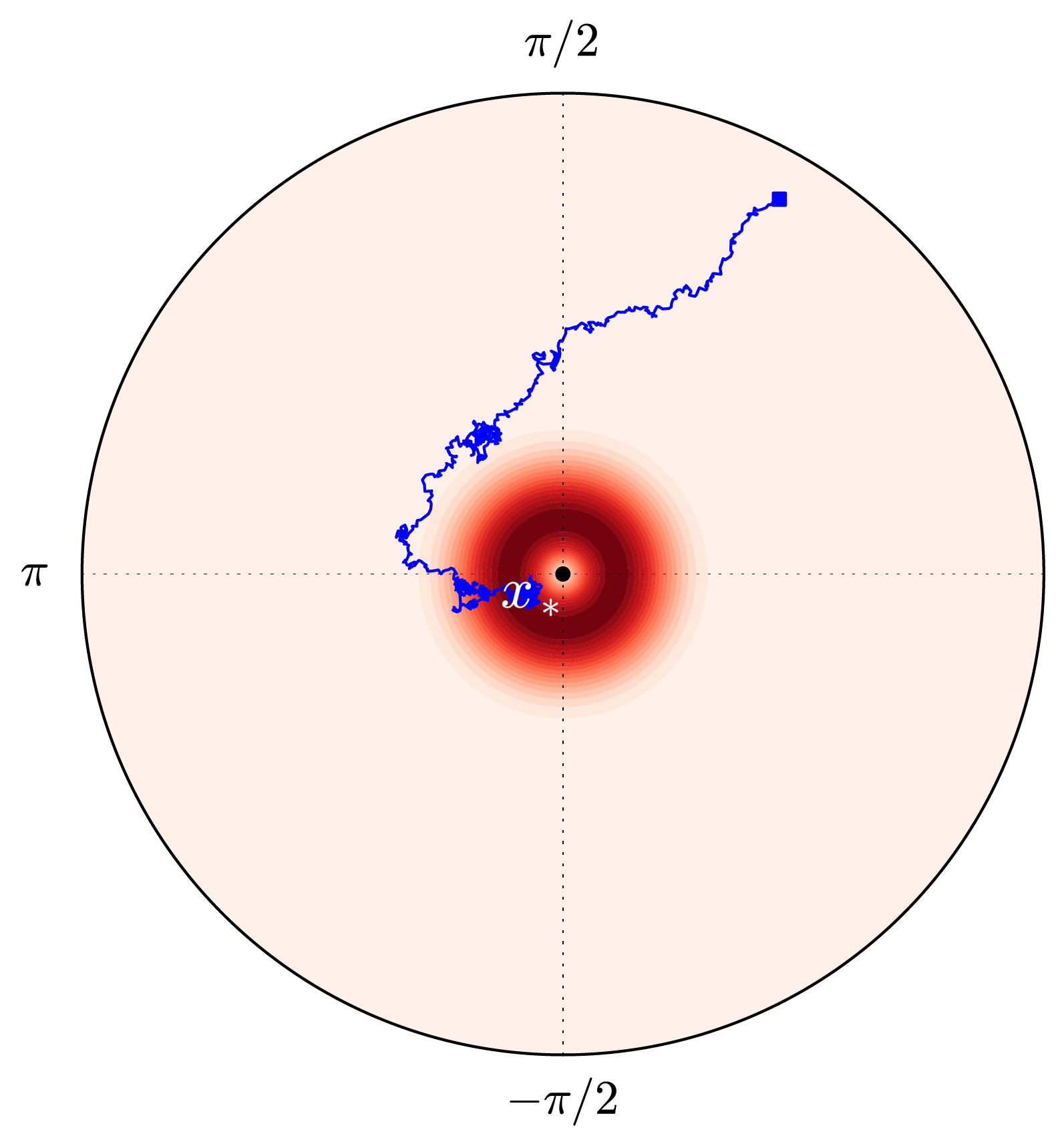
(a)

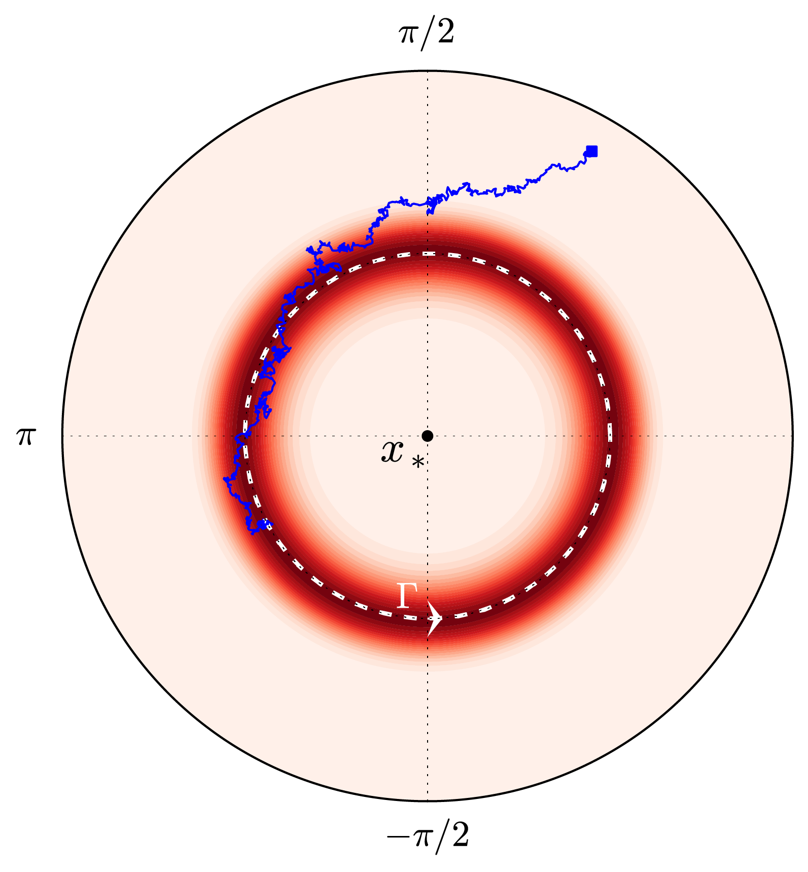
(b)

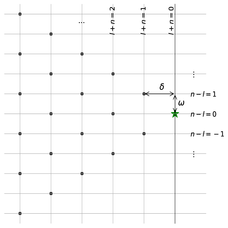
(c)

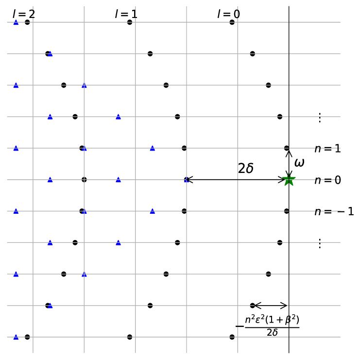
(d)

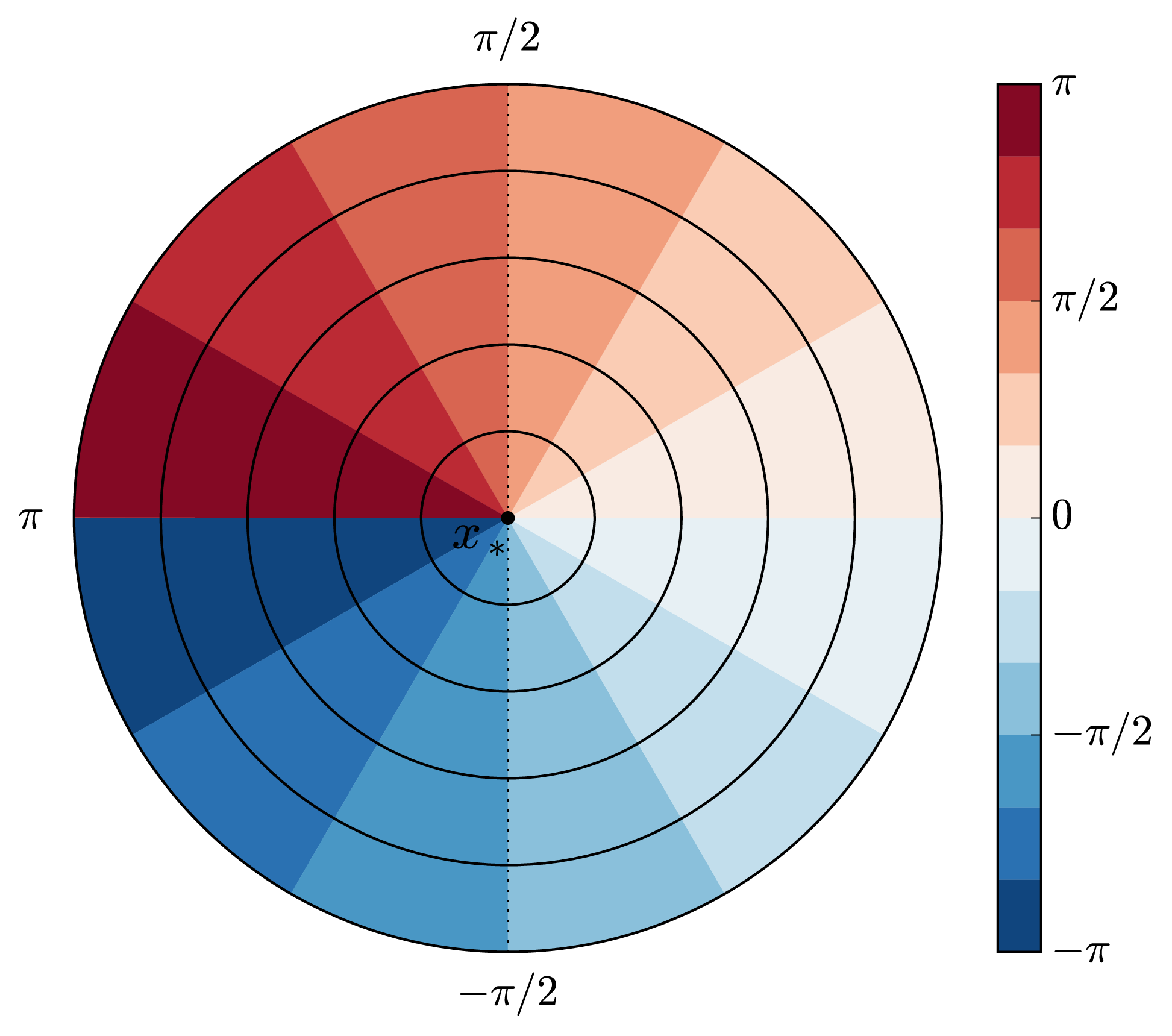
(e)

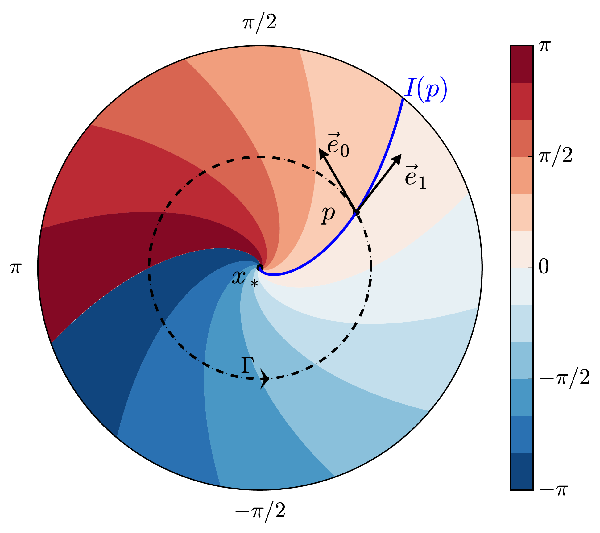
(f)

Figure 4: Schematic of the approximated RP spectrum of the SHE (2.6), for $\kappa=1,\gamma=4,\beta=0.5$ and $\epsilon=0.4$, and with $\delta=-1<0$ (left) or $\delta=1.5$ (right). The top panels (a-b) represent the stationary density (2.11) as red filled contours, together with an example of trajectory in blue and the steady state $x_{*}$ at the origin. The RP resonances in the complex plane are represented in the central panels (c-d), with their real parts as abscissa and their imaginary parts as ordinates. The bottom panels (e-f) represent the second eigenfunction $\psi_{01}$, with its phase as filled contours and its amplitude as thin line contours (for $\delta<0$). For $\delta>0$, the deterministic limit cycle $\Gamma$ is also represented as a thick dashed line, together with the isochron $I_{x_{0}}$ of some point $x_{0}$ on $\Gamma$ as a thick blue line and the eigenvectors $\vec{e}_{0}$ and $\vec{e}_{1}$ of the tangent map at this point.

To help interpret these formulas, the RP resonances for fixed values of the parameters are represented in Fig. 4-(d) together with the eigenfunction $\psi_{01}=\exp{i(\theta-\tilde{\beta}\log{r/R})}$ associated with the second eigenvalue $\lambda_{01}=-\epsilon^{2}(1+\tilde{\beta}^{2})/(2R^{2})+in\omega_{f}$ in Fig. 4-(f). One can first observe in panel (d) a typical array of parabolas of eigenvalues. The latter are separated by a spectral gap of $-2\delta$ (see Remark 6) given by the characteristic exponent associated with the Floquet vector transverse to the flow and accounting for the stability of the limit cycle $\Gamma$; see also A. One the other hand, the imaginary part $in\omega_{f}$, for each harmonic, is associated with the neutral dynamics of advection along the limit cycle. These two contributions jointly coincide with the eigenvalues for the deterministic case found in spaces of distributions by GT (01).

However, the diffusion along the limit cycle, is responsible for an additional real contribution $-n^{2}\epsilon^{2}(1+\tilde{\beta}^{2})/(2R^{2})$, which is not found in the deterministic case and which is responsible for the parabolic shape of the array of eigenvalues. As a result, $\lambda_{00}=0$ (represented as a green star in Fig. 4-(d)) is the only eigenvalue on the imaginary axis. The presence of noise therefore enforces the system to be mixing, in agreement with the spectral gap result of Section 3.2. This “loss of memory” is captured by the finiteness of the decorrelation time $\tau\approx 2R^{2}/(\epsilon^{2}(1+\tilde{\beta}^{2}))$, which decreases as the noise level $\epsilon$ and the curvature $1/R$ of $\Gamma$ strengthen.

In addition, the phase diffusion becomes stronger with increasing magnitude of the twist factor $\tilde{\beta}$ as well. As discussed in Section 3.1, a nonvanishing twist factor $\tilde{\beta}$ allows for a fraction of the noise in the radial direction to be transmitted to the azimuthal direction by the deterministic vector field $F$. As depicted in panel (f) of Fig. 4, the eigenvector $\vec{e}_{2}$ of the tangent map to $F$ is tangent to $\Gamma$, while $\vec{e}_{1}$ is tangent to the isochron. Thus, when $\beta\neq 0$, the vector $\vec{e}_{1}$ projects both on the radial and on the azimuthal parts of the stochastic forcing. Moreover, since $\arg\psi_{01}=\phi=\theta-\tilde{\beta}\log(r/R)$, the phase of the second eigenfunction follows the isochrons, so that the radial dependence of the phase diffusion results in the characteristic twisting of the eigenfunctions when $\beta\neq 0$. As a result, the eigenfunctions are not orthogonal when $\beta$ is nonzero and the Kolmogorov operator $\mathcal{K}$ inherits from the nonnormality of the Jacobian $J_{\Gamma}$. Finally, (C.6) and (4.8) show that the eigenfunctions associated with eigenvalues further from the real axis (imaginary axis) have a higher degree of nonlinearity in the radius (resp. the phase).

To conclude, let us emphasize the difference in structure between the RP spectrum associated with the stable steady state for $\delta<0$ and the one associated with the limit cycle for $\delta>0$. While the eigenvalues have nonvanishing imaginary parts in both cases (4.2) and (4.7), which must result in peaks in the power spectrum, the triangular structure for the steady state and the parabolic structure for the limit cycle, as shown in Fig. 4-(c) and Fig. 4-(d), allow one to discriminate between stochastically forced linear oscillations and nonlinear oscillations with phase diffusion. This is also true regarding the eigenfunctions, given by the formulas (4.3) and (4.8), which in the case of the steady state (and to zeroth order) are the product of different polynomials by harmonics with a different sensitivity to the twist factor $\tilde{\beta}=\beta/\kappa$. These effects will be illustrated in the applications of the third part of this contribution TCND (19), with a discussion of their use to characterize the nature of the dynamics of complex oscillatory systems. The investigation of the RP spectrum at the bifurcation does not follow the reasoning above. Instead, we numerically investigate mixing at the bifurcation in the following Section 5.

5 Mixing at the bifurcation point: Numerical results

Close to the bifurcation point, the small noise-expansions of the previous Section 4 are no longer valid since the linear term in $\delta$ vanishes and the rescaling of time in terms of this parameter is no longer possible. We thus perform a complementary numerical analysis of the Kolmogorov equation to study the RP spectrum at the critical point and test the range of validity of the analytical formulas of the previous Section 4.

5.1 A different scaling

Let us first note that, even though the limit cycle does not exist, the asymptotic phase $\phi$ for any point different from the origin can still be defined up to a constant as $\phi=\theta-\tilde{\beta}\log{r}$ and such that the derivative (2.19) exists and the Kolmogorov equation (2.22) in $(r,\phi)$ coordinates holds. Second, contrary to the deterministic case, a new temporal scale can be defined as $(\epsilon\sqrt{\kappa})^{-1}$ when $\epsilon>0$. A corresponding spatial scale may then be defined as $\epsilon^{1/2}/\kappa^{1/4}$. This time scale thus depends on the coefficient $\kappa$ of the cubic term of the radial vector field in (2.8) rather than on the coefficient $\delta$ of the linear term used in Section 4 for $\delta\neq 0$, and the spatial scale is now proportional to $\sqrt{\epsilon}$ rather than to $\epsilon$. We thus use the following change of variable to adimensionalize the SHE (2.6),

$$r^{\prime}=r\kappa^{1/4}/\epsilon^{1/2},\quad\phi^{\prime}=\phi+\omega_{f}t\quad s=\epsilon\sqrt{\kappa}t.$$

Indeed, the Kolmogorov equation (2.22) with $u^{\prime}(r^{\prime},\phi^{\prime})=u(r,\phi)$ then becomes

$$\partial_{s}u^{\prime}=(-r^{\prime 3}+\frac{1}{2r^{\prime}})\partial_{r^{\prime}}u^{\prime}+\frac{1}{2}\partial^{2}_{r^{\prime}r^{\prime}}u^{\prime}-\frac{\tilde{\beta}}{r^{\prime}}\partial^{2}_{r^{\prime}\phi^{\prime}}u^{\prime}+\frac{1+\tilde{\beta}^{2}}{2r^{\prime 2}}\partial^{2}_{\phi^{\prime}\phi^{\prime}}u^{\prime}.$$

Interestingly, even though the nonlinear coefficients hinder the full resolution of the associated eigenproblem, this equation shows no dependance on the noise level $\epsilon$. This is allowed by the absence of the $r$ term in the drift when $\delta$ is zero. As a consequence, each eigenvalue must have a real part proportional to $\epsilon\sqrt{\kappa}$, i.e.

$$\Re(\lambda_{k})\sim\epsilon\sqrt{\kappa},$$ (5.1)

and the decorrelation time is proportional to the inverse of $\epsilon\sqrt{\kappa}$,

$$\tau\sim\frac{1}{\epsilon\sqrt{\kappa}}.$$

This simple result is rich in conclusions, as it shows that the more intense the noise level $\epsilon$, the larger the spectral gap between the eigenvalues. Thus, the noise has a stabilizing effect on the statistics, compared to the deterministic case, which can be understood from its smoothing effect analyzed in Section 3.

5.2 Parameter dependence close to bifurcation: Numerical results

To learn more about the RP spectrum of the SHE (2.6) for $\delta\approx 0$, we proceed to a numerical approximation of the Kolmogorov operator $\mathcal{K}$ associated with the Kolmogorov equation (2.7). Due to its two-dimensional character, this numerical problem is directly tractable, and the RP resonances are estimated from discretization of the Kolmogorov operator; see (CTND, 20, Remark 1-(iii)). In that respect, the standard finite-difference scheme proposed by CC (70) is chosen for the adjoint $\mathcal{K}^{*}$ in the Fokker-Planck equation, since it satisfies the conservation of probabilities and of positivity and is straightforward to implement. The numerical approximation of $\mathcal{K}$ is then simply given by the transpose of that of $\mathcal{K}^{*}$. Here, we impose no-flux boundary conditions for convenience (instead of vanishing at infinity), but with a sufficiently large domain to avoid boundary effects. The square $[-5\hat{L},5\hat{L}]^{2}$ is discretized into 200-by-200 boxes, where $\hat{L}$ is an approximation of the standard deviation of the $x$ and $y$ coordinates. The spectrum of the finite-difference approximation of the Kolmogorov operator $\mathcal{K}$ is then calculated numerically using the implicitly restarted Arnoldi iterative algorithm implemented in ARPACK LSY (97). The domain and resolution of the grid have been chosen for the approximation of at least the second eigenvalue to converge (tests for particular cases suggest that a resolution of about 300-by-300 boxes would also allow for the third or forth eigenvalues to converge, but at the price of a significant increase in the computing time). Different experiments for varying $\delta$, $\beta$ and $\epsilon$ will be analyzed, while $\gamma$ and $\kappa$ are kept fixed to 1 (i.e. $\tilde{\beta}=\beta$).

5.2.1 Crossing the bifurcation point, with a zero twist factor $\tilde{\beta}$

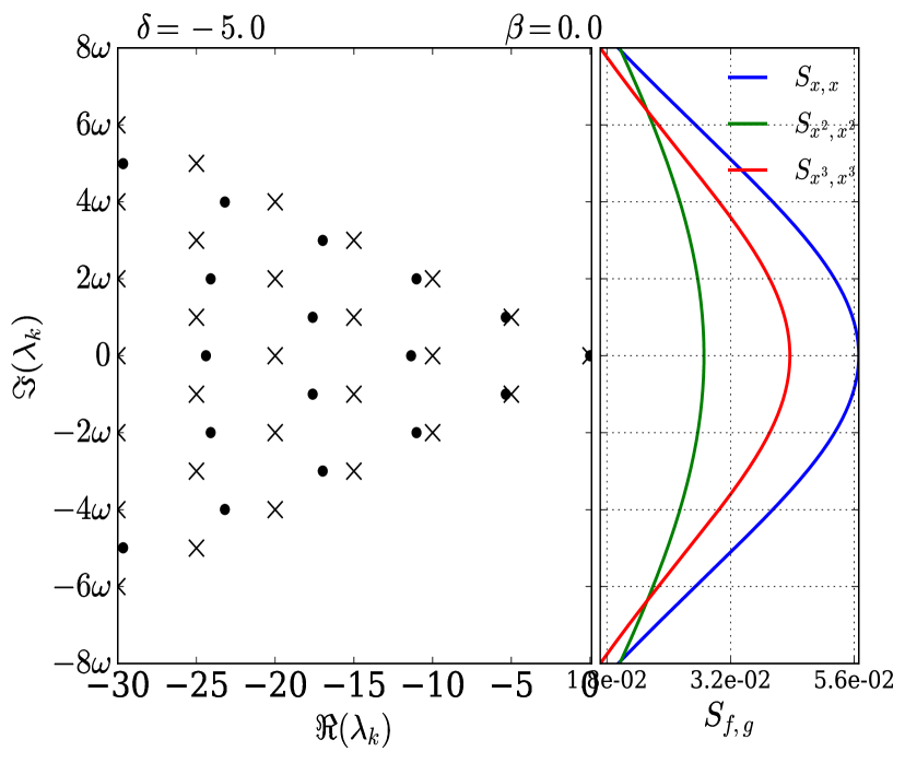
(a)

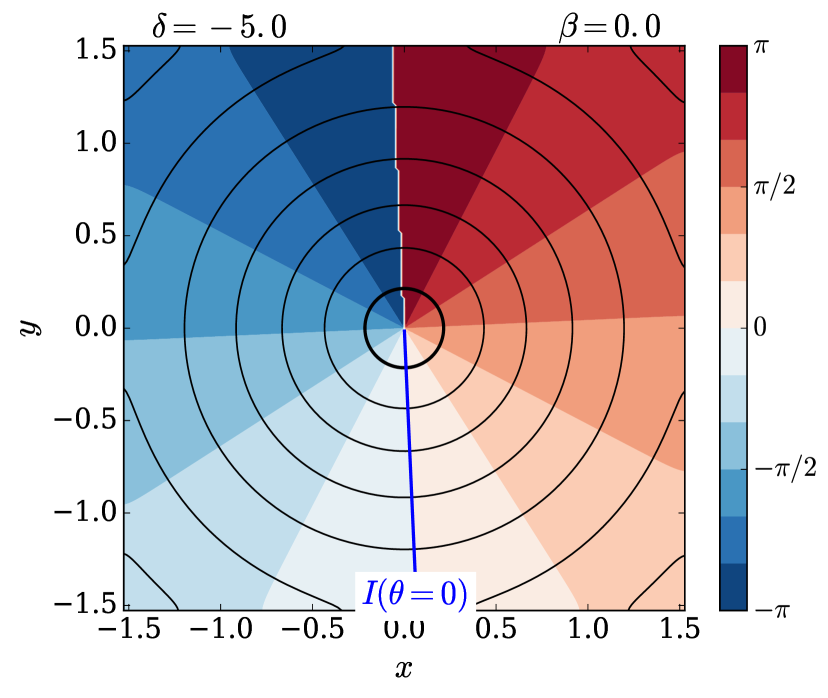
(b)

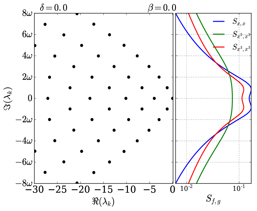
(c)

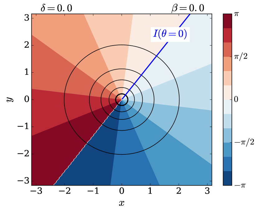
(d)

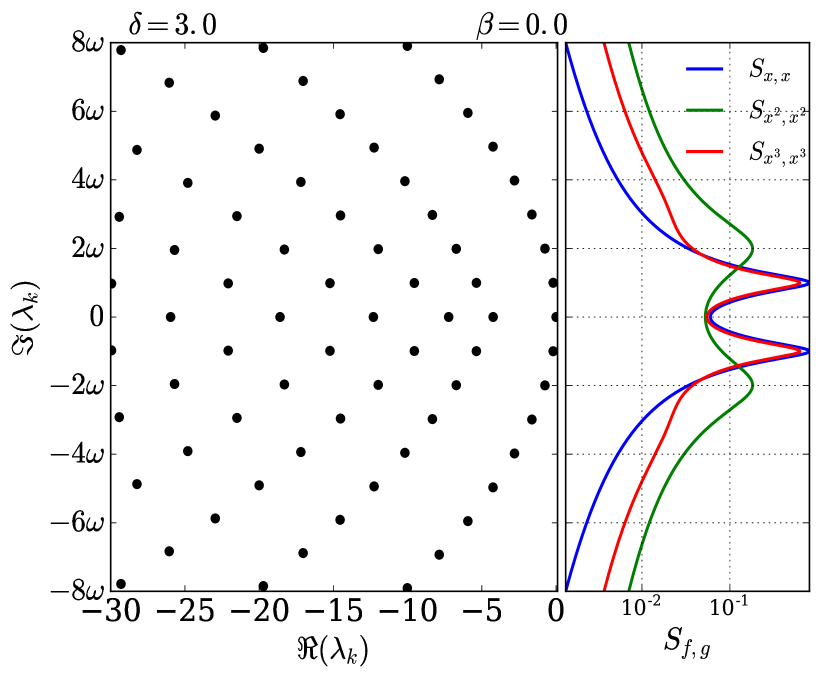
(e)

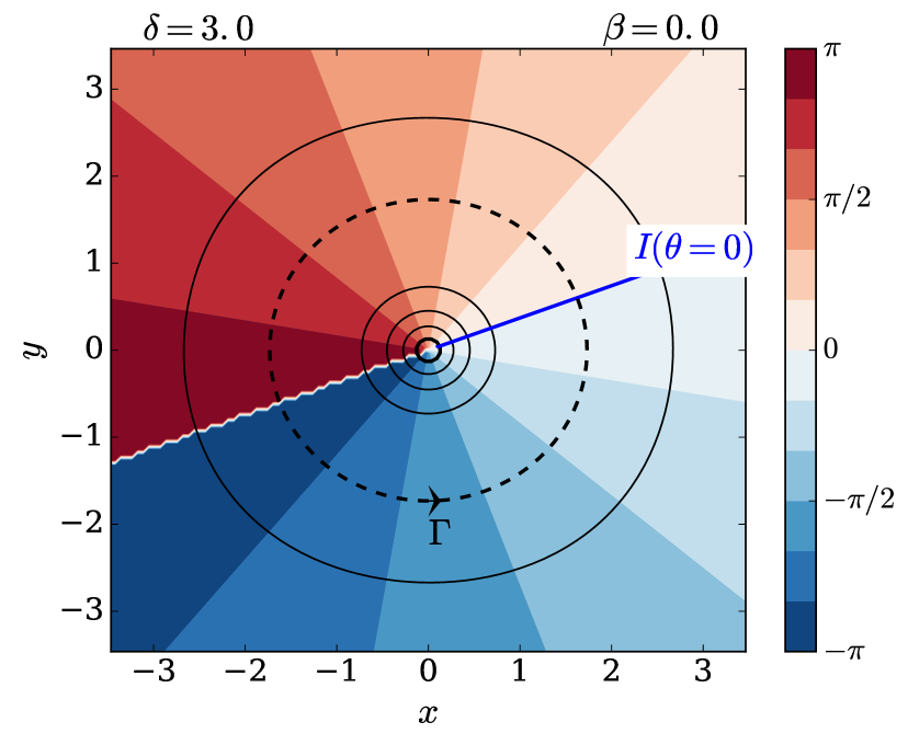
(f)

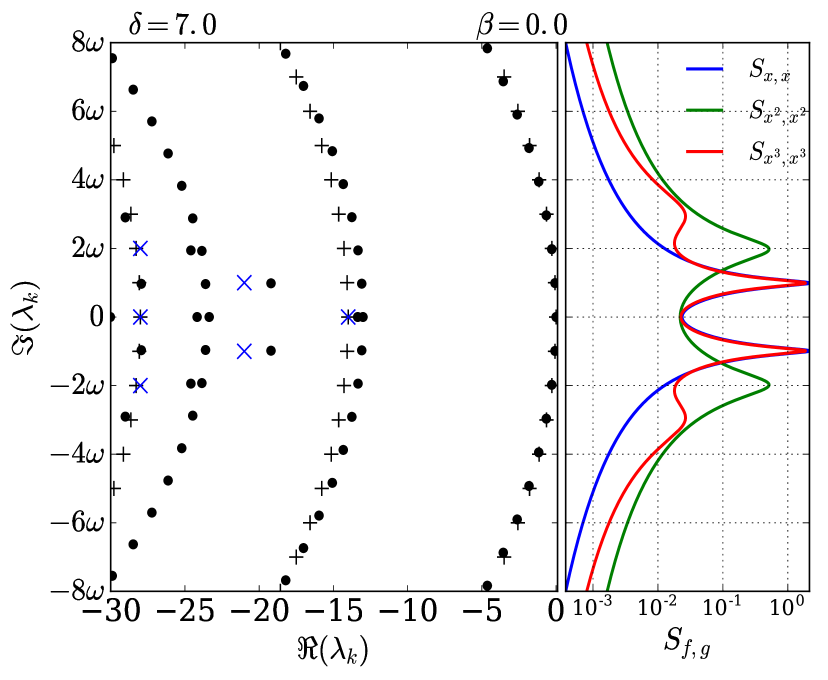
(g)

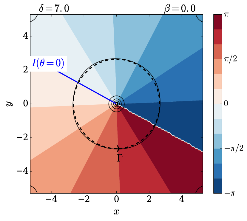
(h)

Figure 5: Left: Numerical approximation of the leading eigenvalues (black dots) of the Kolmogorov operator $\mathcal{K}$ for $\tilde{\beta}=0$, $\gamma=\kappa=1$ and (a) $\delta=-5$, (c) $\delta=0$, (e) $\delta=3$ and (g) $\delta=7$. In addition, the small noise prediction (4.2), for the RP resonances of the stable fixed point, is also represented as black crosses in panel (a). In (g), the small noise predictions (4.6, 4.7), for the eigenvalues of the unstable fixed point and of the limit cycle are also represented as blue crosses and black pluses, respectively. On the same panels, to the right, the power spectra between the three monomials $x$, $x^{2}$ and $x^{3}$ of the $x$ coordinate are also represented as blue, green and red lines, respectively (end of caption on next page). Right: Eigenfunction associated with the second eigenvalue with positive imaginary part. The phase of the eigenfunction is represented by filled contours and its amplitude by contour lines $(\mathbb{0.001},0.002,...)$.

We start by analyzing the numerical results for a fixed value of the noise level $\epsilon=1$ and a vanishing twist factor $\tilde{\beta}=0$, but different values of the control parameter $\delta$. In Fig. 5, the leading eigenvalues of the finite-difference approximation of the Kolmogorov operator $\mathcal{K}$ are represented as black dots on the left panels for (a) $\delta=-5$, (c) $\delta=0$, (e) $\delta=3$ and (g) $\delta=7$. In addition, the small noise prediction (4.2), for the RP resonances of the stable fixed point, is also represented as black crosses in panel Fig. 5-(a). In Fig. 5-(g), the small noise predictions (4.6), (4.7), for the eigenvalues of the unstable fixed point and of the limit cycle are also represented as blue crosses and black pluses, respectively. On the same panels, to the right, the power spectra between the three monomials $x$, $x^{2}$ and $x^{3}$ of the $x=r\cos\theta$ coordinate are also represented as blue, green and red lines, respectively. According to the order of the harmonics in the small-noise expansions (4.3) and (4.8) for the eigenfunctions and adjoint eigenfunctions, the observable $x$ is expected to project mainly on the eigenfunctions of the first complex pair of eigenvalues, $x^{2}$ on the eigenfunctions of the second pair and $x^{3}$ on the eigenfunctions of both the first and the third pair. These power spectra are calculated from the numerical approximations of the eigenvalues, eigenfunctions and adjoint eigenfunctions (i.e. the eigenvectors of the transpose of the finite-difference approximation of $\mathcal{K}$) according to the spectral decomposition (1.7). Finally, on the right panels, the corresponding eigenvector associated with the second eigenvalue with positive imaginary part represented . The phase of the eigenvectors is represented by filled contours and their amplitude by contour lines $(\mathbb{0.001},0.002,...)$.

For a small value of $\delta$, panel (a) of Fig. 5, a triangular structure of eigenvalues is found and, because of the large gap between the eigenvalues and the imaginary axis, the power spectra are broad, with no distinct resonance. The leading eigenvalues are in quantitative agreement with the small-noise expansion (4.2) around the stable fixed point represented in Fig. 4-(c). The corresponding second eigenfunction in panel (b) of Fig. 5 also agrees with the expansion $\psi_{01}$ of (4.3) represented in Fig. 4-(e). On the other hand, the secondary columns of eigenvalues are farther from the imaginary axis than the small-noise expansions. Since the numerical results have converged, this must be due to higher-order terms in the expansions which are not taken into account and which can depend on the noise level $\epsilon$ and be responsible for more mixing. This points at the fact that, in the expansion (4.2), we do not control the weight of the higher-order terms in $\epsilon^{2}$ as we switch from one eigenvalue to the next. One should thus take this effect into account when the noise level is strong with respect to the contraction measured by $\delta$. This is particularly important when considering eigenvalues farther from the imaginary axis. Indeed, the latter typically exhibit more complex nodal properties, as is the case in the small-noise expansion (4.3) and in general for multi-dimensional Ornstein-Uhlenbeck processes for which the eigenfunctions are polynomials of increasing degree MPP (02), and are thus more difficult to approximate (Var, 71, see e.g.).

As the control parameter $\delta$ is increased (from panel (a) to (c) in Fig. 5) the eigenvalues get closer to the imaginary axis, as expected from the weaker stability of the limit cycle and as predicted by the expansion (4.2) for the stable fixed point. One can also see from the larger gaps between the contour lines in Fig. 5-(d) compared to those of Fig. 5-(b) that the amplitude of the second eigenvector flattens, in agreement with (4.3). Because of the approach of the first complex pair of eigenvalues to the imaginary axis, in agreement with the spectral decomposition (1.7) and the eigenfunction expansions (4.3, 4.8), broad peaks begin to appear in the power spectra of the observables $x$ and $x^{3}$ at angular frequencies given by the imaginary part of the eigenvalues. On the other hand, the second pair is still too far for the observable $x^{2}$ to resonate.

As $\delta$ is further increased (panels (c-d) to (g-h) of Fig. 5) and the bifurcation point is crossed, a rather smooth transition from the small-noise expansions for $\delta>0$ and then $\delta<0$ occurs, in which the first line of eigenvalues gets closer and closer to the imaginary axis. As a result, strong resonant behavior occurs for all three observables, as can be seen from the sharpening of the spectral peaks at the position of the first three harmonics. The peaks remain finite, however, since, in agreement with the small-noise expansion (4.7), a spectral gap persists between the eigenvalues and the imaginary axis, due to the noise. Finally, for $\delta=7$ inn panel Fig. 5-(g), one finds the superposition of a family of parabolas and of a triangular family of eigenvalues, in very good agreement with the small-noise expansions (4.7) and (4.6) for the limit cycle and for the unstable fixed point, respectively, while the corresponding eigenvector on panel Fig. 5-(h) has an almost uniform amplitude, in agreement with (4.8), except at the origin (c.f. Fig. 4-(d, f)).

In agreement with the results of Section 3, the spectrum remains discrete during the transition, as opposed to the deterministic case (c.f. GT (01)). On the other hand, precisely how the transition occurs could not be predicted analytically from the geometric properties of the deterministic flow. In particular, eigenvalues farther away from the real axis tend to approach the imaginary axis at a faster rate than the others, resulting in a curving of the triangle array of eigenvalues, while the second eigenvector continues to flatten away from the origin. Eventually (from panel Fig. 5-(e) to Fig. 5-(g)), parabolas of eigenvalues detach one after the other, while other eigenvalues persist as a triangular family.

So far, these numerical experiments have mostly allowed to test the validity of the small-noise expansions of Section 4 when the twist factor $\tilde{\beta}$ is vanishing and to reveal unpredicted phenomena close to the bifurcation point. Next, the role of $\tilde{\beta}$ is investigated and a more detailed numerical analysis of the change of the RP spectrum close to the bifurcation point is given.

5.2.2 Crossing the bifurcation point, with a nonzero twist factor

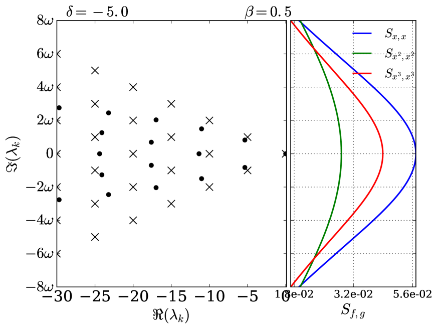
(a)

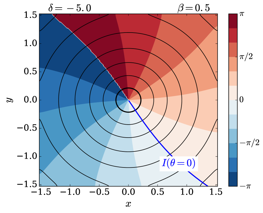
(b)

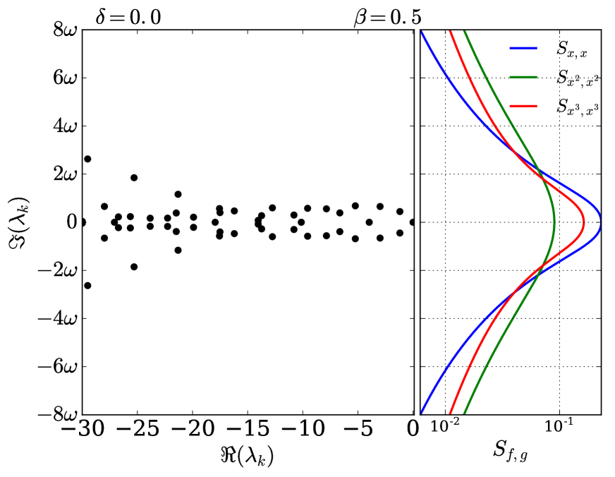
(c)

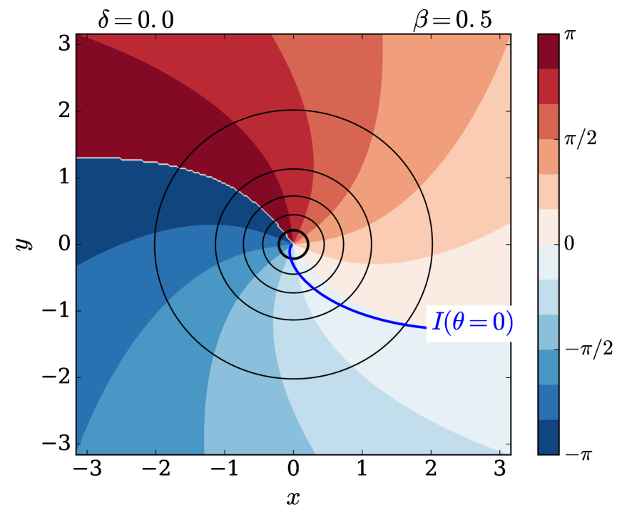
(d)

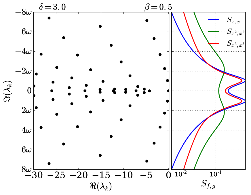
(e)

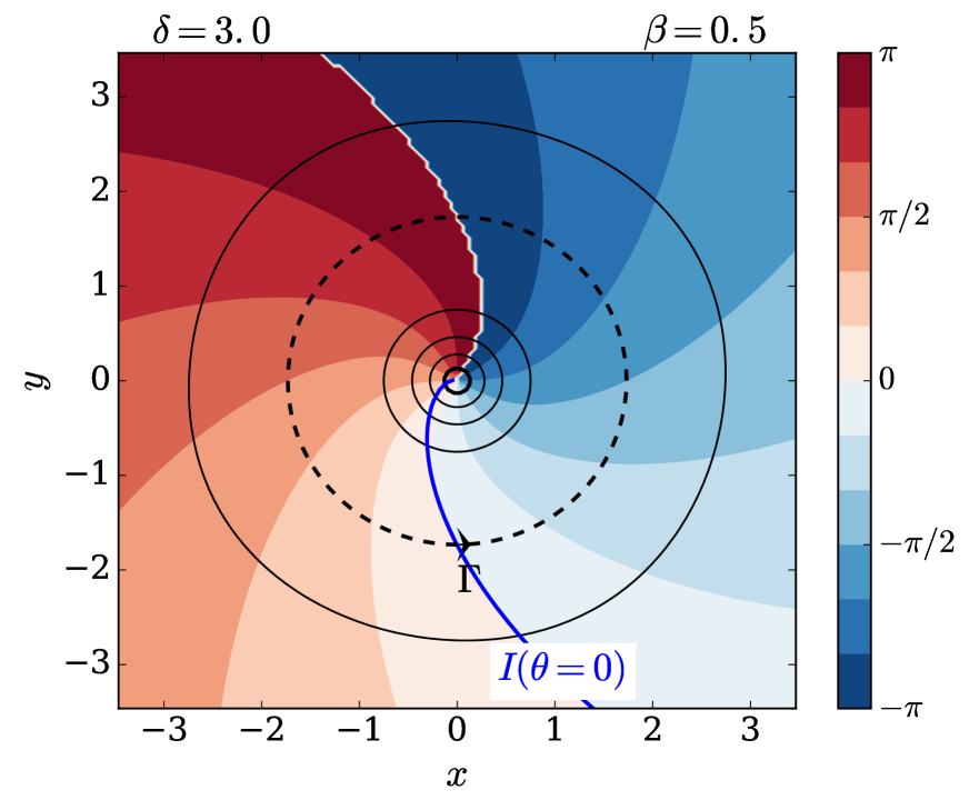
(f)

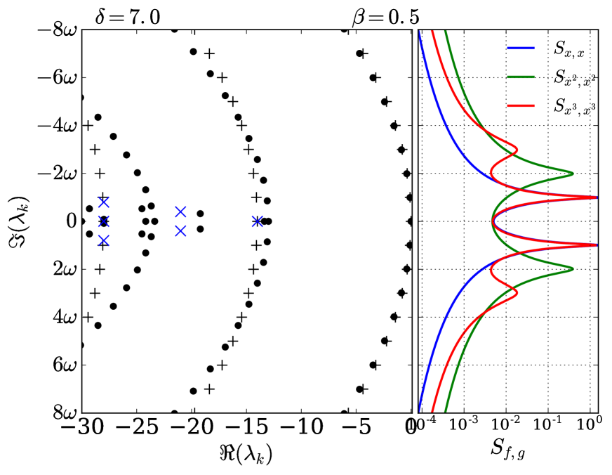
(g)

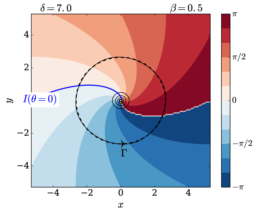
(h)

Figure 6: Same as Fig. 5 but with $\tilde{\beta}=0.5$.

To learn more about the change in the spectrum when the twist factor $\tilde{\beta}$ is nonzero, the same set of numerical experiments as in the previous subsection 5.2.1 is performed, but with $\tilde{\beta}=0.5>0$. The results are reported in Fig. 6 in the same way as in Fig. 5. Below the bifurcation point, the small-noise expansions (4.2) and (4.3) do not depend on $\tilde{\beta}$, so that panels (a) and (b) of Fig. 5 and 6 should be identical. As closer inspection shows this is not exactly the case, so that the noise level is strong enough to excite higher-order terms in $\epsilon$ which depend on $\tilde{\beta}$, in agreement with the $\mathcal{O}_{\tilde{\beta}}$ in the expansions of Proposition 4 and 5. As a result, the imaginary parts of the eigenvalues are smaller, due the decrease of the frequency of the fundamental and its harmonics induced by the twist factor $\tilde{\beta}$. In addition, the isolines of phase of the second eigenvector (panel (b) of Fig. 6) are slightly tilted. One discerns on panels (c) and (d) of Fig. 6 that both effects become more prominent closer to the bifurcation point, i.e. the eigenvalues are even closer to the real axis and the isolines of phase even more tilted. In particular the fact that the eigenvalues get closer to the real axis, and even cross it, results in a dramatic change in the power spectra where the resonances are much more centred, so that no spectral peak is visible away from $0$ in Fig. 6-(c).

On the other hand, one distinguishes on panels (g) and (h) of Fig. 6 that the small-noise expansions (4.6), (4.7) and (4.8) are in very good agreement with the numerical results far above the bifurcation point. In particular, the increase of the spectral gap associated with the increase of the phase diffusion due to the nonzero twist factor $\tilde{\beta}$ as well as the tilt of the isolines of phase of the second eigenvector with the isochrons are captured. To summarize, the twist factor $\tilde{\beta}$ is responsible for increasing the mixing, changing the position of the harmonics and twisting the eigenvectors.

5.2.3 Parameter dependence close to bifurcation

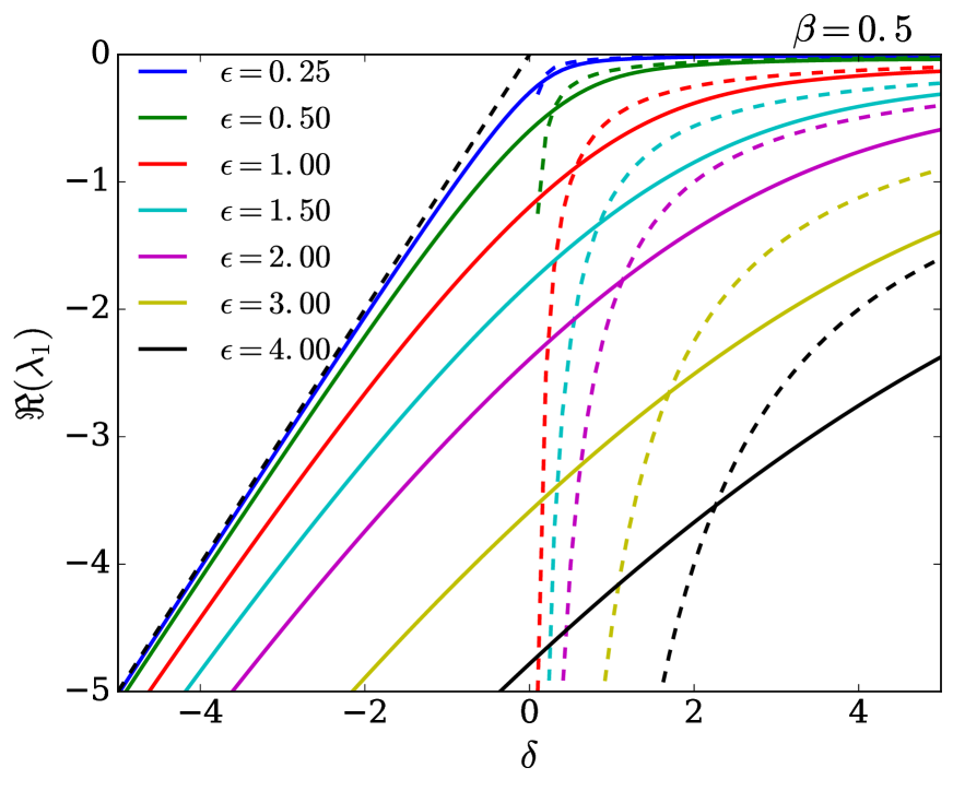
(a)

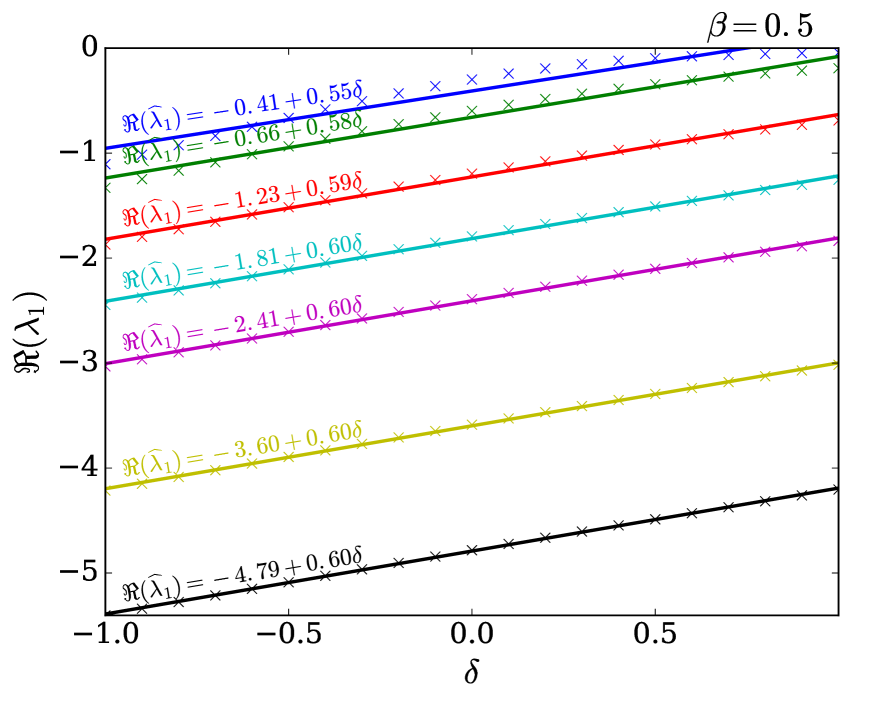
(b)

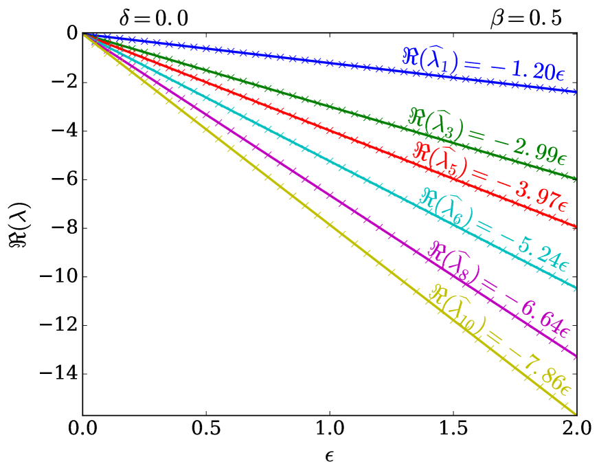
(c)

Figure 7: Top left: Real part of the approximated second eigenvalue $\lambda_{1}$ versus $\delta$ for $\tilde{\beta}=0.5$ (thick lines) and with $\gamma=\kappa=1$. Different colors correspond to different values of the noise level $\epsilon$ (see the legend). For $\delta<0$, the curve $\Re(\lambda_{1})=\delta$ corresponding to the small-noise expansion (4.2) is plotted as a dashed black line. For $\delta>0$, the curves $\Re(\lambda_{1})=-\epsilon^{2}(1+\tilde{\beta}^{2})/(2R^{2})$ corresponding to the small-noise expansion (4.7) are plotted as dashed lines in the color corresponding that of the numerical approximation for a given $\epsilon$.
Top right: Zoom to $\delta$ in the interval $[-1,1]$. The numerical approximations are now represented as crosses in the same color as on the right together with a least-square fit of the line $y=a+b\delta$.
Bottom: Real part of the approximated leading eigenvalues versus he noise level $\epsilon$ for $\delta=0$ (crosses). The lines represent least square fits $y=a+b\epsilon$.

In order to better understand the parameter dependence of the RP spectrum close to bifurcation, we focus now on the real part of the second eigenvalue $\lambda_{1}$. Its numerical approximation is represented in Fig. 7 for varying $\delta$ and $\epsilon$ with fixed $\tilde{\beta}=0.5$. On the left panel, each line corresponds to the numerical approximation of $\Re(\lambda_{1})$ for different values of the noise level $\epsilon$ (color code in the legend). In addition, the dashed black line $\Re(\lambda_{1})=\delta$ corresponds to the small-noise expansion (4.2) for $\delta<0$ and the colored dashed lines $\Re(\lambda_{1})=-\epsilon^{2}(1+\tilde{\beta}^{2})/(2R^{2})$ correspond to the small-noise expansion (4.7) for $\delta>0$ and different values of $\epsilon$. As expected, for smaller values of $\epsilon$ and larger absolute values of $\delta$, the numerical approximations converge to the small-noise expansions. On the other hand, strong deviations occur when the noise level is increased or when the system is placed closer to the bifurcation point. There, the eigenvalue transits smoothly from the small-noise expansions for $\delta<0$ to $\delta>0$. Interestingly, this change occurs more slowly when $\epsilon$ is large, so that the noise has a stabilizing effect on the dependence of the eigenvalue of $\delta$.

On the right panel of Fig. 7, a zoom to $\delta\in[-1,1]$ allows for a more detailed analysis of the changes in the second eigenvalue. There, the numerical approximations of $\Re(\lambda_{1})$ are represented by crosses in the same colors as the left panel for the same values of $\epsilon$. On top of them is plotted their least-square fit of the line $y=a+b\delta$. Interestingly, the linear regressions performs very well for a range of $\delta$’s values close to $0$, the latter increasing with $\epsilon$. Even more surprising, the slope of the linear regressions does not seem to depend on the noise level $\epsilon$. In other words, the dependence of the minimum decay rate of correlations $\Re(\lambda_{1})$ on the control parameter $\delta$ around $0$ is close to linear, on a range which increases with the noise level $\epsilon$ but with a coefficient which does not depend on $\epsilon$.

To learn more about the role of the noise for $\delta=0$, the approximation of the real part of the leading eigenvalues versus $\epsilon$ are represented on the bottom panel of Fig. 7 by crosses. Least square fits $y=a+b\epsilon$ are also represented by lines. In agreement with the scaling relationship (5.1), all real parts depend linearly on $\epsilon$. Yet, it is interesting to see that the slope of the lines is steeper for higher-rank eigenvalues, farther from the imaginary axis. In other words, eigenvalues farther from the imaginary axis are more sensitive to the noise, so that, as the noise level is increased, they move away from the imaginary axis at a faster rate.

(a)

(b)

Figure 8: Left: Real part of the finite-difference approximation of the second RP resonance $\lambda_{1}$ versus $\delta$ (thick lines), for $\epsilon=0.25$ (blue), $\epsilon=0.5$ (green), $\epsilon=1$ (red), $\epsilon=1.5$ (cyan), $\epsilon=2$ (magenta). For $\delta>0$, the small-noise curves $\Re(\lambda_{1})=-\epsilon^{2}/(2\delta)$ are plotted as dashed lines in the corresponding color. For $\delta<0$, the small noise curve $\Re(\lambda_{1})=\delta$ is plotted as a black dashed line.
Right: Real part of the finite-difference approximation of the second RP resonance $\lambda_{1}$ versus $\epsilon$, for $\delta=0$ (plus) and $\delta=5$ (cross). For $\delta=0$, the least-square linear regression with coefficient $-1.18$ is also represented as a dashed line. For $\delta=0$, the curve $\Re(\lambda_{1})=-\epsilon^{2}/(2\delta)$ is also represented as dotted dashed line.

Finally, we investigate the dependence of the RP spectrum on $\tilde{\beta}$ at the bifurcation point. In Fig. 8 is represented by crosses the evolution of the real parts (left panel) and imaginary parts (right panel) of the approximated leading eigenvalues, for $\delta=0$ and $\epsilon=1$. On top of the real parts on the left are also represented the least square fits $y=a+b\tilde{\beta}^{2}$. Their perfect match reveals the quadratic dependence of the real parts of the leading eigenvalues on $\tilde{\beta}$, as is also the case for the small-noise expansions (4.7) for $\delta>0$. This dependence is, however not uniform, as the real part of some eigenvalues are more sensitive to $\tilde{\beta}$ than others. Second, the perfect match of the least square fits $y=a+b\epsilon$ on the imaginary parts (right panel) reveals their linear dependence on $\tilde{\beta}$. Moreover, this dependence is much stronger for eigenvalues initially farther from the real axis when $\tilde{\beta}=0$. This result is in agreement with the strong folding of the high harmonics from one side of the real axis to the other in Fig. 6-(c) and Fig. 6-(d).

6 Summary and Discussion

We examined the stochastic Hopf bifurcation from the perspective of the Markov semigroup and the spectrum of its generator. The latter—the RP spectrum—provides a characterization of the dynamics, permitting among other things a decomposition of the correlation functions and related power spectra; see (CTND, 20, Corollary 1 and Sec. 2.3). Contrary to the traditional characterization of a bifurcation in terms of crossing of the imaginary axis by the eigenvalues of the linearized problem, the RP resonances have real parts that remain negative as one crosses the criticality. Bifurcations are instead characterized by a change in the geometric patterns formed by the RP spectrum in the left half complex plane, and in particular the decay of correlations. The RP spectrum allows for a unifying framework of stochastic analysis and Fokker-Planck equations relevant and useful for the study of stochastic bifurcations. For instance, the stochastic analysis techniques reviewed in CTND (20) and related decomposition formulas of correlations and power spectra, are applied here to the Hopf bifurcation case and small-noise expansions are derived for the corresponding eigenvalues and eigenfunctions in terms of an adimensional small parameter involving the noise level and the coefficients controlling the stability of the deterministic solutions.

As in the deterministic case, weak values of the parameter $\delta$ controlling the distance to the deterministic bifurcation point are associated with the slowing down of the decay of correlations, as given by the gap between the leading RP resonances and the imaginary axis; see Section 4. However, the application, in Section 3, of the theory of Lyapunov functions and ultimate bounds (see (CTND, 20, Theorems 5 & 6)) allows us to show that noise implies the existence of a spectral gap that stays away from zero, even at and above the bifurcation point, leading to correlations that always decay exponentially. In particular, while above the bifurcation point the neutral deterministic dynamics on the limit cycle is associated with purely imaginary eigenvalues and is thus non-mixing, phase diffusion due to the noise ensures mixing along this limit cycle as well as the existence of a stationary density. This phase diffusion results in the characteristic parabolic structure of the RP resonances above the bifurcation point (4.7), as opposed to the triangular one below this point (see (4.2)), in the small-noise case considered in Sec. 4.

To understand this phase diffusion, we use the concept of isochrons provided by the set of points that share the same asymptotic phase, on the limit cycle. This allows us to derive an SDE for the phase evolution in which two contributions appear: one coming directly from the azimuthal direction, and one resulting from the interaction of the deterministic vector field with the radial noise; see Eq. (2.21). This interaction is quantified thanks to the Hörmander condition which in terms of isochrons can be summarized as (see Theorem 1 and Fig. 3):

For phase diffusion to occur, it is necessary that at least one component of the noise acts transverse to the isochrons.

In particular, even if the stochastic vector field is tangent to the radial direction, phase diffusion can occur as long as the isochrons are transverse to this direction. In the case of the stochastic Hopf bifurcation considered here, it was shown in Section 2 that the tilt of the isochrons is controlled by the twist factor $\tilde{\beta}=\beta/\kappa$ measuring the dependence of the frequency of the oscillations on their amplitude. This effect was directly visible from the isolines of phase of the RP eigenfunctions obtained in Section 4, in the small-noise case, as well as in the phase diffusion coefficient $\epsilon^{2}(1+(\beta/\kappa)^{2})/R^{2}$ entering the real parts of the small-noise expansion about the limit cycle of the RP resonances. These formulas for the resonances are particularly useful, as they allow one to quantitatively relate the phenomenon of phase diffusion to the broadening of the peaks in the power spectrum.

While, in the general case of a hyperbolic limit cycle in the presence of noise, the tilt of the isochrons with respect to the stochastic forcing can in principle be measured, no single parameter playing the role of twist factor can in general be singled out. In addition, the calculation, even numerical, of the global isochrons of a high-dimensional system is a difficult task. However, in the small-noise case, only local information on the isochrons about the limit cycle is necessary. Indeed, it was shown by Gas (02) that the effect of the interaction of the noise with the deterministic vector field integrated over one period of the limit cycle is measured by the coefficient

$$\Phi=-\frac{\epsilon^{2}\omega_{f}^{2}}{T}\frac{\left<C(T)\vec{f}^{R}_{2},\vec{f}^{R}_{2}\right>}{\left<\vec{e}^{R}_{2},\vec{f}^{R}_{2}\right>},$$ (6.1)

where $\epsilon$ is the noise level and $\vec{e}^{R}_{2}$ and $\vec{f}^{R}_{2}$ are respectively the right and left eigenvectors of the matrix $R$ of the Floquet representation (A.7) of the fundamental matrix $M(t)$ associated with the eigenvalue $0$ (care should be taken to normalize $\vec{e}^{R}_{2}$ to the same magnitude of the vector field for (6.1) to be valid) ; see Section 2.3. The matrix $C(t)$ is given by

$$C(t) =\int_{0}^{t}M(t)M(-s)D_{\Gamma}(s)(M(t)M(-s))^{*}ds$$ (6.2)

and corresponds to the correlation matrix DL (95); GL (08) of a periodic Ornstein-Uhlenbeck process with a drift given by the Jacobian matrix $A(t)$ (see Appendix (A.1)) and with a diffusion matrix $D_{\Gamma}(t)$, both evaluated along the limit cycle. A simple calculation, given in Appendix A.1, shows that, in the case of the stochastic Hopf bifurcation considered here, the coefficient $\Phi$ correctly coincides with the diffusion coefficient entering the real parts of the small-noise expansion about the limit cycle of the RP resonances. Thus, in the small-noise case, the phase diffusion coefficient (6.1) is readily accessible from the local properties of the deterministic system about the limit cycle.

From the difference in structure of the RP spectrum below and above the bifurcation point identified in Section 4, one could hope to distinguish the case of a single stable stationary point perturbed by noise below the bifurcation, from the case of a perturbed limit cycle above the bifurcation. However, close to the bifurcation point and for a high level of noise, the small-noise expansions of the eigenvalues are no longer in agreement with the numerical approximations of Section 5. The stochastic dynamics can no longer be understood in terms of small perturbations of the deterministic dynamics. The numerical approximations, however, give evidence that new constraints emerge at the bifurcation point. These results can be summarized as follows:

• The numerical approximations are in good agreement with the small-noise expansions of Section 4 far from the bifurcation point and for a small noise-level, even though eigenvalues farther from the imaginary axis tend to be more sensitive to the truncation. • As the bifurcation point is crossed, a transition occurs from a triangular structure of eigenvalues to a parabolic one and the eigenvalues remain discrete. • For $\delta\approx 0$, there is a $\delta$-interval over which the real parts of the eigenvalues are to a large extent linearly dependent on the bifurcation parameter $\delta$. This interval widens with the noise level, but the slope does not depend on it. • For $\delta=0$, the real parts of the eigenvalues depend linearly on the noise, but eigenvalues farther from the imaginary axis are more sensitive to the noise. • The effect of the twist factor $\tilde{\beta}=\beta/\kappa$ on the RP eigenfunctions and eigenvalues is already visible below the bifurcation point. • For $\delta=0$, the real parts and the imaginary parts of the leading eigenvalues depend quadratically and linearly on the twist factor $\tilde{\beta}$, respectively. • Eigenvalues that would correspond to higher harmonics for $\tilde{\beta}=0$ can evolve rapidly with changes in $\tilde{\beta}$ and $\delta$ and need not correspond to integer multiples of a constant fundamental frequency. This is particularly noticeable near the bifurcation and can have subtle consequences for the power spectrum.

The geometric characterization of the phenomenon of phase diffusion and the formulas for the RP eigenvalues and eigenfunctions allow one to gain novel insights on the dependence of the regularity of nonlinear oscillators forced by noise not only on the noise level, but also on the stability of the underlying limit cycle and on the twist of its isochrons.

The analysis conducted here on the stochastic Hopf equation points out a rich set of properties that builds intuition for examination of more complex nonlinear oscillations in presence of noise. In the third part of this contribution TCND (19), these results are applied to models of a leading mode of climate variability, El Niño-Southern Oscillation, for which understanding the dynamics behind its aperiodicity remains a challenge.

Appendix A Floquet theory applied to the Hopf normal form

Floquet theory allows one to characterize the local stability properties of deterministic flows about a periodic orbit. These properties are essential to the response of the system to stochastic forcing studied in Section 3 and to the small-noise expansions of the RP spectrum obtained in Section 4. We thus review here standard results from the application of Floquet theory to the normal form (2.1) of the Hopf bifurcation.

Small deviations $x^{\prime}(t)$ from the orbit $x_{\Gamma}(t)$ associated with the limit cycle $\Gamma$, satisfy the variational equation (Kuz (98), Chap. 1.5)

$$\dot{x^{\prime}}(t)=A(t)x^{\prime}(t),\quad x^{\prime}(t)\in{\color[rgb]{0,0,0}\mathbb{R}^{2}},\quad t\in\mathbb{R}.$$ (A.1)

Here, $A(t):=(DF)_{x_{\Gamma}(t)}$ denotes the Jacobian matrix about the orbit $x_{\Gamma}(t)$, of the vector field $F$ associated with the Hopf normal form written in Cartesian coordinates, i.e. the RHS of Eq. (2.6) for $\epsilon=0$. In other words, $A(t)$ provides the tangent map of $F$ along $x_{\Gamma}(t)$. Thus, $A$ is periodic, i.e., $A(t+T)=A(t)$, for any $t$ in $\mathbb{R}$. Let $M(t)$ be a fundamental solution (Har (64), Chap. IV.1) of (A.1), i.e.,

$$\dot{M}(t)=A(t)M(t)\quad\mathrm{and~{}}\det M(t)\neq 0,\quad t\in\mathbb{R}.$$ (A.2)

Then the Floquet theorem (e.g. Har (64), Theorem IV.6.1) ensures that $M(t)$ has the following representation

$$M(t)=Z(t)e^{tR},\quad\mathrm{where~{}}Z(t+T)=Z(t),\quad t\in\mathbb{R},$$ (A.3)

and $R$ is a constant matrix. Imposing, without loss of generality, that $M(0)=I$ yields $Z(T)=Z(0)=I$ and $M(T)=e^{TR}$.

While determining the Floquet representation of a fundamental matrix is in general a difficult task, in the case of the Hopf normal form (2.1), it can easily be found from the linearization of the vector field in polar coordinates. In that respect, we assume furthermore that $\delta$ in Eq. (2.1) is positive. The orbit $x_{\Gamma}(t)$ writes then $(R,\theta_{0}+\omega_{f}t)$, for some initial phase $\theta_{0}$. The linearization about $\Gamma$ of the vector field (2.14) in polar coordinates is given by the matrix

$$J_{\Gamma}(t)=\begin{pmatrix}-2\delta&0\\ -2\beta R&0\end{pmatrix}$$ (A.4)

and depends implicitely on time only through the evolution of the tangent space on which it acts with the reference solution $x_{\Gamma}(t)$, so that the time argument will be dropped in the sequel.

To proceed, let us introduce the Jacobian matrix of the transformation $(x,y)\to(r,\theta)$ and its inverse, respectively given by

$$J_{\mathrm{polar}}(r,\theta) =\begin{pmatrix}\cos\theta&\sin\theta\\ -r^{-1}\sin\theta&r^{-1}\cos\theta\end{pmatrix}=~{}S^{-1}(r)L(-\theta),\quad r>0$$

$$J_{\mathrm{polar}}^{-1}(r,\theta) =\begin{pmatrix}\cos\theta&-r\sin\theta\\ \sin\theta&r\cos\theta\end{pmatrix}=~{}L(\theta)S(r),$$

where we have used the rotation and diagonal matrices

$$L(\theta)=\begin{pmatrix}\cos\theta&-\sin\theta\\ \sin\theta&\cos\theta\end{pmatrix}\quad\mathrm{and}\quad S(r)=\begin{pmatrix}1&0\\ 0&r\\ \end{pmatrix}.$$

The matrix $J_{\Gamma}$ is then related to the matrix $A(t)$ of the tangent map $(DF)_{x_{\Gamma}(t)}$ in Cartesian coordinates by

$$A(t)=J_{\mathrm{polar}}^{-1}(R,\theta_{0}+\omega_{f}t)~{}J_{\Gamma}~{}J_{\mathrm{polar}}(R,\theta_{0})+\omega_{f}L(\frac{\pi}{2}),\quad t\in\mathbb{R}.$$ (A.5)

That the conversion of $J_{\Gamma}$ to Cartesian coordinates coincides with the matrix $A(t)$ of the tangent map but for the term $\omega_{f}L(\pi/2)$ is due to the rotation of the polar frame along the limit cycle $\Gamma$, which was not taken into account when calculating $J_{\Gamma}$.

One can then verify that the matrix

$$M(t)=J_{\mathrm{polar}}^{-1}(R,\theta_{0}+\omega_{f}t)~{}e^{tJ_{\Gamma}}~{}J_{\mathrm{polar}}(R,\theta_{0}),\quad t\in\mathbb{R},$$ (A.6)

is a solution to (A.2), for the reference solution $x_{\Gamma}(t)$ on $\Gamma$. Since

$${\color[rgb]{0,0,0}J_{\mathrm{polar}}^{-1}(R,\theta_{0}+\omega_{f}t)=L(\omega_{f}t)~{}J_{\mathrm{polar}}^{-1}(R,\theta_{0}),}$$

it follows that the fundamental matrix $M(t)$ has a Floquet representation

$$M(t)=Z(t)~{}e^{tR},\quad t\in\mathbb{R},$$ (A.7)

$$\mathrm{with}\enskip Z(t)=L(\omega_{f}t)\quad \mathrm{and}\enskip R=J_{\mathrm{polar}}^{-1}(R,\theta_{0})~{}J_{\Gamma}~{}J_{\mathrm{polar}}(R,\theta_{0}).$$

Applying $M(t)$ to a vector $x^{\prime}$ at time $0$ thus corresponds to converting this vector to polar coordinates, integrating to a time $t$ according to the generator $J_{\Gamma}$ and converting back from polar coordinates at time $t$. In other words, the polar frame at $x_{\Gamma}(t)=(R,\theta_{0}+\omega_{f}t)$ constitutes a co-moving frame adapted to the Floquet representation of $M(t)$.

Note next that $J_{\Gamma}$ can be diagonalized as

$$J_{\Gamma}=E~{}\Lambda~{}F^{*}$$ (A.8)

$$\mathrm{with}~{}E=\begin{pmatrix}1&0\\ \frac{\tilde{\beta}}{R}&1\end{pmatrix},\quad \Lambda=\begin{pmatrix}-2\delta&0\\ 0&0\end{pmatrix}\quad\mathrm{and}\quad F^{*}=E^{-1}=\begin{pmatrix}1&0\\ -\frac{\tilde{\beta}}{R}&1\end{pmatrix},$$

where $F^{*}$ denotes the complex conjugate of the matrix $F$. Then, from the definition (A.7) of $R$,

$$R=E_{R}~{}\Lambda~{}F_{R}^{*}$$ (A.9)

$$\mathrm{with}~{}E_{R}=J_{\mathrm{polar}}^{-1}(R,\theta_{0})~{}E\quad \mathrm{and}\quad F^{*}_{R}=E_{R}^{-1}=F^{*}~{}J_{\mathrm{polar}}(R,\theta_{0}).$$

Thus, the eigenvalues of $R$ coincide with those of $J_{\Gamma}$ and its eigenvectors are given by converting those of $J_{\Gamma}$ from polar coordinates.

The eigenvalues $\alpha_{1}$ and $\alpha_{2}$ of $R$ are called the characteristic exponents of $\Gamma$ and the eigenvalues of $e^{TR}$ its characteristic multipliers (GH (83), Chap. 1.5). The eigenvector associated with $\alpha_{2}$ is in the direction of the flow, so that $e^{T\alpha_{2}}$ is always unity. On the other hand, the other eigenvalue $\alpha_{1}=-2\delta$ determines the stability of the periodic orbit. It is in fact the eigenvalue of the tangent map $DS_{T}$ of the Poincaré map.

A.1 Calculation of the phase diffusion coefficient from the correlation matrix

In the case of the stochastic Hopf bifurcation considered here, the diffusion matrix $D_{\Gamma}$ in (6.2) for any point on $\Gamma$ is given in polar coordinates by

$$D_{\Gamma} =\begin{pmatrix}1&0\\ 0&\frac{1}{R^{2}}\end{pmatrix},\quad t\in\mathbb{R}$$ (A.10)

and is hence constant in time. Since $\vec{f}^{R}_{2}$ is a left eigenvector of the matrix $M(T)=e^{TR}$ with $R$ given by (A.7), it follows that

$$\Phi=-\epsilon^{2}\omega_{f}^{2}\left<D_{\Gamma}\vec{f}_{2},\vec{f}_{2}\right>=-\epsilon^{2}\frac{1+\tilde{\beta}^{2}}{R^{2}}=-\epsilon^{2}\frac{1+\beta^{2}}{\delta\kappa},$$ (A.11)

where $\vec{f}_{2}=\omega_{f}^{-1}(-\tilde{\beta}/R),1)$ is the conversion to polar coordinates of the left eigenvector $\vec{f}^{R}_{2}$ of $R$ and, according to (A.9), coincides with the left eigenvector of the polar Jacobian matrix $J_{\Gamma}$ in (2.15) at initial time. The factor $\omega_{f}^{-1}$ in $\vec{f}_{2}=(-\tilde{\beta}/(\omega_{f}R),1)$ is due to the normalization of $\vec{e}^{R}_{2}$ to the magnitude of the vector field $F$ on $\Gamma$, which is essential for (6.1) to hold.

Appendix B Proofs of the stochastic analysis results of Section 3

B.1 Proof of Theorem 1: isochrons and Hörmander condition

For two arbitrary smooth vector fields $V$ and $W$, recall that the Lie bracket $[V,W]$ coincides with the Lie derivative $\mathcal{L}_{V}W$ of $W$ along $V$. The Lie derivative can be defined in terms of pullback of a vector field by a diffeomorphism. The pullback, or Lie transport, $(S_{t}^{V*}W)(q)$ at a point $q$ of a vector field $W$ by the flow $S_{t}^{V}$ generated by $V$ can be defined as the vector at $q$ tangent to the image by $S_{-t}^{V}$ of any curve to which $W(S_{t}^{V}q)$ is tangent. The Lie derivative at a point $q$ is then defined in terms of pullback of a vector field, by

$$\mathcal{L}_{V}W=\and{\frac{\,\mathrm{d}}{\,\mathrm{d}t}}{0}S_{t}^{V*}W.$$ (B.1)

This expression says that $\mathcal{L}_{V}W$ measures the rate of change of $W$ due to the Lie transport (Fec, 06, Chap. 3-4). Note that the Lie derivative is well defined because both the vector field at some point and its pullback at the same point live in the tangent space to the manifold at this point. The following is derived from the fact that the isochrons are permuted by the flow $S_{t}$ generated by $V_{0}$ (Proposition 2-(ii)): if a vector field $V_{i}$ is tangent to an isochron $W_{ss}(S_{t}p)$ at some point $S_{t}q$, i.e. if $V_{i}(S_{t}q)\in TW_{ss}(S_{t}p)$, where $TW_{ss}(p)$ denotes the tangent space to $W_{ss}(p)$, then its pullback to a point $q$ in $U_{\Gamma}$ by $S_{t}$ is necessarily tangent to the isochron $W_{ss}(p)$, i.e $V_{i}(q)\in TW_{ss}(p)$. Thus, as a linear combination of vectors in the tangent space $TW_{ss}(p)$, the Lie derivative $(\mathcal{L}_{V_{0}}V_{i})(q)=[V_{0},V_{i}](q)$ is also in $TW_{ss}(p)$. The same argument holds for the Lie derivative $\mathcal{L}_{V_{i}}V_{j}$ between two vector fields tangent to the isochrons everywhere in $U_{\Gamma}$, with the difference that the vector fields are Lie transported along the same isochron, in this case. Lastly, any iteration of Lie brackets between the family $\{V_{i},0\leq i\leq m\}$, where $V_{0}$ is the vector field of the deterministic system with a hyperbolic limit cycle and the $\{V_{i},0<i\leq m\}$ are vector fields tangent to the isochrons of the limit cycle, yields the same outcome. It follows that

$$\cup_{k\geq 1}\mathrm{span~{}}\{V(q):V\in\mathcal{V}_{k}\}=TW_{ss}(p),\quad\text{for any}\enskip q\in U_{\Gamma},$$

where $W_{ss}(p)$ is the isochron passing through $q$.

B.2 Proof of Proposition 3: spectral gap

Proposition 3 can be obtained as application of (CTND, 20, Theorem 6) which provides conditions ensuring existence of a spectral gap and exponential decay of correlations. Since, as shown in Section 3.1, the Markov semigroup $(P_{t})_{t\geq 0}$ associated with the SHE (2.6) is irreducible and strong Feller in it is thus sufficient to check the ultimate bound condition of (CTND, 20, Theorem 6) to conlude, which we do hereafter.

More specifically, denoting by $X_{t}^{x}$ the stochastic process solving the SHE (2.8) and emanating from $x=(r,\theta)$, we show that there exists $k,c,d>0$ such that

$$\mathbb{E}|X_{t}^{x}|^{2}=\mathbb{E}[r_{t}^{2}]<kr^{2}e^{-ct}+d,\enskip t\geq 0,\enskip r\geq 0,$$ (B.2)

for any value of the control parameters $\delta$ in $\mathbb{R}$, $\beta$ in $\mathbb{R}$, $\kappa>0$, and $\epsilon>0$.

As evolution of the observable $\varphi(r,\theta)=r^{2}$ by the Markov semigroup $P_{t}$, note that the function $t\to\mathbb{E}[r_{t}^{2}]$ solves the Kolmogorov equation (2.9), which leads here to the differential equation

$$\frac{d}{dt}\mathbb{E}[r_{t}^{2}] =2\epsilon^{2}+2\left(\delta\mathbb{E}[r_{t}^{2}]-\kappa\mathbb{E}[r_{t}^{4}]\right).$$ (B.3)

To derive a bound (B.2), we bound the right-hand side of the ODE (B.3) in $\mathbb{E}[r_{t}^{2}]$ and to apply comparison results of Gronwall-Bellman-Bihari type; see e.g. BP (92).

For $\delta<0$, below the bifurcation, the estimate

$$\frac{d}{dt}\mathbb{E}[r_{t}^{2}] \leq 2\epsilon^{2}+2\delta\mathbb{E}[r_{t}^{2}],$$

holds, since $\mathbb{E}[r_{t}^{4}]>0$. It follows from the standard Gronwall inequality for linear differential inequalities (e.g. (BP, 92, Chap. 1, Lemma 1.1)) that

$$\mathbb{E}[r_{t}^{2}]\leq r^{2}e^{2\delta t}+\frac{\epsilon^{2}}{\delta}(1-e^{2\delta t})\leq r^{2}e^{2\delta t}+\frac{\epsilon^{2}}{\delta},\quad t\geq 0.$$ (B.4)

Thus, one can choose $k=1$, $c=-2\delta$ and $d>-\epsilon^{2}/\delta$, for the ultimate bound (B.2) to be satisfied.

Next, for $\delta\geq 0$, above the bifurcation, (B.3) is equivalent to

$$\frac{d}{dt}\mathbb{E}[r_{t}^{2}] =2\epsilon^{2}-2\mathbb{E}\left[r_{t}^{2}(\kappa r_{t}^{2}-\delta)\right],$$

and it follows, by applying Jensen’s inequality (e.g. Kal (02), Lemma 2.5), that

$$\frac{d}{dt}\mathbb{E}[r_{t}^{2}] \leq 2\epsilon^{2}-2\mathbb{E}[r_{t}^{2}](\kappa\mathbb{E}[r_{t}^{2}]-\delta),\quad t\geq 0.$$ (B.5)

A classical comparison theorem on differential inequalities (BP, 92, Chap. 2, Theorem 6.3) ensures that the inequality (B.5) implies boundedness from above of the $2nd$ moment $\mathbb{E}[r_{t}^{2}]$ by a maximal solution $y$ of the scalar ODE

$$y^{\prime}(t)=2\epsilon^{2}-2y(t)(\kappa y(t)-\delta),\quad y(0)=r^{2},\quad t\geq 0.$$

By solving this equation, one finds the maximal solution

$$y(t)=R_{\epsilon}(\delta,\kappa)^{2}-\frac{w\sqrt{\Delta}}{w-\exp\left(2\sqrt{\Delta}t\right)},\quad t\geq 0,$$

where $w$ is a constant of integration, $\Delta=R^{2}+4\epsilon^{2}/\kappa$ and $R_{\epsilon}(\delta,\kappa)^{2}=(R+\sqrt{\Delta})/2$ is the equilibrium to which $y(t)$ converges as $t$ goes to infinity. For the initial condition $y(0)=r^{2}$, one finds

$$w=(r^{2}-R_{\epsilon}(\delta,\kappa)^{2})(r^{2}-R_{\epsilon}(\delta,\kappa)^{2}+\sqrt{\Delta})^{-1},$$

Let us look for exponential bounds on $y(t)$. First,

$$r\leq R_{\epsilon}(\delta,\kappa)\enskip\Rightarrow\enskip w\leq 0\enskip\Rightarrow\enskip y(t)\leq R_{\epsilon}(\delta,\kappa)^{2},\quad\text{for}\enskip t\geq 0,$$

while

$$r\geq R_{\epsilon}(\delta,\kappa)\enskip\Rightarrow\enskip 0\leq w\leq 1\enskip\Rightarrow\enskip y(t)\leq R_{\epsilon}(\delta,\kappa)^{2}+(r^{2}-R_{\epsilon}(\delta,\kappa)^{2})\exp\left(-2\sqrt{\Delta}t\right),\quad\text{for}\enskip t\geq 0.$$

We have thus shown that the second moment $\mathbb{E}[r_{t}^{2}]$ satisfies the inequality

$$\mathbb{E}[r_{t}^{2}]\leq y(t)\leq R_{\epsilon}(\delta,\kappa)^{2}+r^{2}\exp\left(-2\sqrt{\Delta}t\right),\quad r\geq 0,\quad t\geq 0.$$

Thus, for $\delta\geq 0$ and $\epsilon>0$, the second moment satisfies the ultimate bound (B.2) with $k=1$, $c=2\sqrt{\Delta}$ and $d=R_{\epsilon}(\delta,\kappa)^{2}$. This estimate is valid even at the critical value $0$ of $\delta$, as long as the noise level $\epsilon$ is nonzero. In this case, the exponential decay rate $a=4\epsilon$ is proportional to the noise level.

Appendix C Proofs of the small-noise expansions of Section 4

C.1 Proof of Proposition 4: expansions for $\delta<0$ about the stationary point

We proceed to the small-noise expansion of the Kolmogrov equation corresponding to the SHE (4.1) in adimensional Cartesian coordinates, $x^{\prime}=x/L_{\epsilon}(\delta)$, $y^{\prime}=y/L_{\epsilon}(\delta)$ and $t^{\prime}=\delta t$,

$$\partial_{t^{\prime}}u =\left[\left(-1-\sigma_{\epsilon}^{2}\left(x^{\prime 2}+y^{\prime 2}\right)\right)x^{\prime}-\left(\tilde{\gamma}-\tilde{\beta}\sigma_{\epsilon}^{2}\left(x^{\prime 2}+y^{\prime 2}\right)\right)y^{\prime}\right]\partial_{x^{\prime}}u+\frac{1}{2}\partial^{2}_{x^{\prime}x^{\prime}}u$$

$$+\left[\left(\tilde{\gamma}-\tilde{\beta}\sigma_{\epsilon}^{2}\left(x^{\prime 2}+y^{\prime 2}\right)\right)x^{\prime}+\left(-1-\sigma_{\epsilon}^{2}\left(x^{\prime 2}+y^{\prime 2}\right)\right)y\right]\partial_{y^{\prime}}u+\frac{1}{2}\partial^{2}_{y^{\prime}y^{\prime}}u.$$

Since the small parameter $\sigma_{\epsilon}=1/r_{\epsilon}$ appears squared only, we can expand the eigenvalues and eigenfunctions in $\sigma_{\epsilon}^{2}$. To zeroth order, we have

$$\lambda^{(0)}\psi^{(0)} =\mathcal{K}_{x_{*}}^{(0)}\psi^{(0)},$$ (C.1)

$$\mathrm{with}\enskip\mathcal{K}_{x_{*}}^{(0)} =\left(-x^{\prime}-\tilde{\gamma}y^{\prime}\right)\partial_{x^{\prime}}+\left(\tilde{\gamma}x^{\prime}-y^{\prime}\right)\partial_{y^{\prime}}+\frac{1}{2}\partial_{x^{\prime}x^{\prime}}+\frac{1}{2}\partial_{y^{\prime}y^{\prime}}$$

This equation yields to the eigenvalue problem of a two-dimensional nonsymmetric Ornstein-Uhlenbeck process with Kolmogorov operator $\mathcal{K}_{x_{*}}^{(0)}$. Its linear drift and diffusion have the following matrix representation in adimensional Cartesian coordinates $(x^{\prime},y^{\prime})$:

$$J_{x_{*}}=\begin{pmatrix}-1&-\tilde{\gamma}\\ \tilde{\gamma}&-1\end{pmatrix},\quad\text{and}\quad D=\frac{1}{2}I.$$

Here, $J_{x_{*}}$ corresponds also to the tangent map at the origin of the vector field $F$ associated with the Hopf normal form (2.6) for $\epsilon=0$, while $I$ denotes the $2\times 2$ identity matrix. The stationary density of this Ornstein-Uhlenbeck process is given in adimensional polar coordinates $(r^{\prime},\theta^{\prime})$ by

$$\rho_{x_{*}}(r^{\prime})=\frac{1}{\pi}\enskip r^{\prime}e^{-r^{\prime 2}}.$$ (C.2)

For the weighted inner-product $\langle\cdot,\cdot\rangle_{\rho_{x_{*}}}$ with respect to this density, the Kolmogorov operator associated with this Ornstein-Uhlenbeck process is asymmetric. This asymmetry comes from the anti-symmetry of the rotation operator

$$\Omega=-\tilde{\gamma}y^{\prime}\partial_{x^{\prime}}+\tilde{\gamma}x^{\prime}\partial_{y^{\prime}},$$

i.e. $\langle\Omega f,g\rangle_{\rho_{x_{*}}}=-\langle f,\Omega g\rangle_{\rho_{x_{*}}}$, while the operator

$$-x^{\prime}\partial_{x^{\prime}}-y^{\prime}\partial_{y^{\prime}}+\frac{1}{2}\partial_{x^{\prime}x^{\prime}}+\frac{1}{2}\partial_{y^{\prime}y^{\prime}},$$

encapsulating the diffusion and contraction effects, is symmetric.

The RP spectrum of one-dimensional Ornstein-Uhlenbeck processes is well studied (see e.g. (Ris, 89, Chap. 5)). In several dimensions, the more recent work MPP (02) shows that the spectrum of an Ornstein-Uhlenbeck process is discrete and composed of eigenvalues —corresponding here to the set of $\lambda_{k}^{(0)}$ solving (C.1) with the $\psi_{k}^{(0)}$ in $L^{2}_{\rho_{x_{*}}}(\mathbb{R}^{2})$ — are given by integer linear combinations of the eigenvalues of the drift matrix $J_{x_{*}}$, i.e. the complex conjugate pair $-1\pm i\tilde{\gamma}$, in our case. In dimensional terms, the eigenvalues of the SHE (2.6) are thus given to first order by the combiations $(l+n)\delta+i(n-l)\gamma$, with $n,l\in\mathbb{N}$, which coincides with the eigenvalues of the deterministic normal form (2.1); c.f. Gas (02).

In addition, it has recently been shown by CL (14) that the solutions to (C.1) are given by products of Laguerre polynomials with harmonic functions. In adimensional polar coordinates $(r^{\prime},\theta^{\prime})$ this yields in our case,

$$\psi_{ln}^{(0)}(r^{\prime},\theta^{\prime}) =\begin{cases}e^{i(n-l)\theta^{\prime}}\enskip\sqrt{\frac{l!}{n!}}\left(r^{\prime}\right)^{n-l}L_{l}^{n-l}\left(-r^{\prime 2}\right),\quad&n\geq l\\ e^{i(l-n)\theta^{\prime}}\enskip\sqrt{\frac{n!}{l!}}\left(r^{\prime}\right)^{l-n}L_{n}^{l-n}\left(-r^{\prime 2}\right),\quad&n<l,\end{cases}$$

or in dimensional polar coordinates $(r,\theta)$,

$$\psi_{ln}^{(0)}(r,\theta) =\begin{cases}e^{i(n-l)\theta}\enskip\sqrt{\frac{l!}{n!}}\left(\sqrt{-\frac{\delta}{\epsilon^{2}}}r\right)^{n-l}L_{l}^{n-l}\left(-\frac{\delta r^{2}}{\epsilon^{2}}\right),\quad&n\geq l\\ e^{i(l-n)\theta}\enskip\sqrt{\frac{n!}{l!}}\left(\sqrt{-\frac{\delta}{\epsilon^{2}}}r\right)^{l-n}L_{n}^{l-n}\left(-\frac{\delta r^{2}}{\epsilon^{2}}\right),\quad&n<l.\end{cases}$$

From the orthogonality of the Laguerre polynomials (LS, 72, p. 84) and of the harmonic functions, it follows that the appropriately normalised eigenfunctions form a complete orthonormal family of $L^{2}_{\rho_{x_{*}}}(\mathbb{R}^{2})$. The product of these eigenfunctions with the density $\rho_{x_{*}}$ thus yield the eigenfunctions of the Fokker-Planck equation dual to the Kolmogorov equation (C.1).

To first order in $\sigma_{\epsilon}^{2}$,

$$\lambda^{(0)}\psi^{(1)}+\lambda^{(1)}\psi^{(0)} =\left[-\left(x^{\prime 2}+y^{\prime 2}\right)x^{\prime}+\tilde{\beta}\left(x^{\prime 2}+y^{\prime 2}\right)y^{\prime}\right]\partial_{x^{\prime}}\psi^{(0)}+\left[-\tilde{\beta}\left(x^{\prime 2}+y^{\prime 2}\right)x^{\prime}-\left(x^{\prime 2}+y^{\prime 2}\right)y^{\prime}\right]\partial_{y^{\prime}}\psi^{(0)}$$

$$+\left(-x^{\prime}-\tilde{\gamma}y^{\prime}\right)\partial_{x^{\prime}}\psi^{(1)}+\left(\tilde{\gamma}x^{\prime}-y^{\prime}\right)\partial_{y^{\prime}}\psi^{(1)}+\frac{1}{2}\partial_{x^{\prime}x^{\prime}}\psi^{(1)}+\frac{1}{2}\partial_{y^{\prime}y^{\prime}}\psi^{(1)}$$

Thus the magnitude of this term depends on the twist factor $\tilde{\beta}=\beta/\kappa$. For this reason, we use the asymptotic notation $\mathcal{O}_{\tilde{\beta}}((\epsilon\sqrt{\kappa}/\delta)^{2})$ to represent it.

C.2 Proof of Proposition 5: expansions for $\delta>0$ about the limit cycle $\Gamma$

We are here interested in the finding the leading eigenvalues and eigenfunctions originating from the ruins of the deterministic limit cycle $\Gamma$ when $\sigma_{\epsilon}=\frac{1}{r_{\epsilon}}$ is small. We thus proceed to an additional change of variables from the adimensional coordinates $(r^{\prime},\phi^{\prime})$ to a frame centered on $\Gamma$ and rotating at the angular frequency $\tilde{\omega}_{f}=\tilde{\gamma}-\tilde{\beta}$ of the adimensional deterministic dynamics on $\Gamma$,

$$\hat{r} =r^{\prime}-r_{\epsilon}=r^{\prime}-\sigma_{\epsilon}^{-1}$$

$$\hat{\phi} =\phi^{\prime}+\tilde{\omega}_{f}t^{\prime}.$$

The (4.1) then reads in $(\hat{r},\hat{\phi})$ coordinates,

$$\,\mathrm{d}\hat{r} =\left(\hat{r}+\sigma_{\epsilon}^{-1}\right)\left(1-\left(\sigma_{\epsilon}\hat{r}+1\right)^{2}+\frac{\sigma_{\epsilon}^{2}}{2\left(\sigma_{\epsilon}\hat{r}+1\right)^{2}}\right)\,\mathrm{d}t^{\prime}+\,\mathrm{d}W_{r}$$ (C.3)

$$\mathrm{or~{}}\,\mathrm{d}\hat{\phi} =-\tilde{\beta}\frac{\sigma_{\epsilon}}{\left(\sigma_{\epsilon}\hat{r}+1\right)}\,\mathrm{d}W_{r}+\frac{\sigma_{\epsilon}}{\left(\sigma_{\epsilon}\hat{r}+1\right)}\,\mathrm{d}W_{\theta},$$

and the corresponding Kolmogorov equation, with $\hat{u}(\hat{r},\hat{\phi})=u(r,\phi)$, is,

$$\partial_{t^{\prime}}\hat{u} =\left(\hat{r}+\sigma_{\epsilon}^{-1}\right)\left(1-\left(\sigma_{\epsilon}\hat{r}+1\right)^{2}+\frac{\sigma_{\epsilon}^{2}}{2\left(\sigma_{\epsilon}\hat{r}+1\right)^{2}}\right)\partial_{\hat{r}}\hat{u}$$

$$+\frac{1}{2}\partial_{\hat{r}\hat{r}}\hat{u}-\tilde{\beta}\frac{\sigma_{\epsilon}}{\left(\sigma_{\epsilon}\hat{r}+1\right)}\partial_{\hat{r}\hat{\phi}}\hat{u}+\frac{\sigma_{\epsilon}^{2}(1+\tilde{\beta}^{2})}{2\left(\sigma_{\epsilon}\hat{r}+1\right)^{2}}\partial_{\hat{\phi}\hat{\phi}}\hat{u}.$$

In this case, we have no choice but to expand the eigenvalues and eigenfunctions in $\sigma_{\epsilon}$. We have that

$$\frac{\sigma_{\epsilon}}{\sigma_{\epsilon}\hat{r}+1} =\sigma_{\epsilon}-\sigma_{\epsilon}^{2}\hat{r}+\sigma_{\epsilon}^{3}\hat{r}^{2}+\mathcal{O}\left(\sigma_{\epsilon}^{4}\right)$$

$$\frac{\sigma_{\epsilon}^{2}}{2\left(\sigma_{\epsilon}\hat{r}+1\right)^{2}} =\frac{\sigma_{\epsilon}^{2}}{2}-\sigma_{\epsilon}^{3}r+\mathcal{O}\left(\sigma_{\epsilon}^{4}\right),$$

and the radial component of the drift expands as

$$-2\hat{r}+\sigma_{\epsilon}\left(\frac{1}{2}-3\hat{r}^{2}\right)-\sigma_{\epsilon}^{2}\left(\frac{\hat{r}}{2}+\hat{r}^{3}\right)+\mathcal{O}\left(\sigma_{\epsilon}^{3}\right).$$

The terms of order $1/\sigma_{\epsilon}$, which are associated with the deterministic solution on the limit cycle, vanish.

The eigenvalue equation yields to zeroth order,

$$\lambda^{(0)}\psi^{(0)} =-2\hat{r}\partial_{\hat{r}}\psi^{(0)}+\frac{1}{2}\partial^{2}_{\hat{r}\hat{r}}\psi^{(0)}$$ (C.4)

This Hermite equation in the $\hat{r}$-coordinate corresponds to the eigenvalue problem of a one-dimensional stable Ornstein-Uhlenbeck process (see e.g. Pav (14)) with damping coefficient given by the dimensional Floquet exponent $-2\delta$ associated with the dimensional Floquet vector $\vec{e}_{1}=(1,\tilde{\beta}/R)$ transverse to $\Gamma$; see Section 2 and Appendix A. The stationary density for this one-dimensional Ornstein-Uhlenbeck process is given in adimensional polar coordinates $(r^{\prime},\theta^{\prime})$ by

$$\rho_{\Gamma}(r)=\frac{1}{2\pi}\sqrt{\frac{2}{\pi\epsilon^{2}}}e^{-2(r^{\prime}-r_{\epsilon})^{2}}.$$ (C.5)

The solutions to the eigenproblem (C.4) for any $\lambda_{l}^{(0)}=-2l,$ $l$ in $\mathbb{N}$, are given by the rescaled Hermite polynomials (Ris, 89, Chap. 5.5)

$$\psi_{l}^{(0)}(\hat{r},\hat{\phi}) =\eta(\hat{\phi})\enskip H_{l}(\sqrt{2}\hat{r}),$$ (C.6)

where $H_{l}$ is the $l^{th}$ Hermite polynomial (LS, 72, p. 60) and $\eta$ is some function of $\hat{\phi}$ only.

The function $\eta$ in (C.6) is determined for $l=0$ by solving for the higher-order equations. In general, the first and second-order terms of the expansion yield,

$$\mathcal{O}(\sigma_{\epsilon}) :\quad\lambda^{(0)}\psi^{(1)}+\lambda^{(1)}\psi^{(0)}=\left(\frac{1}{2}-3\hat{r}^{2}\right)\partial_{\hat{r}}\psi^{(0)}-\tilde{\beta}\partial^{2}_{\hat{r}\hat{\phi}}\psi^{(0)}-2\hat{r}\partial_{\hat{r}}\psi^{(1)}+\frac{1}{2}\partial^{2}_{\hat{r}\hat{r}}\psi^{(1)}$$

$$\mathcal{O}(\sigma_{\epsilon}^{2}) :\quad\lambda^{(0)}\psi^{(2)}+\lambda^{(1)}\psi^{(1)}+\lambda^{(2)}\psi^{(0)}=-\left(\frac{\hat{r}}{2}+\hat{r}^{3}\right)\partial_{\hat{r}}\psi^{(0)}-\tilde{\beta}\hat{r}\partial^{2}_{\hat{r}\hat{\phi}}\psi^{(0)}+\frac{1+\tilde{\beta}^{2}}{2}\partial_{\hat{\phi}\hat{\phi}}\psi^{(0)}$$

$$\quad\quad\quad\quad\quad\quad\quad\quad\quad\quad\quad\quad\quad\quad\quad\quad+\left(\frac{1}{2}-3\hat{r}^{2}\right)\partial_{\hat{r}}\psi^{(1)}-\tilde{\beta}\partial^{2}_{\hat{r}\hat{\phi}}\psi^{(1)}-2\hat{r}\partial_{\hat{r}}\psi^{(2)}+\frac{1}{2}\partial^{2}_{\hat{r}\hat{r}}\psi^{(2)}$$

The special case $\psi^{(0)}=\psi_{l}^{(0)}$ with $l=0$ is such that $\partial_{\hat{r}}\psi^{(0)}=0$. Thus, for $\psi^{(1)}=\psi^{(2)}=0$, to first and second order,

$$\mathcal{O}\left(\sigma_{\epsilon}\right) :\quad\lambda^{(1)}\psi^{(0)}=0$$ (C.7)

$$\mathcal{O}\left(\sigma_{\epsilon}^{2}\right) :\quad\lambda^{(2)}\eta=\frac{1+\tilde{\beta}^{2}}{2}\partial_{\hat{\phi}\hat{\phi}}\eta.$$

The first equation in (C.7) implies that $\lambda^{(1)}=0$, while the second equation corresponds to the eigenproblem for pure diffusion on the circle with diffusion coefficient $(1+\tilde{\beta}^{2})/2$. Its solutions for $\lambda_{n}^{(2)}=-n^{2}(1+\tilde{\beta}^{2})/2,n\in\mathbb{Z}$ are given by the harmonics $\eta_{\pm n}=\exp{(\pm in\hat{\phi})}$, such that $\psi_{l,\pm n}^{(0)}=H_{l}(\sqrt{2}\hat{r})\exp{(\pm in\hat{\phi})}$.

Unfolding the change of variables, $\hat{r}=\sqrt{\delta}(r-R)/\epsilon,\hat{\phi}=\theta-\tilde{\beta}\log(r/R)+\omega_{f}t$ and $t^{\prime}=\delta t$, yields the small-noise expansion from Proposition 5 of the eigenvalues and eigenfunctions of the SHE (2.8) for $\delta>0$ and $\sigma_{\epsilon}$ small. A term $\exp{(i\omega_{f}t)}$ appears in front of the eigenfunctions that can be canceled out since multiples of eigenfunctions are also eigenfunctions. To find the adjoint eigenfunctions $\psi^{(0)*}_{ln}$, orthonormal to the eigenfunctions $\psi^{(0)}_{ln},l\in\mathbb{N},n\in\mathbb{Z}$, one uses the orthogonality of the Hermite polynomials (LS, 72, p. 65). Finally, note that higher-order terms in the expansion depend on $\tilde{\beta}$.

References

- AIS (04) Ludwig Arnold, Peter Imkeller, and N. Sri Namachchivaya, The asymptotic stability of a noisy non-linear oscillator, J. Sound Vib. 269 (2004), no. 3-5, 1003–1029.
- AJK (15) Vasso Anagnostopoulou, Tobias Jäger, and Gerhard Keller, A model for the nonautonomous Hopf bifurcation, Nonlinearity 28 (2015), 2587–2616.
- Arn (03) Ludwig Arnold, Random Dynamical Systems, Springer, Berlin, 2003.
- Arn (12) V. I. Arnold, Geometrical Methods in the Theory of Ordinary Differential Equations, vol. 250, Springer, Cambridge, 2012.
- AS (01) Bernd Aulbach and Stefan Siegmund, The dichotomy spectrum for noninvertible systems of linear difference equations, J. Differ. Equations Appl. 7 (2001), 895–913.
- ASSH (96) Ludwig Arnold, N. Sri Namachchivaya, and K. R. Schenk-Hoppé, Toward an understanding of stochastic Hopf bifurcation: A case study, Int. J. Bifurc. Chaos 6 (1996), no. 11, 1947–1975.
- AW (84) Ludwig Arnold and V. Wihstutz (eds.), Lyapunov Exponents, Springer, Berlin, 1984.
- Bag (14) Shervin Bagheri, Effects of weak noise on oscillating flows: Linking quality factor, Floquet modes, and Koopman spectrum, Phys. Fluids 26 (2014), no. 9, 094104.
- Bax (94) Peter H. Baxendale, A stochastic Hopf bifurcation, Probab. Theory Relat. Fields 99 (1994), no. 4, 581–616.
- Bax (04) , Stochastic averaging and asymptotic behavior of the stochastic Duffing-van der Pol equation, Stoch. Process. their Appl. 113 (2004), no. 2, 235–272.
- BCG (14) Michele Bonnin, Fernando Corinto, and Marco Gilli, Phase noise, and phase models: Recent developments, new insights and open problems, Nonlinear Theory Its Appl. IEICE 5 (2014), no. 3, 365–378.
- BCM (13) Michele Bonnin, Fernando Corinto, and Senior Member, Phase Noise and Noise Induced Frequency Shift in Stochastic Nonlinear Oscillators, IEEE Trans. Circuits Syst. I Regul. Pap. 60 (2013), no. 8, 1–12.
- BP (92) Drumi Bainov and Simeonov Pavel, Integral Inequalities and Applications, Kluwer Academic Press, Dordrecht, 1992.
- CC (70) J. S. Chang and G. Cooper, A practical difference scheme for Fokker-Planck equations, J. Comput. Phys. 6 (1970), no. 1, 1–16.
- Cer (01) Sandra Cerrai, Second Order PDE’s in Finite and Infinite Dimension, Springer, Berlin, 2001.
- CET (85) P. H. Coullet, C. Elphick, and E. Tirapegui, Normal Form of a Hopf Bifurcation with Noise, Phys. Lett. 111 (1985), no. 6, 277–282.
- CF (98) Hans Crauel and Franco Flandoli, Additive noise destroys a pitchfork bifurcation, J. Dyn. Differ. Equations 10 (1998), no. 2, 259–274.
- CIS (99) Hans Crauel, Peter Imkeller, and Marcus Steinkamp, Bifurcations of One-Dimensional Stochastic Differential Equations, Stoch. Dyn. (Hans Crauel and Matthias Gundlach, eds.), Springer, New York, 1999, pp. 27–47.
- CL (14) Yong Chen and Yong Liu, On the eigenfunctions of the complex Ornstein–Uhlenbeck operators, Kyoto J. Math. 54 (2014), no. 3, 577–596.
- (20) M. D. Chekroun, H. Liu, and S. Wang, Approximation of Stochastic Invariant Manifolds: Stochastic Manifolds for Nonlinear SPDEs I, Springer Briefs in Mathematics, Springer, New York, 2015.
- (21) , Stochastic Parameterizing Manifolds and Non-Markovian Reduced Equations: Stochastic Manifolds for Nonlinear SPDEs II, Springer Briefs in Mathematics, Springer, New York, 2015.
- CNK+ (14) M. D. Chekroun, J. D. Neelin, D. Kondrashov, J.C. McWilliams, and M. Ghil, Rough parameter dependence in climate models: The role of resonances, Proc. Natl. Acad. Sci 111 (2014), no. 5, 1684–1690.
- Con (97) Nguyen Dinh Cong, Topological Dynamics of Random Dynamical Systems, Oxford University Press, Oxford, 1997.
- CSG (11) M. D. Chekroun, E. Simonnet, and M. Ghil, Stochastic climate dynamics: Random attractors and time-dependent invariant measures, Physica D 240 (2011), no. 21, 1685–1700.
- CSLR (17) Mark Callaway, Doan Thai Son, Jeroen S W Lamb, and Martin Rasmussen, The dichotomy spectrum for random dynamical systems and pitchfork bifurcations with additive noise, Annales de l’Institut Henri Poincaré, Probabilités et Statistiques 53 (2017), 1548–1574.
- CTND (20) M. D Chekroun, A. Tantet, J. D. Neelin, and H. A. Dijkstra, Ruelle-Pollicott Resonances of Stochastic Systems in Reduced State Space. Part I: Theory, J. Stat. Phys. (2020).
- Dij (05) Henk A. Dijkstra, Nonlinear Physical Oceanography, Springer, Dordrecht, 2005.
- Dij (13) , Nonlinear Climate Dynamics, Cambridge University Press, Cambridge, 2013.
- DKVJ (09) Torsten Djurhuus, Viktor Krozer, Jens Vidkjaer, and Tom K. Johansen, Oscillator phase noise: A geometrical approach, IEEE Trans. Circuits Syst. I Regul. Pap. 56 (2009), no. 7, 1373–1382.
- DL (95) Giuseppe Da Prato and Alessandra Lunardi, On the Ornstein-Uhlenbeck Operator in Spaces of Continuous Functions, J. Funct. Anal. 131 (1995), 94–114.
- DMR (00) Alper Demir, A. Mehrotra, and J. Roychowdhury, Phase noise in oscillators: A unifying theory and numerical methods for characterization, Circuits Syst. I Fundam. Theory Appl. IEEE Trans. 47 (2000), no. 5, 655–674.
- Doo (48) J. L. Doob, Asymptotic Properties of Markoff Transition Probabilities, Trans. Am. Math. Soc. 63 (1948), no. 3, 393–421.
- DSR (11) R. E. Lee Deville, N. Sri Namachchivaya, and Zoi Rapti, Stability of a Stochastic Two-Dimensional Non-Hamiltonian System, Siam J. Appl. Math. 71 (2011), no. 4, 1458–1475.
- DZ (96) Giuseppe Da Prato and Jerzy Zabczyk, Ergodicity for Infinite Dimensional Systems, Cambridge University Press, Cambridge, 1996.
- ELR (16) Maximilian Engel, Jeroen S. W. Lamb, and Martin Rasmussen, Bifurcation Analysis of a Stochastically Driven Limit Cycle, 1–17.
- Fec (06) Marián Fecko, Differential Geometry and Lie Groups for Physicists, Cambridge University Press, Cambridge, 2006.
- FGP (10) Franco Flandoli, M. Gubinelli, and E. Priola, Flow of diffeomorphisms for SDEs with unbounded Hölder continuous drift, Bull. des Sci. Math. 134 (2010), no. 4, 405–422.
- Gas (02) Pierre Gaspard, Trace formula for noisy flows, J. Stat. Phys. 106 (2002), no. 1-2, 57–96.
- GCS (08) Michael Ghil, Mickaël David Chekroun, and Eric Simonnet, Climate dynamics and fluid mechanics: Natural variability and related uncertainties, Phys. D Nonlinear Phenom. 237 (2008), no. 14-17, 2111–2126.
- GH (83) John M. Guckenheimer and Philip Holmes, Nonlinear Oscillations, Dynamical Systems, and Bifurcation of Vector Fields, Springer, New York, 1983.
- GL (08) Matthias Geissert and Alessandra Lunardi, Invariant measures and maximal L2 regularity for nonautonomous Ornstein-Uhlenbeck equations, J. London Math. Soc. 77 (2008), no. 3, 719–740.
- GNPT (95) Pierre Gaspard, G. Nicolis, A. Provata, and S. Tasaki, Spectral signature of the Pitchfork bifurcation: Liouville equation approach, Phys. Rev. E 51 (1995), no. 1, 74–94.
- Gra (82) Robert Graham, Hopf bifurcation with fluctuating control parameter, Phys. Rev. A 25 (1982), no. 6, 3234–3258.
- GT (01) Pierre Gaspard and S. Tasaki, Liouvillian dynamics of the Hopf bifurcation, Phys. Rev. E 64 (2001), no. 5, 056232.
- Guc (75) John M. Guckenheimer, Isochrons and Phaseless Sets, J. Math. Biol. 1 (1975), 259–273.
- Har (64) Philip Hartman, Ordinary Differential Equations, vol. 53, John Wiley & Sons, New York, 1964.
- Hör (68) Lars R. Hörmander, Hypoelliptic second order differential equations, Acta Math. 119 (1968), no. 1, 147–171.
- HPS (77) Morris W. Hirsch, Charles C. Pugh, and Michael Shub, Invariant Manifolds, vol. 583, Springer, New York, 1977.
- IW (89) Nobuyuki Ikeda and Shinzo Watanabe, Stochastic differential equations and diffusion processes, vol. 24, North-Holland Publishing Company, Amsterdam, 1989.
- JK (85) Velimir Jurdjevic and I. Kupka, Polynomial control systems, Math. Ann. 272 (1985), no. 3, 361–368.
- Kal (02) Olav Kallenberg, Foundations of Modern Probability, Springer, New York, 2002.
- Kat (95) Tosio Kato, Perturbation Theory for Linear Operators, Springer, Berlin, 1995.
- Kha (60) R. Z. Khas’Minskii, Ergodic Properties of Recurrent Diffusion Processes and Stabilization of the Solution to the Cauchy Problem for Parabolic Equations, Theory Probab. Its Appl. V (1960), no. 2, 179–196.
- KR (11) Peter E. Kloeden and Martin Rasmussen, Nonautonomous dynamical systems, American Mathematical Society, Providence, 2011.
- Kur (84) Yoshiki Kuramoto, Chemical Oscillations, Waves and Turbulence., Springer, Heidelberg, 1984.
- Kuz (98) Yuri A. Kuznetsov, Elements of Applied Bifurcation Theory, Second Edition, Springer-Verlag, New York, 1998.
- LB (06) L. Lorenzi and M. Bertoldi, Analytical Methods for Markov Semigroups, CRC Press, Taylor & Francis Group, 2006.
- LM (94) Andrzej Lasota and M. C. Mackey, Chaos, Fractals and Noise, Springer, Berlin, 1994.
- LS (72) N. N. Lebedev and Richard A. Silverman, Special functions and their applications, Prentice-Hall, Englewood Cliffs, 1972.
- LSY (97) Richard B. Lehoucq, D. C. Sorensen, and C. Yang, ARPACK Users’ Guide: Solution of Large Scale Eigenvalue Problems with Implicitly Restarted Arnoldi Methods, 1997, pp. xv + 137.
- LY (10) Kevin K. Lin and Lai-Sang Young, Dynamics of periodically kicked oscillators, J. Fixed Point Theory Appl. 7 (2010), no. 2, 291–312.
- MM (12) Alexandre Mauroy and Igor Mezić, On the use of Fourier averages to compute the global isochrons of (quasi)periodic dynamics, Chaos 22 (2012), no. 3, 033112.
- MMM (13) Alexandre Mauroy, Igor Mezić, and J. Moehlis, Isostables, isochrons, and Koopman spectrum for the action-angle representation of stable fixed point dynamics, Phys. D Nonlinear Phenom. 261 (2013), 19–30.
- MPP (02) Giorgio Metafune, D. Pallara, and E. Priola, Spectrum of Ornstein-Uhlenbeck Operators in Lp Spaces with Respect to Invariant Measures, J. Funct. Anal. 196 (2002), no. 1, 40–60.
- Ose (68) V. I. Oseledets, A multiplicative ergodic theorem. Characteisitic Lyapunov, exponents of dynamical systems, Tr. Mosk. Mat. Obs. 19 (1968), 179–210.
- Pav (14) Grigorios A. Pavliotis, Stochastic Processes and Applications, Springer, New York, 2014.
- Pöt (11) Christian Pötzsche, Bifurcations in Nonautonomous Dynamical Systems : Results and tools in discrete time, Proc. Int. Work. Futur. Dir. Differ. Equations (Vigo) (Eduardo Liz and Víctor Mañosa, eds.), Universidade de Vigo, 2011, pp. 163–212.
- (68) Martin Rasmussen, Attractivity and bifurcation for nonautonomous dynamical systems, Springer, Berlin, 2007.
- (69) , Nonautonomous bifurcation patterns for one-dimensional differential equations, J. Differ. Equ. 234 (2007), no. 1, 267–288.
- Ras (09) , Dichotomy spectra and Morse decompositions of linear nonautonomous differential equations, J. Differ. Equ. 246 (2009), no. 6, 2242–2263.
- Ras (10) , An alternative approach to Sacker-Sell spectral theory, J. Differ. Equations Appl. 16 (2010), no. 2-3, 227–242.
- Ris (89) Hannes Risken, The Fokker-Planck Equation, Springer, Berlin, 1989.
- RN (00) Mark S. Roulston and J. David Neelin, The response of an ENSO Model to climate noise, weather noise and intraseasonal forcing, Geophys. Res. Lett. 27 (2000), no. 22, 3723–3726.
- Rue (89) David Ruelle, Elements of Differentiable Dynamics and Bifurcation Theory, Academic Press, San Diego, 1989.
- SD (01) Maurice J Schmeits and Henk A Dijkstra, Bimodal behavior of the kuroshio and the gulf stream, Journal of Physical Oceanography 31 (2001), no. 12, 3435–3456.
- SDG (09) Eric Simonnet, Henk A. Dijkstra, and Michael Ghil, Bifurcation Analysis of Ocean, Atmosphere, and Climate Models, Comput. Methods Ocean Atmos. (R.M. Temam and J.J. Tribbia, eds.), Elsevier, 2009, pp. 187–229.
- SFL (01) Philip Sura, Klaus Fraedrich, and Frank Lunkeit, Regime transitions in a stochastically forced double-gyre model, Journal of Physical Oceanography 31 (2001), no. 2, 411–426.
- SGH (93) L. Schimansky-Geier and H. Herzel, Positive Lyapunov exponents in the Kramers oscillator, J. Stat. Phys. 70 (1993), no. 1-2, 141–147.
- SH (96) K. R. Schenk-Hoppé, Stochastic Hopf bifurcation: An example, Int. J. Non. Linear. Mech. 31 (1996), no. 5, 685–692.
- Sie (02) Stefan Siegmund, Dichotomy Spectrum for Nonautonomous Differential Equations, J. Dyn. Differ. Equations 14 (2002), no. 1, 243–258.
- SP (02) Philip Sura and Cécile Penland, Sensitivity of a double-gyre ocean model to details of stochastic forcing, Ocean Modelling 4 (2002), no. 3, 327–345.
- Spi (99) Michael Spivak, A Comprehensive Introduction to Differential Geometry, Vol. 2, Publish or Perish, Inc, Houston, 1999.
- Sri (90) N. Sri Namachchivaya, Stochastic bifurcation, Appl. Math. Comput. 39 (1990), no. 3, 37–95.
- SS (78) Robert J. Sacker and George R. G.R. Sell, A spectral theory for linear differential systems, J. Differ. Equ. 27 (1978), no. 3, 320–358.
- Str (94) Steven H. Strogatz, Nonlinear Dynamics and Chaos: With Applications to Physics, Biology, Chemistry, and Engineering, Westview Press, Boulder, 1994.
- SV (72) Daniel W. Stroock and S. R. Srinivasa Varadhan, On the support of diffusion processes with applications to the strong maximum principle, Proccedings Sixth Berkeley Symp. Math. Stat. Probab. 3 (1972), no. 638, 333–359.
- TCND (19) A. Tantet, M. D. Chekroun, J. D. Neelin, and H. A. Dijkstra, Ruelle-Pollicott Resonances of Stochastic Systems in Reduced State Space. Part III: Application to El Niño-Southern Oscillation, J. Stat. Phys. (2019), doi: 10.1007/s10955-019-02444-8.
- TE (05) Lloyd Nick Trefethen and Mark Embree, Spectra and Pseudospectra: The Behavior of Nonnormal Matrices and Operators, Princeton University Press, Princeton, 2005.
- Var (71) R. S. Varga, Functional Analysis and Approximation Theory in Numerical Analysis, SIAM, Philadelphia, 1971.
- vdBMB (82) C. van den Broeck, M. Malek Mansour, and F. Baras, Asymptotic properties of coupled nonlinear langevin equations in the limit of weak noise. II: Transition to a Limit Cycle, J. Stat. Phys. 28 (1982), no. 3, 577–587.
- Wie (09) Sebastian Wieczorek, Stochastic bifurcation in noise-driven lasers and Hopf oscillators, Phys. Rev. E - Stat. Nonlinear, Soft Matter Phys. 79 (2009), no. 3, 1–10.
- Win (74) A. T. Winfree, Patterns of phase compromise in biological cycles, J. Math. Biol. 1 (1974), 73–95.
- WY (03) Qiudong Wang and Lai-Sang Young, Strange Attractors in Periodically-Kicked Limit Cycles and Hopf Bifurcations, Commun. Math. Phys. 240 (2003), 509–529.
- ZH (07) Hicham Zmarrou and Ale Jan Homburg, Bifurcations of stationary measures of random diffeomorphisms, Ergod. Theory Dyn. Syst. 27 (2007), no. 05, 1651–1692.