Statistical inference using SGD
Abstract
We present a novel method for frequentist statistical inference in -estimation problems, based on stochastic gradient descent (SGD) with a fixed step size: we demonstrate that the average of such SGD sequences can be used for statistical inference, after proper scaling. An intuitive analysis using the Ornstein-Uhlenbeck process suggests that such averages are asymptotically normal. To show the merits of our scheme, we apply it to both synthetic and real data sets, and demonstrate that its accuracy is comparable to classical statistical methods, while requiring potentially far less computation.
1 Introduction
In -estimation, the minimization of empirical risk functions (RFs) provides point estimates of the model parameters. Statistical inference then seeks to assess the quality of these estimates; e.g., by obtaining confidence intervals or solving hypothesis testing problems. Within this context, a classical result in statistics states that the asymptotic distribution of the empirical RF’s minimizer is normal, centered around the population RF’s minimizer [vdV00]. Thus, given the mean and covariance of this normal distribution, we can infer a range of values, along with probabilities, that allows us to quantify the probability that this interval includes the true minimizer.
The Bootstrap [Efr82, ET94] is a classical tool for obtaining estimates of the mean and covariance of this distribution. The Bootstrap operates by generating samples from this distribution (usually, by re-sampling with or without replacement from the entire data set) and repeating the estimation procedure over these different re-samplings. As parameter dimensionality and data size grow, the Bootstrap becomes increasingly –even prohibitively– expensive.
In this context, we follow a different path: we show that inference can also be accomplished by directly using stochastic gradient descent (SGD), both for point estimates and inference, with a fixed step size over the data set. It is well-established that fixed step-size SGD is by and large the dominant method used for large scale data analysis. We prove, and also demonstrate empirically, that the average of SGD sequences, obtained by minimizing RFs, can also be used for statistical inference. Unlike the Bootstrap, our approach does not require creating many large-size subsamples from the data, neither re-running SGD from scratch for each of these subsamples. Our method only uses first order information from gradient computations, and does not require any second order information. Both of these are important for large scale problems, where re-sampling many times, or computing Hessians, may be computationally prohibitive.
Outline and main contributions:
This paper studies and analyzes a simple, fixed step size111Fixed step size means we use the same step size every iteration, but the step size is smaller with more total number of iterations. In contrast, constant step size means the step size is constant no matter how many iterations taken., SGD-based algorithm for inference in -estimation problems. Our algorithm produces samples, whose covariance converges to the covariance of the -estimate, without relying on bootstrap-based schemes, and also avoiding direct and costly computation of second order information. Much work has been done on the asymptotic normality of SGD, as well as on the Stochastic Gradient Langevin Dynamics (and variants) in the Bayesian setting. As we discuss in detail in Section 4, this is the first work to provide finite sample inference results, using fixed step size, and without imposing overly restrictive assumptions on the convergence of fixed step size SGD.
The remainder of the paper is organized as follows. In the next section, we define the inference problem for -estimation, and recall basic results of asymptotic normality and how these are used. Section 3 is the main body of the paper: we provide the algorithm for creating bootstrap-like samples, and also provide the main theorem of this work. As the details are involved, we provide an intuitive analysis of our algorithm and explanation of our main results, using an asymptotic Ornstein-Uhlenbeck process approximation for the SGD process [KH81, Pfl86, BPM90, KY03, MHB16], and we postpone the full proof until the appendix. We specialize our main theorem to the case of linear regression (see supplementary material), and also that of logistic regression. For logistic regression in particular, we require a somewhat different approach, as the logistic regression objective is not strongly convex. In Section 4, we present related work and elaborate how this work differs from existing research in the literature. Finally, in the experimental section, we provide parts of our numerical experiments that illustrate the behavior of our algorithm, and corroborate our theoretical findings. We do this using synthetic data for linear and logistic regression, and also by considering the Higgs detection [BSW14] and the LIBSVM Splice data sets. A considerably expanded set of empirical results is deferred to the appendix.
Supporting our theoretical results, our empirical findings suggest that the SGD inference procedure produces results similar to bootstrap while using far fewer operations. Thereby, we produce a more efficient inference procedure applicable in large scale settings, where other approaches fail.
2 Statistical inference for -estimators
Consider the problem of estimating a set of parameters using samples , drawn from some distribution on the sample space . In frequentist inference, we are interested in estimating the minimizer of the population risk:
| (1) |
where we assume that is real-valued and convex; further, we will use , unless otherwise stated. In practice, the distribution is unknown. We thus estimate by solving an empirical risk minimization (ERM) problem, where we use the estimate :
| (2) |
Statistical inference consists of techniques for obtaining information beyond point estimates , such as confidence intervals. These can be performed if there is an asymptotic limiting distribution associated with [Was13]. Indeed, under standard and well-understood regularity conditions, the solution to -estimation problems satisfies asymptotic normality. That is, the distribution converges weakly to a normal distribution:
| (3) |
where
and
see also Theorem 5.21 in [vdV00]. We can therefore use this result, as long as we have a good estimate of the covariance matrix: . The central goal of this paper is obtaining accurate estimates for .
A naive way to estimate is through the empirical estimator where:
| (4) |
Beyond calculating222In the case of maximum likelihood estimation, we have —which is called Fisher information. Thus, the covariance of interest is . This can be estimated either using or . and , this computation requires an inversion of and matrix-matrix multiplications in order to compute —a key computational bottleneck in high dimensions. Instead, our method uses SGD to directly estimate .
3 Statistical inference using SGD
Consider the optimization problem in (2). For instance, in maximum likelihood estimation (MLE), is a negative log-likelihood function. For simplicity of notation, we use and for and , respectively, for the rest of the paper.
The SGD algorithm with a fixed step size , is given by the iteration
| (5) |
where is an unbiased estimator of the gradient, i.e., , where the expectation is w.r.t. the stochasticity in the calculation. A classical example of an unbiased estimator of the gradient is , where is a uniformly random index over the samples .
Our inference procedure uses the average of consecutive SGD iterations. In particular, the algorithm proceeds as follows: Given a sequence of SGD iterates, we use the first SGD iterates as a burn in period; we discard these iterates. Next, for each “segment” of iterates, we use the first iterates to compute and discard the last iterates, where indicates the -th segment. This procedure is illustrated in Figure 1. As the final empirical minimum , we use in practice [Bub15].
Some practical aspects of our scheme are discussed below.
Step size selection and length : Theorem 1 below is consistent only for SGD with fixed step size that depends on the number of samples taken. Our experiments, however, demonstrate that choosing a constant (large) gives equally accurate results with significantly reduced running time. We conjecture that a better understanding of ’s and ’s influence requires stronger bounds for SGD with constant step size. Heuristically, calibration methods for parameter tuning in subsampling methods ([PRW12], Ch. 9) could be used for hyper-parameter tuning in our SGD procedure. We leave the problem of finding maximal (provable) learning rates for future work.
Discarded length : Based on the analysis of mean estimation in the appendix, if we discard SGD iterates in every segment, the correlation between consecutive and is of the order of , where and are data dependent constants. This can be used as a rule of thumb to reduce correlation between samples from our SGD inference procedure.
Burn-in period : The purpose of the burn-in period , is to ensure that samples are generated when SGD iterates are sufficiently close to the optimum. This can be determined using heuristics for SGD convergence diagnostics. Another approach is to use other methods (e.g., SVRG [JZ13]) to find the optimum, and use a relatively small for SGD to reach stationarity, similar to Markov Chain Monte Carlo burn-in.
Statistical inference using and : Similar to ensemble learning [OM99], we use estimators for statistical inference:
| (6) |
Here, is a scaling factor that depends on how the stochastic gradient is computed. We show examples of for mini batch SGD in linear regression and logistic regression in the corresponding sections. Similar to other resampling methods such as bootstrap and subsampling, we use quantiles or variance of for statistical inference.
3.1 Theoretical guarantees
Next, we provide the main theorem of our paper. Essentially, this provides conditions under which our algorithm is guaranteed to succeed, and hence has inference capabilities.
Theorem 1.
For a differentiable convex function , with gradient , let be its minimizer, according to (2), and denote its Hessian at by . Assume that , satisfies:
-
()
Weak strong convexity: , for constant ,
-
()
Lipschitz gradient continuity: , for constant ,
-
()
Bounded Taylor remainder: , for constant ,
-
()
Bounded Hessian spectrum at : , .
Furthermore, let be a stochastic gradient of , satisfying:
-
()
,
-
()
,
-
()
,
-
()
,
where and, for positive, data dependent constants , for .
Assume that ; then for sufficiently small step size , the average SGD sequence, , satisfies:
| (7) |
We provide the full proof in the appendix, and also we give precise (data-dependent) formulas for the above constants. For ease of exposition, we leave them as constants in the expressions above. Further, in the next section, we relate a continuous approximation of SGD to Ornstein-Uhlenbeck process [RM51] to give an intuitive explanation of our results.
Discussion. For linear regression, assumptions (), (), (), and () are satisfied when the empirical risk function is not degenerate. In mini batch SGD using sampling with replacement, assumptions (), (), (), and () are satisfied. Linear regression’s result is presented in Corollary 2 in the appendix.
For logistic regression, assumption () is not satisfied because the empirical risk function in this case is strictly but not strongly convex. Thus, we cannot apply Theorem 1 directly. Instead, we consider the use of SGD on the square of the empirical risk function plus a constant; see eq. (3.3) below. When the empirical risk function is not degenerate, (3.3) satisfies assumptions (), (), (), and (). We cannot directly use vanilla SGD to minimize (3.3), instead we describe a modified SGD procedure for minimizing (3.3) in Section 3.3, which satisfies assumptions (), (), (), and (). We believe that this result is of interest by its own. We present the result specialized for logistic regression in Corollary 1.
Note that Theorem 1 proves consistency for SGD with fixed step size, requiring when . However, we empirically observe in our experiments that a sufficiently large constant gives better results. We conjecture that the average of consecutive iterates in SGD with larger constant step size converges to the optimum and we consider it for future work.
3.2 Intuitive interpretation via the Ornstein-Uhlenbeck process approximation
Here, we describe a continuous approximation of the discrete SGD process and relate it to the Ornstein-Uhlenbeck process [RM51], to give an intuitive explanation of our results. In particular, under regularity conditions, the stochastic process asymptotically converges to an Ornstein-Uhlenbeck process , [KH81, Pfl86, BPM90, KY03, MHB16] that satisfies:
| (8) |
where is a standard Brownian motion. Given (8), can be approximated as
| (9) | ||||
3.3 Logistic regression
We next apply our method to logistic regression. We have samples where consists of features and is the label. We estimate of a linear classifier by:
We cannot apply Theorem 1 directly because the empirical logistic risk is not strongly convex; it does not satisfy assumption (). Instead, we consider the convex function
| where (e.g., ). | (11) |
The gradient of is a product of two terms
Therefore, we can compute , using two independent random variables satisfying and . For , we have , where are indices sampled from uniformly at random with replacement. For , we have , where are indices uniformly sampled from with or without replacement. Given the above, we have for some constant by the generalized self-concordance of logistic regression [Bac10, Bac14], and therefore the assumptions are now satisfied.
For convenience, we write where . Thus , , and .
Corollary 1.
Assume ; also , are bounded. Then, we have
where . Here, with depending on how indexes are sampled to compute :
-
•
with replacement: ,
-
•
no replacement: .
Quantities other than and are data dependent constants.
As with the results above, in the appendix we give data-dependent expressions for the constants. Simulations suggest that the term in our bound is an artifact of our analysis. Because in logistic regression the estimate’s covariance is , we set the scaling factor in (6) for statistical inference. Note that for sufficiently large .
4 Related work
Bayesian inference: First and second order iterative optimization algorithms –including SGD, gradient descent, and variants– naturally define a Markov chain. Based on this principle, most related to this work is the case of stochastic gradient Langevin dynamics (SGLD) for Bayesian inference – namely, for sampling from the posterior distributions – using a variant of SGD [WT11, BEL15, MHB16, MHB17]. We note that, here as well, the vast majority of the results rely on using a decreasing step size. Very recently, [MHB17] uses a heuristic approximation for Bayesian inference, and provides results for fixed step size.
Our problem is different in important ways from the Bayesian inference problem. In such parameter estimation problems, the covariance of the estimator only depends on the gradient of the likelihood function. This is not the case, however, in general frequentist -estimation problems (e.g., linear regression). In these cases, the covariance of the estimator depends both on the gradient and Hessian of the empirical risk function. For this reason, without second order information, SGLD methods are poorly suited for general -estimation problems in frequentist inference. In contrast, our method exploits properties of averaged SGD, and computes the estimator’s covariance without second order information.
Connection with Bootstrap methods: The classical approach for statistical inference is to use the bootstrap [ET94, ST12]. Bootstrap samples are generated by replicating the entire data set by resampling, and then solving the optimization problem on each generated set of the data. We identify our algorithm and its analysis as an alternative to bootstrap methods. Our analysis is also specific to SGD, and thus sheds light on the statistical properties of this very widely used algorithm.
Connection with stochastic approximation methods: It has been long observed in stochastic approximation that under certain conditions, SGD displays asymptotic normality for both the setting of decreasing step size, e.g., [LPW12, PJ92], and more recently, [TA14, CLTZ16]; and also for fixed step size, e.g., [BPM90], Chapter 4. All of these results, however, provide their guarantees with the requirement that the stochastic approximation iterate converges to the optimum. For decreasing step size, this is not an overly burdensome assumption, since with mild assumptions it can be shown directly. As far as we know, however, it is not clear if this holds in the fixed step size regime. To side-step this issue, [BPM90] provides results only when the (constant) step-size approaches 0 (see Section 4.4 and 4.6, and in particular Theorem 7 in [BPM90]). Similarly, while [KY03] has asymptotic results on the average of consecutive stochastic approximation iterates with constant step size, it assumes convergence of iterates (assumption A1.7 in Ch. 10) – an assumption we are unable to justify in even simple settings.
Beyond the critical difference in the assumptions, the majority of the “classical” subject matter seeks to prove asymptotic results about different flavors of SGD, but does not properly consider its use for inference. Key exceptions are the recent work in [TA14] and [CLTZ16], which follow up on [PJ92]. Both of these rely on decreasing step size, for reasons mentioned above. The work in [CLTZ16] uses SGD with decreasing step size for estimating an -estimate’s covariance. Work in [TA14] studies implicit SGD with decreasing step size and proves results similar to [PJ92], however it does not use SGD to compute confidence intervals.
Overall, to the best of our knowledge, there are no prior results establishing asymptotic normality for SGD with fixed step size for general M-estimation problems (that do not rely on overly restrictive assumptions, as discussed).

| (0.957, 4.41) | (0.955, 4.51) | (0.960, 4.53) | ||||
| (0.869, 3.30) | (0.923, 3.77) | (0.918, 3.87) | ||||
| (0.634, 2.01) | (0.862, 3.20) | (0.916, 3.70) |
| (0.949, 4.74) | (0.962, 4.91) | (0.963, 4.94) | ||||
| (0.845, 3.37) | (0.916, 4.01) | (0.927, 4.17) | ||||
| (0.616, 2.00) | (0.832, 3.30) | (0.897, 3.93) |
| (0.872, 0.204) | (0.937, 0.249) | (0.939, 0.258) | ||||
| (0.610, 0.112) | (0.871, 0.196) | (0.926, 0.237) | ||||
| (0.312, 0.051) | (0.596, 0.111) | (0.86, 0.194) |
| (0.859, 0.206) | (0.931, 0.255) | (0.947, 0.266) | ||||
| (0.600, 0.112) | (0.847, 0.197) | (0.931, 0.244) | ||||
| (0.302, 0.051) | (0.583, 0.111) | (0.851, 0.195) |
5 Experiments
5.1 Synthetic data
The coverage probability is defined as where , and is the estimated confidence interval for the coordinate. The average confidence interval width is defined as where is the estimated confidence interval for the coordinate. In our experiments, coverage probability and average confidence interval width are estimated through simulation. We use the empirical quantile of our SGD inference procedure and bootstrap to compute the 95% confidence intervals for each coordinate of the parameter. For results given as a pair , it usually indicates (coverage probability, confidence interval length).
5.1.1 Univariate models
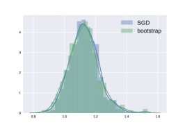
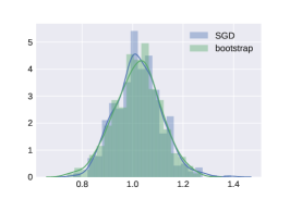
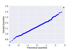
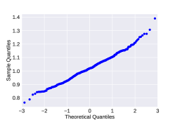
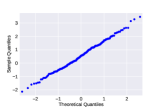
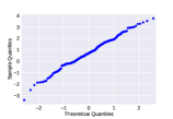
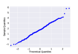
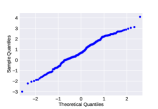
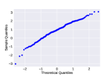
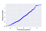
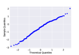
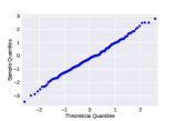
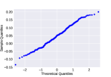
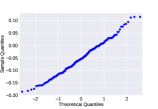
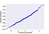
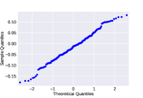
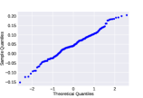
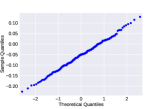
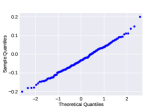
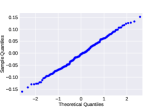
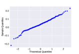
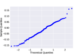
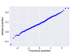
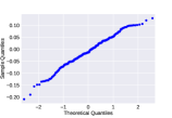
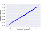
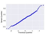
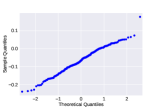
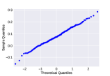
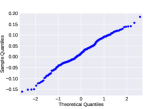
In Figure 2, we compare our SGD inference procedure with Bootstrap and normal approximation with inverse Fisher information in univariate models. We observe that our method and Bootstrap have similar statistical properties. Figure 5 in the appendix shows Q-Q plots of samples from our SGD inference procedure.
Normal distribution mean estimation: Figure 2a compares 500 samples from SGD inference procedure and Bootstrap versus the distribution , using i.i.d. samples from . We used mini batch SGD described in Sec. A. For the parameters, we used , , , , and mini batch size of 2. Our SGD inference procedure gives (0.916 , 0.806), Bootstrap gives (0.926 , 0.841), and normal approximation gives (0.922 , 0.851).
Exponential distribution parameter estimation: Figure 2b compares 500 samples from inference procedure and Bootstrap, using samples from an exponential distribution with PDF where . We used SGD for MLE with mini batch sampled with replacement. For the parameters, we used , , , , and mini batch size of 5. Our SGD inference procedure gives (0.922, 0.364), Bootstrap gives (0.942 , 0.392), and normal approximation gives (0.922, 0.393).
Poisson distribution parameter estimation: Figure 2c compares 500 samples from inference procedure and Bootstrap, using samples from a Poisson distribution with PDF where . We used SGD for MLE with mini batch sampled with replacement. For the parameters, we used , , , , and mini batch size of 5. Our SGD inference procedure gives (0.942 , 0.364), Bootstrap gives (0.946 , 0.386), and normal approximation gives (0.960 , 0.393).
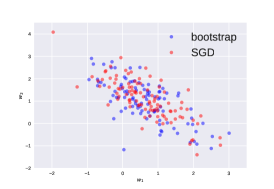
5.1.2 Multivariate models
In these experiments, we set , used mini-batch size of , and used 200 SGD samples. In all cases, we compared with Bootstrap using 200 replicates. We computed the coverage probabilities using 500 simulations. Also, we denote . Additional simulations comparing covariance matrix computed with different methods are given in Sec. D.1.1.
Linear regression: Experiment 1: Results for the case where , , , and with samples is given in Table 1a. Bootstrap gives (0.941, 4.14), and confidence intervals computed using the error covariance and normal approximation gives (0.928, 3.87). Experiment 2: Results for the case where , , , , and with samples is given in Table 1b. Bootstrap gives (0.938, 4.47), and confidence intervals computed using the error covariance and normal approximation gives (0.925, 4.18).
Logistic regression: Here we show results for logistic regression trained using vanilla SGD with mini batch sampled with replacement. Results for modified SGD (Sec. 3.3) are given in Sec. D.1.1. Experiment 1: Results for the case where , with samples is given in Table 2a. Bootstrap gives (0.932, 0.245), and confidence intervals computed using inverse Fisher matrix as the error covariance and normal approximation gives (0.954, 0.256). Experiment 2: Results for the case where , , with samples is given in Table 2b. Bootstrap gives (0.932, 0.253), and confidence intervals computed using inverse Fisher matrix as the error covariance and normal approximation gives (0.957, 0.264).
5.2 Real data
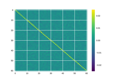
Here, we compare covariance matrices computed using our SGD inference procedure, bootstrap, and inverse Fisher information matrix on the LIBSVM Splice data set, and we observe that they have similar statistical properties.
5.2.1 Splice data set
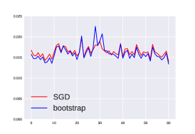
The Splice data set 333https://www.csie.ntu.edu.tw/~cjlin/libsvmtools/datasets/binary.html contains 60 distinct features with 1000 data samples. This is a classification problem between two classes of splice junctions in a DNA sequence. We use a logistic regression model trained using vanilla SGD.
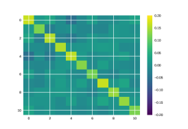
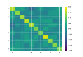
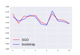
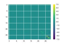
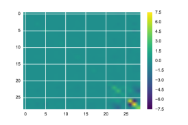
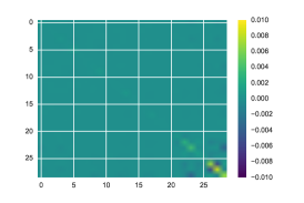
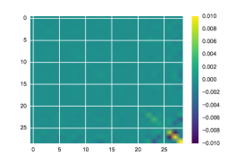
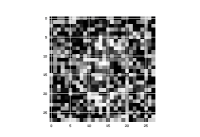
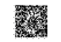
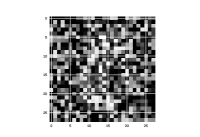
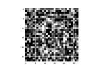
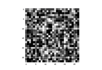
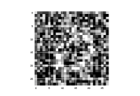
In Figure 3, we compare the covariance matrix computed using our SGD inference procedure and bootstrap samples. We used 10000 samples from both bootstrap and our SGD inference procedure with , , , and mini batch size of .


CI (-64.2, -27.9)
CI (-10.9, 30.5)
5.2.2 MNIST
Here, we train a binary logistic regression classifier to classify 0/1 using a noisy MNIST data set, and demonstrate that adversarial examples produced by gradient attack [GSS15] (perturbing an image in the direction of loss function’s gradient with respect to data) can be detected using prediction intervals. We flatten each image into a 784 dimensional vector, and train a linear classifier using pixel values as features. To add noise to each image, where each original pixel is either 0 or 1, we randomly changed 70% pixels to random numbers uniformly on . Next we train the classifier on the noisy MNIST data set, and generate adversarial examples using this noisy MNIST data set. Figure 4 shows each image’s logit value () and its 95% confidence interval (CI) computed using quantiles from our SGD inference procedure.
5.3 Discussion
In our experiments, we observed that using a larger step size produces accurate results with significantly accelerated convergence time. This might imply that the term in Theorem 1’s bound is an artifact of our analysis. Indeed, although Theorem 1 only applies to SGD with fixed step size, where and imply that the step size should be smaller when the number of consecutive iterates used for the average is larger, our experiments suggest that we can use a (data dependent) constant step size and only require .
In the experiments, our SGD inference procedure uses operations to produce a sample, and Newton method uses operations to produce a sample. The experiments therefore suggest that our SGD inference procedure produces results similar to Bootstrap while using far fewer operations.
6 Acknowledgments
This work was partially supported by NSF Grants 1609279, 1704778 and 1764037, and also by the USDoT through the Data-Supported Transportation Operations and Planning (D-STOP) Tier 1 University Transportation Center. A.K. is supported by the IBM Goldstine fellowship. We thank Xi Chen, Philipp Krähenbühl, Matthijs Snel, and Tom Spangenberg for insightful discussions.
References
- [Bac10] Francis Bach. Self-concordant analysis for logistic regression. Electronic Journal of Statistics, 4:384–414, 2010.
- [Bac14] Francis Bach. Adaptivity of averaged stochastic gradient descent to local strong convexity for logistic regression. Journal of Machine Learning Research, 15(1):595–627, 2014.
- [BEL15] Sebastien Bubeck, Ronen Eldan, and Joseph Lehec. Finite-time analysis of projected langevin monte carlo. In Advances in Neural Information Processing Systems, pages 1243–1251, 2015.
- [BPM90] Albert Benveniste, Pierre Priouret, and Michel Métivier. Adaptive Algorithms and Stochastic Approximations. Springer-Verlag New York, Inc., New York, NY, USA, 1990.
- [BSW14] Pierre Baldi, Peter Sadowski, and Daniel Whiteson. Searching for exotic particles in high-energy physics with deep learning. Nature Communications, 5, 2014.
- [Bub15] Sébastien Bubeck. Convex optimization: Algorithms and complexity. Found. Trends Mach. Learn., 8(3-4):231–357, November 2015.
- [CLTZ16] Xi Chen, Jason Lee, Xin Tong, and Yichen Zhang. Statistical inference for model parameters in stochastic gradient descent. arXiv preprint arXiv:1610.08637, 2016.
- [Efr82] Bradley Efron. The jackknife, the bootstrap and other resampling plans. SIAM, 1982.
- [ET94] Bradley Efron and Robert Tibshirani. An introduction to the bootstrap. CRC press, 1994.
- [GSS15] Ian Goodfellow, Jonathon Shlens, and Christian Szegedy. Explaining and harnessing adversarial examples. In International Conference on Learning Representations, 2015.
- [JZ13] Rie Johnson and Tong Zhang. Accelerating stochastic gradient descent using predictive variance reduction. In Advances in Neural Information Processing Systems, pages 315–323, 2013.
- [KH81] Harold Kushner and Hai Huang. Asymptotic properties of stochastic approximations with constant coefficients. SIAM Journal on Control and Optimization, 19(1):87–105, 1981.
- [KY03] H. Kushner and G.G. Yin. Stochastic Approximation and Recursive Algorithms and Applications. Stochastic Modelling and Applied Probability. Springer New York, 2003.
- [LPW12] Lennart Ljung, Georg Ch Pflug, and Harro Walk. Stochastic approximation and optimization of random systems, volume 17. Birkhäuser, 2012.
- [MHB16] Stephan Mandt, Matthew Hoffman, and David Blei. A Variational Analysis of Stochastic Gradient Algorithms. In Proceedings of The 33rd International Conference on Machine Learning, pages 354–363, 2016.
- [MHB17] Stephan Mandt, Matthew D Hoffman, and David M Blei. Stochastic Gradient Descent as Approximate Bayesian Inference. arXiv preprint arXiv:1704.04289, 2017.
- [OM99] David Opitz and Richard Maclin. Popular ensemble methods: An empirical study. Journal of Artificial Intelligence Research, 11:169–198, 1999.
- [Pfl86] Georg Pflug. Stochastic minimization with constant step-size: asymptotic laws. SIAM Journal on Control and Optimization, 24(4):655–666, 1986.
- [PJ92] Boris Polyak and Anatoli Juditsky. Acceleration of stochastic approximation by averaging. SIAM Journal on Control and Optimization, 30(4):838–855, 1992.
- [PRW12] D.N. Politis, J.P. Romano, and M. Wolf. Subsampling. Springer Series in Statistics. Springer New York, 2012.
- [RM51] Herbert Robbins and Sutton Monro. A stochastic approximation method. The Annals of Mathematical Statistics, pages 400–407, 1951.
- [ST12] Jun Shao and Dongsheng Tu. The jackknife and bootstrap. Springer Science & Business Media, 2012.
- [TA14] Panos Toulis and Edoardo M Airoldi. Asymptotic and finite-sample properties of estimators based on stochastic gradients. arXiv preprint arXiv:1408.2923, 2014.
- [vdV00] A.W. van der Vaart. Asymptotic Statistics. Cambridge Series in Statistical and Probabilistic Mathematics. Cambridge University Press, 2000.
- [Was13] Larry Wasserman. All of statistics: a concise course in statistical inference. Springer Science & Business Media, 2013.
- [WT11] Max Welling and Yee Teh. Bayesian learning via stochastic gradient Langevin dynamics. In Proceedings of the 28th International Conference on Machine Learning, pages 681–688, 2011.
Appendix A Exact analysis of mean estimation
In this section, we give an exact analysis of our method in the least squares, mean estimation problem. For i.i.d. samples , the mean is estimated by solving the following optimization problem
In the case of mini-batch SGD, we sample indexes uniformly randomly with replacement from ; denote that index set as . For convenience, we write , Then, in the mini batch SGD step, the update step is
| (12) |
which is the same as the exponential moving average. And we have
| (13) |
Assume that , then from Chebyshev’s inequality almost surely when . By the central limit theorem, converges weakly to with . From (12), we have uniformly for all , where the constant is data dependent. Thus, for our SGD inference procedure, we have . Our SGD inference procedure does not generate samples that are independent conditioned on the data, whereas replicates are independent conditioned on the data in bootstrap, but this suggests that our SGD inference procedure can produce “almost independent” samples if we discard sufficient number of SGD iterates in each segment.
When estimating a mean using our SGD inference procedure where each mini batch is elements sampled with replacement, we set in (6).
Appendix B Linear Regression
In linear regression, the empirical risk function satisfies:
where denotes the observations of the linear model and are the regressors. To find an estimate to , one can use SGD with stochastic gradient give by:
where are indices uniformly sampled from with replacement.
Next, we state a special case of Theorem 1. Because the Taylor remainder , linear regression has a stronger result than general -estimation problems.
Corollary 2.
Assume that , we have
where and .
We assume that is bounded, and quantities other than and are data dependent constants.
As with our main theorem, in the appendix we provide explicit data-dependent expressions for the constants in the result. Because in linear regression the estimate’s covariance is , we set the scaling factor in (6) for statistical inference.
Appendix C Proofs
C.1 Proof of Theorem 1
We first assume that . For ease of notation, we denote
| (14) |
and, without loss of generality, we assume that . The stochastic gradient descent recursion satisfies:
where . Note that is a martingale difference sequence. We use
| (15) |
to denote the gradient component at index , and the Hessian component at index , at optimum , respectively. Note that and .
For each , its Taylor expansion around is
| (16) |
where is the remainder term. For convenience, we write .
For the proof, we require the following lemmata. The following lemma states that as and .
Lemma 1.
For data dependent, positive constants according to assumptions and in Theorem 1, and given assumption , we have
| (17) |
under the assumption .
Proof.
As already stated, we assume without loss of generality that . This further implies that: , and
Given the above and assuming expectation w.r.t. the selection of a sample from , we have:
| (18) |
where is due to assumptions and of Theorem 1. Taking expectations for every step over the whole history, we obtain the recursion:
∎
The following lemma states that as and .
Lemma 2.
For data dependent, positive constants according to assumptions , , in Theorem 1, we have:
| (19) |
Proof.
Given , we have the following sets of (in)equalities:
| (20) |
where is due to and , is due to assumptions and in Theorem 1, is due to assumptions and in Theorem 1, and is due to . Similar to the proof of the previous lemma, applying the above rule recursively and w.r.t. the whole history of estimates, we obtain:
which is the target inequality, after simple transformations. ∎
We know that:
Using the Taylor expansion formula around the point and using the assumption that , we have:
Taking further the gradient w.r.t. in the above expression, we have:
Using the identity , our SGD recursion can be re-written as:
| (21) |
For and since: , we get:
| (22) |
where holds due to the assumption that the eigenvalues of satisfy , and thus, the geometric series of matrices: , is utilized above. In our case, .
For the latter term in (22), using a variant of Abel’s sum formula, we have:
| (23) | ||||
| (24) |
where follows from the fact , based on the expression (21).
The above combined lead to:
| (25) |
For the main result of the theorem, we are interested in the following quantity:
Using the notation, we have . Thus, we need to bound:
| (26) |
where is due to the successive use of the AM-GM rule:
| (27) |
for two -dimensional random vectors and . Indeed, for any fixed unit vector we have . We used the fact because is convex. Here also, the hides any constants appearing from applying successively the above rule.
Therefore, to proceed bounding the quantity of interest, we need to bound the terms . In the statement of the theorem we have —however similar bounds will hold if ; thus, for each of the above terms we have the following.
| (28) |
| (29) |
where is due to Assumption , is due to Lemma 1, and we used in several places the fact that .
| (30) |
where is due to Assumption and due to , is due to Assumption on bounded remainder, is due to the inequality , is due to , is due to being an small constant compared to and thus .
| (31) |
where is due to for , is due to Assumption , is due to Assumptions and , is due to Lemma 1.
Finaly, for the term , we have
| (32) |
and thus:
For each term , we have
| (33) |
where is due to Assumption , is due to Cauchy-Schwartz inequality and Assumption , is due to Assumption , is due to Lemmas 1-2.
Then, we have:
| (34) |
where is due to Assumption, and is after removing constants and observing that the dominant term in the second part is . Combining all the above in (26), we obtain:
C.2 Proof of Corollary 2
Proof of Corollary 2.
Here we use the same notations as the proof of Theorem 1. Because linear regression satisfies , we do not have to consider the Taylor remainder term in our analysis. And we do not need 4-th order bound for SGD. Due to the fact that the quadratic function is strongly convex, we have .
By sampling with replacement, we have
| (35) |
We also have
| (36) |
where and .
C.3 Proof of Corollary 1
Proof of Corollary 1.
Here we use the same notations as the proof of Theorem 1. Because , is convex. The following lemma shows that is Lipschitz.
Lemma 3.
| (38) |
for some data dependent constant .
Proof.
First, because
| (39) |
we have
| (40) |
Also, we have
| (41) |
which implies
| (42) |
Further:
| (43) |
where step (i) follows from . Thus, we have
| (44) |
and we can conclude that for some data dependent constant . ∎
Next, we show that has a bounded Taylor remainder.
Lemma 4.
| (45) |
for some data dependent constant .
Proof.
Because , we know that when where the constants are data dependent. Because is infinitely differentiable, by the Taylor expansion we know that when where the constants are data dependent. Combining the above, we can conclude for some data dependent constant .
∎
In the following lemma, we will show that for some data dependent constant .
Lemma 5.
| (46) |
for some data dependent constant .
Proof.
We know that
| (47) |
First, notice that locally (when ) we have
| (48) |
because of the optimality condition. This lower bounds when . Next we will lower bound it when .
Consider the function for , we have
| (49) |
where . Because is convex, is an increasing function in , thus we have when . And we can deduce when .
Similarly, because is convex, is an increasing function in . Its derivative when . So we have when .
Thus, we have
| (50) |
when .
And we can conclude that for some data dependent constant . ∎
Next, we will prove properties about .
| (51) |
| (52) |
where follows from and follows from .
Thus, we have
| (53) |
for some data dependent constants and .
For the fourth-moment quantities, we have:
| (54) |
| (55) |
‘where follows from and (ii) follows from .
Combining the above, we get:
| (56) |
for some data dependent constants and .
Finally, we need a bound for the quantity . We observe:
| (57) |
Because
| (58) | ||||
| (59) | ||||
| (60) |
we may conclude that
| (61) |
for some data dependent constants , , , and .
Appendix D Experiments
Here we present additional experiments on our SGD inference procedure.
D.1 Synthetic data

D.1.1 Multivariate models
Here we show Q-Q plots per coordinate for samples from our SGD inference procedure.
Q-Q plots per coordinate for samples in linear regression experiment 1 is shown in Figure 6. Q-Q plots per coordinate for samples in linear regression experiment 2 is shown in Figure 7.
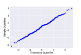
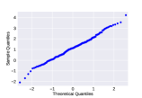
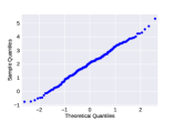
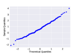
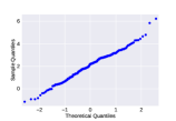
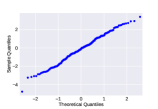

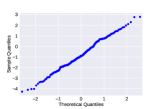
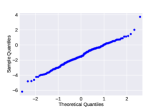
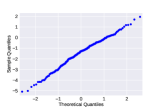
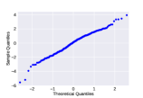
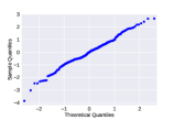
Q-Q plots per coordinate for samples in logistic regression experiment 1 is shown in Figure 8. Q-Q plots per coordinate for samples in logistic regression experiment 2 is shown in Figure 9.


Additional experiments
2-Dimensional Linear Regression. Consider:
Each sample consists of and . We use linear regression to estimate in . In this case, the minimizer of the population least square risk is .
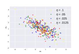
For 300 i.i.d. samples, we plotted 100 samples from SGD inference in Figure 10. We compare our SGD inference procedure against bootstrap in Figure 10a. Figure 10b and Figure 10c show samples from our SGD inference procedure with different parameters.

10-Dimensional Linear Regression.
Here we consider the following model
where , with , and , and use samples. We estimate the parameter using
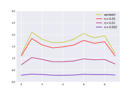
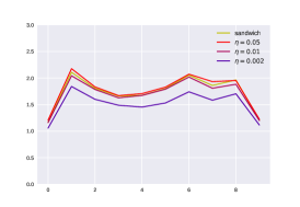
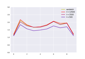
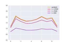
Figure 11 shows the diagonal terms of of the covariance matrix computed using the sandwich estimator and our SGD inference procedure with different parameters. 100000 samples from our SGD inference procedure are used to reduce the effect of randomness.


2-Dimensional Logistic Regression.
Here we consider the following model
| (63) |
We use logistic regression to estimate in the classifier where the minimizer of the population logistic risk is .
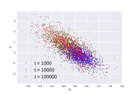
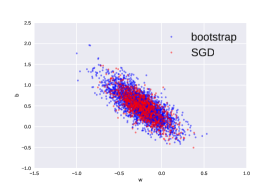
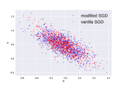
For 100 i.i.d. samples, we plot 1000 samples from SGD in Figure 12. In our simulations, we notice that our modified SGD for logistic regression behaves similar to vanilla logistic regression. T his suggests that an assumption weaker than (assumption () in Theorem 1) is sufficient for SGD analysis. Figure 12b and Figure 12d suggest that the term in Corollary 1 is an artifact of our analysis, and can be improved.


11-Dimensional Logistic Regression.
Here we consider the following model
where and when for some , and . We estimate a classifier using
| (64) |
Figure 13 shows results for with samples. We use , , , and mini batch of size 4 in vanilla SGD. Bootstrap and our SGD inference procedure each generated 2000 samples. In bootstrap, we used Newton method to perform optimization over each replicate, and 6-7 iterations were used. In figure 14, we follow the same procedure for with samples. Here, we use , , ; the rest of the setting is the same.


D.2 Real data
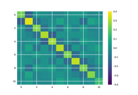
Here, we compare covariance matrix computed using our SGD inference procedure, bootstrap, and inverse Fisher information matrix on the Higgs data set [BSW14] and the LIBSVM Splice data set, and we observe that they have similar statistical properties.
D.2.1 Higgs data set
The Higgs data set 444https://archive.ics.uci.edu/ml/datasets/HIGGS [BSW14] contains 28 distinct features with 11,000,000 data samples. This is a classification problem between two types of physical processes: one produces Higgs bosons and the other is a background process that does not. We use a logistic regression model, trained using vanilla SGD, instead of the modified SGD described in Section 3.3.
To understand different settings of sample size, we subsampled the data set with different sample size levels: and . We investigate the empirical performance of SGD inference on this subsampled data set. In all experiments below, the batch size of the mini batch SGD is 10.
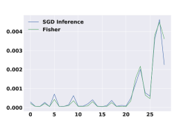
In the case , the asymptotic normality for the MLE is not a good enough approximation. Hence, in this small-sample inference, we compare the SGD inference covariance matrix with the one obtained by inverse Fisher information matrix and bootstrap in Figure 15.
For our SGD inference procedure, we use samples to average, and discard samples. We use averages from 20 segments (as in Figure 1). For bootstrap, we use 2000 replicates, which is much larger than the sample size .
Figure 15 shows that the covariance matrix obtained by SGD inference is comparable to the estimation given by bootstrap and inverse Fisher information.

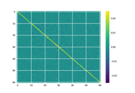
In the case , we use samples to average, and discard samples. We use averages from 20 segments (as in Figure 1). For this large data set, we present the estimated covariance of SGD inference procedure and inverse Fisher information (the asymptotic covariance) in Figure 16 because bootstrap is computationally prohibitive. Similar to the small sample result in Figure 15, the covariance of our SGD inference procedure is comparable to the inverse Fisher information.
In Figure 17, we compare the covariance matrix computed using our SGD inference procedure and inverse Fisher information with samples . We used 25 samples from our SGD inference procedure with , , , and mini batch size of .


D.2.2 Splice data set
The Splice data set 555https://www.csie.ntu.edu.tw/~cjlin/libsvmtools/datasets/binary.html contains 60 distinct features with 1000 data samples. This is a classification problem between two classes of splice junctions in a DNA sequence. Similar to the Higgs data set, we use a logistic regression model, trained using vanilla SGD.
In Figure 18, we compare the covariance matrix computed using our SGD inference procedure and bootstrap samples. We used 10000 samples from both bootstrap and our SGD inference procedure with , , , and mini batch size of .

D.2.3 MNIST
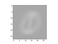
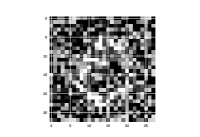
Here, we train a binary logistic regression classifier to classify 0/1 using perturbed MNIST data set, and demonstrate that certain adversarial examples (e.g. [GSS15]) can be detected using prediction confidence intervals. For each image, where each original pixel is either 0 or 1, we randomly changed 70% pixels to random numbers uniformly on . Figure 19 shows each image’s logit value () and its 95% confidence interval computed using our SGD inference procedure. The adversarial perturbation used here is shown in Figure 20 (scaled for display).
CI (-106.4, -30.0)
CI (-6.5, 26.2)
CI (-101.6, -5.5)
CI (-4.9, 11.6)
CI (-75.4, 5.1)
CI (-3.4, 17.9)
CI (-110.7, -32.2)

CI (-8.0, 25.7)