Recurrent Scene Parsing with Perspective Understanding in the Loop

Abstract

Objects may appear at arbitrary scales in perspective images of a scene, posing a challenge for recognition systems that process images at a fixed resolution. We propose a depth-aware gating module that adaptively selects the pooling field size in a convolutional network architecture according to the object scale (inversely proportional to the depth) so that small details are preserved for distant objects while larger receptive fields are used for those nearby. The depth gating signal is provided by stereo disparity or estimated directly from monocular input. We integrate this depth-aware gating into a recurrent convolutional neural network to perform semantic segmentation. Our recurrent module iteratively refines the segmentation results, leveraging the depth and semantic predictions from the previous iterations.

Through extensive experiments on four popular large-scale RGB-D datasets, we demonstrate this approach achieves competitive semantic segmentation performance with a model which is substantially more compact. We carry out extensive analysis of this architecture including variants that operate on monocular RGB but use depth as side-information during training, unsupervised gating as a generic attentional mechanism, and multi-resolution gating. We find that gated pooling for joint semantic segmentation and depth yields state-of-the-art results for quantitative monocular depth estimation.

1 Introduction

Figure 1: Upper: depth-aware gating spatially modulates the selected pooling scale using a depth map predicted from monocular input. In the paper, we also evaluate related architectures where scene depth is provided directly at test time as a gating signal, and where spatially adaptive attentional gating is learned without any depth supervision. Lower: example ground-truth compared to predictions with and without the depth gating module. Rectangles overlayed on the image indicate pooling field sizes which are adapted based on the local depth estimate. We quantize the depth map into five discrete scales in our experiments. Using depth-gated pooling yields more accurate segment label predictions by avoiding pooling across small multiple distant objects while simultaneously allowing using sufficiently large pooling fields for nearby objects.

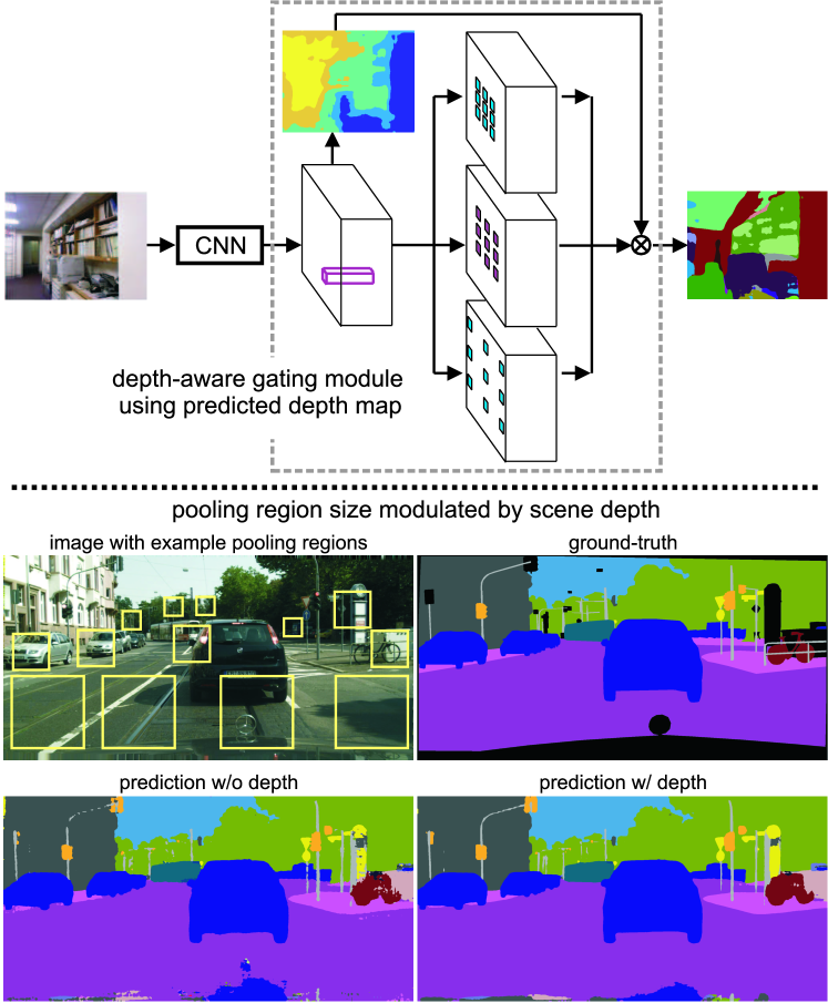
An intrinsic challenge of parsing rich scenes is understanding object layout relative to the camera. Roughly speaking, the scales of the objects in the image frame are inversely proportional to the distance to the camera. Humans easily recognize objects even when they range over many octaves of spatial resolution, e.g., the cars near the camera in urban scene can appear a dozen times larger than those at distance as shown by the lower panel in Figure 1. However, the huge range and arbitrary scale at which objects appear pose difficulties for machine image understanding. Although individual local features (e.g., in a deep neural network) can exhibit some degree of scale-invariance, it is not obvious this invariance covers the range scale variation that exists in images.

In this paper, we investigate how cues to perspective geometry conveyed by image content (estimated from stereo disparity, or measured directly via specialized sensors) might be exploited to improve recognition and scene understanding. We focus specifically on the task of semantic segmentation which seeks to produce per-pixel category labels.

One straightforward approach is to stack the depth map with RGB image as a four-channel input tensor which can then be processed using standard architectures. In practice, this RGB-D input has not proven successful and sometimes even results in worse performance [15, 32]. We conjecture including depth as a per-pixel input doesn’t adequately address scale-invariance in learning; such models lack an explicit mechanism to generalize to depths not observed during training and hence still require training examples with object instances at many different scales to learn a multiscale appearance model.

Instead, our method takes inspiration from the work of [23], who propose using depth estimates to rescale local image patches to a pre-defined canonical depth prior to analysis. For patches contained within a fronto-parallel surface, this can provide true depth-invariance over a range of scales (limited by sensor resolution for small objects) while effectively augmenting the training data available for the canonical depth. Rather than rescaling the input image, we propose a depth gating module that adaptively selects pooling field sizes over higher-level feature activation layers in a convolutional neural network (CNN). Adaptive pooling works with a more abstract notion of scale than standard multiscale image pyramids which operate on input pixels. This gating mechanism allows spatially varying processing over the visual field which can capture context for semantic segmentation that is not too large or small, but “just right”, maintaining details for objects at distance while simultaneously using much larger receptive fields for objects near the camera. This gating architecture is trained with a loss that encourages selection of target pooling scales derived from “ground-truth” depth but at test time makes accurate inferences about scene depth using only monocular cues.

Inspired by studies of human visual processing (e.g., [8]) that suggest dynamic allocation of computation depending on the task and image content (background clutter, occlusion, object scale), we propose embedding gated pooling inside a recurrent refinement module that takes initial estimates of high-level scene semantics as a top-down signal to reprocess feed-forward representations and refine the final scene segmentation (similar to the recurrent module proposed in [4] for human pose). This provides a simple implementation of “Biased Competition Theory” [3] which allows top-down feedback to suppress irrelevant stimuli or incorrect interpretations, an effect we observe qualitatively in our recurrent model near object boundaries and in cluttered regions with many small objects.

We train this recurrent adaptive pooling CNN architecture end-to-end and evaluate its performance on several scene parsing datasets. The monocular depth estimates produced by our gating channel yield state-of-the-art performance on the NYU-depth-v2 benchmark [35]. We also find that using this gating signal to modulate pooling inside the recurrent refinement architecture results in improved semantic segmentation performance over fixed multiresolution pooling. We also compare to gating models trained without depth supervision where the gating signal acts as a generic attentional signal that modulates spatially adaptive pooling. While this works well, we find that depth supervision results in best performance. The resulting system matches state-of-the-art segmentation performance on four large-scale datasets using a model which, thanks to recurrent computation, is substantially more compact than many existing approaches.

2 Related work

Starting from the “fully convolutional” architecture of  [31], there has been a flurry of recent work exploring CNN architectures for semantic segmentation and other pixel-labeling tasks [20]. The seminal DeepLab [6] model modifies the very deep residual neural network [16] for semantic segmentation using dilated or atrous convolution operators to maintain spatial resolution in high-level feature maps. To leverage features conveying finer granularity lower in the CNN hierarchy, it has proven useful to combine features across multiple layers (see e.g., FCN [31], LRR [13] and RefineNet [27]). To simultaneously cover larger fields-of-view and incorporate more contextual information, [38] concatenates features pooled over different scales.

Starting from the work of [17, 34], estimating depth from (monocular) scene semantics has been examined in a variety of indoor and outdoor settings (see e.g., [25]). Accurate monocular depth estimation using a multiscale deep CNN architecture was demonstrated by [11] using a geometrically inspired regression loss. Follow-on work [10] showed that depth, surface orientation and semantic labeling predictions can benefit each other in a multi-task setting using a shared network model for feature extraction.

The role of perspective geometry and geometric context in object detection was emphasized by a line of work starting with [18] and others (e.g., [2]) and has played an increasingly important role, particularly for scene understanding in urban environments [12]. We were inspired by [23], who showed reliable depth recovery from image patches (i.e., without vanishing point estimation) and that the resulting depths could be used to estimate object scale and improve segmentation in turn. Chen et al. [7] used an attention gating mechanism to combine predictions from CNN branches run on rescaled images (multi-resolution), a natural but computationally expensive approach that we compare experimentally to our proposal (multi-pool).

Finally, there have been a number of proposals to carry out high-level recognition tasks such as human pose estimation [26, 4] and semantic segmentation [33] using recurrent or iterative processing. As pixel-wise labelling tasks are essentially a structured prediction problem, there has also been a related line of work that aims to embed unrolled conditional random fields or mean shift into differentiable CNN architectures to allow for more tractable learning and inference (e.g., [39, 20]).

Figure 2: The input to our recurrent module is the concatenation (denoted by $\oslash$) of the feature map from an intermediate layer of the feed-forward pathway with the prior recurrent prediction. Our recurrent module utilizes depth-aware gating which carries out both depth regression and quantized prediction. Updated depth predictions at each iteration gate pooling fields used for semantic segmentation. This recurrent update of depth estimation increases the flexibility and representation power of our system yielding improved segmentation. We illustrate the prediction prior to, and after two recurrent iterations for a particular image and visualize the difference in predictions between consecutive iterations which yield small but notable gains as measured by average intersection-over-union (IoU) benchmark performance.

3 Depth-aware Gating Module

Our depth-aware gating module utilizes estimated depth at each image location as a proxy for object scale in order to select the appropriate spatial extent over which to pool features. Informally speaking, for a given object category (e.g., cars) the size of an object in the image is inversely proportional to the distance from the camera. Thus, if a region of an image has a larger depth values, the windows over which features are pooled (pooling field size) should be smaller in order to avoid pooling responses over many small objects and capture details needed to precisely segment small objects. For regions with small depth values, the same object will appear much larger and the pooling field size should be scaled up in a covariant manner to capture sufficient contextual appearance information in the vicinity of the object.

This depth-aware gating can readily utilize depth maps derived from stereo disparity or specialized time-of-flight sensors. Such depth maps typically contain missing data and measurement noise due to oblique view angle, reflective surface and occlusion boundary. While these estimates can be improved using more extensive off-line processing (e.g., [36]), in our experiments we use these “raw” measurements. When depth measurements are not available, the depth-aware gating can instead exploit depth estimated directly from monocular cues. The upper panel of Figure 1 illustrates the architecture of our depth-aware gating module using monocular depth predictions derived from the same front-end feature extractor.

Regardless of the source of the depth map, we quantize the depth into a discrete set of predicted scales (5 in our experiments). The scale prediction at each image location is then used to multiplicatively gate between a set of feature maps computed with corresponding pooling regions and summed to produce the final feature representation for classification [21, 19]. In the depth gating module, we use atrous convolution with different dilation rates to produce the desired pooling field size on each branch.

When training a monocular depth prediction branch, we quantize the ground-truth depth and treat it as a five-way classification using a softmax loss. For the purpose of quantitatively evaluating the accuracy of such monocular depth prediction, we also train a depth regressor over the input feature of the module using a simple Euclidean loss for the depth map ${\bf D}$ in log-space:

$$\small\begin{split}\ell_{depthReg}({\bf D},{\bf D}^{*})=&\frac{1}{|M|}\sum_{(i,j)\in M}\|\log({\bf D}_{ij})-\log({\bf D}_{ij})^{*}\|_{2}^{2},\end{split}$$

where ${\bf D}^{*}$ is the ground-truth depth. Since our “ground-truth” depth may have missing entries, we only compute the loss over pixels inside a mask $M$ which indicates locations with valid ground-truth depth. For benchmarking we convert the log-depth predictions back to depths using an element-wise exponential. Although more specific depth-oriented losses have been explored [11, 10], we show in experiment that this simplistic Euclidean loss on log-depth achieves state-of-the-art monocular depth estimation when combined with our architecture for semantic segmentation.

In our experiments, we evaluate models based on RGB-D images (where the depth channel is used for gating) and on RGB images using the monocular depth estimation branch. We also evaluated a variant which is trained monocularly (without the depth loss) where the gating can be viewed as a generic attentional mechanism. In general, we find that using predicted (monocular) depth to gate segmentation feature maps yields better performance than models using the ground-truth depth input. This is a surprising, but desirable outcome, as it avoids the need for extra sensor hardware and/or additional computation for refining depth estimates from multiple video frames (e.g.,  [36]).

4 Recurrent Refinement Module

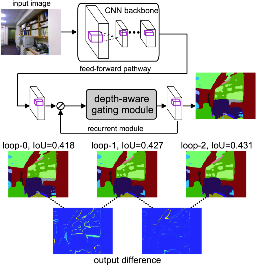
It is natural that scene semantics and depth may be helpful in inferring each other. To achieve this, our recurrent refinement module takes as input feature maps extracted from a feed-forward CNN model along with current segmentation predictions available from previous iterations of the recurrent module. These are concatenated into a single feature map. This allows the recurrent module to provide an anytime segmentation prediction which can be dynamically refined in future iterations. The recurrent refinement module has multiple convolution layers, each of which is followed by a ReLU and batch normalization layers. We also use depth-aware gating in the recurrent module, allowing the refined depth output to serve as a top-down signal for use in refining the segmentation (as shown in experiments below). Figure 2 depicts our final recurrent architecture using the depth-aware gating module inside.

For a semantic segmentation problem with $K$ semantic classes, we use a $K$-way softmax classifier on individual pixels to train our network. Our final multi-task learning objective function utilizes multiple losses weighted by hyperparameters:

$$\begin{split}\ell=&\sum\limits_{l=0}^{L}(\lambda_{s}\ell_{segCls}^{l}+\lambda_{r}\ell_{depthReg}^{l}+\lambda_{c}\ell_{depthCls}^{l}),\\ \end{split}$$ (1)

where $L$ means we unroll the recurrent module into $L$ loops and $l=0$ denotes the prediction from the feed-forward pathway. The three losses $\ell_{segCls}^{l}$, $\ell_{depthReg}^{l}$ and $\ell_{depthCls}^{l}$ correspond to the semantic segmentation, depth regression and quantized depth classification loss at iteration $l$, respectively. We train our system in a stage-wise procedure by varying the hyper-parameters $\lambda_{s}$, $\lambda_{r}$ and $\lambda_{c}$, as detailed in Section 5, culminating in end-to-end training using the full objective. As our primary task is improving semantic segmentation, in the final training stage we optimize only $\ell_{segCls}^{l}$ and drop the depth side-information (setting $\lambda_{r}=0$ and $\lambda_{c}=0$).

5 Implementation

We implement our model with the MatConvNet toolbox [37] and train using SGD on a single Titan X GPU. We use the pre-trained ResNet50 and ResNet101 models [16] as the backbone of our models. To increase the output resolution of ResNet, like [6], we remove the top global $7\times 7$ pooling layer and the last two $2\times 2$ pooling layers. Instead we apply atrous convolution with dilation rate 2 and 4, respectively to maintain a spatial sampling rate which is of $1/8$ resolution to the original image size (rather than $1/32$ resolution if all pooling layers are kept). To obtain a final full resolution segmentation prediction, we simply apply bilinear interpolation on the softmax class scores to upsample the output by a factor of eight.

We train our models in a stage-wise procedure. First, we train a feed-forward baseline model for segmentation. The feed-forward module is similar to DeepLab [6], but we add two additional $3\times 3$-kernel layers (without atrous convolution) on top of the ResNet backbone. Starting from this baseline, we train depth estimation branch and replace the second $3\times 3$-kernel layer with the depth prediction and depth-aware gating module. We train the recurrent refinement module (containing the depth-aware gating), unrolling one layer at a time, and fine-tune the whole system using the objective function of Eq. 1.

We augment the training set using random data transforms. Specifically, we use random scaling by $s\in[0.5,2]$, in-plate rotation by degrees in $[-10^{\circ},10^{\circ}]$, random left-right flip with 0.5 probability, random crop with sizes around $700\times 700$ divisible by 8, and color jittering. Note that when scaling the image by $s$, we also divide the depth values by $s$. All these data transforms can be performed in-place with minimal computational cost.

Throughout training, we set batch size to one where the batch is a single input image (or a crop of a very high-resolution image). Due to this small batch size, we freeze the batch normalization in ResNet backbone during training, using the same constant global moments in both training and testing. We use the “poly” learning rate policy [6] with a base learning rate of $2.5e-4$ scaled as a function of iteration by $(1-\frac{iter}{maxiter})^{0.9}$.

6 Experiments

To show the effectiveness of our approach, we carry out comprehensive experiments on four large-scale RGB-D datasets (introduced below). We start with a quantitative evaluation of our monocular depth predictions, which achieve state-of-the-art performance. We then compare our complete model with the existing methods for semantic segmentation on these datasets, followed by ablation experiments to determine whether our depth-aware gating module improves semantic segmentation, validate the benefit of our recurrent module, and compare among using ground-truth depth, predicted depth, and unsupervised attentional gating. Finally, we show some qualitative results.

6.1 Datasets and Benchmarks

For our primary task of semantic segmentation, we use the standard Intersection-over-Union (IoU) criteria to measure the performance. We also report the per-pixel prediction accuracy for the first three datasets to facilitate comparison to existing approaches.

NYUD-depth-v2 [35] consists of 1,449 RGB-D indoor scene images of the resolution $640\times 480$ which include color and pixel-wise depth obtained by a Kinect sensor. We use the ground-truth segmentation into 40 classes provided in [14] and a standard train/test split into 795 and 654 images respectively.

SUN-RGBD [36] is an extension of NYUD-depth-v2 [35], containing 5,285 training images and 5,050 testing images. It provides pixel labelling masks for 37 classes, and depth maps using different depth cameras. While this dataset provides refined depth maps (exploiting depth from the neighborhood video frames), the ground-truth depth maps still have significant noisy/mislabled depth (examples can be found in our supplemental material).

Cityscapes [9] contains high quality pixel-level annotations of images collected in street scenes from 50 different cities. The training, validation, and test sets contain 2,975, 500, and 1,525 images respectively labeled for 19 semantic classes. The images of Cityscapes are of high resolution ($1024\times 2048$), which makes training challenging due to limited GPU memory. We randomly crop out sub-images of $800\times 800$ resolution for training.

Stanford-2D-3D [1] contains 1,559 panoramas as well as depth and semantic annotations covering six large-scale indoor areas from three different buildings. We use area 3 and 4 as a validation set (489 panoramas) and the remaining four areas for training (1,070 panoramas). The panoramas are very large ($2048\times 4096$) and contain black void regions at top and bottom due to the spherical panoramic topology. For the task of semantic segmentation, we rescale them by $0.5$ and crop out the central two-thirds ($y\in[160,863]$) resulting in final images of size $704\times 2048$-pixels.

Table 1: Depth prediction on NYU-depth-v2 dataset.

Metric $\delta<$	Ladicky [23]	Liu [30]	Eigen [11]	Eigen [10]	Laina [24]	Ours	Ours -blur
$1.25$	0.542	0.614	0.614	0.769	0.811	0.809	0.816
$1.25^{2}$	0.829	0.883	0.888	0.950	0.953	0.945	0.950
$1.25^{3}$	0.940	0.971	0.972	0.988	0.988	0.986	0.989

6.2 Depth Prediction

Figure 3: Examples of monocular depth predictions. First row: the input RGB image; second row: ground-truth; third row: our result. In our visualizations, all depth maps use the same fixed (absolute) colormap to represent metric depth.

In developing our approach, accurate depth prediction was not the primary goal, but rather generating a quantized gating signal to select the pooling field size. However, to validate our depth prediction, we also trained a depth regressor over the segmentation backbone and compared the resulting predictions with previous work. We evaluated our model on NYU-depth-v2 dataset, on which a variety of depth prediction methods have been tested. We report performance using the standard threshold accuracy metrics, i.e., the percentage of predicted pixel depths $d_{i}$ s.t. $\delta=\max(\frac{d_{i}}{d_{i}^{*}},\frac{d_{i}^{*}}{d_{i}})<\tau$, evaluated at multiple thresholds $\tau=\{1.25,1.25^{2},1.25^{3}\}$.

Table 1 provides a quantitative comparison of our predictions with several published methods. We can see our model trained with the Euclidean loss on log-depth is quite competitive and achieves significantly better performance in the $\delta<1.25$ metric. This simplistic loss compares well to, e.g., [10] who develop a scale-invariant loss and use first-order matching term which compares image gradients of the prediction with the ground-truth, and [24] who develop a set of sophisticated upsampling layers over a ResNet50 model.

In Figure 3, we visualize our estimated depth maps on the NYU-depth-v2 dataset. Visually, we can see our predicted depth maps tend to be noticeably less smooth than true depth. Inspired by [10] who advocate modeling smoothness in the local prediction, we also apply Gaussian smoothing on our predicted depth map. This simple post-process is sufficient to outperform the state-of-the-art. We attribute the success of our depth estimator to two factors. First, we use a deeper architecture (ResNet50) than that in [10] which has generally been shown to improve performance on a variety vision tasks as reported in literature. Second, we train our depth prediction branch jointly with features used for semantic segmentation. This is essentially a multi-task problem and the supervision provided by semantic segmentation may understandably help depth prediction, explaining why our blurred predictions are as good or better than a similar ResNet50-based approach which utilized a set of sophisticated upsampling layers [24].

Table 2: Performance of semantic segmentation on different datasets. Results marked by ^† are from our trained model models with the released code, and results marked by ^∗ are evaluated by the dataset server on test set. Note that we train our models based on ResNet50 architecture on indoor datasets NYU-depth-v2 and SUN-RGBD, and ResNet101 on the large perspective datasets Cityscapes and Stanford-2D-3D.

	NYU-depth-v2 [35]			SUN-RGBD [35]			Stanford-2D-3D [1]			Cityscapes [9]
	IoU	pixel acc.		IoU	pixel acc.		IoU	pixel acc.		IoU
baseline	0.406	0.703		0.402	0.776		0.644	0.866		0.738
w/ gt-depth	0.413	0.708		0.422	0.787		0.730	0.897		0.753
w/ pred-depth	0.418	0.711		0.423	0.789		0.742	0.900		0.759
loop1 w/o depth	0.419	0.706		0.432	0.793		0.744	0.901		0.762
loop1 w/ gt-depth	0.425	0.711		0.439	0.798		0.747	0.902		0.769
loop1 w/ pred-depth	0.427	0.712		0.440	0.798		0.753	0.906		0.772
loop2	0.431	0.713		0.443	0.799		0.760	0.908		0.776
loop2 (test-aug)	0.445	0.721		0.451	0.803		0.765	0.910		0.791 / $0.782^{*}$
DeepLab [6]	-	-		-	-		0.698†	0.880†		0.704 / $0.704^{*}$
LRR [13]	-	-		-	-		-	-		0.700 / $0.697^{*}$
Context [28]	0.406	0.700		0.423	0.784		-	-		-       / $0.716^{*}$
PSPNet [38]	-	-		-	-		0.674†	0.876†		-      / $0.784^{*}$
RefineNet-Res50 [27]	0.438	-		-	-		-	-		-       /     -
RefineNet-Res101 [27]	0.447	-		0.457	0.804		-	-		-       / $0.736^{*}$
RefineNet-Res152 [27]	0.465	0.736		0.459	0.806		-	-		-       /     -

6.3 Semantic Segmentation

To validate the proposed depth-aware gating module and the recurrent refinement module, we evaluate several variants over our baseline model. We list the performance details in the first group of rows in Table 2. The results are consistent across models trained independently on the four datasets. Adding depth maps for gating feature pooling brings noticeable boost in segmentation performance, with greatest improvements especially on the large-perspective datasets Cityscapes and Stanford-2D-3D.

Interestingly, we achieve slightly better performance using the predicted depth map rather than the provided ground-truth depth. We attribute this to three explanations. Firstly, the predicted depth is smooth without holes or invalid entries. When using raw depth, say on Cityscapes and Stanford-2D-3D, we assign equal weight on the missing entries so that the gating actually averages the information at different scales. This average pooling might be harmful in some cases such as a very small object at a distance. Secondly, the predicted depth maps show some object-aware patterns (e.g., car region shown in the visualization in Figure 7), which might be helpful for class-specific segmentation. Thirdly, the model is trained end-to-end so co-adaption of the depth prediction and segmentation branches may increase the overall representation power and flexibility of the whole model, benefiting the final predictions.

Table 2 also shows the benefit of the recurrent refinement module as shown by improved performance from baseline to loop1 and loop2. Equipped with depth in the recurrent module, the improvement is more notable. As with the pure feed-forward model, using predicted depth maps in the recurrent module yields slight gains over the ground-truth depth. We observe that performance improves using a depth 2 unrolling (third group of rows in Table 2) but saturates/converges after two iterations.

In comparing with state-of-the-art methods, we follow common practice of augmenting images at test time by running the model on flipped and rescaled variants and average the class scores to produce the final segmentation output (compare loop2 and loop2 (test-aug)). We can see our model performs on par or better than recently published results listed in Table 2.

Note that for NYU-depth-v2 and SUN-RGBD, our backbone architecture is ResNet50, whereas RefineNet reports the results using a much deeper models (ResNet101 and ResNet152) which typically outperform shallower networks in vision tasks. For the Cityscapes, we also submitted our final result for held-out benchmark images which were evaluated by the Cityscapes benchmark server. Our model achieves IoU $0.782$, on par with the best published result, IoU $0.784$, by PSPNet. We did not perform any extensive performance tuning and only utilized the fine-annotation training images for training (without the twenty thousand coarse-annotation images and the validation set). We also didn’t utilize any post-processing (such as the widely used fully-connected CRF [22] which typical yields additional performance increments).

One key advantage of recurrent refinement is that it allows richer computation (and better performance) without additional model parameters. Our ResNet50 model (used on the NYU-depth-v2 dataset) is relatively compact (221MB) compared to RefineNet-Res101 which achieves similar performance but is nearly double the size (426MB). Our model architecture is similar to DeepLab which also adopts pyramid atrous convolution at multiple scales of inputs (but simply averages output feature maps without any depth-guided adaptive pooling). However, the final DeepLab model utilizes an ensemble which yields a much larger model (530MB). PSPNet concatenates the intermediate features into 4,096 dimension before classification while our model operates on small 512-dimension feature maps.

Figure 4: Performance comparisons across gating architectures including tied vs untied parameters across different branches, averaging vs gating branch predictions, using monocular predicted vs ground-truth depth for the gating signal, gating pooling region size (MultiPool) or rescaling input image (MultiScale), and gating without depth supervision during training (attention).

Figure 5: Visualization of the attention maps on random images from Cityscapes and Stanford-2D-3D. The raw disparity/depth maps and the quantized versions are also shown for reference. Though we train the attention branch with randomly initialized weights, we can see that the learned attention maps capture some depth information as well as encoding distance to object boundaries.

Figure 6: Visualization of the output on NYU-depth-v2. We show four randomly selected testing images with ground-truth and predicted disparity (first row), quantized disparity (second row) and segmentation (third row) at each iteration of the recurrent computation.

Figure 7: Visualization of randomly selected validation images from Cityscapes and Stanford-2D-3D with the segmentation output and the predicted quantized disparity at each iteration of the recurrent loop. We depict “ground-truth” continuous and quantized disparity beneath the input image. Our monocular disparity estimate makes predictions for reflective surfaces where stereo fails and recurrent iteration further improves estimates, particularly for featureless areas such as the pavement. Note that Cityscapes shows disparity while Stanford-2D-3D shows depth so the colormaps are reversed.

6.4 Analysis of Gating Architectures Alternatives

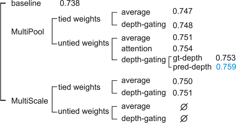
We discuss the important question of whether depth-aware gating is really responsible for improved performance over baseline, or if gains are simply attributable to training a larger, richer architecture. We also contrast our approach to a number of related proposals in the literature. We summarize our experiments exploring these alternatives in Figure 4 (more details can be found in supplementary material).

We use the term MultiPool to denote the family of models (like our proposed model) which process the input image at a single fixed scale, but perform pooling at multiple convolutional dilate rate at high level layers. For a multi-pool architecture, we may choose to learn independent untied weights across the scale-specific branches or use the same tied weights. As an alternative to our gating function, which selects a spatially varying weighted combination of the scale-specific branches, we can simply average the branches (identical at all spatial locations).

We can contrast MultiPool with the MultiScale approach, which combines representations or predictions from multiple branches where each branch is applied to a scaled version of the input image. Many have adopted this strategy as a test time heuristic to boost performance by simply running the same model (tied) on different scaled versions of the input and then averaging the predictions. Others, such as DeepLab [6], train multiple (untied) models and use the average ensemble output.

In practice, we found that both MultiPool and MultiScale architectures outperform baseline and achieve similar performance. While MultiScale processing is conceptually appealing, it has a substantial computational overhead relative to MultiPool processing (where early computation is shared among branches). As a result, it was not feasible to train untied MultiScale models end-to-end on a single GPU memory constraints. As a result, we found that the untied, depth-gated model performed the best (and was adopted in our final approach).

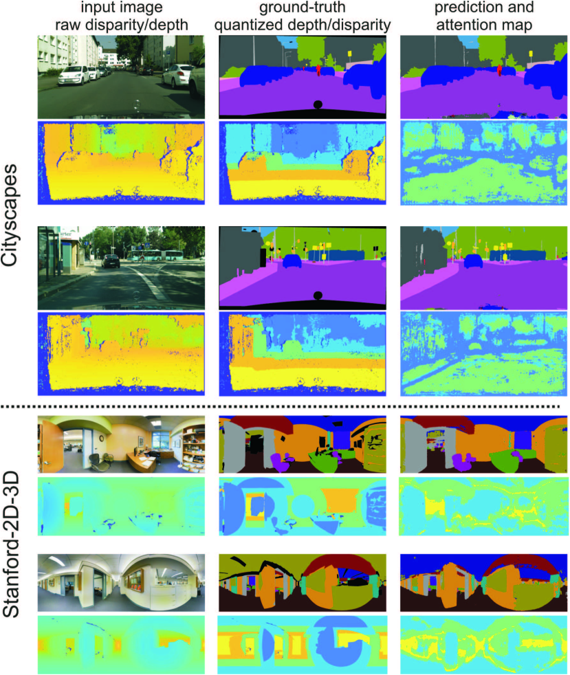
Finally, we explored use of the gated pooling where the gating was trained without the depth loss. We refer to this as an attention model after the work of [7]. The attention model achieves surprisingly good performance, even outperform gating using ground-truth depth. We show the learned attention map in Figure 5, which behaves quite differently from depth gating. Instead, the gating signal appears to encode the distance from object boundaries. We hypothesize this selection mechanism serves to avoid pooling features across different semantic segments while still utilizing large pooling regions within each region. Our fine-tuned model using predicted depth-gating (instead of ground-truth depth) likely benefits from this adaption.

6.5 Qualitative Results

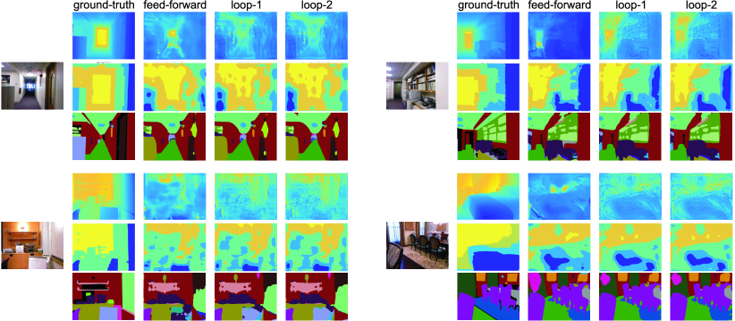
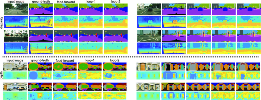
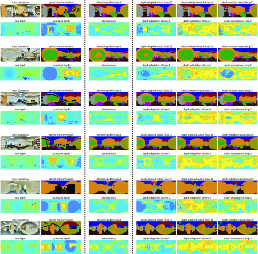
In Figures 6 and 7, we depict several randomly selected examples from the test set of NYU-depth-v2, Cityscapes and Stanford-2D-3D. We visualize both the segmentation results and the depth maps updated across multiple recurrent iterations. Interestingly, the depth maps on Cityscapes and Stanford-2D-3D change more noticeably than those on NYU-depth-v2 dataset. In Cityscapes, regions in the predicted depth map corresponding to objects, such as the car, are grouped together and disparity estimates on texture-less regions such as the street surface improve across iterations, while in Stanford-2D-3D, depth estimate for adaptation suggests that the recurrent module is performing coarse-to-fine segmentation (where later iterations shift towards a smaller pooling regions as semantic confidence increases).

Gains for the NYU-depth-v2 data are less apparent. We conjecture this is because images in NYU-depth-v2 are more varied in overall layout and often have less texture and fewer objects from which the model can infer semantics and subsequently depth. In all datasets, we can see that our model is able to exploit recurrence to correct misclassified regions/pixels “in the loop”, visually demonstrating the effectiveness of the recurrent refinement module.

7 Conclusion and Discussion

In this paper, we have proposed a depth-aware gating module that uses depth estimates to adaptively modify the pooling field size at a high level layer of neural network for better segmentation performance. The adaptive pooling can use large pooling fields to include more contextual information for labeling large nearby objects, while maintaining fine-scale detail for objects further from the camera. While our model can utilize stereo disparity directly, we find that using such data to train a depth predictor which is subsequently used for adaptation at test-time in place of stereo ultimately yields better performance. We also demonstrate the utility of performing recurrent refinement which yields improved prediction accuracy for semantic segmentation without adding additional model parameters.

We envision that the recurrent refinement module can capture object shape priors, contour smoothness and region continuity. However, our current approach converges after a few iterations and performance saturates. This leaves open future work in exploring other training objectives that might push the recurrent computation towards producing more varied outputs. This might be further enriched in the setting of video where the recurrent component could be extended to incorporate memory of previous frames.

Page 0 of the manuscript.

8 Analysis of Depth-aware Gating Module

In this section, we analyze the proposed depth-aware gating module with detailed results in Table 3. We perform the ablation study on the Cityscapes dataset [9]. Specifically, we train the following models in order (except the fourth model which learns attention to gate).

1. “baseline” is our DeepLab-like baseline model by training two convolutional (with $3\times 3$ kernels) layers above the ResNet101 backbone.

2. “tied, avg.” is the model we train based on “baseline” by using the same $3\times 3$ kernel but different dilate rates equal to $\{1,2,4,8,16\}$, respectively. So there are five branches and each of them has the same kernels which are tied to make processing scale-invariant. We average the feature maps for the final output prior to classification.

3. “gt-depth, tied, gating” is the model using the ground-truth depth map to select the branch; the pooling window size is determined according to the ground-truth depth value.

4. “gt-depth, untied, gating” is the model based on “gt-depth, tied, gating” by unleashing the tied kernels in the five branches. These untied kernels improve the flexibility and representation power of the network. Figure 8 (a) depicts this model.

5. “attention, untied, gating” is an independent model to the previous ones that is trained without depth supervision where the gating signal acts as a generic attentional signal that modulates spatially adaptive pooling. Specifically, we train an attention branch to produce the soft weight mask after softmax to gate the features from multiple pooling at different scales. We also adopt untied weights for the scale-specific pooling branches. The architecture is similar to what depicted in Figure 8 (b), but without depth supervision.

6. “pred-depth, untied, gating” is our final model in which we learn a quantized depth predictor to gate the five branches. This model determines the size of pooling window based on its predicted depth map. Figure 8 (b) shows the architecture of this model.

Through Table 3, we can see that increasing the dilate rate with our model “tied, avg.” improves the performance noticeably. This is consistent with the observation in [6], in which the large view-of-field version of DeepLab performs better. The benefit can be explained by the large dilation rate increasing the size of the receptive field, allowing more contextual information to be captured at higher levels of the network. With the gating mechanism, either using ground-truth depth map or the predicted one, the performance is improved further over non-adaptive pooling. The depth-aware gating module helps determine the pooling window size wisely, which is better than averaging all branches equally as in our “tied, avg.” model and DeepLab. Moreover, by unleashing the tied kernels, the “gt-depth untied, gating” improves over “gt-depth, tied, gating” remarkably. We conjecture that this is because the untied kernels provide more flexibility to distinguish features at different scales and allow selection of the appropriate non-invariant features from lower in the network. Interestingly, the attention-gating model performs well and using the predicted depth map achieves the best among all these compared models. We attribute this to three reasons. Firstly, the predicted depth is smooth without holes or invalid entries. When using ground-truth depth on Cityscapes dataset, we assign equal weight on the missing entries so that the gating actually averages the information at different scales. This average pooling might be harmful in some cases such as very small object at distance. This can be taken as complementary evidence that the blindly averaging all branches achieves inferior performance to using the depth-aware gating. Secondly, the predicted depth maps have some object-aware pattern structure, which might be helpful for segmentation. From the visualization shown later in Figure 11, we can observe such patterns, e.g. for cars. Thirdly, the depth prediction branch, as well as the attention branch, generally increases the representation power and flexibility of the whole model; this can be beneficial for segmentation.

Figure 8: (a) Depth-aware gating module using the ground-truth depth map, and (b) depth-aware gating module using the predicted depth map. The grids within the feature map blocks distinguish different pooling field sizes. Here we depict three different pooling window sizes while in our actual experiments we quantize the depth map into five scale bins.

Table 3: Result of different depth-aware gating module deployments on Cityscapes dataset. IoU is short for intersection over union averaged over all classes, and nIoU is the weighted IoU through the pre-defined class weights provided by the benchmark.

	baseline			tied, avg.			gt-depth, tied, gating			gt-depth, untied, gating			attention, untied, gating			pred-depth, untied, gating
	IoU	nIoU		IoU	nIoU		IoU	nIoU		IoU	nIoU		IoU	nIoU
Score Avg.	0.738	0.547		0.747	0.554		0.748	0.556		0.753	0.561		0.754	0.558		0.759	0.571
road	0.980	–		0.981	–		0.981	–		0.982	–		0.982	–		0.982	–
sidewalk	0.849	–		0.847	–		0.849	–		0.982	–		0.853	–		0.857	–
building	0.916	–		0.917	–		0.918	–		0.919	–		0.923	–		0.920	–
wall	0.475	–		0.499	–		0.506	–		0.511	–		0.527	–		0.512	–
fence	0.596	–		0.605	–		0.605	–		0.611	–		0.618	–		0.614	–
pole	0.598	–		0.599	–		0.604	–		0.616	–		0.615	–		0.624	–
traffic light	0.684	–		0.674	–		0.678	–		0.692	–		0.689	–		0.699	–
traffic sign	0.780	–		0.776	–		0.775	–		0.782	–		0.783	–		0.790	–
vegetation	0.918	–		0.917	–		0.918	–		0.920	–		0.920	–		0.922	–
terrain	0.619	–		0.620	–		0.627	–		0.632	–		0.625	–		0.638	–
sky	0.941	–		0.937	–		0.940	–		0.942	–		0.943	–		0.944	–
person	0.803	0.635		0.803	0.631		0.804	0.639		0.808	0.648		0.804	0.641		0.814	0.659
rider	0.594	0.448		0.595	0.462		0.602	0.460		0.612	0.461		0.602	0.443		0.616	0.473
car	0.939	0.859		0.942	0.854		0.942	0.863		0.942	0.867		0.943	0.862		0.944	0.871
truck	0.631	0.398		0.666	0.421		0.679	0.407		0.679	0.417		0.666	0.424		0.674	0.421
bus	0.759	0.595		0.802	0.607		0.787	0.612		0.786	0.609		0.798	0.602		0.799	0.615
train	0.621	0.467		0.683	0.494		0.656	0.489		0.655	0.487		0.684	0.508		0.687	0.507
motorcycle	0.562	0.396		0.587	0.387		0.591	0.398		0.602	0.410		0.583	0.407		0.610	0.425
bicycle	0.755	0.582		0.747	0.387		0.753	0.575		0.761	0.586		0.760	0.575		0.765	0.594

9 Results on the SUN-RGBD dataset

Figure 9: Visualization of images from SUN-RGBD dataset and their ground-truth depth and our predicted depth on the three rows, respectively. We scale all the depth maps into a fixed range of $[0,10^{5}]$. In this sense, the color of the depth maps directly reflect the absolute physical depth. Note that there are unnatural regions in the ground-truth depth maps, which have been refined by the algorithm in [36]. Visually, these refined region do not always make sense and are incorrect depth completions. In contrast, our monocular predictions are quite smooth.

Figure 10: Visualization of the output on SUN-RGBD dataset. We randomly show fourteen images from validation set with their segmentation output from both feed-forward pathway and recurrent loops. In the ground-truth segmentation annotation, we can see that there are many regions (with black color) not annotated.

In Figure 9, we show the depth prediction results of several images randomly picked from the test set of SUN-RGBD dataset. Note that the there are unnatural regions in the ground-truth depth maps, which are the result of refined depth completion by the algorithm in [36]. Visually, these regions do not always make sense and constitute bad depth completions. In contrast, our predicted depth maps are much smoother. We also evaluate our depth prediction on SUN-RGBD dataset, and achieve 0.754, 0.899 and 0.961 by the three threshold metrics respectively. As SUN-RGBD is an extension of NYU-depth-v2 dataset, it has similar data statistics resulting in similar prediction performance.

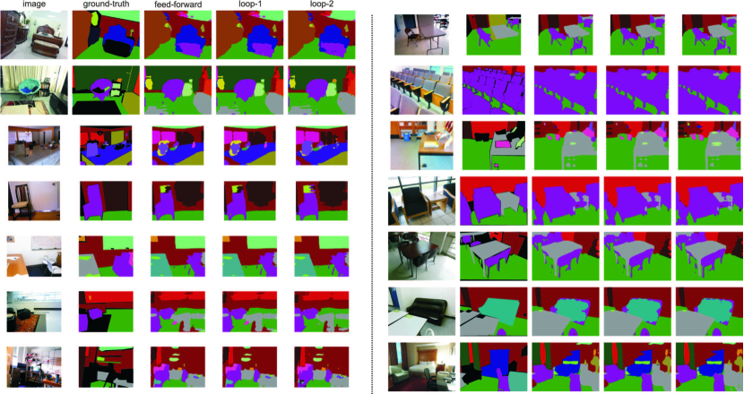
In Figure 10, we randomly show fourteen images and their segmentation results at loops of the recurrent refining module. Visually, we can see that the our recurrent module refines the segmentation result in the loops.

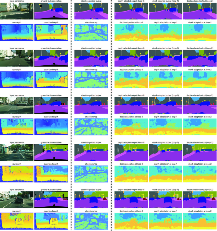
10 Visualization on Large Perspective Images

Figure 11: Visualization of the results on Cityscapes dataset. For five random images from the validation set, we show the input perspective street scene photos, ground-truth annotation, raw disparity and the five-scale quantized depth map in the leftmost two columns. Then, we show the segmentation prediction and the attention map using our unsupervised attentional mechanism in the third column. In the rest three columns, we show the output of our depth-aware adaptation within recurrent refinement, from loop-0 to loop-2. Note that the more yellowish the color is, the closer the object is to camera and the finer scale of the feature maps the model adopts to process. From the visualization, we can see 1) the attention map helps the model avoid pooling across semantic segments; 2) the depth-adaptation in the recurrent refinement loops gradually captures objects like the cars, we attribute this to to the top-down signal from previous loops.

Figure 12: Visualization of the results on Stanford-2D-3D dataset. For six random images from the validation set, we show the input panorama, ground-truth annotation, raw depth map and the five-scale quantized depth map in the leftmost two columns. Then, we show the segmentation prediction and the attention map using our unsupervised attentional mechanism in the third column. In the rest three columns, we show the output of our depth-aware adaptation within recurrent refinement, from loop-0 to loop-2. Note that the more yellowish the color is, the further away the object is to camera and the finer scale of the feature maps the model adopts to process. From the visualization, we can see 1) the attention map helps the model avoid pooling across semantic segments; 2) the depth-adaptation in the recurrent refinement loops fulfill coarse-to-fine processing as smaller receptive fields are used, due to the top-down signal from previous loops.

In Figure 11 and 12, we visualize more results on Cityscapes and Stanford-2D-3D datasets, respectively. First, we show the segmentation prediction and the attention map after training with the unsupervised attentional mechanism in the third column. We can see the attention map appears to encode the distance from object boundaries. We hypothesize this selection mechanism serves to avoid pooling features across different semantic segments while still utilizing large pooling regions within each region. This is understandable and desirable in practice, as per-pixel feature vectors have different feature statistics for different categories. Then, we compare the segmentation results and depth estimate for adaptation in the recurrent refinement loops (last three columns in Figure 11 and 12). We notice that the depth estimate for adaptation changes remarkably in the loop (the depth module is fine-tuned using the segmentation loss only in training). While the depth estimate captures some object shapes in Cityscapes (e.g. car), it becomes more noticeable that the depth prediction helps the model perform coarse-to-fine refinement in the loop by using smaller receptive fields in Stanford-2D-3D dataset. We conjecture that this is owing to the top-down signal from the depth estimate at the previous loop. The recurrent refinement module also fills the holes in large areas, like light reflection regions on the car in street scene (Cityscapes) and white board in the second image (row 3 and 4) of panoramic photos (Stanford-2D-3D).

References

- [1] I. Armeni, S. Sax, A. R. Zamir, and S. Savarese. Joint 2d-3d-semantic data for indoor scene understanding. arXiv preprint arXiv:1702.01105, 2017.
- [2] S. Y. Bao, M. Sun, and S. Savarese. Toward coherent object detection and scene layout understanding. Image and Vision Computing, 29(9):569–579, 2011.
- [3] D. M. Beck and S. Kastner. Top-down and bottom-up mechanisms in biasing competition in the human brain. Vision research, 49(10):1154–1165, 2009.
- [4] V. Belagiannis and A. Zisserman. Recurrent human pose estimation. arXiv:1605.02914, 2016.
- [5] F. Bergholm. Edge focusing. IEEE Transactions on Pattern Analysis and Machine Intelligence, (6):726–741, 1987.
- [6] L.-C. Chen, G. Papandreou, I. Kokkinos, K. Murphy, and A. L. Yuille. Deeplab: Semantic image segmentation with deep convolutional nets, atrous convolution, and fully connected crfs. arXiv preprint arXiv:1606.00915, 2016.
- [7] L.-C. Chen, Y. Yang, J. Wang, W. Xu, and A. L. Yuille. Attention to scale: Scale-aware semantic image segmentation. In Proceedings of the IEEE Conference on Computer Vision and Pattern Recognition, pages 3640–3649, 2016.
- [8] R. M. Cichy, D. Pantazis, and A. Oliva. Resolving human object recognition in space and time. Nature neuroscience, 17(3):455–462, 2014.
- [9] M. Cordts, M. Omran, S. Ramos, T. Rehfeld, M. Enzweiler, R. Benenson, U. Franke, S. Roth, and B. Schiele. The cityscapes dataset for semantic urban scene understanding. In Proceedings of the IEEE Conference on Computer Vision and Pattern Recognition, 2016.
- [10] D. Eigen and R. Fergus. Predicting depth, surface normals and semantic labels with a common multi-scale convolutional architecture. In Proceedings of the IEEE International Conference on Computer Vision, pages 2650–2658, 2015.
- [11] D. Eigen, C. Puhrsch, and R. Fergus. Depth map prediction from a single image using a multi-scale deep network. In NIPS, 2014.
- [12] A. Geiger, M. Lauer, C. Wojek, C. Stiller, and R. Urtasun. 3d traffic scene understanding from movable platforms. IEEE transactions on pattern analysis and machine intelligence, 36(5):1012–1025, 2014.
- [13] G. Ghiasi and C. C. Fowlkes. Laplacian pyramid reconstruction and refinement for semantic segmentation. In ECCV, 2016.
- [14] S. Gupta, P. Arbelaez, and J. Malik. Perceptual organization and recognition of indoor scenes from rgb-d images. In Proceedings of the IEEE Conference on Computer Vision and Pattern Recognition, 2013.
- [15] C. Hazirbas, L. Ma, C. Domokos, and D. Cremers. Fusenet: Incorporating depth into semantic segmentation via fusion-based cnn architecture. In ACCV, 2016.
- [16] K. He, X. Zhang, S. Ren, and J. Sun. Deep residual learning for image recognition. In Proceedings of the IEEE Conference on Computer Vision and Pattern Recognition, 2016.
- [17] D. Hoiem, A. A. Efros, and M. Hebert. Geometric context from a single image. In Proceedings of the IEEE International Conference on Computer Vision, 2005.
- [18] D. Hoiem, A. A. Efros, and M. Hebert. Putting objects in perspective. International Journal of Computer Vision, 80(1):3–15, 2008.
- [19] S. Kong and C. Fowlkes. Low-rank bilinear pooling for fine-grained classification. In 2017 IEEE Conference on Computer Vision and Pattern Recognition (CVPR), pages 7025–7034. IEEE, 2017.
- [20] S. Kong and C. Fowlkes. Recurrent pixel embedding for instance grouping. arXiv, 2017.
- [21] S. Kong, X. Shen, Z. Lin, R. Mech, and C. Fowlkes. Photo aesthetics ranking network with attributes and content adaptation. In European Conference on Computer Vision, pages 662–679. Springer, 2016.
- [22] P. Krahenbuhl and V. Koltun. Efficient inference in fully connected crfs with gaussian edge potentials. NIPS, 2011.
- [23] L. Ladicky, J. Shi, and M. Pollefeys. Pulling things out of perspective. In Proceedings of the IEEE Conference on Computer Vision and Pattern Recognition, 2014.
- [24] I. Laina, C. Rupprecht, V. Belagiannis, F. Tombari, and N. Navab. Deeper depth prediction with fully convolutional residual networks. In 3D Vision (3DV), 2016 Fourth International Conference on, pages 239–248. IEEE, 2016.
- [25] D. C. Lee, M. Hebert, and T. Kanade. Geometric reasoning for single image structure recovery. In Computer Vision and Pattern Recognition, 2009. CVPR 2009. IEEE Conference on, pages 2136–2143. IEEE, 2009.
- [26] K. Li, B. Hariharan, and J. Malik. Iterative instance segmentation. In Proceedings of the IEEE Conference on Computer Vision and Pattern Recognition, 2016.
- [27] G. Lin, A. Milan, C. Shen, and I. Reid. Refinenet: Multi-path refinement networks with identity mappings for high-resolution semantic segmentation. In Proceedings of the IEEE Conference on Computer Vision and Pattern Recognition, 2017.
- [28] G. Lin, C. Shen, A. van den Hengel, and I. Reid. Efficient piecewise training of deep structured models for semantic segmentation. In Proceedings of the IEEE Conference on Computer Vision and Pattern Recognition, 2016.
- [29] T. Lindeberg. Feature detection with automatic scale selection. International journal of computer vision, 30(2):79–116, 1998.
- [30] F. Liu, C. Shen, and G. Lin. Deep convolutional neural fields for depth estimation from a single image. In Proceedings of the IEEE Conference on Computer Vision and Pattern Recognition, 2015.
- [31] J. Long, E. Shelhamer, and T. Darrell. Fully convolutional networks for semantic segmentation. In Proceedings of the IEEE Conference on Computer Vision and Pattern Recognition, 2015.
- [32] Z. Luo, B. Peng, D.-A. Huang, A. Alahi, and L. Fei-Fei. Unsupervised learning of long-term motion dynamics for videos. arXiv:1701.01821, 2017.
- [33] B. Romera-Paredes and P. H. S. Torr. Recurrent instance segmentation. In ECCV, 2016.
- [34] A. Saxena, S. H. Chung, and A. Y. Ng. Learning depth from single monocular images. In NIPS, 2005.
- [35] N. Silberman, D. Hoiem, P. Kohli, and R. Fergus. Indoor segmentation and support inference from rgbd images. ECCV, 2012.
- [36] S. Song, S. P. Lichtenberg, and J. Xiao. Sun rgb-d: A rgb-d scene understanding benchmark suite. In Proceedings of the IEEE Conference on Computer Vision and Pattern Recognition, 2015.
- [37] A. Vedaldi and K. Lenc. Matconvnet: Convolutional neural networks for matlab. In Proceedings of the 23rd ACM international conference on Multimedia, 2015.
- [38] H. Zhao, J. Shi, X. Qi, X. Wang, and J. Jia. Pyramid scene parsing network. In Proceedings of the IEEE Conference on Computer Vision and Pattern Recognition, 2017.
- [39] S. Zheng, S. Jayasumana, B. Romera-Paredes, V. Vineet, Z. Su, D. Du, C. Huang, and P. H. Torr. Conditional random fields as recurrent neural networks. In Proceedings of the IEEE International Conference on Computer Vision, pages 1529–1537, 2015.