The High-Dimensional Geometry of Binary Neural Networks

Abstract

Recent research has shown that one can train a neural network with binary weights and activations at train time by augmenting the weights with a high-precision continuous latent variable that accumulates small changes from stochastic gradient descent. However, there is a dearth of theoretical analysis to explain why we can effectively capture the features in our data with binary weights and activations. Our main result is that the neural networks with binary weights and activations trained using the method of Courbariaux, Hubara et al. (2016) work because of the high-dimensional geometry of binary vectors. In particular, the ideal continuous vectors that extract out features in the intermediate representations of these BNNs are well-approximated by binary vectors in the sense that dot products are approximately preserved. Compared to previous research that demonstrated the viability of such BNNs, our work explains why these BNNs work in terms of the HD geometry. Our theory serves as a foundation for understanding not only BNNs but a variety of methods that seek to compress traditional neural networks. Furthermore, a better understanding of multilayer binary neural networks serves as a starting point for generalizing BNNs to other neural network architectures such as recurrent neural networks.

1 Introduction

The rapidly decreasing cost of computation has driven many successes in the field of deep learning in recent years. Given these successes, researchers are now considering applications of deep learning in resource limited hardware such as neuromorphic chips, embedded devices and smart phones (Esser et al. (2016), Neftci et al. (2016), Andri et al. (2017)). A recent success for both theoretical researchers and industry practitioners is that traditional neural networks can be compressed because they are highly over-parameterized. While there has been a large amount of experimental work dedicated to compressing neural networks (Sec. 2), we focus on the particular approach that replaces costly 32-bit floating point multiplications with cheap binary operations. Our analysis reveals a simple geometric picture based on the geometry of high dimensional binary vectors that allows us to understand the successes of the recent efforts to compress neural networks.

Recent work by Courbariaux et al. (2016) and Hubara et al. (2016) has shown that one can efficiently train neural networks with binary weights and activations that have similar performance to their continuous counterparts. They demonstrate that such BNNs execute 7 times faster using a dedicated GPU kernel at test time. Furthermore, they argue that such BNNs require at least a factor of 32 fewer memory accesses at test time that should result in an even larger energy savings. There are two key ideas in their papers (Fig. 1). First, they associate a continuous weight, $w^{c}$, with each binary weight, $w^{b}$, that accumulates small changes from stochastic gradient descent. Second, they replace the non-differentiable binarize function ($\theta(x)=1$ if $x>0$ and $-1$ otherwise) with a continuous one during backpropagation. These modifications allow them to train neural networks that have binary weights and activations with stochastic gradient descent. While their work has shown how to train such networks, the existence of neural networks with binary weights and activations needs to be reconciled with previous work that has sought to understand weight matrices as extracting out continuous features in data (e.g. Zeiler & Fergus (2014)). Summary of contributions:

1. Angle Preservation Property: We demonstrate that binarization approximately preserves the direction of high dimensional vectors. In particular, we show that the angle between a random vector (from a standard normal distribution) and its binarized version converges to $\arccos\sqrt{2/\pi}\approx 37^{\circ}$ as the dimension of the vector goes to infinity. This angle is an exceedingly small angle in high dimensions. Furthermore, we show that this property is present in the weight vectors of a network trained using the method of Courbariaux et al. (2016).

2. Dot Product Preservation Property: We show that the batch normalized weight-activation dot products, an important intermediate quantity in these BNNs, are approximately preserved under the binarization of the weight vectors. Relatedly, we argue that the continuous weights in the Courbariaux et al. (2016) method aren’t just a learning artifact - they correspond to continuous weights trained using an estimator of the true gradient. Finally, we argue that this dot product preservation property is a sufficient condition for the modified learning dynamics to approximate the true learning dynamics that would train the continuous weights.

3. Generalized Binarization Transformation: We show that the computations done by the first layer of the network on CIFAR10 are fundamentally different than the computations being done in the rest of the network because the high variance principal components are not randomly oriented relative to the binarization. Thus we recommend an architecture that uses a continuous convolution for the first layer to embed the image in a high dimensional binary space, after which it can be manipulated with cheap binary operations. Furthermore, we hypothesize that a GBT (rotate, binarize, rotate back) will be useful for dealing with low dimensional data embedded in a HD space that is not randomly oriented relative to the axes of binarization.

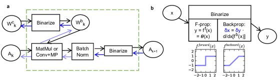
Figure 1: Review of the Courbariaux et al. (2016) BNN Training Algorithm: a. A binary neural network is composed of this binary convolution transformer (dashed green box). Each oval corresponds to a tensor and the derivative of the cost with respect to that tensor. Rectangles correspond to transformers that specify forward and backward propagation functions. Associated with each binary weight, $w^{b}$, is a continuous weight, $w^{c}$, that is used to accumulate gradients. $k$ denotes the $k$th layer of the network. b. Each binarize transformer has a forward function and a backward function. The forward function simply binarizes the inputs. In the backward propagation step, one normally computes the derivative of the cost with respect to the input of a transformer via the Jacobian of the forward function and the derivative of the cost with respect to the output of that transformer ($\delta u\equiv dC/du$ where $C$ is the cost function used to train the network). Since the binarize function is non-differentiable, they use a smoothed version of the forward function for the backward function (in particular, the straight-through estimator of Bengio et al. (2013)).

2 Related Work

Neural networks that achieve good performance on tasks such as IMAGENET object recognition are highly computationally intensive. For instance, AlexNet has 61 million parameters and executes 1.5 billion operations to classify one 224 by 224 image (30 thousand operations/pixel) (Rastegari et al. (2016)). There has been a substantial amount of work to reduce this computational cost for embedded applications.

First, there are a variety of approaches that seek to compress pre-trained networks. Kim et al. (2015) uses a Tucker decomposition of the kernel tensor and fine tunes the network afterwards. Han et al. (2015b) train a network, prune low magnitude connections, and retrain. Han et al. (2015a) extend their previous work to additionally include a weight sharing quantization step and Huffman coding of the weights.

Second, researchers have sought to train networks using either low precision floating point numbers or fixed point numbers, which allow for cheaper multiplications (Courbariaux et al. (2014), Gupta et al. (2015), Judd et al. (2015), Gysel et al. (2016), Lin et al. (2016), Lai et al. (2017)).

Third, there are numerous works on training networks that have quantized weights and or activations. Classically, Bengio et al. (2013) looked at a variety of estimators for the gradient through a stochastic binary unit. Courbariaux et al. (2015) trains networks with binary weights, and then later with binary weights and activations (Courbariaux et al. (2016)). Rastegari et al. (2016) replace a continuous weight matrix with a scalar times a binary matrix (and have a similar approximation for weight activation dot products). Kim & Smaragdis (2016) train a network with weights restricted in the range $-1$ to $1$ and then use a noisy backpropagation scheme train a network with binary weights and activations. Alemdar et al. (2016), Li et al. (2016) and Zhu et al. (2016) focus on networks with ternary weights. Further work seeks to quantize the weights and activations in neural networks to an arbitrary number of bits (Zhou et al. (2016), Hubara et al. (2016)). Zhou et al. (2017) use weights and activations that are zero or powers of two. Lin et al. (2015) and Zhou et al. (2016) quantize backpropagation in addition to the forward propagation.

Beyond merely seeking to compress neural networks, there is a variety of papers that seek to analyze the internal representations of neural networks. Agrawal et al. (2014) found that feature magnitudes in higher layers do not matter (e.g. binarizing features barely changes classification performance). Merolla et al. (2016) analyze the robustness of neural network representations to a collection of different distortions. Dosovitskiy & Brox (2016) observe that binarizing features in intermediate layers of a CNN and then using backpropagation to find an image with those features leads to relatively little distortion of the image compared to dropping out features. These works naturally lead into our work where we are seeking to better understand the representations in neural networks based on the geometry of HD binary vectors.

3 Theory and Experiments

In this section, we outline two theoretical predictions and then verify them experimentally. We train a binary neural network on CIFAR-10 (same learning algorithm and architecture as in Courbariaux et al. (2016)). This convolutional neural network has six layers of convolutions, all of which have a 3 by 3 spatial kernel. The number of feature maps in each layer are 128, 128, 256, 256, 512, 512. After the second, fourth, and sixth convolutions, we do a 2 by 2 max pooling operation. Then we have two fully connected layers with $1024$ units each. Each layer has a batch norm layer in between. We note that the dimension of the weight vector in consideration (i.e. convolution converted to a matrix multiply) is the patch size ($=3*3=9$) times the number of channels. We also carried out experiments using MNIST and got similar results.

3.1 Preservation of Direction During Binarization

In the hyperdimensional computing theory of Kanerva (2009), one of the key ideas is that two random, high-dimensional vectors of dimension $d$ whose entries are chosen uniformly from the set $\{-1,1\}$ are approximately orthogonal (by the central limit theorem, the cosine angle between two such random vectors is normally distributed with $\mu=0$ and $\sigma\sim 1/\sqrt{d}$ ($\cos\theta\approx 0\rightarrow\theta\approx\frac{\pi}{2}$)). We apply this approach of analyzing the geometry (i.e. angle distributions) of high-dimensional vectors to binary vectors. As a null distribution, we use the standard normal distribution, which is rotationally invariant, to generate our vectors. In moderately high dimensions, binarizing a random vector changes its direction by a small amount relative to the angle between two random vectors. This is contrary to our low-dimensional intuition that is guided by the fact that the angle between two random 2D vectors is uniformly distributed (Fig. 2).

In order to test the applicability of our theory of Gaussian random vectors to real neural networks, we train a multilayer binary CNN on CIFAR10 (using the Courbariaux et al. (2016) method) and look at the weight vectors in that trained network. We see a close correspondence between the experimental results and our theory for the angles between the binary and continuous weights (Fig. 2). We note that there is a small but systematic deviation from the theory towards larger angles for the higher layers of the network.

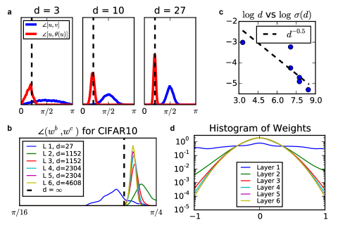
Figure 2: Binarization of Random Vectors Approximately Preserves their Direction: (a) Distribution of angles between two random vectors, and between a vector and its binarized version, for a rotationally invariant distribution. Looking at the angle between a random vector of dimension $d$ and its binarized version, we get the red curves. We note that the distribution is peaked near the $d\rightarrow\infty$ limit of $\arccos\sqrt{2/\pi}\approx 37^{\circ}$ (SI, Sec. 1). Is $37^{\circ}$ a small angle or a large angle? In order to think about that, consider the distribution of angles between two random vectors (blue curves). We see that for low dimensions, the angle between a vector and its binarized version has a high probability of being similar to a pair of two random vectors. However, when we get to a moderately high dimension, we see that the red and blue curves are well separated. (b) Angle distribution between continuous and binary weight vectors by layer for a binary CNN trained on CIFAR-10. For the higher layers, we see a relatively close correspondence with the theory, but with a systematic deviation towards slightly larger angles. $d$ is the dimension of the filters at each layer. (c) Standard deviations of the angle distributions from (b) by layer. We see a correspondence to the theoretical expectation that standard deviations of each of the angle distributions scales as $d^{-0.5}$ (SI, Sec. 1). (d) Histogram of the components of the continuous weights at each layer. We note that this distribution is approximately Gaussian for all but the first layer. Furthermore, we note that there is a high density of weights near zero, which is the threshold for the binarization function.

3.2 Dot Product Preservation as a Sufficient Condition for Sensible Learning Dynamics

One reasonable question to ask is: are these so-called ’continuous weights’ just a learning artifact without a clear correspondence to the binary weights? While we know that $w^{b}=\theta(w^{c})$, there are many continuous weights that map onto a particular binary weight vector. Which one do we find when we apply the method of Courbariaux et al. (2016)? As we discuss below, we get the continuous weight that preserves the dot products with the activations. The key to our analysis is to focus on the transformers in our network whose forward and backward propagation functions are not related in the way that they would normally be related in typical gradient descent.

We show that the modified gradient that we are using can be viewed as an estimator of the true gradient that would be used to train the continuous weights in traditional backpropagation. Furthermore, we show that a sufficient property for this estimator to be a good one is that the dot products of the activations with the pre-binarized and post-binarized weights are proportional.

Suppose we have a neural network where we allocate two tensors, $u$, and $v$ (and the associated derivatives of the cost with respect to those tensors, $\delta u$ and $\delta v$). Suppose that the loss as a function of $v$ is $L(x)|_{x=v}$. Further, there are two potential forward propagation functions, $f$, and $g$. If we trained our network under normal conditions using $g$ as the forward propagation function, then we would compute

$$v\leftarrow g(u)\qquad\delta v\leftarrow L^{\prime}(x=v=g(u))\qquad\delta u\leftarrow\delta v\cdot g^{\prime}(u)$$

In the modified backpropagation scheme, we compute

$$v\leftarrow f(u)\qquad\delta v=L^{\prime}(x=v=f(u))\qquad\delta u\leftarrow\delta v\cdot g^{\prime}(u)$$

A sufficient condition for the updates $\delta u$ to be the same is $L^{\prime}(x=f(u))\sim L^{\prime}(x=g(u))$ where $a\sim b$ means that the vector $a$ is a scalar times the vector $b$.

Now we specialize this argument to the binarize block that binarizes the weights in our networks. Here, $u$ is the continuous weight, $w^{c}$, $f(u)$ is the pointwise binarize function, $g(u)$ is the identity function , and $L$ is the loss of the network as a function of the weights in a particular layer. Given our architecture, we can write $L(x)=M(a\cdot x)$ where $a$ are the activations corresponding to that layer ($a$ is binary for all except the first layer) and $M$ is the loss as a function of the weight-activation dot products. Then $L^{\prime}(x)=M^{\prime}(a\cdot x)\odot a$ where $\odot$ denotes a pointwise multiply. Thus the sufficient condition is $M^{\prime}(a\cdot w^{b})\sim M^{\prime}(a\cdot w^{c})$. Since the dot products are followed by a batch normalization, $M(k\vec{x})=M(\vec{x})\rightarrow M^{\prime}(\vec{x})=kM^{\prime}(k\vec{x})$. Therefore, it is sufficient that

$$a\cdot w^{b}\sim a\cdot w^{c}$$

We call this final relation the Dot Product Preservation (DPP) property. In summary, the learning dynamics where we use $g$ for the forward and backward passes (i.e. training the network with continuous weights) is approximately equivalent to the modified learning dynamics ($f$ on the forward pass, and $g$ on the backward pass) when we have the DPP property.

We also come at this problem from another direction. In SI, Sec. 2 we work out the learning dynamics of the modified backprop scheme in the case of a one layer neural network that seeks to do regression (this ends up being linear regression with binary weights). In this case, the learning dynamics for the weights end up being $\Delta w^{c}\sim C_{yx}-\theta(w^{c})C_{xx}$ where $C_{yx}$ is the input-output correlation matrix and $C_{xx}$ is the input covariance matrix. Since $\theta$ forces the weight matrix to be binary, this equation cannot be satisfied exactly in general conditions. Specializing to the case of an identity input covariance matrix, we show that $E(\theta(w^{c}))=C_{yx}$. Intuitively, the entries of the weight matrix oscillate between $+1$ and $-1$ in the correct proportion in order to get the weight matrix correct in expectation. In high dimensions, these are likely to be out of phase, leading to a low variance estimator.

Indeed, in our numerical experiments on CIFAR10, we see that the dot products of the activations with the pre-binarization and post-binarization weights are highly correlated (Fig. 3). Likewise, we verify a second relation that corresponds to ablating the other instance of binarize transformer in the network, the transformer that binarizes the activations : $w^{b}\cdot a^{c}\sim w^{b}\cdot a^{b}$ where $a^{c}$ denotes the pre-binarized (post-batch norm) activations (Fig. 4). For the practitioner, we recommend checking the DPP property in order to assess the areas in which the network’s performance is being degraded by the compression of the weights or activations.

Impact on Classification: As we’ve argued, the quantity that the network cares about, the batch normalized weight-activation dot products, is preserved under binarization of the weights. It is also natural to ask to what extent the classification performance depends on the binarization of the weights. In our experiments on CIFAR10, if we remove the binarization of the weights on all of the convolutional layers, the classification performance drops by only $3$ percent relative to the original network. Looking at each layer individually, we see that removing the weight binarization for the first layer accounts for this entire percentage, and removing the binarization of the weights for each other layer causes no degradation in performance. We note that removing the binarization of the activations unsurprisingly has a substantial impact on the classification performance because that removes the main non-linearity of the network.

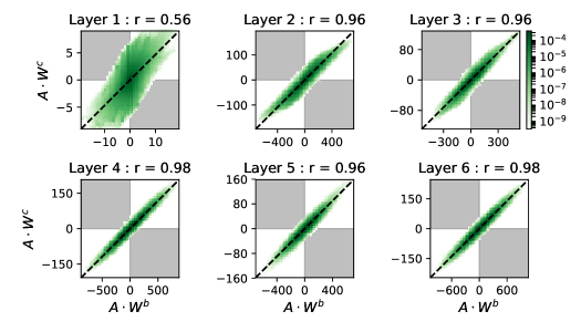
Figure 3: Binarization Preserves Dot Products: In this figure, we verify our hypothesis that binarization approximately preserves the dot-products that the network uses for computations. We train a convolutional neural network on CIFAR-10. Each figure shows a 2d histogram of the dot products between the binarized weights and the activations (horizontal axis) and the dot products between the continuous weights and the activations (vertical axis). Note the logarithmic color scaling. We see that these dot products are highly correlated, verifying our theory ($r$ is the Pearson correlation coefficient). Note they may differ up to a scaling constant due to the subsequent batch norm layer. The top left figure (labeled as Layer 1) corresponds to the input and the first convolution. Note that the correlation is weaker in the first layer. The shaded quadrants correspond to dot products where the sign changes when replacing the binary weights with the continuous weights. Notice that for all but the first layer, a very small fraction of the dot products lie in these off diagonal quadrants.

3.3 Permutation of Activations Reveals Fundamental Difference Between First Layer and Subsequent Layers

Looking at the correlations in Fig. 3, we see that the first layer has a much smaller dot product correlation than the other layers. In order to understand this observation better, we investigate the different factors that lead to the dot product correlation. For instance, it could be the case that the correlation between the two dot products is due to the two weight vectors being closely aligned. Another explanation is that the weight vectors are well-aligned with the informative directions in the data. To study this, we apply a random permutation to the activations in order to generate a distribution with the same marginal statistics as the original data but independent joint statistics. Such a transformation gives us a distribution with a correlation equal to the normalized dot product of the weight vectors (SI Sec. 3). As we can see in Fig. 4, the correlations for the higher layers decrease substantially but the correlation in the first layer increases (for the first layer, the shuffling operation randomly permutes the pixels in the image). Thus we demonstrate that the binary weight vectors in the first layer are not well-aligned with the continuous weight vectors relative to the input data.

We hypothesize that the core issue at play is that the input data is not randomly oriented relative to the axes of binarization. In order to be clear on what we mean by the axes of binarization, first consider the Generalized Binarization Transformation (GBT):

$$\theta_{R}(x)=R^{T}\theta(Rx)$$

where $x$ is a column vector, $R$ is a rotation matrix, and $\theta$ is the pointwise binarization function from before. We call the rows of $R$ the axes of binarization. If $R$ is the identity matrix, then we reduce back to our original binarization function and the axes of binarization are just the canonical basis vectors $(...,0,1,0,...)$. Consider the 27 dimensional input to the first set of convolutions in our network: 3 color channels of a 3 by 3 patch of an image from CIFAR10 with the mean removed. 3 PCs capture 90 percent of the variance of this data and 4 PCs capture 94.5 percent of the variance. Furthermore, these PCs aren’t randomly oriented relative to the binarization axes. For instance, the first two PCs are spatially uniform colors. More generally, natural images (such as those in IMAGENET) will have the same issue. Translation invariance of the pixel covariance matrix implies that the principal components are the filters of the 2D fourier transform. Scale invariance implies a $1/f^{2}$ power spectrum, which results in the largest PCs corresponding to low frequencies.

Stepping back, this control gives us important insight: the first layer is fundamentally different from the other layers due to the non-random orientation of the data relative to the axes of binarization. Practically speaking, we have two recommendations. First, we recommend an architecture that uses a set of continuous convolutional weights to embed images in a high-dimensional binary space, after which it can be manipulated efficiently using binary vectors. While there isn’t a large accuracy degradation on CIFAR10, these observations are going to be more important on datasets with larger images such as IMAGENET. We note that this theoretically grounded recommendation is consistent with previous empirical work. Han et al. (2015b) find that compressing the first set of convolutional weights of a particular layer by the same fraction has the highest impact on performance if done on the first layer. Zhou et al. (2016) find that accuracy degrades by about 0.5 to 1 percent on SHVN when quantizing the first layer weights. Second, we recommend experimenting with a GBT where the rotation is chosen so that it can be computed efficiently. This solves the problem of low-dimensional data embedded in a high dimensional space that is not randomly oriented relative to the binarization function.

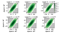
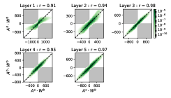
Figure 4: Left: Permuting the activations shows that the correlations observed in Fig. 3 are not merely due to correlations between the binary and continuous weight vectors. The correlations are due to these weight vectors corresponding to important directions in the data. Right: Activation Binarization Preserves Dot Products: Each figure shows a 2d histogram of the dot products between the binarized weights and binarized activations (vertical axis) and post-batch norm (but pre activation binarization) activations (horizontal axis). Again, we see that the binarization transformer does little to corrupt the dot products between weights and activations.

4 Conclusion

Neural networks with binary weights and activations have similar performance to their continuous counterparts with substantially reduced execution time and power usage. We provide an experimentally verified theory for understanding how one can get away with such a massive reduction in precision based on the geometry of HD vectors. First, we show that binarization of high-dimensional vectors preserves their direction in the sense that the angle between a random vector and its binarized version is much smaller than the angle between two random vectors (Angle Preservation Property). Second, we take the perspective of the network and show that binarization approximately preserves weight-activation dot products (Dot Product Preservation Property). More generally, when using a network compression technique, we recommend looking at the weight activation dot product histograms as a heuristic to help localize the layers that are most responsible for performance degradation. Third, we discuss the impacts of the low effective dimensionality on the first layer of the network and recommend either using continuous weights for the first layer or a Generalized Binarization Transformation. Such a transformation may be useful for architectures like LSTMs where the update for the hidden state declares a particular set of axes to be important (e.g. by taking the pointwise multiply of the forget gates with the cell state). More broadly speaking, our theory is useful for analyzing a variety of neural network compression techinques that transform the weights, activations or both to reduce the execution cost without degrading performance.

Acknowledgments

The authors would like to thank Bruno Olshausen, Urs Köster, Spencer Kent, Eric Dodds, Dylan Paiton, and members of the Redwood Center for useful feedback on this work. This material is based upon work supported by the National Science Foundation under Grant No. DGE 1106400 (AGA). Any opinions, findings, and conclusions or recommendations expressed in this material are those of the author(s) and do not necessarily reflect the views of the National Science Foundation. This work was supported in part by Systems on Nanoscale Information fabriCs (SONIC), one of the six SRC STARnet Centers, sponsored by MARCO and DARPA (AGA).

5 Supplementary Information

5.1 Expected Angles

We draw random $n$ dimensional vectors from a rotationally invariant distribution and compare the angles between two random vectors and the binarized version of that vector. We note that a rotationally invariant distribution can be factorized into a pdf for the magnitude of the vector times a distribution on angles. In the expectations that we are calculating, the magnitude cancels out and there is only one rotationally invariant distribution on angles. Thus it suffices to compute these expectations using a Gaussian.

Lemmas:

1. Consider a vector, $v$, chosen from a standard normal distribution of dimension $n$. Let $\rho=\frac{v_{1}}{\sqrt{v_{1}^{2}+...+v_{n}^{2}}}$. Then $\rho$ is distributed according to: $g(\rho)=\frac{1}{\sqrt{\pi}}\frac{\Gamma(n/2)}{\Gamma((n-1)/2)}(1-\rho^{2})^{\frac{n-3}{2}}$ http://www-stat.wharton.upenn.edu/~tcai/paper/Coherence-Phase-Transition.pdf where $\Gamma$ is the Gamma function.

2. $\frac{\Gamma(z+\alpha)}{\Gamma(z+\beta)}=z^{\alpha-\beta}\left(1+\frac{(\alpha-\beta)(\alpha+\beta+1)}{2z}\right)+O(|z|^{-2})$ as $z\rightarrow\infty$

• Distribution of angles between two random vectors.

  Since a Gaussian is a rotationally invariant distribution, we can say without loss of generality that one of the vectors is $(1,0,0,\ldots 0)$. Then the cosine angle between those two vectors is $\rho$ as defined above. While we have the exact distribution, we note that

  • $E(\rho)=0$ due to the symmetry of the distribution.

  • $Var(\rho)=E(\rho^{2})=\frac{1}{n}$ because $1=E\left(\frac{\sum_{i}x_{i}^{2}}{\sum_{j}x_{j}^{2}}\right)=\sum_{i}E\left(\frac{x_{i}^{2}}{\sum_{j}x_{j}^{2}}\right)=n*E(\rho^{2})$

• Angles between a vector and the binarized version of that vector, $\eta=\frac{v\cdot\theta(v)}{||v||\cdot||\theta(v)||}=\frac{\sum_{i}|v_{i}|}{\sqrt{\sum v_{i}^{2}}*\sqrt{n}}$

  • $$E(\eta)=\frac{\sqrt{n}}{\sqrt{\pi}}*\frac{\Gamma(n/2)}{\Gamma((n+1)/2)}\qquad\lim_{n\rightarrow\infty}E(\eta)=\sqrt{\frac{2}{\pi}}$$

    First, we note $E(\eta)=\sqrt{n}E(|\rho|)$. Then $E(|\rho|)=\int_{0}^{1}d\rho\,\rho\frac{2}{\sqrt{\pi}}\frac{\Gamma(n/2)}{\Gamma((n-1)/2)}(1-\rho^{2})^{\frac{n-3}{2}}=\frac{2}{\sqrt{\pi}}*\frac{1}{n-1}\frac{\Gamma(n/2)}{\Gamma((n-1)/2)}$ (substitute $u=\rho^{2}$ and use $\Gamma(x+1)=x\Gamma(x)$ ). Lemma two gives the $n\rightarrow\infty$ limit.

  • $$Var(\eta)=\frac{1}{n}\left(1-\frac{1}{\pi}\right)+O(1/n^{2})$$

    Thus we have the normal scaling as in the central limit theorem of the large $n$ variance. We can calculate this explicitly following the approach of https://en.wikipedia.org/wiki/Volume_of_an_n-ball#Gaussian_integrals.

    As we’ve calculated $E(\eta)$, it suffices to calculate $E(\eta^{2})$. Expanding out $\eta^{2}$, we get $E(\eta^{2})=\frac{1}{n}+(n-1)*E(\frac{|v_{1}v_{2}|}{v_{1}^{2}+\ldots v_{n}^{2}})$. Below we show that $E(\frac{|v_{1}v_{2}|}{v_{1}^{2}+\ldots v_{n}^{2}})=\frac{2}{\pi n}$. Thus the variance is:

    $$\frac{1}{n}*\left(1-\frac{2}{\pi}\right)+\frac{2}{\pi}-\left(\frac{\sqrt{n}}{\sqrt{\pi}}\frac{\Gamma(n/2)}{\Gamma((n+1)/2)}\right)^{2}$$

    Using Lemma 2 to expand out the last term, we get $[\frac{\sqrt{n}}{\sqrt{\pi}}(n/2)^{-1/2}(1-1/(4n)+O(n^{-2}))]^{2}$ = $\frac{2}{\pi}(1-1/(2n)+O(n^{-2}))$. Plugging this in gives the desired result.

    Going back to the calculation of that expectation, change variables to $v_{1}=r\cos\theta$, $v_{2}=r\sin\theta$, $z^{2}=v_{3}^{2}+...+v_{n}^{2}$. The integration over the volume element $dv_{3}\ldots dv_{n}$ is rewritten as $dzdA_{n-3}$ where $dA_{n}$ denotes the surface element of a $n$ sphere. Since the integrand only depends on the magnitude, $z$, $\int dA_{n-3}=z^{n-3}*S_{n-3}$ where $S_{n}=\frac{2\pi^{(n+1)/2}}{\Gamma(\frac{n+1}{2})}$ denotes the surface area of a unit $n$-sphere. Then

    $$E\left(\frac{|v_{1}v_{2}|}{v_{1}^{2}+\ldots v_{n}^{2}}\right)=(2\pi)^{-n/2}S_{n-3}\int_{0}^{2\pi}d\theta|\cos\theta\sin\theta|*\int rdrz^{n-3}dz*\frac{r^{2}}{r^{2}+z^{2}}*e^{-(z^{2}+r^{2})/2}$$

    Then substitute $r=p\cos\phi$, $z=p\sin\phi$ where $\phi\in[0,\pi/2]$

    $$=(2\pi)^{-n/2}*2S_{n-3}\int_{0}^{\pi/2}d\phi\cos\phi^{3}*\sin\phi^{n-3}\int_{0}^{\infty}dp*p^{n-1}e^{-p^{2}/2}$$

    The first integral is $\frac{2}{n(n-2)}$ using $u=\sin^{2}\phi$. The second integral is $2^{(n-2)/2}\Gamma(n/2)$ using $u=p^{2}/2$ and the definition of the gamma function. Simplifying, we get $\frac{2}{\pi*n}$.

Roughly speaking, we can see that the angle between a vector and a binarized version of that vector converges to $\arccos\sqrt{\frac{2}{\pi}}\approx 37^{\circ}$ which is a very small angle in high dimensions.

5.2 An Explicit Example of Learning Dynamics

In this subsection, we look at the learning dynamics for the BNN training algorithm in a simple case and gain some insight about the learning algorithm. Consider the case of regression where we try and predict $y$ with $x$ with a binary linear predictor. Using a squared error loss, we have $L=(y-\hat{y})^{2}=(y-w^{b}x)^{2}=(y-\theta(w^{c})x)^{2}$. (In this notation, $x$ is a column vector.) Taking the derivative of this loss with respect to the continuous weights and using the rule for back propagating through the binarize function, we get $\Delta w^{c}\sim-dL/dw^{c}=-dL/dw^{b}\cdot dw^{b}/dw^{c}=(y-w^{b}x)x^{T}$. Finally, averaging over the training data, we get

$$\Delta w^{c}\sim C_{yx}-\theta(w^{c})\cdot C_{xx}\qquad C_{yx}=E[yx^{T}]\qquad C_{xx}=E(xx^{T})$$ (1)

It is worthwhile to compare this equation the corresponding equation from typical linear regression: $\Delta w^{c}\sim C_{yx}-w^{c}\cdot C_{xx}$ For simplicity, lets consider the case where $C_{xx}$ is the identity matrix. In this case, all of the components of $w$ become independent and we get the equation $\delta w=\epsilon*(\alpha-\theta(w))$ where $\epsilon$ is the learning rate and $\alpha$ is the entry of $C_{yx}$ corresponding to a particular element, $w$. If we were doing regular linear regression, it is clear that the stable point of these equations is when $w=\alpha$. Since we binarize the weight, that equation cannot be satisfied. However, it can be shown $(\star)$ that in this special case of binary weight linear regression, $E(\theta(w^{c}))=\alpha$.

Intuitively, if we consider a high dimensional vector and the fluctuations of each component are likely to be out of phase, then $w^{b}\cdot x\approx w^{c}\cdot x$ is going to be correct in expectation with a variance that scales as $\frac{1}{n}$. During the actual learning process, we anneal the learning rate to a very small number, so the particular state of a fluctuating component of the vector is frozen in. Relatedly, the equation $C_{yx}\approx wC_{xx}$ is easier to satisfy in high dimensions, whereas in low dimensions, we only satisfy it in expectation.

Rough proof for $(\star)$: Suppose that $|\alpha|\leq 1$. The basic idea of these dynamics is that you are taking steps of size proportional to $\epsilon$ whose direction depends on whether $w>0$ or $w<0$. In particular, if $w>0$, then we take a step $-\epsilon\cdot|1-\alpha|$ and if $w<0$, we take a step $\epsilon\cdot(\alpha+1)$. It is evident that after a sufficient burn-in period, $|w|\leq\epsilon*\max(|1-\alpha|,1+\alpha)\leq 2\epsilon$. Suppose $w>0$ occurs with fraction $p$ and $w<0$ occurs with fraction $1-p$. In order for $w$ to be in equilibrium, oscillating about zero, we must have that these steps balance out on average: $p(1-\alpha)=(1-p)(1+\alpha)\rightarrow p=(1+\alpha)/2$. Then the expected value of $\theta(w)$ is $1*p+(-1)*(1-p)=\alpha$. When $|\alpha|>1$, the dynamics diverge because $\alpha-\theta{bin}(w)$ will always have the same sign. This divergence demonstrates the importance of some normalization technique such as batch normalization or attempting to represent $w$ with a constant times a binary matrix.

5.3 Dot Product Correlations After Activation Permutation

Suppose that we look at $A=w\cdot a$ and $B=v\cdot a$ where $a$ are now the randomly permuted activations. What does the distribution of $A,B$ look like? To answer this, we look at the correlation between $A$ and $B$ and show that it is the correlation between $w$ and $v$. First, let us assume that $p(a)=\prod_{i}f(a_{i})$ $E(a_{i})=0$, $E(a_{i}^{2})=\sigma^{2}$. Then $E(A)=E(B)=0$. Now we compute:

$E(AB)=\sum_{i,j}w_{i}v_{j}E(a_{i}a_{j})=\sigma^{2}(w\cdot v)$ Likewise, $E(A^{2})=\sigma^{2}(w\cdot w)$ and $E(B^{2})=\sigma^{2}(v\cdot v)$. Thus the correlation coefficient $\frac{w\cdot v}{|w||v|}$, as desired

References

- Agrawal et al. (2014) Pulkit Agrawal, Ross Girshick, and Jitendra Malik. Analyzing the performance of multilayer neural networks for object recognition. In European Conference on Computer Vision, pp. 329–344. Springer, 2014.
- Alemdar et al. (2016) Hande Alemdar, Nicholas Caldwell, Vincent Leroy, Adrien Prost-Boucle, and Frédéric Pétrot. Ternary neural networks for resource-efficient ai applications. arXiv preprint arXiv:1609.00222, 2016.
- Andri et al. (2017) Renzo Andri, Lukas Cavigelli, Davide Rossi, and Luca Benini. Yodann: An architecture for ultra-low power binary-weight cnn acceleration. IEEE Transactions on Computer-Aided Design of Integrated Circuits and Systems, 2017.
- Bengio et al. (2013) Yoshua Bengio, Nicholas Léonard, and Aaron Courville. Estimating or propagating gradients through stochastic neurons for conditional computation. arXiv preprint arXiv:1308.3432, 2013.
- Courbariaux et al. (2014) Matthieu Courbariaux, Yoshua Bengio, and Jean-Pierre David. Training deep neural networks with low precision multiplications. arXiv preprint arXiv:1412.7024, 2014.
- Courbariaux et al. (2015) Matthieu Courbariaux, Yoshua Bengio, and Jean-Pierre David. Binaryconnect: Training deep neural networks with binary weights during propagations. In Advances in Neural Information Processing Systems, pp. 3123–3131, 2015.
- Courbariaux et al. (2016) Matthieu Courbariaux, Itay Hubara, Daniel Soudry, Ran El-Yaniv, and Yoshua Bengio. Binarized neural networks: Training neural networks with weights and activations constrained to +1 and -1. arXiv preprint arXiv:1602.02830, 2016.
- Dosovitskiy & Brox (2016) Alexey Dosovitskiy and Thomas Brox. Inverting visual representations with convolutional networks. In Proceedings of the IEEE Conference on Computer Vision and Pattern Recognition, pp. 4829–4837, 2016.
- Esser et al. (2016) Steven K Esser, Paul A Merolla, John V Arthur, Andrew S Cassidy, Rathinakumar Appuswamy, Alexander Andreopoulos, David J Berg, Jeffrey L McKinstry, Timothy Melano, Davis R Barch, et al. Convolutional networks for fast, energy-efficient neuromorphic computing. Proceedings of the National Academy of Sciences, pp. 201604850, 2016.
- Gupta et al. (2015) Suyog Gupta, Ankur Agrawal, Kailash Gopalakrishnan, and Pritish Narayanan. Deep learning with limited numerical precision. In ICML, pp. 1737–1746, 2015.
- Gysel et al. (2016) Philipp Gysel, Mohammad Motamedi, and Soheil Ghiasi. Hardware-oriented approximation of convolutional neural networks. arXiv preprint arXiv:1604.03168, 2016.
- Han et al. (2015a) Song Han, Huizi Mao, and William J Dally. Deep compression: Compressing deep neural networks with pruning, trained quantization and huffman coding. arXiv preprint arXiv:1510.00149, 2015a.
- Han et al. (2015b) Song Han, Jeff Pool, John Tran, and William Dally. Learning both weights and connections for efficient neural network. In Advances in Neural Information Processing Systems, pp. 1135–1143, 2015b.
- Hubara et al. (2016) Itay Hubara, Matthieu Courbariaux, Daniel Soudry, Ran El-Yaniv, and Yoshua Bengio. Quantized neural networks: Training neural networks with low precision weights and activations. arXiv preprint arXiv:1609.07061, 2016.
- Judd et al. (2015) Patrick Judd, Jorge Albericio, Tayler Hetherington, Tor Aamodt, Natalie Enright Jerger, Raquel Urtasun, and Andreas Moshovos. Reduced-precision strategies for bounded memory in deep neural nets. arXiv preprint arXiv:1511.05236, 2015.
- Kanerva (2009) Pentti Kanerva. Hyperdimensional computing: An introduction to computing in distributed representation with high-dimensional random vectors. Cognitive Computation, 1(2):139–159, 2009.
- Kim & Smaragdis (2016) Minje Kim and Paris Smaragdis. Bitwise neural networks. arXiv preprint arXiv:1601.06071, 2016.
- Kim et al. (2015) Yong-Deok Kim, Eunhyeok Park, Sungjoo Yoo, Taelim Choi, Lu Yang, and Dongjun Shin. Compression of deep convolutional neural networks for fast and low power mobile applications. arXiv preprint arXiv:1511.06530, 2015.
- Lai et al. (2017) Liangzhen Lai, Naveen Suda, and Vikas Chandra. Deep convolutional neural network inference with floating-point weights and fixed-point activations. arXiv preprint arXiv:1703.03073, 2017.
- Li et al. (2016) Fengfu Li, Bo Zhang, and Bin Liu. Ternary weight networks. arXiv preprint arXiv:1605.04711, 2016.
- Lin et al. (2016) Darryl Lin, Sachin Talathi, and Sreekanth Annapureddy. Fixed point quantization of deep convolutional networks. In International Conference on Machine Learning, pp. 2849–2858, 2016.
- Lin et al. (2015) Zhouhan Lin, Matthieu Courbariaux, Roland Memisevic, and Yoshua Bengio. Neural networks with few multiplications. arXiv preprint arXiv:1510.03009, 2015.
- Merolla et al. (2016) Paul Merolla, Rathinakumar Appuswamy, John Arthur, Steve K Esser, and Dharmendra Modha. Deep neural networks are robust to weight binarization and other non-linear distortions. arXiv preprint arXiv:1606.01981, 2016.
- Neftci et al. (2016) Emre Neftci, Charles Augustine, Somnath Paul, and Georgios Detorakis. Neuromorphic deep learning machines. arXiv preprint arXiv:1612.05596, 2016.
- Rastegari et al. (2016) Mohammad Rastegari, Vicente Ordonez, Joseph Redmon, and Ali Farhadi. Xnor-net: Imagenet classification using binary convolutional neural networks. arXiv preprint arXiv:1603.05279, 2016.
- Zeiler & Fergus (2014) Matthew D Zeiler and Rob Fergus. Visualizing and understanding convolutional networks. In European conference on computer vision, pp. 818–833. Springer, 2014.
- Zhou et al. (2017) Aojun Zhou, Anbang Yao, Yiwen Guo, Lin Xu, and Yurong Chen. Incremental network quantization: Towards lossless cnns with low-precision weights. arXiv preprint arXiv:1702.03044, 2017.
- Zhou et al. (2016) Shuchang Zhou, Yuxin Wu, Zekun Ni, Xinyu Zhou, He Wen, and Yuheng Zou. Dorefa-net: Training low bitwidth convolutional neural networks with low bitwidth gradients. arXiv preprint arXiv:1606.06160, 2016.
- Zhu et al. (2016) Chenzhuo Zhu, Song Han, Huizi Mao, and William J Dally. Trained ternary quantization. arXiv preprint arXiv:1612.01064, 2016.