Heliospheric modulation of cosmic rays during the neutron monitor era: Calibration using PAMELA data for 2006–2010

Abstract

A new reconstruction of the heliospheric modulation potential for galactic cosmic rays is presented for the neutron monitor era, since 1951. The new reconstruction is based on an updated methodology in comparison to previous reconstructions: (1) the use of the new-generation neutron monitor yield function; (2) the use of the new model of the local interstellar spectrum, employing in particular direct data from the distant missions; and (3) the calibration of the neutron monitor responses to direct measurements of the cosmic ray spectrum performed by the PAMELA space-borne spectrometer over 47 time intervals during 2006–2010. The reconstruction is based on data from six standard NM64-type neutron monitors (Apatity, Inuvik, Kergulen, Moscow, Newark and Oulu) since 1965, and two IGY-type ground-based detectors (Climax and Mt.Washington) for 1951–1964. The new reconstruction, along with the estimated uncertainties is tabulated in the paper. The presented series forms a benchmark record of the cosmic ray variability (in the energy range between 1–30 GeV) for the last 60 years, and can be used in long-term studies in the fields of solar, heliospheric and solar-terrestrial physics.

Gindraft=false USOSKIN ET AL. Modulation potential for NM era Corresponding author: I. Usoskin

1 Introduction

Galactic cosmic rays (GCR) is a population of energetic, mostly nucleonic, with a small fraction of electrons and positrons, particles permanently bombarding Earth and forming the radiation environment in the near-Earth space and in the atmosphere (Vainio et al., 2009). The flux of GCR is modulated, in the low-energy (below 100 GeV) part of the spectrum, by solar magnetic activity over the solar cycle (Potgieter, 2013). The variability of the GCR flux is constantly monitored by the network of ground-based neutron monitors (NMs) since the 1950s. Because of the thickness of the Earth’s atmosphere and the shielding effect of the geomagnetic field, ground-based measurements have to be translated into the actual flux units beyond the atmosphere and magnetosphere by applying a complicated transport model. On the other hand, GCR energy spectra are occasionally measured in the energy range exceeding 1 GeV by balloon-borne or space-borne detectors providing a direct way to calibrate the ground-based detectors and to link NM data to the real GCR spectra. The most important in this respect are the long-running experiments PAMELA (Payload for Antimatter Matter Exploration and Light-nuclei Astrophysics) (Adriani et al., 2013) and AMS-02 (Alpha Magnetic Spectrometer) (Aguilar et al., 2015), operating for the last decade. Before that, only balloon-borne detectors (and a short test flight of AMS-01 in 1998 (Alcaraz et al., 2000)) were operating in this energy range.

For many practical purposes it is ueful to describe the GCR energy spectrum near Earth by the force-field approximation (e.g. Gleeson and Axford, 1968; Caballero-Lopez and Moraal, 2004) with its single formal parameter – the modulation potential $\phi$ (see formalism in Usoskin et al., 2005). We note that the force-field approximation is not validated as a physical model of GCR modulation, and the modulation potential has no clear physical meaning (often used interpretation of the mean adiabatic energy loss is not exactly correct (see, e.g. Caballero-Lopez and Moraal, 2004)). On the other hand, it provides a handy empirical description of the actual shape of the GCR energy spectrum near Earth which, while not making a claim to explain the modulation process, offers a simple single-value parametrization of the GCR spectrum for many practical purposes, such as atmospheric ionization and climate modeling, radiation environment, cosmogenic radionuclide studies, assessments of radiation hazard risks, etc. A model allowing one to estimate the variability of the modulation potential in time was proposed by Usoskin et al. (2005) based on the data from the world NM network. That work led to a systematic reconstruction of monthly $\phi$ values since the 1950s. Calibration to the direct GCR measurements was done using the space-borne AMS-01 data for moderate solar activity and MASS89 balloon-borne data (Webber et al., 1991) for high solar activity. This work was extended by Usoskin et al. (2011) by including a more realistic GCR composition (heavier species were considered).

Here we revisit the reconstruction of the modulation potential along three main directions:

1. The earlier models were based upon previous generations of the NM yield functions (Debrunner et al., 1982; Clem and Dorman, 2000; Matthiä et al., 2009) that were unable to reproduce the exact count rate of individual NMs and the shape of the latitudinal survey (Caballero-Lopez and Moraal, 2012). By contrast, here we use the new-generation NM yield function (Mishev et al., 2013, see also erraturm therein), which agrees, for the first time, with the actual measurements of the NM count rates and observational surveys (Gil et al., 2015).

2. While the earlier models were based upon an estimate of the local interstellar spectrum (LIS) by Burger et al. (2000) for earlier models such as (Garcia-Munoz et al., 1975), here we use a recent estimate of the LIS by Vos and Potgieter (2015) who revised the LIS by using precise measurements from AMS-02 and PAMELA space-borne detectors and considering also Voyager data beyond the heliospheric termination shock, not available until recently.

3. Earlier models were based upon a calibration method using only two directly measured GCR spectra: MASS89 and AMS-01. Here we use a newly available GCR spectra precisely measured by the PAMELA instrument (Adriani et al., 2013) during 47 time intervals during 2006 – 2010.

We note that with these modifications (especially the new LIS and calibration), the values of $\phi$ calculated here are not directly comparable with the earlier reconstructions.

In Section 2 we describe the formalism of the model and the used LIS. The PAMELA data used for calibration are introduced in Section 3. Selection and calibration of the NMs are explained in Section 4. The reconstruction of the modulation potential is described in Section 5 and discussed in Section 6. Our conclusions are presented in Section 7.

2 Formalism

Here we use the established formalism of representing the counting rate of a NM at any location and time $t$, as an integral of the product of the cosmic ray energy spectrum and the specific yield function of the NM:

$$N(h,t)=\kappa\sum_{i}\int_{T_{c_{i}}}^{\infty}Y_{i}(T,h)\cdot J_{i}(T,t)\,dT,$$ (1)

where $N$ is the count rate of a NM reduced to the standard barometric pressure, $J_{i}(T,t)$ is the energy spectrum of the $i-$th specie of GCR nuclei outside the Earth’s magnetosphere and atmosphere, $Y_{i}(T,h)$ is the specific yield function of a NM, $T$ is kinetic energy of the primary cosmic rays particle, $h$ is height (atmospheric depth at the NM location), and $\kappa$ accounts for the “non-ideality” of a NM (see Section 4). The yield function, corresponding to the standard sea-level 6NM64, was taken according to a recent simulation (Mishev et al., 2013, see also erratum therein). Integration is performed above the kinetic energy $T_{c}$ corresponding to the geomagnetic cutoff rigidity $P_{c}$ in the location of the NM. The yield function includes both development of the atmospheric cascade with different types of secondary particles and the response of a detector to the secondary particles (Clem and Dorman, 2000; Mishev et al., 2013; Aiemsa-ad et al., 2015).

In order to describe the GCR differential energy spectrum near Earth we employed the widely used force-field approximation (e.g. Vainio et al., 2009):

$$J_{i}(T)=J_{{\rm LIS}_{i}}(T+\Phi_{i})\frac{T^{2}-T^{2}_{r}}{(T+\Phi_{i})^{2}-T^{2}_{r}}$$ (2)

where $J_{{\rm LIS}_{i}}$ is the LIS, $T_{r}=0.938$ GeV is the proton’s rest mass, $\Phi_{i}$ is the mean energy loss of the GCR particle inside the heliosphere, as defined by the modulation potential $\phi$: $\Phi_{i}=\phi\cdot(eZ_{i}/A_{i})$, where $Z_{i}$ and $A_{i}$ are the charge and mass numbers of the nucleus of type $i$. Here we use the LIS from Vos and Potgieter (2015), which is a new parameterization based on both near-Earth and distant (beyond the heliospheric termination shock) measurements of GCR spectra and compositions. The LIS takes the following form for protons:

$$J_{\rm LIS}=2.7\cdot 10^{3}\,\,{T^{1.12}\over\beta^{2}}\left({T+0.67\over 1.67}\right)^{-3.93},$$ (3)

where $\beta=v/c$ is the ratio of the proton’s velocity to the speed of light, $J$ and $T$ are given in [m² sec sr GeV/nuc]^-1 and GeV/nucleon, respectively. This LIS is shown in Fig. 1. We note that there are some other recent LIS estimates (e.g., Potgieter et al., 2014; Cummings et al., 2016) which differ from each other mostly in the low energy part. In order to account for that, Corti et al. (2016) proposed an additional parameter describing modulation for GCR protons with energy below 125 MeV, to which NMs are however insensitive.

It is important to consider $\alpha-$particles (effectively including heavier species) separately from protons since they are modulated differently and contribute 30–50% to the overall count rate of a NM (Usoskin et al., 2011; Caballero-Lopez and Moraal, 2012). For $\alpha-$particles (including the heavier species) we used the same form as for protons (Eq. 3) but with the weight of 0.3 (in the number of nucleons) similarly to Usoskin et al. (2011). The intensity in this case is given for nucleons, and kinetic energy in GeV/nuc.

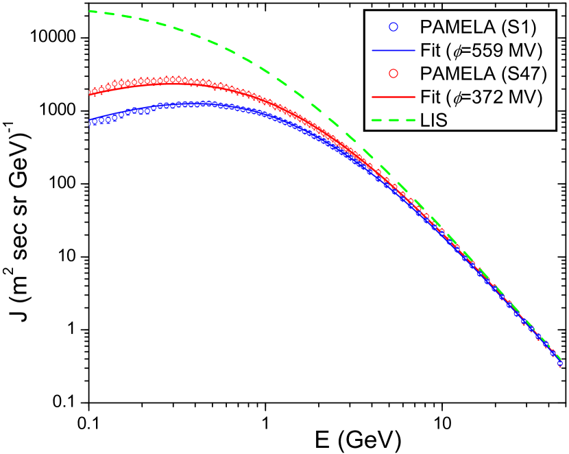
Figure 1: Examples of the fits (curves) of the GCR proton spectra measured by PAMELA (dots with errors bars) for period S1 (07.07.2006–26.07.2006, blue) and S47 (02.01.2010–23.01.2010, red). Green dashed line denotes the considered LIS (Equation 3).

3 PAMELA data

The data used here include direct measurements of GCR energy spectra by the PAMELA space mission (Adriani et al., 2011), which is a space-borne magnetic spectrometer installed onboard the low orbiting satellite Resurs-DK1 with a quasi-polar (inclination $70^{\circ}$) elliptical orbit (height 350–600 km). PAMELA was in operation since Summer 2006 through January 2016 continuously measuring all charged energetic ($>80$ MeV) particles in space.

Here we make use of PAMELA the measurements of the differential energy spectra of CR protons obtained between July 2006 and January 2010, during which time the solar activity varied between moderate and very low. This period was divided into 47 unequal time intervals, and the measured proton energy spectrum were provided by Adriani et al. (2013) (digital data are available at http://tools.asdc.asi.it/cosmicRays.jsp?tabId=0). The month of December 2006 was excluded from consideration because of large disturbances of the CR flux due to a major Forbush decrease and a ground level enhancement #70 (Usoskin et al., 2015).

Each measured proton spectrum was fitted with the force-field model (Eqs. 2 – 3). The best-fit value of $\phi$ and its $1\sigma$ uncertainties were found for each time interval by minimizing $\chi^{2}-$statistics in the interval of energies between 1–30 GeV, which corresponds to the most effective energy of GCR detection by NMs. Two examples of the fit are shown in Fig. 1 for time intervals S1 and S47. The obtained values of the modulation potential are shown in Fig. 2.

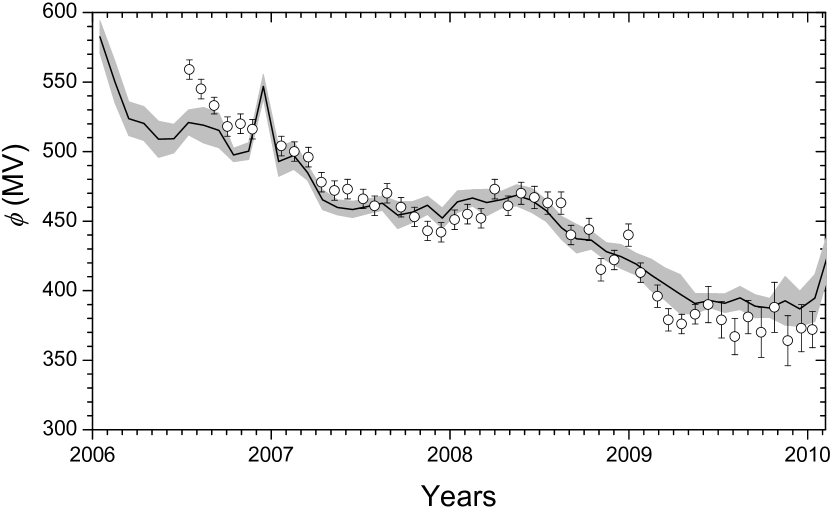
Figure 2: The modulation potential $\phi$, along with its $1\sigma$ uncertainties, during 2006–2009, as obtained from PAMELA measurements (dots with error bars) as well as reconstructed from NM data (black line with grey shading). The spike in the curve corresponds to December 2006.

4 Selection and calibration of NMs

Although the formalism (Section 2) provides a full theoretical basis to the model count rate of an ideal standard NM, real instruments are neither “ideal” nor perfectly standard: different surrounding structures, instrumental setups (e.g., the electronic dead-time, high voltage, number of counters, the material for moderator, etc.), type of the counter (Soviet/Russian analogs CNM-15 are about 15% less effective than the standard BP28(NM64) counters, (Gil et al., 2015)), etc., making their sensitivities slightly different from each other. Another source of the difference is that the reference barometric pressure can be set differently for different NMs, which can also result in the count rate being systematically deviating from the modeled one. One approach to deal with that is to perform direct Monte-Carlo simulation of every NM considering the detailed geometry and environment (e.g., Aiemsa-ad et al., 2015; Mangeard et al., 2016). However, it is hardly possible to perform such detailed simulations for all NMs. Accordingly, we consider this uncertainty as a constant scaling factor, which is defined individually for each NM, as described below. This procedure is called “calibration” here.

For the analysis we selected sea-level and low-altitude ($\leq 200$ m) NMs with long operation period and high stability. The list of the selected NMs is given in Table 1 along with their parameters.

Table 1: Parameters of the neutron monitors used in the calculations for the period of July-2006 through December-2009. Columns are: name, geomagnetic vertical effective cutoff rigidity $P_{c}$, altitude $h$, geographical coordinates and type of the NM, years of operation, as well as the scaling factor $\kappa$ (see text), and data source, respectively.

NM	$P_{c}$ [GV]	$h$ [m]	Coordinates	type	Years	scaling $\kappa$	Data source
Moscow	2.43	200	37.32E 55.47N	24-NM64	04/1966 – 05/2016	$1.380$	NMDBa, IZMIRANb
Newark	2.4	50	75.75W 39.68N	9-NM64	07/1964 – 05/2016	$1.223$	NMDB
Kerguelen	1.14	33	70.25E 49.35S	18-NM-64	02/1964 – 01/2016	$1.078$	NMDB
Oulu	0.8	15	25.47E 65.05N	9-NM6	04/1964 – 05/2016	$1.121$	cosmicrays.oulu.fi
Apatity†	0.65	181	33.4E 67.57N	18-NM-64	05/1969 – 12/2015	$1.869$	pgia.ru/CosmicRay/
Inuvik	0.3	21	133.72W 68.36N	18-NM-64	07/1964 – 05/2016	$1.254$	NMDB since 2000, IZMIRAN before
McMurdo∗	0.3	48	166.6E 77.9S	18-NM-64	02/1964 – 05/2016	$0.875$	NMDB
Kiel∗	2.36	54	10.12E 54.34N	18-NM-64	09/1964 – 12/2014	$1.395$	NMDB

^†Long dead-time.
^∗not used in the final reconstruction (see Section 5.1).
^ahttp://www.nmdb.eu/
^bhttp://cr0.izmiran.ru/common/links.htm

Using the best-fit values of $\phi_{i}$ (with uncertainties) obtained for 47 PAMELA spectra (Section 3), we calculated, using Eqs. 1–3, the expected count rates of a standard ideal NM for the same periods when PAMELA measured spectra, $N^{*}_{i}$. For the same 47 periods we collected the actual mean count rates, $N_{i}$ for each NM. Then the scaling factor $\kappa_{i}=N^{*}_{i}/N_{i}$ was calculated with its uncertainties. Finally, from 47 values of $\kappa_{i}$ we defined, using the standard weighted averaging, the mean scaling factor $\kappa$ for each NM, as shown in Table 1. The formal standard error of the mean $\kappa$ is small (0.001–0.002) and is not shown. The fact that the errors are small for different modulation levels implies that indeed the method works, and the scaling factor $\kappa$ adequately described the non-ideality of a NM. An example is shown in Fig. 3 for the Kergulen NM. While the recorded count rates (open dots) lie systematically below the model curve, implying that this NM is slightly less effective than the “ideal” standard one, the use of the best-fit scaling factor $\kappa=1.078$ makes the data fully consistent with the model curve.

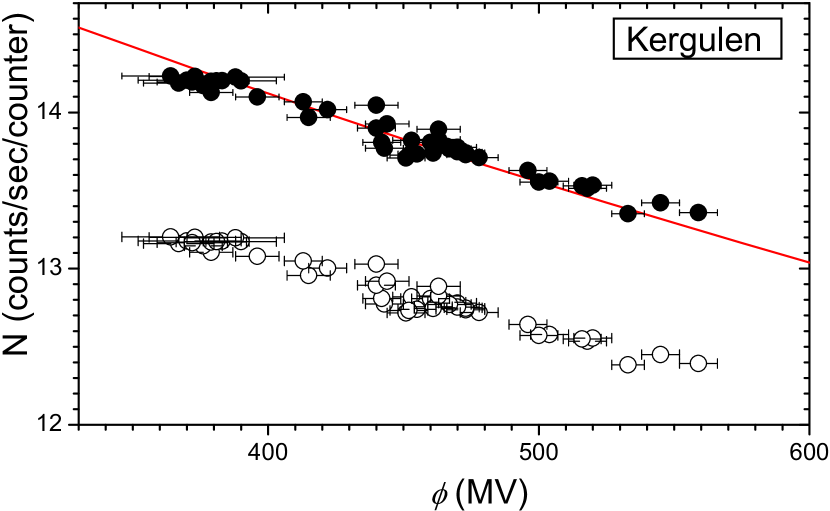
Figure 3: The mean count rate of the Kergulen NM during periods of PAMELA measurements (the corresponding values of $\phi$ are shown as the X-values) as recorded (open dots) and scaled using the best-fit factor $\kappa=1.078$. The red curve represents the model.

5 Reconstruction of the modulation potential

Once the scaling factor $\kappa$ is fixed for a given NM, the problem can be inverted so that from the measured (and corrected using the factor $\kappa$) count rate one can calculate the corresponding value of the modulation potential $\phi$. We did it by calculating the monthly values of $\phi$ for each NM listed in Table 1. The result is shown in Figure 4 with small dots. One can see that the spread of dots is very small during and around the calibration period in 2006–2010, but they diverge in the earlier part of the period, in the 1960–1970s.

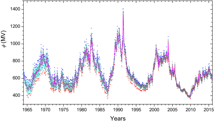
Figure 4: Reconstruction of the monthly modulation potential values (small dots) from individual NMs listed in Table 1. The red and blue dots correspond to Kiel and McMurdo NMs, respectively. The magenta line and the light blue shading represent the mean and the standard deviation of these individual reconstructions.

In the analysis, we considered also slow changes in the geomagnetic cutoff rigidity for each NM.

5.1 Long-term consistency of the NMs

Next, we check each of the analyzed NMs for long-term consistency. For that, we calculated the difference $\Delta\phi$ between the modulation potential calculated only from this NM data and that, calculated (as the mean and standard deviation) from the data of the other seven NMs in Table 1, excluding the tested one. This is shown in Figure 5.

We note that the Oulu NM (Fig. 5a) exhibits small ($\pm 25$ MV) deviations from the mean curve, but is always within the $1\sigma$ uncertainty of the latter, except for strong seasonal peaks in the earlier part. These peaks were caused by snow on the roof during winter months before 1974, when the Oulu NM was finally settled in a building with a pyramid-shaped warmed roof, so that snow was never accumulated above the NM since 1974. To avoid the uncontrolled effect of snow, we have excluded from further consideration the Oulu NM data for months January through March for years 1964–1973. The first months of data, in 1964, also depict a strong drift and were removed.

Inuvik, Moscow and Kergulen NMs (Fig. 5b–d) exhibit deviations up to $\pm 50$ MV from the mean curve, but are mostly within the $1\sigma$ uncertainty of the latter. Accordingly, data from these NMs were considered as they are.

The McMurdo NM (Fig. 5e) depicts a strong systematic deviation greatly exceeding $1\sigma$ limits, that was as much as about 100 MV before the 1980s. This is clearly seen in Fig. 4, where the blue dots lie systematically above the curve. This trend implies that the McMurdo NM tends to increase its count rate in time against other stations.

On the contrary, the Kiel NM (Fig. 5f) depicts an opposite but equally strong trend in the deviation, also exceeding systematically the $1\sigma$ limit. This is seen in Fig.4 as a systematic divergence of the red points. The systematic growth of $\Delta\phi$ implies that the Kiel NM count rate decreases in time against all other NMs. Interestingly, these two NMs nearly compensate each other in the composite, but grossly increase the error bars. Because of the systematic drifts, we do not include McMurdo and Kiel NMs into the final reconstruction of $\phi$.

The Apatity NM (Fig. 5g) depicts deviations within $\pm 50$ MV from the mean curve, mostly within the $1\sigma$ uncertainty of the latter. There is a spike in $\Delta\phi$ in 1969 (the first year of the NM operation). Because of it we only use the Apatity NM data after 1970. There is another spike in 1998–1999, but no correction was implied for this.

The Newark NM (Fig. 5g) depicts some deviations within $\pm 30$ MV from the mean curve, mostly always within the $1\sigma$ uncertainty of the latter. It also depicts a seasonal cycle, but it is small and not a subject to correction or removal.

Thus, from the eight preliminary selected NMs we use for further analysis six most stable ones (Oulu, Inuvik, Moscow, Kergulen, Apatity and Newark), while McMurdo and Kiel NMs depict systematic drifts and are not considered henceforth.

5.2 Extension before 1965

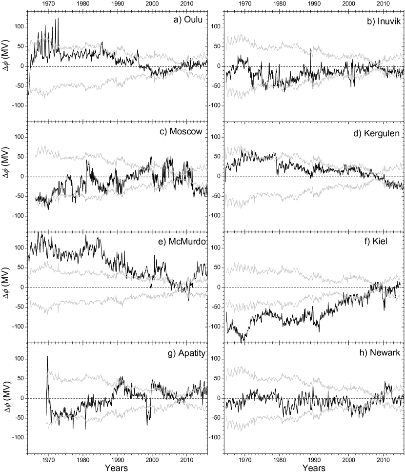
Figure 5: The difference $\Delta\phi$ between values of the modulation potential, computed from individual NMs (as indicated in the legends), and the mean $\phi$ computed using data from all the available NMs but this one. The grey lines bound the $\pm 1\sigma$ uncertainties of the mean series.

The consideration above was based on the World network of neutron monitors of the standard type NM64, which was introduced in 1964. Before that, there were several NMs of another design, called IGY (International Geophysical Year), the longest record being from the Climax NM (altitude $\approx 3400$ m, $P_{c}\approx$3 GV) from February 1951 until November 2006, and Mt.Washington ($\approx 1900$ m, $P_{c}\approx$ 1.3 GV) from November 1955 until June 1991. However, since they were not in operation during the PAMELA calibration period, their calibration was done via the overlap with the main world NM network since 1964. Because of their mid- and high-altitude location, the theoretical model (available for the sea level) is not applied. Accordingly, following the approach of Usoskin et al. (2011), for these two NMs we used an empirical relation between the NM count rate $N$ and the modulation potential $\phi$:

$$\phi={A\over N}+B,$$ (4)

where $A$ and $B$ are free parameters. Figure 6 shows a scatter plot of the monthly values of $\phi$ reconstructed from the Newark NM for the period 1965–2006 vs. the Climax NM’s inverted count rate. One can see that the relation (Eq. 4) is nearly perfectly linear and can be fitted (using the standard linear least-square method) with $A=(2.49\pm 0.02)\cdot 10^{5}$ MV/sec and $B=1597\pm 18$ MV. This Newark-vs-Climax relation can be used to estimate $\phi$ before 1965 from the Climax NM data. We constructed similar relations for all the six selected NMs, and thus have six series of $\phi$ for the period 1951–1964.

A similar analysis was performed also for the Mt.Washington NM data since 1955. As a result, for each month for the period 1955–1964 we have 12 values of $\phi$ (6 from Climax and 6 from Mt.Washington), from which we calculated the mean and the standard deviation as an assessment of the modulation potential for that period. For the period 1951–1955 only six $\phi$ series were used.

6 Results and discussions

6.1 Final series

The final reconstruction of the modulation potential is shown in Figure 7 along with its $1\sigma$ uncertainties, while digital values are given in Table 2.

The uncertainties are also shown separately in Figure 8. One can see that the uncertainty is small ($<10$ MV) during the PAMELA calibration period (denoted by the grey shading), moderate (20–25 MV) after the 1980’s and gradually increases back in time reaching $\approx 35$ MV around 1970, and stays at roughly this level before that. For the period 1955–1964, the spikes are caused by a discrepancy between Climax and Mt.Washington data. Before 1955, only the Climax NM data is available and the uncertainty is flat.

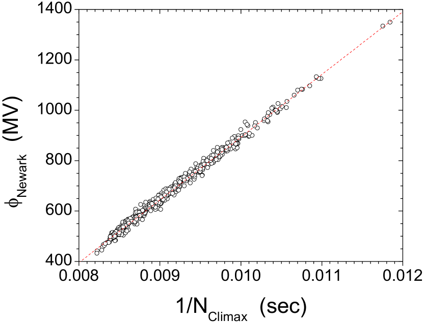
Figure 6: Scatter plot of monthly $\phi$ reconstructed from the Newark NM data for the period 1965–2000 and the inverted count rate of the Climax NM for the same period. The best-fit linear regression is shown by the red dotted line.

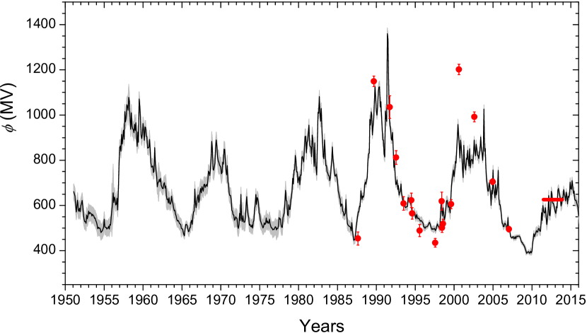
Figure 7: Monthly series of the modulation potential reconstructed here (black curve with grey shading depicting the $1\sigma$ uncertainties) along with the values of $\phi$ obtained by fitting balloon data. The data series is available in Table 2. The red stripe represents $\phi$ obtained from a fit to AMS-02 data.

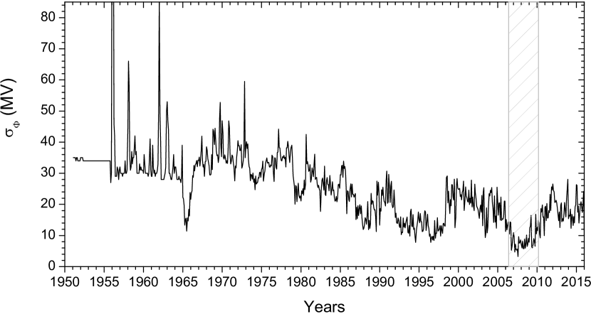
Figure 8: Standard error of the monthly modulation potential reconstruction (see Figure 4). The grey shaded region denotes the period of PAMELA calibration.

6.2 Comparison with other direct measurements

Beyond the PAMELA data, used for calibration of the NMs, we now compare the final modulation potential series with the values of $\phi$ obtained by fitting GCR spectra from short-time space- and balloon-borne measurements as shown in Figure 7. We used the following balloon- and space-borne data (see full details and data collection at http://tools.asdc.asi.it/cosmicRays.jsp?tabId=0) for the following measurements of the GCR energy spectrum: LEAP, MASS89, MASS91, IMAX92, POLAR, POLAR-2, BESS-TeV, BESS00, BESS93, BESS94, BESS95, BESS97, BESS98, BESS99, CAPRICE, CAPRICE98, AMS-01, AMS-02, with the original references to (Seo et al., 1991, 2001; Webber et al., 1991; Bellotti et al., 1999; Boezio et al., 1999, 2003; Alcaraz et al., 2000; Menn et al., 2000; Wang and Sheeley, 2002; Shikaze et al., 2007; Adriani et al., 2013; Aguilar et al., 2015; Abe et al., 2016)

One can see a general agreement between the overall curve and the individual points excepts for two balloon points, BESS00 and BESS-TeV, yielding too strong modulation in 2000 and 2002, respectively, and one point, BESS97, implying too low modulation in 1997. Note that disagreement of these data points with the NM data was mentioned also by Ghelfi et al. (2016).

However, such a comparison is not very representative, since the reconstructed series is with monthly resolution while individual flights had duration from several hours to several days, or, as in the case of AMS-02 data taking, several years. In Figure 9 we show a scatter plot of the Oulu NM count rates (scaled with the factor 1.121 – see Table 1, statistical errors are negligible) averaged over exactly the same periods as data taking for the balloon- and space-flight, vs. the fitted values of $\phi$ for these flights (as shown by red dots in Fig. 7). The solid black curve shows the model-predicted dependence between a polar NM count rate and the modulation potential. One can see that the agreement is quite good for the range of $\phi-$values covering PAMELA data used for calibration (red stars), viz. 300–700 MV. While PAMELA data lie tightly along the model curve, other data produce a large scatter, but still around the curve. On the other hand, data points lie slightly but systematically above the curve in the range of higher $\phi-$values 800–1200 MV. In particular, BESS00 and BESS-TeV, mentioned above, and MASS89 (used for calibration by Usoskin et al. (2011)) balloon data suggest a higher modulation than the model does, during periods of the active Sun. This may indicate that the model may slightly underestimate the modulation during such periods, but the lack of reliable data in this range (only 4–5 points vs. $\approx 60$ in the lower activity range) does not provide a solid ground for such a conclusion. The relations for other NMs (not shown) are similar to this example.

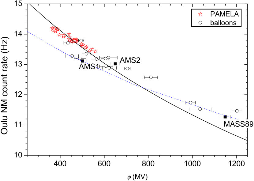
Figure 9: Comparison of this model (black solid curve) and experimental (points) count rates of the Oulu NM for the periods when measurements of the GCR spectra were available. Red stars – PAMELA periods used for calibration here; open circles – different balloon measurements; black squares – AMS-01 and MASS89, used for calibration in Usoskin et al. (2005) and Usoskin et al. (2011), as well as AMS-02. The dotted blue lines shows the model curve from Usoskin et al. (2011).

Thus, we conclude that the new reconstruction of the modulation potential is in good agreement with fragmentary direct measurements, at least for the periods of low and moderate solar activity.

6.3 Comparison with the previous reconstructions

We emphasize that the values of the modulation potential presented here, should not be directly compared with those published earlier. The reason is that the value of $\phi$ has no absolute physical meaning and depends on the LIS models used in its calculation (Usoskin et al., 2005; Herbst et al., 2010). It is only a useful parameter to describe the energy spectrum of GCR near Earth, with the fixed LIS value. Therefore, the fact that the values of $\phi$ presented here are different from the earlier ones does not imply different GCR spectra.

A scatter plot of the previously published modulation potential series (Usoskin et al., 2011) versus the results of this work is shown in Figure 10. The relation is very tight and slightly nonlinear.

The difference from the earlier models is caused by three main facts: (1) the use of the new NM yield function (Mishev et al., 2013, see also erratum therein); (2) the calibration of the NM responses directly to a large set of PAMELA data, while earlier models were linked to two points – AMS-01 and MASS89 (see Figure 9); and (3) the use of the updated LIS (Vos and Potgieter, 2015).

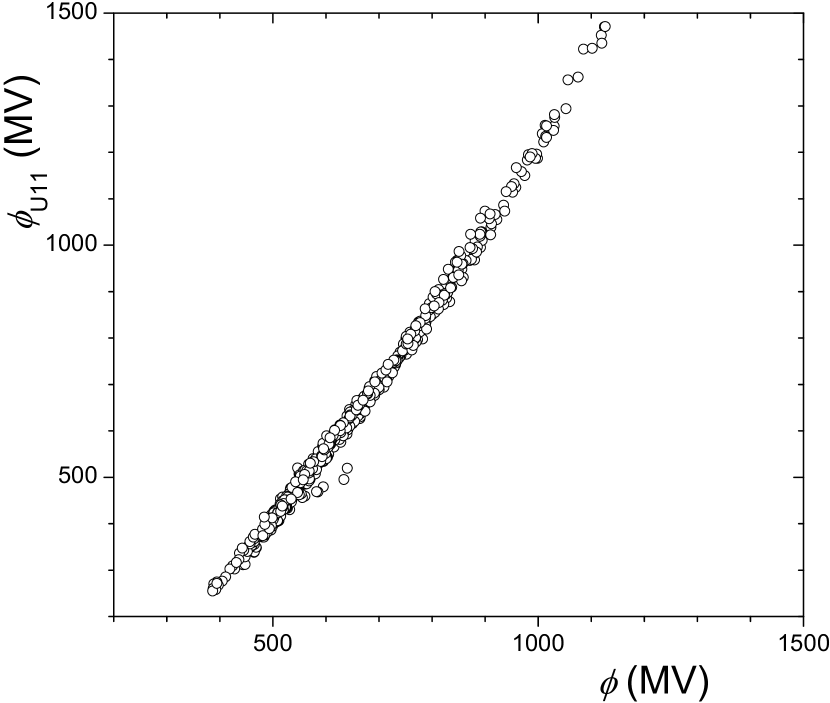
Figure 10: Comparison of monthly modulation potentials obtained here (X-axis) and those from (Usoskin et al., 2011) (Y-axis).

7 Conclusions

We have presented a new reconstruction of the heliospheric modulation potential for galactic cosmic rays during the neutron monitor era, since 1951. The new reconstruction is based on a new-generation specific yield function of a NM, exploits an updated model of the LIS, and applies a calibration to direct measurements of the GCR energy spectrum during 47 episodes by PAMELA space-borne spectrometer. The reconstruction is based on data from six standard NM64-type neutron monitors (Apatity, Inuvik, Kergulen, Moscow, Newark and Oulu) since 1965, and two IGY-type NMs (Climax and Mt.Washington) before that, all demonstrating stable operation over the decades. The new reconstruction is presented in Table 2.

We also tested the long-term stability of individual NMs and found that McMurdo and Kiel NMs exhibit essential drifts, while all other analyzed NMs are fairly stable on the multi-decadal time scale.

The presented series forms a benchmark record of the cosmic ray variability (in the NM energy range) for the last 60 years, and can be used to long-term studies in the fields of solar-terrestrial physics, atmospheric sciences, etc.

Table 2: Mean monthly value of the modulation potential (see Figure 7) for 1951–2016.

Yr/month	Jan	Feb	Mar	Apr	May	Jun	Jul	Aug	Sep	Oct	Nov	Dec
1951	N/A	661	651	642	601	571	600	623	580	574	588	573
1952	599	609	622	595	557	540	528	529	521	558	541	553
1953	575	563	569	565	564	553	561	556	553	543	545	533
1954	527	515	497	504	499	501	495	480	485	487	495	504
1955	539	505	503	503	496	500	500	508	496	516	513	549
1956	580	606	656	613	637	627	602	607	632	580	663	775
1957	856	863	840	914	872	902	933	893	1015	970	986	1046
1958	1040	1021	1078	1061	978	937	1010	954	939	936	922	959
1959	932	966	900	862	925	880	1071	1038	992	909	896	916
1960	962	932	888	947	945	906	905	854	856	856	892	850
1961	789	770	771	775	746	750	856	784	753	729	683	700
1962	704	715	705	720	689	682	675	675	696	701	677	686
1963	644	627	629	611	634	610	606	615	641	619	608	591
1964	577	579	562	553	538	531	534	529	521	518	516	499
1965	497	495	484	472	466	498	515	517	511	499	484	485
1966	501	503	525	534	517	551	571	575	673	614	591	616
1967	633	647	614	623	659	675	656	683	674	663	691	694
1968	680	688	693	684	708	752	746	732	758	801	883	854
1969	761	756	771	788	864	897	861	812	784	774	770	772
1970	768	740	746	791	783	849	848	801	754	736	776	704
1971	691	652	644	644	627	579	574	559	557	535	538	550
1972	545	542	509	499	516	565	533	649	542	529	554	532
1973	525	528	548	603	639	582	559	546	513	516	508	505
1974	514	500	527	535	580	603	648	605	635	629	614	566
1975	560	535	527	517	511	501	506	523	516	520	545	524
1976	531	521	522	540	520	508	501	500	492	495	494	499
1977	506	503	492	499	498	510	546	540	541	515	504	503
1978	547	560	568	613	667	623	619	560	555	603	583	583
1979	622	638	664	720	696	757	757	821	799	748	749	701
1980	717	727	692	735	734	813	817	803	793	853	905	906
1981	833	878	888	919	955	869	860	858	816	911	894	827
1982	773	877	784	765	735	880	1012	1008	1082	1008	973	1029
1983	936	876	816	807	890	834	776	777	748	743	733	731
1984	710	722	763	791	859	807	784	747	731	730	739	725
1985	709	665	654	637	629	596	606	606	575	571	554	561
1986	564	627	578	524	515	511	508	507	503	488	524	491
1987	466	446	447	451	470	507	527	551	571	571	597	594
1988	665	640	627	642	636	646	691	703	694	712	723	796
1989	828	832	980	956	1014	1000	912	952	986	1055	1126	1078
1990	1018	1000	1034	1103	1123	1125	1036	1059	999	941	890	889
1991	826	814	1018	990	972	1360	1334	1133	990	953	943	895
1992	889	923	852	769	797	734	693	696	713	671	688	646
1993	658	662	695	651	635	620	612	612	596	591	593	595
1994	596	635	625	631	612	610	594	574	556	564	563	570
1995	553	542	560	549	542	544	541	535	530	533	530	526
1996	522	505	505	499	505	505	506	509	514	522	525	517
1997	506	497	494	498	495	496	499	489	496	507	518	510
1998	505	500	498	559	606	583	554	589	558	536	552	576
1999	618	623	609	593	601	584	568	632	687	719	735	757
2000	728	759	795	788	846	899	958	908	868	811	889	859
2001	820	761	723	866	789	769	757	809	804	844	798	775
2002	851	767	798	804	801	785	830	889	841	820	870	849
2003	822	821	808	833	844	903	853	834	800	844	1026	840
2004	852	766	715	691	664	663	700	685	660	601	667	651
2005	757	675	656	634	692	647	663	686	755	629	603	603
2006	582	552	522	519	506	508	521	519	514	496	500	546
2007	492	498	484	463	459	456	459	463	453	455	462	453
2008	462	465	462	464	465	463	457	445	437	437	429	426
2009	421	414	407	398	389	393	393	396	389	390	397	390
2010	398	436	448	475	462	471	478	489	483	483	496	499
2011	488	486	513	568	534	599	576	568	568	590	549	516
2012	542	574	644	557	555	590	662	649	610	610	601	587
2013	571	565	595	590	667	675	656	644	630	598	610	635
2014	630	670	650	639	620	658	640	607	640	636	648	703
2015	674	672	709	684	654	664	628	622	623	612	603	590
2016	554	526	531	529	524	525	537	519	518	497	482	483