On the coupling time of the heat-bath process for the Fortuin-Kasteleyn random-cluster model

Abstract

We consider the coupling from the past implementation of the random-cluster heat-bath process, and study its random running time, or coupling time. We focus on hypercubic lattices embedded on tori, in dimensions one to three, with cluster fugacity at least one. We make a number of conjectures regarding the asymptotic behaviour of the coupling time, motivated by rigorous results in one dimension and Monte Carlo simulations in dimensions two and three. Amongst our findings, we observe that, for generic parameter values, the distribution of the appropriately standardized coupling time converges to a Gumbel distribution, and that the standard deviation of the coupling time is asymptotic to an explicit universal constant multiple of the relaxation time. Perhaps surprisingly, we observe these results to hold both off criticality, where the coupling time closely mimics the coupon collector’s problem, and also at the critical point, provided the cluster fugacity is below the value at which the transition becomes discontinuous. Finally, we consider analogous questions for the single-spin Ising heat-bath process.

1 Introduction

Since nontrivial models in statistical mechanics are rarely exactly solvable, Monte Carlo simulations provide an important tool for obtaining information on phase diagrams and critical exponents. The standard Markov-chain Monte Carlo procedure involves constructing a Markov chain with the desired stationary distribution, and then running the chain long enough that the resulting samples are close to stationarity. The central obstacle to practical applications of MCMC is that it is typically not known a priori how many steps are required in order to reach (approximate) stationarity. In principle, the answer to this question can be quantified by quantities such as the relaxation time or mixing time of the Markov chain (see below). However, rigorously proving practically useful upper bounds on such quantities is a very challenging task, as is their empirical estimation from simulations.

Coupling From The Past (CFTP), introduced by Propp and Wilson ProppWilson96 , is a refinement of the MCMC method, which automatically determines the required running time of the Markov chain, and then outputs exact samples, rather than approximate ones. The price that must be paid for these two significant benefits is that, unlike naive MCMC, the running time of CFTP is random. The key question in determining the efficiency of the CFTP method for a given application therefore becomes to understand the distribution of its random running time, or coupling time. The name “coupling from the past” derives from two key features of the method. Firstly, rather than running a single Markov chain, CFTP requires multiple Markov chains be run simultaneously (coupling). Secondly, the chains are not run forward from time 0, but are instead run from the past to time 0.

In this article, we present a detailed study of the coupling time for the heat-bath dynamics of the Fortuin-Kasteleyn (FK) random-cluster model. This process is one of the examples originally considered in ProppWilson96 , and has been the subject of several recent studies BlancaSinclair16 ; GuoJerrum16 ; ElciWeigel13 ; ElciWeigel14 ; DengGaroniSokal07_sweeny . As discussed in more detail below, when the cluster fugacity $q\geq 1$, this process possesses an important monotonicity property, which makes it an ideal candidate for an efficient implementation of CFTP.

We consider the FK process on $d$-dimensional tori, $\mathbb{Z}_{L}^{d}$, for $d=1,2,3$. Our methods are a combination of rigorous proof for $d=1$, and systematic Monte Carlo experiments for $d=2,3$. Based on our studies, we conjecture a number of results for the coupling time, which we state precisely in Section 2.4. Among them, we conjecture that, for generic choices of parameters $(p,q)$, the distribution of the coupling time (appropriately standardized) tends to a Gumbel distribution as $L\to\infty$. For the special case of $q=1$, the coupling time corresponds precisely to the coupon collector’s problem, for which the Gumbel limit is a classical result ErdosRenyi61 . The surprising observation is that such a limit appears not only to remain universally valid for the FK heat-bath process at any off-critical choice of $(p,q)\in(0,1)\times[1,\infty)$, but also at the critical point, provided $q$ is below the value at which the transition becomes discontinuous. In particular, we conjecture that this limit law holds for all $p\in(0,1)$ when $q\in[1,4)$ and $d=2$.

In addition, we find strong evidence that the standard deviation of the coupling time is asymptotic, as $L\to\infty$, to a universal constant times the relaxation time. Again, this is conjectured to hold not only off criticality for arbitrary $p\neq p_{\mathrm{c}}$ and $q\geq 1$, but also at $p=p_{\mathrm{c}}$, provided $q$ is below the value at which the transition becomes discontinuous. If true, this result suggests an efficient empirical method for estimating the relaxation time of the FK heat-bath process: simply generate a number of independent realizations of the coupling time and compute the sample variance. We emphasize that this result would imply that consideration of the coupling time can provide non-trivial information about the original Markov chain, and so its significance extends beyond possible applications of the CFTP method, to standard MCMC simulations of the FK heat-bath chain.

For comparison, we also briefly study the single-spin-update heat-bath process for the Ising model. Due to the slow mixing in the low temperature phase CesiGuadagniMartinelliSchonmann96 , our numerical results focus on the critical and high temperature regimes. In the high temperature regime, we find identical behaviour to that described above for the FK heat-bath process; in particular we find the same Gumbel limit law for the coupling time, and the same relationship between the relaxation time and the standard deviation of the coupling time. At criticality, however, the situation changes somewhat. The relaxation time and coupling time standard deviation do still appear to be asymptotically proportional, but now with a different proportionality constant. Moreover, while the standardized coupling time again appears to have a non-degenerate limit at criticality, the limit appears not to be of Gumbel type in this case.

1.1 Outline

Let us outline the remainder of this article. In Section 2 we define the FK heat-bath process, and discuss some relevant recent literature. We also define the coupling time, and explain its connection to CFTP. Section 2.4 summarizes our theorems and conjectures for the FK coupling time. Sections 3 and 4 respectively consider the moments and limiting distributions, and present numerical evidence to support the conjectures outlined in Section 2.4. Sections 5 and 6 provide proofs of Theorems 2.1 and 2.3, respectively. Section 7 summarizes the analogous results for the single-spin-update Ising heat-bath process. Finally, Appendix A establishes some relevant properties of autocorrelation functions of the FK heat-bath process, which we make use of in Section 3, and Appendix B discusses some technical lemmas concerning the coupon collector’s problem.

2 Fortuin-Kasteleyn heat-bath process

2.1 Definitions

The Fortuin-Kasteleyn random-cluster model is a correlated bond percolation model, which can be defined on an arbitrary finite graph $G=(V,E)$ with parameters $p\in[0,1]$ and $q>0$ via the measure

$$\phi(A)=\dfrac{1}{Z_{G}(p,q)}\,q^{k(A)}\,p^{|A|}\,(1-p)^{|A^{c}|},\qquad A\subseteq E$$ (2.1)

where $k(A)$ is the number of connected components (clusters) in the spanning subgraph $(V,A)$. The partition function, $Z_{G}(p,q)$ is closely related to the Tutte polynomial, and its computation is known to be a #P-hard problem Welsh93 ; JaegerVertiganWelsh90 . For $q=1$, the FK model coincides with standard bond percolation, while for integer $q>1$ it is intimately related to the $q$-state Potts model. Appropriate limits as $q\to 0$ also coincide with spanning forests and uniform spanning trees.

While our focus in the current article is on finite graphs, standard arguments (see e.g. Grimmett06 ) allow random-cluster measures to be defined on the infinite lattice $\mathbb{Z}^{d}$. In this setting, it is well known Grimmett06 that for given $q\geq 1$ and $d\geq 2$, there exists a critical probability $p_{\mathrm{c}}\in(0,1)$, such that the origin belongs to an infinite cluster with zero probability when $p<p_{\mathrm{c}}$, and with strictly positive probability when $p>p_{\mathrm{c}}$. The exact value of $p_{\mathrm{c}}$ when $d=2$ was recently proved BeffaraDuminilCopin12 to be $p_{\mathrm{c}}=\sqrt{q}/(1+\sqrt{q})$. The corresponding phase transition is said to be continuous if there is zero probability that the origin belongs to an infinite cluster at $p=p_{\mathrm{c}}$, and is discontinuous otherwise. It is known LaanaitMessagerMiracleSoleRuizShlosman91 that the transition is discontinuous for sufficiently large $q$. It is conjectured (Grimmett06, , Conjecture 6.32) that for every $d\geq 2$ there exists $q_{\ast}$ such that the transition is continuous for $q<q_{\ast}$ and discontinuous for $q>q_{\ast}$. This has recently been proved when $d=2$, and moreover the exact value $q_{\ast}=4$ was established, confirming a longstanding conjecture of Baxter Baxter78 . More precisely, in the specific case of $d=2$, the phase transition is continuous DuminilCopinSidoraviciusTassion15 for $1\leq q\leq 4$, and discontinuous DuminilCopinGagnebinHarelManolescuTassion16 for $q>4$. Although $p_{\mathrm{c}}=p_{\mathrm{c}}(q,d)$ depends on $d$ and $q$, and $q_{\ast}$ depends on $d$, for brevity, we shall not explicitly write this dependence when the values of $q,d$ are clear from the context.

To ease notation, for $A\subseteq E$ and $e\in E$, let $A_{e}:=A\setminus e$ and $A^{e}:=A\cup e$. Note that $A=A^{e}$ iff $e\in A$, and $A=A_{e}$ iff $e\not\in A$. An edge $e\in A$ is said to be occupied in $A$. An edge $e\in E$ is said to be pivotal to the configuration $A$ if $k(A_{e})\neq k(A^{e})$.

The FK heat-bath process has transition matrix $P=\dfrac{1}{m}\sum_{e\in E}P_{e}$ where

$$\begin{split}P_{e}(A,B)&:=\begin{cases}p(A,e),&B=A^{e},\\ 1-p(A,e),&B=A_{e},\\ 0,&\text{otherwise},\end{cases}\\ p(A,e)&:=\frac{\phi(A^{e})}{\phi(A^{e})+\phi(A_{e})}=\begin{cases}\tilde{p},&e\text{ is pivotal to }A,\\ p,&\text{otherwise},\end{cases}\\ \tilde{p}&:=\dfrac{p}{1+(q-1)(1-p)}.\end{split}$$ (2.2)

Note that, if $q\geq 1$ and ${p\in(0,1)}$, we have $\tilde{p}\leq p$, with equality iff $q=1$.

We now proceed to define the central quantity of interest in this article, the coupling time of the FK heat-bath process. It should be emphasized that the coupling time, and the corresponding CFTP algorithm, are not uniquely determined by the transition probabilities of the process, but rather by the particular random mapping representation that is chosen. Random mapping representations for Markov chains provide convenient methods for constructing useful couplings, and also for constructing practical computational implementations LevinPeresWilmer09 .

We focus attention on the following random mapping representation for $P$. Define $f:2^{E}\times E\times[0,1]\to 2^{E}$ via

$$f(A,e,u):=\begin{cases}A^{e},&u\leq p(A,e),\\ A_{e},&u>p(A,e).\end{cases}$$ (2.3)

Let $\mathcal{E}$ and $U$ be independent, with $\mathcal{E}$ uniform on $E$ and $U$ uniform on $[0,1]$. By construction, $\mathbb{P}(f(A,\mathcal{E},U)=B)=P(A,B)$, and so $(f,\mathcal{E},U)$ defines a random mapping representation for $P$ LevinPeresWilmer09 . It is straightforward to verify that $f$ is monotonic: for any fixed $e\in E$ and $u\in[0,1]$, if $A\subseteq B$, then $f(A,e,u)\subseteq f(B,e,u)$. This random mapping representation corresponds precisely to the manner in which a computational physicist would implement the transition matrix $P$ in practice.

Let $(\mathcal{E}_{t},U_{t})_{t\in\mathbb{N}^{+}}$ be an iid sequence of copies of $(\mathcal{E},U)$. Define $\mathcal{T}_{t}$ by $\mathcal{T}_{0}=E$ and $\mathcal{T}_{t+1}=f(\mathcal{T}_{t},\mathcal{E}_{t+1},U_{t+1})$. We refer to $\mathcal{T}_{t}$ as the top chain. Likewise, the bottom chain is defined by $\mathcal{B}_{0}=\emptyset$ and $\mathcal{B}_{t+1}=f(\mathcal{B}_{t},\mathcal{E}_{t+1},U_{t+1})$. By construction, both $(\mathcal{T}_{t})_{t\in\mathbb{N}}$ and $(\mathcal{B}_{t})_{t\in\mathbb{N}}$ are Markov chains with transition matrix $P$. The coupled process $(\mathcal{B}_{t},\mathcal{F}_{t})_{t\in\mathbb{N}}$ is the fundamental object of consideration in this article. For brevity, in what follows, we will refer to the coupled process $(\mathcal{B}_{t},\mathcal{F}_{t})_{t\in\mathbb{N}}$ as “the FK heat-bath coupling”.

We define the coupling time of the FK heat-bath process to be

$$T:=\min\{t\in\mathbb{N}:\mathcal{T}_{t}=\mathcal{B}_{t}\}.$$ (2.4)

Note that, strictly speaking, the coupling time is a property of the FK heat-bath coupling, rather than of a single FK heat-bath process. Also note that, by monotonicity, a Markov chain started at time 0 in any state $A\subseteq E$ will have coalesced with $\mathcal{T}_{t}$ and $\mathcal{B}_{t}$ by time $t=T$, so $\mathcal{T}_{T}$ can be viewed as the state of the Markov chain at the first time in which the initial state has been forgotten by the above coupling. As discussed further in Section 2.3, the coupling time has the same distribution as the running time of the CFTP algorithm.

2.2 Previous studies of FK Glauber processes

A reversible Markov chain with stationary distribution (2.1), which is local in the sense that at most one edge is updated per time step, is typically referred to as a Glauber process for the FK model. The two most commonly studied Glauber processes for the FK model are the heat-bath process, as studied here, and the Metropolis process, as first studied numerically in Sweeny83 .

As a consequence of general results concerning heat-bath chains DyerGreenhillUllrich14 , the transition matrix of the FK heat-bath process, $P$, has non-negative eigenvalues. If $\lambda_{2}$ denotes the second-largest eigenvalue of $P$, the relaxation time LevinPeresWilmer09 of $P$ is

$$t_{\mathrm{rel}}:=\frac{1}{1-\lambda_{2}}.$$ (2.5)

A closely related quantity is the exponential autocorrelation time MadrasSlade96 ; Sokal97 , defined by

$$t_{\exp}:=\frac{-1}{\ln(\lambda_{2})}=\frac{-1}{\ln(1-1/t_{\mathrm{rel}})}.$$ (2.6)

It is easily verified that

$$t_{\mathrm{rel}}-1\leq t_{\exp}\leq t_{\mathrm{rel}}.$$ (2.7)

Another quantity of importance is the mixing time LevinPeresWilmer09 , defined by

$$t_{\mathrm{mix}}(\epsilon):=\max_{A\subseteq E}\,\min_{t\in\mathbb{N}}\,\{\|P^{t}(A,\cdot)-\phi\|_{\mathrm{TV}}\leq\epsilon\},$$ (2.8)

where $\|\cdot\|_{\mathrm{TV}}$ denotes total variation distance. Since $t_{\mathrm{mix}}(\epsilon)\leq\lceil\log_{2}\epsilon^{-1}\rceil\,t_{\mathrm{mix}}(1/4)$, one also defines $t_{\mathrm{mix}}:=t_{\mathrm{mix}}(1/4)$ LevinPeresWilmer09 . Combining (LevinPeresWilmer09, , Theorem 12.3) and (LevinPeresWilmer09, , Theorem 12.4) with Lemma 5.1 implies that for the FK heat-bath process

$$\frac{t_{\mathrm{rel}}-1}{2}\leq t_{\mathrm{mix}}\leq\ln\left(\frac{4q^{2}}{p(1-p)}\right)\,m\,t_{\mathrm{rel}}.$$ (2.9)

The quantities $t_{\mathrm{rel}}$, $t_{\exp}$ and $t_{\mathrm{mix}}$ all quantify the rate at which a Markov chain approaches stationarity, of mixes LevinPeresWilmer09 .

Numerical studies Gliozzi02 ; WangKozanSwendsen02 ; DengGaroniSokal07_sweeny of FK Glauber processes suggest that their mixing in the neighbourhood of continuous phase transitions can be surprisingly efficient; comparable to, and possibly faster than, non-local cluster algorithms such as the Swendsen-Wang and Chayes-Machta processes SwendsenWang87 ; ChayesMachta98 . In addition, it was observed numerically in DengGaroniSokal07_sweeny that, for the FK Metropolis-Glauber process at criticality on the square and simple-cubic lattices, certain observables apparently decorrelate asymptotically faster than a single sweep (i.e. in time $o(|E|)$), suggesting FK Glauber processes could have significant advantages over cluster algorithms.

Significant progress has recently been made in rigorously bounding the mixing time of FK Glauber processes. In GuoJerrum16 , the mixing time of the $q=2$ FK Metropolis-Glauber process on a graph with $m$ edges and $n$ vertices was shown to be $O(n^{4}m^{3})$. In addition, precise asymptotics were given in BlancaSinclair16 for the case of $q\geq 1$ on $L\times L$ boxes in $\mathbb{Z}^{2}$, showing that $t_{\mathrm{mix}}\asymp L^{2}\ln L$, provided $p\neq p_{\mathrm{c}}$. Even more recently, it has been shown in GheissariLubetzky16 that $t_{\mathrm{mix}}=O(L^{\ln L})$ on two-dimensional tori $\mathbb{Z}_{L}^{2}$ at $p=p_{\mathrm{c}}$.

An important practical issue when simulating FK Glauber processes is the need to identify whether the edge to be updated is pivotal to the current edge configuration. Sweeny Sweeny83 proposed an algorithm for performing the necessary connectivity checks, which was applicable to planar graphs. In Elci15_thesis ; ElciWeigel13 ; ElciWeigel14 , it was demonstrated that this algorithmic problem can be efficiently solved by utilizing, and adapting, dynamic connectivity algorithms and appropriate data structures introduced in HolmDeLichtenbergThorup01 . These latter methods are applicable to arbitrary graphs, and can perform the required pivotality tests in time which is poly-logarithmic in the graph size.

2.3 Coupling from the past

For completeness, in this section we present a brief review of the CFTP method applied to the FK heat-bath process. We note however that the material in this section, which follows the discussion in ProppWilson96 , serves only as motivation for studying the coupling time (2.4), and none of the concepts introduced in this section will be required outside of this section.

Let $(\mathcal{E}_{t},U_{t})_{t\geq 0}$ be an iid sequence of copies of $(\mathcal{E},U)$, define random maps $f_{-t}:=f(\cdot,\mathcal{E}_{t},U_{t})$, and for $t\in\mathbb{N}^{+}$ form the compositions

$$F_{-t}^{0}:=f_{0}\circ f_{-1}\circ\ldots\circ f_{-(t-1)}.$$ (2.10)

We can then define the backward coupling time to be

$$\mathfrak{T}:=\min\{t\in\mathbb{N}^{+}:F_{-t}^{0}(E)=F_{-t}^{0}(\emptyset)\}.$$ (2.11)

As first shown in ProppWilson96 , the random state $F_{-\mathfrak{T}}^{0}(E)=F_{-\mathfrak{T}}^{0}(\emptyset)$ is an exact sample from the FK distribution (2.1). Algorithmically, a single step of the above procedure corresponds to starting chains in states $E$ and $\emptyset$ at some point in the past, and running them until time 0. This procedure is then applied iteratively, starting the chains at ever more distant times in the past, and terminating the iteration at the first time that the chains started at $E$ and $\emptyset$ agree at time 0.

To appreciate why the resulting state $F_{-\mathfrak{T}}^{0}(E)$ is distributed according to (2.1), we can make the following observations. Firstly, by monotonicity, if $F_{-t}^{0}(E)=F_{-t}^{0}(\emptyset)$ then $F_{-t}^{0}(A)=F_{-t}^{0}(E)$ for every $A\subseteq E$. Secondly, if $F_{-t}^{0}(E)=F_{-t}^{0}(\emptyset)$ then $F_{-s}^{0}(E)=F_{-s}^{0}(\emptyset)$ for every $s\geq t$. Therefore, the state $F_{-\mathfrak{T}}^{0}(E)$ coincides with $F_{-s}^{0}(A)$ for any $s\geq\mathfrak{T}$ and $A\subseteq E$. In this sense, we can picture $F_{-\mathfrak{T}}^{0}(E)$ as the state, at time $t=0$, of a Markov chain that started at an arbitrary state in the infinite past.

For comparison, note that performing a standard Markov-chain Monte Carlo simulation simply corresponds to composing the sequence of random maps in the opposite order to (2.10). Specifically, to defining random maps $f_{t}:=f(\cdot,\mathcal{E}_{t},U_{t})$ and forming the compositions

$$F_{0}^{t}:=f_{t}\circ\ldots\circ f_{1}.$$

Even though, by monotonicity, we have $F_{0}^{T}(E)=F_{0}^{T}(A)=F_{0}^{T}(\emptyset)$ for all $A\subseteq E$, there is no reason to suspect $F_{0}^{T}(E)$ should have distribution (2.1).

Despite the significant differences between the forward and backward couplings, it can be shown, quite generally, that forward and backward coupling times are identically distributed ProppWilson96 . As a consequence, to study the behaviour of the random running time $\mathfrak{T}$ of CFTP, it suffices to consider only the forward coupling time $T$, defined in (2.4).

The CFTP algorithm described above is the simplest version, however a number of algorithmic improvements have been devised. In particular, rather than choosing the restart times to be $-1,-2,-3,\ldots$, the restart times can be chosen to be $-a_{1},-a_{2},\ldots$ for any monotonic natural sequence $a_{1},a_{2},\ldots$. See the pedagogical discussions in Jerrum98 ; Haggstrom03 ; LevinPeresWilmer09 for more details on CFTP algorithms.

2.4 Behaviour of the coupling time

We now summarize our main results for the coupling time. We begin with some general results, holding on arbitrary finite connected graphs, which relate the coupling time (2.4) to $t_{\mathrm{mix}}$ and $t_{\exp}$. Theorem 2.1 is a slight refinement, in the specific setting of the FK heat-bath coupling, of the results presented in (ProppWilson96, , Section 5). Its proof is deferred until Section 5.

Theorem 2.1.

Consider the FK heat-bath coupling with parameters $p\in(0,1)$ and $q\geq 1$, on a finite connected graph with $m\geq 1$ edges, and let $\psi:=\psi(p,q):=\dfrac{q^{2}}{p(1-p)}$. Then

$$\frac{e^{-t/t_{\exp}}}{2}\leq\mathbb{P}(T>t) \leq e^{(\ln(\psi)+2)\,m-t/t_{\exp}},$$ (2.12)

$$\frac{t_{\mathrm{mix}}-1}{4}\leq\mathbb{E}(T) \leq\min\left\{12\,\log_{2}(4m)\,t_{\mathrm{mix}},\,4(\log_{2}(\psi)+3)\,m\,t_{\exp}\right\},$$ (2.13)

$$\sqrt{\operatorname{var}(T)} \leq\min\left\{15\,\log_{2}(4m)\,t_{\mathrm{mix}},\,5(\log_{2}(\psi)+3)\,m\,t_{\exp}\right\}$$ (2.14)

Remark 2.2.

In the special case of $L\times L$ boxes in $\mathbb{Z}^{2}$, with $p\neq p_{\mathrm{c}}$, we can combine the mixing time bound presented in BlancaSinclair16 with Theorem 2.1 to conclude that both $\mathbb{E}(T)$ and $\sqrt{\operatorname{var}(T)}$ are $O(L^{2}\,\ln^{2}L)$, and that $\mathbb{E}(T)$ is $\Omega(L^{2}\ln L)$. Likewise, the results in GheissariLubetzky16 imply that, at $p=p_{\mathrm{c}}$, both $\mathbb{E}(T)$ and $\operatorname{var}(T)$ are $L^{O(\ln L)}$ on $\mathbb{Z}_{L}^{2}$.

As mentioned briefly in Section 1, the coupling time is related to the coupon collector’s problem. We now make this connection more precise. Consider a finite connected graph $G=(V,E)$ with $|E|=m$ and let

$$W:=\min\{t\in\mathbb{N}^{+}:\{\mathcal{E}_{1},\ldots,\mathcal{E}_{t}\}=E\}.$$ (2.15)

The random variable $W$ is the coupon collector’s time, for the edge process $(\mathcal{E}_{t})_{t\in\mathbb{N}^{+}}$, and its behaviour is well-understood ErdosRenyi61 ; LevinPeresWilmer09 . It is elementary to show (see e.g. Posfai10 ) that

$$\mathbb{E}(W) =m\,H_{m}\,\sim m\ln(m),$$ (2.16)

$$\operatorname{var}(W) =m^{2}H_{m}^{(2)}-m\,H_{m}\sim\frac{\pi^{2}}{6}m^{2},$$ (2.17)

as $m\to\infty$, where $H_{m}^{(k)}:=\sum_{i=1}^{m}i^{-k}$ is the generalized Harmonic number GrahamKnuthPatashnik94 of order $k$, and $H_{m}:=H_{m}^{(1)}$. Moreover, as first shown in ErdosRenyi61 , for any $x\in\mathbb{R}$ we have

$$\lim_{m\to\infty}\mathbb{P}[W\leq\mathbb{E}(W)+x\sqrt{\operatorname{var}(W)}]=G(x),$$ (2.18)

where

$$G(x):=\exp\left(-\exp\left(-\dfrac{\pi}{\sqrt{6}}\,x-\gamma\right)\right),\quad x\in\mathbb{R},$$ (2.19)

is the distribution function of the Gumbel distribution with zero mean and unit variance, and $\gamma$ is the Euler-Mascheroni constant.

Since the top and bottom chains cannot coalesce until every edge has been updated at least once, we clearly have

$$T\geq W.$$ (2.20)

Moreover, if $t\in\mathbb{N}^{+}$, then by monotonicity, $\mathcal{B}_{t}$ and $\mathcal{T}_{t}$ will disagree on the edge $\mathcal{E}_{t}$ iff $\mathcal{E}_{t}\in\mathcal{T}_{t}$ and $\mathcal{E}_{t}\not\in\mathcal{B}_{t}$. In turn, this will occur iff: $\mathcal{E}_{t}$ is pivotal to $\mathcal{B}_{t-1}$ but not pivotal to $\mathcal{T}_{t-1}$; and $\tilde{p}<U_{t}\leq p$. If $G$ is a tree, every edge is pivotal to every $A\subseteq E$, and the first condition cannot occur. If $q=1$, then $\tilde{p}=p$ and the second condition cannot occur. It follows that if $q=1$, or if $G$ is a tree, then $T=W$ identically.

Our main interest in this article is the case that $G$ is $\mathbb{Z}_{L}^{d}$ for some choice of $L$ and $d$. In this case, $T$ is certainly not identically equal to $W$. For $d=1$ however, Theorem 2.3 shows that, for large $L$, the behaviour of $T$ closely mimics that of $W$. To emphasize the dependence of $T$ and $W$ on $L$ we append subscripts in the remainder of this section.

Theorem 2.3.

Consider the FK heat-bath coupling on $\mathbb{Z}_{L}$ with parameters $p\in(0,1)$ and $q\geq 1$. Then, as $L\to\infty$, we have:

1. $\mathbb{E}(T_{L})\sim\mathbb{E}(W_{L})$.

2. $\operatorname{var}(T_{L})\sim\operatorname{var}(W_{L})$

3. $\mathbb{P}[T_{L}\leq\mathbb{E}(T_{L})+x\sqrt{\operatorname{var}(T_{L})}]\to G(x)$ for each $x\in\mathbb{R}$.

4. $t_{\mathrm{rel}}\asymp L$.

Intuitively, one expects the behaviour of the model on $\mathbb{Z}_{L}$ to be representative of the sub-critical behaviour on $\mathbb{Z}_{L}^{d}$ for any $d\geq 1$. This suggests that the sub-critical behaviour on $\mathbb{Z}_{L}^{d}$ should again be governed by the coupon collector time. Conjectures 2.4 and 2.5 formalize this intuition in the case of the mean and variance. These conjectures are consistent with the rigorous bounds known in two dimensions, discussed in Remark 2.2.

To ease notation in what follows, we define $\mu_{T}(L):=\mathbb{E}(T_{L})$ and $\sigma_{T}(L):=\sqrt{\operatorname{var}(T_{L})}$, and likewise set $\mu_{W}(L):=\mathbb{E}(W_{L})$ and $\sigma_{W}(L):=\sqrt{\operatorname{var}(W_{L})}$. For brevity, we omit explicit mention of the dependence of $\mu_{T}$ and $\sigma_{T}$ on $p,q$. In later sections, we shall also often omit explicit mention of their $L$ dependence.

Conjecture 2.4 (Off-critical mean).

Consider the FK heat-bath coupling on $\mathbb{Z}_{L}^{d}$ with $d\geq 2$, $q\geq 1$ and $p\in(0,1)$ such that $p\neq p_{\mathrm{c}}$. There exists $C(p,q,d)\geq 1$ such that as $L\to\infty$

$$\mu_{T}(L)\sim C(p,q,d)\,\mu_{W}(L).$$

Numerical evidence in support of Conjecture 2.4 is presented in Section 3.1.

We note that, if correct, Conjecture 2.4 combined with (2.16) and the recent mixing time bound BlancaSinclair16 implies that for $d=2$ we have $\mu_{T}(L)\asymp t_{\mathrm{mix}}(L)$ whenever $p\neq p_{\mathrm{c}}$. It seems natural to expect that this in fact holds in all dimensions. Given the difficulty of estimating $t_{\mathrm{mix}}$ numerically, however, we have no empirical evidence to directly support the claim $\mu_{T}(L)\asymp t_{\mathrm{mix}}(L)$, and we therefore do not state it formally as a conjecture.

Conjecture 2.5 (Off-critical variance).

Consider the FK heat-bath coupling on $\mathbb{Z}_{L}^{d}$ with $d\geq 2$, $q\geq 1$ and $p\in(0,1)$ such that $p\neq p_{\mathrm{c}}$. There exists $C(p,q,d)\geq 1$ such that as $L\to\infty$

$$\sigma_{T}(L)\sim C(p,q,d)\,\sigma_{W}(L).$$

Numerical evidence in support of Conjecture 2.5 is presented in Section 3.1.

One consequence of Theorem 2.3 is that $\sigma_{T}(L)\asymp t_{\mathrm{rel}}(L)$ when $d=1$. While no precise asymptotics appear to be known for $t_{\mathrm{rel}}$ when $d>1$, from a physical standpoint one expects that $t_{\mathrm{rel}}(L)\asymp L^{d}$ for $p\neq p_{\mathrm{c}}$, in any dimension $d$. Under this additional hypothesis, Conjecture 2.5 is equivalent to the conjecture that $\sigma_{T}(L)\asymp t_{\mathrm{rel}}(L)$. We shall return to this observation shortly.

Combining Conjectures 2.4 and 2.5 with (2.16) and (2.17) implies $\sigma_{T}(L)/\mu_{T}(L)$ goes to zero as $L\to\infty$. It then follows from Chebyshev’s inequality that for any $\epsilon>0$

$$\mathbb{P}[(1-\epsilon)\mu_{T}(L)<T_{L}<(1+\epsilon)\mu_{T}(L)]\geq 1-o(1),\qquad L\to\infty.$$

While the moments of $T_{L}$ do not behave like the corresponding moments of $W_{L}$ at $p_{\mathrm{c}}$, our numerical results do suggest that $\mu_{T}(L)$ remains the dominant time scale at criticality when $q<q_{\ast}$.

Conjecture 2.6.

Consider the FK heat-bath coupling on $\mathbb{Z}_{L}^{d}$ with $d\geq 2$, $q\geq 1$ and $p\in(0,1)$ such that if $q\geq q_{\ast}$ then $p\neq p_{\mathrm{c}}$. Then $\sigma_{T}(L)/\mu_{T}(L)\to 0$ as $L\to\infty$.

Numerical evidence in support of Conjecture 2.6 is presented in Section 3.2. Our numerical results suggest that Conjecture 2.6 does not hold at $p=p_{\mathrm{c}}$ when $q\geq q_{\ast}$.

In light of Conjectures 2.4 and 2.5, one is tempted to conjecture further that Part (iii) of Theorem 2.3, the Gumbel limit law, also extends to the case $d>1$ in the off-critical regime. Section 4.1 provides strong numerical evidence to support this claim. What is perhaps more surprising, however, is that the numerical results of Section 4.2 strongly suggest that the Gumbel limit law holds even at the critical point, provided $q<q_{\ast}$. This is despite the fact that $\mu_{T}(L)$ and $\sigma_{T}(L)$ certainly do not behave like the analogous moments of $W_{L}$ at $p=p_{\mathrm{c}}$. In this sense, it seems $T_{L}$ displays a “superuniversal” central limit theorem, independent of $q$, for all $q<q_{\ast}$. Conjecture 2.7 formalizes this claim.

Conjecture 2.7 (Limiting Distribution).

Consider the FK heat-bath coupling on $\mathbb{Z}_{L}^{d}$ with $d\geq 2$, $q\geq 1$ and $p\in(0,1)$ such that if $q\geq q_{\ast}$ then $p\neq p_{\mathrm{c}}$. Then

$$\lim_{L\rightarrow\infty}\mathbb{P}[T_{L}\leq\mu_{T}(L)+x\sigma_{T}(L)]=G(x),\qquad\text{ for each }x\in\mathbb{R}.$$

Numerical evidence in support of Conjecture 2.7 is presented in Section 4. Our numerical results suggest the Gumbel limit law does not hold at $p=p_{\mathrm{c}}$ when $q>q_{\ast}$. The special case $(p,q)=(p_{\mathrm{c}},q_{\ast})$ appears to be rather subtle, and we are hesitant to make any predictions concerning it.

If we assume that Conjecture 2.7 is correct, then combining it with Theorem 2.1 suggests that $\sigma_{T}(L)$ is asymptotic to $t_{\exp}(L)$ as $L\to\infty$. Indeed, setting $t=\mu_{L}+x\,\sigma_{L}$ in (2.12) implies

$$-\ln(2)-\frac{\mu_{T}}{t_{\exp}}-\frac{\sigma_{T}}{t_{\exp}}\,x\leq\ln\mathbb{P}(T_{L}>\mu_{T}+x\,\sigma_{T})\leq d(\ln(\psi)+2)\,L^{d}-\frac{\mu_{T}}{t_{\exp}}-\frac{\sigma_{T}}{t_{\exp}}\,x.$$

However, it is easily obtained from (2.19) that

$$\ln[1-G(x)]\sim-\gamma-\frac{\pi}{\sqrt{6}}\,x,\qquad x\to\infty.$$

Combining these facts with Conjecture 2.7 then motivates the following conjecture.

Conjecture 2.8 (Variance).

Consider the FK heat-bath coupling on $\mathbb{Z}_{L}^{d}$ with $d\geq 2$, $q\geq 1$ and $p\in(0,1)$ such that if $q\geq q_{\ast}$ then $p\neq p_{\mathrm{c}}$. Then

$$\sigma_{T}(L)\sim\frac{\pi}{\sqrt{6}}t_{\exp}(L),\qquad L\to\infty.$$

Numerical evidence in support of Conjecture 2.8 is presented in Section 3.3.

Remark 2.9.

Recall that a sequence of chains has a cutoff LevinPeresWilmer09 if, for all $\epsilon>0$, we have $t_{\mathrm{mix}}(L,\epsilon)/t_{\mathrm{mix}}(L,1-\epsilon)\to 1$ as $L\to\infty$. A necessary condition (LevinPeresWilmer09, , Proposition 18.4) for cut-off is that $t_{\mathrm{mix}}(L)/t_{\mathrm{rel}}(L)\to\infty$ as $L\to\infty$. If one assumes the validity of Conjectures 2.6 and 2.8, and also assumes that $t_{\mathrm{mix}}\asymp\mu_{T}(L)$, then this necessary condition will be satisfied for the FK heat-bath process on $\mathbb{Z}_{L}^{d}$ with $d\geq 1$, $q\geq 1$ and any $p\in(0,1)$ such that if $q\geq q_{\ast}$ then $p\neq p_{\mathrm{c}}$. It is therefore tempting to speculate that the FK heat-bath process exhibits cutoff for all such parameter choices.

For comparison, in Section 7 we consider analogous questions for the single-spin Ising heat-bath process. Above the critical temperature, our results suggest the behaviour is identical to that conjectured above for the FK heat-bath process. Specifically, the mean and variance of the coupling time are asymptotic to a constant $C\geq 1$ multiple of their coupon collector analogues, the standard deviation is asymptotic to $(\pi/\sqrt{6})\,t_{\exp}$, and the standardized quantity $(T-\mu_{T})/\sigma_{T}$ has limiting distribution $G(x)$. At the critical temperature, however, the behaviour is somewhat different. In that case, our evidence suggests $\sigma_{T}/\mu_{T}$ tends to a positive constant, rather than zero. Moreover, while we do still observe that $(T-\mu_{T})/\sigma_{T}$ has a non-degenerate limiting distribution, this distribution does not appear to be $G(x)$. We have not attempted to identify the form of the limiting distribution in this case. Finally, we again find strong evidence that $\sigma_{T}\sim C\,t_{\exp}$, but now with $C\neq\pi/\sqrt{6}$. We state our conjectured behaviour for the Ising heat-bath process more formally in Conjecture 7.1, in Section 7.2.

The observation that $\sigma_{T}/\mu_{T}$ tends to zero for the critical FK heat-bath process, but not the critical Ising heat-bath process, provides another perspective on the improved efficiency of the former compared with the latter, over and above the empirical observation of critical speeding-up and smaller relaxation time DengGaroniSokal07_sweeny . Moreover, if one postulates (admittedly, in the absence of any significant evidence) that $\mu_{T}\asymp t_{\mathrm{mix}}$, and assumes the validity of Conjecture 2.8 and its analogue for the Ising heat-bath process, then one concludes that $t_{\mathrm{mix}}/t_{\mathrm{rel}}$ diverges for the critical FK heat-bath process, but not for the critical Ising heat-bath process. As noted in Remark 2.9, this would immediately rule out cutoff in the Ising heat-bath process, but still allow for its existence in the FK heat-bath process.

3 Moments

We now present numerical evidence in support of Conjectures 2.4, 2.5, 2.6 and 2.8. As discussed in Section 2.1, for $d=2$ the exact value of $p_{\mathrm{c}}(q)$ is known, and it is known that $q_{\ast}=4$. Neither $p_{\mathrm{c}}(q)$ nor $q_{\ast}$ are known when $d=3$. However, numerical studies DengGaroniSokalZhou ; Hartmann05 ; Gliozzi02 of the case $q=2.2$ have provided convincing evidence that the transition at $q=2.2$ is continuous, suggesting $q_{\ast}>2.2$. In our simulations for $d=3$ we relied on the following estimated critical points: $p_{\mathrm{c}}(1.5)=0.31157497$, $p_{\mathrm{c}}(1.8)=0.34096070$, $p_{\mathrm{c}}(2)=0.35809124$ and $p_{\mathrm{c}}(2.2)=0.37361401$. The values for $q=1.5,1.8,2.2$ are taken from DengGaroniSokalZhou , while the value for $q=2$ is taken from DengBlote03 .

3.1 Off criticality

We begin by considering the off-critical mean. In order to test Conjecture 2.4, Fig. 1(a) plots Monte Carlo estimates of $\mu_{T}$, scaled by the exact form of $\mu_{W}$ from (2.16), on a linear-log scale, for $d=2,3$, with a variety of $q$ values, and off-critical $p$ values. The agreement is excellent. The data are clearly converging to a constant $C(p,q,d)\geq 1$. The solid black line in Fig. 1(a) corresponds to the case $q=1$, for which $C(p,q,d)=1$ identically. It is conceivable, from the data at hand, that $C(p,q,d)=1$ for all off-critical parameter choices $(p,q,d)$, however the current evidence does not seem strong enough for us to actually conjecture that this is the case.

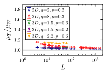
(a)

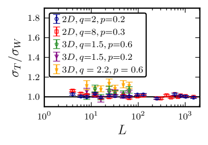
(b)

Figure 1: Monte Carlo estimates of $\mu_{T}/\mu_{W}$ (left) and $\sigma_{T}/\sigma_{W}$ (right) for the off-critical random-cluster model with $d=2,3$, with various cluster fugacities $q$ and bond densities $p$. Error bars corresponding to one standard error are shown.

Analogously, in order to test Conjecture 2.5, Fig. 1(b) plots Monte Carlo estimates of $\sigma_{T}/\sigma_{W}$ for $d=2,3$, with a variety of $q$ values, and off-critical $p$ values, with $\sigma_{W}$ given by (2.17). The agreement is again excellent. The solid black line in Fig. 1(b) again corresponds to the case $q=1$, for which $C(p,q,d)=1$ identically. It is again conceivable, based on Fig. 1(b), that $C(p,q,d)=1$ for all off-critical parameter choices $(p,q,d)$.

3.2 Criticality

In this section, we consider $\mu_{T}$ and $\sigma_{T}$ at criticality when $q\leq q_{\ast}$. We begin by providing numerical evidence in support of Conjecture 2.6. Recall that for $q=1$, we have from (2.16) and (2.17) that $\mu_{T}/\sigma_{T}\sim C\ln(L)$ as $L\to\infty$, with $C>0$. It is therefore natural to ask whether the ratio $\mu_{T}/\sigma_{T}$ continues to behave as a simple function of $\ln(L)$ when $q>1$. We therefore present in Fig. 2 a log-log plot of the ratio $\mu_{T}/\sigma_{T}$ vs $\ln(L)$, for various critical random-cluster model instances in two and three dimensions. Except for $q=q_{\ast}=4$ in two dimensions, we observe that $\mu_{T}/\sigma_{T}$ appears to become asymptotic to a straight line with positive slope, on a log-log scale. It appears that the ratio approaches either a constant or weakly increases with $L$ at $d=2$ and $q=q_{\ast}=4$. Similarly, in three dimensions, we observe that $\mu_{T}/\sigma_{T}$ appears to increase more slowly in $L$ as $q$ approaches $q_{\ast}$. These observations are consistent with the following possible scenario: $\mu_{T}/\sigma_{T}\sim\ln(L)^{w}$ as $L\to\infty$ with an exponent $w$ that equals 1 at $q=1$ and which decreases monotonically with $q$ before finally vanishing at $q=q_{\ast}$. Regardless, we conclude that $\mu_{T}/\sigma_{T}$ diverges with $L$ at criticality when $q<q_{\ast}$, which supports Conjecture 2.6.

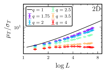
Figure 2: Monte Carlo estimates of $\mu_{T}/\sigma_{T}$ for the critical random-cluster model with $d=2$ (left) and $d=3$ (right), with various cluster fugacities $q\leq q_{\ast}$. Error bars corresponding to one standard error are shown.

We next consider $\sigma_{T}/\sigma_{W}$. Fig. 3 plots $\sigma_{T}/\sigma_{W}$ for $d=2,3$ with various values of $q\leq q_{\ast}$. It is clear that $\sigma_{T}/\sigma_{W}\to\infty$, which strongly suggests that Conjecture 2.5 cannot be extended to $p=p_{\mathrm{c}}$. As we discuss in more detail in Section 3.4, the ratio $\sigma_{T}/\sigma_{W}$ appears to grow at least as fast as $\ln(L)$. Combining this observation, together with (2.16) and (2.17), with the above observation that $\mu_{T}/\sigma_{T}$ diverges, implies that $\mu_{T}/\mu_{W}$ also diverges, which also rules out the possibility that Conjecture 2.4 extends to $p=p_{\mathrm{c}}$. Direct numerical data for the ratio $\mu_{T}/\mu_{W}$ support this conclusion.

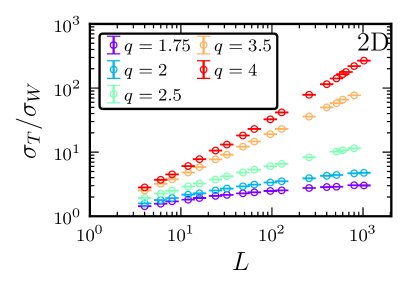
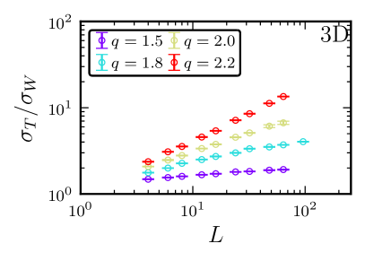
Figure 3: Monte Carlo estimates of $\sigma_{T}/\sigma_{W}$ for the critical random-cluster model with $d=2$ (left) and $d=3$ (right), with various cluster fugacities $q\leq q_{\ast}$. Error bars corresponding to one standard error are shown.

3.3 Variance and relaxation time

We now provide evidence in support of Conjecture 2.8, in both the critical and off-critical cases. Let $(X_{t})_{t\in\mathbb{N}}$ be a stationary FK heat-bath process, and define $(\mathcal{N}_{t})_{t\in\mathbb{N}}$ via $\mathcal{N}_{t}=\mathcal{N}(X_{t})$, where $\mathcal{N}(A)=|A|$ is the number of occupied edges. Since $\mathcal{N}$ is a strictly increasing function, Proposition A.1 in Appendix A implies that

$$\rho_{\mathcal{N}}(t):=\frac{\operatorname{cov}(\mathcal{N}_{0},\mathcal{N}_{t})}{\operatorname{var}(\mathcal{N}_{0})}\sim Ce^{-t/t_{\exp}},\qquad t\to\infty,$$ (3.1)

for some (parameter-dependent) constant $C>0$. Assuming the validity of Conjecture 2.8, it follows from (3.1) that

$$\ln\rho_{\mathcal{N}}(k\,\sigma_{T})\sim-\frac{\pi}{\sqrt{6}}k$$ (3.2)

as $k$ and $L$ tend to infinity.

For a given time lag $t$, we estimated $\rho_{\mathcal{N}}(t)$ by performing around 100 independent simulations, estimating $\rho_{\mathcal{N}}(t)$ from each simulation using the standard time series estimator (see e.g. (Sokal97, , Equation (3.9))), and then calculating the sample mean over independent runs to obtain our final estimate of $\rho_{\mathcal{N}}(t)$. Fig. 4 plots the resulting estimates of $\rho_{\mathcal{N}}(k\,\sigma_{T})$ versus $k$, for a variety of values of $q$, $p$ and $L$. The data collapse evident from the figure clearly supports the expectation (3.2), and therefore provides direct evidence to support Conjecture 2.8.

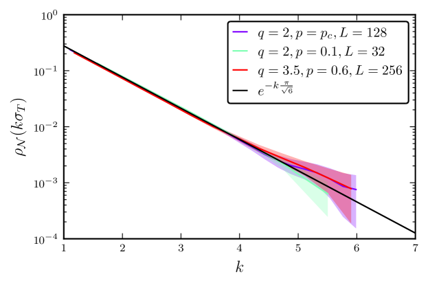
Figure 4: Monte Carlo estimates of $\ln\rho_{\mathcal{N}}(\sigma_{T}\,k)$ for the random-cluster model with $d=2$, and various values of $q<q_{\ast}$, $p$ and $L$. The pairs $(q,p)=(2,0.1)$ and $(q,p)=(3.5,0.6)$ are off-critical. The filled area enclosing the curves correspond to one standard error.

To further test Conjecture 2.8, we used (3.1) to directly estimate $t_{\exp}$, and then compared these estimates with our estimates of $\sigma_{T}$. To estimate $t_{\exp}$ from an estimate of $\rho_{\mathcal{N}}(t)$, we fitted a linear function $a-t/b$ to the data for $(t,\ln\rho_{\mathcal{N}}(t))$, with appropriate cutoffs imposed at both small $t$ (to avoid the pre-asymptotic regime) and large $t$ (to reduce statistical noise). Using these estimates, Fig. 5 shows the $L$ dependence of the ratio $\sigma_{T}/t_{\exp}$ for a variety of critical and off-critical $(p,q)$ pairs, with $q<q_{\ast}$. The solid black line corresponds to the asymptote $\pi/\sqrt{6}$ predicted by Conjecture 2.8. The data collapse is clearly excellent, lending further strong support to the conjecture.

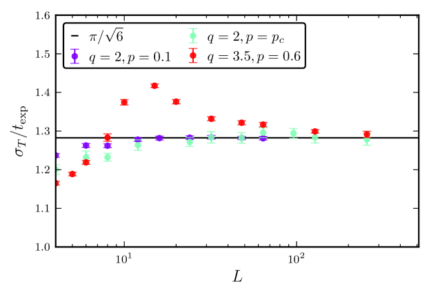
Figure 5: Monte Carlo estimates of $\sigma_{T}/t_{\exp}$ for the random-cluster model with $d=2$, and various values of $q<q_{\ast}$, $p$ and $L$. The pairs $(q,p)=(2,0.1)$ and $(q,p)=(3.5,0.6)$ are off-critical. The solid black line corresponds to the horizontal line $\pi/\sqrt{6}$. Error bars corresponding to one standard error are shown.

3.4 Dynamic critical exponents

We now briefly discuss a practical application of Conjecture 2.8. Assuming the validity of Conjectures 2.5 and 2.8, and combining them with (2.17), confirms the intuition mentioned in Section 2.4 that $t_{\exp}\sim L^{d}$ off criticality. Moreover, a closer inspection of the data in Fig. 3 suggests that, at least for sufficiently large $q<q_{\ast}$, we have $\sigma_{T}/\sigma_{W}\sim L^{z}$ for some exponent $z=z(q,d)>0$. Under the assumption of Conjecture 2.8, this is then equivalent to $t_{\exp}\sim L^{d+z}$. This behaviour, which is precisely the phenomenon of critical slowing-down, is expected on physical grounds Sokal97 to occur generically at $p=p_{\mathrm{c}}$ when $q<q_{\ast}$. The exponent $z$, controlling the divergence of $t_{\exp}/L^{d}$ at continuous phase transitions, is an example of a dynamic critical exponent. It is often denoted $z_{\exp}$ in the literature Sokal97 . While being of considerable physical and practical significance, the precise estimation of $z_{\exp}$, even via simulation, is a highly non-trivial task. However, if Conjecture 2.8 holds, then $z_{\exp}$ for the FK heat-bath process can be estimated efficiently and reliably by considering the more tractable problem of the asymptotics of $\sigma_{T}$. For clarity, we denote the exponent governing the critical asymptotics of $\sigma_{T}/L^{d}$ by $z_{T}$.

So motivated, we considered a number of $d$ and $q<q_{\ast}$ values, and fitted $\sigma_{T}/L^{d}$ to both power-law and logarithmic finite-size scaling ansätze, $aL^{z}+b$ and $a\ln(L)+b$, both with $b$ free and fixed to zero. For a given ansatz, the quality of the fit was studied as we varied the lower cutoff on the $L$ values included in the fits. Table 1 summarises our best estimates for $z_{T}$, chosen to be the estimate resulting from the ansatz that yielded the highest confidence level, and stable estimates with respect to a variation of the lower cutoff. For comparison, we also present corresponding values of $\alpha/\nu$, since a Li-Sokal type bound DengGaroniSokal07_sweeny implies that $z_{\exp}\geq\alpha/\nu$. Here $\alpha$ and $\nu$ are the standard static critical exponents governing the specific heat and correlation length, respectively. For $d=2$, conjectured exact expressions for $\alpha$ and $\nu$ follow from the hyperscaling relation $d\nu=2-\alpha$, the identification of $1/\nu$ with the renormalization group thermal exponent, and (NienhuisJSP84, , Equation (3.37)). For $d=3$, the reported values of $\alpha/\nu$ correspond to the estimates presented in DengGaroniMachtaOssolaPolinSokal07 .

$d$	$q$	$\alpha/\nu$	$z_{T}$
$2$	$1.75$	$-0.1093$	$0(\ln)$
$2$	$2$	$0(\ln)$	$0(\ln)$
$2$	$2.5$	$0.2036$	$0.315(3)$
$2$	$3$	$0.4000$	$0.491(4)$
$2$	$3.5$	$0.6101$	$0.662(2)$
$3$	$1.5$	$-0.32(4)$	$0.090(6)$
$3$	$1.8$	$-0.15(5)$	$0.233(4)$
$3$	$2$	$0.174(1)$	$0.435(9)$
$3$	$2.2$	$0.50(4)$	$0.646(5)$

Table 1: Estimated critical exponent $z_{T}$ for a variety of values of $d$ and $q<q_{\ast}$. If Conjecture 2.8 holds, then $z_{T}=z_{\exp}$.

4 Limiting Distribution

We now turn our attention to the limiting distribution of the coupling time, and provide numerical evidence in support of Conjecture 2.7. To ease notation, in this section we introduce the standardized variable

$$S:=(T-\mu_{T})/\sigma_{T}.$$ (4.1)

4.1 Off criticality

In this section we present evidence supporting Conjecture 2.7 in the off-critical case. We defer discussion of the critical case until Section 4.2.

Fig. 6 compares histograms of $S$ with the probability density function corresponding to (2.19). The left panel corresponds to $d=2$ and $q=8$ at $p=0.3<p_{\mathrm{c}}(8,2)$. The right panel corresponds to $d=3$ and $q=1.5$ at $p=0.2$; for reference, it is estimated DengGaroniSokalZhou that $p_{\mathrm{c}}(1.5,3)=0.31157497(59)$. The agreement is clearly excellent, providing strong support for Conjecture 2.7.

Figure 6: Histograms of off-critical $S$, with parameters as specified in the figure. The histograms are based on $19,000$ independent samples for $d=2$ and $11,000$ for $d=3$. Here $p(s)$ denotes the probability density function of $S$. For comparison, the solid green line shows the probability density function corresponding to (2.19).

We emphasize that the theoretical curve shown in Fig. 6 does not correspond to a fit to the data; the distribution $G(x)$ does not possess any free parameters. In order to obtain a quantitative measure of how well the limiting distribution of $S$ is described by $G(x)$, we therefore considered the three-parameter family of distributions known as the Generalized Extreme Value distribution (GEV), defined by the distribution function

$$F_{\rm GEV}\big{(}x;\xi,\eta,\theta\big{)}:=\begin{cases}e^{-e^{-(x-\eta)/\theta}}&\xi=0,\\ e^{-\big{(}1+\xi(x-\eta)/\theta\big{)}^{-1/\xi}}&\xi\neq 0,\end{cases}$$ (4.2)

where $\xi,\eta\in\mathbb{R}$ and $\theta>0$. The support of $F_{\mathrm{GEV}}$ is $\mathbb{R}$ for $\xi=0$, $[\eta-\theta/\xi,\infty)$ for $\xi>0$, and $(-\infty,\eta-\theta/\xi]$ for $\xi<0$. The case $\xi=0$ corresponds to the Gumbel family of distributions, and the specific values

$$\xi=0,\quad\eta=-\frac{\gamma\sqrt{6}}{\pi}=-0.45005320754\ldots,\quad\theta=\frac{\sqrt{6}}{\pi}=0.77969780123\ldots$$ (4.3)

correspond to $G(x)$ as given in (2.19).

Our consideration of $F_{\mathrm{GEV}}$ can be motivated as follows. Consider an iid sequence of random variables $X_{1},X_{2},\ldots$ and let $M_{n}:=\max\{X_{1},\ldots,X_{n}\}$. The extremal types theorem (see e.g. (LeadbetterLindgrenRootzen83, , Theorem 1.4.2)) states that if the sequence $M_{n}$, appropriately standardized, has a non-degenerate limit, then the limit must be a GEV distribution. To relate this observation to the coupling time, we can envision coarse-graining the lattice into regions of size much larger than the spatial correlation length, which is finite off criticality. To each such region we can assign a local coupling time, defined to be the last time before $T$ that the state (occupied or unoccupied) of each edge in that region is the same in the top and bottom chains. Since the correlations between regions are weak, as a first approximation one can envision the local coupling times as independent. Moreover, the coupling time of the system, $T$, is the maximum of these local coupling times. It is therefore natural to expect that if an appropriate standardization of $T$ converges to a non-degenerate limit as $L\to\infty$, then the limit should be of the form (4.2).

We therefore fitted the ansatz (4.2) to our data for $S$, and computed maximum likelihood-estimates of the parameters $\xi,\eta,\theta$. For $d=2$, $q=8$, $p=0.3$ and $L=128$, (left panel of Fig. 6) we obtain

$$\xi=0.01(1)\quad\eta=-0.45(1)\quad\theta=0.77(1),$$ (4.4)

based on $19000$ independent samples, and with error bars are computed via bootstrap re-sampling Young15 . These estimates are in perfect agreement with the parameter values corresponding to $G(x)$. Similarly, for $d=3$, $q=1.5$, $p=0.2$ and $L=64$ (right panel in Fig. 6), we obtain

$$\xi=0.01(1)\quad\eta=-0.45(2)\quad\theta=0.78(1)$$ (4.5)

based on $11000$ samples. Finally, we also considered $d=3$, $q=2.2$ and $p=0.6$, which is expected to be in the supercritical regime DengGaroniSokalZhou , and obtained

$$\xi=0.00(1)\quad\eta=-0.45(2)\quad\theta=0.79(1),$$ (4.6)

based on $11000$ samples. In each case, the estimates of the GEV parameters are entirely consistent with the parameter values in (4.3) corresponding to $G(x)$, as predicted in Conjecture 2.7.

4.2 Criticality

Although we have observed that $\mu_{T}$ and $\sigma_{T}$ display non-trivial $L$ dependencies when $p=p_{\mathrm{c}}$, we now present evidence that Conjecture 2.7 is valid at $p=p_{\mathrm{c}}$ when $q<q_{\ast}$.

Fig. 7 compares histograms of $S$ with the probability density function corresponding to (2.19). The left panel corresponds to $d=2$ and $q=3.5$, while the right panel corresponds to $d=3$ and $q=1.5$. The agreement is clearly excellent, providing strong support for Conjecture 2.7.

Figure 7: Histograms of $S$ at criticality, with parameters as specified in the figure. The histograms are based on $15,000$ independent samples for $d=2$ and $10,000$ for $d=3$. Here $p(s)$ denotes the probability density function of $S$. For comparison, the solid green line shows the probability density function corresponding to (2.19).

Analogous to our discussion of the off-critical case in Section 4.1, we can obtain a more quantitative test of the agreement between the limiting distribution of $S$ and (2.19) by fitting the GEV distribution, (4.2). We considered a number of values of $q<q_{\ast}$ with $d=2,3$, and our results are summarized in Table 2. The estimates of the GEV parameters $\eta,\theta,\xi$ are in good agreement with the parameter values (4.3) corresponding to $G(x)$. The combination of these numerical results strongly support the validity of Conjecture 2.7.

$d$	$q$	$L$	$\eta$	$\theta$	$\xi$	$N_{\mathrm{s}}$
2	$1.75$	$1024$	$-0.45(3)$	$0.80(2)$	$-0.02(2)$	$3360$
2	$1.75$	$512$	$-0.45(2)$	$0.79(1)$	$-0.01(2)$	$9800$
2	$2.00$	$512$	$-0.45(2)$	$0.78(1)$	$0.00(1)$	$9000$
2	$2.00$	$800$	$-0.45(2)$	$0.80(1)$	$-0.02(1)$	$9000$
2	$2.50$	$512$	$-0.45(2)$	$0.79(2)$	$-0.01(1)$	$9000$
2	$3.00$	$512$	$-0.45(2)$	$0.78(1)$	$0.01(1)$	$9000$
2	$3.50$	$512$	$-0.46(2)$	$0.77(1)$	$0.02(2)$	$8990$
2	$3.50$	$800$	$-0.46(1)$	$0.77(1)$	$0.01(1)$	$15730$
3	$1.5$	$64$	$-0.45(1)$	$0.78(1)$	$0.01(2)$	$10000$
3	$1.8$	$64$	$-0.44(1)$	$0.81(1)$	$0.03(1)$	$10000$
3	$2.0$	$64$	$-0.45(2)$	$0.80(3)$	$0.03(3)$	$700$
3	$2.2$	$64$	$-0.44(1)$	$0.80(1)$	$0.03(1)$	$10000$

Table 2: Parameter estimates obtained by fitting the GEV distribution (4.2) to the empirical distribution for $S$ at $p=p_{\mathrm{c}}$, for various choices of $q<q_{\ast}$. Here $N_{\mathrm{s}}$ denotes the number of samples. Error bars correspond to one standard error.

We conclude this section with some comments on the case of $p=p_{\mathrm{c}}$ and $q\geq q_{\ast}$, which is excluded from our statement of Conjecture 2.7. Because of the slow mixing inherent at discontinuous phase transitions, it is much more difficult to obtain accurate simulation results at $p=p_{\mathrm{c}}$ when $q>q_{\ast}$. We did however perform a simulation study for $d=2$ at $p_{\mathrm{c}}$ for $q=5>q_{\ast}$. While it does appear that the standardized variable $S$ again converges to a non-degenerate limit, it appears that this limit is not $G(x)$. To illustrate this, we generated 10,000 samples of $T$ with $L=256$, and obtained the following GEV parameter estimates: $\xi=0.19(2)$, $\eta=-0.49(2)$, $\theta=0.62(1)$. The deviation of $\xi$ away from the Gumbel value $\xi=0$ seems to provide strong evidence that Conjecture 2.7 cannot be extended to the case of $p=p_{\mathrm{c}}$ when $q>q_{\ast}$.

The case $q=q_{\ast}$ is more subtle. In this case, it is not slow mixing that constitutes an impediment, but rather the notorious issue of multiplicative logarithms arising in finite-size scaling ansätze. We simulated the case $d=2$ and $q=q_{\ast}=4$ at $p=p_{\mathrm{c}}$, at a variety of different $L$ values. We again observe that the distribution of $S$ appears to converge to a non-degenerate limit. The GEV distribution was fitted to the data for $S$, and the corresponding estimates for $\eta,\theta,\xi$ are reported in Table 3. The resulting estimates of $\theta$ and $\xi$ are not consistent with the values corresponding to $G(x)$. In particular, the estimates suggest $\xi$ is strictly positive, which would rule out a Gumbel limit law. Therefore, based on these estimates, there does not appear to be any evidence suggesting Conjecture 2.7 can be extended to the case of $(p,q)=(p_{\mathrm{c}},q_{\ast})$. However, the discrepancies of these parameter estimates with the values corresponding to $G(x)$ are relatively small. Therefore, we also believe that there is insufficient evidence to conclude that the distribution of $S$ at $(p,q)=(p_{\mathrm{c}},q_{\ast})$ is actually different to $G(x)$. Determining the limiting distribution of $S$ at $(p,q)=(p_{\mathrm{c}},q_{\ast})$ therefore remains an open problem.

$L$	$\eta$	$\theta$	$\xi$	$N_{\mathrm{s}}$
$128$	$-0.46(2)$	$0.73(1)$	$0.05(2)$	$8990$
$256$	$-0.47(2)$	$0.71(1)$	$0.08(2)$	$9000$
$512$	$-0.47(1)$	$0.73(1)$	$0.06(1)$	$18940$
$800$	$-0.47(1)$	$0.72(1)$	$0.07(1)$	$20000$
$1024$	$-0.47(2)$	$0.72(1)$	$0.07(1)$	$9850$

Table 3: Parameter estimates obtained by fitting the GEV distribution (4.2) to the empirical distribution for $S$ at $(p,q)=(p_{\mathrm{c}},q_{\ast})$ and $d=2$, for various choices of $L$. Here $N_{\mathrm{s}}$ denotes the number of samples. Error bars correspond to one standard error.

5 Arbitrary graphs

In this section, we consider the FK heat-bath process on arbitrary graphs, and prove Theorem 2.1.

Proof of Theorem 2.1.

Consider the FK heat-bath coupling on a finite connected graph $G=(V,E)$ with $|E|=m\geq 1$, and let

$$d(t):=\max_{A\subseteq E}\|P^{t}(A,\cdot)-\phi\|_{\mathrm{TV}}.$$ (5.1)

It follows from (ProppWilson96, , Theorem 5) and (LevinPeresWilmer09, , Equation (4.24)) that

$$d(t)\leq\mathbb{P}(T>t)\leq 2\,(m+1)\,d(t),$$ (5.2)

for any $t\in\mathbb{N}$. Combining the lower bound in (5.2) with (LevinPeresWilmer09, , Equation (12.13)) yields the stated lower bound for the tail distribution:

$$\mathbb{P}(T>t)\geq d(t)\geq\frac{e^{-t/t_{\exp}}}{2}.$$

Similarly, combining (5.2) with Markov’s inequality implies

$$\mathbb{E}(T)\geq(t_{\mathrm{mix}}-1)\,\mathbb{P}(T>t_{\mathrm{mix}}-1)\geq(t_{\mathrm{mix}}-1)d(t_{\mathrm{mix}}-1)\geq\frac{(t_{\mathrm{mix}}-1)}{4}.$$

This establishes the stated lower bounds.

We now consider the upper bounds. Let $M\in(1,\infty)$ be such that

$$\mathbb{P}(T>l\,M)\leq 2^{-l},\qquad\text{for all }l\in\mathbb{N}.$$ (5.3)

Then for $k\in\{0,1\}$ we have

$$\sum_{t=0}^{\infty}t^{k}\,\mathbb{P}(T>t) \leq\sum_{l=0}^{\infty}\sum_{t=l\lceil M\rceil}^{(l+1)\lceil M\rceil-1}t^{k}\,\mathbb{P}(T>l\,M)$$

$$\leq\sum_{l=0}^{\infty}\sum_{t=l\lceil M\rceil}^{(l+1)\lceil M\rceil-1}t^{k}\,2^{-l}$$

$$=(k+2)\lceil M\rceil^{k+1}-k\,\lceil M\rceil.$$

The $k=0$ case then immediately yields an upper bound for $\mathbb{E}(T)$, via

$$\mathbb{E}(T)=\sum_{t=0}^{\infty}\mathbb{P}(T>t)\leq 2\,\lceil M\rceil\leq 4\,M.$$ (5.4)

Similarly, standard manipulations of probability generating functions (see e.g. (Feller68, , Chapter XI)) show that

$$\mathbb{E}\,[T(T-1)]=2\sum_{t=0}^{\infty}t\,\mathbb{P}(T>t),$$ (5.5)

and so the $k=1$ case yields

$$\operatorname{var}(T)\leq\mathbb{E}[T(T-1)]+\mathbb{E}(T)\leq 6\lceil M\rceil^{2},$$ (5.6)

which implies

$$\sqrt{\operatorname{var}(T)}\leq\sqrt{6}(M+1)\leq 2\sqrt{6}\,M\leq 5\,M.$$ (5.7)

We now determine suitable choices of $M$ for which (5.3) holds. Since the bound is trivial for $l=0$, we assume $l\geq 1$. We begin by considering bounds in terms of $t_{\exp}$. Letting $\phi_{\min}:=\min\{\phi(A):A\subseteq E\}$, and combining (LevinPeresWilmer09, , Lemma 6.13) and (LevinPeresWilmer09, , Equation (12.11)) with (5.2) yields

$$\mathbb{P}(T>t)\leq 2(m+1)\,d(t)\leq\frac{2(m+1)}{\phi_{\min}}e^{-t/t_{\exp}}\leq 2\,(m+1)\,\psi^{m}\,e^{-t/t_{\exp}},$$ (5.8)

where in the last step we applied Lemma 5.1. Since $\ln[2(m+1)]\leq 2m$, this immediately yields the stated upper bound for $\mathbb{P}(T>t)$. Likewise, since ${\log_{2}[2(m+1)])\leq 2m}$, if we set $M=[\log_{2}(\psi)+3]m\,t_{\exp}$ then it follows from (5.8) that

$$\log_{2}\mathbb{P}(T>l\,M) \leq[\log_{2}(\psi)+2]m-l[\log_{2}(\psi)+3]m$$

$$=-(l-1)[2+\log_{2}(\psi)]m-m\,l$$

$$\leq-m\,l$$

$$\leq-l,$$

and so (5.3) holds. Inserting this choice of $M$ into (5.5) and (5.7) then yields the stated upper bounds for $\mathbb{E}(T)$ and $\sqrt{\operatorname{var}(T)}$ in terms of $t_{\exp}$.

Finally, we consider bounds in terms of $t_{\mathrm{mix}}$. Combining (5.2) with (LevinPeresWilmer09, , Equation (4.35)) we obtain

$$\mathbb{P}(T>t)\leq 2(m+1)\,d(t)\leq 4\,m\,d(t)\leq 2^{\log_{2}(4m)-\lfloor t/t_{\mathrm{mix}}\rfloor}$$

Setting $M=3\log_{2}(4m)\,t_{\mathrm{mix}}$, it follows that

$$\log_{2}\mathbb{P}(T>l\,M) \leq\log_{2}(4m)-3\log_{2}(4m)l+1$$

$$=[1-(2l-1)\log_{2}(4m)]-\log_{2}(4m)\,l$$

$$\leq-\log_{2}(4m)\,l$$

$$\leq-l,$$

which implies that (5.3) holds. Inserting this choice of $M$ into (5.5) and (5.7) then yields the stated upper bounds for $\mathbb{E}(T)$ and $\sqrt{\operatorname{var}(T)}$ in terms of $t_{\mathrm{mix}}$.

∎

Lemma 5.1.

Consider the FK model with $q\geq 1$ and $p\in(0,1)$, on a finite connected graph $G=(V,E)$ with $m$ edges, and let $\phi_{\min}:=\min\{\phi(A):A\subseteq E\}$. Then

$$\phi_{\min}\geq\left(\frac{p(1-p)}{q^{2}}\right)^{m}.$$

Proof.

Since

$$\sum_{A\subseteq E}p^{|A|}(1-p)^{m-|A|}q^{k(A)}\leq q^{n}\sum_{A\subseteq E}p^{|A|}(1-p)^{m-|A|}=q^{n},$$

for any $A\subseteq E$ we have

$$\phi(A)\geq p^{|A|}(1-p)^{m-|A|}q^{k(A)-n}\geq p^{m}(1-p)^{m}q^{-n}.$$

The stated result then follows since $G$ being connected implies $n\leq m+1\leq 2m$. ∎

6 The cycle

In this section, we consider the FK heat-bath coupling, with parameters $p\in(0,1)$ and $q\geq 1$, on the graph $\mathbb{Z}_{L}$, and prove Theorem 2.3. We begin, in Section 6.1, by showing that $T$ equals $W$ with high probability, as $L\to\infty$. This observation is then used in Section 6.2 to prove Parts (i) and (ii), of Theorem 2.3, and again in Section 6.3 to prove Part (iii). Finally, in Section 6.4, we prove Part (iv).

6.1 Asymptotic Coupon Collector Behaviour

For each $e\in E$, define

$$H(e)=\sup\{t\leq W:\mathcal{E}_{t}=e\}.$$

We refer to the time $H(e)$ as the last visit to $e$. Let $(H_{i})_{i=1}^{m}$ denote the sequence of the $H(e)$, arranged in increasing order. In particular, $H_{1}$ is the first time that a last visit occurs. And likewise, $H_{i}$ is the time that the $i$th last visit occurs.

Proposition 6.1.

Consider the FK heat-bath coupling on $\mathbb{Z}_{L}$ with $p\in(0,1)$ and $q\geq 1$. There exists $\epsilon>0$ such that $\mathbb{P}(T=W)=1-O(L^{-\epsilon})$.

Proof.

Fix $p\in(0,1)$ and $q\geq 1$, and let $a_{L}:=\left\lfloor\ln L\right\rfloor$. Let $\mathcal{P}_{j}$ be the event that the edge $\mathcal{E}_{H_{j}}$ is pivotal in the top process at time $H_{j}-1$. By monotonicity, whenever an edge is pivotal to the top chain, it is also pivotal to the bottom chain. Lemma 6.2 implies that there exists $\omega>0$ such that

$$\mathbb{P}(T>W)=\mathbb{P}\left(T>W\bigg{|}\bigcap_{j=1}^{a_{L}}\mathcal{P}_{j}\right)+O(L^{-\omega}).$$ (6.1)

Now suppose $\cap_{j=1}^{a_{L}}\mathcal{P}_{j}$ occurs, and let $1\leq i\leq a_{L}$. If $U_{H_{i}}\leq\tilde{p}$, then $\mathcal{E}_{H_{i}}\in\mathcal{B}_{t}$ and $\mathcal{E}_{H_{i}}\in\mathcal{T}_{t}$ for all $t\in[H_{i},W]$, while if $U_{H_{i}}>\tilde{p}$ then $\mathcal{E}_{H_{i}}\not\in\mathcal{B}_{t}$ and $\mathcal{E}_{H_{i}}\not\in\mathcal{T}_{t}$ for all $t\in[H_{i},W]$. Consequently, on $\mathbb{Z}_{L}$, if $U_{H_{i}}>\tilde{p}$, then every edge $e\neq\mathcal{E}_{H_{i}}$ is pivotal to $\mathcal{T}_{t}$ and $\mathcal{B}_{t}$, for all $t\in(H_{i},W]$, so that after any update of such an edge in this time window, its state (occupied or unoccupied) in the top and bottom chain will agree. Since each $e\in E\setminus\{\mathcal{E}_{H_{1}},\ldots,\mathcal{E}_{H_{i}}\}$ must be updated in $(H_{i},W]$, this implies that the top and bottom chains agree at time $W$, and so $T\leq W$. It follows that $T>W$ can occur only if $U_{H_{i}}\leq\tilde{p}$ for each $1\leq i\leq a_{L}$, and so

$$\mathbb{P}\left(T>W\bigg{|}\bigcap_{j=1}^{a_{L}}\mathcal{P}_{j}\right)\leq\tilde{p}^{a_{L}}\leq\frac{L^{\ln\tilde{p}}}{\tilde{p}}.$$ (6.2)

Since $p\in(0,1)$, we have $\tilde{p}\in(0,1)$, and so $\ln(\tilde{p})<0$. Choosing $\epsilon=\min\{\omega,-\ln\tilde{p}\}$, and combining (6.1) and (6.2), we therefore obtain

$$\mathbb{P}(T>W)=O(L^{-\epsilon}).$$

Combining this observation with (2.20) yields the stated result. ∎

Lemma 6.2.

Consider the top process on $\mathbb{Z}_{L}$, with fixed $p\in(0,1)$ and $q\geq 1$. Let $\mathcal{P}_{j}$ be the event that the edge $\mathcal{E}_{H_{j}}$ is pivotal at time $H_{j}-1$, and let $a_{L}=\left\lfloor\ln L\right\rfloor$. Then there exists $\omega>0$ such that

$$\mathbb{P}\left(\bigcup_{j=1}^{a_{L}}\mathcal{P}_{j}^{c}\right)=O(L^{-\omega}),\qquad L\to\infty.$$

Proof.

Let $R_{t}:=\{e\in E:\mathcal{E}_{s}=e\textrm{ for some }s\leq t\}$, the set of distinct edges visited up to time $t$. Let $\mathcal{D}=\{|R_{H_{1}}|>a_{L}\}$ be the event that more than $a_{L}$ distinct edges have been visited by time $H_{1}$. If $\mathcal{D}$ holds, then it also holds that more than $a_{L}$ distinct edges have been visited by time $H_{j}$, for any $j\geq 1$. Fix $1\leq j\leq L$ and $p,\xi\in(0,1)$, and define $\mathcal{A}_{j}$ to be the event that at least $\xi(1-p)a_{L}$ edges are unoccupied at time $H_{j}-1$. For any choice of $\xi,p\in(0,1)$, we have $\xi(1-p)a_{L}\geq 2$ for all sufficiently large $L$; let $L$ be so chosen in what follows. Then, if $\mathcal{A}_{j}$ occurs, there are at least 2 unoccupied edges at time $H_{j}-1$, which in turn means that all edges are pivotal at time $H_{j}-1$. Therefore, $\mathcal{A}_{j}\subseteq\mathcal{P}_{j}$.

Let $\mathcal{W}$ denote the set of the first $a_{L}$ distinct edges visited by $(\mathcal{E}_{t})_{t\in\mathbb{N}^{+}}$. On $\mathcal{D}$, the edges in $\mathcal{W}$ are all visited prior to $H_{j}$. Denote the times of last visit to the edges in $\mathcal{W}$, prior to $H_{j}$, by $M_{1}<M_{2}<\ldots<M_{a_{L}}$, and let $1\leq i\leq a_{L}$. Since $p\geq\tilde{p}$, if $U_{M_{i}}>p$, then regardless of the structure of $\mathcal{T}_{M_{i}-1}$, we have $\mathcal{E}_{M_{i}}\not\in\mathcal{T}_{M_{i}}$. It follows that if $X_{i}=\mathbf{1}(U_{M_{i}}>p)$, then $\mathbb{P}(\mathcal{E}_{M_{i}}\not\in\mathcal{T}_{M_{i}})\geq\mathbb{P}(X_{i}=1)=(1-p)$. Therefore, Chernoff’s bound (MitzenmacherUpfal05, , Equation (4.5)) implies

$$\mathbb{P}\left(\mathcal{P}_{j}^{c}|\mathcal{D}\right)\leq\mathbb{P}\left(\mathcal{A}_{j}^{c}|\mathcal{D}\right)\leq\mathbb{P}\left(\sum_{i=1}^{a_{L}}X_{i}<\xi(1-p)a_{L}\right)\leq e^{-\gamma a_{L}}$$

with $\gamma=(1-\xi)^{2}(1-p)/2>0$.

Combining this with the union bound gives

$$\mathbb{P}\left(\bigcup_{j=1}^{a_{L}}\mathcal{P}_{j}^{c}\bigg{|}\mathcal{D}\right) \leq\sum_{j=1}^{a_{L}}\mathbb{P}(\mathcal{P}_{j}^{c}|\mathcal{D})$$

$$\leq a_{L}e^{-\gamma a_{L}}$$

$$\leq e^{\gamma}\,\ln(L)\,L^{-\gamma}.$$

It follows that for any $0<\delta<\gamma$ we have

$$\mathbb{P}\left(\bigcup_{j=1}^{a_{L}}\mathcal{P}_{j}^{c}\bigg{|}\mathcal{D}\right)=O(L^{-\delta}).$$

Finally, Lemma B.1 in Appendix B implies that there exists $\varphi>0$ such that

$$\mathbb{P}(\mathcal{D}^{c})=O(L^{-\varphi}).$$

Choosing $\omega=\min\{\delta,\varphi\}$ then implies

$$\mathbb{P}\left(\bigcup_{j=1}^{a_{L}}\mathcal{P}_{j}^{c}\right)=O(L^{-\omega}).$$

Since $\omega>0$, the stated result follows. ∎

6.2 Mean and Variance

Define the sequence of random times $W_{j}$ such that $W_{0}=0$ and for $j\in\mathbb{N}^{+}$

$$W_{j}:=\min\{t>W_{j-1}\,:\,\{\mathcal{E}_{W_{j-1}+1},\ldots,\mathcal{E}_{t}\}=E\}.$$

We define new processes $(\tilde{\mathcal{T}}_{t})_{t\in\mathbb{N}}$ and $(\tilde{\mathcal{B}}_{t})_{t\in\mathbb{N}}$ as follows, which proceed analogously to the top and bottom chains, except that they are restarted at times $W_{j}<T$. More precisely, let $\tilde{\mathcal{T}}_{0}=E$, and for $t\in\mathbb{N}$ set

$$\tilde{\mathcal{T}}_{t+1}=\begin{cases}f(E,\mathcal{E}_{t+1},U_{t+1}),&t=W_{j}\text{ and }T>W_{j},\\ f(\tilde{\mathcal{T}}_{t},\mathcal{E}_{t+1},U_{t+1}),&\text{otherwise.}\end{cases}$$ (6.3)

Similarly, $\tilde{\mathcal{B}}_{0}=\emptyset$, and for $t\in\mathbb{N}$ we set

$$\tilde{\mathcal{B}}_{t+1}=\begin{cases}f(\emptyset,\mathcal{E}_{t+1},U_{t+1}),&t=W_{j}\text{ and }T>W_{j},\\ f(\tilde{\mathcal{B}}_{t},\mathcal{E}_{t+1},U_{t+1}),&\text{otherwise.}\end{cases}$$ (6.4)

By monotonicity, it is clear that for all $t\in\mathbb{N}$ we have

$$\tilde{\mathcal{B}}_{t}\leq\mathcal{B}_{t}\leq\mathcal{T}_{t}\leq\tilde{\mathcal{T}}_{t}.$$ (6.5)

We can now consider the coupling time corresponding to $\tilde{\mathcal{T}}_{t}$ and $\tilde{\mathcal{B}}_{t}$,

$$\tilde{T}:=\min\{t\in\mathbb{N}\,:\,\tilde{\mathcal{T}}_{t}=\tilde{\mathcal{B}}_{t}\}.$$ (6.6)

It follows from (6.5) that $T\leq\tilde{T}$. Combining this with (2.20) implies

$$W\leq T\leq\tilde{T}.$$ (6.7)

Proof of Theorem 2.3, Parts (i) and (ii).

Combining (6.7) and Lemma 6.3 immediately yields $\mathbb{E}(T)\sim\mathbb{E}(W)$, which establishes Part (i).

To establish Part (ii) we note that (6.7) implies

$$\mathbb{E}(W^{2})-(\mathbb{E}\tilde{T})^{2}\leq\operatorname{var}(T)\leq\mathbb{E}(\tilde{T}^{2})-(\mathbb{E}W)^{2},$$

and rearranging, we obtain

$$1-\frac{(\mathbb{E}W)^{2}}{\operatorname{var}(W)}\,\left[\left(\frac{\mathbb{E}\tilde{T}}{\mathbb{E}W}\right)^{2}-1\right]\leq\frac{\operatorname{var}(T)}{\operatorname{var}(W)}\leq\frac{\operatorname{var}(\tilde{T})}{\operatorname{var}(W)}+\frac{(\mathbb{E}W)^{2}}{\operatorname{var}(W)}\,\left[\left(\frac{\mathbb{E}\tilde{T}}{\mathbb{E}W}\right)^{2}-1\right].$$ (6.8)

Lemma 6.3 implies

$$\left[\left(\frac{\mathbb{E}\tilde{T}}{\mathbb{E}W}\right)^{2}-1\right]=O(L^{-\epsilon}),$$ (6.9)

while (2.16) and (2.17) imply

$$\frac{(\mathbb{E}W)^{2}}{\operatorname{var}(W)}=O(\ln^{2}(L)),$$ (6.10)

and so (6.8) yields

$$1\leq\liminf_{L\to\infty}\frac{\operatorname{var}(T)}{\operatorname{var}(W)}\leq\limsup_{L\to\infty}\frac{\operatorname{var}(T)}{\operatorname{var}(W)}\leq\limsup_{L\to\infty}\frac{\operatorname{var}(\tilde{T})}{\operatorname{var}(W)}.$$

Combining this with Part (ii) of Lemma 6.3 then implies that $\operatorname{var}(T)\sim\operatorname{var}(W)$. ∎

Lemma 6.3.

Let $\tilde{T}$ be as defined in (6.6). Then:

1. $\mathbb{E}(\tilde{T})=\mathbb{E}(W)[1+O(L^{-\epsilon})]$.

2. $\limsup_{L\to\infty}\operatorname{var}(\tilde{T})/\operatorname{var}(W)\leq 1$.

Proof.

By construction of the processes $\tilde{\mathcal{B}}_{t}$ and $\tilde{\mathcal{T}}_{t}$, we have $\tilde{T}\in\{W_{1},W_{2},W_{3},\ldots\}$. Defining the random index $J$ via

$$J:=\inf\{j\in\mathbb{N}:\tilde{\mathcal{B}}_{W_{j}}=\tilde{\mathcal{T}}_{W_{j}}\},$$

we therefore have $\tilde{T}=W_{J}$. It follows that

$$\tilde{T}=\sum_{j=1}^{J}Y_{j},$$

where $Y_{j}:=(W_{j}-W_{j-1})$ form an iid sequence of copies of $W_{1}=W$. Moreover, $J$ is geometrically distributed, with success probability $\mathbb{P}(T=W)$. From Proposition 6.1 we therefore obtain

$$\begin{split}\mathbb{E}(J)&=1+O(L^{-\epsilon}),\\ \operatorname{var}(J)&=O(L^{-\epsilon}).\end{split}$$ (6.11)

Let $\mathcal{F}_{t}:=\sigma(\mathcal{E}_{1},U_{1},\ldots,\mathcal{E}_{t},U_{t})$ denote the natural filtration of the auxiliary noise. For each $j\in\mathbb{N}^{+}$, the time $W_{j}$ is a stopping time with respect to $\mathcal{F}_{t}$, and we can define the $\sigma$-algebra $\mathcal{G}_{j}:=\mathcal{F}_{W_{j}}$. Since $W_{j-1}<W_{j}$, the sequence $(\mathcal{G}_{j})_{j\in\mathbb{N}^{+}}$ is a filtration, and moreover, $(Y_{j})_{j\in\mathbb{N}^{+}}$ is adapted to it. It is easily verified that $\sigma(Y_{j})$ and $\mathcal{G}_{j-1}$ are independent, for each $j\in\mathbb{N}^{+}$. Furthermore, $J$ is a stopping time with respect to $(\mathcal{G}_{j})_{j\in\mathbb{N}^{+}}$. It therefore follows from Wald’s first equation (ChowTeicher78, , Theorem 5.3.1) that

$$\mathbb{E}(\tilde{T})=\mathbb{E}(J)\,\mathbb{E}(W).$$ (6.12)

Combining (6.11) with (6.12) yields statement (i).

We now turn to statement (ii). Consider the random variable $\tilde{T}-\mathbb{E}(W)\,J$. We clearly have

$$\tilde{T}-\mathbb{E}(W)\,J=\sum_{j=1}^{J}[Y_{j}-\mathbb{E}(W)],$$

and it follows from (6.12) that $\tilde{T}-\mathbb{E}(W)\,J$ has mean zero. Wald’s second equation (ChowTeicher78, , Theorem 5.3.3) therefore yields

$$\mathbb{E}[(\tilde{T}-\mathbb{E}(W)\,J)^{2}]=\mathbb{E}(J)\,\operatorname{var}(Y_{1}-\mathbb{E}(W))=\mathbb{E}(J)\,\operatorname{var}(W).$$ (6.13)

We can upper-bound $\operatorname{var}(\tilde{T})$ using (6.13) as follows. Fix a parameter $a>1$. Jensen’s inequality implies that for any $b,c\in\mathbb{R}$ we have

$$(b+c)^{2}=\left(\frac{1}{a}ba+\frac{a-1}{a}\frac{ca}{(a-1)}\right)^{2}\leq b^{2}a+c^{2}\frac{a}{(a-1)}.$$ (6.14)

From (6.12) and (6.14) it follows that, for any $a>1$,

$$\begin{split}\operatorname{var}(\tilde{T})&=\mathbb{E}\left(\Big{[}\tilde{T}-\mathbb{E}(W)\mathbb{E}(J)\Big{]}^{2}\right)\\ &=\mathbb{E}\left(\left[(\tilde{T}-\mathbb{E}(W)\,J)+\mathbb{E}(W)(J-\mathbb{E}(J))\right]^{2}\right)\\ &\leq a\,\mathbb{E}\left[\left(\tilde{T}-\mathbb{E}(W)\,J\right)^{2}\right]+\frac{a}{(a-1)}(\mathbb{E}W)^{2}\operatorname{var}(J)\\ &=a\,\mathbb{E}(J)\,\operatorname{var}(W)+\frac{a}{a-1}\,(\mathbb{E}W)^{2}\operatorname{var}(J),\end{split}$$ (6.15)

where the last step follows from (6.13). From (6.10) and (6.11) we therefore obtain that, for any $a>1$,

$$\frac{\operatorname{var}(\tilde{T})}{\operatorname{var}(W)}\leq a\,[1+O(L^{-\epsilon})]+\frac{a}{1-a}\frac{(\mathbb{E}W)^{2}}{\operatorname{var}(W)}O(L^{-\epsilon})\leq a+o(1),$$

and we conclude that

$$\limsup_{L\to\infty}\frac{\operatorname{var}(\tilde{T})}{\operatorname{var}(W)}\leq a.$$ (6.16)

Finally, since (6.16) holds for all $a>1$, we in fact have

$$\limsup_{L\to\infty}\frac{\operatorname{var}(\tilde{T})}{\operatorname{var}(W)}\leq 1,$$

as claimed. ∎

6.3 Distribution

By combining Proposition 6.1 with Parts (i) and (ii) of Theorem 2.3, we can now prove Part (iii).

Proof of Theorem 2.3, Part (iii).

Fix $q\geq 1$ and $p\in(0,1)$, and let $\mathbb{P}_{L}$ denote the corresponding measure for the FK heat-bath coupling on $\mathbb{Z}_{L}$, with analogous notation for expectation and variance. Define the sequences $g_{L}:=\mathbb{E}_{L}(T)$, $\gamma_{L}:=\mathbb{E}_{L}(W)$, $h_{L}:=\sqrt{\operatorname{var}_{L}(T)}$ and $\eta_{L}:=\sqrt{\operatorname{var}_{L}(W)}$. Proposition 6.1 implies that for any fixed $x\in\mathbb{R}$, we have

$$\begin{split}\mathbb{P}_{L}[T\leq g_{L}+x\,h_{L}]&=\mathbb{P}_{L}[W\leq g_{L}+x\,h_{L}|T=W]+O(L^{-\epsilon})\\ &=\mathbb{P}_{L}[W\leq g_{L}+x\,h_{L}]+O(L^{-\epsilon}).\end{split}$$ (6.17)

Since Parts (i) and (ii) of Theorem 2.3 imply, respectively, that $\gamma_{L}\sim g_{L}$ and $\eta_{L}\sim h_{L}$, the stated result follows from (6.17) via the Convergence of Types theorem (Billingsley94, , Theorem 14.2). ∎

6.4 Relaxation time

Proof of Theorem 2.3, Part (iv).

Let $P$ denote the transition matrix of the FK process on $\mathbb{Z}_{L}$ with parameters $(p,q)$, and let $\phi$ denote the corresponding stationary distribution. For $g,h:2^{E}\to\mathbb{R}$, let $\langle g,h\rangle_{\phi}:=\sum_{A\subseteq E}g(A)\,h(A)\,\phi(A)$ denote the inner product on $l^{2}(\phi)$. The Dirichlet form $\mathcal{E}$ corresponding to $P$ and $\phi$ is defined by $\mathcal{E}(g,h):=\langle(I-P)g,h\rangle_{\phi}$. It is well-known (see e.g. (LevinPeresWilmer09, , Lemma 13.11)) that

$$\mathcal{E}(g):=\mathcal{E}(g,g)=\frac{1}{2}\sum_{A,B\subseteq E}\nabla_{g}(A,B)\,Q(A,B),$$ (6.18)

where

$$\begin{split}\nabla_{g}(A,B)&:=[g(A)-g(B)]^{2}=\nabla_{g}(B,A),\\ Q(A,B)&:=\phi(A)\,P(A,B)=Q(B,A)\end{split}$$ (6.19)

We denote the spectral gap of $P$ by $\gamma:=1-\lambda_{2}$. The Rayleigh-Ritz characterization (LevinPeresWilmer09, , Remark 13.13) of the spectral gap implies that

$$\gamma=\min_{\begin{subarray}{c}g:2^{E}\to\mathbb{R}\\ \operatorname{var}_{\phi}(g)\neq 0\end{subarray}}\frac{\mathcal{E}(g)}{\operatorname{var}_{\phi}(g)}.$$ (6.20)

We can bound the spectral gap of $P$ via a comparison with percolation with edge probability $\tilde{p}$. In what follows, the quantities $\tilde{P}$, $\tilde{Q}$, $\tilde{\mathcal{E}}$, $\tilde{\gamma}$, $\tilde{\phi}$ are defined analogously to $P$, $Q$, $\mathcal{E}$, $\gamma$, $\phi$, but with parameters $(\tilde{p},1)$ rather than $(p,q)$.

Replacing the number of components $k(A)$ in (2.1) with the cyclomatic number $c(A)=L-|A|+k(A)$, and using the fact that $c(A)=1$ iff $A=E$, and $c(A)=0$ otherwise, we find

$$\begin{split}\phi(A)&=r_{L}\,q^{\mathbf{1}(A=E)}\,\tilde{\phi}(A),\\ r_{L}&:=\frac{1}{1+(q-1)\tilde{p}^{L}}.\end{split}$$ (6.21)

If $A$ and $B$ are both different from $E$, then $P(A,B)=\tilde{P}(A,B)$ and so

$$Q(A,B)=r_{L}\,\tilde{Q}(A,B).$$

By contrast, for any $e\in E$,

$$Q(E,E_{e})=r_{L}\frac{p}{\tilde{p}}\,\tilde{Q}(E,E_{e})=r_{L}\,\tilde{Q}(E,E_{e})+c\,\frac{\tilde{p}^{L}}{L}$$

where $c>0$ depends only on $p$ and $q$. It follows that

$$\mathcal{E}(g)=r_{L}\,\tilde{\mathcal{E}}(g)+c\,r_{L}\,\frac{\tilde{p}^{L}}{L}\,\sum_{e\in E}\nabla_{g}(E,E_{e}).$$ (6.22)

Due to the product form of $\tilde{P}$, an explicit diagonalization can be easily obtained. A discussion of the case $\tilde{p}=1/2$ can be found in (LevinPeresWilmer09, , Example 12.15), which can be extended to any $\tilde{p}\in(0,1)$, to show that the eigenvalues of $\tilde{P}$ have the form $1-k/L$ for $0\leq k\leq L$, and to obtain explicit forms for the corresponding eigenfunctions. In particular, this shows that the second-largest eigenvalue is $\tilde{\lambda}_{2}=1-1/L$, and so $\tilde{\gamma}=1/L$.

Fix an edge $e\in E$, and let $J_{e}:=\{A\subseteq E:A\ni e\}$, the event that $e$ is occupied. It can be easily verified directly that the function $\Psi:2^{E}\to\mathbb{R}$ defined by

$$\Psi(A)=\mathbf{1}_{J_{e}}(A)-\tilde{p}$$

is an eigenfunction of $\tilde{P}$ with eigenvalue $\tilde{\lambda}_{2}$. It follows that

$$\tilde{\mathcal{E}}(\Psi)=\langle(I-\tilde{P})\Psi,\Psi\rangle_{\tilde{\phi}}=\tilde{\gamma}\,\operatorname{var}_{\tilde{\phi}}(\Psi)=\dfrac{\tilde{p}(1-\tilde{p})}{L}.$$ (6.23)

Since $\phi(J_{e}^{c})=r_{L}\tilde{\phi}(J_{e}^{c})$, we have

$$\operatorname{var}_{\phi}(\Psi)=r_{L}^{2}\,\tilde{p}(1-\tilde{p})\left(1+(q-1)\tilde{p}^{L-1}\right).$$ (6.24)

Combining (6.20), (6.22), (6.23) and (6.24) we see that, as $L\to\infty$,

$$\gamma\leq\frac{\mathcal{E}(\Psi)}{\operatorname{var}_{\phi}(\Psi)}=\frac{1}{L}\left[1+O\left(\tilde{p}^{L}\right)\right].$$

This establishes the stated lower bound for $t_{\mathrm{rel}}$.

To establish the upper bound, first note that (6.22) implies $\mathcal{E}(g)\geq r_{L}\,\tilde{\mathcal{E}}(g)$ for all $g:2^{E}\to\mathbb{R}$. Similarly, for any $g:2^{E}\to\mathbb{R}$ we have

$$\begin{split}\operatorname{var}_{\phi}(g)&=\frac{1}{2}\sum_{A,B\subseteq E}\nabla_{g}(A,B)\,\phi(A)\,\phi(B)\\ &\leq qr_{L}^{2}\operatorname{var}_{\tilde{\phi}}(g),\end{split}$$

where the inequality follows by inserting (6.21) and noting that $\nabla_{g}(E,E)=0$. It follows that, for any non-constant $g:2^{E}\to\mathbb{R}$, we have

$$\frac{\mathcal{E}(g)}{\operatorname{var}_{\phi}(g)}\geq\frac{1}{q\,r_{L}}\frac{\tilde{\mathcal{E}}(g)}{\operatorname{var}_{\tilde{\phi}}(g)},$$

and so

$$\gamma\geq\frac{\tilde{\gamma}}{q\,r_{L}}=\frac{1}{q\,L}\left[1+O(\tilde{p}^{L})\right].$$

∎

7 Single-spin Ising heat-bath process

In this section, we present a brief discussion of the coupling time for the single-spin Ising heat-bath process. Since the process has exponentially slow mixing below the critical temperature, we focus on temperatures at and above criticality. At temperatures above criticality, we find that the coupling time again displays the same coupon-collector-like behaviour observed for the FK heat-bath process. As we shall see, however, at the critical temperature the behaviour is somewhat different.

We define the Ising heat-bath process precisely in Section 7.1, and in Section 7.2 we summarise our conjectures for the behaviour of its coupling time. Sections 7.3 to 7.5 then outline the numerical evidence in support of these conjectures.

7.1 Definition of the process

The zero-field ferromagnetic Ising model on finite graph $G=(V,E)$ at inverse temperature $\beta\geq 0$ is defined by the Gibbs measure

$$\pi(\omega)\propto\exp\left(\beta\sum_{ij\in E}\omega_{i}\omega_{j}\right),\qquad\omega\in\{-1,1\}^{V}.$$ (7.1)

It is intimately related to the $q=2$ Fortuin-Kasteleyn random-cluster model. The correlated percolation transition displayed by the FK model on $\mathbb{Z}^{d}$, when $d\geq 2$, manifests itself as an order-disorder transition in the Ising model at a critical $0<\beta_{\mathrm{c}}<\infty$. This transition is known to be continuous AizenmanDuminilCopinSidoravicius15 . The two-dimensional model is particularly well-understood McCoyWu73 , where it is known that $\beta_{\mathrm{c}}=\ln\sqrt{1+\sqrt{2}}$.

The single-spin Ising heat-bath process is a Markov chain with stationary distribution (7.1), which can be defined by the following random mapping representation. Let $\mathcal{V}$ and $U$ be independent random variables, with $\mathcal{V}$ uniform on $V$ and $U$ uniform on $[0,1]$. For $v\in V$ and $\omega\in\{-1,1\}^{V}$, let $S_{v}(\omega)=\sum_{w\sim v}\omega_{w}$ denote the local magnetization at $v$ in configuration $\omega$, where the notation $w\sim v$ denotes adjacency between vertices $w$ and $v$. Then define $f:\{-1,1\}^{V}\times V\times[0,1]\to\{-1,1\}^{V}$ so that $f(\omega,v,u)=\omega^{\prime}$ where, for each $w\in V$,

$$\omega_{w}^{\prime}:=\begin{cases}\omega_{w},&w\neq v,\\ +1,&w=v\text{ and }u\leq\dfrac{e^{\beta S_{v}(\omega)}}{e^{\beta S_{v}(\omega)}+e^{-\beta S_{v}(\omega)}},\\ \\ -1,&w=v\text{ and }u>\dfrac{e^{\beta S_{v}(\omega)}}{e^{\beta S_{v}(\omega)}+e^{-\beta S_{v}(\omega)}}.\end{cases}$$ (7.2)

The set $\{-1,1\}^{V}$ has a natural partial order such that $\omega<\omega^{\prime}$ iff $\omega_{v}<\omega_{v}^{\prime}$ for all $v\in V$. It is straightforward to verify that $f$ is monotonic with respect to this partial order; i.e. for any fixed $v\in V$ and $u\in[0,1]$, if $\omega<\omega^{\prime}$, then $f(\omega,v,u)<f(\omega^{\prime},v,u)$.

Let $(\mathcal{V}_{t},U_{t})_{t\in\mathbb{N}^{+}}$ be an iid sequence of copies of $(\mathcal{V},U)$. Analogous to the FK heat-bath process, we define top and bottom chains corresponding to the random mapping representation (7.2). Specifically, we define the top chain $(\mathcal{T}_{t})_{t\in\mathbb{N}}$ so that $\mathcal{T}_{0}=(+1,\ldots,+1)$ and $\mathcal{T}_{t+1}=f(\mathcal{T}_{t},\mathcal{V}_{t+1},U_{t+1})$, and the bottom chain $(\mathcal{B}_{t})_{t\in\mathbb{N}}$ so that $\mathcal{B}_{0}=(-1,\ldots,-1)$ and $\mathcal{B}_{t+1}=f(\mathcal{B}_{t},\mathcal{V}_{t+1},U_{t+1})$. We refer to the coupled process $(\mathcal{B}_{t},\mathcal{F}_{t})_{t\in\mathbb{N}^{+}}$ as “the Ising heat-bath coupling”. With these definitions for the top and bottom chains, the coupling time of the Ising heat-bath process is again defined by (2.4).

7.2 Behaviour of the coupling time for the Ising heat-bath process

We now summarise our expectations for the behaviour of the coupling time for the Ising heat-bath process. Numerical evidence in support of these conjectures will be presented in the following sections.

Conjecture 7.1.

Consider the Ising heat-bath process on $\mathbb{Z}_{L}^{d}$ with $d\geq 1$. As $L\to\infty$:

1. $\mu_{T}\sim C_{1}(\beta,d)\,\mu_{W}$ and $\sigma_{T}\sim C_{2}(\beta,d)\,\sigma_{W}$ when $\beta<\beta_{\mathrm{c}}$ with $C_{1}(\beta,d),C_{2}(\beta,d)>0$

2. $\mu_{T}/\sigma_{T}\to C_{3}(d)$ at $\beta=\beta_{\mathrm{c}}$, with $C_{3}(d)>0$

3. $\sigma_{T}\sim C_{4}(\beta,d)\,t_{\mathrm{rel}}$ for all $\beta\leq\beta_{\mathrm{c}}$, with $C_{4}(\beta,d)>0$. Moreover, $C_{4}(\beta,d)=\pi/\sqrt{6}$ for all $\beta<\beta_{\mathrm{c}}$ and all $d$.

4. If $\beta\leq\beta_{\mathrm{c}}$

   $$\lim_{L\rightarrow\infty}\mathbb{P}[T_{L}\leq\mathbb{E}(T_{L})+x\sqrt{\operatorname{var}(T_{L})}]=F(x),\qquad\text{ for each }x\in\mathbb{R}$$

   for some non-degenerate distribution function $F$. Moreover, $F(x)=G(x)$ for all $\beta<\beta_{\mathrm{c}}$, where $G(x)$ is the Gumbel distribution defined by (2.19).

The numerical results presented in Section 7.5 strongly suggest that the limit law conjectured in Part (iv) is not a Gumbel distribution when $\beta=\beta_{\mathrm{c}}$. We offer no conjecture on the form of the limiting distribution in this case; it appears to be an interesting open question. Similarly, we offer no conjecture for the exact form of $C_{4}(\beta,d)$ at $\beta=\beta_{\mathrm{c}}$.

Preliminary results, for very small $L$ values with $d=2$, suggest that $(T-\mu_{T})/\sigma_{T}$ also converges to a non-degenerate limit law as $L\to\infty$ when $\beta>\beta_{\mathrm{c}}$, which again appears not to be $G(x)$. Furthermore, it also seems plausible that $\sigma_{T}\asymp t_{\exp}$ remains true when $\beta>\beta_{\mathrm{c}}$. However, given the computational difficulties in simulating this regime, we have not attempted to test these predictions for $\beta>\beta_{\mathrm{c}}$ in a detailed manner, and we therefore do not include their statements in Conjecture 7.1.

7.3 Moments

We begin by considering the high-temperature regime. Fig. 8 plots the $L$ dependence of $\mu_{T}/\mu_{W}$ and $\sigma_{T}/\sigma_{W}$ with $d=2$ and $\beta=0.4<\beta_{\mathrm{c}}$. The data clearly support Part (i) of Conjecture 7.1. We note that $C(\beta,d)$ seems to be strictly larger than 1, and strongly $\beta$ dependent.

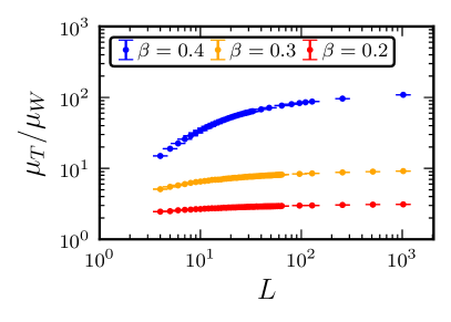
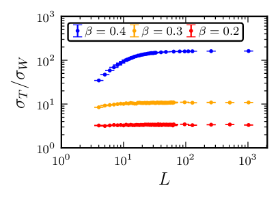
Figure 8: Monte Carlo estimates of $\mu_{T}/\mu_{W}$ (left) and $\sigma_{T}/\sigma_{W}$ (right) for the Ising heat-bath process with $d=2$ and $\beta<\beta_{\mathrm{c}}$ values as specified in the figure. Error bars corresponding to one standard error are shown.

Turning to the critical case, Fig. 9 shows the $L$ dependence of $\mu_{T}$ and $\sigma_{T}$ for $d=2$. The figure clearly suggests that both $\mu_{T}/L^{d}$ and $\sigma_{T}/L^{d}$ diverge like a power law in $L$, with the same exponent. A least squares analysis for $\mu_{T}$ produces a power-law exponent $2.168(4)$, while an analogous analysis for $\sigma_{T}$ produces an exponent

$$z_{T}=2.166(9).$$ (7.3)

The combination of the figure and the fits lends strong support to Part (ii) of Conjecture 7.1, that $\mu_{T}/\sigma_{T}$ approaches a constant as $L\to\infty$.

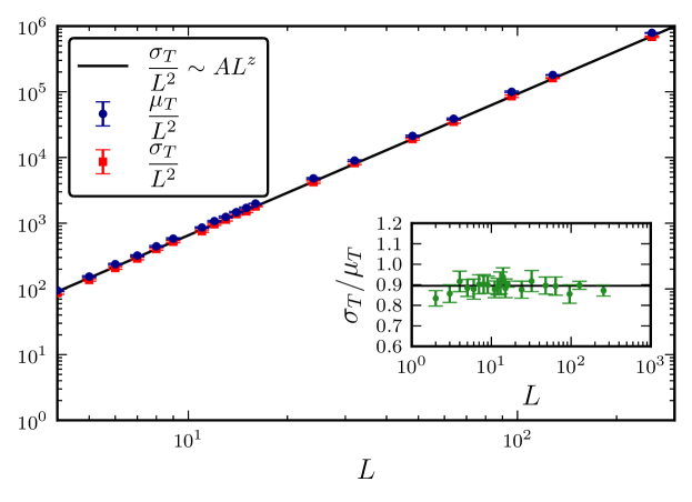
Figure 9: Monte Carlo estimates of $\mu_{T}/L^{d}$ and $\sigma_{T}/L^{d}$ for the critical Ising heat-bath process with $d=2$. The solid black line shows the curve $AL^{z}$, with the estimated values of $A$ and $z=2.166$. The inset shows the ratio $\sigma_{T}/\mu_{T}$. The solid line within the inset corresponds to the estimated asymptotic limit of $\sigma_{T}/\mu_{T}\rightarrow 0.895(8)$. Error bars corresponding to one standard error are shown.

7.4 Variance and relaxation time

We now turn attention to Part (iii) of Conjecture 7.1. We first consider the case $d=1$, where the relaxation time can be calculated explicitly. It was shown in (Nacu03, , Lemma 4) that if the transition matrix, $P$, of the Ising heat-bath process (on any graph) has a strictly increasing eigenfunction, then its eigenvalue is the second-largest eigenvalue, $\lambda_{2}$. The total magnetization $\mathcal{M}=\sum_{i=1}^{L}\omega_{i}$ is clearly strictly increasing. Moreover, on $\mathbb{Z}_{L}$ it is known (see e.g. the proof of Theorem 15.4 in LevinPeresWilmer09 ) that $\mathcal{M}$ is an eigenfunction of $P$ with eigenvalue

$$\lambda(\beta)=1-\frac{1-\tanh{(2\beta)}}{L}.$$ (7.4)

This immediately yields the following closed-form expression for the relaxation time on $\mathbb{Z}_{L}$

$$t_{\mathrm{rel}}(L)=\frac{L}{1-\tanh(2\beta)}.$$ (7.5)

Fig. 10 compares Monte Carlo estimates of $\sigma_{T}$ on $\mathbb{Z}_{L}$ with the exact expression for $t_{\mathrm{rel}}$ given in (7.5). The agreement is clearly excellent, over the entire range of $\beta$ considered, thus lending strong support to Part (iii) of Conjecture 7.1 in the case $d=1$.

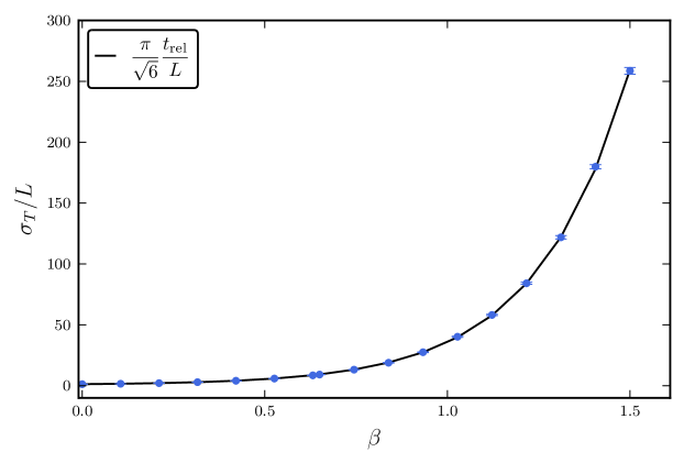
Figure 10: Monte Carlo estimates of $\sigma_{T}/L$ for the Ising heat-bath process on $\mathbb{Z}_{L}$ with $L=10^{4}$. The blue curve corresponds to the exact expression for $t_{\mathrm{rel}}/L$ given in (7.5). Error bars corresponding to one standard error are shown.

We now consider the case $d>1$, using analogous arguments to those presented in Section 3.3 in the FK setting. Let $(X_{t})_{t\in\mathbb{N}}$ be a stationary Ising heat-bath process, and define $(\mathcal{M}_{t})_{t\in\mathbb{N}}$ via $\mathcal{M}_{t}=\mathcal{M}(X_{t})$. Although Proposition A.1 is stated in the specific context of the FK heat-bath process, the positive association of the Ising measure (7.1) (see e.g. (FriedliVelenik16, , Theorem 3.31)) implies that the proof of Lemma A.2, and then also the proof of Proposition A.1, immediately extend to the Ising heat-bath process. It follows that, since the magnetization is strictly increasing, we have

$$\rho_{\mathcal{M}}(t)\sim Ce^{-t/t_{\exp}},\qquad t\to\infty$$ (7.6)

for some (parameter dependent) constant $C>0$. Assuming the validity of Part (iii) of Conjecture 7.1, it follows from (7.6) that

$$\ln\rho_{\mathcal{M}}(k\,\sigma_{T})\sim-C(\beta,d)\,k$$ (7.7)

as $k$ and $L$ tend to infinity, with $C(\beta,d)>0$, and with $C(\beta,d)=\pi/\sqrt{6}$ for all $\beta<\beta_{\mathrm{c}}$.

For a given time lag $t$, we estimated $\rho_{\mathcal{M}}(t)$ using the procedure described in Section 3.3 for the estimation of $\rho_{\mathcal{N}}(t)$ for the FK model. Fig. 11 shows the resulting estimates of $\rho_{\mathcal{M}}(k\,\sigma_{T})$ versus $k$ for $d=2$, in the high-temperature regime (left panel) and at criticality (right panel), for a variety of $L$ values. In both cases, the data collapse evident in the figure clearly supports the expectation (7.7), and therefore provides direct evidence to support the conjecture that $\sigma_{T}\sim C(\beta,d)\,t_{\mathrm{rel}}$. Moreover, in the high-temperature case, the collapse of the curves arising from distinct temperature values onto a single curve corresponding to $\exp(-k\pi/\sqrt{6})$, supports the claim that $C(\beta,d)=\pi/\sqrt{6}$ when $\beta<\beta_{\mathrm{c}}$.

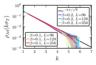
Figure 11: Monte Carlo estimates of $\ln\rho_{\mathcal{M}}(\sigma_{T}\,k)$ for the Ising heat-bath process with $d=2$ in high temperature (left) and at criticality (right). The enclosing filled regions correspond to one standard error.

$L$	$\sigma_{T}/t_{\exp}$
4	0.895(1)
5	0.894(3)
6	0.901(3)
7	0.897(3)
8	0.889(3)
9	0.898(4)
10	0.890(3)
11	0.893(3)
12	0.904(3)
13	0.893(3)
14	0.896(4)
15	0.894(3)

Table 4: Ratios of estimated $\sigma_{T}$ values to the estimated values of $t_{\exp}$ from NightingaleBloete96 , for the critical Ising heat-bath process when $d=2$. Error bars corresponding to one standard error are shown.

In the critical case, we have no explicit conjecture for the value of $C(\beta,d)$. However, using the critical $d=2$ values of $t_{\exp}$ reported in NightingaleBloete96 , we computed the ratios $\sigma_{T}/t_{\exp}$, which are reported in Table 4. The first observation to make is that, for the $L$ values considered, there appears to be extremely weak $L$ dependence; in fact, the size of any $L$ dependence appears to be smaller than our statistical errors. In particular, this gives direct, independent, support to the conjectured asymptotic proportionality of $\sigma_{T}$ and $t_{\exp}$. Furthermore, it suggests that we have $C(\beta_{\mathrm{c}},2)\approx 0.895$. It is interesting to note that this constant agrees, within error bars, with the constant of proportionality relating $\sigma_{T}$ to $\mu_{T}$, reported in Fig. 9, suggesting the possibility that $\mu_{T}\sim t_{\exp}$ at criticality, at least when $d=2$.

Finally, as yet further evidence to support Part (iii) of Conjecture 7.1 in the critical case, we note that the estimated value of the exponent (7.3), governing $\sigma_{T}$ at criticality for $d=2$, agrees, within error bars, with Grassberger’s Grassberger95 estimate for the dynamic exponent $z_{\exp}=2.172(6)$.

7.5 Limit law

Fig. 12(a) plots the empirical distribution of the standardized coupling time $S:=(T-\mu_{T})/\sigma_{T}$ for a high-temperature Ising heat-bath process with $d=2$ and $L=1024$. The agreement with the Gumbel distribution (2.19) clearly supports Part (iv) of Conjecture 7.1 in the case $\beta<\beta_{\mathrm{c}}$. Fig. 12(b) shows the critical case, again with $d=2$. The data collapse of the $L=128$ and $L=256$ curves strongly supports the claim that $S$ converges in distribution to a non-degenerate limit, thus supporting Part (iv) of Conjecture 7.1 in the case $\beta=\beta_{\mathrm{c}}$. However, it is clear that this limiting distribution is not $G(x)$.

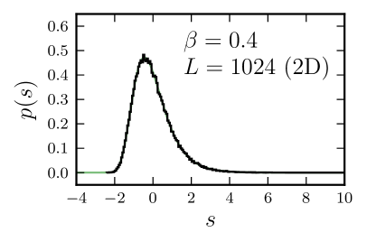
(a)

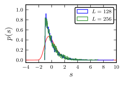
(b)

Figure 12: Histogram of $S$ at high temperature (left) and criticality (right), with parameters as specified in the figure. Here $p(s)$ denotes the probability density function of $S$. For comparison, the solid green line shows the probability density function corresponding to (2.19).

Appendix A Autocorrelation functions of strictly increasing observables

Let $P$ denote the transition matrix of the FK heat-bath process on a finite graph $G=(V,E)$ with parameters $p\in(0,1)$ and $q\geq 1$, and let $k=2^{|E|}$. To avoid trivialities, we assume $|E|>1$. We regard elements of $\mathbb{R}^{k}$ as functions from $2^{E}$ to $\mathbb{R}$, and we endow $\mathbb{R}^{k}$ with the inner product $\langle\cdot,\cdot\rangle$ defined by

$$\langle g,h\rangle:=\sum_{A\subseteq E}g(A)\,h(A)\,\phi(A).$$

Denote the eigenvalues of $P$ by $1=\lambda_{1}>\lambda_{2}\geq\ldots\geq\lambda_{k}$. As mentioned in Section 2.2, general results for heat-bath chains DyerGreenhillUllrich14 imply that all $\lambda_{i}$ are non-negative. Let $\{\psi_{i}\}_{i=1}^{k}$ be an orthonormal basis for $\mathbb{R}^{k}$ such that $\psi_{i}$ is an eigenfunction of $P$ corresponding to $\lambda_{i}$. The Perron-Frobenius theorem implies that the eigenspace of $\lambda_{1}$ is one-dimensional, and that we can take $\psi_{1}(A)=1$ for all $A\subseteq E$. Let $W$ denote the eigenspace of $\lambda_{2}$. For $g\in\mathbb{R}^{k}$, we let $g_{W}$ denote its projection onto $W$.

We say $g\in\mathbb{R}^{k}$ is increasing if $A\subset B$ implies $g(A)\leq g(B)$, and strictly increasing if $A\subset B$ implies $g(A)<g(B)$.

Proposition A.1.

Let $(X_{t})_{t\in\mathbb{N}}$ be a stationary FK heat-bath process, and for $g\in\mathbb{R}^{k}$ define $(g_{t})_{t\in\mathbb{N}}$ via $g_{t}:=g(X_{t})$. If $g$ is strictly increasing, then its autocorrelation function satisfies

$$\rho_{g}(t):=\frac{\operatorname{cov}(g_{0},g_{t})}{\operatorname{var}(g_{0})}\sim Ce^{-t/t_{\exp}},\qquad t\to\infty,$$

for constant $C>0$.

Proof.

Let $\Pi$ denote the projection matrix onto the space of constant functions. General arguments (see e.g. Sokal97 or (MadrasSlade96, , Chapter 9)) imply

$$\operatorname{cov}(g_{0},g_{t})=\langle g,(P^{t}-\Pi)g\rangle=\sum_{l=2}^{k}\langle g,\psi_{l}\rangle^{2}\lambda_{l}^{t}=\|g_{W}\|^{2}\lambda_{2}^{t}\,+\,\sum_{l=\dim(W)+2}^{k}\langle g,\psi_{l}\rangle^{2}\lambda_{l}^{t}.$$

Since $g$ is strictly increasing, Lemma A.2 implies that $\|g_{W}\|^{2}>0$, and therefore

$$\operatorname{cov}(g_{0},g_{t})\sim\|g_{W}\|^{2}e^{-t/t_{\exp}},\qquad t\to\infty.$$

It follows that

$$\rho_{g}(t)\sim\frac{\|g_{W}\|^{2}}{\operatorname{var}(g)}e^{-t/t_{\exp}},\qquad t\to\infty.$$

∎

Lemma A.2.

If $g$ is strictly increasing, then its projection onto $W$ is non-zero.

Proof.

Lemma A.3 implies there exists $\psi\in W$ which is non-zero and increasing. Positive association (see e.g. (Grimmett06, , Theorem 3.8 (b))) then implies that for any other increasing $g$ we have

$$\langle g,\psi\rangle\geq\mathbb{E}(g)\,\mathbb{E}(\psi)=0,$$ (A.1)

since $\mathbb{E}(\psi)=\langle\psi_{1},\psi\rangle=0$. In particular, suppose that $g$ is strictly increasing. Choosing $\alpha>0$ so that

$$g(B)-g(A)>\alpha[\psi(B)-\psi(A)],\qquad\text{ for all }A\subset B\subseteq E,$$

implies that $g-\alpha\psi$ is also strictly increasing. Applying (A.1) to $g-\alpha\psi$ then yields

$$\langle g-\alpha\psi,\psi\rangle\geq 0.$$

Rearranging, and using the fact that $\psi$ is non-zero then implies

$$\langle g,\psi\rangle\geq\alpha\langle\psi,\psi\rangle>0.$$

Therefore, $g$ has a non-zero projection onto $\psi\in W$, and the stated result follows. ∎

The following lemma is the natural analogue, in the FK setting, of the result (Nacu03, , Lemma 3) established for the Ising heat-bath process.

Lemma A.3.

There exists $\psi\in W$ which is non-zero and increasing.

Proof.

Let $g=\psi_{2}+C(\mathcal{N}-\mathbb{E}(\mathcal{N}))$, where $\mathcal{N}\in\mathbb{R}^{k}$ is defined so that $\mathcal{N}(A)=|A|$ for each $A\subseteq E$, and $C>0$ is a constant. We have

$$g=[1+C\langle\mathcal{N},\psi_{2}\rangle]\psi_{2}+C\sum_{j=3}^{k}\langle\mathcal{N},\psi_{j}\rangle\psi_{j}.$$

If $\langle\mathcal{N},\psi_{2}\rangle=0$, then $g$ has a non-zero projection onto $\psi_{2}$, for any choice of $C>0$. If $\langle\mathcal{N},\psi_{2}\rangle\neq 0$, then choosing $C>|\langle\mathcal{N},\psi_{2}\rangle|^{-1}$ suffices to guarantee that $g$ again has a non-zero projection onto $\psi_{2}$. In either case, assume $C$ is so chosen. It follows that $g_{W}$ is non-zero.

If $A\subset B$, then

$$g(B)-g(A)=\psi_{2}(B)-\psi_{2}(A)+C[\mathcal{N}(B)-\mathcal{N}(A)]\geq\min_{A\subset B\subseteq E}[\psi_{2}(B)-\psi_{2}(A)]+C.$$

Therefore, by choosing $C>\left|\min\limits_{A\subset B\subseteq E}[\psi_{2}(B)-\psi_{2}(A)]\right|$ we guarantee that $g$ is increasing. Lemma A.4 then implies that $g_{W}$ is increasing. Therefore, $\psi=g_{W}$ is an increasing, non-zero element of $W$. ∎

Lemma A.4.

If $g$ is increasing and has zero-mean, then its projection onto $W$ is also increasing.

Proof.

Let $g\in\mathbb{R}^{k}$ be any increasing observable with mean zero, and let $t\in\mathbb{N}^{+}$. Since Lemma A.6 implies $\lambda_{2}>0$, we can write

$$\frac{P^{t}g}{\lambda_{2}^{t}}=g_{W}+\sum_{l=\dim(W)+2}^{k}\langle g,\psi_{l}\rangle\psi_{l}\,\left(\frac{\lambda_{l}}{\lambda_{2}}\right)^{t}.$$

It follows that

$$\lim_{t\to\infty}\frac{P^{t}g}{\lambda_{2}^{t}}=g_{W}.$$ (A.2)

Now, for any given $t\geq 1$, Lemma A.5 implies that $P^{t}g(A)$ is an increasing function of $A$, and so $\lambda_{2}^{-t}P^{t}g(A)$ is also an increasing function of $A$. It then follows, as an elementary consequence of (A.2), that $g_{W}$ is also increasing. We have therefore established that if $g$ is an increasing zero-mean function, then its projection $g_{W}$ is also increasing. ∎

Lemma A.5.

If $g\in\mathbb{R}^{k}$ is increasing, then $P^{t}g$ is also increasing, for every $t\geq 1$.

Proof.

Let $(f,\mathcal{E},U)$ be the random mapping representation for $P$ given in Section 2.1; see (2.3). Let $A_{1}\subset A_{2}\subseteq E$, and let $B_{i}=f(A_{i},\mathcal{E},U)$ for $i=1,2$. Clearly, $(B_{1},B_{2})$ is a coupling of the distributions $P(A_{1},\cdot)$ and $P(A_{2},\cdot)$, and the monotonicity of $f$ implies $B_{1}\subseteq B_{2}$. Strassen’s theorem (see e.g. (Grimmett10, , Theorem 4.2)) then implies that

$$\mathbb{E}_{P(A_{1},\cdot)}(g)\leq\mathbb{E}_{P(A_{2},\cdot)}(g)$$

for any increasing $g\in\mathbb{R}^{k}$. It follows that

$$(Pg)(A_{1})=\sum_{B\subseteq E}P(A_{1},B)g(B)=\mathbb{E}_{P(A_{1},\cdot)}(g)\leq\mathbb{E}_{P(A_{2},\cdot)}(g)=\sum_{B\subseteq E}P(A_{2},B)g(B)=(Pg)(A_{2}).$$

Since this holds for any $A_{1}\subset A_{2}\subseteq E$, it follows that $Pg$ is increasing. It then follows by a simple induction that $P^{t}g$ is increasing for any $t\geq 1$. ∎

Lemma A.6.

The second-largest eigenvalue of $P$ is positive.

Proof.

Since $P$ is reversible and irreducible we have the spectral decomposition (see e.g. (LevinPeresWilmer09, , Lemma 12.2))

$$\frac{P(A,B)}{\phi(B)}=1+\sum_{j=2}^{k}\psi_{i}(A)\psi_{i}(B)\lambda_{i}.$$

Since $\lambda_{2}\geq\lambda_{j}\geq 0$ for all $j>2$, it follows that if $\lambda_{2}=0$, then $P(A,B)=\phi(B)$ for all $A,B\subseteq E$. But since, by assumption, we have $|E|>1$, we can choose $A,B\subseteq E$ with $|A\triangle B|>1$, where $\triangle$ denotes symmetric difference, and (2.2) then implies

$$P(A,B)=0\neq\phi(B).$$

We have therefore reached a contradiction, and we conclude that $\lambda_{2}>0$. ∎

Appendix B Coupon Collecting

Let $n\in\mathbb{N}^{+}$, and let $C_{1},C_{2},\ldots$ be an iid sequence of uniformly random elements of $[n]:=\{1,2,\ldots,n\}$. For $t\in\mathbb{N}^{+}$, we think of $C_{t}$ as the coupon collected at time $t$. For $i\in[n]$, let $D_{i}\in[n]$ denote the $i$th distinct type of coupon collected; i.e. the $i$th distinct element of the sequence $C_{1},C_{2},\ldots$. Let $S_{i}(t):=\#\{s\leq t:C_{s}=D_{i}\}$, the number of copies of $D_{i}$ collected by time $t$. Define $R_{t}:=\{c\in[n]:C_{s}=c\textrm{ for some }s\leq t\}$, the set of distinct coupon types collected up to time $t$. For any $1\leq k\leq n$, let $W_{k}=\inf\{t\in\mathbb{N}^{+}:|R_{t}|=k\}$, and note that $W_{k}$ is simply the hitting time of $D_{k}$. The coupon collector’s time is then defined as $W:=W_{n}$.

For each $c\in[n]$, define

$$H(c)=\sup\{t\leq W:C_{t}=c\}.$$

We refer to the time $H(c)$ as the last visit to $c$. Let $(H_{i})_{i=1}^{n}$ denote the sequence of the $H(c)$, arranged in increasing order. In particular, $H_{1}$ is the first time that a last visit occurs.

Lemma B.1.

There exists $\varphi>0$ such that $\mathbb{P}(|R_{H_{1}}|\leq\left\lfloor\ln n\right\rfloor)=O(n^{-\varphi})$.

Proof.

Inserting $a_{n}=\lfloor\ln(n)\rfloor$ and $c_{n}=\lfloor\ln(n)/4\rfloor$ into Lemma B.2 and applying the union bound, implies

$$\mathbb{P}\left(\bigcup_{i=1}^{a_{n}}\left\{S_{i}(W)\leq c_{n}\right\}\right) \leq\ln(n)\exp\left(-\frac{1}{2}\ln(n-a_{n})+\frac{\ln(n)}{4}+1\right)$$

$$=e\,\ln(n)\exp\left(-\frac{1}{4}\ln(n)-\frac{1}{2}\ln\left(1-\frac{a_{n}}{n}\right)\right)$$

$$=\frac{e}{\sqrt{1-\lfloor\ln(n)\rfloor/n}}\,\ln(n)\,n^{-1/4}.$$

Therefore, for any $0<\rho<1/4$, we have

$$\mathbb{P}\left(\bigcup_{i=1}^{a_{n}}\left\{S_{i}(W)\leq c_{n}\right\}\right)=O(n^{-\rho}),\qquad n\to\infty.$$

It follows that,

$$\mathbb{P}(|R_{H_{1}}|\leq a_{n})=\mathbb{P}\left(|R_{H_{1}}|\leq a_{n},\bigcap_{i=1}^{a_{n}}\{S_{i}(W)>c_{n}\}\right)+O(n^{-\rho})$$ (B.1)

Let $I:=\inf\{t\in\mathbb{N}^{+}:S_{i}(t)=c_{n}\textrm{ for some }i\in[n]\}$, the first time that there exists a coupon type for which exactly $c_{n}$ copies have been collected, and define the random variable $K\in[n]$ via $C_{H_{1}}=D_{K}$. If $|R_{H_{1}}|\leq a_{n}$, then $1\leq K\leq a_{n}$. Therefore, observing that $S_{K}(W)=S_{K}(H_{1})$, we find

$$\begin{split}\mathbb{P}\left(|R_{H_{1}}|\leq a_{n},\bigcap_{i=1}^{a_{n}}\{S_{i}(W)>c_{n}\}\right)&\leq\mathbb{P}(|R_{H_{1}}|\leq a_{n},S_{K}(W)>c_{n})\\ &=\mathbb{P}(|R_{H_{1}}|\leq a_{n},S_{K}(H_{1})>c_{n})\\ &\leq\mathbb{P}(|R_{I}|\leq a_{n})\end{split}$$ (B.2)

since if $|R_{H_{1}}|\leq a_{n}$ and $S_{K}(H_{1})>c_{n}$ then $|R_{I}|\leq a_{n}$. Combining (B.1) and (B.2) then implies

$$\mathbb{P}(|R_{H_{1}}|\leq a_{n})\leq\mathbb{P}(|R_{I}|\leq a_{n})+O(n^{-\rho}).$$

However, Lemma B.3 implies that there exists $\delta>0$ such that $\mathbb{P}(|R_{I}|\leq a_{n})=O(n^{-\delta})$. We therefore conclude that, if $\varphi=\min\{\rho,\delta\}$, then

$$\mathbb{P}(|R_{H_{1}}|\leq\left\lfloor\ln n\right\rfloor)=O(n^{-\varphi}).$$

∎

Lemma B.2.

Let $(a_{n})_{n\in\mathbb{N}^{+}}$ and $(c_{n})_{n\in\mathbb{N}^{+}}$ be any two sequences of natural numbers. For $n\in\mathbb{N}^{+}$, if $a_{n}<n$ then for each $1\leq i\leq a_{n}$ we have

$$\mathbb{P}\left(S_{i}(W)\leq c_{n}\right)\leq\exp\left(-\ln(\sqrt{n-a_{n}})+c_{n}+1\right).$$

Proof.

Fix $n\in\mathbb{N}^{+}$ and $1\leq i\leq a_{n}$, and assume $a_{n}<n$. Adopting the convention $W_{0}=0$, for $0\leq k\leq n-1$ we define

$$Y_{i}(k):=\sum_{j=W_{k}+1}^{W_{k+1}-1}\mathbf{1}_{\{C_{j}=D_{i}\}}.$$

Since $Y_{i}(k)=0$ for all $k<i$, and $C_{W_{k}}=D_{i}$ iff $k=i$, we then have

$$S_{i}(W)=1+\sum_{k=i}^{n-1}Y_{i}(k).$$

And since the random variables $Y_{i}(k)$ are independent, for any $\theta<0$, we have

$$\begin{split}\mathbb{P}\left(S_{i}(W)\leq c_{n}\right)&\leq\mathbb{P}\left(\sum_{k=a_{n}}^{n-1}Y_{i}(k)\leq c_{n}\right)\\ &=\mathbb{P}\left(\exp\left[\theta\sum_{k=a_{n}}^{n-1}Y_{i}(k)\right]\geq e^{\theta c_{n}}\right)\\ &\leq\exp\left(-\theta c_{n}+\sum_{k=a_{n}}^{n-1}\ln\mathbb{E}[e^{\theta Y_{i}(k)}]\right),\end{split}$$ (B.3)

where the final step follows from Markov’s inequality.

The moment generating function of $Y_{i}(k)$ can be calculated explicitly. Let $i\leq k\leq n-1$. Given $W_{k}$ and $W_{k+1}$, the random variable $Y_{i}(k)$ has binomial distribution with $W_{k+1}-W_{k}-1$ trials and success probability $1/k$, which implies

$$\mathbb{E}(e^{\theta Y_{i}(k)}) =\mathbb{E}(\mathbb{E}[e^{\theta Y_{i}(k)}|W_{k},W_{k+1}])$$

$$=\mathbb{E}\left[\left(\frac{e^{\theta}}{k}+1-\frac{1}{k}\right)^{W_{k+1}-W_{k}-1}\right].$$

But since $W_{k+1}-W_{k}$ has geometric distribution with parameter $1-k/n$, this becomes

$$\mathbb{E}(e^{\theta Y_{i}(k)})=\frac{n-k}{n-k+1-e^{\theta}}.$$

Therefore, setting $\lambda=1-e^{\theta}$ and $b_{n}=n-a_{n}$, it follows from the fact that $\ln(1+\lambda/k)$ is a decreasing function of $k$ that

$$\begin{split}-\sum_{k=a_{n}}^{n-1}\ln\mathbb{E}(e^{\theta Y_{i}(k)})&=\sum_{k=1}^{b_{n}}\ln\left(1+\frac{\lambda}{k}\right)\\ &\geq\int_{1}^{b_{n}}\ln\left(1+\frac{\lambda}{x}\right)\mathrm{d}\,x\\ &=\lambda\ln(b_{n})+(b_{n}+\lambda)\ln(1+\lambda/b_{n})-(1+\lambda)\ln(1+\lambda)\\ &\geq\lambda\ln(b_{n})+\lambda-(1+\lambda)\ln(1+\lambda)\\ &\geq\lambda\ln(b_{n})-1\end{split}$$ (B.4)

where, in the penultimate step, we used the fact that $\ln(1+x)\geq x/(1+x)$ holds for all $x>-1$, and in the last step we used the fact that $(1+\lambda)-(1+\lambda)\ln(1+\lambda)>0$ for any $\lambda\in(0,1)$. Combining (B.3) and (B.4), we conclude that for all $\lambda\in(0,1)$ we have

$$\mathbb{P}\left(S_{i}(W)\leq c_{n}\right)\leq\exp\left[-\lambda\ln(n-a_{n})-\ln(1-\lambda)c_{n}+1)\right].$$

Choosing $\lambda=1/2$ yields the stated result. ∎

Lemma B.3.

Fix $c\in(0,1)$, and define sequences $(a_{n})_{n\in\mathbb{N}^{+}}$ and $(c_{n})_{n\in\mathbb{N}^{+}}$ such that $a_{n}=\lfloor\ln(n)\rfloor$ and $c_{n}=\lfloor c\ln(n)\rfloor$. Let

$$I:=\inf\{t\in\mathbb{N}^{+}:S_{i}(t)=c_{n}\textrm{ for some }i\in[n]\},$$

the first time that there exists a coupon type for which exactly $c_{n}$ copies have been collected. Then there exists $\delta>0$ such that

$$\mathbb{P}(|R_{I}|\leq a_{n})=O(n^{-\delta}),\qquad n\to\infty.$$

Proof.

We assume, in all that follows, that $n$ is sufficiently large that $c_{n}>1$. For $k\in[n]$, let

$$I_{k}=\inf\{t\in\mathbb{N}^{+}:S_{k}(t)=c_{n}\}$$

be the first time that $c_{n}$ copies of coupon type $D_{k}$ have been collected. For any sequence of natural numbers $(b_{n})_{n\in\mathbb{N}^{+}}$, we have

$$\begin{split}\mathbb{P}(|R_{I_{k}}|\leq a_{n})&=\mathbb{P}(|R_{I_{k}}|\leq a_{n},I_{k}\leq b_{n})+\mathbb{P}(|R_{I_{k}}|\leq a_{n},I_{k}>b_{n})\\ &\leq\mathbb{P}(I_{k}\leq b_{n})+\mathbb{P}(|R_{I_{k}}|\leq a_{n},I_{k}>b_{n})\\ &\leq\mathbb{P}(I_{k}\leq b_{n})+\mathbb{P}(W_{a_{n}+1}>b_{n}),\end{split}$$ (B.5)

where the last inequality follows by observing that if $|R_{I_{k}}|\leq a_{n}$ and $I_{k}>b_{n}$, then $W_{a_{n}+1}>b_{n}$.

To find an upper bound for $\mathbb{P}(I_{k}\leq b_{n})$, note that, for any $s\geq 1$, the random time between the $s$th and $(s+1)$th arrival of coupon type $D_{k}$ is a geometric random variable with success probability $1/n$. It follows that $\Delta_{k}:=I_{k}-W_{k}$ is a sum of $c_{n}-1$ independent geometric random variables, each with success probability $1/n$. Lemma B.4 therefore implies that for any $0<\lambda<1$,

$$\mathbb{P}(\Delta_{k}\leq\lambda n(c_{n}-1))\leq e^{-f(\lambda)c_{n}+f(\lambda)}$$

where $f(\lambda)>0$. But from the trivial lower bound $W_{k}\geq 1$, it follows that $\Delta_{k}\leq I_{k}-1$. Therefore, for any $b_{n}\leq\lambda n(c_{n}-1)+1$, we have

$$\mathbb{P}(I_{k}\leq b_{n})\leq\mathbb{P}(I_{k}\leq\lambda n(c_{n}-1)+1)\leq\mathbb{P}(\Delta_{k}\leq\lambda n(c_{n}-1))\leq e^{-f(\lambda)c_{n}+f(\lambda)}.$$ (B.6)

To find an upper bound for $\mathbb{P}(W_{a_{n}+1}>b_{n})$, we begin with the observation that, with the convention $W_{0}=0$, we have

$$W_{a_{n}+1}=\sum_{i=0}^{a_{n}}(W_{i+1}-W_{i}).$$

For $0\leq i\leq a_{n}$, the random variables $W_{i+1}-W_{i}$ are independent, and distributed according to a geometric distribution with success probability $1-i/n$. Therefore, Lemma B.4 implies that for any $\zeta>1$

$$\mathbb{P}(W_{a_{n}+1}\geq\zeta\,\mathbb{E}[W_{a_{n}+1}])\leq e^{-f(\zeta)(1-a_{n}/n)\mathbb{E}(W_{a_{n}+1})}$$

with $f(\zeta)>0$. But explicit calculation shows that

$$\mathbb{E}(W_{a_{n}+1})=n(H_{n}-H_{n-a_{n}-1})\sim a_{n},\qquad n\to\infty,$$

where $H_{i}$ is the $i$th harmonic number, and the asymptotic result follows from $H_{n}\sim\ln(n)$ and the fact that $a_{n}=o(n)$. It follows that for any choice of $b_{n}\geq\zeta\,\mathbb{E}(W_{a_{n}+1})$ and $\alpha\in(0,f(\zeta))$, for sufficiently large $n$, we have

$$\mathbb{P}(W_{a_{n}+1}\geq b_{n})\leq e^{-\alpha\,a_{n}}.$$ (B.7)

Any choice of $b_{n}$ satisfying $\zeta\,\mathbb{E}(W_{a_{n}+1})\leq b_{n}\leq\lambda n(c_{n}-1)+1$, for sufficiently large $n$, suffices to ensure (B.6) and (B.7) hold simultaneously. It therefore suffices to set $b_{n}=n$. For simplicity, $\lambda\in(0,1)$ and $\zeta>1$ can be chosen so that $f(\lambda)=1=f(\zeta)$. Combining (B.5), (B.6) and (B.7) then implies that for any $\alpha<1$ we have

$$\mathbb{P}(|R_{I_{k}}|\leq a_{n})\leq e^{-c_{n}+1}+e^{-\alpha\,a_{n}}$$

for sufficiently large $n$.

Finally, since $|R_{I}|\leq a_{n}$ implies $|R_{I_{k}}|\leq a_{n}$ for some $1\leq k\leq a_{n}$, it follows from the union bound that, for sufficiently large $n$,

$$\mathbb{P}(|R_{I}|\leq a_{n})\leq\mathbb{P}\left(\bigcup_{k=1}^{a_{n}}\{|R_{I_{k}}|\leq a_{n}\}\right)\leq\sum_{k=1}^{a_{n}}\mathbb{P}(|R_{I_{k}}|\leq a_{n}) \leq a_{n}\,e^{-c_{n}+1}+a_{n}\,e^{-\alpha\,a_{n}}$$

$$\leq e^{2}\,\ln(n)\,n^{-c}+e^{\alpha}\,\ln(n)\,n^{-\alpha}.$$

Since $c,\alpha>0$, we can choose $0<\delta<\min\{c,\alpha\}$, and we obtain $\mathbb{P}(|R_{I}|\leq a_{n})=O(n^{-\delta})$. ∎

Lemma B.4.

Let $X_{1},X_{2},\ldots,X_{n}$ be independent random variables, such that $X_{i}$ has geometric distribution with success probability $p_{i}$, and let $X=\sum_{i=1}^{n}X_{i}$. Then

$$\mathbb{P}(X\leq\lambda\mu) \leq e^{-p_{\ast}\mu f(\lambda)},\qquad\forall\,\lambda\leq 1,$$

$$\mathbb{P}(X\geq\zeta\mu) \leq e^{-p_{\ast}\mu f(\zeta)},\qquad\forall\,\zeta\geq 1,$$

where $\mu=\mathbb{E}(X)=\sum_{i=1}^{n}1/p_{i}$, $p_{\ast}=\min_{i\in[n]}p_{i}$ and $f(x)=x-1-\ln(x)$.

Proof.

These results can be established, in the standard way, by applying Markov’s inequality to $\mathbb{E}(e^{tX})$, and using the explicit form for $\mathbb{E}(e^{tX_{i}})$; see e.g. Janson14 . ∎

References

- (1) Aizenman, M., Duminil-Copin, H., Sidoravicius, V.: Random Currents and Continuity of Ising Model’s Spontaneous Magnetization. Communications in Mathematical Physics 334, 719–742 (2015)
- (2) Baxter, R.J.: Solvable eight-vertex model on an arbitrary planar lattice. Philosophical Transactions of the Royal Society A 289, 315–346 (1978)
- (3) Beffara, V., Duminil-Copin, H.: The self-dual point of the two-dimensional random-cluster model is critical for q 1. Probability Theory and Related Fields 153, 511–542 (2012)
- (4) Billingsley, P.: Probability and Measure, 3rd ed. (Wiley Series in Probability and Statistics), 3 edn. Wiley, New York (1994)
- (5) Cesi, F., Guadagni, G., Martinelli, F., Schonmann, R.H.: On the Two-Dimensional Stochastic Ising Model in the Phase Coexistence Region Near the Critical Point. Journal of Statistical Physics 85, 55–102 (1996)
- (6) Chayes, L., Machta, J.: Graphical representations and cluster algorithms II. Physica A 254, 477–516 (1998)
- (7) Chow, Y.S., Teicher, H.: Probability Theory: Independence, Interchangeability, Martingales. Springer, New York (1978)
- (8) Deng, Y., Blöte, H.: Simultaneous analysis of several models in the three-dimensional Ising universality class. Physical Review E 68, 036,125 (2003)
- (9) Deng, Y., Garoni, T., Machta, J., Ossola, G., Polin, M., Sokal, A.: Critical Behavior of the Chayes–Machta–Swendsen–Wang Dynamics. Physical Review Letters 99, 055,701 (2007)
- (10) Deng, Y., Garoni, T.M., Sokal, A.D.: Critical speeding-up in the local dynamics of the random-cluster model. Physical Review Letters 98, 230,602 (2007)
- (11) Duminil-Copin, H., Gagnebin, M., Harel, M., Manolescu, I., Tassion, V.: Discontinuity of the phase transition for the planar random-cluster and Potts models with . arXiv:1611.09877 (2016)
- (12) Duminil-Copin, H., Sidoravicius, V., Tassion, V.: Continuity of the phase transition for planar random-cluster and Potts models with . arXiv:1602.05677 (2016)
- (13) Dyer, M., Greenhill, C., Ullrich, M.: Structure and eigenvalues of heat-bath Markov chains. Linear Algebra and its Applications 454, 57–71 (2014)
- (14) Elci, E.: Algorithmic and geometric aspects of the random-cluster model. Ph.D. thesis (2015)
- (15) Elçi, E.M., Weigel, M.: Efficient simulation of the random-cluster model. Physical Review E 88, 033,303 (2013)
- (16) Elçi, E.M., Weigel, M.: Dynamic connectivity algorithms for Monte Carlo simulations of the random-cluster model. Journal of Physics: Conference Series 510, 012,013–10 (2014)
- (17) Erdos, P., Renyi, A.: On a classical problem of probability theory. Publ. Math. Inst. Hung. Acad. Sci., Ser. A 6, 215–219 (1961)
- (18) Feller, W.: An Introduction to Probability Theory and Its Applications, vol. 1, 3 edn. John Wiley & Sons Inc, New York (1968)
- (19) Friedli, S., Velenik, Y.: Statistical Mechanics of Lattice Systems. A Concrete Mathematical Introduction. Cambridge University Press, Cambridge (2016)
- (20) Gheissari, R., Lubetzky, E.: Mixing Times Of Critical 2D Potts Models. arXiv:1607.02182 (2016)
- (21) Gliozzi, F.: Simulation of Potts models with real q and no critical slowing down. Physical Review E 66, 016,115 (2002)
- (22) Graham, R.L., Knuth, D.E., Patashnik, O.: CONCRETE MATHEMATICS, 2 edn. A Foundation for Computer Science. Addisen-Wesley Publishing Company (1994)
- (23) Grassberger, P.: Damage spreading and critical exponents for “model A” Ising dynamics. Physica A 214, 547–559 (1995)
- (24) Grimmett, G.: The Random-Cluster Model. Springer, New York (2006)
- (25) Grimmett, G.: Probability on Graphs. Cambridge University Press, Cambridge (2010)
- (26) Guo, H., Jerrum, M.: Random cluster dynamics for the Ising model is rapidly mixing. arXiv:1605.00139 pp. 1–15 (2016)
- (27) Häggström, O.: Finite Markov Chains and Algorithmic Applications. Cambridge University Press, Cambridge (2003)
- (28) Hartmann, A.: Calculation of Partition Functions by Measuring Component Distributions. Physical Review Letters 94, 050,601 (2005)
- (29) Holm, J., de Lichtenberg, K., Thorup, M.: Poly-logarithmic deterministic fully-dynamic algorithms for connectivity, minimum spanning tree, 2-edge, and biconnectivity. Journal of the ACM (JACM) 48, 723–760 (2001)
- (30) Jaeger, F., Vertigan, D.L., Welsh, D.J.A.: On the computational complexity of the Jones and Tutte polynomials. Mathematical Proceedings of the Cambridge Philosophical Society 108, 35–53 (1990)
- (31) Janson, S.: Tail bounds for sums of geometric and exponential random variables (2014). URL http://www2.math.uu.se/~svante/papers/sjN14.pdf
- (32) Jerrum, M.: Mathematical Foundations of the Markov Chain Monte Carlo Method. In: Probabilistic Methods for Algorithmic Discrete Mathematics, pp. 116–165. Springer, New York (1998)
- (33) Laanait, L., Messager, A., Miracle-Solé, S., Ruiz, J., Shlosman, S.: Interfaces in the Potts model I: Pirogov-Sinai theory of the Fortuin-Kasteleyn representation. Communications in Mathematical Physics 140(1), 81–91 (1991)
- (34) Leadbetter, M.R., Lindgren, G., Rootzen, H.: Extremes and related properties of random sequences and processes. Springer, New York (1983)
- (35) Levin, D.A., Peres, Y., Wilmer, E.L.: Markov Chains and Mixing Times. American Mathematical Society, Providence (2009)
- (36) Madras, N., Slade, G.: The Self-Avoiding Walk. Birkhauser, Boston (1996)
- (37) McCoy, B.M., Wu, T.T.: The Two-Dimensional Ising Model. Harvard University Press, Cambridge (1973)
- (38) Mitzenmacher, M., Upfal, E.: Probability and Computing. Randomized Algorithms and Probabilistic Analysis. Cambridge University Press, Cambridge (2005)
- (39) Nacu, S.: Glauber dynamics on the cycle is monotone. Probability Theory and Related Fields 127, 177–185 (2003)
- (40) Nienhuis, B.: Critical behavior of two-dimensional spin models and charge asymmetry in the Coulomb gas. Journal of Statistical Physics 34, 731–761 (1984)
- (41) Nightingale, M.P., Bloete, H.W.J.: Dynamic Exponent of the Two-Dimensional Ising Model and Monte Carlo Computation of the Subdominant Eigenvalue of the Stochastic Matrix . Physical Review Letters 76, 4548–4551 (1996)
- (42) Posfai, A.: Approximation Theorems Related to the Coupon Collector’s Problem . Ph.D. thesis (2010)
- (43) Propp, J., Wilson, D.: Exact sampling with coupled Markov chains and applications to statistical mechanics. Random Structures and Algorithms 9, 223–252 (1996)
- (44) Sinclair, A.B., Alistair, Sinclair, A.: Random-Cluster Dynamics in . In: Twenty-Seventh Annual ACM-SIAM Symposium on Discrete Algorithms, pp. 498–513 (2016)
- (45) Sokal, A.D.: Monte Carlo Methods in Statistical Mechanics: Foundations and New Algorithms. In: C. DeWitt-Morette, P. Cartier, A. Folacci (eds.) Functional Integration: Basics and Applications (1996 Cargèse summer school), pp. 131–192. Plenum, New York (1997)
- (46) Sweeny, M.: Monte Carlo study of weighted percolation clusters relevant to the Potts models. Physical Review B 27, 4445–4455 (1983)
- (47) Swendsen, R.H., Wang, J.S.: Nonuniversal critical dynamics in Monte Carlo simulations. Physical Review Letters 58, 86–88 (1987)
- (48) Wang, J.S., Kozan, O., Swendsen, R.: Sweeny and Gliozzi dynamics for simulations of Potts models in the Fortuin-Kasteleyn representation. Physical Review E 66 (2002)
- (49) Welsh, D.J.A.: Complexity: Knots, Colourings and Counting, London Mathematical Society Lecture Note Series, vol. 186. Cambridge University Press (1993)
- (50) Youjin Deng, Timothy M. Garoni, Alan Sokal and ZongzhengZhou: Dynamic critical behavior of the Chayes-Machta random-cluster algorithm II: Three-dimensions. In preparation
- (51) Young, P.: Everything you wanted to know about Data Analysis and Fitting but were afraid to ask . Springer, New York (2015)