Shadow wave function with a symmetric kernel

Abstract

A shadow wave function with an explicit symmetric kernel is introduced. As a consequence the atoms exchange in the system is enhanced. Basic properties of this class of trial functions are kept and quantities it can describe are easily estimated. The effectiveness of this approach is analized by computing properties of interest in a system formed from ⁴He atoms.

I Introduction

Quantum matter that shows effects at the macroscopic level has attracted attention of physicists for many decades. One of the most studied systems presenting this behavior is formed from helium atoms. The richness of phenomena observed in both the liquid and solid phases of helium justify an interest that persists until today.

Variational theories are important tools in the investigation of quantum many-body systems. They are able to give physical insight in the processes of interest based on our physical intuition. The variational investigation of systems formed from helium have also a long history. Soon it was recognized that strong interactions between the atoms at short-range distances needed to be taken in an explicit way. First successful Monte Carlo calculations in the liquid phase were done using a trial function of the Bijl-Dingle-Jastrow form McMillan (1965); *sch67. One of the further improvements at the level of two-body correlations where made by introducing a basis set to optimize pair functions Vitiello and Schmidt (1999). Beyond the pair product wave functions, the introduction of explicit three-body terms were able to improve the overall description of the helium systems Schmidt et al. (1980); *sch81. Properties of the solid phase of these highly anharmonic crystals where initially computed by explicitly introducing an a priori lattice HANSEN and LEVESQUE (1968), as suggested by Nosanow. Although good agreement with experiment was obtained with this approach, it was at a cost of spoiling translational invariance and the Bose character of the wave function. In a relative recent effort, a variational ansatz have restored the Bose symmetry in the Nosanow-Jastrow description of ⁴He and presented interesting results for the solid-liquid phase transition of this quantum system Lutsyshyn et al. (2014).

Apart from these variational ansätze, a different class of trial functions, the shadow functions, were introduced long ago Vitiello et al. (1988); MacFarland et al. (1994). Its ideas are widely employed in the investigation of a variety of systems Calcavecchia and Kühne (2015); *cal14; *gal14; *pes10. Maybe the simplest motivation of this class of variational functions is to think about the auxiliary variables, used in their definition, as the center of mass of polymers that represent each atom in Feynman’s path-integral approach in imaginary time. The shadow wave functions are translational invariant and Bose symmetric functions. Although it implicitly correlates particles up to the number of bodies present in the system, the functional form of these correlations are unknown. This work is an attempt to improve these correlations by explicitly symmetrizing a kernel that couples the atoms and the auxiliary variables. This is a way of explicitly emulate the cross-link between the polymers in Feynman’s path-integrals. An immediate benefit from this approach is the possibility of estimate the momentum distribution function as done easily by McMillan McMillan (1965), in much simple calculation than previously done when considering shadow wave functionsVitiello et al. (1990). With the aim of testing the consequences of an explicit symmetric kernel in a shadow function we investigated several properties of the systems formed from ⁴He atoms.

We have organized this work as follow. In section II we introduce our shadow wave function with a symmetric kernel. The methods used in our calculations are presented in section III. Results obtained for the variational energies, melting and freezing densities and radial distribution functions are presented in section IV. In this section we also make a careful discussion of the condensate fraction associated with our trial function. We show that the computation of this important quantity needs special attention. The last section is devoted to final comments.

II A shadow wavefunction with a symmetric kernel

The simplest Hamiltonian used to describe a system of $N$ atoms of ⁴He is written as

$$H=-\frac{\hbar^{2}}{2m}\sum_{i=1}^{N}\nabla_{i}^{2}+\sum_{i<j}^{N}V(r_{ij}),$$ (1)

where $m$ is the ⁴He mass, $r_{ij}$ is the distance between atoms $i$ and $j$, and $V$ is an inter-atomic pairwise potential. In this work we use the He-He inter-atomic potential HFD-B3-FI1 as proposed by Aziz and co-workersAziz et al. (1995).

Our trial wave function is constructed by the integration of auxiliary variables $S=\{{\bf s}_{1},{\bf s}_{2},\ldots,{\bf s}_{N}\}$ in the whole space

$$\Psi_{SSK}(R)=\psi_{a}(R)\int d^{3}S\ \Xi_{SK}(R,S),$$ (2)

$$\Xi_{SK}(R,S)=\Theta_{SK}(R,S)\psi_{s}(S),$$ (3)

where $R=\{{\bf r}_{1},{\bf r}_{2},\ldots,{\bf r}_{N}\}$ is the set of the atomic coordinates in the configuration space. The kernel $\Theta_{SK}(R,S)$, unlike shadow wave functions forms earlier proposed, is symmetric under the exchange of atoms and bounds each auxiliary variable with all atoms by a product of a sum of Gaussian functions,

$$\Theta_{SK}(R,S)=\prod_{j=1}^{N}\sum_{i=1}^{N}e^{-C|{\bf r}_{i}-{\bf s}_{j}|^{2}},$$ (4)

where $C$ is a variational parameter. This form of $\Theta_{SK}$ was devised by Cazorla et al. Cazorla et al. (2009) for a symmetrization of a one-body Nosanow factor. An additional motivation for choosing this symmetric kernel is that it might improve the exploration of the configuration space by explicitly connecting all the atoms to all auxiliary variables.

The functions $\psi_{a}(R)$ and $\psi_{s}(S)$ are product of two-body factors of the Jastrow form. The function $\psi_{a}(R)$ correlates the atoms

$$\psi_{a}(R)=\prod_{i<j}^{N}e^{-\frac{1}{2}u(r_{ij})},$$ (5)

where $u(r)$ is a pseudo-potential of the McMillan formMcMillan (1965) with a variational parameter $b_{a}$,

$$u(r)=\left(\frac{b_{a}}{r}\right)^{5}.$$ (6)

The auxiliary variables are correlated by

$$\psi_{s}(S)=\prod_{i<j}e^{-w(s_{ij})},$$ (7)

most of our calculations were made with $w(s)=\beta V(\alpha s)$, the Aziz two-body inter-atomic potential rescaled in its amplitude and distance by variational parameters $\beta$ and $\alpha$. For comparison, at the equilibrium density in the liquid phase, we have also considered a pseudo-potential of the McMillan form, $w(s)=\left(b_{s}/s\right)^{9}$, with a variational parameter $b_{s}$.

III The variational Monte Carlo calculations

In the variational Monte Carlo (VMC) method the trial energy can be written as

$$E_{V}=\int dRdSdS^{\prime}{\cal P}(R,S,S^{\prime})E_{L}(R,S),$$ (8)

where $E_{L}$ is the local energy,

$$E_{L}(R,S)=\frac{H\ \psi_{a}(R)\Theta_{SK}(R,S)}{\psi_{a}(R)\Theta_{SK}(R,S)}.$$ (9)

This quantity can also be computed by the set $\{R,S^{\prime}\}$. The probability density function ${\cal P}(R,S,S^{\prime})$, of the configurations in our simulations is given by the set of atomic coordinates and two different sets of auxiliary variables,

$${\cal P}(R,S,S^{\prime})=\frac{\psi_{a}^{2}(R)\Xi_{SK}(R,S)\Xi_{SK}(R,S^{\prime})}{\int d^{3}R^{\prime}\ \Psi_{SSK}^{2}(R^{\prime})}.$$ (10)

A second set of auxiliary variables is needed because we perform a simultaneous integration on the variables $\{R,S,S^{\prime}\}$ and the square of the wave function needs to be considered.

We compute the variational energy as averages over the sampled configurations

$$E_{V}=\frac{1}{2}\left<E_{L}(R,S)+E_{L}(R,S^{\prime})\right>,$$ (11)

because this is more efficient, it will reduce the variance for a given computer time. For all properties the sets S and S’ are equivalents.

The sample was made using the Metropolis algorithm Metropolis et al. (1953). The configuration of the atoms, $R$, are sampled for fixed values of $S$ and $S^{\prime}$. Each set of the auxiliary variables in its turn are sampled with the $R$ configuration fixed. We may note that $S$ and $S^{\prime}$ could naturally be sampled in parallel. Because of the particular form of our trial function, it is more advantageous to attempt moves where all particles are considered at once. To this aim, for the atoms we use the pseudoforce $F_{a}$

$$\ F_{a}(R,S,S^{\prime})=\nabla_{R}\text{ln}[\psi_{a}^{2}(R)\$$ (12)

$$\ \times\ \Theta_{SK}(R,S)\Theta_{SK}(R,S^{\prime})].$$

Moves of the atoms are proposed according to the expression

$$R_{p}=R+\sqrt{2D\tau_{a}}g+D\tau_{a}F_{a},$$ (13)

where $D=\hbar^{2}/2m$, $g$ is a matrix of normal Gaussian random variables, and $\tau_{a}$ is a calculation parameter. Moves are accepted with a probability given by

$$\ q_{a}(R,R_{p})=\frac{\psi_{a}^{2}(R_{p})}{\psi_{a}^{2}(R)}\times$$ (14)

$$\ \times\frac{\Theta_{SK}(R_{p},S)\Theta_{SK}(R_{p},S^{\prime})}{\Theta_{SK}(R,S)\Theta_{SK}(R,S^{\prime})}\frac{T(R_{p},R)}{T(R,R_{p})},$$

where $T$ is a transition matrix,

$$T(R,R_{p})=(4\pi D\tau_{a})^{-\frac{3N}{2}}\text{e}^{-\frac{(R_{p}-R-D\tau_{a}F_{a}(R))^{2}}{4D\tau_{a}}}.$$ (15)

For the shadow particles, moves are proposed in a similar way to Eq. (13), using either $F_{s}$ or $F_{s^{\prime}}$ with a parameter $\tau_{s}$. For the shadow particles $S$, the pseudoforce $F_{s}$ is computed through

$$F_{s}(R,S,S^{\prime})=\nabla_{S}\text{ln}[\Theta_{SK}(R,S)\psi_{s}(S)],$$ (16)

and an equivalent expression for the $S^{\prime}$ particles. The shadow particles moves are accepted with the probability

$$q_{s}(S,S_{p})=\frac{\Theta_{SK}(R,S_{p})\psi_{s}(S_{p})}{\Theta_{SK}(R,S)\psi_{s}(S)}\frac{T(S_{p},S)}{T(S,S_{p})}.$$ (17)

Similar expressions of Eq. (15) for $S$ and $S^{\prime}$ are employed when attempts are made to change those variables, in those expressions $\tau_{s}$ and $F_{s}$ or $F_{s^{\prime}}$ are used instead of $\tau_{a}$ and $F_{a}$.

We have estimate the total energy of a system made from ⁴He atoms at some densities by minimization of the trial energy with respct to the variational parameters. Equations of state for the liquid and solid phases as a function of the density were determined by fitting the coefficients of a third degree polynomial to the obtained total energies per particle

$$\frac{E}{N}=A+B\left(\frac{\rho-\rho_{0}}{\rho_{0}}\right)^{2}+C\left(\frac{\rho-\rho_{0}}{\rho_{0}}\right)^{3},$$ (18)

where $\rho_{0},A,B,C$ are fitting parameters. At the liquid phase, it’s easy to see that $\rho_{0}$ represents the density of equilibrium at zero pressure. For the solid phase this parameter does not have a particular meaning.

Once the variational minimization of the energies as a function of de density was done, it is interesting to investigate how the obtained trial functions describe properties that do not satisfy a variational principle. From the equations of state of the liquid and solid phases we can easily obtain the freezing and melting densities, $\rho_{f}$ and $\rho_{m}$, at $T=0\ \text{K}$ using the double tangent Maxwell construction that consists in solving the following equations,

$$\left\{\begin{aligned} &\ \rho_{f}^{2}\left(\frac{\partial E}{\partial\rho}\right)_{\rho=\rho_{f}}=\rho_{m}^{2}\left(\frac{\partial E}{\partial\rho}\right)_{\rho=\rho_{m}}\\ &\ E_{f}-E_{m}=\rho_{f}^{2}\left(\frac{1}{\rho_{m}}-\frac{1}{\rho_{f}}\right)\left(\frac{\partial E}{\partial\rho}\right)_{\rho=\rho_{f}},\end{aligned}\right.$$ (19)

where we have used the notation $E_{(.)}=E(\rho_{(.)})$.

The condensate fraction is another property of interest that can be obtained from the off-diagonal matrix element of the one-body density matrix

$$\rho_{1}({\bf r})=N\frac{\int dR\ \Psi(R^{\prime})\Psi(R)}{\int d^{3}R\ \Psi^{2}(R)},$$ (20)

where $R^{\prime}\equiv\{{\bf r}_{1}+{\bf r},{\bf r}_{2},\ldots,{\bf r}_{N}\}$. For an homogeneous and isotropic system $\rho_{1}$ can depend only on the magnitude of the displacement vector ${\bf r}$ and $\rho_{1}({\bf r})=\rho_{1}(r)$.

For a shadow wave function $\rho_{1}(r)$ can be expressed as

$$\rho_{1}(r)=\left<\frac{\psi_{a}(R^{\prime})\Theta_{SK}(R^{\prime},S)}{\psi_{a}(R)\Theta_{SK}(R,S)}\right>.$$ (21)

The symmetrical kernel we have implemented in our trial function allows its evaluation with the configurations sampled from the probability ${\cal P}(R,S,S^{\prime})$ of Eq. (10). PreviouslyMacFarland et al. (1994); Vitiello et al. (1990), only if the integrand of the single-particle density matrix, of Eq.(20), was sampled it was possible to estimate $\rho_{1}(r)$ within Monte Carlo calculations of feasible duration. This happened because of the Gaussian coupling between the atoms and the shadows would lead $\rho_{1}(r)\rightarrow 0$ for large values of $r$. Since the ergodicity of the sampling of these two probability densities may vary, we have considered both methods of computing $\rho_{1}$ to compare their results.

In the standard wayMcMillan (1965), given by Eq.(21), of computing $\rho_{1}$ an histogram is constructed with bar width $\Delta r$ small enough to give a good representation of $\rho_{1}(r)$. For each configuration we randomly choose an atom in position ${\bf r}_{i}$, it is displaced to a random position ${\bf r}_{i}^{\prime}$ and the distance $r=|{\bf r}_{i}-{\bf r}_{i}^{\prime}|$ under periodic boundary conditions is evaluated. In the respective bin of this distance, the ratio of Eq. (21) is then accumulated. With this procedure we obtain an estimate of $4\pi r^{2}\Delta r\rho_{1}(r)/N$. Finally the fraction of atoms in the zero-momentum state can be obtained asPenrose and Onsager (1956)

$$n_{0}=\lim_{r\rightarrow\infty}\frac{\rho_{1}(r)}{\rho}.$$ (22)

The second way we have considered of calculating $\rho_{1}(r)$ is by sampling the probability density function associated to configurations of the off-diagonal matrix element of the one-body density matrix Vitiello et al. (1990). For shadow functions its non-normalized value reads

$$\ \ {\cal P}_{od}(R,R^{\prime},S,S^{\prime})\propto\psi_{a}(R)\Theta_{SK}(R,S)\psi_{s}(S)$$ (23)

$$\ \times\ \psi_{a}(R^{\prime})\Theta_{SK}(R^{\prime},S^{\prime})\psi_{s}(S^{\prime}).$$

After equilibration we just start binning values proportional to ${\cal P}_{od}$ as a function of $r$. In fact, to improve the statistical resolution of the algorithm, we followed a further suggestion of Ceperley and PollockCeperley and Pollock (1987) and sampled instead

$$\ \ {\cal P}_{od}(R,R^{\prime},S,S^{\prime})\propto\frac{1}{r^{2}n_{a}(r)}\psi_{a}(R)\Theta_{SK}(R,S)\psi_{s}(S)$$ (24)

$$\ \times\ \psi_{a}(R^{\prime})\Theta_{SK}(R^{\prime},S^{\prime})\psi_{s}(S^{\prime}).$$

where $n_{a}(r)$ is a approximation to the single-particle density matrix that we take to be a Gaussian plus a constant. However the histogram we obtain is not normalized. Its normalization is made by considering an average of the first few values at small $r$ obtained by this method and the previous one. This is possible, regardless if the kernel is symmetric or not, because we choose $\rho_{1}(r)\rightarrow 1$ as $r\rightarrow 0$. This method is a complement to the first one we have described.

We have also estimated the pair distribution function of atoms $g(r)$ defined as the probability of finding a pair of particles at a given separation $r$. The $g(r)$ is computed by taking the average

$$g(r)=\frac{1}{N\rho}\left<\sum_{i<j}^{N}\delta(|{\bf r}_{i}-{\bf r}_{j}-{\bf r}|)\right>$$ (25)

with respect to ${\cal P}(R,S,S^{\prime})$. This quantity is estimated by updating by one the bin of an histogram with bar width $\Delta r$ corresponding to the relative distances between the atoms. At the end of the simulation the histogram is normalized according the above expression, taking into account how many configurations were used. Similar procedure was employed to compute the pair correlation function of the shadow particles $S$ and $S^{\prime}$ that were averaged to obtain the final result.

IV Results

IV.1 Simulations

Our simulations were carried out for systems with 108 particles for the liquid and 180 for the solid phases. In the liquid and solid phases the simulations started from a $fcc$ and an $hcp$ lattices, respectively. Periodic boundary conditions were imposed. Our runs consisted of $2.0\times 10^{5}$ Monte Carlo steps. Initially 8000 steps were discarded to reach equilibrium. Our Monte Carlo steps consisted of two attempts to move the atoms followed by three attempts to move each set of shadow coordinates.

The parameter space of the trial function was exhaustively searched. The sets that minimizes the energy expectation values as a function of the density are presented in Table 1. For shadow variables correlations of the McMillan form at $\rho=0.365\ \sigma^{-3}$ in the liquid phase the best set of parameters is given by $\{b_{a}=1.13\ \sigma,C=5.1\ \sigma^{-2},b_{s}=1.29\ \sigma\}$, where $\sigma=2.556\mbox{\AA}$.

Table 1: Optimum variational parameters for the shadow wave function with a symmetric kernel at the given densities ($\sigma=2.556\mbox{\AA}$).

$\rho(\sigma^{-3})$	$b_{a}(\sigma)$	$C(\sigma^{-2})$	$\beta(\text{K}^{-1})$	$\alpha(\mbox{\AA})$
Liquid
$0.340$	$1.12$	$6.0$	$0.058$	$0.883$
$0.365$	$1.12$	$6.0$	$0.060$	$0.883$
$0.390$	$1.12$	$6.0$	$0.060$	$0.890$
$0.416$	$1.10$	$6.6$	$0.074$	$0.890$
$0.431$	$1.10$	$6.8$	$0.068$	$0.893$
Solid
$0.468$	$1.07$	$6.2$	$0.100$	$0.875$
$0.500$	$1.09$	$6.2$	$0.070$	$0.875$
$0.551$	$1.09$	$6.4$	$0.060$	$0.875$
$0.589$	$1.11$	$6.7$	$0.060$	$0.890$

IV.2 Variational Energies and equations of state

Variational energies per atom obtained with the shadow function with a symmetrical kernel for the liquid and solid phases are shown in Table 2. As expected MacFarland et al. (1994), the energy at the experimental equilibrium density $\rho=0.365\ \sigma^{-3}$, with correlation factors dependent on the rescaled Aziz interactomic potential for the shadow variables, is lower than the one obtained with correlation factors of the McMillan form. We have estimated the variational energy in this last case as $-5.91\pm 0.02$ K, i.e., about 0.6 K higher than the one obtained with the rescaled Aziz potential. Curves of the energy as a function of the density were fitted to the estimated variational values using the expression of Eq. (18). The results are presented in Fig. 1. The fitted coefficients we have obtained are given in Table 3. The equilibrium density from the fit, $\rho_{0}=0.357\sigma^{-3}$, agrees well with the experimental value Roach et al. (1970), $\rho_{0}=0.3649\sigma^{-3}$

Table 2: Variational energies per particle in units of K for a system formed from ⁴He at the given densities.

$\rho(\sigma^{-3})$	$E_{V}/N$			$\rho(\sigma^{-3})$	$E_{V}/N$
Liquid				Solid
$0.340$	$-6.47\pm 0.04$			$0.468$	$-5.16\pm 0.03$
$0.365$	$-6.50\pm 0.03$			$0.500$	$-4.75\pm 0.06$
$0.390$	$-6.35\pm 0.03$			$0.551$	$-3.56\pm 0.03$
$0.416$	$-6.09\pm 0.03$			$0.589$	$-2.03\pm 0.01$
$0.431$	$-5.88\pm 0.04$

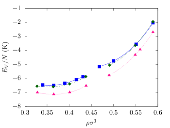
Figure 1: Ground-state energies as a function of the density for the liquid and solid phases of a system formed from ⁴He atoms. Blue squares represent our results and the solid blue line is a fit to the computed values. The green diamonds and the dashed green line are the reported results in Ref. MacFarland et al., 1994. In both phases pink triangles stand for fits to values obtained by neutron scattering experiments. The dotted pink line represent the fitting of these data. In the liquid phase the fit is the one by Aziz and PathriaAziz and Pathria (1973). For solid helium we have fitted the data from Woods et al.Woods and Sears (1977).

Table 3: Adjusted coefficients $A$, $B$ and $C$ in units of K and $\rho_{0}$ in units of $\sigma^{-3}$, of Eq. (18), the polynomial fit to the variational energies.

	$A$	$B$	$C$	$\rho_{0}$
Liquid	-6.51	17.70	-15.57	0.357
Solid	-5.42	-0.01	19.45	0.378

In the solid phase we can see that as the density increases, our energy becomes marginally lower than the results of MacFarland et al. MacFarland et al. (1994). To some extent a similar behavior can also be seen in the liquid state where as the density increases we see our variational energies approaching those of Ref. MacFarland et al., 1994. Since in our trial function the sampling of exchange between atoms is more efficiently done, these results suggest that the importance of exchange increases with the density.

IV.3 Melting-Freezing Transition

The melting and freezing densities are easily determined through the EOS of the liquid and solid phases using the double tangent Maxwell construction, Eq. (19). The value we have estimated for the freezing density is $\rho_{f}=0.457\ \sigma^{-3}$. It can be compared with the experimental value of 0.431 $\sigma^{-3}$. For the melting transition our calculation gave $\rho_{m}=0.495\ \sigma^{-3}$ and experiment 0.468 $\sigma^{-3}$. Although our melting transition density is about of the same quality obtained with a shadow function with optimized two-body correlations between atoms Moroni et al. (1998), our freezing density it not so good.

IV.4 Radial distribution functions

The radial distribution functions $g(r)$ computed at four densities in the liquid phase is shown in Fig. 2. The figure on the left is the radial distribution function of the atoms of The shadow particles, that model the center of mass of polymers of the Feynman path-integral in imaginary time reflect somewhat the more classical behavior of this particles. This is also the behavior we see for the shadows in the crystal case displayed in Fig. 3. It is visible the formation of a small shoulder before the second peak typically seen in the crystallization process of classical fluids. The radial distribution of the atoms in the solid phase displayed at the same figure show more structure than the liquid phase. However it is much less pronounced than in classical solids.

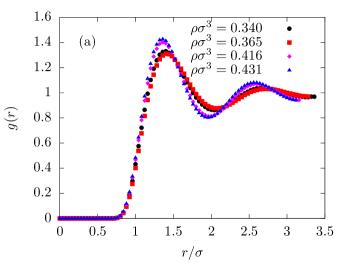
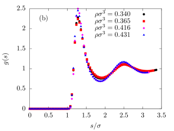
Figure 2: Radial distribution of atoms $g(r)$ (a) and auxiliary variables $g(s)$ (b) at four densities in the liquid phase of the ⁴He system. As expected the system turns out to have more structure as the density increases. Shadow particles have peaks much more intense.

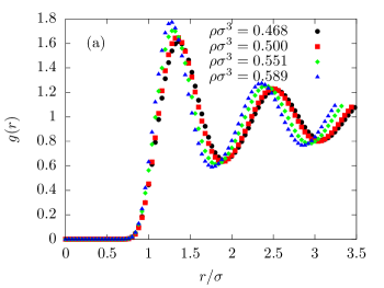
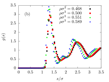
Figure 3: Radial distribution of atoms $g(r)$ (a) and auxiliary variables $g(s)$ (b) at four densities of the ⁴He in the solid phase.

It is also interesting to compare our results for the radial function of atoms to those obtained by the GFMC methodKalos et al. (1981) that gives essentially the exact results. This is made in Fig. 4. It is worth to mention that the inter-atomic potential we use Aziz et al. (1995) is a more recent one. It does not include in an effective way three-body contributions like the one Aziz et al. (1979) employed in the GFMC calculation. The agreement of the results in the liquid phase are very good despite the difference of the potentials used in the two calculations. At the solid phase at the density $\rho=0.589\sigma^{-3}$ there is a remarkable agreement as we can see in Fig. 4(b). It is at this density that our trial function outperform shadow functions without an explicit symmetric kernel.

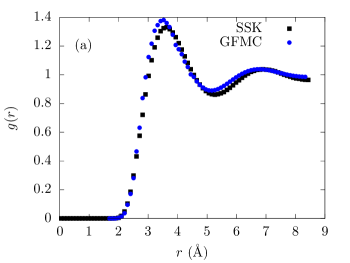
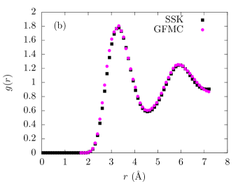
Figure 4: Comparison of $g(r)$ determined with the $\Psi_{SSK}$ trial function (black squares) with GFMC results (blue and pink circles) from Kalos et al. Kalos et al. (1981) for ⁴He systems. For the liquid phase (a) the calculations are at the experimental equilibrium density $\rho=0.365\sigma^{-3}$ and for the crystal phase (b) at $\rho=0.589\sigma^{-3}$.

IV.5 Condensate fraction

The single particle momentum distribution $n(k)$ characterizes the extent a system formed from ⁴He have a behavior that deviates from classical physics. The strong quantum effects present in this system does not allow a description in terms of the Maxwell-Boltzmann distribution, typical of classical systems. A related quantity, the off-diagonal matrix element of the one-body density matrix, $\rho_{1}(r)$ can be calculated straightforward through Eq. (21). At the equilibrium experimental density $\rho=0.365\sigma^{-3}$, our results are shown in Fig. 5 from where we have extracted $n_{0}=(3.57\pm 0.07)\%$ for the condensate fraction. We have computed this quantity at other densities as well, the results together with experimental measures Glyde et al. (2011a) are displayed in Fig. 6.

Figure 5: The one-body density matrix estimated using Eq. (21) at the experimental equilibrium density $\rho=0.365\sigma^{-3}$.

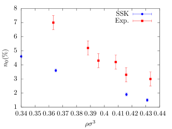
Figure 6: The condensate fraction estimated trough the sampling of ${\cal P}(R,S,S^{\prime})$ at four densities at the liquid phase compared with experimental results extracted from Ref. Glyde et al., 2011b.

At the equilibrium density the theoretical and experimental values of the condensate fraction differ by a factor of about 2. This fact lead us to consider the question of how efficient the sampling of Eq. (10) can be for the condensate fraction estimation. For this reason we have also considered sampling the probability distribution function of Eq. (24) to compute $\rho_{1}(r)$. Its normalization factor can be obtained from Fig. 5 by considering small values of $r$. The normalized result of $\rho_{1}(r)$ determined in this way is presented in Fig. 7. From this calculation the associated condensate fraction is equal to $n_{0}=(8.17\pm 0.03)\%$. A value in much better agreement with the experimental dataGlyde et al. (2011b), $(7.25\pm 0.75)\%$.

Although we are in front the apparent puzzle of having two different values for the estimation of a given property (the condensate fraction), it is possible to explain these results. The shadow particles create about themselves through the Jastrow factor $\psi_{s}$ a much larger exclusion volume than the one of the atoms. This situation produces a jam in their moves. For feasible computational times the shadow particles are not able to effectively explore the phase space available to them. Certainly, if we could wait for the shadow moves through their jam, both ways of computing the single particle momentum distribution would agree. The result of Fig. 5 are due only to the symmetrization we have introduced in our trial function but does not take into account, or maybe takes only partially, the possibility of the diffusion of the shadow particles in their configuration space.

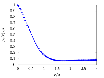
Figure 7: The normalized one body density function obtained by sampling Eq. (24). The associated condensate fraction is $(8.17\pm 0.03)$ at the experimental equilibrium density.

For completeness and to be careful with our results we have also investigated how finite size effects of the simulation box might affect the condensate fraction calculations when we sample the probability density function of Eq. (24). We carried out simulations for systems of 32, 64 and 108 bodies at the experimental equilibrium density $\rho=0.365\sigma^{-3}$. The results are shown in Table 4. From our results it is possible to say that with 64 bodies finite size effects most probably are negligible. Nevertheless all the reported results were obtained considering $N=108$ bodies.

Table 4: The condensate fraction $n_{0}$ estimated for systems of 32, 64 and 108 bodies at the experimental equilibrium density ($\rho\sigma^{3}=0.365$).

$N$	32	64	108
$n_{0}$ ($\%$)	$9.2\pm 0.4$	$8.3\pm 0.1$	$8.17\pm 0.03$

V Final comments

The shadow wave function is a powerful tool to investigate quantum liquids and solids formed from helium atoms. Since its inception Vitiello et al. (1988), steady progress has been made. First an attractive pseudo-potential and optimized two-body correlations were introduced MacFarland et al. (1994). Later it was extended to treat the fermionic system made from ³He atoms Pederiva et al. (1996). More recently Dandrea et al. (2009) a much more sophisticated approach to the last problem was introduced where the antisymmetric character of the wave function was introduced trough the auxiliary variables themselves. In this work we have modifyied the atom-shadow coupling by introducing an explicitly symmetric kernel and analyzed its consequences. In a formal way this approach does change basic properties of this class of trial functions like translational and its symmetrical character. However it was possible to demonstrate that exchange correlations becomes more important as the density increases. We have also shown the need of considering in an explicit way the jam created by the shadow particles in the liquid phase for computing the condensate. As we increase the density in the solid phase we are able to improve the variational energy with respect to a kernel not symmetric. The shadow function has implicit correlations up to the number of particles considered in the system. We believe that attempts to optimize these correlations are important because they might help to uncover yet unknown properties of the systems formed from helium atoms.