Exotic looped trajectories in double-slit experiments with matter waves

Abstract

We study the observation of exotic looped trajectories in double-slit experiments with matter waves. We consider the relative intensity at $x=0$ as a function of the time-of-flight from the double-slit to the screen inside the interferometer. This allows us to define a fringe visibility associated to the contribution to the interference pattern given by exotic lopped trajectories. We demonstrate that the Sorkin parameter is given in terms of this visibility and of the axial phases which include the Gouy phase. We verify how this parameter can be obtained by measuring the relative intensity at the screen. We show that the effect of exotic looped trajectories can be significantly increased by simply adjusting the parameters of the double-slit apparatus. Applying our results to the case of neutron interferometry, we obtain a maximum Sorkin parameter of the order of $|\kappa_{max}|\approx 0.2$, which is the value of the fringe visibility.

I Introduction

The first theoretical study of the effects of exotic trajectories (also called non-classical paths) in two-slit interferometry dates back to 1986 in the work by H. Yabuki Yabuki . The Feynman path integral approach FeynmanHibbs was used there to include all possible paths of the interfering object from the source to the screen passing through the double-slit. Some of such paths are the looped trajectories along the slits, i.e., exotic looped trajectories. However, the probability associated with such trajectories is much smaller than the probability associated with the non-exotic trajectories (also called classical paths) which are considered in the usual setup for the double-slit experiment. Experimental access to such tiny deviations was later discussed by Sorkin Sorkin , in a work where higher-order contributions when three or more paths interfere are incorporated to the usual prescription for two-slit interference. The first observation of these effects was obtained by Sinha et al. in a triple-slit interference experiment with photons Sinha1 . In that experiment such effects were interpreted as third-order quantum interference, which means a violation of Born’s rule. But De Raedt et al. showed that such deviations can exist without any such violation Raedt . Further, Sinha et al. reported that the deviation observed in that experiment could be a consequence of exotic looped trajectories along the slits and not a violation of Born’s rule Sinha2 ; Sinha3 . However, the third-order quantum interference has been recently shown with a single spin in solids, confirming the violation Jin . Also, it was demonstrated that a double-slit experiment equipped with which-way detectors can also violate Born’s rule Quach . Therefore, it is possible that effects from both types of deviations are present – those coming from exotic looped trajectories, as well as from a Born’s rule violation.

In Ref. Sinha2 the contribution of exotic trajectories to triple-slit matter wave diffraction was evaluated using the Feynman path integral approach with a free propagator given by $K(\vec{r},\vec{r}^{\prime})=\frac{k}{2\pi i}\frac{1}{|\vec{r}-\vec{r}^{\prime}|}\;e^{ik|\vec{r}-\vec{r}^{\prime}|}$ (which satisfies the Helmholtz equation away from $\vec{r}=\vec{r}^{\prime}$ and the Fresnel-Huygens principle). In the Fraunhofer regime this leads to integrals which were evaluated numerically using the stationary phase approximation. As a result, the authors obtained a Sorkin parameter of order $\kappa\approx 10^{-8}$ for electron waves. However, new experiments with three slits proposed in Sinha3 using matter waves or low frequency photons were analytically described, giving an upper bound on the Sorkin parameter by $|\kappa_{\mathrm{max}}|\approx 0.003\lambda^{3/2}/(d^{1/2}w)$, in which $\lambda$ is the wavelength, $d$ is the center-to-center distance between the slits, and $w$ is the slit width. They confirmed that the Sorkin parameter $\kappa$ is very sensitive to the experimental setup.

Recently, an analytical treatment was given for exotic looped trajectories in the triple-slit experiment Paz3 . The wave functions with all the phases corresponding to both exotic and non-exotic trajectories were analytically obtained using non-relativistic propagators for a free particle. This procedure enabled the authors to incorporate the effect of the Gouy phase into the Sorkin parameter $\kappa$. The effect was indicated on the interference pattern as well as in $\kappa$ for the case of matter waves. Moreover, this framework allowed the derivation of an expression for $\kappa$ which is of order $10^{-8}$ for electron waves. Using the three-slit experimental setup it was thus possible to compare the order of magnitude of $\kappa$ to the value obtained in Sinha2 for the same input data, with agreement for electron waves.

The existence of exotic looped trajectories was recently observed for photons by Boyd et al. in Ref. BoydNat . They used the three-slit setup and showed that looped trajectories of photons are physically due to the near-field component of the wavefunction, which leads to an interaction among the three slits. Thus, they conclude that is possible to increase the probability of occurrence of these trajectories by controlling the strength and spatial distribution of the electromagnetic near-fields around the slits.

Double-slit is a simple experimental setup often used to demonstrate fundamental aspects of quantum theory Feynman . Double-slit experiments enabled us to observe wave-particle duality with electrons Jonsson , neutrons Zeilinger1 , and atoms Carnal . Also, probability distributions for single- and double-slit arrangements were observed in a controlled electron double-slit diffraction Bach . For the triple-slit experiment studied previously, we can have deviations in the interference pattern produced by both the exotic trajectories and third-order interference. On the other hand, for the usual double-slit experiment, only effects due to exotic trajectories can be present. Until the present time such effects have not been investigated in the double-slit setup. In the present paper, we present the first study of exotic looped trajectories in the double-slit experiment. We analyze quantitatively the observation of exotic trajectory effects in the interference pattern for massive particles. We follow the treatment used in Ref. Paz3 and obtain analytically all wavefunctions and phases. The analytical expressions for the relative intensity and Sorkin parameter enables us to make some useful approximations. As we discuss here, the advantage of the double-slit compared to the triple-slit setup is that it allows one to reduce the amount of terms in the description of interference, leading to expressions more simple to interpret. Thus, we are able for example to relate the Sorkin parameter to the visibility produced by exotic trajectories, and to show that exotic trajectory effects can be accessed by measuring the relative intensity. These simpler expressions also show that it is possible to increase such exotic effect by carefully adjusting some of the double-slit parameters.

This contribution is organized as follows: in section II we obtain analytical expressions for the wavefunctions for both exotic and non-exotic trajectories, calculate the relative intensity, and estimate the deviations produced by exotic trajectories through the Sorkin parameter $\kappa$. In section III we consider the position $x=0$ in the detection screen and analyze both the relative intensity and Sorkin parameter as functions of the time-of-flight from the double-slit to the screen. We also describe how the Sorkin parameter can be obtained by measuring the relative intensity. In section IV, we show how it is possible to significantly increase the Sorkin parameter by simply adjusting some parameters of the double-slit apparatus. We observe that the maximum of the Sorkin parameter can be obtained by measuring the fringe visibility. A few concluding remarks are finally presented in section V.

II Double-slit experiment with exotic looped trajectories

In this section we will describe the double-slit experiment with exotic looped trajectories, and obtain analytically the wave functions corresponding to both the non-exotic (paths $1$ and $2$) and the exotic looped trajectories (paths $12$ and $21$), as illustrated in the experimental setup of figure 1. We will also calculate the relative intensity and the Sorkin parameter $\kappa$ in the screen of detection as a function of the position $x$.

As in the previous paper Paz3 , we assume a one dimensional model in which quantum effects are manifested only in the $x$-direction. A coherent Gaussian wavepacket of initial transverse width $\sigma_{0}$ is produced in the source $S$ and propagates up to time $t$ before arriving at a double-slit with Gaussian apertures, from which Gaussian wavepackets propagate. After crossing the grid, the wavepackets propagate during a time interval given by $\tau$ before arriving at detector $D$. This gives rise to a interference pattern as a function of the transverse coordinate $x$. Quantum effects are realized only in the $x$-direction, as we consider that the energy associated with the momentum of the particles in the $z$-direction is very high, in such a way that the momentum component $p_{z}$ is sharply defined, i.e., $\Delta p_{z}\ll p_{z}$. Then we can consider that we have a classical motion in this direction, at velocity $v_{z}$. Because the propagation is free, the $x$, $y$ and $z$ dimensions decouple for a given longitudinal location, and thus we may write $z=v_{z}t$. As $v_{z}$ is assumed to be a well defined velocity we can neglect statistical fluctuations in the time-of-flight, i.e., $\Delta t\ll t$. Such approximation leaves the Schrödinger equation analogous to the optical paraxial Helmholtz equation Viale ; Berman . The summation over all possible trajectories allows for exotic paths such as the paths $12$ and $21$ depicted in figure 1.

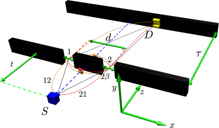
Figure 1: Sketch of the double-slit experiment with exotic looped trajectories. A Gaussian wavepacket of transverse width $\sigma_{0}$ is produced at the source $S$, propagates a time $t$ before reaching the double-slit, and a time $\tau$ from the double-slit to the detector $D$. The slit apertures are taken to be Gaussian, of width $\beta$ and separated by a distance $d$. The paths $1$, $2$ are non-exotic paths and the paths $12$ (orange line or clockwise loop) and $21$ (red line or counterclockwise loop) are looped trajectories, or exotic paths.

The wave function for the non-exotic trajectories $1$ and $2$ (black lines) are given by

$$\psi_{1,2}(x,t,\tau) = \int_{x_{j},x_{0}}K_{\tau}(x,t+\tau;x_{j},t)F(x_{j}\pm d/2)$$ (1)

$$\times K_{t}(x_{j},t;x_{0},0)\psi_{0}(x_{0}),$$

where

$$K(x_{j},t_{j};x_{0},t_{0})=\sqrt{\frac{m}{2\pi i\hbar(t_{j}-t_{0})}}\exp\left[\frac{im(x_{j}-x_{0})^{2}}{2\hbar(t_{j}-t_{0})}\right],$$

$$F(x_{j})=\exp\left[-\frac{(x_{j})^{2}}{2\beta^{2}}\right],$$

and

$$\psi_{0}(x_{0})=\frac{1}{\sqrt{\sigma_{0}\sqrt{\pi}}}\exp\left(-\frac{x_{0}^{2}}{2\sigma_{0}^{2}}\right).$$

In the above, the kernels $K_{t}(x_{j},t;x_{0},0)$ and $K_{\tau}(x,t+\tau;x_{j},t)$ are the free propagators for the particle, the functions $F(x_{j})$ describe the slit transmission functions which are taken to be Gaussian of width $\beta$ separated by a distance $d$; $\sigma_{0}$ is the effective width of the wavepacket emitted from the source $S$, $m$ is the mass of the particle, $t$ ($\tau$) is the time-of-flight from the source (double-slit) to the double-slit (screen).

The wavefunction associated with the exotic trajectory $12$ (orange line or clockwise loop) is given by

$$\psi_{\mathrm{et}12}(x,t,\tau)=\int_{x_{0},x_{1},x_{2},x_{3}}K_{\tau}(x,\tau+\tilde{t};x_{3},\tilde{t})$$

$$\,\times F(x_{3}+d/2)F(x_{2}-d/2)K(1\rightarrow 2;2\rightarrow 1)$$

$$\times\,F(x_{1}+d/2)K_{t}(x_{1},t+\eta;x_{0},0)\psi_{0}(x_{0}),$$ (2)

where $\tilde{t}=t+2\epsilon$, and where

$$K(1\rightarrow 2;2\rightarrow 1)=\sqrt{\frac{m}{4\pi i\hbar(\epsilon+\eta)}}\times$$

$$\exp\left[\frac{im[(x_{2}-x_{1})^{2}+(x_{3}-x_{2})^{2}]}{4\hbar(\epsilon+\eta)}\right],$$ (3)

denotes the free propagator which propagates from slit $1$ to slit $2$ and from slit $2$ to slit $1$. The parameter $\eta\rightarrow 0$ is an auxiliary inter slit time parameter, and $\epsilon$ denotes the time spent from one slit to the next and is determined by the momentum uncertainty in the $x$-direction, i.e., $\epsilon=\frac{d}{\Delta v_{x}}$ ($\Delta v_{x}=\Delta p_{x}/m$), with $\Delta p_{x}=\sqrt{\langle\hat{p}^{2}_{x}\rangle-\langle\hat{p}_{x}\rangle^{2}}$, $\hat{p}_{x}$ being the momentum operator in the $x$-direction. The time $\epsilon$ is a statistical fluctuation on the time for motion in the $x$-direction, which has to attain a minimum value $d/\Delta v_{x}$ in order to guarantee the existence of a exotic trajectory Paz3 .

After some lengthy algebraic manipulations, we obtain:

$$\psi_{1}(x,t,\tau)=A\exp\left(-C_{1}x^{2}-C_{2}x+C_{3}\right)$$ (4)

$$\times\exp\left(i\alpha x^{2}-i\gamma x+i\theta+i\mu\right),$$

$$\psi_{2}(x,t,\tau)=A\exp\left(-C_{1}x^{2}+C_{2}x+C_{3}\right)$$ (5)

$$\times\exp\left(i\alpha x^{2}+i\gamma x+i\theta+i\mu\right),$$

and

$$\psi_{\mathrm{et}12}(x,t,\tau)=A_{\mathrm{et}}\exp\left(-C_{1\mathrm{et}}x^{2}-C_{2\mathrm{et}}x+C_{3\mathrm{et}}\right)$$ (6)

$$\times\exp\left(i\alpha_{\mathrm{et}}x^{2}-i\gamma_{\mathrm{et}}x+i\theta_{\mathrm{et}}+i\mu_{\mathrm{et}}\right).$$

The phases $\mu$ and $\mu_{\mathrm{et}}$ are Gouy phases Gouy for non-exotic and exotic trajectories, respectively. We use the subscript (et) for quantities related with exotic trajectories, and no subscript for quantities related with non-exotic trajectories. This convention will be used in what follows.

The wave function for the exotic trajectory $21$ (red line or counterclockwise loop) is obtained by substituting $d$ by $-d$ in Eq. (6), which is given by

$$\psi_{\mathrm{et}21}(x,t,\tau)=A_{\mathrm{et}}\exp\left(-C_{1\mathrm{et}}x^{2}+C_{2\mathrm{et}}x+C_{3\mathrm{et}}\right)$$

$$\times\exp\left(i\alpha_{\mathrm{et}}x^{2}+i\gamma_{\mathrm{et}}x+i\theta_{\mathrm{et}}+i\mu_{\mathrm{et}}\right).$$ (7)

All the coefficients present in equations (4)-(II) are written out in Appendices 1 and 2 for the sake of clarity. The indices $R$ and $I$ stand for the real and imaginary part of the complex numbers that appear in the solutions. As discussed in Paz2 , $\mu_{\mathrm{et}}(t,\tau)$ and $\theta_{\mathrm{et}}(t,\tau)$ are phases that do not depend of the transverse position $x$, i.e., they are axial phases. Different from the Gouy phase, $\theta_{\mathrm{et}}(t,\tau)$ is a phase that appears as we displace the slit from a given distance away from the origin, which is dependent on the parameter $d$.

The total intensity at a give position $x$ in the detection screen including the contribution of both exotic and non-exotic trajectories is given by Born’s rule Born

$$I_{T}=|\psi_{1}+\psi_{2}+\psi_{\mathrm{et}12}+\psi_{\mathrm{et}21}|^{2},$$ (8)

which allows us to obtain the following result:

$$I_{T}(x,t,\tau)=|\psi_{1}|^{2}+|\psi_{2}|^{2}+|\psi_{\mathrm{et}12}|^{2}+|\psi_{\mathrm{et}21}|^{2}$$

$$+2|\psi_{1}||\psi_{2}|\cos(\phi_{1,2})$$

$$+2|\psi_{1}||\psi_{\mathrm{et}12}|\cos(\phi_{1,\mathrm{et}12})$$

$$+2|\psi_{1}||\psi_{\mathrm{et}21}|\cos(\phi_{1,\mathrm{et}21})$$

$$+2|\psi_{2}||\psi_{\mathrm{et}12}|\cos(\phi_{2,\mathrm{et}12})$$

$$+2|\psi_{2}||\psi_{\mathrm{et}21}|\cos(\phi_{2,\mathrm{et}21})$$

$$+2|\psi_{\mathrm{et}12}||\psi_{\mathrm{et}21}|\cos(\phi_{\mathrm{et}12,21}),$$ (9)

with the phase differences being given by

$$\phi_{1,2}=2\gamma x,$$ (10)

$$\phi_{1,\mathrm{et}12}=(\alpha-\alpha_{\mathrm{et}})x^{2}-(\gamma-\gamma_{\mathrm{et}})x+(\theta-\theta_{\mathrm{et}})+(\mu-\mu_{\mathrm{et}}),$$ (11)

$$\phi_{1,\mathrm{et}21}=(\alpha-\alpha_{\mathrm{et}})x^{2}-(\gamma+\gamma_{\mathrm{et}})x+(\theta-\theta_{\mathrm{et}})+(\mu-\mu_{\mathrm{et}}),$$ (12)

$$\phi_{2,\mathrm{et}12}=(\alpha-\alpha_{\mathrm{et}})x^{2}+(\gamma+\gamma_{\mathrm{et}})x+(\theta-\theta_{\mathrm{et}})+(\mu-\mu_{\mathrm{et}}),$$ (13)

$$\phi_{2,\mathrm{et}21}=(\alpha-\alpha_{\mathrm{et}})x^{2}+(\gamma-\gamma_{\mathrm{et}})x+(\theta-\theta_{\mathrm{et}})+(\mu-\mu_{\mathrm{et}}),$$ (14)

and

$$\phi_{\mathrm{et}12,21}=2\gamma_{\mathrm{et}}x\,.$$ (15)

From the total intensity Eq. (9) we calculate the relative intensity $I_{r}=I_{T}(x,t,\tau)/F(x,t,\tau)$ and obtain the following result:

$$I_{r}(x,t,\tau)=1+(2/F)|\psi_{1}||\psi_{2}|\cos(\phi_{1,2})$$

$$+(2/F)|\psi_{1}||\psi_{\mathrm{et}12}|\cos(\phi_{1,\mathrm{et}12})$$

$$+(2/F)|\psi_{1}||\psi_{\mathrm{et}21}|\cos(\phi_{1,\mathrm{et}21})$$

$$+(2/F)|\psi_{2}||\psi_{\mathrm{et}12}|\cos(\phi_{2,\mathrm{et}12})$$

$$+(2/F)|\psi_{2}||\psi_{\mathrm{et}21}|\cos(\phi_{2,\mathrm{et}21})$$

$$+(2/F)|\psi_{\mathrm{et}12}||\psi_{\mathrm{et}21}|\cos(\phi_{\mathrm{et}12,21}),$$ (16)

where

$$F(x,t,\tau) = |\psi_{1}(x,t,\tau)|^{2}+|\psi_{2}(x,t,\tau)|^{2}$$ (17)

$$+ |\psi_{\mathrm{et}12}(x,t,\tau)|^{2}+|\psi_{\mathrm{et}21}(x,t,\tau)|^{2}\,.$$

Now, in order to estimate the effect of exotic looped trajectories we use the definition of the Sorkin parameter of Ref. Paz3 , obtaining

$$\kappa(x,t,\tau)=\frac{I_{T}(x,t,\tau)-I(x,t,\tau)}{I_{max}}$$

$$=(1/I_{max})(|\psi_{\mathrm{et}12}|^{2}+|\psi_{\mathrm{et}21}|^{2})$$

$$+(2/I_{max})|\psi_{1}||\psi_{\mathrm{et}12}|\cos(\phi_{1,\mathrm{et}12})$$

$$+(2/I_{max})|\psi_{1}||\psi_{\mathrm{et}21}|\cos(\phi_{1,\mathrm{et}21})$$

$$+(2/I_{max})|\psi_{2}||\psi_{\mathrm{et}12}|\cos(\phi_{2,\mathrm{et}12})$$

$$+(2/I_{max})|\psi_{2}||\psi_{\mathrm{et}21}|\cos(\phi_{2,\mathrm{et}21})$$

$$+(2/I_{max})|\psi_{\mathrm{et}12}||\psi_{\mathrm{et}21}|\cos(\phi_{\mathrm{et}12,21}),$$ (18)

where $I$ is the intensity when we consider only non-exotic trajectories and $I_{max}$ is the intensity in the position $x=0$, the central maximum. As we can observe from Eq.(16), some terms in the relative intensity are analogous to the terms of the Sorkin parameter for $x=0$, but they differ a lot for other values of $x$. This happens because the factor $F$ is $x$ dependent and $I_{max}$ is $x$ independent. Therefore, it is not possible to obtain $\kappa$ by measuring the relative intensity as a function of $x$. This can be different if we consider the position $x=0$ and change the value of the time variable $\tau$.

The results obtained above for the relative intensity and Sorkin parameter depend in both cases on the parameter $\epsilon$. Therefore, in order to plot these quantities, we need to know $\epsilon$. From the wave function $\psi_{1}(x,t,\tau)$ (one can also use the wave function $\psi_{2}(x,t,\tau)$), we calculate the uncertainty in momentum and obtain for the $\epsilon$ the following result:

$$\epsilon(\sigma_{0},\beta,t,d,m)=\frac{m\beta d}{\hbar}\sqrt{\frac{1+(\beta/\sigma_{0})^{2}+(t/\tau_{0})^{2}}{[1+(\beta/\sigma_{0})^{2}]^{2}+(t/\tau_{0})^{2}}}.$$ (19)

Notice that this quantity depends on the mass of the particle and on the parameters of the double-slit. Fortunately, this parameter is independent of $\tau$ as expected, since the propagation from the double-slit to the screen is free. This independence will be further useful to study the exotic trajectory contribution as a function of $\tau$.

We consider the neutron parameters previously used in interference experiments, such as $m=1.67\times 10^{-27}\;\mathrm{kg}$, $\sigma_{0}=7.0\;\mathrm{\mu m}$, $d=125\;\mathrm{\mu m}$, $\beta=7.0\;\mathrm{\mu m}$, $t=18\tau_{0}$ and $\tau=18\tau_{0}$. For these parameters we obtain $\epsilon=19.5\;\mathrm{ms}$. In figure 2(a) we show the relative intensity and in figure 2(b) the Sorkin parameter as a function of $x$.

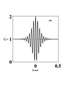
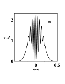
Figure 2: (a) Relative intensity, and (b) Sorkin parameter as a function of $x$. The magnitude of the Sorkin parameter is $10^{-6}$.

We can see that the relative intensity is maximum at $x=0$, with maximum $I_{r}=2$, and oscillate around the classical result (no interference) $I_{r}=1$. For large value of $x$ we do not have interference and $I_{r}(x>0.5\;\mathrm{mm})=1$. The oscillation of the relative intensity for $|x|<0.5\;\mathrm{mm}$ contains contributions of exotic and non-exotic trajectories. Figure 2(b) shows that the contribution of exotic looped trajectories to the relative intensity is of the order of $\kappa\approx 10^{-6}$, and the main contribution to the oscillation is produced by the non-exotic trajectories. We observe that the chosen set of parameter values led to a Sorkin parameter two orders of magnitude bigger than the values previously obtained in the literature for electron waves in Sinha2 ; Paz3 , showing that neutron interferometry offers a better candidate for the study of exotic looped trajectory effects than interference experiments with electrons.

III Fringe visibility and Sorkin parameter

In this section we will fix the position at $x=0$, i.e., along the symmetry axis of the double-slit, and obtain simple expressions to the relative intensity and Sorkin parameter as a function of $\tau$ (or distance $z_{\tau}$ from the double-slit to the screen, since we are considering that $z_{\tau}=v_{z}\tau$). This allows us to define the visibility associated to the exotic trajectory contribution, and show that the Sorkin parameter can be written in terms of the visibility. As we will see, measuring the Sorkin parameter under some conditions means measuring the visibility of the exotic trajectory contribution.

At the position $x=0$, we have $\phi_{1,\mathrm{et}12}=\phi_{2,\mathrm{et}12}=\phi_{1,\mathrm{et}21}=\phi_{2,\mathrm{et}21}=(\theta_{\mathrm{et}}+\mu_{\mathrm{et}})-(\theta+\mu)$, $\phi_{1,2}=\phi_{\mathrm{et}12,21}=0$, $|\psi_{1}|=|\psi_{2}|$ and $|\psi_{\mathrm{et}12}|=|\psi_{\mathrm{et}21}|$. The parameters $\sigma_{0}$, $\beta$, $d$, $t$, $\tau$ and $\epsilon$ can be set such that we have $|\psi_{1}(0,t,\tau)|\gg|\psi_{\mathrm{et}12}(0,t,\tau)|$, giving

$$F(0,t,\tau)\approx 2|\psi_{1}(0,t,\tau)|^{2}.$$ (20)

Under these conditions, the relative intensity Eq. (16) can be written as

$$I_{r}(0,t,\tau)\approx 2\{1+\mathcal{V}_{\mathrm{et}}(0,t,\tau)\cos[\theta_{\mathrm{et}}+\mu_{\mathrm{et}}-(\theta+\mu)]\},$$ (21)

where

$$\mathcal{V}_{\mathrm{et}}(0,t,\tau)=\frac{2|\psi_{\mathrm{et}12}(0,t,\tau)|}{|\psi_{1}(0,t,\tau)|}.$$ (22)

The relative intensity Eq. (21) has an expression similar to Eq. (1.3) in Bramon, Ref. Bramon , enabling us to identify the function $\mathcal{V}_{\mathrm{et}}$ as being the visibility. More interestingly here, this visibility is constructed with exotic wave functions. The second term of Eq. (21) is the interference produced by the exotic trajectory contribution. If we neglect this contribution we would have $I_{r}=2$, which is indeed the relative intensity when we consider only non-exotic trajectories. Therefore, when we consider $x=0$ the measurement of the relative intensity as a function of $\tau$ enables us to obtain the exotic trajectory contribution to the interference. It is important to observe that the interference as a function of $\tau$ is a result of the both the exotic and non-exotic phases, in such a way that the oscillation of the relative intensity for $x=0$ indicates the existence of exotic trajectories.

It is easy to show that the second term of Eq. (21) is the Sorkin parameter used previously to estimate the effect of the exotic contribution to the interference. By putting the intensity at the central maximum $I_{max}=I_{T}(0,t,\tau)\approx 4|\psi_{1}|^{2}$ in the definition of the Sorkin parameter, Eq. (18), for $x=0$ we obtain

$$\kappa = \mathcal{V}_{\mathrm{et}}(0,t,\tau)\cos[\theta_{\mathrm{et}}+\mu_{\mathrm{et}}-(\theta+\mu)],$$ (23)

which depends on the visibility of exotic trajectory contribution as well as on the axial phases. Notice that this result is true only for $x=0$. For $x=0$, measurement of the relative intensity gives the Sorkin parameter.

In order to obtain an estimate of the exotic trajectory contribution, we consider the neutron parameters as before, except that here we change the parameter $\tau$ and maintain the position at $x=0$. As shown in the previous section, the parameter $\epsilon$ remains constant when $\tau$ changes. This property is important for the construction of our results. In figure 3(a) we show the relative intensity and in figure 3(b) the Sorkin parameter as a function of $\tau$. We can observe that $(I_{r}/2)-1=\kappa\approx 10^{-6}$, which have the same order of magnitude when plotted as a function of $x$. Thus, although we can obtain the Sorkin parameter by measuring the relative intensity, a very good measurement precision is required.

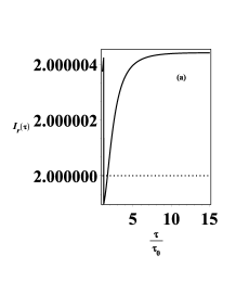
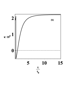
Figure 3: (a) Relative intensity and (b) Sorkin parameter as a function of $\tau$. The magnitude of the Sorkin parameter is $10^{-6}$ the same order of its magnitude as a function of $x$.

The results above show that although the measurement of the relative intensity can be useful to observe the contribution of exotic trajectories in the interference pattern, its small value persist. Therefore, observation of effects from exotic trajectories may require the use of some mechanism to amplify the small value of the Sorkin parameter. Such a mechanism will be discussed in the next section.

IV Increasing the Sorkin parameter

It was observed in Sinha3 that the Sorkin parameter is very sensitive to the parameters of the experimental setup. They obtain an expression for the maximum value of the Sorkin parameter that include the wavelength $\lambda$, the separation between the slits $d$ and the slit width $\beta$. Therefore, in order to increase the Sorkin parameter we change the neutron parameters $\beta$ and $d$ and choose $\beta=12\;\mathrm{\mu m}$ and $d=475\;\mathrm{\mu m}$, while maintaining all the other parameters constant. For these new parameters, we obtain $\epsilon=132\;\mathrm{ms}$. Moreover, for this set of parameter values the validity of our approximations is guaranteed. In figure 4(a) we show the relative intensity and in figure 4(b) we show the Sorkin parameter as a function of $\tau$. Since we are considering classical motion in the $z$-direction, we have $z_{\tau}=v_{z}\tau$. Thus, fixing the distance $z_{\tau}$ and changing $\tau$ is equivalent to changing the velocity $v_{z}$ or the wavelength $\lambda=h/mv$ ($h$ is the Planck constant), since $v=\sqrt{v_{x}^{2}+v_{z}^{2}}\approx v_{z}$ for paraxial matter waves Berman . Changing the wavelength in order to obtain a maximum value to the Sorkin parameter also agrees with the result obtained in Sinha3 . We use a dotted line to represent the result when we have only non-exotic trajectories contribution, i.e., $\kappa=0$ and $I_{r}=2$. We observe that the relative intensity differs from the value $2$ by the maximum value $0.4$, which corresponds to a maximum value of the Sorkin parameter $|\kappa_{max}|=|(I_{r}/2)-1|\approx 0.2$. Therefore, it is possible to increase the contribution from exotic trajectories to the experimental reality by only changing some parameters of the double-slit setup, as proposed in Sinha3 .

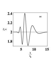
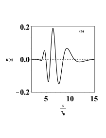
Figure 4: (a) Relative intensity and (b) Sorkin parameter as a function of $\tau$. We observe an increase in the Sorkin parameter, with a maximum value of the order of $|\kappa_{max}|\approx 0.2$. The dotted line corresponds to the result when we have only the non-exotic trajectories contribution, i.e., $\kappa=0$ and $I_{r}=2$.

We can observe from Eq. (23) that the value of the Sorkin parameter depends on the axial phase, which caries exotic and non-exotic trajectories contribution. The maximum value of this parameter occurs for $[\theta_{\mathrm{et}}+\mu_{\mathrm{et}}-(\theta+\mu)]=2n\pi$ ($n=0,1,2...$), which is exactly the fringe visibility. On the order hand, for $[\theta_{\mathrm{et}}+\mu_{\mathrm{et}}-(\theta+\mu)]=(2n+1)(\pi/2)$ ($n=0,1,2...$) we have $\kappa=0$, and no contribution of exotic trajectories will be observed, as represented by the dotted line of figure 4(b). Therefore we can observe or not the effect of exotic trajectories depending on the value of the axial phases. We can also observe in figure 4 that for $\tau\gg\tau_{0}$ we have only non-exotic contributions, which is a consequence of the fact that $\mathcal{V}_{\mathrm{et}}(0,t,\tau\gg\tau_{0})\rightarrow 0$. We would like to point out that special attention should be given to points where the Sorkin parameter has a maximum, i.e., $|\kappa_{max}|=\mathcal{V}_{et}$, since they can be measured by the visibility or by the maximum and minimum intensity at these points, i.e., $\mathcal{V}_{et}=(I_{max}-I_{min})/(I_{max}+I_{min})$. This simple way to measure the Sorkin parameter makes our results potentially important.

V Concluding remarks

We studied the effect of exotic looped trajectories on the relative intensity in the double-slit experiment with massive particles. We considered non-relativistic propagators and calculated the relative intensity as a function of position $x$. Choosing a set of parameters values from neutron interferometry experiments, we obtained a Sorkin parameter of the order of $10^{-6}$. Taking into account the symmetry axis of the double-slit, i.e., the position $x=0$, we defined the visibility for the exotic trajectories contribution. It was shown that the Sorkin parameter is then related to the visibility and can be accessed by measuring the relative intensity. We observed that the Sorkin parameter can be increased to values experimentally accessible by changing some parameters of the double-slit apparatus. We also found that for some points in the symmetry axis of the double-slit apparatus determined by the axial phases, the Sorkin parameter attains its maximum and is equal to the visibility, which in turn can be usually measured through the maximum and minimum intensity at these points.

Appendix 1: Formulae for interference parameters

In the following we present the complete expressions for terms occurring in Eqs. (4), (5), (6), and (II):

$$A = \frac{m}{2\hbar\sqrt{\sqrt{\pi}t\tau\sigma_{0}}}\Bigg{[}\left(\frac{m^{2}}{4\hbar^{2}t\tau}-\frac{1}{4\beta^{2}\sigma_{0}^{2}}\right)^{2}$$ (24)

$$+ \frac{m^{2}}{16\hbar^{2}}\left(\frac{1}{\beta^{2}t}+\frac{1}{\sigma_{0}^{2}t}+\frac{1}{\sigma_{0}^{2}\tau}\right)^{2}\Bigg{]}^{-\frac{1}{4}},$$

$$C_{1}=\frac{\frac{m^{2}}{\hbar^{2}\tau^{2}}{\cal{A}}}{4\left[{\cal{A}}^{2}+{\cal{B}}^{2}\right]},$$ (25)

$$C_{2}=\frac{\frac{2md}{\hbar\tau\beta^{2}}{\cal{B}}}{4\left[{\cal{A}}^{2}+{\cal{B}}^{2}\right]},$$ (26)

$${\cal{A}}=\left(\frac{1}{2\beta^{2}}+\frac{m^{2}\sigma_{0}^{2}}{2(\hbar^{2}t^{2}+m^{2}\sigma_{0}^{4})}\right),$$

$${\cal{B}}=\left(\frac{m^{3}\sigma_{0}^{4}}{2\hbar t(\hbar^{2}t^{2}+m^{2}\sigma_{0}^{4})}-\frac{m}{2\hbar t}-\frac{m}{2\hbar\tau}\right),$$

$$C_{3}=-\frac{d^{2}}{2\beta^{2}}+\frac{\hbar^{2}\tau^{2}d^{2}}{m^{2}\beta^{2}}C_{1},\;\;\gamma=\frac{2d\hbar\tau}{m\beta^{2}}C_{1},$$

$$\alpha=\frac{m}{2\hbar\tau}+\frac{m\beta^{2}}{2\hbar\tau}C_{2},\;\;\theta=\frac{\hbar\tau d}{2m\beta^{2}}C_{2},$$ (27)

$$\tau_{0}=\frac{m\sigma_{0}^{2}}{\hbar},$$ (28)

$$\mu(t,\tau)=-\frac{1}{2}\arctan\left[\frac{t+\tau(1+\frac{\sigma_{0}^{2}}{\beta^{2}})}{\tau_{0}(1-\frac{t\tau\sigma_{0}^{2}}{\tau_{0}^{2}\beta^{2}})}\right],$$ (29)

$$A_{\mathrm{et}}=\sqrt{\frac{m^{3}\sqrt{\pi}}{16\hbar^{3}\tau t\epsilon\sigma_{0}\sqrt{z_{R}^{2}+z_{I}^{2}}}},$$ (30)

$$C_{1\mathrm{et}}=\frac{m^{2}z_{3R}}{4\hbar^{2}\tau^{2}(z_{3R}^{2}+z_{3I}^{2})},$$ (31)

$$C_{2\mathrm{et}} = -\frac{mdz_{3I}}{4\hbar\tau\beta^{2}(z_{3R}^{2}+z_{3I}^{2})}+\frac{m^{3}dz_{6I}}{64\hbar^{3}\beta^{2}\tau\epsilon^{2}(z_{6R}^{2}+z_{6I}^{2})}$$ (32)

$$+ \frac{m^{2}dz_{10R}}{16\hbar^{2}\tau\beta^{2}(z_{10R}^{2}+z_{10I}^{2})},$$

$$C_{3\mathrm{et}} = \frac{d^{2}z_{1R}}{16\beta^{4}(z_{1R}^{2}+z_{1I}^{2})}+\frac{d^{2}z_{2R}}{16\beta^{4}\epsilon(z_{2R}^{2}+z_{2I}^{2})}$$ (33)

$$+ \frac{d^{2}z_{3R}}{16\beta^{4}(z_{3R}^{2}+z_{3I}^{2})}-\frac{m^{2}d^{2}z_{4R}}{4^{4}\beta^{4}\hbar^{2}\epsilon^{2}(z_{4R}^{2}+z_{4I}^{2})}$$

$$+ \frac{m^{4}d^{2}z_{5R}}{4^{6}\hbar^{4}\epsilon^{4}\beta^{4}(z_{5R}^{2}+z_{5I}^{2})}-\frac{m^{2}d^{2}z_{6R}}{2^{7}\hbar^{2}\epsilon^{2}\beta^{4}(z_{6R}^{2}+z_{6I}^{2})}$$

$$+ \frac{md^{2}z_{7I}}{32\hbar\beta^{4}\epsilon(z_{7R}^{2}+z_{7I}^{2})}-\frac{m^{2}d^{2}z_{8R}}{4^{4}\hbar^{2}\epsilon^{2}\beta^{4}(z_{8R}^{2}+z_{8I}^{2})}$$

$$- \frac{m^{3}d^{2}z_{9I}}{2^{9}\hbar^{3}\epsilon^{3}\beta^{4}(z_{9R}^{2}+z_{9I}^{2})}+\frac{md^{2}z_{10I}}{32\hbar\epsilon\beta^{4}(z_{10R}^{2}+z_{10I}^{2})}$$

$$- \frac{d^{2}}{8\beta^{2}}-\frac{d^{2}}{4\beta^{2}},$$

$$\alpha_{\mathrm{et}}=\frac{m}{2\hbar\tau}+\frac{m^{2}z_{3I}}{4\hbar^{2}\tau^{2}(z_{3R}^{2}+z_{3I}^{2})},$$ (34)

$$\gamma_{\mathrm{et}} = -\frac{mdz_{3R}}{4\hbar\tau\beta^{2}(z_{3R}^{2}+z_{3I}^{2})}+\frac{m^{3}dz_{6R}}{64\hbar^{3}\beta^{2}\tau\epsilon^{2}(z_{6R}^{2}+z_{6I}^{2})}$$ (35)

$$- \frac{m^{2}dz_{10I}}{16\hbar^{2}\tau\epsilon\beta^{2}(z_{10R}^{2}+z_{10I}^{2})},$$

$$\theta_{\mathrm{et}} = -\frac{d^{2}z_{1I}}{16\beta^{4}(z_{1R}^{2}+z_{1I}^{2})}-\frac{d^{2}z_{2I}}{16\beta^{4}\hbar^{2}\epsilon^{2}(z_{2R}^{2}+z_{2I}^{2})}$$ (36)

$$- \frac{d^{2}z_{3I}}{16\beta^{4}(z_{3R}^{2}+z_{3I}^{2})}+\frac{m^{2}d^{2}z_{4I}}{4^{4}\hbar^{2}\beta^{4}\epsilon^{2}(z_{4R}^{2}+z_{4I}^{2})}$$

$$- \frac{md^{4}d^{2}z_{5I}}{4^{6}\hbar^{4}\beta^{4}\epsilon^{4}(z_{5R}^{2}+z_{5I}^{2})}+\frac{m^{2}d^{2}z_{6I}}{2^{7}\hbar^{2}\beta^{4}\epsilon^{2}(z_{6R}^{2}+z_{6I}^{2})}$$

$$+ \frac{md^{2}z_{7R}}{32\hbar\beta^{4}\epsilon(z_{7R}^{2}+z_{7I}^{2})}+\frac{m^{2}d^{2}z_{8I}}{4^{2}\beta^{4}\epsilon^{2}(z_{8R}^{2}+z_{8I}^{2})}$$

$$- \frac{m^{3}d^{2}z_{9R}}{2^{9}\hbar^{3}\beta^{4}\epsilon^{3}(z_{9R}^{2}+z_{9I}^{2})}+\frac{md^{2}z_{10R}}{4^{4}\hbar\beta^{4}\epsilon(z_{10R}^{2}+z_{10I}^{2})}.$$

Appendix 2: Gouy phase components

In the following we present the full expression of the Gouy phase for exotic trajectories, i.e.,

$$\mu_{et}(t,\tau)=\frac{1}{2}\arctan\left(\frac{z_{I}}{z_{R}}\right),$$ (37)

where

$$z_{R} = (z_{0R}z_{1R}-z_{0I}z_{1I})(z_{2R}z_{3I}+z_{2I}z_{3R})+$$ (38)

$$+ (z_{0R}z_{1I}+z_{0I}z_{1R})(z_{2R}z_{3R}-z_{2I}z_{3I}),$$

and where

$$z_{I} = (z_{0R}z_{1R}-z_{0I}z_{1I})(z_{2R}z_{3R}-z_{2I}z_{3I})$$ (39)

$$- (z_{0R}z_{1I}+z_{0I}z_{1R})(z_{2R}z_{3I}+z_{2I}z_{3R}).$$

In these expressions, we have:

$$z_{0R}=\frac{1}{2\sigma_{0}^{2}},\;\;z_{0I}=-\frac{m}{2\hbar t},$$ (40)

$$z_{1R}=\frac{1}{2\beta^{2}}+\frac{m^{2}z_{0R}}{4\hbar^{2}t^{2}(z_{0R}^{2}+z_{0I}^{2})},\;\;$$ (41)

$$z_{1I}=-\left(\frac{m}{4\hbar\epsilon}+\frac{m}{2\hbar t}+\frac{m^{2}z_{0I}}{4\hbar^{2}t^{2}(z_{0R}^{2}+z_{0I}^{2})}\right),$$ (42)

$$z_{2R}=\frac{1}{2\beta^{2}}+\frac{m^{2}z_{1R}}{16\hbar^{2}\epsilon^{2}(z_{1R}^{2}+z_{1I}^{2})},$$ (43)

$$z_{2I}=-\left(\frac{m}{2\hbar\epsilon}+\frac{m^{2}z_{1I}}{16\hbar^{2}\epsilon^{2}(z_{1R}^{2}+z_{1I}^{2})}\right),$$ (44)

$$z_{3R}=\frac{1}{2\beta^{2}}+\frac{m^{2}z_{2R}}{16\hbar^{2}\epsilon^{2}(z_{2R}^{2}+z_{2I}^{2})},$$ (45)

$$z_{3I}=-\left(\frac{m}{2\hbar\tau}+\frac{m}{4\hbar\epsilon}+\frac{m^{2}z_{2I}}{16\hbar^{2}\epsilon^{2}(z_{2R}^{2}+z_{2I}^{2})}\right),$$ (46)

$$z_{4R}=z_{1R}^{2}z_{2R}-z_{1I}^{2}z_{2R}-2z_{1R}z_{1I}z_{2I},$$ (47)

$$z_{4I}=z_{1R}^{2}z_{2I}-z_{1I}^{2}z_{2I}+2z_{1R}z_{1I}z_{2R},$$ (48)

$$z_{5R}=z_{3R}\big{(}z_{1R}^{2}z_{2R}^{2}-z_{1R}^{2}z_{2I}^{2}-z_{1I}^{2}z_{2R}^{2}+z_{1I}^{2}z_{2I}^{2}$$

$$-4z_{1R}z_{1I}z_{2R}z_{2I}\big{)}-2z_{3I}\big{(}z_{1R}^{2}z_{2R}z_{2I}-z_{1I}^{2}z_{2R}z_{2I}$$

$$+z_{1R}z_{1I}z_{2R}^{2}-z_{1R}z_{1I}z_{2I}^{2}\big{)},$$ (49)

$$z_{5I}=z_{3I}(z_{1R}^{2}z_{2R}^{2}-z_{1R}^{2}z_{2I}^{2}-z_{1I}^{2}z_{2R}^{2}+z_{1I}^{2}z_{2I}^{2}$$

$$-4z_{1R}z_{1I}z_{2R}z_{2I})+2z_{3R}(z_{1R}^{2}z_{2R}z_{2I}$$

$$-z_{1I}^{2}z_{2R}z_{2I}+z_{1R}z_{1I}z_{2R}^{2}-z_{1R}z_{1I}z_{2I}^{2}),$$ (50)

$$z_{6R}=z_{1R}z_{2R}z_{3R}-z_{1R}z_{2I}z_{3I}-z_{1I}z_{2R}z_{3I}-z_{1I}z_{2I}z_{3R},$$ (51)

$$z_{6I}=z_{1R}z_{2R}z_{3I}+z_{1R}z_{2I}z_{3R}+z_{1I}z_{2R}z_{3R}-z_{1I}z_{2I}z_{3I},$$ (52)

$$z_{7R}=z_{1R}z_{2R}-z_{1I}z_{2I},$$ (53)

$$z_{7I}=z_{1I}z_{2R}+z_{1R}z_{2I},$$ (54)

$$z_{8R}=(z_{2R}^{2}-z_{2I}^{2})z_{3R}-2z_{2R}z_{2I}z_{3I},$$ (55)

$$z_{8I}=(z_{2R}^{2}-z_{2I}^{2})z_{3I}+2z_{2R}z_{2I}z_{3R},$$ (56)

$$z_{9R}=z_{1R}z_{8R}-z_{1I}z_{8I},$$ (57)

$$z_{9I}=z_{1I}z_{8R}+z_{1R}z_{8I},$$ (58)

$$z_{10R}=z_{2R}z_{3R}-z_{2I}z_{3I},$$ (59)

$$z_{10I}=z_{2I}z_{3R}+z_{2R}z_{3I},$$ (60)

References

(1)
H. Yabuki, Int. J. Theor. Ph. 25, 159 (1986).
(2)
R. P. Feynman and A. R. Hibbs, Quantum Mechanics and Path
Integrals (McGraw-Hill, New York, 3rd. ed. 1965).
(3)
R. D. Sorkin, Mod. Phys. Lett. A 09, 3119 (1994).
(4)
U. Sinha, C. Couteau, T. Jennewein, R. Laflamme, and G. Weihs,
Science 329, 418 (2010).
(5)
H. D. Raedt, K. Michielsen, and K. Hess, Phys. Rev. A 85,
012101 (2012).
(6)
R. Sawant, J. samuel, A. Sinha, S. Sinha, and U. Sinha, Phys. Rev.
Lett. 113, 120406 (2014).
(7)
A. Sinha, A. H. Vijay, and U. Sinha, Scientific Reports
5, 10304 (2015).
(8)
F. Jin et al., Phys. Rev. A 95, 012107 (2017).
(9)
J. Q. Quach, Phys. Rev. A 95, 042129 (2017).
(10)
I. G. da Paz, C. H. S. Vieira, R. Ducharme, L. A. Cabral, H.
Alexander, and M. D. R. Sampaio, Phys. Rev. A 93, 033621
(2016).
(11)
O. S. Magaña-Loaiza et. al., Nat. Comm. 7, 13987
(2016).
(12)
R. Feynman, R. B. Leighton, and M. L. Sands, The Feynman Lectures on
Physics: Quantum Mechanics vol 3 (Reading, MA: Addison-Wesley
chapter 1, 1965)
(13)
G. Möllentedt and C. Jönsson, Z. Phys. 155, 472
(1959).
(14)
A. Zeilinger, R. Gähler, C. G. Shull, W. Treimer, and W. Mampe,
Rev. Mod. Phys. 60, 1067 (1988).
(15)
O. Carnal and J. Mlynek, Phys. Rev. Lett. 66, 2689
(1991).
(16)
R. Bach, D. Pope, S-H. Liou, and H. Batelaan, New Jour. of Phys.
15, 033018 (2013); S. Frabboni, G. C. Gazzadi, and G. Pozzi
Appl. Phys. Lett. 93, 073108 (2008).
(17)
P. R. Berman, Atom Interferometry, San Diego, Academic Press, 1997,
pp 175.
(18)
A. Viale, M. Vicari, and N. Zanghi, Phys. Rev. A 68,
063610 (2003).
(19)
L. G. Gouy, C. R. Acad. Sci. Paris 110, 1251 (1890); L.
G. Gouy, Ann. Chim. Phys. Ser. 6 24, 145 (1891).
(20)
C. J. S. Ferreira, L. S. Marinho, T. B. Brasil, L. A. Cabral, J. G.
G. de Oliveira Jr, M. D. R. Sampaio, and I. G. da Paz, Ann. of
Phys. 362, 473 (2015).
(21)
M. Born, Z. Phys 37, 863 (1926).
(22)
A. Bramon, G. Garbarino, and B. C. Hiesmayr, Phys. Rev. A
69, 022112 (2004).