Data-driven Optimal Transport Cost Selection for Distributionally Robust Optimization

Abstract.

Recently, Blanchet et al., (2016) showed that several machine learning algorithms, such as square-root Lasso, Support Vector Machines, and regularized logistic regression, among many others, can be represented exactly as distributionally robust optimization (DRO) problems. The distributional uncertainty is defined as a neighborhood centered at the empirical distribution. We propose a methodology which learns such neighborhood in a natural data-driven way. We show rigorously that our framework encompasses adaptive regularization as a particular case. Moreover, we demonstrate empirically that our proposed methodology is able to improve upon a wide range of popular machine learning estimators.

1. Introduction

A Distributionally Robust Optimization (DRO) problem takes the general form

(1) $$\min_{\beta}\max_{P\in\mathcal{U}_{\delta}}\mathbb{E}_{P}\left[l\left(X,Y,\beta\right)\right],$$

where $\beta$ is a decision variable, $(X,Y)$ is a random element, and $l(x,y,\beta)$ measures a suitable loss or cost incurred when $(X,Y)=(x,y)$ and the decision $\beta$ is taken. The expectation $\mathbb{E}_{P}[\cdot]$ is taken under the probability model $P$. The set $\mathcal{U}_{\delta}$ is called the distributional uncertainty set and it is indexed by the parameter $\delta>0$, which measures the size of the distributional uncertainty.
The DRO problem is said to be data-driven if the uncertainty set $\mathcal{U}_{\delta}$ is informed by empirical observations. One natural way to supply this information is by letting the “center” of the uncertainty region be placed at the empirical measure, $P_{n}$, induced by a data set $\{X_{i},Y_{i}\}_{i=1}^{n}$, which represents an empirical sample of realizations of $W$. In order to emphasize the data-driven nature of a DRO formulation such as (1), when the uncertainty region is informed by an empirical sample, we write $\mathcal{U}_{\delta}=\mathcal{U}_{\delta}(P_{n})$. To the best of our knowledge, the available data is utilized in the DRO literature only by defining the center of the uncertainty region $\mathcal{U}_{\delta}(P_{n})$ as the empirical measure $P_{n}.$
Our goal in this paper is to discuss a data-driven framework to inform the shape of $\mathcal{U}_{\delta}(P_{n})$. Throughout this paper, we assume that the class of functions to fit, indexed by $\beta$, is given and that a sensible loss function $l\left(x,y,\beta\right)$ has been selected for the problem at hand. Our contribution concerns the construction of the uncertainty region in a fully data-driven way and the implications of this design in machine learning applications. Before providing our construction, let us discuss the significance of data-driven DRO in the context of machine learning.
Recently, Blanchet et al., (2016) showed that many prevailing machine learning estimators can be represented exactly as a data-driven DRO formulation in (1). For example, suppose that $X\in\mathbb{R}^{d}$ and $Y\in\{-1,1\}$. Further, let $l(x,y,\beta)=\log(1+\exp(-y\beta^{T}x))$ be the log-exponential loss associated to a logistic regression model where $Y\sim Ber(1/(1+\exp(-\beta_{\ast}^{T}x)),$ and $\beta_{\ast}$ is the underlying parameter to learn. Then, given a set of empirical samples $\mathcal{D}_{n}=\left\{\left(X_{i},Y_{i}\right)\right\}_{i=1}^{n}$, and a judicious choice of the distributional uncertainty set $\mathcal{U}_{\delta}\left(P_{n}\right)$, Blanchet et al., (2016) shows that

(2) $$\min_{\beta}\max_{P\in\mathcal{U}_{\delta}\left(P_{n}\right)}\mathbb{E}_{P}[l(X,Y,\beta)]=\min_{\beta}\left(\mathbb{E}_{P_{n}}[l(X,Y,\beta)]+\delta\left\|\beta\right\|_{p}\right),$$

where $\left\|\cdot\right\|_{p}$ is the $\ell_{p}-$norm in $\mathbb{R}^{d}$ for $p\in[1,\infty)$ and $\mathbb{E}_{P_{n}}[l(X,Y,\beta)]=n^{-1}\sum_{i=1}^{n}l(X_{i},Y_{i},\beta).$

The definition of $\mathcal{U}_{\delta}\left(P_{n}\right)$ turns out to be informed by the dual norm $\|\cdot\|_{q}$ with $1/p+1/q=1$. If $p=1$ we see that (2) recovers $L_{1}$ regularized logistic regression (see Friedman et al., (2001)). Other estimators such as Support Vector Machines and sqrt-Lasso are shown in Blanchet et al., (2016) to admit DRO representations analogous to (2) – provided that the loss function and the uncertainty region are judiciously chosen. Note that the parameter $\delta$ in $\mathcal{U}_{\delta}(P_{n})$ is precisely the regularization parameter in the right hand side of (2). So, the data-driven DRO representation (2) provides a direct interpretation of the regularization parameter as the size of the probabilistic uncertainty around the empirical evidence.
An important element to all of the DRO representations obtained in Blanchet et al., (2016) is that the design of the uncertainty region $\mathcal{U}_{\delta}(P_{n})$ is based on optimal transport theory. In particular, we have that

(3) $$\mathcal{U}_{\delta}\left(P_{n}\right)=\{P:D_{c}(P,P_{n})\leq\delta\},$$

and $D_{c}(P,P_{n})$ is the minimal cost of rearranging (i.e. transporting the mass of) the distribution $P_{n}$ into the distribution $P$. The rearrangement mechanism has a transportation cost $c(u,w)\geq 0$ for moving a unit of mass from location $u$ in the support of $P_{n}$ to location $w$ in the support of $P$. For instance, in the setting of (2) we have that

(4) $$c\big{(}(x,y),(x^{\prime},y^{\prime})\big{)}=\left\|x-x^{\prime}\right\|_{q}^{2}I\left(y=y^{\prime}\right)+\infty\cdot I\left(y\neq y^{\prime}\right).$$

In the end, as we discuss in Section 3, $D_{c}(P,P_{n})$ can be easily computed as the solution of a linear programming (LP) problem which is known as Kantorovich’s problem (see Villani, (2008)).
Other discrepancy notions between probability models have been considered, typically using the Kullback-Leibler divergence and other divergence based notions Hu and Hong, (2013). Using divergence (or likelihood ratio) based discrepancies to characterize the uncertainty region $\mathcal{U}_{\delta}(P_{n})$ forces the models $P\in\mathcal{U}_{\delta}(P_{n})$ to share the same support with $P_{n}$, which may restrict generalization properties of a DRO-based estimator, and such restriction may induce overfitting problem (see the discussions in Esfahani and Kuhn, (2015) and Blanchet et al., (2016)).
In summary, data-driven DRO via optimal transport has been shown to encompass a wide range of prevailing machine learning estimators. However, so far the cost function $c\left(\cdot\right)$ has been taken as a given, and not chosen in a data-driven way.
Our main contribution in this paper is to propose a comprehensive approach for designing the uncertainty region $\mathcal{U}_{\delta}(P_{n})$ in a fully data-driven way, using the convenient role of $c(\cdot)$ in the definition of the optimal transport discrepancy $D_{c}(P,P_{n})$. Our modeling approach further underscores, beyond the existence of representations such as (2), the convenience of working with an optimal transport discrepancy for the design of data-driven DRO machine learning estimators. In other words, because one can select $c(\cdot)$ in a data driven way, it is sensible to use our data-driven DRO formulation even if one is not able to simplify the inner optimization in order to achieve a representation such as (2).
Our idea is to apply metric-learning procedures to estimate $c(\cdot)$ from the training data. Then, use such data-driven $c(\cdot)$ in the definition of $D_{c}(P,P_{n})$ and the construction $\mathcal{U}_{\delta}(P_{n})$ in (3). Finally, solve the DRO problem (1), using cross-validation to choose $\delta$.
The intuition behind our proposal is the following. By using a metric learning procedure we are able to calibrate a cost function $c\left(\cdot\right)$ which attaches relatively high transportation costs to $\left(u,w\right)$ if transporting mass between these locations substantially impacts performance (e.g. in the response variable, so increasing the expected risk). In turn, the adversary, with a given budget $\delta$, will carefully choose the data which is to be transported. The mechanism will then induce enhanced out-of-sample performance focusing precisely on regions of relevance, while improving generalization error.
One of the challenges for the implementation of our idea is to efficiently solve (1). We address this challenge by proposing a stochastic gradient descent algorithm which takes advantage of a duality representation and fully exploits the nature of the LP structure embedded in the definition of $D_{c}(P,P_{n})$, together with a smoothing technique.
Another challenge consists in selecting the type of cost $c(\cdot)$ to be used in practice, and the methodology to fit such cost. To cope with this challenge, we rely on metric-learning procedures. We do not contribute any novel metric learning methodology; rather, we discuss various parametric cost functions and methods developed in the metric-learning literature. And we discuss their use in the context of fully data-drive DRO formulations for machine learning problems – which is what we propose in this paper. The choice of $c(\cdot)$ ultimately will be influenced by the nature of the data and the application at hand. For example, in the setting of image recognition, it might be natural to use a cost function related to similarity notions.
In addition to discussing intuitively the benefits of our approach in Section 2, we also show that our methodology provides a way to naturally estimate various parameters in the setting of adaptive regularization. For example, Theorem 1 below, shows that choosing $c(\cdot)$ using a suitable weighted norm, allows us to recover an adaptive regularized ridge regression estimator Ishwaran and Rao, (2014). In turn, using standard techniques from metric learning we can estimate $c(\cdot)$. Hence, our technique connects metric learning tools to estimate the parameters of adaptive regularized estimators.
More broadly, we compare the performance of our procedure with a number of alternatives in the setting of various data sets and show that our approach exhibits consistently superior performance.

2. Data-Driven DRO: Intuition and Interpretations

One of the main benefits of DRO formulations such as (1) and (2) is their interpretability. For example, we can readily see from the left hand side of (2) that the regularization parameter corresponds precisely to the size of the data-driven distributional uncertainty.
The data-driven aspect is important because we can employ statistical thinking to optimally characterize the size of the uncertainty, $\delta$. This readily implies an optimal choice of the regularization parameter, as explained in Blanchet et al., (2016), in settings such as (2). Elaborating, we can interpret $\mathcal{U}_{\delta}\left(P_{n}\right)$ as the set of plausible variations of the empirical data, $P_{n}$. Consequently, for instance, in the linear regression setting leading to (2), the estimate $\beta_{P}=\arg\min_{\beta}\mathbb{E}_{P}\left(l\left(X,Y,\beta\right)\right)$ is a plausible estimate of the regression parameter $\beta_{\ast}$ as long as $P\in\mathcal{U}_{\delta}\left(P_{n}\right)$. Hence, the set

$$\Lambda_{\delta}\left(P_{n}\right)=\{\beta_{P}:P\in\mathcal{U}_{\delta}\left(P_{n}\right)\}$$

is a natural confidence region for $\beta_{\ast}$ which is non-decreasing in $\delta$. Thus, a statistically minded approach for choosing $\delta$ is to fix a confidence level, say $\left(1-\alpha\right)$, and choose an optimal $\delta$ ($\delta_{\ast}\left(n\right)$) via

(5) $$\delta_{\ast}\left(n\right):=\inf\{\delta:P\left(\beta_{\ast}\in\Lambda_{\delta}\left(P_{n}\right)\right)\geq 1-\alpha\}.$$

Note that the random element in $P\left(\beta_{\ast}\in\Lambda_{\delta}\left(P_{n}\right)\right)$ is given by $P_{n}$. In Blanchet et al., (2016) this optimization problem is solved asymptotically as $n\rightarrow\infty$ under standard assumptions on the data generating process. If the underlying model is correct, one would typically obtain, as in Blanchet et al., (2016), that $\delta_{\ast}(n)\rightarrow 0$ at a suitable rate. For instance, in the linear regression setting corresponding to (2), if the data is i.i.d. with finite variance and the linear regression model holds then $\delta_{\ast}(n)=\chi_{{}_{1-\alpha}}\left(1+o\left(1\right)\right)/n$ as $n\rightarrow\infty$ (where $\chi_{{}_{\alpha}}$ is the $\alpha$ quantile of an explicitly characterized distribution).

In practice, one can also choose $\delta$ by cross-validation. The work of Blanchet et al., (2016) compares the asymptotically optimal choice $\delta_{\ast}(n)$ against cross-validation, concluding that the performance is comparable in the experiments performed. In this paper, we use cross validation to choose $\delta$, but the insights behind the limiting behavior of (5) are useful, as we shall see, to inform the design of our algorithms.
More generally, the DRO formulation (1) is appealing because the distributional uncertainty endows the estimation of $\beta$ directly with a mechanism to enhance generalization properties. To wit, we can interpret (1) as a game in which we (the outer player) choose a decision $\beta$, while the adversary (the inner player) selects a model which is a perturbation, $P$, of the data (encoded by $P_{n}$). The amount of the perturbation is dictated by the size of $\delta$ which, as discussed earlier, is data driven. But the type of perturbation and how the perturbation is measured is dictated by $D_{c}(P,P_{n})$. It makes sense to inform the design of $D_{c}(\cdot)$ using a data-driven mechanism, which is our goal in this paper. The intuition is to allow the types of perturbations which focus the effort and budget of the adversary mostly on out-of-sample exploration over regions of relevance.
The type of benefit that is obtained by informing $D_{c}\left(P,P_{n}\right)$ with data is illustrated in Figure 1(a) below.

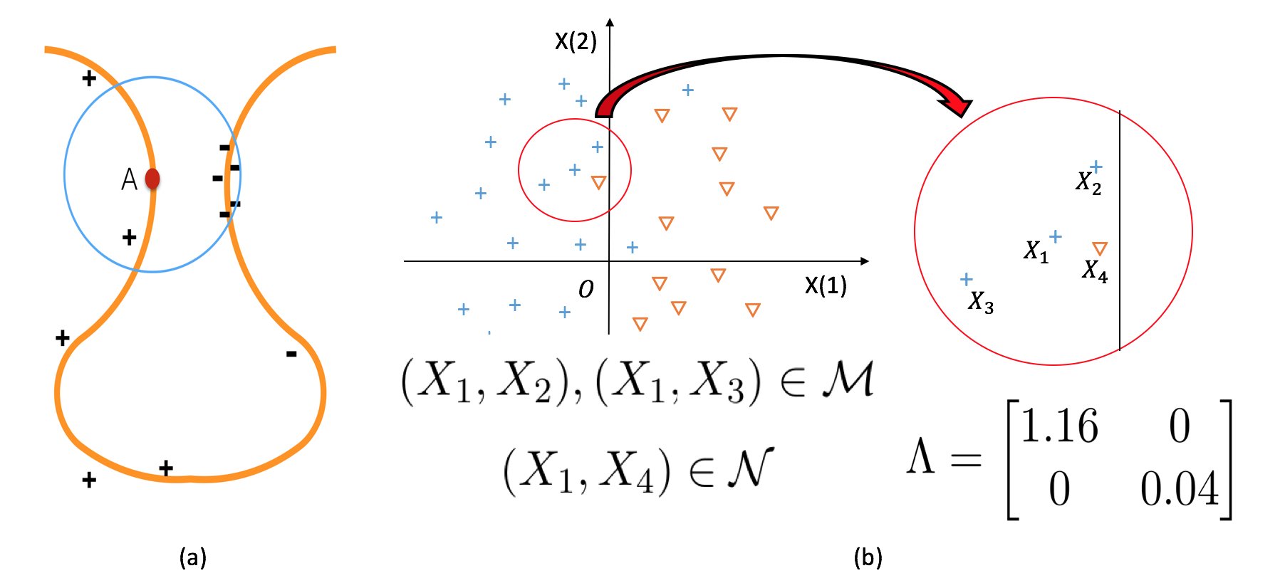
Figure 1. Stylized examples illustrating the need for data-driven cost function.

Figure 1(a) illustrates a classification task. The data roughly lies on a lower dimensional non-linear manifold. Some data which is classified with a negative label is seen to be “close” to data which is classified with a positive label when seeing the whole space (i.e. $\mathbb{R}^{2}$) as the natural ambient domain of the data. However, if we use a distance similar to the geodesic distance intrinsic to the manifold we would see that the negative instances are actually far from the positive instances. So, the generalization properties of the algorithm would be enhanced relative to using a standard metric in the ambient space, because with a given budget $\delta$ the adversarial player would be allowed perturbations mostly along the intrinsic manifold where the data lies and instances which are surrounded (in the intrinsic metric) by similarly classified examples will naturally carry significant impact in testing performance. A quantitative example to illustrate this point will be discussed in the sequel.

3. Background on Optimal Transport and Metric Learning Procedures

In this section we quickly review basic notions on optimal transport and metric learning methods so that we can define $D_{c}(P,P_{n})$ and explain how to calibrate the function $c(\cdot).$

3.1. Defining Optimal Transport Distances and Discrepancies

Assume that the cost function $c:\mathbb{R}^{d+1}\times\mathbb{R}^{d+1}\rightarrow[0,\infty]$ is lower semicontinuous. We also assume that $c(u,v)=0$ if and only if $u=v$. Given two distributions $P$ and $Q$, with supports $\mathcal{S}_{P}$ and $\mathcal{S}_{Q}$, respectively, we define the optimal transport discrepancy, $D_{c}$, via

(6) $$D_{c}\left(P,Q\right)=\inf\big{\{}\mathbb{E}_{\pi}\left[c(U,V)\right]:\pi\in\mathcal{P}\left(\mathcal{S}_{{}_{P}}\times\mathcal{S}_{{}_{Q}}\right),\text{ }\pi_{{}_{U}}=P,\text{ }\pi_{{}_{V}}=Q\big{\}},$$

where $\mathcal{P}(\mathcal{S}_{{}_{P}}\times\mathcal{S}_{{}_{Q}})$ is the set of probability distributions $\pi$ supported on $\mathcal{S}_{P}\times\mathcal{S}_{{}_{Q}}$, and $\pi_{{}_{U}}$ and $\pi_{{}_{V}}$ denote the marginals of $U$ and $V$ under $\pi$, respectively. Because $c(\cdot)$ is non-negative we have that $D_{c}(P,Q)\geq 0$. Moreover, requiring that $c(u,v)=0$ if and only if $u=v$ guarantees that $D_{c}(P,Q)=0$ if and only $P=Q$. If, in addition, $c(\cdot)$ is symmetric (i.e. $c(u,v)=c(v,u)$), and there exists $\varrho\geq 1$ such that $c^{1/\varrho}(u,w)\leq c^{1/\varrho}(u,v)+c^{1/\varrho}(v,w)$ (i.e. $c^{1/\varrho}(\cdot)$ satisfies the triangle inequality) then it can be easily verified (see Villani, (2008)) that $D_{c}^{1/\varrho}\left(P,Q\right)$ is a metric. For example, if $c(u,v)=\|u-v\|_{q}^{\varrho}$ for $q\geq 1$ (where $\|u-v\|_{q}$ denotes the $l_{q}$ norm in $\mathbb{R}^{d+1}$) then $D_{c}(\cdot)$ is known as the Wasserstein distance of order $\varrho$. Observe that (6) is a linear program in the variable $\pi.$

3.2. On Metric Learning Procedures

In order to keep the discussion focused, we use a few metric learning procedures, but we emphasize that our approach can be used in combination with virtually any method in the metric learning literature, see the survey paper Bellet et al., (2013) that contains additional discussion on metric learning procedures. The procedures that we consider, as we shall see, can be seen to already improve significantly upon natural benchmarks. Moreover, as we shall see, these metric families can be related to adaptive regularization. This connection will be useful to further enhance the intuition of our procedure.

3.2.1. The Mahalanobis Distance

The Mahalanobis metric is defined as

$$d_{\Lambda}\left(x,x^{\prime}\right)=\left(\left(x-x^{\prime}\right)^{T}\Lambda\left(x-x^{\prime}\right)\right)^{1/2},$$

where $\Lambda$ is symmetric and positive semi-definite and we write $\Lambda\in PSD$. Note that $d_{\Lambda}(x,x^{\prime})$ is the metric induced by the norm $\|x\|_{\Lambda}=\sqrt{x^{T}\Lambda x}$.
For a discussion, assume that our data is of the form $\mathcal{D}_{n}=\{(X_{i},Y_{i})\}_{i=1}^{n}$ and $Y_{i}\in\{-1,+1\}$. The prediction variables are assumed to be standardized. Motivated by applications such as social networks, in which there is a natural graph which can be used to connect instances in the data, we assume that one is given sets $\mathcal{M}$ and $\mathcal{N}$, where $\mathcal{M}$ is the set of the pairs that should be close (so that we can connect them) to each other, and $\mathcal{N}$, on contrary, is characterizing the relations that the pairs should be far away (not connected), we define them as

$$\mathcal{M}:=\left\{\left(X_{i},X_{j}\right)\text{ }|\text{ }X_{i}\text{ and }X_{j}\text{ must connect}\right\},\quad$$

$$\mathcal{N}:=\left\{\left(X_{i},X_{j}\right)\text{ }|\text{ }X_{i}\text{ and }X_{j}\text{ should not connect}\right\}.$$

While it is typically assumed that $\mathcal{M}$ and $\mathcal{N}$ are given, one may always resort to $k$-Nearest-Neighbor ($k$-NN) method for the generation of these sets. This is the approach that we follow in our numerical experiments. But we emphasize that choosing any criterion for the definition of $\mathcal{M}$ and $\mathcal{N}$ should be influenced by the learning task in order to retain both interpretability and performance.
In our experiments we let $\left(X_{i},X_{j}\right)$ belong to $\mathcal{M}$ if, in addition to being sufficiently close (i.e. in the $k$-NN criterion), $Y_{i}=Y_{j}$. If $Y_{i}\neq Y_{j}$, then we have that $\left(X_{i},X_{j}\right)\in\mathcal{N}$.
The work of Xing et al., (2002), one of the earlier reference on the subject, suggests considering

(7) $$\min_{\Lambda\in PSD} \sum_{\left(X_{i},X_{j}\right)\in\mathcal{M}}d_{\Lambda}^{2}\left(X_{i},X_{j}\right)$$

(8) $$\quad s.t. \quad\sum_{\left(X_{i},X_{j}\right)\in\mathcal{N}}d_{\Lambda}^{2}\left(X_{i},X_{j}\right)\geq\bar{\lambda}.$$

In words, the previous optimization problem minimizes the total distance between pairs that should be connect, while keeping the pairs that should not connect well separated. The constant $\bar{\lambda}>0$ is somewhat arbitrary (given that $\Lambda$ can be normalized by $\bar{\lambda}$, we can choose $\bar{\lambda}=1$).
The optimization problem (8) is an LP problem on the convex cone $PSD$ and it has been widely studied. Since $\Lambda\in PSD,$ we can always write $\Lambda=LL^{T}$, and therefore $d_{\Lambda}(X_{i},X_{j})=\left\|X_{i}-X_{j}\right\|_{\Lambda}:=\left\|LX_{i}-LX_{j}\right\|_{2}.$ There are various techniques which can be used to exploit the PSD structure to efficiently solve (8); see, for example, Xing et al., (2002) for a projection-based algorithm; or Schultz and Joachims, (2004), which uses a factorization-based procedure; or the survey paper Bellet et al., (2013) for the discussion of a wide range of techniques.
We have chosen formulation (8) to estimate $\Lambda$ because it is intuitive and easy to state, but the topic of learning Mahalanobis distances is an active area of research and there are different algorithms which can be implemented (see Li et al., (2016)).

3.2.2. Using Mahalanobis Distance in Data-Driven DRO

Let us assume that the underlying data takes the form $\mathcal{D}_{n}=\{(X_{i},Y_{i})\}_{i=1}^{n}$, where $X_{i}\in R^{d}$ and $Y_{i}\in R$ and the loss function, depending on a decision variable $\beta\in R^{m}$, is given by $l(x,y,\beta)$. Note that we are not imposing any linear structure on the underlying model or in the loss function. Then, motivated by the cost function (4), we may consider

(9) $$c_{{}_{\Lambda}}\big{(}(x,y),(x^{\prime},y^{\prime})\big{)}=d_{\Lambda}^{2}\left(x,x^{\prime}\right)I\left(y=y^{\prime}\right)+\infty I\left(y\neq y^{\prime}\right),$$

for $\Lambda\in PSD$. The infinite contribution in the definition of $c_{{}_{\Lambda}}$ (i.e. $\infty\cdot I\left(y\neq y^{\prime}\right)$) indicates that the adversarial player in the DRO formulation is not allowed to perturb the response variable.

Even in this case, since the definitions of $\mathcal{M}$ and $\mathcal{N}$ depend on $W_{i}=\left(X_{i},Y_{i}\right)$ (in particular, on the response variable), cost function $c_{{}_{\Lambda}}(\cdot)$ (once $\Lambda$ is calibrated using, for example, the method discussed in the previous subsection), will be informed by the $Y_{i}$s. Then, we estimate $\beta$ via

(10) $$\min_{\beta}\sup_{P:D_{c_{\Lambda}}\left(P,P_{n}\right)\leq\delta}\mathbb{E}[l(X,Y,\beta)].$$

It is important to note that $\Lambda$ has been applied only to the definition of the cost function.
The intuition behind the formulation can be gained in the context of a logistic regression setting, see the example in Figure 1(b): Suppose that $d=2$, and that $Y$ depends only on $X(1)$ (i.e. the first coordinate of $X$). Then, the metric learning procedure in (8) will induce a relatively low transportation cost across the $X(2)$ direction and a relatively high transportation cost in the $X(1)$ direction, whose contribution, being highly informative, is reasonably captured by the metric learning mechanism. Since the $X(1)$ direction is most impactful, from the standpoint of expected loss estimation, the adversarial player will reach a compromise, between transporting (which is relatively expensive) and increasing the expected loss (which is the adversary’s objective). Out of this compromise the DRO procedure localizes the out-of-sample enhancement, and yet improves generalization.

3.2.3. Mahalanobis Metrics on a Non-Linear Feature Space

In this section, we consider the case in which the cost function is defined after applying a non-linear transformation, $\Phi:R^{d}\rightarrow R^{l}$, to the data. Assume that the data takes the form $\mathcal{D}_{n}=\left\{\left(X_{i},Y_{i}\right)\right\}_{i=1}^{n}$, where $X_{i}\in\mathbb{R}^{d}$ and $Y_{i}\in\mathbb{R}$ and the loss function, depending on decision variable $\beta\in R^{m}$, is given by $l\left(x,y,\beta\right)$. Once again, motivated by the cost function (4), we may define

(11) $$c_{{}_{\Lambda}}^{\Phi}\big{(}(x,y),(x^{\prime},y^{\prime})\big{)}=d_{\Lambda}^{2}\left(\Phi\left(x\right),\Phi\left(x^{\prime}\right)\right)I\left(y=y^{\prime}\right)+\infty I\left(y\neq y^{\prime}\right),$$

for $\Lambda\in PSD$. To preserve the properties of a cost function (i.e. non-negativity, lower semicontinuity and $c_{\Lambda}^{\Phi}\left(u,w\right)=0$ implies $u=w$), we assume that $\Phi\left(\cdot\right)$ is continuous and that $\Phi\left(w\right)=\Phi\left(u\right)$ implies that $w=u$. Then we can apply a metric learning procedure, such as the one described in (8), to calibrate $\Lambda$. The intuition is the same as the one provided in the linear case in Section 3.2.2.

4. Data Driven Cost Selection and Adaptive Regularization

In this section we establish a direct connection between our fully data-driven DRO procedure and adaptive regularization. Moreover, our main result here, together with our discussion from the previous section, provides a direct connection between the metric learning literature and adaptive regularized estimators. As a consequence, the methods from the metric learning literature can be used to estimate the parameter of adaptively regularized estimators.
Throughout this section we consider again a data set of the form $\mathcal{D}_{n}=\left\{\left(X_{i},Y_{i}\right)\right\}_{i=1}^{n}$ with $X_{i}\in\mathbb{R}^{d}$ and $Y_{i}\in\mathbb{R}$. Motivated by the cost function (4) we define the cost function $c_{{}_{\Lambda}}(\cdot)$ as in (9). Using (9) we obtain the following result, which is proved in the appendix.

Theorem 1 (DRO Representation for Generalized Adaptive Regularization).

Assume that $\Lambda\in R^{d\times d}$ in (9) is positive definite. Given the data set $\mathcal{D}_{n}$, we obtain the following representation

(12) $$\min_{\beta}\max_{P:D_{c_{\Lambda}}\left(P,P_{n}\right)\leq\delta}\mathbb{E}_{P}^{1/2}\left[\left(Y-X^{T}\beta\right)^{2}\right]=\min_{\beta}\sqrt{\frac{1}{n}\sum_{i=1}^{n}\left(Y_{i}-X_{i}^{T}\beta\right)^{1/2}}+\sqrt{\delta}\left\|\beta\right\|_{\Lambda^{-1}}.$$

Moreover, if $Y\in\left\{-1,+1\right\}$ in the context of adaptive regularized logistic regression, we obtain the following representation

(13) $$\min_{\beta}\max_{P:D_{c_{\Lambda}}\left(P,P_{n}\right)\leq\delta}\mathbb{E}\left[\log\left(1+e^{-Y(X^{T}\beta)}\right)\right]=\min_{\beta}\frac{1}{n}\sum_{i=1}^{n}\log\left(1+e^{-Y_{i}(X_{i}^{T}\beta)}\right)+\delta\left\|\beta\right\|_{\Lambda^{-1}}.$$

In order to recover a more familiar setting in adaptive regularization, assume that $\Lambda$ is a diagonal positive definite matrix. In which case we obtain, in the setting of (12),

(14) $$\min_{\beta}\max_{P:D_{c_{\Lambda}}\left(P,P_{n}\right)\leq\delta}\mathbb{E}_{P}^{1/2}\left[\left(Y-X^{T}\beta\right)^{2}\right]=\min_{\beta}\sqrt{\frac{1}{n}\sum_{i=1}^{n}\left(Y_{i}-X_{i}^{T}\beta\right)^{2}}+\sqrt{\delta}\sqrt{\sum_{i=1}^{d}\beta_{i}^{2}/\Lambda_{ii}}.$$

The adaptive regularization method was first derived as a generalization for ridge regression in Hoerl and Kennard, 1970b () and Hoerl and Kennard, 1970a (). Recent work shows that adaptive regularization can improve the predictive power of its non-adaptive counterpart, specially in high-dimensional settings (see in Zou, (2006) and Ishwaran and Rao, (2014)).
In view of (14), our discussion in Section 3.2.1 uncovers tools which can be used to estimate the coefficients $\{1/\Lambda_{ii}:1<i\leq d\}$ using the connection to metric learning procedures. To complement the intuition given in Figure 1(b), note that in the adaptive regularization literature one often choose $\Lambda_{ii}\approx 0$ to induce $\beta_{i}\approx 0$ (i.e., there is a high penalty to variables with low explanatory power). This, in our setting, would correspond to transport costs which are low in such low explanatory directions.

5. Solving Data Driven DRO Based on Optimal Transport Discrepancies

In order to fully take advantage of the combination synergies between metric learning methodology and our DRO formulation, it is crucial to have a methodology which allows us to efficiently estimate $\beta$ in DRO problems such as (1). In the presence of a simplified representation such as (2) or (14), we can apply standard stochastic optimization results (see Lei and Jordan, (2016)).
Our objective in this section is to study algorithms which can be applied for more general loss and cost functions, for which a simplified representation might not be accessible.
Throughout this section, once again we assume that the data is given in the form $\mathcal{D}_{n}=\left\{\left(X_{i},Y_{i}\right)\right\}_{i=1}^{n}\subset\mathbb{R}^{d+1}$. The loss function is written as $\{l\left(x,y,\beta\right):\left(x,y\right)\in\mathbb{R}^{d+1},\beta\in\mathbb{R}^{m}\}$. We assume that for each $\left(x,y\right)$, the function $l\left(x,y,\cdot\right)$ is convex and continuously differentiable. Further, we shall consider cost functions of the form

$$\bar{c}\left(\left(x,y\right),\left(x^{\prime},y^{\prime}\right)\right)=c\left(x,x^{\prime}\right)I\left(y=y^{\prime}\right)+\infty I\left(y\neq y^{\prime}\right),$$

as this will simplify the form of the dual representation in the inner optimization of our DRO formulation. To ensure boundedness of our DRO formulation, we impose the following assumption.
Assumption 1. There exists $\Gamma(\beta,y)\in(0,\infty)$ such that $l(u,y,\beta)\leq\Gamma(\beta,y)\cdot(1+c(u,x)),$ for all $(x,y)\in\mathcal{D}_{n},$ Under Assumption 1, we can guarantee that

$$\max_{P:D_{c}\left(P,P_{n}\right)\leq\delta}\mathbb{E}_{P}\left[l\left(X,Y,\beta\right)\right]\leq\left(1+\delta\right)\max_{i=1,\ldots,n}\Gamma\left(\beta,Y_{i}\right)<\infty.$$

Using the strong duality theorem for semi-infinity linear programming problem in Appendix B of Blanchet et al., (2016),

(15) $$\max_{P:D_{c}\left(P,P_{n}\right)\leq\delta}\mathbb{E}_{P}\left[l\left(X,Y,\beta\right)\right]=\min_{\lambda\geq 0}\frac{1}{n}\sum_{i=1}^{n}\phi\left(X_{i},Y_{i},\beta,\lambda\right),$$

where $\psi(u,X,Y,\beta,\lambda):=l(u,Y,\beta)-\lambda(c(u,X)-\delta),$ $\phi\left(X,Y,\beta,\lambda\right):=\max_{u\in\mathbb{R}^{d}}\psi(u,X,Y,\beta,\lambda).$ Therefore,

(16) $$\min_{\beta}\max_{P:D_{c_{\Lambda}}\left(P,P_{n}\right)\leq\delta}\mathbb{E}_{P}\left[l\left(X,Y,\beta\right)\right]=\min_{\lambda\geq 0,\beta}\left\{\mathbb{E}_{P_{n}}\left[\phi\left(X,Y,\beta,\lambda\right)\right]\right\}.$$

The optimization in (16) is minimize over $\beta$ and $\lambda$, which we can consider stochastic approximation algorithm if the gradient of $\phi\left(\cdot\right)$ with respect to $\beta$ and $\lambda$ exist. However, $\phi\left(\cdot\right)$ is given in the form of the value function of a maximization problem, of which the gradient is not easy accessible. We will discuss the detailed algorithm and the validity of the smoothing approximation below.
We consider a smoothing approximation technique to remove the maximization problem $\phi\left(\cdot\right)$ using soft-max counterpart, $\phi_{\epsilon,f}\left(\cdot\right)$. The smoothing soft-max approximation has been explored and applied to approximately solve the DRO problem for the discrete case, where we restrict the distributionally uncertainty set only contains probability measures support on finite set (i.e., labeled training data and unlabeled training data with pseudo labels), we refer Blanchet and Kang, (2017) for further details.
However, due to the continuous-infinite support constraint, the soft-max approximation is a non-trivial generalization of the finite-discrete analogue. The smoothing approximation for $\phi\left(\cdot\right)$ is defined as,

$$\phi_{\epsilon,f}\left(X,Y,\beta,\lambda\right)=\epsilon\log\left(\int_{\mathbb{R}^{d}}\exp\left(\left[\psi\left(u,X,Y,\beta,\lambda\right)\right]/\epsilon\right)f\left(u\right)du\right),$$

where $f\left(\cdot\right)$ is a probability density in $\mathbb{R}^{d}$; for example, we can consider a multivariate normal distribution and $\epsilon$ is a small positive number regarded as smoothing parameter.
Theorem 2 below allows to quantify the error due to smoothing approximation.

Theorem 2.

Under mild technical assumptions (see Assumption 1-4 in Appendix B), there exists $\epsilon_{0}>0$ such that for every $\epsilon<\epsilon_{0}$, we have

$$\phi(X,Y,\beta,\lambda)\geq\phi_{\epsilon,f}(X,Y,\beta,\lambda)\geq\phi(X,Y,\beta,\lambda)-d\epsilon\log(1/\epsilon)$$

The proof of Theorem 2 is given in Appendix B.
After applying smooth approximation, the optimization problem turns into a standard stochastic optimization problem and we can apply mini-batch based stochastic approximation (SA) algorithm to solve it. As we can notice, as a function and $\beta$ and $\lambda$, the gradient of $\phi_{\epsilon,f}\left(\cdot\right)$ satisfies

$$\nabla_{\beta}\phi_{\epsilon,f}\left(X,Y,\beta,\lambda\right) =\frac{\mathbb{E}_{U\sim f}\left[\exp\left(\psi\left(U,X,Y,\beta,\lambda\right)/\epsilon\right)\nabla_{\beta}l\left(f_{\beta}\left(U\right),Y\right)\right]}{\mathbb{E}_{U\sim f}\left[\exp\left(\psi\left(U,X,Y,\beta,\lambda\right)/\epsilon\right)\right]},$$

$$\nabla_{\lambda}\phi_{\epsilon,f}\left(X,Y,\beta,\lambda\right) =\frac{\mathbb{E}_{U\sim f}\left[\exp\left(\psi\left(u,X,Y,\beta,\lambda\right)/\epsilon\right)\left(\delta-c_{\mathcal{D}_{n}}\left(u,X\right)\right)\right]}{\mathbb{E}_{U\sim f}\left[\exp\left(\psi\left(U,X,Y,\beta,\lambda\right)/\epsilon\right)\right]}.$$

However, since the gradients are still given in the form of expectation, we can apply a simple Monte Carlo sampling algorithm to approximate the gradient, i.e., we sample $U_{i}$’s from $f(\cdot)$ and evaluate the numerators and denominators of the gradient using Monte Carlo separately. For more details of the SA algorithm, please see in Algorithm 1.

Algorithm 1 Stochastic Gradient Descent with Continuous State

1:Initialize $\lambda=0$, and $\beta$ to be empirical risk minimizer, $\epsilon=0.5,$ tracking error $Error=100$.

2:while $Error>10^{-3}$ do

3:     Sample a mini-batch uniformly from observations $\left\{X_{(j)},Y_{(j)}\right\}_{j=1}^{M}$, with $M\leq n$.

4:     For each $j=1,\ldots,M$, sample i.i.d. $\{U_{k}^{(j)}\}_{k=1}^{L}$ from $\mathcal{N}\left(0,\sigma^{2}I_{d\times d}\right)$.

5:     We denote $f_{L}^{j}$ as empirical distribution for $U_{k}^{(j)}$’s, and estimate the batched as

$$\nabla_{\beta}\phi_{\epsilon,f}=\frac{1}{M}\sum_{j=1}^{M}\nabla_{\beta}\phi_{\epsilon,f_{L}^{j}}\left(X_{(j)},Y_{(j)},\beta,\lambda\right),\nabla_{\lambda}\phi_{\epsilon,f}=\frac{1}{M}\sum_{j=1}^{M}\nabla_{\lambda}\phi_{\epsilon,f_{L}^{j}}\left(X_{(j)},Y_{(j)},\beta,\lambda\right).$$

6:     Update $\beta$ and $\lambda$ using $\beta=\beta+\alpha_{\beta}\nabla_{\beta}\phi_{\epsilon,f}$ and $\lambda=\lambda+\alpha_{\lambda}\nabla_{\lambda}\phi_{\epsilon,f}.$

7:     Update tracking error $Error$ as the norm of difference between latest parameter and average of last $50$ iterations.

8:Output $\beta$.

6. Numerical Experiments

We validate our data-driven cost function based DRO using 5 real data examples from the UCI machine learning database Lichman, (2013). We focus on a DRO formulation based on the log-exponential loss for a linear model. We use the linear metric learning framework explained in equation (8), which then we feed into the cost function, $c_{\Lambda}$, as in (9), denoting by DRO-L. In addition, we also fit a cost function $c_{\Lambda}^{\Phi}$, as explained in (11) using linear and quadratric transformations of the data; the outcome is denote as (DRO-NL). We compare our DRO-L and DRO-NL with logistic regression (LR), and regularized logistic regression (LRL1). For each iteration and each data set, the data is split randomly into training and test sets. We fit the models on the training and evaluate the performance on test set. The regularization parameter is chosen via $5-$fold cross-validation for LRL1, DRO-L and DRO-NL. We report the mean and standard deviation for training and testing log-exponential error and testing accuracy for $200$ independent experiments for each data set. The details of the numerical results and basic information of the data is summarized in Table 1.

		BC	BN	QSAR	Magic	MB	SB
LR	Train	$0\pm 0$	$.008\pm.003$	$.026\pm.008$	$.213\pm.153$	$0\pm 0$	$0\pm 0$
	Test	$8.75\pm 4.75$	$2.80\pm 1.44$	$35.5\pm 12.8$	$17.8\pm 6.77$	$18.2\pm 10.0$	$14.5\pm 9.04$
	Accur	$.762\pm.061$	$.926\pm.048$	$.701\pm.040$	$.668\pm.042$	$.678\pm.059$	$.789\pm.035$
LRL1	Train	$.185\pm.123$	$.080\pm.030$	$.614\pm.038$	$.548\pm.087$	$.401\pm.167$	$.470\pm.040$
	Test	$.428\pm.338$	$.340\pm.228$	$.755\pm.019$	$.610\pm.050$	$.910\pm.131$	$.588\pm.140$
	Accur	$.929\pm.023$	$.930\pm.042$	$.646\pm.036$	$.665\pm.045$	$.717\pm.041$	$.811\pm.034$
DRO-L	Train	$.022\pm.019$	$.197\pm.112$	$.402\pm.039$	$.469\pm.064$	$.294\pm.046$	$.166\pm.031$
	Test	$.126\pm.034$	$.275\pm.093$	$.557\pm.023$	$.571\pm.043$	$.613\pm.053$	$.333\pm.018$
	Accur	$.954\pm.015$	$.919\pm.050$	$.733\pm.026$	$.727\pm.039$	$.714\pm.032$	$.887\pm.011$
DRO-NL	Train	$.032\pm.015$	$.113\pm.035$	$.339\pm.044$	$.381\pm.084$	$.287\pm.049$	$.195\pm.034$
	Test	$.119\pm.044$	$.194\pm.067$	$.554\pm.032$	$.576\pm.049$	$.607\pm.060$	$.332\pm.015$
	Accur	$.955\pm.016$	$.931\pm.036$	$.736\pm.027$	$.730\pm.043$	$.716\pm.054$	$.889\pm.009$
Num Predictors		$30$	$4$	$30$	$10$	$20$	$56$
Train Size		$40$	$20$	$80$	$30$	$30$	$150$
Test Size		$329$	$752$	$475$	$9990$	$125034$	$2951$

Table 1. Numerical results for real data sets.

7. Conclusion and Discussion

Our fully data-driven DRO procedure combines a semiparametric approach (i.e. the metric learning procedure) with a parametric procedure (expected loss minimization) to enhance the generalization performance of the underlying parametric model. We emphasize that our approach is applicable to any DRO formulation and is not restricted to classification tasks. An interesting research avenue that might be considered include the development of a semisupervised framework as in Blanchet and Kang, (2017), in which unlabeled data is used to inform the support of the elements in $\mathcal{U}_{\delta}(P_{n})$.

Appendix A Proof of Theorem 1

We first state and prove Lemma 1 which will be useful in proving Theorem 1.

Lemma 1.

If $\Lambda$ is a is positive definite matrix and we define $\left\|x\right\|_{\Lambda}=\left(x^{T}\Lambda x\right)^{1/2}$, then $\left\|\cdot\right\|_{\Lambda^{-1}}$ is the dual norm of $\left\|\cdot\right\|_{\Lambda}$. Furthermore, we have

$$u^{T}w\leq\left\|u\right\|_{\Lambda}\left\|w\right\|_{\Lambda^{-1}},$$

where the equality holds if and only if, there exists non-negative constant $\tau$, s.t $\tau\Lambda u=\Lambda^{-1}w$ or $\tau\Lambda^{-1}w=\Lambda u$.

Proof for Lemma 1.

This result is a direct generalization of $l_{2}$ norm in Euclidean space. Note that

(17) $$u^{T}w=\left(\Lambda u\right)^{T}(\Lambda^{-1}w)\leq\left\|\Lambda u\right\|_{2}\left\|\Lambda^{-1}w\right\|_{2}=\left\|u\right\|_{\Lambda}\left\|w\right\|_{\Lambda^{-1}}.$$

The inequality in the above is Cauchy-Schwartz inequality for $\mathbb{R}^{d}$ applies to $\Lambda u$ and $\Lambda^{-1}w$, and the equality holds if and only if there exists nonnegative $\tau$, s.t. $\tau\Lambda u=\Lambda^{-1}w$ or $\tau\Lambda^{-1}w=\Lambda u$. Now, by the definition of the dual norm,

$$\left\|w\right\|_{\Lambda}^{\ast}=\sup_{u:\left\|u\right\|_{\Lambda}\leq 1}u^{T}w=\sup_{u:\left\|u\right\|_{\Lambda}\leq 1}\left\|u\right\|_{\Lambda}\left\|w\right\|_{\Lambda^{-1}}=\left\|w\right\|_{\Lambda^{-1}}.$$

While the first equality follows from the definition of dual norm, the second equality is due to Cauchy-Schwartz inequality (17), and the equality condition therein, and the last equality are immediate after maximizing. ∎

Proof for Theorem 1.

The technique is a generalization of the method used in proving Theorem 1 in Blanchet et al., (2016). We can apply the strong duality result, see Proposition 6 in Appendix of Blanchet et al., (2016), for worst-case expected loss function, which is a semi-infinite linear programming problem, to obtain

$$\sup_{P:D_{c_{\Lambda}}\left(P,P_{n}\right)\leq\delta}\mathbb{E}_{P}\left[\left(Y-X^{T}\beta\right)^{2}\right]=\min_{\gamma\geq 0}\left\{\gamma\delta-\frac{1}{n}\sum_{i=1}^{n}\sup_{u}\left\{\left(y_{i}-u^{T}\beta\right)^{2}-\gamma\left\|x_{i}-u\right\|_{\Lambda}^{2}\right\}\right\}.$$

For the inner suprema , let us denote $\Delta=u-X_{i}$ and $e_{i}=Y_{i}-X_{i}^{T}\beta$ for notation simplicity. The inner optimization problem associated with $\left(X_{i},Y_{i}\right)$ becomes,

$$\sup_{u}\left\{\left(y_{i}-u^{T}\beta\right)^{2}-\gamma\left\|x_{i}-u\right\|_{\Lambda}^{2}\right\}$$

$$\quad=e_{i}^{2}+\sup_{\Delta}\left\{\left(\Delta^{T}\beta\right)^{2}-2e_{i}\Delta^{T}\beta-\gamma\left\|\Delta\right\|_{\Lambda}^{2}\right\},$$

$$\quad=e_{i}^{2}+\sup_{\Delta}\left\{\left(\sum_{j}\left|\Delta_{j}\right|\left|\beta_{j}\right|\right)^{2}+2\left|e_{i}\right|\sum_{j}\left|\Delta_{j}\right|\left|\beta_{j}\right|-\gamma\left\|\Delta\right\|_{\Lambda}^{2}\right\},$$

$$\quad=e_{i}^{2}+\sup_{\left\|\Delta\right\|_{\Lambda}}\left\{\left\|\Delta\right\|_{\Lambda}^{2}\left\|\beta\right\|_{\Lambda^{-1}}^{2}+2\left|e_{i}\right|\left\|\Delta\right\|_{\Lambda}\left\|\beta\right\|_{\Lambda^{-1}}-\gamma\left\|\Delta\right\|_{\Lambda}^{2}\right\},$$

$$\quad=\left\{\begin{array}[]{rcl}e_{i}^{2}\frac{\gamma}{\gamma-\left\|\beta\right\|_{\Lambda^{-1}}^{2}}&\text{ if }\gamma>\left\|\beta\right\|_{\Lambda^{-1}}^{2},&\\ +\infty\text{ }&\text{ if }\gamma\leq\left\|\beta\right\|_{\Lambda^{-1}}^{2}.&\end{array}\right.$$

While the first equality is due to the change of variable, the second equality is because we are working on a maximization problem, and the last term only depends on the magnitude rather than sign of $\Delta$, thus the optimization problem will always pick $\Delta$ that satisfying the equality. Considering the third equality, for the optimization problem, we can first apply the Cauchy-Schwartz inequality in Lemma 1 and we know that the maximization problem is to take $\Delta$ satisfying the equality constraint. For the last equality, if $\gamma\leq\left\|\beta\right\|_{\Lambda^{-1}}^{2}$, the optimization problem is unbounded, while $\gamma>\left\|\beta\right\|_{\Lambda^{-1}}^{2}$, we can solve the quadratic optimization problem and it leads to the final equality.

For the outer minimization problem over $\gamma$, as the inner suprema equal infinity if $\gamma\leq\left\|\beta\right\|_{\Lambda^{-1}}^{2}$, the worst-case expected loss becomes,

(18) $$\sup_{P:D_{c_{\mathcal{D}_{n}}}\left(P,P_{n}\right)\leq\delta}\mathbb{E}_{P}\left[\left(Y-X^{T}\beta\right)^{2}\right]$$

$$\quad=\min_{\gamma>\left\|\beta\right\|_{\alpha\text{-}(p,s)}^{2}}\left\{\gamma\delta-\frac{1}{n}\sum_{i=1}^{n}\left(Y_{i}-X_{i}^{T}\beta\right)\frac{\gamma}{\gamma-\left\|\beta\right\|_{\Lambda^{-1}}^{2}}\right\},$$

$$\quad=\left(\sqrt{\frac{1}{n}\sum_{i=1}^{n}\left(Y_{i}-X_{i}^{T}\beta\right)}+\sqrt{\delta}\left\|\beta\right\|_{\Lambda^{-1}}\right)^{2}.$$

The first equality follows the discussion above for restricting $\gamma>\left\|\beta\right\|_{\Lambda^{-1}}^{2}$. We can observe that the objective function in the right hand side of (18) is convex and differentiable and as $\gamma\rightarrow\infty$ and $\gamma\rightarrow\left\|\beta\right\|_{\Lambda}^{2}$, the value function will be infinity. We know the optimizer could be uniquely characterized via first order optimality condition. Solving for $\gamma$ in this way (through first order optimality), it is straightforward to obtain the last equality in (18). If we take square root on both sides, we prove the claim for linear regression.
For the log-exponential loss function, the proof follows a similar strategy. By applying strong duality results for semi-infinity linear programming problem in Blanchet et al., (2016), we can write the worst case expected loss function as,

$$\quad\sup_{P:D_{c_{\mathcal{D}_{n}}}\left(P,P_{n}\right)\leq\delta}\mathbb{E}_{P}\left[\log\left(1+\exp\left(-Y\beta^{T}X\right)\right)\right]$$

$$=\min_{\gamma\geq 0}\left\{\gamma\delta-\frac{1}{n}\sum_{i=1}^{n}\sup_{u}\left\{\log\left(1+\exp\left(-Y_{i}\beta^{T}u\right)\right)-\gamma\left\|X_{i}-u\right\|_{\Lambda}\right\}\right\}.$$

For each $i$, we can apply Lemma 1 in Shafieezadeh-Abadeh et al., (2015) and dual-norm result in Lemma 1 to deal with the inner optimization problem. It gives us,

$$\sup_{u}\left\{\log\left(1+\exp\left(-Y_{i}\beta^{T}u\right)\right)-\gamma\left\|X_{i}-u\right\|_{\Lambda}\right\}=\left\{\begin{array}[]{ccc}\log\left(1+\exp\left(-Y_{i}\beta^{T}X_{i}\right)\right)&\text{if}&\left\|\beta\right\|_{\Lambda^{-1}}\leq\gamma,\\ \infty&\text{if}&\left\|\beta\right\|_{\Lambda^{-1}}>\gamma.\end{array}\right.$$

Moreover, since the outer optimization is trying to minimize, following the same discussion for the proof for linear regression case, we can plug-in the result above and it leads the first equality below,

$$\min_{\gamma\geq 0}\left\{\gamma\delta-\frac{1}{n}\sum_{i=1}^{n}\sup_{u}\left\{\log\left(1+\exp\left(-Y_{i}\beta^{T}u\right)\right)-\gamma\left\|X_{i}-u\right\|_{\Lambda}\right\}\right\}$$

$$\quad=\min_{\gamma\geq\left\|\beta\right\|_{\Lambda^{-1}}}\left\{\delta\gamma+\frac{1}{n}\sum_{i=1}^{n}\log\left(1+\exp\left(-Y_{i}\beta^{T}X_{i}\right)\right)\right\}$$

$$\quad=\frac{1}{n}\sum_{i=1}^{n}\log\left(1+\exp\left(-Y_{i}\beta^{T}X_{i}\right)\right)+\delta\left\|\beta\right\|_{\Lambda^{-1}}.$$

We know that the target function is continuous and monotone increasing in $\gamma$, thus we can notice it is optimized by taking $\gamma=\left\|\beta\right\|_{\Lambda^{-1}}$, which leads to second equality above. This proves the claim for logistic regression in the statement of the theorem. ∎

Appendix B Proof of Theorem 2

Let us begin by listing the assumptions required to prove Theorem 2. First, we begin by recalling Assumption 1 from Section 5.

Assumption 1. There exists $\Gamma(\beta,y)\in(0,\infty)$ such that $l(u,y,\beta)\leq\Gamma(\beta,y)\cdot(1+c(u,x)),$ for all $(x,y)\in\mathcal{D}_{n},$

We now introduce Assumptions 2-4 below.

Assumption 2. $\psi\left(\cdot,X,Y,\beta,\lambda\right)$ is twice continuously differentiable and the Hessian of $\psi\left(\cdot,X,Y,\beta,\lambda\right)$ evaluated at $u^{\ast}$, $D_{u}^{2}\psi\left(u^{\ast},X,Y,\beta,\lambda\right)$, is positive definite. In particular, we can find $\theta>0$ and $\eta>0$, such that

$$\psi(u,X,Y,\beta,\lambda)\geq\psi\left(u^{\ast},X,Y,\beta,\lambda\right)-\frac{\theta}{2}\|u-u^{\ast}\|_{2}^{2},\quad\forall u\text{ with }\left\|u-u^{\ast}\right\|_{2}\leq\eta.$$

Assumption 3. For a constant $\lambda_{0}>0$ such that $\phi(X,Y,\beta,\lambda_{0})<\infty$, let $K=K\left(X,Y,\beta,\lambda_{0}\right)$ be any upper bound for $\phi(X,Y,\beta,\lambda_{0})$.

Assumption 4. In addition to the lower semicontinuity of $c\left(\cdot\right)\geq 0$, we assume that $c\left(\cdot,X\right)$ is coercive in the sense that $c\left(u,X\right)\rightarrow\infty$ as $\left\|u\right\|_{2}\rightarrow\infty$.

For any set $S$, the $r$-neighborhood of $S$ is defined as the set of all points in $\mathbb{R}^{d}$ that are at distance less than $r$ from $S$, i.e. $S_{r}=\cup_{u\in S}\{\bar{u}:\left\|\bar{u}-u\right\|_{2}\leq r\}$.

Proof of Theorem 2.

The first part of the inequality is easy to derive. For the second part, we proceed as follows: Under Assumptions 3 and 4, we can define the compact set

$$\mathcal{C}=\mathcal{C}(X,Y,\beta,\lambda)=\{u:c(u,X)\leq l(X,Y,\beta)-K+\lambda_{0}/(\lambda-\lambda_{0})\}.$$

It is easy to check that $\arg\max\{\psi\left(u,X,Y,\lambda\right)\}\subset\mathcal{C}$. Owing to optimality of $u^{\ast}$ and from Assumption 2 that $K\geq\phi(X,Y,\beta,\lambda_{0})$, we can see that

$$l(X,Y) \leq l(u^{\ast},Y))-\lambda c(u,X)$$

$$=l(u^{\ast},Y)-\lambda_{0}c(u^{\ast},X)-(\lambda-\lambda_{0})c(u^{\ast},X)$$

$$\leq K-\lambda_{0}-(\lambda-\lambda_{0})c(u^{\ast},X).$$

Thus by definition of $\mathcal{C}=\mathcal{C}(X,Y,\beta,\lambda)$, it follows easily that $u^{\ast}\in\mathcal{C}$, which further implies $\{u:\|u-u^{\ast}\|_{2}\leq\eta\}\subset\mathcal{C}_{\eta}$. Then we combine the strongly convexity assumption in Assumption 2 and the definition of $\phi_{\epsilon,f}(u,X,Y,\beta,\lambda)$, which yields

$$\phi_{\epsilon,f}\left(X,Y,\beta,\lambda\right) \geq\epsilon\log\left(\int_{\|u-u^{\ast}\|_{2}\leq\eta}\exp\left(\left[\phi\left(X,Y,\beta,\lambda\right)-\frac{\theta}{2}\|u-u^{\ast}\|_{2}^{2}\right]/\epsilon\right)f(u)du\right)$$

$$=\epsilon\log\left(\exp\left(\phi\left(X,Y,\beta,\lambda\right)/\epsilon\right)\right)\int_{\|u-u^{\ast}\|_{2}\leq\eta}\exp\left(-\frac{\theta}{2}\|u-u^{\ast}\|_{2}^{2}/\epsilon\right)f(u)du$$

$$=\phi\left(X,Y,\beta,\lambda\right)+\epsilon\log\int_{\|u-u^{\ast}\|_{2}\leq\eta}\exp\left(-\frac{\theta\|u-u^{\ast}\|_{2}^{2}}{2\epsilon}\right)f(u)du.$$

As $\{u:\|u-u^{\ast}\|_{2}\leq\eta\}\subset\mathcal{C}_{\eta}$, we can use the lower bound of $f(\cdot)$ to deduce that

$$\int_{\|u-u^{\ast}\|_{2}\leq\eta}\exp\left(-\frac{\theta\|u-u^{\ast}\|_{2}^{2}}{2\epsilon}\right)f(u)du \geq\inf_{u\in\mathcal{C}_{\eta}}f(u)\times\int_{\|u-u^{\ast}\|_{2}\leq\eta}\exp\left(-\frac{\theta\|u-u^{\ast}\|_{2}^{2}}{2\epsilon}\right)du$$

$$=\inf_{u\in\mathcal{C}_{\eta}}f(u)\times\left(2\pi\epsilon/\theta\right)^{d/2}P(Z_{d}\leq\eta^{2}\theta/\epsilon),$$

where $Z_{d}$ is a chi-squared random variable of $d$ degrees of freedom. To conclude, recall that $\epsilon\in(0,\eta^{2}\theta\chi_{\alpha})$, the lower bound of $\phi_{\epsilon,f}(\cdot)$ can be written as

$$\phi_{\epsilon,f}(X,Y,\beta,\lambda)\geq\phi(X,Y,\beta,\lambda)-\frac{d}{2}\epsilon\log(1/\epsilon)+\frac{d}{2}\epsilon\log\left(\left(2\pi\alpha/\theta\right)\inf_{u\in\mathcal{C}_{\eta}}f(u)\right).$$

This completes the proof of Theorem 2. ∎

References

- Bellet et al., [2013] Bellet, A., Habrard, A., and Sebban, M. (2013). A survey on metric learning for feature vectors and structured data. arXiv preprint arXiv:1306.6709.
- Blanchet and Kang, [2017] Blanchet, J. and Kang, Y. (2017). Distributionally robust semi-supervised learning. arXiv preprint arXiv:1702.08848.
- Blanchet et al., [2016] Blanchet, J., Kang, Y., and Murthy, K. (2016). Robust wasserstein profile inference and applications to machine learning. arXiv preprint arXiv:1610.05627.
- Esfahani and Kuhn, [2015] Esfahani, P. M. and Kuhn, D. (2015). Data-driven distributionally robust optimization using the wasserstein metric: Performance guarantees and tractable reformulations. arXiv preprint arXiv:1505.05116.
- Friedman et al., [2001] Friedman, J., Hastie, T., and Tibshirani, R. (2001). The elements of statistical learning, volume 1. Springer series in statistics Springer, Berlin.
- [6] Hoerl, A. E. and Kennard, R. W. (1970a). Ridge regression: applications to nonorthogonal problems. Technometrics, 12(1):69–82.
- [7] Hoerl, A. E. and Kennard, R. W. (1970b). Ridge regression: Biased estimation for nonorthogonal problems. Technometrics, 12(1):55–67.
- Hu and Hong, [2013] Hu, Z. and Hong, L. J. (2013). Kullback-leibler divergence constrained distributionally robust optimization. Available at Optimization Online.
- Ishwaran and Rao, [2014] Ishwaran, H. and Rao, J. S. (2014). Geometry and properties of generalized ridge regression in high dimensions. Contemp. Math, 622:81–93.
- Lei and Jordan, [2016] Lei, L. and Jordan, M. I. (2016). Less than a single pass: Stochastically controlled stochastic gradient method. arXiv preprint arXiv:1609.03261.
- Li et al., [2016] Li, L., Sun, C., Lin, L., Li, J., and Jiang, S. (2016). A mahalanobis metric learning-based polynomial kernel for classification of hyperspectral images. Neural Computing and Applications, pages 1–11.
- Lichman, [2013] Lichman, M. (2013). UCI machine learning repository.
- Schultz and Joachims, [2004] Schultz, M. and Joachims, T. (2004). Learning a distance metric from relative comparisons. In Advances in neural information processing systems, pages 41–48.
- Shafieezadeh-Abadeh et al., [2015] Shafieezadeh-Abadeh, S., Esfahani, P. M., and Kuhn, D. (2015). Distributionally robust logistic regression. In Advances in Neural Information Processing Systems, pages 1576–1584.
- Villani, [2008] Villani, C. (2008). Optimal transport: old and new, volume 338. Springer Science & Business Media.
- Xing et al., [2002] Xing, E. P., Ng, A. Y., Jordan, M. I., and Russell, S. (2002). Distance metric learning with application to clustering with side-information. In NIPS, volume 15, page 12.
- Zou, [2006] Zou, H. (2006). The adaptive lasso and its oracle properties. Journal of the American statistical association, 101(476):1418–1429.