Simultaneous Multiple Surface Segmentation Using Deep Learning

Abstract

The task of automatically segmenting 3-D surfaces representing boundaries of objects is important for quantitative analysis of volumetric images, and plays a vital role in biomedical image analysis. Recently, graph-based methods with a global optimization property have been developed and optimized for various medical imaging applications. Despite their widespread use, these require human experts to design transformations, image features, surface smoothness priors, and re-design for a different tissue, organ or imaging modality. Here, we propose a Deep Learning based approach for segmentation of the surfaces in volumetric medical images, by learning the essential features and transformations from training data, without any human expert intervention. We employ a regional approach to learn the local surface profiles. The proposed approach was evaluated on simultaneous intraretinal layer segmentation of optical coherence tomography (OCT) images of normal retinas and retinas affected by age related macular degeneration (AMD). The proposed approach was validated on 40 retina OCT volumes including 20 normal and 20 AMD subjects. The experiments showed statistically significant improvement in accuracy for our approach compared to state-of-the-art graph based optimal surface segmentation with convex priors (G-OSC). A single Convolution Neural Network (CNN) was used to learn the surfaces for both normal and diseased images. The mean unsigned surface positioning errors obtained by G-OSC method $2.31$ voxels ($95\%$ CI $2.02$-$2.60$ voxels) was improved to $1.27$ voxels ($95\%$ CI $1.14$-$1.40$ voxels) using our new approach. On average, our approach takes $94.34$ s, requiring 95.35 MB memory, which is much faster than the $2837.46$ s and 6.87 GB memory required by the G-OSC method on the same computer system.

1 Introduction

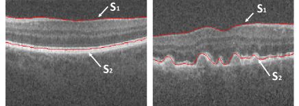
For the diagnosis and management of disease, segmentation of images of organs and tissues is a crucial step for the quantification of medical images. Segmentation finds the boundaries or, limited to the 3-D case, the surfaces, that separate organs, tissues or regions of interest in an image. Current state-of-the-art methods for automated 3-D surface segmentation use expert designed graph search / graph cut approaches [5] or active shape/contour modelling [8], all based on classical expert designed image properties, using carefully designed transformations including mathematical morphology and wavelet transformations. For instance, OCT is a 3-D imaging technique that is widely used in the diagnosis and management of patients with retinal diseases. The tissue boundaries in OCTs vary by presence and severity of disease. An example is shown in Fig.1(a)(b) to illustrate the difference in profile for the Internal Limiting Membrane (ILM) and Inner Retinal Pigment Epithelium (IRPE) in a normal eye and in an eye with AMD. In order to overcome these different manifesttaions, graph based methods [5][6][7] with transformations, smoothness constraints, region of interest extraction and multiple resolution approaches designed by experts specifically for the target surface profile have been used. The contour modelling approach [8] requires surface specific and expert designed region based and shape prior terms. The current methods for surface segmentation in OCTs are highly dependent on expert designed target surface specific transformations and therefore, there is a desire for approaches which do not require human expert intervention. Deep learning, where all transformation levels are determined from training data, instead of being designed by experts, has been highly successful in a large number of computer vision [4] and medical image analysis detection tasks [1][3], substantially outperforming all classical image analysis techniques, and given the spatial coherence that is characteristic of images, typically implemented as Convolutional Neural Networks (CNN) [4]. All these examples are where CNNs are used to identify pixels or voxels as belonging to a certain class, called classification and not to identify boundaries in the images, i.e. segmentation.

In this study, we propose a CNN based deep learning approach for boundary surface segmentation of a target object, where both features and models are learnt from training data without intervention by a human expert. We are particularly interested in terrain-like surfaces. An image volume is generally represented as a 3-D volumetric cube consisting of voxel columns, wherein a terrain-like surface intersects each column at exactly one single voxel location. The smoothness of a given surface may be interpreted as the piecewise change in the surface positions of two neighboring columns. The graph based optimal surface segmentation methods [5][7] use convex functions to impose the piecewise smoothness while globally minimizing the objective function for segmentation. In order to employ CNNs for surface segmentation, two key questions need to be answered. First, since most of the CNN based methods have been used for classification, how can a boundary be segmented using a CNN? Second, how can the CNN learn the surface smoothness and surface distance between two interacting surfaces implicitly? We answer these questions by representing consecutive target surface positions for a given input image as a vector. For example, $m_{1}$ consecutive target surface positions for a single surface are represented as a $m_{1}$-D vector, which may be interpreted as a point in the $m_{1}$-D space, while maintaining a strict order with respect to the consecutiveness of the target surface positions. The ordering of the target surface positions partially encapsulates the smoothness of the surface. Thereafter, the error (loss) function utilized in the CNN to back propagate the error is chosen as a Euclidean loss function shown in Equation (1), wherein the network adjusts the weights of the various nonlinear transformations within the network to minimize the Euclidean distance between the CNN output and the target surface positions in the $m_{1}$-D space. Similarly, for detecting $\lambda$ surfaces, the surface positions are represented as a $m_{2}$-D vector, where $\lambda=\{1,2,\ldots\lambda\}$, $m_{2}=\lambda\times m_{1}$ and $m_{1}$ consecutive surface poistions for a surface index $i$ ($i\in\lambda$) are given by $\{((i-1)\times m_{1})+1,((i-1)\times m_{1})+2,\ldots((i-1)\times m_{1})+m_{1}\}$ index elements in the $m_{2}$-D vector.

Figure 1: Illustration of difference in surface profiles on a single B-scan. (left) Normal Eye (right) Eye with AMD. $S_{1}$ = ILM and $S_{2}$ = IRPE, are shown in red.

In the currently used methods for segmentation of surfaces, the surface smoothness is piecewise in nature. The surface smoothness penalty (cost) enforced in these methods is the sum of the surface smoothness penalty ascertained using the difference of two consecutive surface positions. Thus, such methods require an expert designed, and application specific, smoothness term to attain accurate segmentations. On the contrary, segmentation using CNN should be expected to also learn the different smoothness profiles of the target surface. Because the smoothness is piecewise, it should be sufficient for the CNN to learn the different local surface profiles for individual segments of the surface with high accuracy because the resultant surface is a combination of these segments. Hence, the CNN is trained on individual patches of the image with segments of the target surface.

2 Method

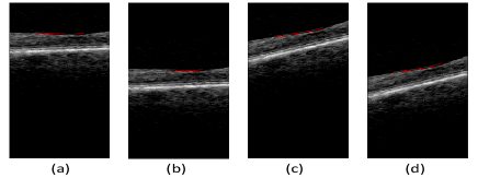
Consider a volumetric image $I(x,y,z)$ of size $X\times Y\times Z$. A surface is defined as $S(x,y)$, where $x\in{\bf x}$ = $\{0,1,...X-1\}$, $y\in{\bf y}$ =$\{0,1,...Y-1\}$ and $S(x,y)\in{\bf z}$ = $\{0,1,...Z-1\}$. Each $(x,y)$ pair forms a voxel column parallel to the z-axis, wherein the surface $S(x,y)$ intersects each column at a single voxel location. For simlutaneously segmenting $\lambda(\lambda\geq 2)$ surfaces, the goal of the CNN is to learn the surface positions $S_{i}(x,y)$ ($i\in\lambda$) for columns formed by each $(x,y)$ pair. In this work, we present a slice by slice segmentation of a 3-D volumetric image applied on OCT volumes. Patches are extracted from B-scans with the target Reference Standard (RS). A patch $P(x_{1},z)$ is of size $N\times Z$, where $x_{1}\in{\bf x_{1}}$ = $\{0,1,...N-1\}$, $z\in{\bf z}$ =$\{0,1,...Z-1\}$ and $N$ is a multiple of $4$. The target surfaces $S_{i}$’s to be learnt simultaneously from $P$ is $\overline{S_{i}}(x_{2})\in{\bf z}$ = $\{0,1,...Z-1\}$, where $x_{2}\in{\bf x_{2}}$ = $\{\frac{N}{4},\frac{N}{4}+1...\frac{3N}{4}-1\}$. Essentially, the target surfaces to be learnt is the surface locations for the middle $\frac{N}{2}$ consecutive columns in $P$. The overlap between consecutive patches ensures no abrupt changes occur at patch boundaries. By segmenting the middle $N/2$ columns in a patch size with $N$ columns, the boundary of patches overlap with the consecutive surface segment patch. Then, data augmentation is performed, where for each training patch, three additional training patches were created. First, a random translation value was chosen between -250 and 250 such that the translation was within the range of the patch size. The training patch and the corresponding RS for surfaces $\overline{S_{i}}$’s were translated in the $z$ dimension accordingly. Second, a random rotation value was chosen between -45 degrees and 45 degrees. The training patch and the corresponding RS for surfaces $\overline{S_{i}}$’s were rotated accordingly. Last, a combination of rotation and translation was used to generate another patch. Examples of data augmentation on patches for a single surface is shown in Fig.2.

Figure 2: Illustration of data augmentation applied to an input patch. The target surface is shown in red. (a)Extracted patch from a B-scan, (b)Translation (c)Rotation (d)Translation and rotation, as applied to (a).

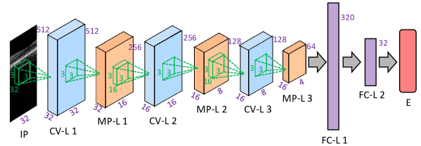
For segmenting $\lambda$ surfaces simultaneously, the CNN learns $\lambda$ surfaces for each patch. The CNN architecture used in our work is shown in Fig.3, employed for $\lambda=2$ and patches with $N=32$. The CNN contains three convolution layers [4], each of which is followed by a max-pooling layer [4] with stride length of two. Thereafter, it is followed by two fully connected layers [4], where the last fully connected layer represents the final output of the middle $\frac{N}{2}$ surface positions for 2 target surfaces in $P$. Lastly, a Euclidean loss function (used for regressing to real-valued labels) as shown in Equation (1) is utilized to compute the error between CNN outputs and RS of $S_{i}$’s ($i\in\lambda$) within $P$ for back propagation during the training phase. Unsigned mean surface positioning error (UMSPE) [5] is one of the commonly used error metric for evaluation of surface segmentation accuracy. The Euclidean loss function (E), essentially computes sum of the squared unsigned surface positioning error over the $\frac{N}{2}$ consecutive surface position for $S_{i}$’s of the CNN output and the RS for $P$.

Figure 3: The architecture of the CNN learned in our work for $N$=$32$ and $\lambda=2$. The numbers along each side of the cuboid indicate the dimensions of the feature maps. The inside cuboid ($green$) represents the convolution kernel and the inside square ($green$) represents the pooling region size. The number of hidden neurons in the fully connected layers are marked aside. IP=Input Patch, CV-L=Convolution Layer, MP-L=Max-Pooling Layer, FC-L=Fully Connected Layer, E=Euclidean Loss Layer.

$$E=\sum_{i=1}^{i=\lambda}\sum_{k_{1}=0}^{k_{1}=\frac{N}{2}-1}(\overline{a}^{i}_{k_{1}}-a^{i}_{k_{2}})^{2}$$ (1)

where $k_{2}=((i-1)\times N/2)+k_{1}$, $\overline{a}^{i}_{k_{1}}$ and ${a}^{i}_{k_{2}}$ is the $k_{1}$-$th$ surface position of reference standard and CNN output respectively for surface $S_{i}$ in a given $P$.

3 Experiments

The experiments compare segmentation accuracy of the proposed CNN based method (CNN-S) and G-OSC method [7]. The two surfaces simultaneously segmented in this study are $S_{1}$-ILM and $S_{2}$-IRPE as shown in Fig. 1. $115$ OCT scans of normal eyes, $269$ OCT scans of eyes with AMD and their respective reference standards (RS) (created by experts with aid of the DOCTRAP software [2]) were obtained from the publicly available repository [2]. The 3-D volume size was $1000\times 100\times 512$ voxels. The data volumes were divided into a training set ($79$ normal and $187$ AMD), a testing set ($16$ normal and $62$ AMD) and a validation set ($20$ normal and $20$ AMD). The volumes were denoised by applying a median filter of size $5\times 5\times 5$ and normalized with the resultant voxel intensity varying from -1 to 1. Thereafter, patches of size $N\times 512$ with their respective RS for the middle $\frac{N}{2}$ consecutive surface positions for $S_{1}$ and $S_{2}$ is extracted using data augmentation, for training and testing volumes, resulting in a training set of $340,000$ and testing set of $70,000$ patches. In our work, we use $N=32$. The UMSPE was used to evaluate the accuracy. The complete surfaces for each validation volume were segmented using the CNN-S method by creating $\frac{1016}{N/2}$ patches from each B-scan where each B-scan was zero padded with $8$ voxel columns at each extremity. Statistical significance of observed differences was determined by paired Student $t$-tests for which $p$ value of 0.05 was considered significant. In our study we used one NVIDIA Titan X GPU for training the CNN. The validation using the G-OSC and CNN-S method were carried out on a on a Linux workstation (3.4 GHz, 16 GB memory). A single CNN was trained to infer on both the normal and AMD OCT scans. For a comprehensive comparison, three experiments were performed with the G-OSC method. The first experiment (G-OSC $1$) involved segmenting the surfaces in both normal and AMD OCT scans using a same set of optimized parameters. The second (G-OSC $2$) and third (G-OSC $3$) experiment involved segmenting the normal and AMD OCT scans with different set of optimized parameters, respectively.

4 Results

The quantitative comparisons between the proposed CNN-S method and the G-OSC method on the validation volumes is summarized in Table 1. For the entire validation data, the proposed method produced significantly lower UMSPE for surfaces $S_{1}$ ($p<0.01$) and $S_{2}$ ($p<0.01$), compared to the segmentation results of G-OSC $1$, G-OSC $2$ and G-OSC $3$. Illustrative results of segmentations from the CNN-S, G-OSC $2$ and G-OSC $3$ methods on validation volumes are shown in Fig. 4. It can be observed that CNN-S method yeilds consistent and qualitatively superior segmentations with respect to the G-OSC method. On closer analysis of some B-scans in the validation data, the CNN-S method produced high quality segmentation for a few cases where the RS was not accurate enough as verifed by an expert (4th row in Fig. 4). The CNN required $17$ days to train on the GPU. The CNN-S method with average computation time of 94.34 seconds (95.35 MB memory) is much faster than G-OSC with average computation time of 2837.46 seconds (6.87 GB memory).

Table 1: UMSPE expressed as (mean $\pm$ $95\%$ CI) in voxels. RS - Reference Standard. $N=32$ was used as the patch size ($32\times 512$).

	Normal and AMD		Normal		AMD
	G-OSC 1	CNN-S	G-OSC 2	CNN-S	G-OSC 3	CNN-S
Surface	vs. RS	vs. RS	vs. RS	vs. RS	vs. RS	vs.RS
$S_{1}$	1.45 $\pm$ 0.19	0.98 $\pm$ 0.08	1.19 $\pm$ 0.05	0.89 $\pm$ 0.07	1.37 $\pm$ 0.22	1.06 $\pm$ 0.11
$S_{2}$	3.17 $\pm$ 0.43	1.56 $\pm$ 0.15	1.41 $\pm$ 0.11	1.28 $\pm$ 0.10	2.88 $\pm$ 0.54	1.83 $\pm$ 0.26
Overall	2.31 $\pm$ 0.29	1.27 $\pm$ 0.13	1.31 $\pm$ 0.07	1.08 $\pm$ 0.08	2.13 $\pm$ 0.39	1.44 $\pm$ 0.19

Figure 4: Each row shows the same B-scan from a Normal or AMD OCT volume. (a) CNN-S vs. RS (b) G-OSC vs. RS, for surfaces $S_{1}$ =ILM and $S_{2}$ = IRPE. RS = Reference Standard, Red = reference standard, Green = Segmentation using proposed method and Blue = Segmentation using G-OSC method. In the 4th row, we had the reference standard reviewed by a fellow-ship trained retinal specialist, who stated that the CNN-S method is closer to the real surface than the reference standard.

5 Discussion and Conclusion

The results demonstrate superior quality of segmentations compared to the G-OSC method, while eliminating the requirement of expert designed transforms. The proposed method used a single CNN to learn various local surface profiles for both normal and AMD data. Our results compared to G-OSC $1$ show that the CNN-S methods outperforms the G-OSC method. If the parameters are tuned specifically for each type of data by using expert prior knowledge while using the G-OSC method, as in the cases of G-OSC $2$ and G-OSC $3$, the results depict that the CNN-S method still results in superior performance. The inference using CNN-S is much faster than G-OSC method and requires much less memory. Consequently, the inference can be parallelized for multiple patches, thereby further reducing the computation time, thus making it potentially more suitable for clinical applications. However, a drawback of any such learning approach in medical imaging is the limited amount of available training data. The proposed method was trained on images from one type of scanner and hence it is possible that the trained CNN may not produce consistent segmetnations on images obtained from a different scanner due to difference in textural and spatial information. The approach can readily be extended to perform 3-D segmentations by employing 3-D convolutions.

In this paper, we proposed a CNN based method for segmentation of surfaces in volumetric images with implicitly learned surface smoothness and surface separation models. We demonstrated the performance and potential of the proposed method through application on OCT volumes to segment the ILM and IRPE surface. The experiment results show higher segmentation accuracy as compared to the G-OSC method. To the best of our knowledge, this is the first method of its kind that does not require any human intervention for surface segmentation.

References

- [1] Challenge, M.B.G.: Multimodal brain tumor segmentation benchmark: Change detection. http://braintumorsegmentation.org/, accessed November 5, 2016
- [2] Farsiu, S., Chiu, S.J., O’Connell, R.V., Folgar, F.A., Yuan, E., Izatt, J.A., Toth, C.A.: Quantitative classification of eyes with and without intermediate age-related macular degeneration using optical coherence tomography. Ophthalmology 121(1), 162–172 (2014)
- [3] Kaggle: Diabetic retinopathy detection. http://www.kaggle.com/c/diabetic-retinopathy-detection/, accessed July 15, 2016
- [4] Krizhevsky, A., Sutskever, I., Hinton, G.E.: Imagenet classification with deep convolutional neural networks. In: Advances in neural information processing systems. pp. 1097–1105 (2012)
- [5] Lee, K., Garvin, M., Russell, S., Sonka, M., Abràmoff, M.: Automated intraretinal layer segmentation of 3-d macular oct scans using a multiscale graph search. Investigative Ophthalmology & Visual Science 51(13), 1767–1767 (2010)
- [6] Shah, A., Bai, J., Hu, Z., Sadda, S., Wu, X.: Multiple surface segmentation using truncated convex priors. In: Medical Image Computing and Computer-Assisted Intervention–MICCAI 2015, pp. 97–104. Springer (2015)
- [7] Song, Q., Bai, J., Garvin, M.K., Sonka, M., Buatti, J.M., Wu, X.: Optimal multiple surface segmentation with shape and context priors. Medical Imaging, IEEE Transactions on 32(2), 376–386 (2013)
- [8] Yazdanpanah, A., Hamarneh, G., Smith, B., Sarunic, M.: Intra-retinal layer segmentation in optical coherence tomography using an active contour approach. In: International Conference on Medical Image Computing and Computer-Assisted Intervention. pp. 649–656. Springer (2009)