Wealth dynamics in a sentiment-driven market

Abstract

We study dynamics of a simulated world with stock and money, driven by the externally given processes which we refer to as sentiments. The considered sentiments influence the buy/sell stock trading attitude, the perceived price uncertainty, and the trading intensity of all or a part of the market participants. We study how the wealth of market participants evolves in time in such an environment. We discuss the opposite perspective in which the parameters of the sentiment processes can be inferred a posteriori from the observed market behavior.

1 Introduction

Simulation is a possible way to approach the problem of modeling the properties of a system with many degrees of freedom and a complicated interaction pattern. In the cases when an analytical description of a system is impossible one can try to come up with a simulation based on a few built-in assumptions in an attempt to model some of the prominent experimentally observed phenomena. In this spirit a simulated stock market models have been extensively studied in the literature, with the goal to describe the real stock price behavior and investigate strategies of market participants. Some of the original models have been proposed in [1, 2, 3, 4, 5, 6, 7, 8], for a review see [9], and references therein.

A typical simulated market environment includes a large number of agents possessing units of cash and shares of stock (the simplest models consider the world with just one kind of stock, although multi-asset models exist, in particular among the references above), who manifest their trading activity by submitting stock buy or sell orders to the stock exchange. One possibility is to have a stock exchange which puts orders into the order book, and fills orders by searching for an intersection of the stock supply and demand curves, determining the equilibrium stock price, and clearing the possible buy and sell orders. This is re-iterated over a large number of steps and the resulting emergent stock price time series is observed.

Generally the artificial stock market models consider agents which perform their trades in accord with certain strategies, such as trend-following, contrarian, fundamental trader, etc. That is, the agents might be basing their strategy on analyzing and drawing conclusion from the past stock price behavior. Various groups of agents might be set up to compete against each other, and the winning trading strategy is optimized in real time by the agents, as the new information becomes available to them (see e.g. [4] for the model of agents using genetic algorithms to shape the most optimal trading strategy). Such models are known to have successfully reproduced some of the well-recognized facts about the stock prices time series, such as fat tails of the logarithmic stock returns [10] and volatility clustering.

In contrast to the models reviewed above, the simulated market environment which we set up and implement in this paper does not endow its agents with any ability to analyze information from the past stock time series, or any mechanism to make predictions of a possible future directions of the stock price. The agents therefore will not attempt to readjust their portfolios for any particular optimization purpose. Instead, behavior of agents in our model will be influenced by the market environment driven exclusively by an externally given processes, which we call sentiments. (A different kind of a sentiment incorporation into the agents’s behavior can be found in [11].) Agents do not influence each other’s sentiment, but all (or large groups) of agents receive the sentiment from the same source.

In other words, we will be using the framework in which the state of the market, considered in the given time period, is uniquely defined by the sentiment processes driving the market evolution during that period. In this framework we assume that the strategies of market participants converge collectively to what can be effectively modeled by a driving sentiment process. The choice of a specific sentiment process will constitute our prior belief about the stock market. For instance, all of the agents might settle into a belief that arrival of a breaking news about the stock means the volatility surge by e.g. factor of two. Or a subgroup of agents might decide that the stock is overvalued, and be more willing to sell it than buy it. The task is then to determine how the stock price is going to behave in the market where the participants follow these attitudes. This paper is concerned with such a task.

At each time step $t$ the first question which faces the agent is whether to stay out of the market during the step or submit some order. We will model the market activity by our agents as the Poisson process, with the agent’s orders being separated by exponentially distributed waiting times. (In [12, 13, 14] it was pointed out that in reality inter-trade separation times follow a Weibull distribution.) The mean waiting time between the trades, $\rho(t)$, is itself a random process. It is defined as an external trading intensity sentiment, which is used by all or a part of the agents to gauge intensity of their own market activity. Each agent $A_{n}$ picks its own $\rho_{n}(t)$ as a gaussian draw around the commonly given $\rho(t)$.

If the agent decides to participate in the market during the given trading session it needs to decide whether it wants to buy or sell the stock. We specify that this decision is also influenced by an external sentiment $\psi(t)$, common for all (or large groups of) agents. The $\psi_{n}(t)$ for the agent $A_{n}$ is a gaussian random variable, centered around $\psi(t)$, and prescribing the buy vs sell dis-balance sentiment. When $\psi_{n}=0$ the agent is equally likely to buy or sell, it leans towards buying when $\psi_{n}>0$, and towards selling when $\psi_{n}<0$, as we describe in section 2.1.

Once the agent decides to buy or sell it needs to determine the limit price for its order. We prescribe that regardless of the buy or sell side of the order the agent will draw the limit price as a gaussian random variable with the mean equal to the most recent stock price, and the standard deviation $\sigma_{n}(t)$ defined by the external volatility sentiment $\sigma(t)$.

The $\sigma(t)$ is an external time-series process, which we specify as the Poisson process of the jump volatility kind [15, 16]. For simplicity we assume that the volatility $\sigma(t)$ takes the calm value ${\cal N}(\sigma_{c},\delta\sigma_{c})$ most of the time, and the breaking news value ${\cal N}(\sigma_{b},\delta\sigma_{b})$, arriving once in a while according to the exponential distribution with the mean $\lambda$. The $\sigma_{b}$ is significantly larger than $\sigma_{c}$, and the non-vanishing small $\delta\sigma_{c,b}$ are introduced for gaussian randomization purposes.

The last needed ingredient is given by the size of the order. We can augment our model by giving the agents some ability to plan the strategies, deciding on what specific size of the order to submit. However we leave this for the future work, and refrain to a uniform draw [5] for the order size for the rest of this paper.

We use our market environment described above to explore dynamics of wealth in the simulated society of agents. We will consider various starting allocation distributions for the wealth of the agents: identical, uniform, gaussian, and Pareto. We discover that regardless of the initial wealth distribution the resulting distribution quickly converges (in the tail of 25% of the wealthiest participants) to the Pareto law, consistent with the analogous studies in the literature [17, 18, 19].

For recent empirical studies of the wealth power-law distribution see [20]. See also [21, 22], which applied the statistical equilibrium ideas of [23] and the maximum entropy distribution principle of [24] to argue in favor of the power law distribution of wealth, see [25] for a review.

The rest of this paper is organized as follows. In section 2 we set up the market environment in the most general form, preparing the background for the simulation models which we will be studying in the subsequent sections. In section 3 we review some of the relevant properties of the Pareto distribution, which will be useful for our analysis of the wealth distribution in the society of agents. In section 4 we study dynamics of the wealth distribution in a simple simulation over a large number of steps. In section 5 we study the jump volatility model with a non-trivial buy/sell sentiment process, and investigate the resulting stock price behavior. In section 6 we separate the system into four subgroups of agents, each receiving its own sentiment, and study the resulting wealth dynamics. We discuss our results in section 7. Section 8 is an appendix where we describe design of our stock exchange.

2 Setting up the market environment

In this paper we study dynamics in the simulated market environment which is provided by the market participants (agents) and the stock exchange. The stock exchange mediates interaction between the agents by facilitating trading of shares of one kind of stock. Additional details might be imposed as to how the agents are implementing their market activity, and the specific parameters will be considered in the subsequent sections. In this section we describe the most general setting which will be the core for all of the models considered in this paper. We begin by describing the trading environment and the market participants, and then outline the sentiment processes which will be driving dynamics in our models.

We will be studying dynamics of the market environment in a discrete time $t=1,\dots,T$, where $T$ is the total number of simulation steps. We will be considering the system of $N$ agents, each attributed with a portfolio of $m$ units of cash (non-negative real-valued) and $s$ shares of stock ( non-negative integer-valued). The basic act of market activity of the agent is defined as submitting the buy or sell order to the stock exchange. The agent possessing $m$ units of cash might decide to use any part of that amount to submit an order to purchase shares of stock. The agent has to decide on the price for which it is ready to make the purchase. If it chooses the price $p$, then it can order to buy anywhere between one and $[m/p]$ shares of stock, where square brackets stand for an integer part. Similarly, if the agent possesses $s$ shares of stock it can decide to sell any part of that number for a certain price.

The stock exchange receives and fills orders by maintaining the order book and operating the matching engine. The order book contains tables of buy and sell orders, sorted by their price, and specifying the sizes of the orders. At each time step the orders of all of the agents are first recorded into the order book. When the stock exchange attempts to fill the orders currently present in the order book it uses the matching engine, which constructs the cumulative sell and buy orders (supply and demand curves) and searches for their intersection. If $P_{*}$ is the intersection price, the matching engine then fills the orders for the clients: the buy orders at the price $P_{*}$ and higher, and the sell orders at the price $P_{*}$ and lower. The filled orders are deleted from the order book by the matching engine. The matching engine also distributes the trade proceeds to the clients. Such a set-up is typical for the stock market simulations, see for instance [5]. Depending on the specifics of the considered model we might decide to keep the un-filled orders in the order book, or clear up the order book before the next step. In the simulations considered in this paper at the end of each step all the remaining orders from the order book are removed. Details of the stock exchange structure are given in section 8.

At the beginning of each time step, before getting the possibility to submit an order to the stock exchange, each agent receives the interest rate return $r$ on its cash and the dividend yield $d$ on its stock. If by the end of step $i-1$ the agent has $m$ units of cash and $s$ shares of stock, and the stock price is $P_{i-1}$, then at the beginning of step $i$ the agent will have $(1+r)m+(1+d)P_{i-1}s$ units of cash and $s$ shares of stock, and it can use that money and stock to participate in the $i$th trading session. To be specific, we will consider the fixed interest rate and the gaussian-distributed (around some positive mean) dividend yield $d$, these settings are similar to the known models in the literature, e.g. [1, 4]. The precise numbers will be chosen for the specific models considered below.

Existence of a non-zero interest rate and dividend yield implies that our system is not closed: the agents keep their cash in the bank (which is located outside of the system) which pays them the interest. The agents also interact with the firm (which is also located outside of the system) whose stock they hold and who pays up parts of the profits (which fluctuate in time) to the shareholders. The increased money supply available to the agents will in turn push up the stock price, unless we explicitly put in the condition that the agents are curbing their demand for stock, or optimizing it by some considerations, for instance [26].

Our model can be generalized by incorporating purposeful trading strategies for the agents who will try to maximize their wealth, for instance through seeking the dividend return on stocks rather than the interest return on cash, when they predict the former to be higher than the latter, or vice versa. We leave this sophistication for future work. In the context of this paper non-vanishing $r$ and $d$ will mostly result in a simple inflation of the stock price, which can be discounted by an appropriate factor. In the world with many assets, of course, the flux of money to and from a particular investment vehicle is defined by a prescribed strategy, evaluating its investment attractiveness, and is far from being reduced to a simple price inflation.

2.1 The buy/sell dis-balance sentiment

When $r=0$ and $d=0$, under simple enough agent strategy assumptions, the stock price will quickly reach an equilibrium value, around which it will be exhibiting the mean-reverting fluctuating behavior. Indeed, consider a simple model where the traders at each time step submit a buy order with the probability $p_{b}$ on the fraction $x$ of its cash, or a sell order with the probability $p_{s}$ on the fraction $x$ of its shares, where in either case the $x$ is a random number uniformly distributed in $[0,1]$, Suppose $S$ is the total number of shares outstanding, and $M$ is the total cash of the agents. If $p_{b}=p_{s}$, the stock price will quickly reach the equilibrium value, $P_{e}=M/S$, and then fluctuate around it. If $p_{b}\neq p_{s}$, the stock price would again behave in the mean-reverting way, but around the new equilibrium point, determined by the balance of average supply and demand flows,

$$P_{e}=\frac{p_{b}M}{p_{s}S}\,.$$ (1)

This can be easily confirmed by simulations.

While putting in a fixed dis-balance between the supply and demand probabilities $p_{s}$ and $p_{b}$ does not lead to a long-term trend, as pointed out above, it does result in a transitional period between the old and the new equilibrium stock price points. Changing the buy/sell dis-balance will activate a new short-term trend in the stock price. Therefore we could construct a model in which a subgroup or all of the agents would trade in a dis-balanced way, preferring buying over selling, or vice versa, creating the short-term price trends. We can formalize this by considering a driving sentiment process $\psi(t)$, such that

$$\frac{p_{b}}{p_{s}}=e^{\psi}\,,$$ (2)

and $\psi$ is real-valued. (Earlier model incorporating the buy/sell sentiment has been formulated in [11], although it essentially differs from our model by the specific meaning assigned to the sentiment factor.) Combining the expression (1) for the equilibrium price with the cash dynamics $M(t)$ (from interest and dividends), and the sentiment driver (2), we obtain the time dependence of the equilibrium stock price

$$P_{e}(t)=\frac{M(t)}{S}\,e^{\psi(t)}\,.$$ (3)

In the simplest model all or a large group of the agents will gauge their $p_{b}/p_{s}$ sentiment by the same value of $\psi$ (specifically, drawing their sentiment $\psi_{n}$ randomly from the gaussian with the mean $\psi$). Such a model emulates a crowd-like behavior, driven by an external source. Overall, the price of the stock can be pushed this way pretty far up or down.

2.2 The jump volatility

Suppose at the step $i-1$ the price of the stock was $P_{i-1}$, and at the step $i$ the agent wants to submit a buy or sell order on the stock. The agent has to come up with the size of the order (the number of shares to buy or sell) and the limit price for which it is ready to have its order filled. We will be following the simple volatility sentiment assumption in which each agent $n$ decides on the limit price $P^{(n)}_{i}$ by drawing it from the gaussian distribution with the mean $P_{i-1}$ and the variance $\sigma$ (regardless of the buy or sell side of the submitted order, unlike [5]),

$$P^{(n)}_{i}=|{\cal N}(P_{i-1},\sigma)|\,,$$ (4)

where we have taken an absolute value to ensure that each agent submits a positive-valued price. We notice right away that taking an absolute value results in a higher probabilistic weight for the lower price, thereby adding a slight effective selling sentiment to the market. We confirm this point by simulations, and notice that decreasing $\sigma$ alleviates this artifact.

We assume that all of the agents are following the same news source, and use the information obtained from that news to gauge their uncertainty about the stock price. To be precise, we assume that the news can be in two states: calm and breaking. When the news are calm the agents draw $\sigma$ from the gaussian distribution with the mean $\sigma_{c}$, and the variance $\delta\sigma_{c}$. When the news are breaking the agents choose the $\sigma$ from the gaussian distribution with the mean $\sigma_{b}$ and the variance $\delta\sigma_{b}$, where $\sigma_{b}$ is significantly larger than $\sigma_{c}$. The breaking news arrive according to the Poisson process, with the mean inter-arrival time $\lambda$. The probability of no news at time $t$ since the last observation at time $t_{0}$ is

$$P(t|t_{0})=e^{-\frac{t-t_{0}}{\lambda}}\,.$$ (5)

Such a volatility behavior is known in the literature as the jump volatility model [15, 16]. We demonstrate that incorporating jump volatility into our simulated market environment results in the fat tail distribution of the stock returns.

2.3 The market participation

One possible way to set up a stock market simulation would be to make all of the agents submit random orders to the stock exchange at each time step [5]. This assumption is not very realistic, and unnecessary increases the time cost of the simulation by clogging up the order book. It was proposed to model the agents submitting their orders according to the Weibull/Poisson process, thereby ensuring a desirable average fraction of agents participating in the market activity at each time step [14]. The probability of no trade by the agent $A_{n}$ at time $t$ since the last observation at time $\tau_{n}$ is

$$P_{n}(t|\tau_{n})=e^{-\frac{t-\tau_{n}}{\rho}}\,.$$ (6)

where $\rho$ is the mean inter-trading time. In general we want $\rho$ to be a time-series process, feeding the trading intensity mood into the market.

2.4 Summary of the market sentiment drivers

To summarize, we propose to consider the market environment in which the agents gauge their trading activity, the price position, and the trading intensity attitude by reading the sentiments from the common (for all or a subgroup of the agents) external source. The sentiments are supplied in the form of three time series processes:

• The buy/sell dis-balance sentiment $\psi$ determines the bullish vs bearish attitude (2) and creates a short-term price trends.

• The volatility sentiment $\lambda$ influences the price uncertainty $\sigma$ perceived by the market participants through the jump process (5).

• The trading intensity sentiment $\rho$ drives the number of market participants via the Poisson process (6).

2.5 Initial wealth allocations

For all of the simulations in the subsequent sections we will consider four possible initial wealth allocations: identical, uniform, normal, and Pareto,

• Identical, ${\cal W}_{0}={\cal N}(2\times 10^{6},10^{3})$, with a small gaussian variability.

• Uniform, ${\cal W}_{0}={\cal U}(0,10^{6})$.

• Normal, ${\cal W}_{0}={\cal N}(10^{6},3\times 10^{5})$, with a large gaussian variability.

• Pareto, ${\cal W}_{0}={\cal P}(10^{5},1.5)$, where $w_{0}=10^{5}$, $a=1.5$, see (7).

3 Pareto wealth distribution

It is known that the wealth distribution of agents participating in a generic simulated market activity converges in the tail to the Pareto distribution [19, 11]. The results of this paper agree with such a conclusion, regardless of the choice of the initial wealth allocation. Therefore it is useful to review some properties of the Pareto distribution, which is the goal of this section.

The Pareto density function is given by

$$f(w)=\frac{aw_{0}^{a}}{w^{1+a}}\,,$$ (7)

for the wealth $w\geq w_{0}$ and the Pareto exponent $a$ (the convention is that the actual exponent in the p.d.f. (7) is $1+a$). If $n_{0}$ is the total number of agents with the Pareto-distributed wealth, then the expected number of agents with the wealth not less than $w$ is

$$n(w)=n_{0}\,\int_{w}^{\infty}dw^{\prime}\,f(w^{\prime})=n_{0}\left(\frac{w_{0}}{w}\right)^{a}\,.$$ (8)

We can view $n(w)$ as the rank of the agent, where the agents are sorted according to their wealth, and ranked from rich to poor. Therefore the Pareto exponent $a$ can be determined by fitting the linear dependence of the logarithm of the rank on the logarithm of the wealth [20]

$$\log w\sim-\frac{1}{a}\log n+c\,,$$ (9)

for some constant $c$.

Further on we can calculate the total wealth of the agents, each of which has the wealth not lower than $w$,

$$W(w)=\int_{w}^{\infty}dn(w^{\prime})w^{\prime}=n_{0}\int_{w}^{\infty}dw^{\prime}\,w^{\prime}f(w^{\prime})=\frac{an_{0}w_{0}^{\alpha}}{(a-1)w^{a-1}}\,.$$ (10)

Combining this with (8) we can derive the cumulative wealth of the richest $n$ agents

$$W(n)=W_{0}\left(\frac{n}{n_{0}}\right)^{\alpha}\,,\qquad W_{0}=\frac{n_{0}w_{0}}{\alpha}\,,\qquad\alpha=\frac{a-1}{a}\,,$$ (11)

where $W_{0}$ is the total wealth. Then the wealth fraction $R=W/W_{0}$ held by the richest fraction $x=n/n_{0}$ of the agents is

$$R(x)=x^{\alpha}\,.$$ (12)

The fraction law (12) results in the Pareto principle. Specifically, the famous 80-20 principle, according to which 20% of the richest agents hold 80% of the total wealth, will result from $\alpha=0.14$, that is, the Pareto exponent $a=1.16$. Similarly, as another example, 1% of the richest agents will hold 40% of the wealth when $\alpha=0.2$ and $a=1.25$.

4 Society driven by a simple participation sentiment

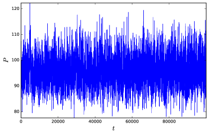
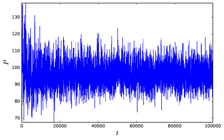
Figure 1: Stock time series for the initial (top to bottom, left to right) identical, uniform, normal, and Pareto wealth allocations in section 4. The stock price exhibits a mean-reverting behavior around the equilibrium price $\sim 96$.

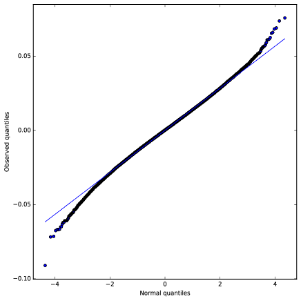
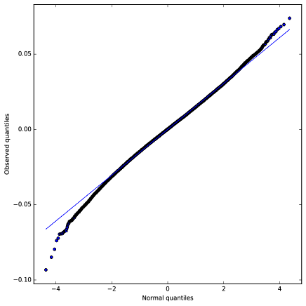
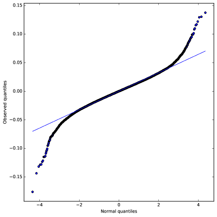
Figure 2: Quantile-quantile plots for the initial (top to bottom, left to right) identical ($R^{2}=0.999$, sd=$0.0142$), uniform ($R^{2}=0.999$, sd=$0.0152$), normal ($R^{2}=0.999$, sd=$0.0145$), and Pareto ($R^{2}=0.992$, sd=$0.0165$) wealth allocations in section 4.

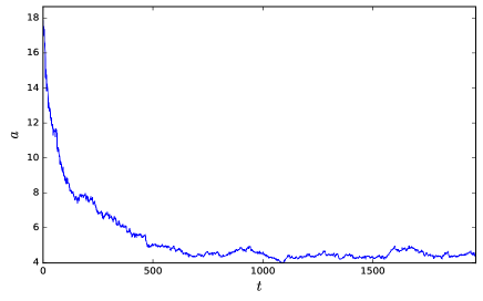
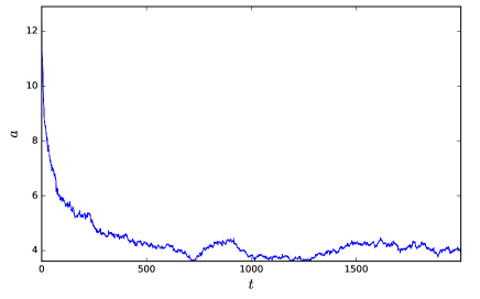
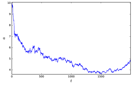
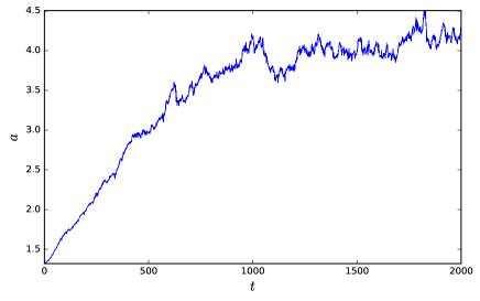
Figure 3: Evolution of the Pareto tail (richest 25% of the agents) fit power for the initial (top to bottom, left to right) identical (starting from step 30), uniform, normal, and Pareto wealth allocations in section 4. The measurements are taken every $50$ steps.

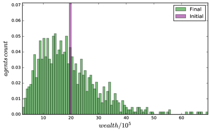
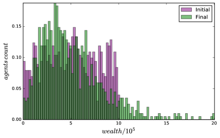
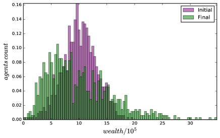
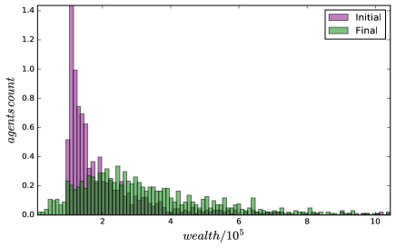
Figure 4: Initial and final wealth histogram for the starting (top to bottom, left to right) identical, uniform, normal, and Pareto wealth allocations in section 4.

In this section we are going to focus on the wealth dynamics in the participation sentiment-driven market environment set up in section 2. We will study how the market activity of $N=1000$ agents influences the wealth distribution dynamics over $T=10^{5}$ simulation steps. In each of the considered cases half of the initial portfolio value will be allocated in stock, and half in cash. We set the interest rate and the dividend yield identically to zero, $r=0$, $d=0$.

We will also assume that the breaking news volatility is identical to the calm volatility. Equivalently, we will assume that the volatility process (5) has infinite arrival time, $\lambda=\infty$. We set the calm volatility to be

$$\sigma_{c}={\cal N}(0.05,0.001)\,.$$ (13)

The inverse mean arrival time for the agents’s market participation sentiment process (6) will be set to

$$\rho^{-1}={\cal N}(0.1,0.01)\,.$$ (14)

In this section we will set the buy/sell dis-balance sentiment (2) to be identically zero, $\psi=0$. Then from (1) it follows that the equilibrium stock price around which the stock time series is expected to exhibit a mean-reverting behavior is equal to $M/S$, where $M$ is the total amount of cash and $S$ is the total number of shares outstanding. Since $r=0$ and $d=0$ the total amount of cash $M$ is time-independent. The total number of shares outstanding $S$ is also a constant. Initially every agent receives half a portfolio in cash, and half in stock, and therefore we expect the stock price to exhibit a mean-reverting behavior around the equilibrium value $M/S=P_{0}$, equal to the initial stock price.

However, running the simulation we observe that the stock price exhibits mean-reverting behavior around the equilibrium value $\sim 96$, see fig. 1. This is an artifact of the limit price choice, allocating a higher probability to the price lower than the last stock price, as discussed below eq. (4).

Besides the stock price times series we also are interested in the stock returns distribution and the wealth dynamics. We study the stock returns distribution by plotting a quantile-quantile plot against the standard normal quantiles for the logarithmic stock returns, see fig. 2. We observe that the stock returns are well approximated by the log-normal distribution, with the QQ fitting line having a zero intercept (mean return), and the slope (standard deviation) around $\sigma_{r}=0.015$. We will see below that turning on the jump diffusion sentiment will introduce significant deviation of the stock log-returns from the normal distribution.

The most prominent feature of fig. 2 is that the stock returns are most deviating from the log-normal distribution for the case when the initial wealth of the agents is Pareto-distributed. This property of the (small-exponent) Pareto society will be confirmed in other simulations in the subsequent sections. It is consistent with the observation [19] that since the Pareto society is realistically expected to have a few very rich agents, when those agents will be chosen to trade they will submit a large-sized orders. Such an orders will skew the supply-demand intersection point, resulting in a large price change.

We notice that regardless of the considered choices of the initial wealth allocation, the wealth distribution quickly acquires a Pareto tail with the exponent $a$ undergoing dynamics demonstrated in fig. 3. Eventually in all of the considered cases the Pareto tail exponent approaches the value $a\simeq 4$. This means that the exponent will go down (thickening the wealthy tail) for the considered initial identical, uniform, and normal wealth distribution. For the initial $a=1.5$ Pareto distribution it will go up, thinning the wealthy tail. We plot the initial and final wealth allocation histograms in fig. 4.

5 Including the buy/sell sentiment in the jump volatility market

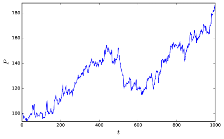
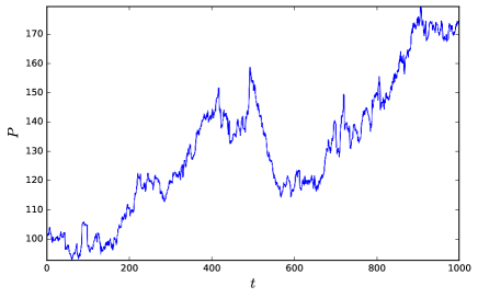
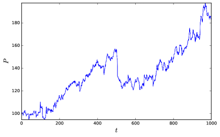
Figure 5: Stock time series for the initial (top to bottom, left to right) identical, uniform, normal, and Pareto wealth allocations in section 5.

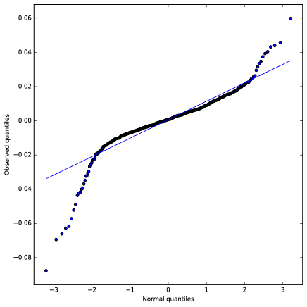
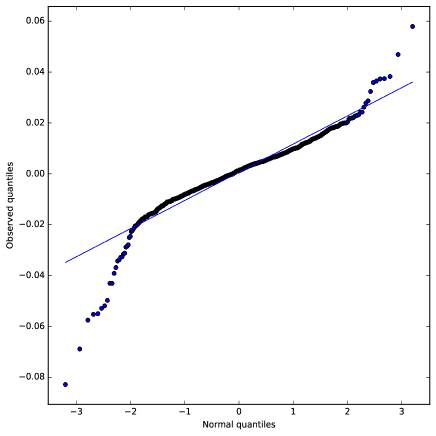
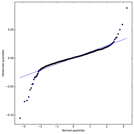
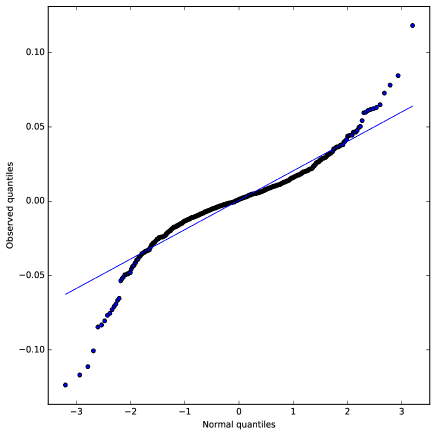
Figure 6: Quantile-quantile plots for the initial (top to bottom, left to right) identical ($R^{2}=0.93$, mean=$-0.0006$, sd=$0.01$), uniform ($R^{2}=0.95$, mean=$-0.0005$, sd=$0.01$), normal ($R^{2}=0.92$, mean=$-0.0006$, sd=$0.01$), and Pareto ($R^{2}=0.95$, mean=$-0.0006$, sd=$0.02$) wealth allocations in section 5.

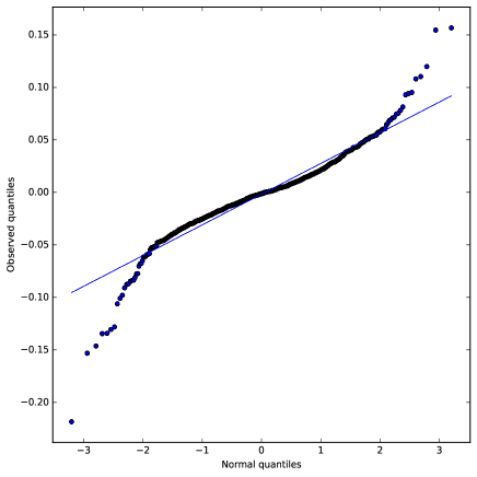
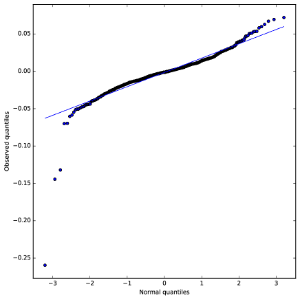
Figure 7: Quantile-quantile plots for: left TSLA ($R^{2}=0.96$, mean=$0.0018$, sd=$0.029$), right FB ($R^{2}=0.92$, mean=$0.0017$, sd=$0.019$), daily log returns over the period May 1, 2013-May 1, 2017.

In this section we are going to illustrate the influence of the buy/sell sentiment and the breaking news volatility sentiment on the stock price dynamics. We will consider evolution of the system of $N=1000$ agents over $T=1000$ steps. We will assume the per-step interest rate $r=10^{-3}$ and the vanishing dividend yield $d=0$.

We will also assume that the buy/sell sentiment is

$$\psi(t)=\left\{\begin{aligned} &{\cal N}(0,0.01),&&\text{if}\ t\in[0,T/2]\\ &{\cal N}(-0.3,0.01),&&\text{if}\ t\in[T/2,T]\end{aligned}\right.$$ (15)

This illustrates a simple attitude change in which at $t=T/2$ the stock receives a slight downgrade, which establishes the sell sentiment $e^{\psi}=p_{b}/p_{s}\simeq 0.74$. We know that according to (3) the change in the buy/sell sentiment $\psi$ will result in the change of the expected equilibrium stock price $P_{e}$. This effect is imposed on top of the overall stock price up-trend due to the cash inflow coming from the interest payments.

The calm volatility will be $\sigma_{c}={\cal N}(0.05,0.001)$, the breaking news volatility will be $\sigma_{b}={\cal N}(0.2,0.001)$. The breaking news inverse mean arrival time will be $\lambda^{-1}={\cal N}(0.08,10^{-4})$. The agents’s trading inverse mean arrival time will be $\rho^{-1}={\cal N}(0.3,0.01)$.

In fig. 5 we plot the simulated stock price time series. As expected, after step $t=500$ the stock price quickly declines to about $e^{-0.3}\simeq 0.74$ of its preceding value, in accord with (1). Notice that since all of the market participants experience the same sell over buy sentiment, the stock decline is rather steep. Also notice that in agreement with fig. 2 the Pareto society is the most volatile, due to the large orders submitted by exceptionally rich agents of the Pareto society [19].

In fig. 6 we plot the normal quantile-quantile plot of the stock log returns. As a frame of reference we provide the normal quantile-quantile plot for the TSLA and FB stocks daily returns over the period May 1, 2013-May 1, 2017, see fig. 7.

6 Subgroups of agents with different sentiments

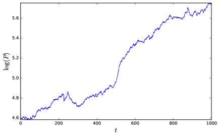
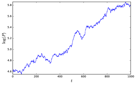
Figure 8: Time series of the logarithm of stock price for the initial (top to bottom, left to right) identical, uniform, normal, and Pareto wealth allocations in section 6.

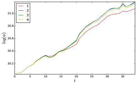
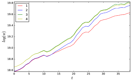
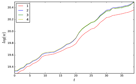
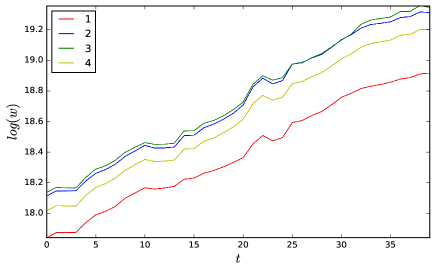
Figure 9: Logarithms of total wealth of each of the four groups of agents for the initial (top to bottom, left to right) identical, uniform, normal, and Pareto wealth allocations in section 6. The measurements are taken every 25 time steps. The groups 1, 2, 3, 4, defined in section 6 by their different buy/sell sentiments $\psi$, are color-labeled.

In section 5 we saw how switching on a sell sentiment experienced by all of the market participants results in a steep decline of the stock price, readjusting it according to eq. (3). It is natural to expect that if we activate the sell sentiment among only a subgroup of the market participants the stock decline will be more gradual.

In this section we consider the system of $N=1000$ agents trading over $T=1000$ steps. We will fix the interest rate to be $r=5\times 10^{-4}$. The dividend yield will be a non-trivial process

$$d=\left\{\begin{aligned} &{\cal N}(10^{-3},2\times 10^{-4}),&&\text{if}\ t\in[0,3T/4]\\ &0,&&\text{if}\ t\in[3T/4,T]\end{aligned}\right.$$ (16)

We will assume that the calm and breaking news volatilities are $\sigma_{c}={\cal N}(0.05,0.001)$, $\sigma_{b}={\cal N}(0.2,0.001)$, where the breaking news is the Poisson process arriving with the mean inverse time $\lambda^{-1}={\cal N}(0.005,0.0001)$. The agents will participate according to the Poisson process with the mean inverse arrival time $\rho^{-1}={\cal N}(0.6,0.01)$.

We will divide the agents into four groups with $250$ agents in each group. The groups 1, 2, 3, 4 will be fed the buy/sell sentiment process

$$\psi_{1} =\left\{\begin{aligned} &{\cal N}(0,0.1),&&\text{if}\ t\in[0,T/4]\\ &{\cal N}(-1,0.1),&&\text{if}\ t\in[T/4,T/2]\\ &{\cal N}(0,0.1),&&\text{if}\ t\in[T/2,3T/4]\\ &{\cal N}(-1,0.1),&&\text{if}\ t\in[3T/4,T]\end{aligned}\right.$$ (17)

$$\psi_{2} =\left\{\begin{aligned} &{\cal N}(0,0.1),&&\text{if}\ t\in[0,T/2]\\ &{\cal N}(0.1,0.1),&&\text{if}\ t\in[T/2,3T/4]\\ &{\cal N}(0,0.1),&&\text{if}\ t\in[3T/4,T]\end{aligned}\right.$$ (18)

$$\psi_{3} =\left\{\begin{aligned} &{\cal N}(0,0.1),&&\text{if}\ t\in[0,3T/4]\\ &{\cal N}(1,0.1),&&\text{if}\ t\in[3T/4,T]\\ \end{aligned}\right.$$ (19)

$$\psi_{4} ={\cal N}(0,0.1),\quad\text{if}\ t\in[0,T]\,.$$ (20)

The resulting stock evolution is plotted in fig. 8. We chose to plot the logarithm of stock price, to visualize better the price change on top of the exponential inflation. We can see a mild short-term decline starting at $t=T/4$ brought by the strong selling preference of the group 1 during the period $[T/4,T/2]$. The stock price also has a positive cusp at $t=T/2$, when the agents of group 1 become buy/sell neutral again, and the agents of group 2 develop a slight preference for buy over sell. At $t=3T/4$ group 1 acquires a strong sell preference, and group 3 acquires a strong buy preference, offsetting each other. The stock price still has a slight negative cusp at $t=3T/4$, due to vanishing dividend during the period $[3T/4,T]$, thereby reducing the cash inflow into the system, and consequently resulting in a lower slope of the stock inflation uptrend.

In fig. 9 we plot time dependence of the logarithm of the collective wealth of each of the four groups of agents, recording the wealth every 25 steps. The base reference is provided by the group 4 (yellow line) whose agents remained buy/sell neutral throughout the whole simulation. Before $t=T/4$ all the groups behave in a similar way: everyone is following a neutral buy/sell sentiment during that period.

At $t=T/4$ the group 1 (red line) starts preferring selling over buying, therefore driving the stock price down. The agents of group 1 are the least to suffer from the immediate stock decline, due to their relative pulling out of the stock market. The groups 2, 3, 4 are buy/sell neutral during that period, and their wealth evolves in a synchronous manner (as is best seen on the plot corresponding to the identical initial wealth allocation). However even before $t=T/2$ the negative gap develops between the wealth of the group 1 and the wealth of the groups 2, 3, 4. This is due to the fact that the groups 2, 3, 4, possessing more shares of stock than the group 1, have accumulated more of the dividend returns on the stocks.

At $t=T/2$ the group 1 becomes buy/sell neutral again, and starts acquiring more shares of stock. This, and the slight buy preference of the group 2 (blue line) during the time $[T/2,3T/4]$, results in a positive wealth cusp at $t=T/2$. The group 2 being the most invested, is expected to benefit the most from the stock price uptrend.

At $t=3T/4$ the group 1 starts actively pulling out of the stock market again and the group 3 (green line) starts actively buying into stocks. The stock does not issue dividends during the time interval $[3T/4,T]$. Notice that the activity of the group 3 offsets the activity of group 1. (We have confirmed this by running a similar simulation with identically vanishing $r$ and $d$, where it is clear to see if price trend develops, transitioning to a new equilibrium value.) Notice that since the stock does not pay dividend during the period $[3T/4,T]$, the money inflow into the system decreases, and as a result the stock price uptrend is only fueled by the cash interest payments received by the agents. Therefore the stock price, as well as the agents’s portfolios, have a smaller slope during that period, and a negative cusp at $t=3T/4$.

7 Discussion

In this paper we proposed and studied a simulated stock market environment with the sentiment drivers determining trading actions of participating agents. We have considered sentiments affecting the trading intensity, buy/sell preference, and stock price volatility. We have omitted entirely any strategy assignment to the agents. In our models the stock price behavior, observed during the simulation, does not influence the trading decisions made by the agents. This is in contrast with most of the literature dedicated to the artificial stock markets.

Our paper is to be applied to the study of stock market dynamics after the question of the market participants’s trading behavior has already been answered. We assume that the answer to that question boils down to specifying the sentiment processes followed by a large groups of the market participants. That is, our study of the stock dynamics is done in the framework where the market state is in one to one correspondence with the set of sentiment driving processes. Once existence of those sentiment processes is confirmed and their parameters are established, our paper can be used to determine the resulting stock price dynamics. The assumption that the agents will follow the sentiment after observing the stock price behavior emergent in the course of simulation is rather strong, and is used as a postulate for our sentiment-driven market framework.

We have studied several simulations in our proposed sentiment-driven market environment. We have noticed that, as expected, incorporation of a non-trivial volatility sentiment process results in a deviation of a large stock returns from the log-normal distribution. This is consistent with the actual observations of the statistical properties of stock price returns, and is typically sought to be reproduced in the stock market simulations. We have also demonstrated how a non-trivial buy/sell sentiment process creates a predictable price trends, and allows to manipulate the price dynamics away from a simple mean-reverting behavior. In particular we have studied the situation in which different subgroups of agents are influenced by different sentiments while trading with each other freely.

We have considered four possible kinds of initial wealth allocation: identical, uniform, normal, and Pareto, and studied the subsequent wealth dynamics of all and subgroups of the agents over the course of simulation. It is interesting that regardless of the considered initial wealth allocation, and consistent with the literature on this subject, the wealth distribution of the agents quickly acquires a power-law Pareto tail. We have studied how the Pareto exponent evolves in time.

A possible application of our model would be to use it as an ingredient of a trading strategy, built on the assumption that one can derive the properties of the stock market behavior, such as price trends/volatility and trade volume, by knowing what sentiment processes that behavior can be reduced to. Then observing the stock price time dependence we can use Bayesian inference to obtain the posterior likelihoods of the sentiment processes. This will allows us to have some idea of where so derived sentiments will lead the stock price.

8 Appendix: The stock exchange structure

In this appendix we describe design of our stock exchange. We have implemented all of our calculations in Python. The stock exchange is an interaction mediator for the agents. Each agent is characterized by a portfolio: the number of shares of stock, and the quantity of cash. Information about portfolios of agents is kept in the client book, which we describe in subsection 8.1. All of the market activity of agents is done through the intermediary of the stock exchange. At each time step the stock exchange begins by accepting orders from the agents. It records orders into the sorted tables of the order book, which we describe in subsection 8.2. Then it switches on the matching engine which tries to find a new equilibrium price by balancing the supply and demand for the shares of stock. If the equilibrium is reached, the matching engine fills all of the possible orders, as described in subsection 8.3. It then interfaces with the client book, and updates portfolios of the agents accordingly to the filled orders.

8.1 The client book

The purpose of the client book is to maintain the portfolio records of all of the agents, with each agent being assigned a unique client ID number. We implement the client book as a class which has an easy interface, allowing to add new clients, endow clients with the shares of stock and units of cash, modify client records, and delete clients. In our system each client will be allowed to maintain only one open order at a time. As described in the next subsection each order is identified by a unique order ID number. The client book maintains a table matching the order ID to the ID of the client who issued that order.

8.2 The order book

All of the orders from the agents go directly to the order book. The orders are characterized by the order ID number, the side (buy or sell), the limit price, and the size. We implement the order book as a class, which maintains separate dictionaries of buy and sell orders, matching the sorted prices to the sizes and identification numbers of the orders. The order book provides an easy interface allowing to add, modify, or cancel an order. If the stock exchange fills only a part of the order (as it frequently occurs for the orders at the price level equal to the exact intersection price of the supply and demand curves, see the next subsection) it will modify the corresponding order to the smaller size accordingly.

8.3 The matching engine

The center of the stock exchange is the matching engine. In our implementation the matching engine is a class which inherits from the client book and the order book classes, allowing it to interface directly with the client records and the order records. The matching engine has two main functionalities. The first is to match the orders of the order book, and determine the equilibrium price for the supply and demand. The second is to fill the orders, in accord with the matched price, and update the client book correspondingly.

The matching of orders in the order book is done by constructing the supply and demand curves on the price and volume plane and looking for intersection. The supply at price $P$ is given by all the sell orders at price $P$ and lower, and is therefore a non-decreasing function of price. The demand at price $P$ is given by all the buy orders at price $P$ and higher, and is therefore a non-increasing function of price. Both curves are discrete, and therefore resovling their intersection requires a careful consideration.

First of all, it might be that the intersection is never achieved. If the highest buy order price $P_{1}$ is strictly lower than the lowest sell order price $P_{2}$, then no orders can be filled. This is illustrated by the following figure.

We are plotting the supply curve (made up by the sell orders) using the punctured line, and the demand curve (made up by the buy orders) using the solid line. The horizontal axis is the price, the vertical axis is the volume of the orders, the base line represents zero volume. The supply curve (punctured line) starts at zero volume at zero price (no one wants to sell at zero price) and jumps up by $V_{s}$ each time we cross a price point $P_{s}$ of some sell order of the size $V_{s}$. The supply order saturates to the total volume of all the sell orders at the highest submitted sell order price, where everyone would be willing to sell. The demand curve (solid line) starts at the total demand volume (of all the buy orders combined) at zero price (everyone wants to buy at zero price). As the price goes up, each time we cross a price point $P_{b}$ of some buy order of the size $V_{b}$, the demand curve drops by $V_{b}$. After the highest submitted buy price price the demand is zero: no one wants to buy at the higher price.

If the intersection occurs, it can be of three possible types. The type of intersection determines the intersection price and volume, and resolves how the orders at the intersection price are filled. We categorize the intersection types according to what curve (supply or/and demand) is vertical at the intersection point.

• Buy cross. The demand curve is vertical at the intersection point.

  In this case all the sell orders at prices lower than $P_{*}$ can be filled, and the resulting volume $V_{*}$ is defined by the cumulative sell volume at $P_{*}$. We start filling the buy orders at the highest submitted buy price. We can first fill all those orders for the prices strictly higher than $P_{*}$. After this is achieved we will have $\Delta$ less buy orders filled than the sell orders. The $\Delta$ is in general a part of all the buy orders submitted at the price $P_{*}$. We fill them in the order of arrival (as determined by the order ID’s), and keep the rest of the orders in the order book.

• Sell cross. The supply curve is vertical at the intersection point. Symmetric to the buy cross w.r.t. the buy/sell exchange.

  In this case all the buy orders at prices higher than $P_{*}$ can be filled, and the resulting volume $V_{*}$ is defined by the cumulative buy volume at $P_{*}$. We start filling the sell orders at the lowest submitted sell price. We can first fill all those orders for the prices strictly lower than $P_{*}$. After this is achieved we will have $\Delta$ less sell orders filled than the buy orders. The $\Delta$ is in general a part of all the sell orders submitted at the price $P_{*}$. We fill them in the order of arrival, and keep the rest of the orders in the order book.

• Mixed cross. Both the supply and the demand curves are vertical at the intersection point. That is, there are buy and sell orders submitted at the price $P_{*}$. Depending on the buy and sell volumes at price $P_{*}$ there are two cases. In the first case we can fill all the sell orders and the fraction $\Delta$ of the buy orders.

  In the second case we can fill all the buy orders and the fraction $\Delta$ of the sell orders.

  The exact match is a particular case of the mixed cross with $\Delta=0$.

After the possible orders are filled, we can either keep the remaining orders in the order book pending, or clear up the order book.

References

References

- [1] R. G. Palmer, W. B. Arthur, J. H. Holland, B. LeBaron, and P. Tayler, Artificial economic life: a simple model of a stock market, Physica D, 75, 264, 1994.
- [2] W. B. Arthur, J. H. Holland, B. LeBaron, R. Palmer, and P. Tayler, Asset Pricing Under Endogenous Expectations in an Artificial Stock Market, 1996.
- [3] R. G. Palmer, W. B. Arthur, J. H. Holland, and B. LeBaron, An artificial stock market, Artificial life and robotics, 3, 1, 27, 1999.
- [4] B. LeBaron, W. B. Arthur, and R. Palmer, Time series properties of an artificial stock market, Journal of Economic Dynamics and Control, 23, 9, 1487, 1999.
- [5] M. Raberto, S. Cincotti, S. M. Focardi, and M. Marchesi, Agent-based simulation of a financial market, Physica A, 299, 1, 319, 2001.
- [6] E. Bonabeau, Agent-based modeling: methods and techniques for simulating human systems, Proceedings of the NAS of the USA, 99, 10, 3, 2002.
- [7] L. Ponta, M. Raberto, and S. Cincotti, A multi-assets artificial stock market with zero-intelligence traders, Europhysics Letters, 93, 2, 2011.
- [8] M. A. Bertella, F. R. Pires, L. Feng , H. E. Stanley, Confidence and the stock market: an agent-based approach, PLoS ONE, 9(1): e83488, 2014.
- [9] E. Samanidou, E. Zschischang, D. Stauffer, and T. Lux, Agent-based models of financial markets, Reports on Progress in Physics, 70, 3, 2007.
- [10] B. Mandelbrot, The variation of certain speculative prices, Fractals and scaling in finance, 371, 1997.
- [11] S. Pastore, L. Ponta, and S. Cincotti, Heterogeneous information-based artificial stock market, New Journal of Physics, 12, 2010.
- [12] R. Engle, J. Russel, Forecasting the frequency of changes in quoted foreign exchange prices with the autoregressive conditional duration model, Journal of Empirical Finance, 4, 187, 1997.
- [13] R. Engle, J. Russel, Autoregressive conditional duration: A new model for irregularly spaced transaction data, Econometrica, 66, 5, 1127, 1998.
- [14] L. Ponta, E. Scalas, M. Raberto, and S. Cincotti, Statistical analysis and agent-based microstructure modeling of high frequency financial trading, IEEE Journal of Selected Topics in Signal Processing, 6, 4, 2011.
- [15] J. C. Cox, The valuation of options for alternative stochastic processes, Journal of Financial Economics, 3, 1, 145, 1976.
- [16] R. C. Merton, Option pricing when underlying stock returns are discontinuous, Journal of Financial Economics, 3, 1, 125, 1976.
- [17] J-P. Bouchaud, M. Mezard, Wealth condensation in a simple model of economy, Physica A, 282, 3, 536, 2000.
- [18] Z. Huang, S. Solomon, Power, Levy, exponential and Gaussian-like regimes in autocatalytic financial systems, European Physical Journal, B, 20, 601, 2001.
- [19] M. Raberto, S. Cincotti, S. Focardi, and M. Marchesi, Traders long-run wealth in an artificial financial market, Computational Economics, 22, 2, 255, 2003.
- [20] M. Levy and S. Solomon, New evidence for the power-law distribution of wealth, Physica A, 242, 1, 90, 1997.
- [21] M. Milakovic, Towards a Statistical Equilibrium Theory of Wealth Distribution, PhD thesis, 2003.
- [22] C. Castaldi and M. Milakovic, Turnover activity in wealth portfolios, Journal of Economic Behavior and Optimization, 63, 3, 537, 2007.
- [23] D. K. Foley, A statistical equilibrium theory of markets, Journal of Economic Theory, 62, 321, 1994.
- [24] E. T. Jaynes, Information theory and statistical mechanics, Physical Review D, 106, 620, 1957.
- [25] T. Lux, Applications of Statistical Physics in Finance and Economics, Kiel Working Paper, 1425, 2008.
- [26] H. Markowitz, Portfolio selection, The Journal of Finance, 7, 1, 1952.