A Numerical Relativity Waveform Surrogate Model for Generically Precessing Binary Black Hole Mergers

Abstract

A generic, non-eccentric binary black hole (BBH) system emits gravitational waves (GWs) that are completely described by 7 intrinsic parameters: the black hole spin vectors and the ratio of their masses. Simulating a BBH coalescence by solving Einstein’s equations numerically is computationally expensive, requiring days to months of computing resources for a single set of parameter values. Since theoretical predictions of the GWs are often needed for many different source parameters, a fast and accurate model is essential. We present the first surrogate model for GWs from the coalescence of BBHs including all $7$ dimensions of the intrinsic non-eccentric parameter space. The surrogate model, which we call NRSur7dq2, is built from the results of $744$ numerical relativity simulations. NRSur7dq2 covers spin magnitudes up to $0.8$ and mass ratios up to $2$, includes all $\ell\leq 4$ modes, begins about $20$ orbits before merger, and can be evaluated in $\sim~{}50\,\mathrm{ms}$. We find the largest NRSur7dq2 errors to be comparable to the largest errors in the numerical relativity simulations, and more than an order of magnitude smaller than the errors of other waveform models. Our model, and more broadly the methods developed here, will enable studies that were not previously possible when using highly accurate waveforms, such as parameter inference and tests of general relativity with GW observations.

I Introduction

With LIGO’s two confident detections of gravitational waves (GWs) from binary black hole (BBH) systems Abbott et al. (2016a, b), we have entered the exciting new era of GW astronomy. The source black hole (BH) masses and spins can be determined by comparing the signal to waveforms predicted by general relativity (GR)  Abbott et al. (2016c, d), and new strong-field tests of GR can be performed Abbott et al. (2016e). These measurements and tests require GW models that are both accurate and fast to evaluate. The total mass of the system $M$ can be scaled out of the problem, leaving a $7$-dimensional non-eccentric intrinsic parameter space over which the waveform must be modeled, consisting of the mass ratio and two BH spin vectors.

Numerical relativity (NR) simulations of BBH mergers Pretorius (2005); Zlochower et al. (2005); SpE (a); ein ; Husa et al. (2008); Brügmann et al. (2008); Herrmann et al. (2007) solve the full Einstein equations and produce the most accurate waveforms. These simulations are computationally expensive, requiring weeks to months on dozens of CPU cores for a waveform beginning $\sim 20$ orbits before the merger. Analytic and semi-analytic waveform models Damour et al. (2008); Damour and Nagar (2009); Taracchini et al. (2014); Pürrer (2016); Pan et al. (2013); Bohé et al. (2017); Hannam et al. (2014); Khan et al. (2016); Husa et al. (2016) are quick to evaluate, but they make approximations that can introduce differences with respect to the true waveform predicted by GR. These differences could lead to parameter biases or inaccurate tests of GR for some high signal-to-noise ratio detections that could be made in the near future Lindblom et al. (2008); Abbott et al. (2016f).

A surrogate waveform model Blackman et al. (2017, 2015); Field et al. (2014); Pürrer (2014, 2016) is a model that takes a set of precomputed waveforms that were generated by some other model (e.g., NR or a semianalytic model), and interpolates in parameter space between these waveforms to quickly produce a waveform for any desired parameter values. A surrogate waveform can be evaluated much more quickly than the underlying model, and can be made as accurate as the underlying model given a sufficiently large set of precomputed waveforms that cover the parameter space. Previous surrogate models based on NR waveforms were built for non-spinning BBH systems Blackman et al. (2015) and for a $4$-dimensional ($4d$) parameter subspace containing precession Blackman et al. (2017). Here, we present the first NR surrogate model including all $7$ dimensions of the parameter space. The model, which we call NRSur7dq2, produces waveforms nearly as accurate as those from NR simulations, but can be evaluated in $\sim~{}50\,\mathrm{ms}$ on a single CPU core for a speedup of more than $8$ orders of magnitude compared to NR. Our method enables performing high accuracy GW data analysis, including parameter inference for astrophysics and tests of GR.

II Numerical Relativity Data

The NR simulations used to build the surrogate model are performed using the Spectral Einstein Code (SpEC) SpE (a); Pfeiffer et al. (2003); Lovelace et al. (2008); Lindblom et al. (2006); Szilágyi et al. (2009); M. A. Scheel, M. Boyle, T. Chu, L. E. Kidder, K. D. Matthews and H. P. Pfeiffer (2009); Szilágyi (2014). The simulations begin at a coordinate time $\tau=0$, where we specify the BH mass ratio $q=m_{1}/m_{2}\geq 1$ and initial dimensionless spin vectors

$$\vec{\chi}_{i}(\tau=0)=\vec{S}_{i}(\tau=0)/m_{i}^{2}\,,\,\,i\in\{1,2\}\,.$$ (1)

The system is evolved through merger and ringdown, and the GWs are extracted at multiple finite radii from the source. These are extrapolated to future null infinity Boyle and Mroué (2009) using quadratic polynomials in $1/r$, where $r$ is a radial coordinate. The effects of any drifts in the center of mass that are linear in time are removed from the waveform Boyle (2016, 2013); Boyle et al. (2014); scr . The waveforms at future null infinity use a time coordinate $\tilde{\tau}$, which is different from the simulation time $\tau$, and begins approximately at $\tilde{\tau}=0$. The spins $\vec{\chi}_{i}(\tau)$ are also measured at each simulation time. To compare spin and waveform features, we identify $\tau$ with $\tilde{\tau}$. While this identification is not gauge-independent, the spin directions are already gauge-dependent. We note that the spin and orbital angular momentum vectors in the damped harmonic gauge used by SpEC agree quite well with the corresponding vectors in post-Newtonian (PN) theory Ossokine et al. (2015).

Once we have the spins $\vec{\chi}_{i}(\tau)$ and spin-weighted spherical harmonic modes of the waveform $h^{\ell,m}(\tau)$, we perform the same alignment discussed in Sec. III.D of Ref. Blackman et al. (2017). Briefly, for each simulation, we first determine the time $\tau_{\mathrm{peak}}$ which maximizes the total amplitude of the waveform

$$A_{\mathrm{tot}}(\tau)=\sqrt{\sum_{\ell,m}|h^{\ell,m}(\tau)|^{2}}\,.$$ (2)

We determine $\tau_{\mathrm{peak}}$ by fitting a quadratic function to $5$ adjacent samples of $A_{\mathrm{tot}}(\tau)$, consisting of the largest sample and two neighbors on either side. We choose a new time coordinate

$$t=\tau-\tau_{\mathrm{peak}}\,,$$ (3)

which maximizes $A_{\mathrm{tot}}$ at $t=0$. We then rotate the waveform modes such that at our reference time of $t=t_{0}=-4500M$, $\hat{z}$ is the principal eigenvector of the angular momentum operator Boyle et al. (2011) and the phases of $h^{2,2}(t_{0})$ and $h^{2,-2}(t_{0})$ are equal. We sample the waveform and spins in steps of $\delta t=0.1M$, from $t_{0}$ to $t_{f}=100M$, by interpolating the real and imaginary parts of each waveform mode, as well as the spin components, using cubic splines. The initial separations and velocities of the BBH systems were chosen such that, after aligning the peak amplitude to $t=0$ as above, the waveforms begin at $t\approx-5000M$. Choosing $t_{0}=-4500M$ discards the first $\sim 500M$ which is contaminated by junk radiation Aylott et al. (2009).

We first include all $276$ NR simulations used in the NRSur4d2s surrogate model and the $9$ additional simulations used in Sec. IV.D and Table V of Ref. Blackman et al. (2017). We perform $459$ additional NR simulations. The first $361$ of these are chosen based on sparse grids Smolyak (1963); Bungartz and Griebel (2004) and include combinations of extremal parameter values (such as $q\in\{1,2\}$) and intermediate values as detailed in Appendix A. The parameters for the remaining $98$ simulations are chosen as follows. We randomly sample $1000$ points in parameter space uniformly in mass ratio, spin magnitude, and spin direction on the sphere. We compute the distance between points $a$ and $b$ using

$$ds^{2}=\left(0.3\left(q_{a}-q_{b}\right)\right)^{2}+\sum_{i\in\{1,2\}}\left\|\vec{\chi}_{ia}-\vec{\chi}_{ib}\right\|^{2}\,.$$ (4)

The coefficients multiplying each term in this expression have been chosen somewhat arbitrarily, although our expectation is that any choice of order unity should provide a reasonable criteria for point selection. For each sampled parameter, we compute the minimum distance to all previously chosen parameters. We then choose the sampled parameter maximizing this minimum distance. We then resample the $1000$ parameters for the next of the $98$ iterations. This results in a total of $744$ NR simulations. For simulations with equal masses and unequal spins, we use the results twice by reversing the labeling of the BHs and rotating the waveform accordingly. There are $142$ such simulations, leading to $886$ NR waveforms.

III Waveform Decomposition

The goal of a surrogate model is to take a precomputed set of waveform modes $\{h_{i}^{\ell,m}(t)\}$ at a fixed set of points in parameter space $\{\vec{\lambda}_{i}\}$, and to produce waveform modes $\{h^{\ell,m}(t)\}$ at new desired parameter values. Because $h^{\ell,m}(t)$ is highly oscillatory and changes in a complicated way as one varies the masses and spins, it is not feasible to directly interpolate $\{h_{i}^{\ell,m}(t)\}$ in parameter space with only $886^{1/7}\approx 2.64$ available points per dimension. Instead, we decompose each waveform $h(t)$ into many waveform data pieces. Each waveform data piece is a simpler function that varies slowly over parameters. Once we have interpolated each waveform data piece to a desired point in parameter space, we recombine them to form $h(t)$. Our decomposition is similar to but improves upon the one used in Ref. Blackman et al. (2017).

We first determine the unit quaternions $\hat{q}(t)$ that define the coprecessing frame Schmidt et al. (2011); O’Shaughnessy et al. (2011); Boyle et al. (2011), and we determine the waveform modes $\{h_{C}^{\ell,m}(t)\}$ in this frame. This is done using the transformation $T_{C}$ given by Eq. 25 of Ref. Blackman et al. (2017). The orbital phase

$$\varphi(t)=\frac{1}{4}\left(\arg\left[h_{C}^{2,-2}(t)\right]-\arg\left[h_{C}^{2,2}(t)\right]\right)\,,$$ (5)

is computed from the coprecessing waveform modes. This is expected to be superior to computing the orbital phase from the BH trajectories because unlike the coordinate-dependent trajectories, the waveform can be made gauge invariant up to Bondi-Metzner-Sachs transformations Boyle (2016).

We filter the spins $\vec{\chi}_{i}$ in the inertial frame using the same Gaussian filter that was used to filter $\hat{q}(t)$ in Ref. Blackman et al. (2017), and note that here we do not filter $\hat{q}(t)$. The filtered spins are given by

$$\vec{\chi}_{i}^{\mathrm{filt}}(t)=\frac{\int_{\varphi_{-}}^{\varphi_{+}}\vec{\chi}_{i}(t^{\prime}(\varphi))G(\varphi)d\varphi}{\int_{\varphi_{-}}^{\varphi_{+}}G(\varphi)d\varphi}\,,$$ (6)

where $t^{\prime}(\varphi)$ is the inverse function of Eq. 5, and $\varphi_{\pm}$ and $G(\varphi)$ are given by Eqs. 39-43 of Ref. Blackman et al. (2017). Note that $\varphi_{\pm}$ and $G(\varphi)$ implicitly depend on $t$. The spins are then transformed to the coprecessing frame using

$$\vec{\chi}_{i}^{\mathrm{copr}}(t)=\hat{q}^{-1}(t)\vec{\chi}_{i}^{\mathrm{filt}}(t)\hat{q}(t)\,.$$ (7)

Note that quaternion multiplication is used here, and vectors are treated as quaternions with zero scalar component. We find that filtering the spins leads to a more accurate surrogate model by suppressing the orbital timescale oscillations in the spin components Ossokine et al. (2015) and therefore making the spin time derivatives easier to model.

We then transform the spins and waveform modes to a coorbital frame, in which the BHs are nearly on the $x$ axis. The coorbital frame is just the coprecessing frame rotated by $\varphi(t)$ about the $z$ axis. Specifically, we have

$$\hat{q}_{\mathrm{r}}(t) =\cos\left(\frac{\varphi(t)}{2}\right)+\hat{z}\sin\left(\frac{\varphi(t)}{2}\right)\,,$$ (8)

$$\vec{\chi}_{i}^{\mathrm{coorb}}(t) =\hat{q}^{-1}_{\mathrm{r}}(t)\vec{\chi}_{i}^{\mathrm{copr}}(t)\hat{q}_{\mathrm{r}}(t)\,,$$ (9)

$$h^{\ell,m}_{\mathrm{coorb}}(t) =h^{\ell,m}_{C}(t)e^{im\varphi(t)}\,,$$ (10)

where $\hat{q}_{\mathrm{r}}(t)$ is a unit quaternion representing a rotation about the $\hat{z}$ axis by $\varphi$. Finally, using $4$th order finite differences, we compute the orbital frequency

$$\omega(t)=\frac{d}{dt}\varphi(t)$$ (11)

and the spin time derivatives in the coprecessing frame, which we then transform to the coorbital frame

$$\dot{\vec{\chi}}_{i}^{\mathrm{coorb}}(t)=\hat{q}^{-1}_{\mathrm{r}}(t)\dot{\vec{\chi}}_{i}^{\mathrm{copr}}(t)\hat{q}_{\mathrm{r}}(t)\,,$$ (12)

where a dot means $d/dt$. For the precession dynamics, we compute the angular velocity of the coprecessing frame

$$\frac{1}{2}\vec{\Omega}^{\mathrm{copr}}(t) =\lim_{dt\rightarrow 0}\frac{1}{dt}\left(\hat{q}^{-1}(t)\hat{q}(t+dt)-1\right)$$ (13)

$$=s(t)\dot{\vec{v}}(t)-\dot{s}(t)\vec{v}(t)-\vec{v}(t)\times\dot{\vec{v}}(t)\,,$$ (14)

where $s(t)$ and $\vec{v}(t)$ are the scalar and vector components of $\hat{q}(t)$. Fourth-order finite difference stencils are used to compute the time derivatives appearing in Eq. (14). We also transform $\vec{\Omega}^{\mathrm{copr}}(t)$ to the coorbital frame to obtain $\vec{\Omega}^{\mathrm{coorb}}(t)$ as in Eq. (12). The minimal rotation condition of the coprecessing frame ensures

$$\Omega_{z}^{\mathrm{coorb}}(t)=\Omega_{z}^{\mathrm{copr}}(t)=0$$ (15)

up to finite difference errors.

Given a waveform data piece $X(t)$ evaluated at a set of parameters, one would be tempted to parameterize $X(t)$ at any fixed time $t_{i}$ by the mass ratio and the initial spins, and then construct a fit to $X(t_{i})$ as a function of these parameters. However, we find much better fits if we instead parameterize $X(t_{i})$ by the spins at time $t_{i}$ and the mass ratio. While this is easy to do during the inspiral where we still have two BHs with individual spins, we seek a way to extend this parameterization through the merger and ringdown, where individual BH spins are no longer available. We extend, unphysically, the spin evolution through the merger and ringdown using the PN expressions

$$\frac{d}{dt}\vec{\chi}_{i}=\vec{\Omega}_{i}^{\mathrm{Spin}}\times\vec{\chi}_{i}\,,$$ (16)

where $\vec{\chi}_{i}$ is the spin in the inertial frame, and $\vec{\Omega}_{i}^{\mathrm{Spin}}$ is a PN expression given by Eq. A32 of Ref. Ossokine et al. (2015). $\vec{\Omega}_{i}^{\mathrm{Spin}}$ is a function of the orbital angular momentum vector $\hat{l}(t)$, a vector pointing from one BH to the other $\hat{n}(t)$, and the PN parameter $x(t)$. Evaluating $\vec{\Omega}_{i}^{\mathrm{Spin}}$ requires several quantities that are typically computed from BH trajectories in PN theory. Since the trajectories are also not available after the merger, we compute them from the waveform. We take $\hat{l}$ and $\hat{n}$ to be the $\hat{z}$ and $\hat{x}$ axes of the coorbital frame, and we take the PN parameter $x$ to be $\omega^{2/3}$, where $\omega$ is defined in Eq. (11) (see Eq. 230 of Ref. Blanchet (2014)). We choose $t_{\mathrm{PN}}=-100M$ and begin the PN integrations from the spins at $t_{\mathrm{PN}}$. The extended spins are somewhat robust to the choice of $t_{\mathrm{PN}}$ as seen in Fig. 1. We stress that these extended spins are not physically meaningful for $t>t_{\mathrm{PN}}$, but provide a convenient parameterization of the system that leads to accurate parametric fits.

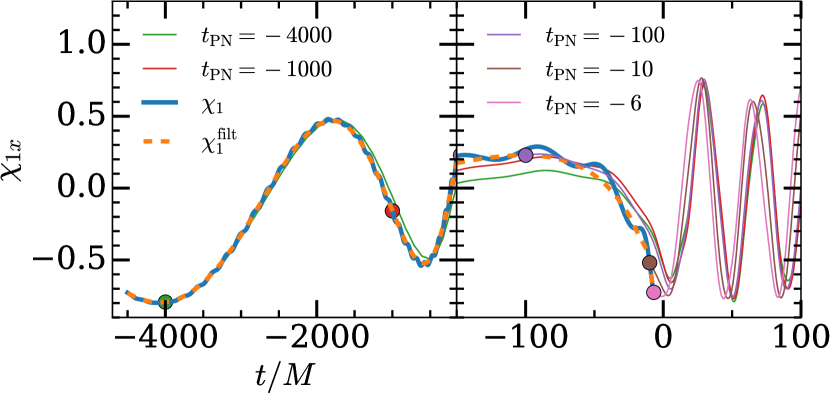
Figure 1: The $x$-component of a spin extended through merger and ringdown with PN expressions. These spins are not physically meaningful, but provide a parameterization of the system leading to accurate fits. The thick solid blue curve and dashed orange curve show the unfiltered and filtered spins from an NR simulation, and are not measured past $t=-6M$ due to the merger of the BHs. Each thin line is identical to the filtered NR curve before some time $t_{\mathrm{PN}}$ indicated with a dot, after which the spins are evolved using Eq. (16). The spins during the ringdown are affected somewhat by the choice of $t_{\mathrm{PN}}$, but the overall phasing is quite similar.

IV Building the Model

In this section, we describe the quantities that are computed from the waveform data pieces and stored when building the NRSur7dq2 surrogate model. The subsequent section will then describe how the NRSur7dq2 surrogate model uses these stored quantities to generate waveforms.

We first construct surrogate models for the waveform modes in the coorbital frame $h^{\ell,m}_{\mathrm{coorb}}(t)$. For $m=0$ modes, we directly model the real and imaginary components without any additional decompositions. For $m>0$, we compute

$$h^{\ell,m}_{\pm}=\frac{1}{2}\left(h^{\ell,m}_{\mathrm{coorb}}\pm h^{\ell,-m\,*}_{\mathrm{coorb}}\right)$$ (17)

and model the real and imaginary parts of $h^{\ell,m}_{\pm}$. Each of these modeled components is considered a waveform data piece. We proceed according to Sec. V of Ref. Blackman et al. (2017): For each waveform data piece, we construct a compact linear basis using singular value decomposition with a RMS tolerance of $3\times 10^{-4}.$ We then construct an empirical interpolant and determine one empirical node time $T_{j}$ for each basis vector. The times $T_{j}$ are chosen differently for each waveform data piece. Finally, for each $T_{j}$, we construct a parametric fit for the waveform data piece evaluated at $T_{j}$, which is described below. The fits are functions of the mass ratio and the coorbital spin components $\vec{\chi}^{\mathrm{coorb}}_{i}(t)$ evaluated at $T_{j}$. Note that the $x$ component of a vector in the coorbital frame is roughly the component in the direction of a vector pointing from one BH to the other, the $z$ component is along the axis of orbital angular momentum, and the $y$ component is the remaining orthogonal direction. In addition to the resulting fit data, the empirical interpolation matrix (see Eq. (B7) of Ref.Field et al. (2014)) for each of these waveform data pieces is stored in the NRSur7dq2 surrogate model.

These parametric fits use the forward-stepwise greedy fitting method described in Appendix A of Ref. Blackman et al. (2017). One benefit of this fitting method is that it automatically selects for higher order fits whenever the data is high-quality (e.g. in the inspiral), and lower order fits whenever the data is more noisy (e.g. during the ringdown). We choose the basis functions to be a tensor product of 1D monomials in the spin components and

$$x=\frac{q-1.5}{0.51}\,,$$ (18)

which is an affine mapping from $[0.99,2.01]$ to the standard interval $[-1,1]$. We consider up to cubic functions in $x$ and up to quadratic functions in the spin components. We perform $20$ trials using $50$ validation points each. The fit coefficients and the basis functions selected during the fitting procedure are stored in the NRSur7dq2 surrogate model.

We also construct parametric fits for $\omega(t)$, $\Omega_{\{x,y\}}^{\mathrm{coorb}}(t)$, and $\dot{\chi}_{j\{x,y,z\}}^{\mathrm{coorb}}(t)$ at selected time nodes $t_{i}$. These quantities describe the dynamics of the binary and the spins, so we call these $t_{i}$ the dynamics time nodes. We attempt to choose the time nodes $t_{i}$ to be approximately uniformly spaced in $\varphi(t)$ with $10$ nodes per orbit. Because $\varphi(t)$ is different for different simulations, and we choose the same time nodes for all simulations, in practice our choice of $238$ time nodes gives us between $8$ and $15$ nodes per orbit. We find that this is sufficient — including additional nodes per orbit does not improve the accuracy of the surrogate model. Our time nodes are labeled $t_{0}<t_{1}<\dots<t_{234}=100M$ plus three additional nodes $t_{\frac{1}{2}}$, $t_{\frac{3}{2}}$, and $t_{\frac{5}{2}}$, which are the midpoints of their adjacent integer time nodes. The reason for including the fractional time nodes is for Runge-Kutta time integration at the beginning of the time series, which will be made clear in the next section. In Appendix B, we describe in detail the algorithm for choosing $t_{i}$, but any choice that is roughly uniformly-spaced in $\varphi(t)$ and sufficiently dense should yield a surrogate with comparable accuracy.

V Evaluating the model

To evaluate the NRSur7dq2 surrogate model, we provide the mass ratio $q$ and initial spins $\vec{\chi}_{j}(t_{0})$ as inputs. The evaluation consists of three steps: we first integrate a coupled ODE system for the spins, the orbital phase, and the coprecessing frame, then we evaluate the coorbital waveform modes, and finally we transform the waveform back to the inertial frame. We describe each of these steps below.

We initialize the ODE system with

$$\varphi(t_{0})=0\,,\quad\hat{q}(t_{0})=1\,,\quad\vec{\chi}_{j}^{\mathrm{copr}}(t_{0})=\vec{\chi}_{j}(t_{0})\,.$$

To integrate this system forward in time using a numerical ODE solver (described below), we need to evaluate the time derivatives of $\varphi$, $\hat{q}$, and $\vec{\chi}_{j}^{\mathrm{copr}}$ at a time node $t_{i}$, given the values of those variables at $t_{i}$. To do this, we first determine $\vec{\chi}_{j}^{\mathrm{coorb}}(t_{i})$ by rotating the $x$ and $y$ components of $\vec{\chi}_{j}^{\mathrm{copr}}(t_{i})$ by an angle $\varphi(t_{i})$ as in Eq. (10). We then evaluate the fits for $\omega(t_{i})$, $\Omega^{\mathrm{coorb}}_{\{x,y\}}(t_{i})$, and $\dot{\chi}_{j\{x,y,z\}}^{\mathrm{coorb}}(t_{i})$ using the mass ratio $q$ and the current coorbital spins $\vec{\chi}_{j}^{\mathrm{coorb}}(t_{i})$. We set $\Omega^{\mathrm{coorb}}_{z}(t_{i})=0$, and obtain $\dot{\vec{\chi}}_{j}^{\mathrm{copr}}(t_{i})$ and $\vec{\Omega}^{\mathrm{copr}}(t_{i})$ by rotating the $x$ and $y$ components of the corresponding coorbital quantities by an angle of $-\varphi(t_{i})$. We evolve the coprecessing vectors instead of the coorbital vectors because the former evolve on the longer precession timescale, allowing us to take large timesteps. Finally, after computing

$$\left.\frac{d}{dt}\hat{q}(t)\right\rvert_{t_{i}}=\frac{1}{2}\hat{q}(t_{i})\vec{\Omega}^{\mathrm{copr}}(t_{i})\,,$$ (19)

we obtain the time derivatives of $\varphi$, $\hat{q}$, and $\vec{\chi}_{j}^{\mathrm{copr}}$ at $t=t_{i}$.

These time derivatives are then used to integrate $\varphi$, $\hat{q}$, and $\vec{\chi}_{j}^{\mathrm{copr}}$ using an ODE solver. We desire an ODE integration method that uses few evaluations of the time derivatives to keep the computational cost of evaluating the model low. We use a fourth-order Adams-Bashforth method Butcher (2003); Bashforth and Adams (1883) detailed in Appendix C, which determines the solutions at the next node based on the time derivatives at the current and three previous nodes. This allows us to reuse fit evaluations from the previous nodes, and requires only one additional evaluation of the fits per node compared to four evaluations for a fourth-order Runge-Kutta scheme. The Adams-Bashforth integration is initialized by performing the first integration steps with fourth-order Runge-Kutta. This is why we include the three additional time nodes $t_{\frac{1}{2}}$, $t_{\frac{3}{2}}$ and $t_{\frac{5}{2}}$; they enable evaluating the midpoint increments of the initial Runge-Kutta scheme. Once we have evaluated the solutions at the time nodes $t_{i}$, we use cubic spline interpolation to determine the solutions at all times.

Now that we have $\varphi$, $\hat{q}$, and $\vec{\chi}_{j}^{\mathrm{copr}}$ for all $t$, we then evaluate each coorbital waveform data piece. This is done by first evaluating the fits at the empirical nodes $T_{i}$ using the mass ratio $q$ and the coorbital spins at the empirical nodes $\vec{\chi}_{j}^{\mathrm{coorb}}(T_{i})$, and then evaluating the empirical interpolant to obtain the waveform data piece at all times. Finally, we transform the coorbital frame waveform modes back to the coprecessing frame using $\varphi(t)$ and then to the inertial frame using $\hat{q}(t)$. The NRSur7dq2 surrogate data and Python evaluation code can be found at SpE (b).

To reduce the computational cost of transforming the coprecessing waveform modes to the inertial frame using $\hat{q}(t)$, which takes $\sim~{}1\,\mathrm{s}$ using all $\ell\leq 4$ modes sampled with $\delta t=0.1M$, we reduce the number of time samples of the coorbital waveform data pieces by using non-uniform time steps. We choose $2000$ time samples that are roughly uniformly spaced in the orbital phase, using the same method used to choose the dynamics time nodes described in Appendix B. This is sufficiently many time samples to yield negligible errors when interpolating back to the dense uniformly-spaced time array using cubic splines on the real and imaginary parts of the waveform modes.

Integrating the ODE system takes $\sim~{}3\,\mathrm{ms}$, where the numerical computations are performed by a Python extension written in C. Interpolating the results of the ODE integration to the $2000$ time samples described above takes $\sim~{}2\,\mathrm{ms}$ using cubic splines. Evaluating the coorbital waveform surrogate takes $\sim~{}4\,\mathrm{ms}$, and transforming the modes to the inertial frame takes $\sim~{}16\,\mathrm{ms}$, for a total of $\sim~{}25\,\mathrm{ms}$. Variations in the evaluation time can increase this up to $\sim~{}30\,\mathrm{ms}$. Restricting to only $\ell=2$ modes can reduce this time to $\sim~{}10\,\mathrm{ms}$. If we wish to sample the surrogate waveform at the same time nodes as the original numerical relativity simulations, which is a uniformly-spaced time array with $\delta t=0.1M$, the modes are interpolated to these points using cubic splines. This requires $\sim~{}6\,\mathrm{ms}$ per mode, for a total time of $\sim~{}150\,\mathrm{ms}$ when all $\ell\leq 4$ modes are interpolated in this way. We note, however, that the original NR simulations are oversampled for typical GW data analysis purposes. For example, a sampling rate of $4096\,\mathrm{Hz}$ for a $M=60M_{\odot}$ binary has $\delta t\approx 0.83M$, leading to an evaluation time of $\sim~{}50\,\mathrm{ms}$. All timings were done on Intel Xeon E5-2680v3 cores running at 2.5GHz.

VI Surrogate Errors

We use two error measures to quantify the accuracy of the surrogate model. Given two sets of waveform modes $h_{1}$ and $h_{2}$, we first compute

$$\mathcal{E}[h_{1},h_{2}]=\frac{1}{2}\frac{\sum_{\ell,m}\int_{t_{0}}^{t_{f}}|h_{1}^{\ell,m}(t)-h_{2}^{\ell,m}(t)|^{2}dt}{\sum_{\ell,m}\int_{t_{0}}^{t_{f}}|h_{1}^{\ell,m}(t)|^{2}dt}\,,$$ (20)

which is introduced in Eq. (21) of Blackman et al. (2017). Since we have aligned all the NR waveforms at $t=t_{0}$ and the surrogate model reproduces this alignment, we do not perform any time or phase shifts when computing $\mathcal{E}$.

For these comparisons, we use modes $\ell\leq 5$; if a mode is not included in a particular waveform model, we assume this mode is zero for that model. Since the NRSur7dq2 model does not contain $\ell=5$ modes, this ensures that the errors discussed below include the effect of neglecting $\ell=5$ and higher modes.

Histograms of $\mathcal{E}$ for all $886$ NR waveforms are given in Fig. 2. For all curves in the figure, $h_{1}$ is the highest available resolution NR waveform. For the thick solid black curve, $h_{2}$ is the same NR waveform as $h_{1}$, except computed at a lower numerical resolution, so this curve represents an estimate of the numerical truncation error in the NR waveforms used to build the surrogate model. For the solid blue curve, $h_{2}$ is the NRSur7dq2 surrogate waveform evaluated with the same mass ratio and initial spins of $h_{1}$. Note that since the surrogate was trained using all NR waveforms, this is an in-sample error.

The remaining curves in Fig. 2 indicate the in-sample error contribution from each of the three main waveform data pieces in the surrogate waveform: the orbital phase $\varphi$ (dash-dotted green curve), the quaternions $\hat{q}$ representing the precession (dashed orange curve), and the waveform modes in a coorbital frame $h_{\mathrm{coorb}}$ (thin solid red curve). For these curves, $h_{2}$ is computed by using the surrogate evaluation for one waveform data piece and the NR evaluation of the other pieces. The orbital phase errors give rise to the largest surrogate errors, indicating that efforts to improve the surrogate model should be focused on improving the orbital phasing.

Figure 2: Error histograms for $\mathcal{E}$ defined in Eq. (20), normalized such that the area under each curve is $1$ when integrated over $\mathrm{log}_{10}(\mathcal{E})$. The largest surrogate errors are comparable to the largest NR resolution errors, which compare high and medium resolution NR simulations to estimate the error in the NR waveforms. The error in the orbital phase $\varphi$ is the dominant error contribution to the surrogate.

We then compute mismatches Babak et al. (2017)

$$1-\frac{\langle h_{1},h_{2}\rangle}{\sqrt{\langle h_{1},h_{1}\rangle\langle h_{2},h_{2}\rangle}}\,,$$ (21)

where $\langle\cdot,\cdot\rangle$ is a noise-weighted inner product computed in the frequency domain, as in Sec. VI.B of Ref. Blackman et al. (2017). We use a flat power spectral density to avoid a dependence on the total mass of the system. The mismatches are minimized over timeshifts, polarization angle shifts, and shifts in the azimuthal angle of the direction of GW propagation, where the system’s orbital angular momentum is initially aligned with the $\hat{z}$ axis. We randomly sample $30$ directions of gravitational wave propagation on the sphere, and use a pair of detectors with idealized orientations such that one detector measures $h_{+}$ and the other detector measures $h_{\times}$. Histograms of the mismatches are given in Fig. 3 and are comparable to the top panel of Fig. $17$ in Ref. Blackman et al. (2017). To estimate the out-of-sample errors of the surrogate model, we perform a $20$-fold cross-validation test. This is done by first randomly dividing the $886$ NR waveforms into $20$ sets of $44$ or $45$ waveforms. For each set, we build a trial surrogate using the waveforms from the other $19$ sets. The trial surrogate is then evaluated at the parameters corresponding to the waveforms in the chosen validation set, and the results are compared to the NR waveform. These cross-validation mismatches are given by the dashed purple curve. They are quite similar to the in-sample errors given by the solid blue curve, indicating that we are not overfitting the data. We also compute mismatches for a fully precessing effective one-body model (SEOBNRv3 Pan et al. (2013)), and for a phenomenological waveform model that includes some, but not all, effects of precession (IMRPhenomPv2 Hannam et al. (2014)). These models have mismatches more than an order of magnitude larger than our NRSur7dq2 surrogate model. Both IMRPhenomPv2 and SEOBNRv3 depend on a parameter $f_{\mathrm{ref}}$, which is a reference frequency at which the spin directions are specified. For SEOBNRv3, which is a time-domain model, we choose $f_{\mathrm{ref}}$ so that the waveform begins at $t=t_{0}$. For IMRPhenomPv2, which is a frequency-domain model, we minimize the mismatches over $f_{\mathrm{ref}}$, using an initial guess of twice the orbital frequency of the NR waveform at $t=t_{0}$. While all of the mismatches can be decreased by minimizing over additional parameters such as BH masses and spins, this would result in biased parameters when measuring the source parameters of a detected GW signal.

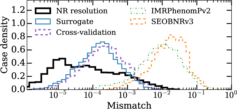
Figure 3: Mismatch histograms computed in the frequency domain with a flat power spectral density. The NR resolution mismatches compare waveforms from high and medium resolution NR simulations. This can be an overestimate of the error in the high resolution NR waveform, leading to some NR resolution mismatches being larger than the surrogate mismatches. We note that the IMRPhenomPv2 model does not contain all spin components.

We then compute mismatches using the advanced LIGO design sensitivity noise curve Shoemaker (2010); Aasi et al. (2015) using various total masses $M$. For each mass $M$, we obtain histograms as in Fig. 3, and we show the median and $95$th percentile mismatches from these histograms in Fig. 4. We note that for $M\lesssim 114M_{\odot}$ some or all waveforms begin above $10\,\mathrm{Hz}$ and do not cover the full design sensitivity frequency band. We find that the $95$th percentile mismatches of our surrogate model are similar to the corresponding NR mismatches, except for total masses above $160M_{\odot}$ where the NR mismatches are slightly smaller. The NRSur7dq2 surrogate yields mismatches at least an order of magnitude smaller than the other waveform models for all total masses investigated.

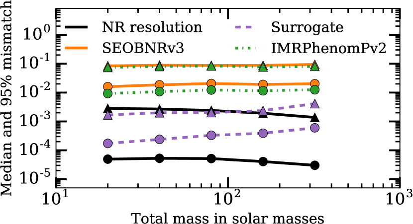
Figure 4: Median (circles) and $95$th percentile (triangles) mismatches of all $866$ cases computed with the advanced LIGO design sensitivity curve. The surrogate mismatches are computed using trial surrogates, as in the cross-validation curve of Fig. 3.

Figure 5 shows the real part of $h^{2,2}(t)$ for the cases leading to the largest mismatches in Fig. 3. The top panel shows the case leading to the largest surrogate cross-validation mismatch, and the bottom panel shows the case leading to the largest SEOBNRv3 mismatch. The surrogate waveforms shown are evaluated using the appropriate trial surrogate, so that they were not trained on the NR waveforms they are compared with. All waveforms are aligned to have their peak amplitude at $t=0$ and are rotated to have their orbital angular momentum aligned with the $z$ axis at $t=t_{0}=-4500M$. In the top panel, we see that both the SEOBNRv3 and surrogate waveforms have a similar phasing error around $t=-50M$. The phasing error of the surrogate does not grow significantly larger through merger and ringdown, so most of this error can be removed with a time and phase shift. For the SEOBNRv3 waveforms in both the upper and lower panels, the phasing error changes significantly during the merger; therefore this error does not decrease significantly even after performing a time and phase shift. In the top panel of Figure 5, the IMRPhenomPv2 waveform does as well as the surrogate; in the bottom panel, the IMRPhenomPv2 waveform has large errors in both phase and amplitude.

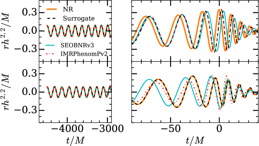
Figure 5: The real part of time domain waveforms for the case leading to the largest surrogate mismatch (top) and the largest SEOBNRv3 mismatch (bottom). The surrogate waveforms are evaluated using trial surrogates which were not trained with the NR waveform shown. The top panel uses SXS:BBH:0922 with $q\approx 2$, $\vec{\chi}_{1}(t_{0})\approx 0.8\hat{z}$, and $\vec{\chi}_{2}(t_{0})\approx-0.8\hat{y}$. The lower panel uses SXS:BBH:0900 with $q\approx 2$, $\vec{\chi}_{1}(t_{0})\approx(0.29,-0.74,0.02)$ and $\vec{\chi}_{2}(t_{0})\approx(0.43,-0.34,0.58)$.

VII Discussion and Conclusions

Within its range of validity, our NRSur7dq2 surrogate model is nearly as accurate as performing new NR simulations. The surrogate model takes only $\sim~{}50\,\mathrm{ms}$ to evaluate on a single CPU core, making it sufficiently fast for current GW data analysis applications such as parameter estimation. This evaluation time can be compared to $\mathcal{O}(\mathrm{weeks})$ on dozens of CPU cores to perform a new NR simulation, decreasing the cost in CPU-hours by $\mathcal{O}(10^{8})$. The NRSur7dq2 surrogate model data along with Python evaluation code is publicly available for download at SpE (b).

Our surrogate model is limited to mass ratios $q\leq 2$ and spin magnitudes $|\vec{\chi_{1,2}}|\leq 0.8$. While in principle the parametric fits can be extrapolated to more extreme mass ratios and spin magnitudes, we do not expect extrapolation to yield accurate waveforms. However, these limits can be extended in future versions of our surrogate model by performing NR simulations with larger mass ratios and spins.

Additionally, the waveforms produced by NRSur7dq2 are limited in duration to $4500M$ before the peak amplitude. This covers frequencies $f\geq 20\,\mathrm{Hz}$ for all systems with $M\gtrsim 57M_{\odot}$. For systems with lower total masses, or for systems with $M\lesssim 114M_{\odot}$ when including frequencies down to $10\,\mathrm{Hz}$, longer waveforms are needed. In future work, we plan to overcome this limitation by hybridizing with either PN or SEOBNRv3 Bustillo et al. (2015); Boyle (2011); Ohme et al. (2011); MacDonald et al. (2011), either by hybridizing the NR waveforms before building the surrogate or by hybridizing the surrogate waveforms. Longer NR waveforms would then be needed to test the accuracy of the hybridization step.

Appendix A Sparse grid parameters

We take the polar and azimuthal spin angles of the inertial frame spins $\vec{\chi}_{i}$ to be $\theta_{i}$ and $\phi_{i}$ respectively, for $i\in\{1,2\}$. We can then parametrize our $7$-dimensional parameter space by

• $q\in[1,2]$,

• $|\vec{\chi}_{i}|\in[0,0.8]$,

• $\theta_{i}\in[0,\pi]$,

• $\phi_{i}\in[0,2\pi]$.

The range of each of these variables is some closed interval $[a,b]$. For a variable $x$ with range $[a,b]$, we define a grid of $N$ uniformly-spaced points

$$g_{x}^{N}=\left\{a+\frac{n}{N-1}(b-a):n=0,\ldots,N-1\right\}\,,$$ (22)

where $N\geq 2$. We then define a sequence of grids

$$G_{x}\equiv G_{x}^{0},\,G_{x}^{1},\,\ldots\,,$$ (23)

where

$$G_{x}^{n}=g_{x}^{f_{x}(n)}$$ (24)

for some monotonically increasing function $f_{x}(n)$. We call $G_{x}^{n}$ the level $n$ grid for $x$. We take

$$f_{q}(n) =f_{|\vec{\chi_{i}}|}(n)=1+2^{n},$$ (25)

$$f_{\theta_{i}}(n) =1+2^{n+1},$$ (26)

$$f_{\phi_{i}}(n) =1+3\cdot 2^{n}\,.$$ (27)

These choices ensure that $G_{x}^{n}\subset G_{x}^{n+1}$, and that the level $0$ grids already give a description of the parameter space that does not leave out any phenomenology; the level $0$ grids for $\theta_{i}$ contain the midpoint $\pi/2$ leading to precession, and the level $0$ grids for $\phi_{i}$ contain $3$ unique points (since $\phi_{i}=0$ and $\phi_{i}=2\pi$ lead to the same physical spin) in order to get at least some resolution of features that behave like $\mathrm{sin}(\phi_{i}+\phi+0)$.

We have already seen that $\phi_{i}=0$ and $\phi_{i}=2\pi$ correspond to the same physical spin, but we will have many other scenarios where two combinations of variables lead to the same physical configuration. For example, if $|\vec{\chi}_{1}|=0$, all combinations of $\theta_{1}$ and $\phi_{1}$ lead to the same physical configuration. We will ignore these degenerate combinations for now, and remove them later on.

Dense grids in parameter space could be constructed as

$$G_{\mathrm{dense}}^{n}=G_{q}^{n}\times G_{|\vec{\chi}_{1}|}^{n}\times G_{\theta_{1}}^{n}\times G_{\phi_{1}}^{n}\times$$

$$G_{|\vec{\chi}_{2}|}^{n}\times G_{\theta_{2}}^{n}\times G_{\phi_{2}}^{n}\,,$$

where $\times$ denotes the Cartesian product. While the $1$-dimensional grids grow in size as $\mathcal{O}(2^{n})$, these dense grids grow in size as $\mathcal{O}(2^{7n})$ or as the seventh power of the size of the $1$-dimensional grids. This is known as the curse of dimensionality; the amount of data needed often grows exponentially with the dimensionality. Sparse grids Smolyak (1963); Bungartz and Griebel (2004) overcome the curse of dimensionality by using a sparse product such that the grids grow in size as $\mathcal{O}\left(2^{n}\left(\log 2^{n}\right)^{6}\right)$. If $G_{x}$ and $G_{y}$ are two sequences of grids, we define the sparse product of $G_{x}$ with $G_{y}$ to be $G_{x,y}=G_{x}\bullet G_{y}$, where

$$G_{x,y}^{n}=\bigcup\limits_{k=0}^{n}G_{x}^{k}\times G_{y}^{n-k}\,.$$ (28)

We now define the sparse grids for our parameter space from the sequence of grids

$$G=G_{q}\bullet G_{|\vec{\chi}_{1}|}\bullet G_{\theta_{1}}\bullet G_{\phi_{1}}\bullet G_{|\vec{\chi}_{2}|}\bullet G_{\theta_{2}}\bullet G_{\phi_{2}}$$ (29)

such that

$$G^{n}=\bigcup\limits_{\sum_{i=1}^{7}k_{i}=n}G_{q}^{k_{1}} \times G_{|\vec{\chi}_{1}|}^{k_{2}}\times G_{\theta_{1}}^{k_{3}}\times G_{\phi_{1}}^{k_{4}}$$

$$\times G_{|\vec{\chi}_{2}|}^{k_{5}}\times G_{\theta_{2}}^{k_{6}}\times G_{\phi_{2}}^{k_{7}}\,.$$

Starting with the parameters in $G^{1}$ we removed physically identical configurations. We also removed configurations with $\vec{\chi}_{2}\propto\hat{z}$, which are within the parameter space of the NRSur4d2s surrogate model, which was already covered by the $276$ NRSur4d2s NR simulations. We performed $361$ new NR simulations based on the remaining set of parameter values.

Appendix B Time sampling

We wish to choose time nodes $t_{0}<t_{1}<\ldots<t_{f}$ that are roughly uniformly spaced in the orbital phase $\varphi(t)$ for all cases. Given some number $N$, we choose time nodes yielding roughly $N$ nodes per orbit. Since different NR waveforms have different orbital frequencies, they will have a different number of time nodes per orbit. Our scheme for choosing the time nodes given $N$ is based on the leading order PN expression for the orbital angular frequency $\omega(t)$ during the inspiral, smoothly transitioning to a maximum value of $\omega=2\pi/(20M)$ during the ringdown. We do this by computing a bounded time

$$\tilde{t}(t)=-1.7+\frac{1}{2}\left((t+5)-\sqrt{(t+5)^{2}+25}\right)\,,$$ (30)

and then choosing

$$\omega_{\mathrm{ref}}(t)=\omega_{\mathrm{0PN}}(\tilde{t}(t))=\left(\frac{64}{5}(-\tilde{t}(t))\right)^{-\frac{3}{8}}\,.$$ (31)

We then use spacings between nodes $t_{j+1}-t_{j}=\omega_{\mathrm{ref}}(t_{j})$.

Appendix C Fourth-order Adams-Bashforth method

We integrate the ODE system on a non-uniformly spaced grid of time nodes $t_{0}<t_{1}<\ldots<t_{f}$ using a fourth-order Adams-Bashforth scheme Butcher (2003); Bashforth and Adams (1883). We denote the solution $\vec{y}(t)$, and at each time node $t_{i}$, we can evaluate fits to determine

$$\frac{d\vec{y}}{dt}=\vec{f}(t;\vec{y})\,.$$ (32)

We first integrate up to $t_{3}$ using a Runge-Kutta fourth-order scheme.

Once we have integrated up to $t_{i}$ for $i>=3$, we have previously evaluated

$$\vec{k}_{j}=\vec{f}(t_{j};\vec{y}(t_{j}))$$ (33)

for $0\leq j<i$, and we now evaluate $\vec{k}_{i}$. We approximate $\vec{g}(t)=\vec{f}(t;\vec{y}(t))$ by a cubic function

$$\vec{g}(t)\approx\vec{g}_{3}(t)=\vec{A}+\vec{B}(t-t_{i})+\vec{C}(t-t_{i})^{2}+\vec{D}(t-t_{i})^{3}\,.$$ (34)

The coefficients are chosen such that $\vec{g}_{3}(t_{j})=\vec{g}(t_{j})=\vec{k}_{j}$ for $i-3\leq j\leq i$, giving $\vec{A}=\vec{k}_{i}$, and

$$\begin{bmatrix}\vec{B}\\ \vec{C}\\ \vec{D}\\ \end{bmatrix}=\begin{bmatrix}\frac{\delta_{-1,0}\delta_{-2,0}}{\Delta_{1}}&\frac{\delta_{-1,0}\delta_{-3,0}}{\Delta_{2}}&\frac{\delta_{-2,0}\delta_{-3,0}}{\Delta_{3}}\\ \frac{\delta_{-2,0}+\delta_{-1,0}}{\Delta_{1}}&\frac{\delta_{-1,0}+\delta_{-3,0}}{\Delta_{2}}&\frac{\delta_{-2,0}+\delta_{-3,0}}{\Delta_{3}}\\ \frac{1}{\Delta_{1}}&\frac{1}{\Delta_{2}}&\frac{1}{\Delta_{3}}\end{bmatrix}\begin{bmatrix}\vec{k}_{i}-\vec{k}_{i-3}\\ \vec{k}_{i}-\vec{k}_{i-2}\\ \vec{k}_{i}-\vec{k}_{i-1}\end{bmatrix}\,.$$

Here, $\delta_{n,m}=t_{i+m}-t_{i+n}$ and

$$\Delta_{1} =\delta_{-3,-2}\delta_{-3,-1}\delta_{-3,0}\,,$$ (35)

$$\Delta_{2} =\delta_{-3,-2}\delta_{-2,-1}\delta_{-2,0}\,,$$ (36)

$$\Delta_{3} =\delta_{-2,-1}\delta_{-3,-1}\delta_{-1,0}\,.$$ (37)

Finally, we approximate

$$\vec{y}(t_{i+1}) =\vec{y}(t_{i})+\int_{t_{i}}^{t_{i+1}}g(t)dt$$

$$\approx\vec{y}(t_{i})+\int_{t_{i}}^{t_{i+1}}g_{3}(t_{j})dt$$

$$=\vec{y}(t_{i})+\delta_{0,1}\vec{A}+\frac{1}{2}\delta_{0,1}^{2}\vec{B}+\frac{1}{3}\delta_{0,1}^{3}\vec{C}+\frac{1}{4}\delta_{0,1}^{4}\vec{D}\,.$$

References

References

- Abbott et al. (2016a) B. P. Abbott et al. (LIGO Scientific Collaboration, Virgo Collaboration), Phys. Rev. Lett. 116, 061102 (2016a), arXiv:1602.03837 [gr-qc] .
- Abbott et al. (2016b) B. P. Abbott et al. (LIGO Scientific Collaboration, Virgo Collaboration), Phys. Rev. Lett. 116, 241103 (2016b), arXiv:1606.04855 [gr-qc] .
- Abbott et al. (2016c) B. P. Abbott et al. (LIGO Scientific Collaboration, Virgo Collaboration), Phys. Rev. Lett. 116, 241102 (2016c), arXiv:1602.03840 [gr-qc] .
- Abbott et al. (2016d) B. P. Abbott et al. (LIGO Scientific Collaboration, Virgo Collaboration), Phys. Rev. D 94, 064035 (2016d), arXiv:1606.01262 [gr-qc] .
- Abbott et al. (2016e) B. P. Abbott et al. (LIGO Scientific Collaboration, Virgo Collaboration), Phys. Rev. Lett. 116, 221101 (2016e), arXiv:1602.03841 [gr-qc] .
- Pretorius (2005) F. Pretorius, Phys. Rev. Lett. 95, 121101 (2005), arXiv:gr-qc/0507014 [gr-qc] .
- Zlochower et al. (2005) Y. Zlochower, J. Baker, M. Campanelli, and C. Lousto, Phys. Rev. D 72, 024021 (2005), arXiv:gr-qc/0505055 [gr-qc] .
- SpE (a) http://www.black-holes.org/SpEC.html (a).
- (9) Einstein Toolkit home page: http://einsteintoolkit.org.
- Husa et al. (2008) S. Husa, J. A. González, M. Hannam, B. Brügmann, and U. Sperhake, Class. Quantum Grav. 25, 105006 (2008).
- Brügmann et al. (2008) B. Brügmann, J. A. González, M. Hannam, S. Husa, U. Sperhake, and W. Tichy, Phys. Rev. D 77, 024027 (2008), gr-qc/0610128 .
- Herrmann et al. (2007) F. Herrmann, I. Hinder, D. Shoemaker, and P. Laguna, Class. Quantum Grav. 24, S33 (2007), gr-qc/0601026 .
- Damour et al. (2008) T. Damour, P. Jaranowski, and G. Schaefer, Phys. Rev. D 78, 024009 (2008), arXiv:0803.0915 [gr-qc] .
- Damour and Nagar (2009) T. Damour and A. Nagar, Phys. Rev. D 79, 081503 (2009), arXiv:0902.0136 [gr-qc] .
- Taracchini et al. (2014) A. Taracchini, A. Buonanno, Y. Pan, T. Hinderer, M. Boyle, D. A. Hemberger, L. E. Kidder, G. Lovelace, A. H. Mroue, H. P. Pfeiffer, M. A. Scheel, B. Szilágyi, N. W. Taylor, and A. Zenginoglu, Phys. Rev. D 89 (R), 061502 (2014), arXiv:1311.2544 [gr-qc] .
- Pürrer (2016) M. Pürrer, Phys. Rev. D 93, 064041 (2016), arXiv:1512.02248 [gr-qc] .
- Pan et al. (2013) Y. Pan, A. Buonanno, A. Taracchini, L. E. Kidder, A. H. Mroué, H. P. Pfeiffer, M. A. Scheel, and B. Szilágyi, Phys. Rev. D 89, 084006 (2013), arXiv:1307.6232 [gr-qc] .
- Bohé et al. (2017) A. Bohé, L. Shao, A. Taracchini, A. Buonanno, S. Babak, I. W. Harry, I. Hinder, S. Ossokine, M. Pürrer, V. Raymond, T. Chu, H. Fong, P. Kumar, H. P. Pfeiffer, M. Boyle, D. A. Hemberger, L. E. Kidder, G. Lovelace, M. A. Scheel, and B. Szilágyi, Phys. Rev. D 95, 044028 (2017), arXiv:1611.03703 [gr-qc] .
- Hannam et al. (2014) M. Hannam, P. Schmidt, A. Bohé, L. Haegel, S. Husa, et al., Phys. Rev. Lett. 113, 151101 (2014), arXiv:1308.3271 [gr-qc] .
- Khan et al. (2016) S. Khan, S. Husa, M. Hannam, F. Ohme, M. Pürrer, X. Jiménez Forteza, and A. Bohé, Phys. Rev. D93, 044007 (2016), arXiv:1508.07253 [gr-qc] .
- Husa et al. (2016) S. Husa, S. Khan, M. Hannam, M. Pürrer, F. Ohme, X. Jiménez Forteza, and A. Bohé, Phys. Rev. D93, 044006 (2016), arXiv:1508.07250 [gr-qc] .
- Lindblom et al. (2008) L. Lindblom, B. J. Owen, and D. A. Brown, Phys. Rev. D 78, 124020 (2008), arXiv:0809.3844 [gr-qc] .
- Abbott et al. (2016f) B. P. Abbott et al. (Virgo, LIGO Scientific), (2016f), arXiv:1611.07531 [gr-qc] .
- Blackman et al. (2017) J. Blackman, S. E. Field, M. A. Scheel, C. R. Galley, D. A. Hemberger, P. Schmidt, and R. Smith, (2017), arXiv:1701.00550 [gr-qc] .
- Blackman et al. (2015) J. Blackman, S. E. Field, C. R. Galley, B. Szilágyi, M. A. Scheel, M. Tiglio, and D. A. Hemberger, Phys. Rev. Lett. 115, 121102 (2015), arXiv:1502.07758 [gr-qc] .
- Field et al. (2014) S. E. Field, C. R. Galley, J. S. Hesthaven, J. Kaye, and M. Tiglio, Phys. Rev. X 4, 031006 (2014), arXiv:1308.3565 [gr-qc] .
- Pürrer (2014) M. Pürrer, Class. Quantum Grav. 31, 195010 (2014), arXiv:1402.4146 [gr-qc] .
- Pfeiffer et al. (2003) H. P. Pfeiffer, L. E. Kidder, M. A. Scheel, and S. A. Teukolsky, Comput. Phys. Commun. 152, 253 (2003), gr-qc/0202096 .
- Lovelace et al. (2008) G. Lovelace, R. Owen, H. P. Pfeiffer, and T. Chu, Phys. Rev. D 78, 084017 (2008).
- Lindblom et al. (2006) L. Lindblom, M. A. Scheel, L. E. Kidder, R. Owen, and O. Rinne, Class. Quantum Grav. 23, S447 (2006), gr-qc/0512093 .
- Szilágyi et al. (2009) B. Szilágyi, L. Lindblom, and M. A. Scheel, Phys. Rev. D 80, 124010 (2009), arXiv:0909.3557 [gr-qc] .
- M. A. Scheel, M. Boyle, T. Chu, L. E. Kidder, K. D. Matthews and H. P. Pfeiffer (2009) M. A. Scheel, M. Boyle, T. Chu, L. E. Kidder, K. D. Matthews and H. P. Pfeiffer, Phys. Rev. D 79, 024003 (2009), arXiv:gr-qc/0810.1767 .
- Szilágyi (2014) B. Szilágyi, Int. J. Mod. Phys. D 23, 1430014 (2014), arXiv:1405.3693 [gr-qc] .
- Boyle and Mroué (2009) M. Boyle and A. H. Mroué, Phys. Rev. D 80, 124045 (2009), arXiv:0905.3177 [gr-qc] .
- Boyle (2016) M. Boyle, Phys. Rev. D 93, 084031 (2016).
- Boyle (2013) M. Boyle, Phys. Rev. D 87, 104006 (2013).
- Boyle et al. (2014) M. Boyle, L. E. Kidder, S. Ossokine, and H. P. Pfeiffer, (2014), arXiv:1409.4431, arXiv:1409.4431 .
- (38) “Scri,” https://github.com/moble/scri.
- Ossokine et al. (2015) S. Ossokine, M. Boyle, L. E. Kidder, H. P. Pfeiffer, M. A. Scheel, and B. Szilágyi, Phys. Rev. D 92, 104028 (2015), arXiv:1502.01747 [gr-qc] .
- Boyle et al. (2011) M. Boyle, R. Owen, and H. P. Pfeiffer, Phys. Rev. D 84, 124011 (2011), arXiv:1110.2965 [gr-qc] .
- Aylott et al. (2009) B. Aylott, J. G. Baker, W. D. Boggs, M. Boyle, P. R. Brady, et al., Class. Quantum Grav. 26, 165008 (2009), arXiv:0901.4399 [gr-qc] .
- Smolyak (1963) S. A. Smolyak, in Dokl. Akad. Nauk SSSR, Vol. 4 (1963) p. 123.
- Bungartz and Griebel (2004) H.-J. Bungartz and M. Griebel, Acta numerica 13, 147 (2004).
- Schmidt et al. (2011) P. Schmidt, M. Hannam, S. Husa, and P. Ajith, Phys. Rev. D 84, 024046 (2011), arxiv:1012.2879 .
- O’Shaughnessy et al. (2011) R. O’Shaughnessy, B. Vaishnav, J. Healy, Z. Meeks, and D. Shoemaker, Phys. Rev. D 84, 124002 (2011), arXiv:1109.5224 .
- Blanchet (2014) L. Blanchet, Living Rev. Rel. 17, 2 (2014).
- Butcher (2003) J. C. Butcher, Numerical Methods for Ordinary Differential Equations (Wiley, 2003).
- Bashforth and Adams (1883) F. Bashforth and J. C. Adams, An attempt to test the theories of capillary action by comparing the theoretical and measured forms of drops of fluid (Cambridge University Press, 1883).
- SpE (b) http://www.black-holes.org/surrogates/ (b).
- Babak et al. (2017) S. Babak, A. Taracchini, and A. Buonanno, Phys. Rev. D95, 024010 (2017), arXiv:1607.05661 [gr-qc] .
- Shoemaker (2010) D. Shoemaker (LIGO Collaboration), “Advanced LIGO anticipated sensitivity curves,” (2010), LIGO Document T0900288-v3.
- Aasi et al. (2015) J. Aasi et al. (LIGO Scientific Collaboration), Class. Quantum Grav. 32, 074001 (2015), arXiv:1411.4547 [gr-qc] .
- Bustillo et al. (2015) J. C. Bustillo, A. Bohé, S. Husa, A. M. Sintes, M. Hannam, et al., (2015), arXiv:1501.00918 [gr-qc] .
- Boyle (2011) M. Boyle, Phys. Rev. D 84, 064013 (2011).
- Ohme et al. (2011) F. Ohme, M. Hannam, and S. Husa, Phys. Rev. D 84, 064029 (2011).
- MacDonald et al. (2011) I. MacDonald, S. Nissanke, and H. P. Pfeiffer, Class. Quantum Grav. 28, 134002 (2011), arXiv:1102.5128 [gr-qc] .