CacheShuffle: An Oblivious Shuffle Algorithm using Caches

Abstract

We consider the problem of Oblivious Shuffling, a critical component in several applications in which one wishes to hide the pattern of data access, and the problem of $K$-Oblivious Shuffling, a refinement thereof. We provide efficient algorithms for both problems and discuss their application to the design of Oblivious RAM. The task of a $K$-Oblivious Shuffling algorithm is to obliviously shuffle $N$ encrypted blocks that have been randomly allocated on the server in such a way that an adversarial server learns nothing about the new allocation of blocks. The security guarantee should hold also with respect to an adversary that has learned the initial position of $K$ touched blocks out of the $N$ blocks. The classical notion of Oblivious Shuffling is obtained for $K=N$.

We start by presenting a family of algorithms for Oblivious Shuffling. Our first construction, that we call ${\sf CacheShuffle}{\sf Root}$, is tailored for clients with $O(\sqrt{N})$ blocks of memory and uses $(4+\epsilon)N$ blocks of bandwidth, for every $\epsilon>0$ and has negligible in $N$ failure probability. ${\sf CacheShuffle}{\sf Root}$ is a 4.5x improvement over the previous best known result on practical sizes of $N$. We also present ${\sf CacheShuffle}$ that obliviously shuffles using $O(S)$ blocks of client memory with $O(N\log_{S}N)$ blocks of bandwidth.

We then turn to $K$-Oblivious Shuffling and give algorithms that require $2N+f(K)$ blocks of bandwidth, for some function $f$. That is, any extra bandwidth above the $2N$ lower bound depends solely on $K$. We present ${\sf K}{\sf CacheShuffle}{\sf Basic}$ that uses $O(K)$ client storage and exactly $2N$ blocks of bandwidth. For smaller client storage requirements, we show ${\sf K}{\sf CacheShuffle}$, which uses $O(S)$ client storage and requires $2N+(1+\epsilon)O(K\log_{S}K)$ blocks of bandwidth.

Finally, motivated by applications to ORAM design, we consider also the case in which, in addition to the $N$ blocks, the server stores $D$ dummy blocks whose content is is irrelevant but still their positions must be hidden by the shuffling. For this case, we design algorithm KCacheShuffleDummy that, for $N+D$ blocks and $K$ touched blocks, uses $O(K)$ client storage and $D+(2+\epsilon)N$ blocks of bandwidth.

We discuss how to use KCacheShuffleBasic and KCacheShuffleDummy to improve practical Oblivious RAM constructions.

1 Introduction

Cloud storage has become an increasingly popular technology due to the many benefits it offers users. Uploading files to the cloud allows users to share documents easily without incurring into bandwidth costs or the annoyance of email attachments. Users are able to access documents from anywhere without having to transfer data between machines. The burden of replicating data and recovering from machine failures is placed on the storage provider. For many corporations, cloud storage becomes cost efficient since the price of cloud storage may be cheaper than developing and maintaining their own internal storage systems.

Some users might want to hide the contents of their data from their cloud providers. A first attempt would be to encrypt all documents by the client before uploading the files to the server. Work done in [12] and [15] show that the access pattern to encrypted data may leak information to cloud storage providers. Data oblivious algorithms and storage can be used to hide the access pattern to remote data with Oblivious Random Access Memory (ORAM) being the primary example. ORAM was first introduced by [5] (see also [6]) that introduced the so called Square Root ORAM (with a square root communication overhead and client memory) and the Hierarchical ORAM construction which has poly-logarithmic amortized cost and sublinear client storage. Recently, more practical constructions such as Path ORAM [22], Partition ORAM [21] and Recursive Square Root ORAM [18] have appeared. The best known asymptotic results with $O(\log N)$ amortized query cost with $O(N^{\epsilon})$ blocks of client storage was first shown in [10]. The result was improved to make the worst case also $O(\log N)$ in [9]. However, these asymptotic results have constants too large to be considered practical at the moment.

Many ORAM constructions have amortized costs due to the need of periodically running an oblivious shuffling algorithm. Roughly speaking, an oblivious shuffle moves around the data blocks in such a way that the server cannot link together the position of a block before the shuffle with the position of the same block after the shuffle. This is used to completely remove any links that the server might have created with the data blocks in the position before the oblivious shuffle. Essentially, all extracted information is rendered useless. This idea appeared in the original Square Root ORAM and Hierarchical ORAM that allowed clients to perform accesses until a break point was reached where the server might be able to extract extra information from the access pattern. At this point, the client performs an oblivious shuffle (after which, new queries cannot provide extra information to the server), and queries can occur again.

The early approach to oblivious shuffling involved the use of sorting circuits (or of oblivious sorting algorithms that can also be seen as sorting circuits). The client evaluates the compare-exchange gates one at a time and for each gate it downloads the two encrypted blocks that are input to the gate, re-encrypts them and uploads them in right order. Batcher’s sort is considered the most practical algorithm [2] even though it has asymptotic cost of $O(N\log^{2}N)$. Sorting networks such as AKS [1] and Zig-Zag [8] have $O(N\log N)$ size, but are considered impractical due to large constants. Randomized Shellsort [7] has larger depth than AKS but the constant hidden in the big Oh notation is smaller. Oblivious shuffling based on sorting circuits is interesting because the client need only to store a constant number of data blocks but it requires bandwidth proportional to the size of the network which is $\Omega(N\log N)$. The first oblivious shuffling algorithm not based on sorting circuits, the Melbourne Shuffle, was introduced in [16] and uses $O(N)$ bandwidth while only requiring $O(\sqrt{N})$ blocks to be stored on the client at any time.

Results and Contributions.

In this paper, we present practical algorithms for oblivious shuffling.

We base our design on the following observation that has been overlooked by previous work. As we have discussed, the main goal of oblivious shuffling is to make sure that the adversary cannot accumulate too much information on which slot in server memory holds which block in algorithms that hide the access pattern to data blocks. However, it is seldom the case that the adversary gets to learn the position of all the $N$ blocks but, rather, of a number of blocks that is equal to the size of the client memory. In addition, the client knows exactly which blocks have been touched by the server. We call these blocks the touched blocks. This is the case, for example, for the Square Root ORAM of [5, 6] and of its hierarchical versions. Motivated by this observation, we introduce the concept of a $K$-Oblivious Shuffling Algorithm that reshuffles $N$ data blocks, $K$ of which are touched. For $K=N$, the notions of a $K$-Oblivious Shuffling Algorithm coincides with the original notion of an Oblivious Shuffling Algorithm of [16].

Before tackling the problem of designing efficient $K$-Oblivious Shuffling Algorithms, we revisit the original Oblivious Shuffling problem by providing improved algorithms. All our algorithms use a cache in client memory to store blocks downloaded from the server before they can be uploaded to the server. The main technical difficulty is to show that the cache does not grow too much. We first apply this design principle in Section 4 by presenting an Oblivious Shuffling Algorithm, ${\sf CacheShuffle}{\sf Root}$, that uses bandwidth $(4+\epsilon)N$ and client memory $O(\sqrt{N})$ and has negligible failure probability. For similar client memory usage and error probability, Melbourne Shuffle [16] uses about 4 times more bandwidth. We generalize this construction to ${\sf CacheShuffle}$ in Section 5 to any client memory $S=\omega(\log N)$ in which case bandwidth is $O(N\log N/\log S)$ and probability of failure is still negligible.

We then turn to the design of $K$-Oblivious Shuffling Algorithms for $K\leq N$. From a high level, the number $K$ of touched data blocks succinctly describes the difficulty of shuffling the specific data sets. In the extreme case that no block has been disclosed (e.g., in an ORAM in which no query has been performed), clearly no shuffle is required. On the other hand, if all blocks have been touched, then oblivious shuffling becomes hardest. All previous oblivious shuffling algorithms have always considered the most difficult scenario and have reshuffled so to guarantee security as if all the blocks had been touched, even if that was not the case in the specific application. Our work is the first to separate the two problems. In Section 6, we give a simple $K$-Oblivious Shuffling Algorithm ${\sf K}{\sf CacheShuffle}{\sf Basic}$ for the case in which client memory $S\geq K$. This setting is relevant to ORAM design and, for every $K$, we obtain an algorithm with bandwidth $2N$. In Section 7, we give, for every client memory $S=\omega(\log N)$ and for every $\epsilon$, algorithm ${\sf K}{\sf CacheShuffle}$ that uses bandwidth $2N+c\cdot(1+\epsilon)K\log_{S}K$, for constant $c$. For the special case of $S=\sqrt{K}$, we have algorithm ${\sf K}{\sf CacheShuffle}{\sf Root}$ that uses bandwidth $2N+(4+\epsilon)K$. For every $\epsilon>0$, the algorithms have negligible in $N$ abort probability.

Motivated by the problem of designing bandwidth efficient ORAM, in Section 8 we consider a scenario in which there are $D$ dummy blocks, which can be of arbitrary values, in addition to $N$ real blocks. It is possible to use any $K$-Oblivious Shuffling Algorithm in this scenario and just treat the dummy blocks as any other block. By taking into account instead the fact that the content of the dummy blocks is irrelevant we present algorithm KCacheShuffleDummy that has bandwidth of $D+2(N+\epsilon)$ blocks for some small $\epsilon>0$ for the case in which $S\geq K$. Applying directly ${\sf K}{\sf CacheShuffle}{\sf Basic}$ would result in bandwidth $2(N+D)$ and so we are saving bandwidth corresponding to $D$ blocks. The savings come at the cost of a small amount of server computation,

In the table below, we compare our algorithms with the previous best algorithm for Oblivious Shuffling, Melbourne Shuffle [16].

	Client Storage	Bandwidth
Melbourne Shuffle [16]	$O(\sqrt{N})$	$\approx 18N$
CacheShuffleRoot	$O(\sqrt{N})$	$(4+\epsilon)N$
CacheShuffle	$O(S)$	$O(N\log_{S}N)$
KCacheShuffleBasic	$O(K)$	$2N$
KCacheShuffleRoot	$O(\sqrt{K})$	$2N+(4+\epsilon)K$
KCacheShuffle	$O(S)$	$2N+(1+\epsilon)O(K\log_{S}K)$
KCacheShuffleDummy	$O(K)$	$D+(2+\epsilon)N$

Figure 1: $N$ denotes the number of blocks. Algorithm KCacheShuffleDummy receives $D$ additional dummy blocks, for a total of $N+D$ blocks. Algorithm KCacheShuffleRoot is obtained from algorithm KCacheShuffle by setting $S=\sqrt{N}$. For all algorithms, server storage is $c\cdot N$, for small constant $c$.

2 Definitions

Our reference scenario is a cloud storage model with a client that wishes to outsource the storage of $N$ data blocks of identical sizes to a server that has storage of capacity $M\geq N$. In this context, we consider the problem of obliviously shuffling the data blocks.

We assume that the data blocks have been uploaded by the Setup algorithm that takes as input a sequence ${\mathbb{B}}=(B_{1},\ldots,B_{N})$ of $N$ data blocks of identical sizes $B$ and a permutation $\pi:[N]\rightarrow[N]$. The Setup algorithm randomly selects an encryption key ${\mathtt{key}}$ for a symmetric encryption scheme and uploads the data blocks encrypted using ${\mathtt{key}}$ to the server by storing it in the first $N$ locations of the server storage according to $\pi$; that is, if $\pi(i)=j\in[N]$, an encrypted copy of the $i$-th data block is stored at the $j$-th location of the server storage. Note that $\pi$ is a permutation and each of the $N$ data blocks is uploaded exactly once to the server.

Once the data has been uploaded, an adversary ${{\mathcal{A}}}$ is allowed to query for the position of a subset ${\mathsf{Touched}}$ of the data blocks and for each queried block $i$, the value $\pi(i)$ is revealed to ${{\mathcal{A}}}$. We call the data blocks in ${\mathsf{Touched}}$, the touched data blocks.

The Shuffling algorithm, instead, takes as input the encryption key ${\mathtt{key}}$ used to setup the $N$ blocks, the permutation map $\pi$, the set ${\mathsf{Touched}}$ of touched data blocks and a new permutation $\sigma$. The task of the Shuffling algorithm is to re-permute the $N$ data blocks stored on the server according to permutation map $\sigma$. At each step, the Shuffling algorithm can download a block $i$ to client memory by specifying the block’s current location on the server or upload a block from client memory to server memory by specifying its destination on the server. In addition, the Shuffling algorithm can ask the server to perform operation on locally stored data blocks. We are interested in oblivious Shuffling algorithms that, roughly speaking, have the property of hiding information about the content of the data blocks and on $\sigma$, even to an adversarial algorithm that has partial information on $\pi$ (the set ${\mathsf{Touched}}$) and observes the blocks downloaded and uploaded by the Shuffling algorithm.

The mechanics of the Shuffling algorithm.

A Shuffling algorithm receives as input the initial permutation $\pi$, the final permutation $\pi$ and the set ${\mathsf{Touched}}$. The Shuffling algorithm proceeds in steps and each step can be either a move step or a server computation step. The state after the $q$-th step is described by a server allocation map $\rho_{q}:[M]\rightarrow[N]\cup\{\perp\}$ and by a client allocation map $L_{q}:[S]\rightarrow[N]\cup\{\perp\}$. Each allocation map specify the block in each of the $M$ server locations and $S$ client locations, respectively. More precisely, $\rho_{q}(j)=i$ means that, after the $q$-th step is performed, the $j$-th server location contains an encryption of the $i$-th data block. If instead $\rho_{q}(j)=\perp$, then an encryption of a dummy data block is stored at location $j$. Note that, unlike permutations, the argument of an allocation map is an index of a slot in memory and its value is a block index. Similarly statements are true for the client allocation map but $L_{q}(j)=\perp$ denotes an empty client slot.

When a Shuffling algorithm starts, the server allocation map $\rho_{0}$ coincides with permutation map $\pi$ on the first $N$ storage location of the $M$ server memory locations and has dummy blocks on the remaining $N-M$ locations; that is, for $1\leq i\leq N$, $\rho_{0}(i)=\pi^{-1}(i)$ and $\rho_{0}(i)=\perp$, for $i>N$. Instead $L_{0}[i]=\perp$ for all $i\in[S]$ (that is, initially, no block is stored in the client’s local memory). At each step, a Shuffling algorithm can perform either a move operation or a server computation operation. A move operation can be either a download or an upload move and they modify the state as follows. If the $q$-th move is a download move with source $s_{q}$ and destination $d_{q}$, it has the effect of storing an encryption of block $\rho_{q-1}(s_{q})$ stored at server location $s_{q}$ at location $L_{q}(d_{q})$ of the client memory; that is, the block at location $s_{q}$ on the server is downloaded, decrypted using ${\mathtt{key}}$ and re-encrypted by using ${\mathtt{key}}$ and fresh randomness. As a consequence, the server allocation map stays the same $\rho_{q}:=\rho_{q-1}$ and $L_{q}$ is the same as $L_{q-1}$ with the exception that $L_{q}(d_{q})=\rho_{q-1}(s_{q})$. If instead, the $q$-th move is an upload move with source $s_{q}$ and destination $d_{q}$, it has the effect of uploading the block in client location $s_{l}$ to server location $d_{q}$; that is, the client allocation map stays the same $S_{q}:=S_{q-1}$ and $\rho_{q}$ differs from $\rho_{q-1}$ only for the values at $d_{q}$. Our algorithms will also use special upload moves with $s_{q}=\perp$ in which a dummy block (say, a block consisting of all $0$’s) is uploaded to server location $d_{q}$. A server computation operation is instead specified by a circuit that takes as input a subset of the blocks and modifies the blocks stored at the server. As we shall see, this operation consists of homomorphic operation on ciphertext and can be used to save bandwidth while requiring more server computation. can also perform operations on blocks stored on the server in which case the length of the description of the circuit describing the operation is added to the bandwidth. We compute the bandwidth of a Shuffling algorithm using the block size $B$ as a unit of measurement; thus bandwidth is simply the number of move operations plus the size of the circuits corresponding to server computation operations divided by $B$.

Efficiency measures.

Three measures of efficiency can be considered for a Shuffling algorithm: the total bandwidth $T$, the amount $S$ of client memory and the amount $M$ of server memory. Note that oblivious shuffling of $N$ data blocks is trivial for clients with memory $S\geq N$: download all the $N$ encrypted blocks in some fixed order; decrypt and re-encrypt each block; finally, upload the newly encrypted blocks to the new locations one by one in some fixed order.

In this paper, we give oblivious shuffling algorithms that use memory $S=o(N)$ and server memory $M=O(N)$. In most cases, server memory is cheaper than block transfers, so we do not try to optimize for the hidden constants of server memory (which is however small for all our constructions). Our main objective is to design algorithms with small $T$.

The security notion.

A transcript of an execution of a Shuffling algorithm ${{\mathsf{Sh}}}$ consists of the initial content of the server memory, the ordered list of the sources of all download moves, the ordered list of the destinations of all the upload moves as well as the data blocks uploaded with each move, and the list of circuits uploaded by the client. We stress that a transcript only contains the server locations that are involved in each move (that is the source for the downloads and the destination for the uploads) but not the client locations so to model the fact that an adversarial server ${{\mathcal{A}}}$ cannot observe where each block is stored when downloaded and from which client location each uploaded block comes from.

For every sequence of $N$ blocks ${\mathbb{B}}=(B_{1},\ldots,B_{N})$, every subset ${\mathsf{Touched}}$ of touched blocks, and every pair of permutations $(\pi,\sigma)$, a Shuffling algorithm ${{\mathsf{Sh}}}$ naturally induces a probability distribution ${{\mathcal{T}}}_{{{\mathsf{Sh}}}}({\mathbb{B}},\pi,\sigma,{\mathsf{Touched}})$ over all possible transcripts. We capture the notion of a $K$-Oblivious Shuffling algorithm by the following game $\mathsf{OSGame}^{{\mathcal{A}}}_{{\mathsf{Sh}}}$ for Shuffling algorithm ${{\mathsf{Sh}}}$ between an adversary ${{\mathcal{A}}}$ and the challenger ${{\mathcal{C}}}$. In the formalization of our notion of security, we allow the adversary ${{\mathcal{A}}}$ to receive partial information on the starting permutation map $\pi$ to reflect the fact that the Shuffling algorithm ${{\mathsf{Sh}}}$ might be part of a larger protocol whose execution leaks information on $\pi$. More precisely, in our formalization we allow ${{\mathcal{A}}}$ to choose the initial location on the server of a subset ${\mathsf{Touched}}$ of the $N$ data blocks and we parametrize the security notion by the cardinality $K$ of the set ${\mathsf{Touched}}$. The challenger ${{\mathcal{C}}}$ fills in the remaining $N-K$ locations randomly under the constraint that each of the $N$ blocks appears in exactly one location on the server. Then, ${{\mathcal{A}}}$ proposes two sequences, ${\mathbb{B}}_{0}$ and ${\mathbb{B}}_{1}$, of $N$ blocks and two permutations, $\sigma_{0}$ and $\sigma_{1}$, and ${{\mathcal{C}}}$ randomly picks $b\in\{0,1\}$ and samples a transcript ${\mathcal{M}}^{{{\mathsf{Sh}}}}(\operatorname{\text{\sf Enc}}(K,{\mathbb{B}}_{b}),\pi,\sigma_{b},{\mathsf{Touched}})$ according to ${{\mathcal{T}}}^{{{\mathsf{Sh}}}}(\operatorname{\text{\sf Enc}}(K,{\mathbb{B}}_{b}),\pi,\sigma_{b},{\mathsf{Touched}})$. ${{\mathcal{A}}}$ then, on input ${\mathtt{trans}}$, outputs its guess $b^{\prime}$ for $b$. We say that an adversary ${{\mathcal{A}}}$ is $K$-restricted if it specifies the location of at most $K$ blocks; that is $|{\mathsf{Touched}}|\leq K$.

Definition 2.1.

For shuffle algorithm ${{\mathsf{Sh}}}$ and adversary ${{\mathcal{A}}}$, we define game $\mathsf{OSGame}^{{\mathcal{A}}}_{{{\mathsf{Sh}}}}(N,\lambda)$ as follows

1. ${{\mathcal{A}}}$ chooses a subset ${\mathsf{Touched}}\subseteq[N]$ and specifies $\pi(i)$ for each $i\in{\mathsf{Touched}}$;

2. ${{\mathcal{A}}}$ chooses two pairs $({\mathbb{B}}_{0},\sigma_{0})$ and $({\mathbb{B}}_{1},\sigma_{1})$ and sends them to ${{\mathcal{C}}}$;

3. ${{\mathcal{C}}}$ completes the permutation $\pi$ by randomly choosing the values at the point left unspecified by ${{\mathcal{A}}}$;

4. ${{\mathcal{C}}}$ randomly selects $b\leftarrow\{0,1\}$ and sends ${{\mathcal{A}}}$ transcript ${\mathcal{M}}^{{{\mathsf{Sh}}}}(\operatorname{\text{\sf Enc}}(K,{\mathbb{B}}_{b}),\pi,\sigma_{b},{\mathsf{Touched}})$, drawn according to ${{\mathcal{T}}}^{{{\mathsf{Sh}}}}(\operatorname{\text{\sf Enc}}(K,{\mathbb{B}}_{b}),\pi,\sigma_{b},{\mathsf{Touched}})$;

5. ${{\mathcal{A}}}$ on input ${\mathcal{M}}^{{\mathsf{Sh}}}(\operatorname{\text{\sf Enc}}(K,{\mathbb{B}}_{b}),\pi,\sigma_{b},{\mathsf{Touched}})$ outputs $b^{\prime}$;

Output $1$ iff $b=b^{\prime}$.

Definition 2.2 ($K$-Oblivious Shuffling).

We say that Shuffling algorithm ${{\mathsf{Sh}}}$ is a $K$-Oblivious Shuffling algorithm if for all $K$-restricted probabilistically polynomial time adversaries ${{\mathcal{A}}}$, and for all $N=\operatorname{\text{poly}}(\lambda)$

$$\Pr[\mathsf{OSGame}^{{\mathcal{A}}}_{{\mathsf{Sh}}}(N,\lambda)=1]\leq\frac{1}{2}+\operatorname{\text{negl}}(\lambda).$$

We refer to $N$-Oblivious Shuffling as just Oblivious Shuffling.

3 Tools

In this section we review some of the tools we use to prove security of our constructions.

3.1 Encryption

As we previously mentioned, the basic operation of oblivious shuffling involves either download a block from the server to the client or uploading a block from the client to the server. This means that the same block could be downloaded in one step and subsequently uploaded in a future step. We wish to prevent the server from linking that the same block was being downloaded/uploaded at various steps.

To prevent the server from linking data contents, the client can always decrypt and encrypt each data block with new randomness that is independent on the input and output permutations. The IND-CPA game encompasses the above needs. In simple terms, IND-CPA states that the encryption of two plaintexts are indistinguishable.

Definition 3.1 (IND-CPA).

Let ${\mathcal{A}}$ be an adversary and ${\mathcal{C}}$ consisting of $\operatorname{\text{\sf Enc}}$ and $\operatorname{\text{\sf Dec}}$ be the challenger. The following game between ${\mathcal{A}}$ and ${\mathcal{C}}$ is defined as the ${\mathsf{IndCPAGame}}^{{\mathcal{A}}}_{(\operatorname{\text{\sf Enc}},\operatorname{\text{\sf Dec}})}(\lambda)$ game.

1. ${\mathcal{C}}$ generates private key ${\mathtt{key}}$ of length $\lambda$;

2. ${\mathcal{A}}$ asks for $\operatorname{\text{poly}}(\lambda)$ encryptions under ${\mathtt{key}}$ from ${\mathcal{C}}$;

3. ${\mathcal{A}}$ submits two distinct plaintexts $p_{0}$ and $p_{1}$ as the challenge;

4. ${\mathcal{C}}$ picks secret bit $b$ and sends $\operatorname{\text{\sf Enc}}({\mathtt{key}},p_{b})$ to ${\mathcal{A}}$;

5. ${\mathcal{A}}$ asks for $\operatorname{\text{poly}}(\lambda)$ encryptions under ${\mathtt{key}}$ from ${\mathcal{C}}$;

6. ${\mathcal{A}}$ outputs $b^{\prime}$;

Output 1 iff $b=b^{\prime}$.

Definition 3.2 (IND-CPA secure).

We say that the encryption scheme $(\operatorname{\text{\sf Enc}},\operatorname{\text{\sf Dec}})$ is IND-CPA secure if for all probabilistically-polynomial time adversaries ${\mathcal{A}}$,

$$\Pr[{\mathsf{IndCPAGame}}^{{\mathcal{A}}}_{(\operatorname{\text{\sf Enc}},\operatorname{\text{\sf Dec}})}(\lambda)=1]\leq\frac{1}{2}+\operatorname{\text{negl}}(\lambda).$$

Throughout the rest of this work, we will assume that $(\operatorname{\text{\sf Enc}},\operatorname{\text{\sf Dec}})$ is secure under IND-CPA.

3.2 Pseudorandom Permutations

In the problem definition, we state that the input of the Shuffle problem includes two permutations, $\pi$ and $\sigma$. In general, storing true random permutations requires $O(N\log N)$ bits via information theory lower bounds. However, it is possible to have space-efficient constructions for pseudorandom permutations. Furthermore, we still wish for the permutation to be accessible, that is fast to evaluate $\pi(i)$ for any $i$. For example, we do not want to be required to use $O(N)$ computation to find $\pi(i)$.

One of the first space-efficient pseudorandom permutations was by Black and Rogaway [3], which required the storage of only three keys. However, their scheme only provided security guarantees for up $N^{1/4}$ evaluations. Work by Morris et al [14] pushed the guarantees up to $N^{1-\epsilon}$ queries. The construction by Hoang et al [11] pushed security up to $(1-\epsilon)N$ queries until the Mix-and-Cut Shuffle [19] provided a fully-secure pseudorandom permutation allowing evaluation on all $N$ possible inputs. The Sometimes-Recurse Shuffle [13] the efficiency of the Mix-and-Cut Shuffle allowing evaluations in $O(\log N)$ AES evaluations while only storing a single key.

For any sublinear storage Oblivious Shuffling algorithms to make sense, we will assume that the input and output permutations $\pi$ and $\sigma$ are pseudorandom permutations with small storage. In practice, the Sometimes-Recurse Shuffle [13] would suffice.

3.3 Proving $K$-Obliviousness for Move-Based Shuffling Algorithms

Move-based algorithms only perform move operations between the server storage and the client storage and never ask the server to perform any computation on the encrypted blocks stored on server storage. For this class of algorithms, to prove obliviousness it is sufficient to show that for every random $\pi$ and for every ${\mathsf{Touched}}$, the sequence consisting of the sources of the download moves and of the destination of the upload moves is independent of $\sigma$ give ${\mathsf{Touched}}$ and $\pi({\mathsf{Touched}})$. More precisely, we define ${\mathcal{M}}^{{\mathsf{Sh}}}(\operatorname{\text{\sf Enc}}(K,{\mathbb{B}}),\pi,\sigma,{\mathsf{Touched}})$ as the distribution of the move transcript ${\mathtt{Mtrans}}$ obtained from a transcript ${\mathtt{trans}}$ distributed according to ${{\mathcal{T}}}^{{\mathsf{Sh}}}(\operatorname{\text{\sf Enc}}(K,{\mathbb{B}}),\pi,\sigma,{\mathsf{Touched}})$ by removing the initial encrypted blocks and the encrypted blocks associated with upload moves. It is not difficult to prove that if ${{\mathcal{T}}}^{{\mathsf{Sh}}}(\operatorname{\text{\sf Enc}}(K,{\mathbb{B}}),\pi,\sigma,{\mathsf{Touched}})$ is independent of $\sigma$ given ${\mathsf{Touched}}$ and $\pi({\mathsf{Touched}})$ and the encryption scheme is IND-CPA, then ${{\mathsf{Sh}}}$ is a $K$-Oblivious Shuffling algorithm.

3.4 Probability tools

We will use the notion of negatively associated random variables.

Definition 3.3.

The random variables $X_{1},\ldots,X_{n}$ are negatively associated if for every two disjoint index sets, $I,J\subseteq[n]$,

$$\operatorname{\mathbb{E}}[f(X_{i},i\in I)\cdot g(X_{j},j\in J)]\leq\operatorname{\mathbb{E}}[f(X_{i},i\in I)]\cdot\operatorname{\mathbb{E}}[g(X_{j},j\in J)],$$

for all functions $f$ and $g$ that both non-increasing or both non-decreasing.

We are going to use the following property of negatively associated random variables. For a proof see, for example, Lemma 2 of [4].

Lemma 3.1.

Let $X_{1},\ldots,X_{n}$ be negatively associated random variables. Then, for non-decreasing functions $f_{1},\ldots,f_{k}$ over disjoint variable sets $S_{1},\ldots,S_{k}$

$$\operatorname{\mathbb{E}}\left[\prod_{i\in[k]}f_{i}(S_{i})\right]\leq\prod_{i\in[k]}\operatorname{\mathbb{E}}\left[f_{i}(S_{i})\right].$$

We will also use the fact that the Balls and Bins process is negatively associated (see Section 2.2 from [4]).

Theorem 3.2.

Consider the Balls and Bins process with $m$ balls and $n$ bins. Let $B_{1},\ldots,B_{n}$ be the number of balls in each of the bins. Then, $B_{1},\ldots,B_{n}$ are negatively associated.

We use the following theorem from Queuing Theory (see [20] for a proof).

Theorem 3.3.

Let $\mathsf{Q}$ be a queue with batched arrival rate $1-\epsilon$ and departure rate $1$ and let $q_{t}$ be the size of the queue after $t$ batches of arrival. Then, for all $\epsilon>0$, $\operatorname{\mathbb{E}}[e^{\epsilon q_{t}}]\leq 2$.

We will also use concentration inequalities over the sum of independent binary random variables.

Theorem 3.4 (Chernoff Bounds).

Let $X=X_{1}+\ldots+X_{n}$, where $X_{i}=1$ with probability $p_{i}$ and $X_{i}=0$ with probability $1-p_{i}$ and all $X_{i}$ are independent. Let $\mu=\operatorname{\mathbb{E}}[X]=p_{1}+\ldots+p_{n}$. Then

1. $\Pr[X\geq(1+\delta)\mu]\leq\exp(-\frac{\delta^{2}\mu}{2+\delta})$

2. $\Pr[X\leq(1-\delta)\mu]\leq\exp(-\frac{\delta^{2}\mu}{2})$

4 Oblivious Shuffling with $O(\sqrt{N})$ Client Memory

In this section we describe ${\sf CacheShuffle}{\sf Root}$, an Oblivious Shuffling algorithm that uses $O(\sqrt{N})$ client storage except with negligible probability. More precisely, for every $\epsilon>0$, we describe an algorithm ${\sf CacheShuffle}{\sf Root}_{\epsilon}$ uses $(3+\epsilon/2)N$ server storage, bandwidth $(4+\epsilon)N$ and, except with negligible in $N$ probability, $\delta_{\epsilon}\sqrt{N}$ client storage, for some constant $\delta_{\epsilon}$ that depends solely from $\epsilon$. Whenever $\epsilon$ is clear from the context or immaterial, we will just call the algorithm ${\sf CacheShuffle}{\sf Root}$.

We start by describing a simple algorithm that does not work but it gives a general idea of how we achieve shuffling using small client memory.

For permutations $(\pi,\sigma)$, the input is an array ${\mathsf{Source}}[1,\ldots,N]$ of $N$ ciphertexts stored on server storage. An encryption of block $B_{l}$ is stored as ${\mathsf{Source}}[\pi(l)]$, for $l=1,\ldots,N$. The expected output is an array ${\mathsf{Dest}}[1,\ldots,N]$ such position ${\mathsf{Dest}}[\sigma(l)]$, contains an encryption of $B_{l}$. The $N$ indices of ${\mathsf{Dest}}$ are randomly partitioned into $q:=\sqrt{N}$ destination buckets, $\mathsf{destInd}_{1},\ldots,\mathsf{destInd}_{q}$, by assigning each $j\in[N]$ to a uniformly chosen destination bucket. Then the indices of array ${\mathsf{Source}}$ are partitioned into $s:=\sqrt{N}$ groups of $N/s=\sqrt{N}$ indices with the $j$-th group consisting of indices in the interval $[(j-1)N/s+1,\ldots,j\cdot N/s]$, for $j=1,\ldots,s$. On average, each bucket has $q=s$ indices and exactly one index from each group is assigned by $\sigma$ to each destination bucket. If this were actually the case, then the shuffle could be easily performed as follows using only $s$ blocks of client memory. The blocks in each group of indices of ${\mathsf{Source}}$ are downloaded one at a time in client memory. When the $j$-th group has been completely downloaded, exactly one block is uploaded to the $j$-th position of each destination bucket. After all groups have been processed, each destination bucket contains all the blocks albeit in the wrong order. This can then be fixed easily by entirely downloading each destination bucket, one at a time, to client memory and uploading the blocks in the correct order.

Unfortunately, it is unlikely that indices will distribute nicely over destination buckets. Algorithm ${\sf CacheShuffle}{\sf Root}$ is similar except that it does not expect each source group to contain exactly one block for each destination bucket and, for the few failures, it stores the extra blocks in a cache stored at the client’s private storage with the hope that there will never be too many extra blocks. It turns out that, for the above statement to be true, we need a little bit of slackness that we achieve by slightly increasing the number of partitions of ${\mathsf{Dest}}$ to $q=(1+\epsilon/2)\sqrt{N}$, for some $\epsilon>0$. As we shall see, the algorithm of Section 5 will adopt the same framework but for technical reasons we will create slackness in a different way. Let us now proceed more formally.

4.1 ${\sf CacheShuffle}{\sf Root}$ Description

For $\epsilon>0$, we next describe algorithm ${\sf CacheShuffle}{\sf Root}_{\epsilon}$ for input $(\pi,\sigma)$. Algorithm ${\sf CacheShuffle}{\sf Root}_{\epsilon}$ receives as inputs the permutations $\pi$ and $\sigma$ and the source array ${\mathsf{Source}}[1,\ldots,N]$ of $N$ ciphertexts such that an encryption of block $B_{l}$ is stored as ${\mathsf{Source}}[\pi(l)]$, for $l=1,\ldots,N$. ${\sf CacheShuffle}$ outputs a destination array ${\mathsf{Dest}}[1,\ldots,N]$ of $N$ ciphertexts such that an encryption of block $B_{l}$ is stored as ${\mathsf{Dest}}[\sigma(l)]$, for $l=1,\ldots,N$.

The $N$ indices of ${\mathsf{Source}}$ are partitioned by the algorithm into $s:=\sqrt{N}$ groups ${\mathsf{srcInd}}_{1},\ldots,{\mathsf{srcInd}}_{s}$, each of size $N/s=\sqrt{N}$, with ${\mathsf{srcInd}}_{j}$ containing indices in the interval $[(j-1)\cdot s+1,\ldots,j\cdot s]$. The $N$ indices of the destination array ${\mathsf{Dest}}$ are randomly partitioned by the algorithm into $q:=(1+\epsilon/2)\sqrt{N}$ destination buckets, $\mathsf{destInd}_{1},\ldots,\mathsf{destInd}_{q}$, by assigning each $i\in[N]$ to a randomly chosen destination bucket. A destination bucket is expected to contain $N/q\approx(1-\epsilon/2)\sqrt{N}$ locations. In addition, for each destination bucket, the algorithm initializes $q$ temporary arrays ${\mathsf{temp}}_{1},\ldots,{\mathsf{temp}}_{q}$ each of size $s$ on the server and $q$ caches ${\mathsf{Q}}_{1},\ldots,{\mathsf{Q}}_{q}$ on the client. The working of the algorithm is divided into two phases: Spray and Recalibrate.

The Spray phase consists of $s$ rounds, one for each group. In the $i$-th Spray round, the algorithm downloads all ciphertexts in the $i$-th group ${\mathsf{srcInd}}_{i}$. Each downloaded ciphertext is decrypted, thus giving a block, say $B_{l}$, that is re-encrypted with fresh randomness and stored in the cache corresponding to the destination bucket containing $\sigma(l)$, that is $B_{l}$’s final destination. After all $s$ blocks of ${\mathsf{srcInd}}_{i}$ have been downloaded and assigned to the caches, the algorithm uploads one block from ${\mathsf{Q}}_{j}$, for $j=1,\ldots,q$, to the $i$-th position of temporary array ${\mathsf{temp}}_{j}$. If a queue is empty a dummy block containing an encryption of $0$’s is uploaded instead.

Note that after the Spray phase has completed every block has been downloaded from the source array and some have been uploaded to a temporary array and some are still in the caches. Nonetheless, each temporary array contains exactly $s$ ciphertexts and all non-dummy blocks whose encryption is in ${\mathsf{temp}}_{j}$ are assigned by $\sigma$ to a position in $\mathsf{destInd}_{j}$.

The Recalibrate phase has a round for each destination bucket. In the round for destination bucket $\mathsf{destInd}_{j}$, the algorithm downloads all blocks from temporary array ${\mathsf{temp}}_{j}$ in increasing order. Each block is decrypted, dummy blocks are discarded and the remaining blocks are re-encrypted using fresh randomness. Now, all blocks that belong in $\mathsf{destInd}_{j}$ are in client memory and the algorithm uploads them to the correct position in $\mathsf{destInd}_{j}$ according to $\sigma$. We present pseudocode of the algorithm in Appendix B.

4.2 Properties of ${\sf CacheShuffle}{\sf Root}$

It is easy to see that ${\sf CacheShuffle}{\sf Root}_{\epsilon}$ uses $(3+\epsilon/2)N$ blocks of server memory and $(4+\epsilon)N$ blocks of bandwidth. Next, we are going to show that, for every $\epsilon>0$ there exists $\delta$ such that the probability that at any given time the total size of the caches exceeds $\delta\cdot\sqrt{N}$ is negligible.

We denote by $l_{i,j}$ the size of ${\mathsf{Q}}_{j}$ after processing ${\mathsf{srcInd}}_{i}$. Thus, we are interested in bounding $l_{i}=l_{i,1}+\ldots+l_{i,q}$ for all rounds $i=1,\ldots,s$.

Lemma 4.1.

For every $\epsilon>0$, there exists $\delta$ such that $\Pr[l_{i}>\delta q]<e^{-q}$.

Proof.

Let $X_{i,j}$ for all $i\in[s]$ and $j\in[q]$ be the number of blocks that go from ${\mathsf{srcInd}}_{i}$ into ${\mathsf{Q}}_{j}$. For any fixed $i$, the set $X_{i,1},\ldots,X_{i,q}$ is a Balls and Bins process with $q$ bins. Therefore, by Theorem 3.2, $X_{i,1},\ldots,X_{i,q}$ are negatively associated. For any $i\neq j$, the sets of variables $X_{i,1},\ldots,X_{i,q}$ and $X_{j,1},\ldots,X_{j,q}$ are mutually independent. By Proposition 7.1 of [4], the sets are also negatively associated. Note, note that each $l_{i,j}$ is a non-decreasing function of the set of variables $X_{1,j},\ldots,X_{i,j}$. Therefore, for any $j\neq k$, $l_{i,j}$ and $l_{i,k}$ are non-decreasing functions over a disjoint set of negatively associated variables.

By Markov’s Inequality, we get that $\Pr[l_{i}>\delta q]=\Pr[e^{\epsilon l_{i}}>e^{\epsilon\delta q}]<e^{-\epsilon\delta q}\operatorname{\mathbb{E}}[e^{\epsilon l_{i}}]$. For each ${\mathsf{Q}}_{j}$, $j=1,\ldots,q$, the batched arrival rate is $(N/s)/q\approx(1-\epsilon)$ and the departure rate is $1$. So,

$$\operatorname{\mathbb{E}}[e^{\epsilon q_{i}}]=\operatorname{\mathbb{E}}\left[\prod\limits_{j=1}^{q}e^{\epsilon l_{i,j}}\right]\leq\prod\limits_{j=1}^{q}\operatorname{\mathbb{E}}[e^{\epsilon l_{i,j}}]\leq 2^{q}.$$

The second inequality follows from Theorem 3.1 since $l_{i,j}$ are non-decreasing functions over disjoint sets of negatively associated variables. The last inequality is by Theorem 3.3. Therefore, $\Pr[l_{i}>\delta q]<e^{-\left(\delta\frac{\epsilon}{1+\epsilon}-\ln 2\right)q}$. The lemma follows when $\delta>(1+1/\epsilon)\ln 2e$. ∎

Note that, since $q=(1+\epsilon)\sqrt{N}$, the probability that any given time the total size of the caches exceeds $\delta_{\epsilon}q$ is negligible in $N$. We also remark that the Spray phase can be generalized to any two values of $s$ and $q$ such that $s\cdot q=(1+\epsilon)N$ in which case memory $O(q)$ is used except with probability exponentially small in $q$. This fact will be used in Section 5. Next we prove obliviousness.

Lemma 4.2.

For every $\epsilon>0$, ${\sf CacheShuffle}{\sf Root}$ is an Oblivious Shuffling algorithm.

Proof.

It is sufficient to show that the accesses to server storage, that is the sources of the download moves and the destinations of the upload moves, are independent of $\sigma$, for random $\pi$.

In the $j$-th round of the Spray phase, downloads are performed from ${\mathsf{srcInd}}_{j}$ and uploads have as destination the $j$-th slot of each ${\mathsf{temp}}_{i}$. Clearly these moves are independent of $\sigma$.

In the $j$-th round of the Recalibrate phase, the downloads of ${\mathsf{temp}}_{j}$ occur in increasing order, independent of $\sigma$. The uploads have as destination the entries of $\mathsf{destInd}_{j}$ in increasing order which is clearly independent of $\sigma$. ∎

5 Oblivious Shuffling with Smaller Client Memory

In this section we generalize algorithm ${\sf CacheShuffle}{\sf Root}$ to ${\sf CacheShuffle}$. Specifically, for $S=\omega(\log N)$, we provide an Oblivious Shuffling algorithm that uses $O(S)$ client memory and $O(N\log_{S}N)$ bandwidth.

When ${\sf CacheShuffle}{\sf Root}$ completes the Spray phase, all the data blocks that according to $\sigma$ belong to a location in destination bucket ${\mathsf{destB}}_{i}$ are either on the server in ${\mathsf{temp}}_{i}$ or in client memory in ${\mathsf{Q}}_{i}$. The $i$-th Recalibrate step then takes the blocks from each ${\mathsf{temp}}_{i}$ and ${\mathsf{Q}}_{i}$, and arranges them so that they all end up in the right position according to $\sigma$ in ${\mathsf{destB}}_{i}$. The $i$-th Recalibrate step needs memory exactly equal to the size of ${\mathsf{temp}}_{i}$. The key to a Oblivious Shuffling that uses less client memory resides in a Spray phase that uses smaller memory while producing smaller ${\mathsf{temp}}_{i}$. We call this new method as RSpray.

5.1 Description of RSpray

Algorithm RSpray is similar to Spray described in Section 4 but it achieves the needed slackness in a different way. Specifically, the slackness is needed to ensure that the arrival rate to each cache is smaller than the departure rate by at least a constant and this is obtained by making the number $q$ of caches larger than the number of ciphertexts in an input group by a constant factor. RSpray instead takes a dual approach: the number of caches is equal to the number of ciphertexts in an input group but it assumes that each group has a constant fraction of dummy ciphertexts that need not to be added to the queue. There is one extra subtle point. Since we need the dummy to be uniformly distributed over the groups, RSpray partitions the input into random buckets. Let us proceed more formally.

Algorithm RSpray receives as input source array ${\mathsf{R}{\mathsf{Source}}}[1,\ldots,n]$ of $n$ ciphertexts and a set $D\subseteq[N]$ of $d$ destination indices. ${\mathsf{R}{\mathsf{Source}}}$ contains the encryptions of all blocks $l$ with $\sigma(l)\in D$ as well as the encryptions of some dummy blocks. Clearly, $n\geq d$. ${\mathsf{R}{\mathsf{Source}}}$ is stored on the server and $D$ is a private input to RSpray.

RSpray is parametrized by the size $S$ of the client storage and outputs $q:=S$ temporary arrays, ${\mathsf{temp}}_{1},\ldots,{\mathsf{temp}}_{q}$, of ciphertexts and a partition of set $D$ into $q$ subsets of destination indices $D_{1},\ldots,D_{q}$. The arrays and the subsets of the partition are linked by the following property: if $\sigma(l)\in D_{j}$ then one of the ciphertexts of ${\mathsf{temp}}_{j}$ is an encryption of block $l$.

We next formally describe RSpray. Algorithm RSpray partitions $D$ into $q$ subsets of destination buckets, $D_{1},\ldots,D_{q}$, by assigning each index in $D$ to a randomly and uniformly selected subset of the $q$. Each subset $D_{j}$ is associated with a temporary array ${\mathsf{temp}}_{j}$ stored on the server and a cache ${\mathsf{Q}}_{j}$ stored on the client. Initially, both ${\mathsf{temp}}_{j}$ and ${\mathsf{Q}}_{j}$ are empty and ${\mathsf{temp}}_{j}$ will grow to contain exactly $s:=n/q$ ciphertexts. The algorithm then partitions ${\mathsf{R}{\mathsf{Source}}}$ into $s$ source buckets, ${\mathsf{sourceB}}_{1},\ldots,{\mathsf{sourceB}}_{s}$ that are stored on the server. Each ciphertext of ${\mathsf{R}{\mathsf{Source}}}$ is randomly assigned to one of the $s$ source buckets uniformly at random.

Now, just as Spray, algorithm RSpray has $s$ spray rounds, one for each source bucket. The spray round for a source bucket also terminates by uploading exactly one ciphertext from each cache ${\mathsf{Q}}_{j}$ to the corresponding temporary bucket ${\mathsf{temp}}_{j}$. If a cache happens to be empty, a dummy block is encrypted and uploaded.

After all spray rounds have been completed, each ${\mathsf{temp}}_{j}$ contains exactly $s$ ciphertexts (as exactly one is uploaded for each source bucket) and we have that if an encryption of block $B_{l}$ was in ${\mathsf{R}{\mathsf{Source}}}$ at the start of RSpray then at the end of the spray phase an encryption of the same block occupies a location in ${\mathsf{Q}}_{j}$ or ${\mathsf{temp}}_{j}$, where $\sigma(l)\in D_{j}$.

Algorithm RSpray has a final adjustment phase for each ${\mathsf{temp}}_{j}$ in which all ciphertexts in the cache ${\mathsf{Q}}_{j}$ are uploaded to ${\mathsf{temp}}_{j}$. This is achieved in the following way. In the adjustment phase for ${\mathsf{temp}}_{j}$, each ciphertext in ${\mathsf{temp}}_{j}$ is downloaded and decrypted. If decryption returns a real block (non-dummy) then the block is re-encrypted and uploaded again. If instead a dummy block is obtained, then two cases are possible. In the first case, ${\mathsf{Q}}_{j}$ is not empty; then a ciphertext from the cache is uploaded instead. In the second case instead ${\mathsf{Q}}_{j}$ is empty and a new ciphertext of a dummy block is uploaded.

If, once all adjustment phases have been completed, there is a non-empty cache ${\mathsf{Q}}_{j}$ then RSpray fails and aborts.

5.1.1 Properties of RSpray

We first observe that RSpray uses bandwidth $4n$. Indeed, in the spray phase exactly $n$ ciphertexts are downloaded from ${\mathsf{R}{\mathsf{Source}}}$ to client memory and exactly $n$ are uploaded to the temporary buckets. In the adjustment phase exactly $n$ are downloaded and $n$ are uploaded from the temporary buckets.

Moreover, if RSpray does not abort, we have that if an encryption of block $B_{l}$ was in ${\mathsf{R}{\mathsf{Source}}}$ then at the end of RSpray an encryption of $B_{l}$ is found in ${\mathsf{temp}}_{j}$ for $j$ such that $\sigma(l)\in D_{j}$.

We next prove that if there exists a constant $\epsilon$ such that $d\leq(1-\epsilon)n$, then the algorithm aborts with negligible probability. In other words, we assume that of the $n$ ciphertexts in ${\mathsf{R}{\mathsf{Source}}}$, at least an $\epsilon$ fraction consists of encryptions of dummy blocks. We will then show that, except with negligible probability, this is the case in all calls to RSpray of ${\sf CacheShuffle}$.

Lemma 5.1.

If $d\leq(1-\epsilon)n$ then RSpray aborts with probability at most $c^{-\frac{n}{S}}$ for some constant $c>1$ that only depends on $\epsilon$.

Proof.

RSpray aborts when it cannot copy an encryption of each block assigned to some $D_{j}$ by $\sigma$ to ${\mathsf{temp}}_{j}$ because $D_{j}$ is larger than ${\mathsf{temp}}_{j}$ (note that each temporary bucket has exactly $s=n/S$ slots). Note that $\operatorname{\mathbb{E}}[|D_{i}|]=d/q\leq(1-\epsilon)n/S$ and it is the sum of $d$ 0/1 independent random variables. The lemma then follows from the Chernoff bound. ∎

We next bound the memory needed by the client to store the caches ${\mathsf{Q}}_{j}$. Specifically, we show that for every $\epsilon>0$, there exists $\delta_{\epsilon}$ such that, for all $\delta>\delta_{\epsilon}$ the probability that the total number of blocks in the caches exceeds $\delta S$ is negligible. As before, we let $l_{i,j}$ denote the size of ${\mathsf{Q}}_{j}$ after the $i$-th spray round and set and $l_{i}=l_{i,1}+\ldots+l_{i,q}$.

Lemma 5.2.

For every $\epsilon>0$ and $i\in[s]$ if $d\leq(1-\epsilon)n$, there exists $\delta_{\epsilon}$ such that $\Pr[l_{i}>\delta q]<e^{-q}$, for all $\delta>\delta_{\epsilon}$.

Proof.

The proof proceeds as the one of Lemma 4.1. Negative associativity still holds for the $X_{i,j}$, the random variable of the number of blocks in ${\mathsf{sourceB}}_{i}$ that go into ${\mathsf{Q}}_{j}$, as they have the same distribution of the Balls and Bins process with $d$ balls and $q$ bins. By Markov’s Inequality, we get that $\Pr[l_{i}>\delta q]=\Pr[e^{\epsilon l_{i}}>e^{\epsilon\delta q}]<e^{-\epsilon\delta q}\operatorname{\mathbb{E}}[e^{\epsilon l_{i}}]$. Then we observe each source bucket has expected size $q$ and since each source bucket is randomly chosen from a set of $n$ ciphertext at most $(1-\epsilon)n$ of which are real, each source bucket contains on average at most $(1-\epsilon)q$ real ciphertexts. Therefore the arrival rate at each cache of the $q$ caches is at most $(1-\epsilon)$ and departure is exactly $1$. The proof then proceeds as in Lemma 4.1. ∎

Lemma 5.3.

The move transcript of RSpray is independent of $\sigma$.

Proof.

The only difference between Spray and RSpray is that how the source arrays are distributed. In RSpray, each block of ${\mathsf{R}{\mathsf{Source}}}$ is assigned uniformly at random to one ${\mathsf{sourceB}}_{i}$ independently of $\sigma$. The rest of the proof follows identically to Spray. ∎

5.2 Description of ${\sf CacheShuffle}$

We are now ready to describe algorithm ${\sf CacheShuffle}$ which will use RSpray and Spray as subroutines to Oblivious Shuffle with $O(S)$ client storage. ${\sf CacheShuffle}$ receives permutations $\pi$ and $\sigma$ a a source array ${\mathsf{Source}}[1,\ldots,N]$ of $N$ ciphertexts such that an encryption of block $B_{l}$ is stored as ${\mathsf{Source}}[\pi(l)]$, for $l=1,\ldots,N$. ${\sf CacheShuffle}$ outputs a destination array ${\mathsf{Dest}}[1,\ldots,N]$ of $N$ ciphertexts such that an encryption of block $B_{l}$ is stored as ${\mathsf{Dest}}[\sigma(l)]$, for $l=1,\ldots,N$.

${\sf CacheShuffle}$ starts by running the Spray algorithm of ${\sf CacheShuffle}{\sf Root}$ with parameters $s:=N/S$ and $q:=(1+\epsilon)S$. Note, Spray will only use $O(S)$ client memory with these parameters and results in the following:

1. $q$ caches ${\mathsf{Q}}_{1},\ldots,{\mathsf{Q}}_{q}$ on the client;

2. $q$ temporary arrays ${\mathsf{temp}}_{1},\ldots,{\mathsf{temp}}_{q}$ on the server;

3. $q$ destination buckets ${\mathsf{destB}}_{1},\ldots,{\mathsf{destB}}_{q}$ on the client such that if $\sigma(i)\in{\mathsf{destB}}_{j}$ then ${\mathsf{Q}}_{j}$ or ${\mathsf{temp}}_{j}$ contain an encryption of $B_{i}$;

Next, for $j=1,\ldots,q$, the algorithm performs a adjustment of ${\mathsf{Q}}_{j}$ into ${\mathsf{temp}}_{j}$ as explained above in the description of RSpray. Once adjustment has been performed, we have that for $i=1,\ldots,N$, if $\sigma(i)\in{\mathsf{destB}}_{j}$ then ${\mathsf{temp}}_{j}$ contains an encryption of $B_{i}$.

Next, ${\sf CacheShuffle}$ calls algorithm RSpray on each bucket ${\mathsf{temp}}_{j}$ until, after $l=O(\log_{S}N)$ recursive calls, it obtains buckets ${\mathsf{temp}}_{l,j}$ of ciphertexts for destination buckets ${\mathsf{destB}}_{l,j}$ of size smaller than $S^{2}$. At this point each bucket is oblivious shuffled into the subset of ${\mathsf{Dest}}$ corresponding to the indices in the destination bucket using algorithm ${\sf CacheShuffle}{\sf Root}$.

5.3 Properties of ${\sf CacheShuffle}$

The first invocation Spray method requires $O(N)$ blocks of bandwidth. At level $i$ of RSpray calls, there are $S^{i}$ calls of RSpray each on source arrays of size $O(N/S^{i})$. Therefore, each level requires $O(N)$ blocks of bandwidth and altogether $O(N\log_{S}N)$ blocks of bandwidth for all levels. Finally, each of the $O(N/S^{2})$ executions of ${\sf CacheShuffle}{\sf Root}$ requires $O(S^{2})$ blocks of bandwidth. In total, $O(N\log_{S}N)$ blocks of bandwidth is required for ${\sf CacheShuffle}$. Also, note that ${\sf CacheShuffle}$ requires $O(N)$ server memory.

The following lemma will be instrumental in proving that the abort probability of ${\sf CacheShuffle}$ is negligible and that ${\sf CacheShuffle}$ uses $O(S)$ client memory.

Lemma 5.4.

The probability that a destination bucket of level $i$ call to RSpray has size larger than $(1-\epsilon/2)N/S^{i}$ is negligible in $N$ for $S=\omega(\log N)$.

Proof.

This is certainly true for the first level in which we have $n=N$ and $d=(1-\epsilon)N$. The calls to RSpray at level $i$ of the recursion determine a random partition of $[N]$ into $S^{i}$ destination buckets each of expected size $d_{i}=(1-\epsilon)N/S^{i}$. RSpray is invoked on each destination bucket with a bucket of $n_{i}=N/S^{i}$ ciphertexts. By applying Chernoff bound, we obtain that the probability that a level $i$ destination bucket is larger than $(1-\epsilon/2)N/S^{i}$ is exponentially small in $N/S^{i}$. This is negligible in $N$ since $N/S^{i}\geq S$ and $S=\omega(\log N)$. ∎

We are now ready to prove the following.

Lemma 5.5.

Algorithm ${\sf CacheShuffle}$ fails with negligible probability.

Proof.

By the Union Bound we obtain that the probability that any destination bucket in the $O(N\log_{S}N)$ calls to RSpray is too large remains negligible and thus, by applying Lemma 5.1, we obtain that ${\sf CacheShuffle}$ aborts with negligible probability. ∎

We now show that ${\sf CacheShuffle}$ requires $O(S)$ client memory except with negligible probability.

Lemma 5.6.

For $S=\omega(\log N)$, ${\sf CacheShuffle}$ requires $O(S)$ client memory except with negligible in $N$ probability.

Proof.

Note, that Spray, RSpray and ${\sf CacheShuffle}{\sf Root}$ all use $O(S)$ client memory except with negligible probability. Altogether, these subroutines are called $O(N\log_{S}N)$ times, meaning the probability that any single execution results in more than $O(S)$ client memory is remains negligible. Finally, the moving of ${\mathsf{Q}}_{i}$ back to ${\mathsf{temp}}_{i}$ after Spray requires $O(1)$ extra client memory. ∎

The above lemma only works when $N/S=\omega(\log N)$ or $S\leq O(N/\log N)$. However, we note this is not an issue since when $S=O(\sqrt{N})$, ${\sf CacheShuffle}{\sf Root}$ should be used instead of ${\sf CacheShuffle}$.

Theorem 5.7.

${\sf CacheShuffle}$ is an Oblivious Shuffling algorithm.

Proof.

From previous sections, we have shown that the move transcripts of Spray, RSpray and ${\sf CacheShuffle}{\sf Root}$ are independent of $\sigma$ except with negligible probability. Since there are a total of $O(N)$ calls to these three subroutines, the probability that any subroutine is dependent on $\sigma$ is still negligible.

It remains to show the moving of ${\mathsf{Q}}_{i}$ into ${\mathsf{temp}}_{i}$ after Spray is independent of $\sigma$. Note, the adversary sees the download and upload to each location of ${\mathsf{temp}}_{i}$ in an arbitrary manner. So, if ${\sf CacheShuffle}$ does not fail, this process remains independent of $\sigma$. By Lemma 5.5, ${\sf CacheShuffle}$ fails only with negligible probability. ∎

6 $K$-Oblivious Shuffling with $O(K)$ Client Memory

In this section, we assume that the number $K$ of touched blocks is small enough to fit into client memory and give a $K$-Oblivious Shuffling algorithm, ${\sf K}{\sf CacheShuffle}{\sf Basic}$, that uses bandwidth $2N$ to shuffle $N$ data blocks.

${\sf K}{\sf CacheShuffle}{\sf Basic}$ takes as input two permutations $(\pi,\sigma)$ and the encryptions of blocks $B_{1},\ldots,B_{N}$ in array ${\mathsf{Source}}[1\ldots N]$ arranged according to $\pi$. That is, an encryption of block $B_{i}$ is stored as ${\mathsf{Source}}[\pi(i)]$. In addition, the algorithm also receives ${\mathsf{Touched}}$, the set of indices of the touched blocks as well as the set $\pi({\mathsf{Touched}})$ of their positions in ${\mathsf{Source}}$. At the end of the algorithm, encryptions of the same $N$ blocks will be stored in array ${\mathsf{Dest}}$ arranged according to permutation $\sigma$; that is, an encryption of block $B_{i}$ is stored as ${\mathsf{Dest}}[{\sigma(i)}]$. The algorithm works into two phases.

In the first phase, algorithm ${\sf K}{\sf CacheShuffle}{\sf Basic}$ downloads the encryptions of the touched blocks from ${\mathsf{Source}}$; that is, the encryption of $B_{i}$, stored as ${\mathsf{Source}}[\pi(i)]$, is downloaded for all $i\in{\mathsf{Touched}}$. Each block is decrypted, re-encrypted using fresh randomness and stored in client memory. Once all touched blocks have been downloaded, algorithm ${\sf K}{\sf CacheShuffle}{\sf Basic}$ initializes the set ${\mathsf{tbDown}}$ of indices of data blocks that have not been downloaded by setting ${\mathsf{tbDown}}=[N]\setminus{\mathsf{Touched}}$.

The second phase consists of $N$ steps, for $i=1,\ldots,N$. At the end of the $i$-th step, ${\mathsf{Dest}}[i]$ contains an encryption of block $B_{\sigma^{-1}(i)}$. Let us use $s$ as a shorthand for $\sigma^{-1}(i)$. Three cases are possible. In the first case, an encryption of $B_{s}$ is not in client memory, that is $s\in{\mathsf{tbDown}}$; then the algorithm sets $r=s$. If instead, an encryption of $B_{s}$ is already in client memory, that is $s\not\in{\mathsf{tbDown}}$, and ${\mathsf{tbDown}}\neq\emptyset$, the algorithm randomly selects $r\in{\mathsf{tbDown}}$. In both these first two cases, the algorithm downloads an encryption of block $B_{r}$ found at ${\mathsf{Source}}[\pi(r)]$, decrypts it and re-encrypts it using fresh randomness, stores it in client memory and updates ${\mathsf{tbDown}}$ by setting ${\mathsf{tbDown}}={\mathsf{tbDown}}\setminus\{r\}$. In the third case in which $s\not\in{\mathsf{tbDown}}$ and ${\mathsf{tbDown}}=\emptyset$, no block is downloaded. The $i$-th step is then complete by uploading an encryption of $B_{s}$ to ${\mathsf{Dest}}[i]$. Note that at this point, the client memory certainly contains an encryption of $B_{s}$. We present the pseudocode for this algorithm in Appendix C.

In the above description, it seems like the algorithm would require $N$ roundtrips of data between the client and the server. However, we can easily reduce the roundtrips by grouping indexes of ${\mathsf{Dest}}$ together. Specifically, we can group indexes of ${\mathsf{Dest}}$ into groups of size $O(K)$ and perform the required downloads and uploads in $O(N/K)$ roundtrips.

6.1 Properties of ${\sf K}{\sf CacheShuffle}{\sf Basic}$

Initially, the client downloads exactly $K$ blocks. At each step, exactly one block is uploaded and at most one is downloaded. Therefore, client memory never exceeds $K$. Each block is downloaded exactly once and uploaded exactly once. So bandwidth is exactly $2N$ blocks.

Theorem 6.1.

${\sf K}{\sf CacheShuffle}{\sf Basic}$ is a $K$-Oblivious Shuffling algorithm.

Proof.

We prove the theorem by showing that the accesses of ${\sf K}{\sf CacheShuffle}{\sf Basic}$ to server memory are independent from $\sigma$, for randomly chosen $\pi$, given the sets ${\mathsf{Touched}}$ and $\pi({\mathsf{Touched}})$. This is certainly true for the downloads of the first phase as they correspond to $\pi({\mathsf{Touched}})$. For the second phase, we observe that at the $i$-th step an upload is made to ${\mathsf{Dest}}[i]$, which is clearly independent from $\sigma$. Regarding the downloads, we observe that the set ${\mathsf{tbDown}}$ initially contains $N-K$ elements and it decrease by one at each step. Therefore, it will be empty for the last $K$ steps and thus no download will be performed. For $i\leq N-K$, the download of the $i$-th step is from ${\mathsf{Source}}[\pi(r)]$. In the first case $r$ is a random element of ${\mathsf{tbDown}}$ and thus independent from $\sigma$; in the second case, the download is from ${\mathsf{Source}}[\pi(s)]$, with $s=\sigma^{-1}(i)$. Since $s\not\in{\mathsf{Touched}}$, for otherwise an encryption $B_{s}$ would have been in client memory, the value $\pi(s)$ is independent from $\sigma$. ∎

7 $K$-Oblivious Shuffling with Smaller Client Memory

In this section, for every $S$, we describe ${\sf K}{\sf CacheShuffle}_{S}$, a $K$-Oblivious Shuffling that uses $O(S)$ blocks of client memory. Algorithm ${\sf K}{\sf CacheShuffle}_{S}$ (or, simply, ${\sf K}{\sf CacheShuffle}$) takes as input two permutations $(\pi,\sigma)$ and the encryptions of $N$ blocks in array ${\mathsf{Source}}$ arranged according to $\pi$. In addition, the algorithm also receives the set ${\mathsf{Touched}}$ of the indices of the touched blocks and the set $\pi({\mathsf{Touched}})$ of their positions in ${\mathsf{Source}}$. At the end of the algorithm, encryptions of the same $N$ blocks will be stored in array ${\mathsf{Dest}}$ arranged according to permutation $\sigma$. Algorithm ${\sf K}{\sf CacheShuffle}_{S}$ can be described as consisting of the following three phases. We let $\epsilon>0$ be a constant.

The first phase obliviously assigns the $K$ touched blocks to $q=(1+\epsilon)K/S$ touched buckets, $\mathsf{touchCt}_{1},\allowbreak\ldots,\allowbreak\mathsf{touchCt}_{q}$, each consisting of $S$ ciphertexts that are encryptions of touched and dummy blocks. Bucket $\mathsf{touchCt}_{j}$, for $j=1,\ldots,q$, is associated with the subset $\mathsf{touchInd}_{j}\subseteq\sigma({\mathsf{Touched}})$ and $\mathsf{touchCt}_{j}$ contains an encryption of touched block $B_{i}$ if and only if $\sigma(i)\in\mathsf{touchInd}_{j}$. This is achieved by invoking algorithm ${\sf CacheShuffle}$ for memory $S$ and skipping the last Recalibrate phase of the last invocation of ${\sf CacheShuffle}{\sf Root}$. The partition $(\mathsf{touchInd}_{1},\ldots,\mathsf{touchInd}_{q})$ returned is a random parition of $\sigma({\mathsf{Touched}})$ into $q$ subsets. The acute reader might notice that ${\sf CacheShuffle}{\sf Root}$ does not guarantee that each $\mathsf{touchCt}_{i}$ will contain exactly $S$ ciphertexts. We note that this can be achieved by slightly decreasing the number of caches for a couple recursion levels of ${\sf CacheShuffle}$.

The second phase merges the touched and the untouched blocks into $q$ buckets. More specifically, the second phase extends the partition $(\mathsf{touchInd}_{1},\ldots,\mathsf{touchInd}_{q})$ of $\sigma({\mathsf{Touched}})$ into a partition $(\mathsf{destInd}_{1},\ldots,\mathsf{destInd}_{q})$ of the set $[N]$ of the indices of array ${\mathsf{Dest}}$; that is, $\mathsf{touchInd}_{j}\subseteq\mathsf{destInd}_{j}$, for $j=1,\ldots,q$. In addition, each set of indices $\mathsf{destInd}_{j}$ is associated with a bucket of ciphertexts $\mathsf{destCt}_{j}$ that contains an encryption of every block (touched and untouched) $B_{i}$ such that $\sigma(i)\in\mathsf{destInd}_{j}$. It turns out though that an approach similar to the one used in ${\sf K}{\sf CacheShuffle}{\sf Basic}$ would not work here and we need a more sophisticated algorithm. Let us see why. Following ${\sf K}{\sf CacheShuffle}{\sf Basic}$, the algorithm downloads each touched bucket $\mathsf{touchCt}_{j}$ to client memory (note that each has size $S$ so it will fit into memory) decrypt all ciphertexts, removes the dummy blocks, and re-encrypts the other blocks. The set ${\mathsf{tbDown}}_{j}$ of untouched blocks of $\mathsf{destInd}_{j}$ still to be downloaded is initialized by the algorithm as ${\mathsf{tbDown}}_{j}:=\sigma^{-1}(\mathsf{destInd}_{j}\setminus\mathsf{touchInd}_{j})$. Now, the algorithm iterates through each index $i\in\mathsf{destInd}_{j}$ in increasing order. If block $B_{k}$ assigned to location $i$ by $\sigma$ (that is, $k=\sigma^{-1}(i)$) is not in client memory, the algorithms downloads its encryption stored as ${\mathsf{Source}}[\pi(\sigma^{-1}(i))]$ and removes $i$ from ${\mathsf{tbDown}}_{j}$. If instead it is available in client memory, the algorithm randomly selects random index of $k\in{\mathsf{tbDown}}_{j}$, removes it from ${\mathsf{tbDown}}_{j}$ and downloads ${\mathsf{Source}}[\pi(k)]$. When ${\mathsf{tbDown}}_{j}$ is empty, the algorithm does not download anything. Unfortunately, such an algorithm is not oblivious, since the number of downloads performed for $\mathsf{destInd}_{j}$ reveals the cardinality of ${\mathsf{tbDown}}_{j}$ from which the adversary obtains the number of touched blocks associated that are assigned by $\sigma$ to $\mathsf{destInd}_{j}$. Note that ${\sf K}{\sf CacheShuffle}{\sf Basic}$ does not suffer this problem as there is only one bucket comprising all $N$ indices. Thus, the algorithm only leaks the total number $K$ of touched blocks which is already known to the adversary.

The merging of touched and untouched blocks is instead achieved by the following two-phase process. As before, the algorithm has a round for each $\mathsf{destInd}_{j}$, starting with $j=1$, and the $j$-th round starts with the algorithm downloading the $S$ ciphertexts in $\mathsf{touchCt}_{j}$ and by initializing ${\mathsf{tbDown}}_{j}:=\sigma^{-1}(\mathsf{destInd}_{j}\setminus\mathsf{touchInd}_{j})$. However, unlike in the previous approach, in each round the algorithm dowloads exactly $u_{j}:=|\mathsf{destInd}_{j}|-(1-\epsilon)K/q$ untouched blocks. If more than $u_{j}$ untouched blocks belong to $\mathsf{destInd}_{j}$ under $\sigma$, the algorithm fails (and we will show that this happens with negligible probability). If instead fewer than $u_{j}$ untouched blocks are assigned by $\sigma$ to $\mathsf{destInd}_{j}$, the extra downloads are used to bring to client memory untouched blocks that belong to $\mathsf{destInd}_{q}$ (or, if none is left in $\mathsf{destInd}_{q}$ to be downloaded, blocks that belong to $\mathsf{destInd}_{q-1}$ are downloaded and so on). Note that if the algorithm does not abort (that is, no more than $u_{j}$ touched blocks must be downloaded) then we can continue as previously described. Once the encryptions of all blocks have been uploaded to $\mathsf{destInd}_{j}$, the algorithm is left with a set ${\mathsf{Rem}}_{j}$ of extra untouched blocks that have been downloaded during the $j$-th round. If $|{\mathsf{Rem}}_{j}|>2\epsilon K/q$, the algorithm aborts. Otherwise, the algorithm pads ${\mathsf{Rem}}_{j}$ with encryptions of dummy blocks until there are exactly $2\epsilon K/q$ blocks. Then, ${\mathsf{Rem}}_{j}$ is uploaded to the server. At the end of the round, the algorithm has in client memory all blocks that are assigned by $\sigma$ to $\mathsf{destInd}_{j}$ and the round terminates by uploading the blocks in the current positions of ${\mathsf{Dest}}$. This second phase ends when all untouched blocks have been downloaded and they have been uploaded either to the position in ${\mathsf{Dest}}$ according to $\sigma$ or are still in some ${\mathsf{Rem}}_{j}$. That is, for some $l$, the algorithm has still to process $\mathsf{destInd}_{l},\ldots,\mathsf{destInd}_{q}$.

Finally, in the third phase, the algorithm handles all touched blocks whose encryptions are in ${\mathsf{Rem}}_{1},\ldots,{\mathsf{Rem}}_{l-1}$ and the touched blocks whose encryptions are in $\mathsf{touchCt}_{l},\ldots,\mathsf{touchCt}_{q}$. As we shall prove the total number of remaining blocks is $c\epsilon K$ and they are shuffled into $\mathsf{destInd}_{l},\ldots,\mathsf{destInd}_{q}$ by using algorithm ${\sf CacheShuffle}$ with memory $S$.

If the client has $O(\sqrt{K})$ blocks of client storage, then we may replace ${\sf CacheShuffle}$ with ${\sf CacheShuffle}{\sf Root}$ above. We refer to this construction as ${\sf K}{\sf CacheShuffle}{\sf Root}$.

7.1 Properties of ${\sf K}{\sf CacheShuffle}$

We first show that the probability that ${\sf K}{\sf CacheShuffle}$ aborts is negligible. In addition to the executions of ${\sf CacheShuffle}$ failing, ${\sf K}{\sf CacheShuffle}$ introduces two new possible points of aborting, when $|\mathsf{destInd}_{j}|-|\mathsf{touchInd}_{j}|>u_{j}$ or $|{\mathsf{Rem}}_{j}|>2\epsilon K/q$. We next show that when $S$ is not too small, the abort probabilityis negligible.

Lemma 7.1.

If $S=\omega(\log N)$ then ${\sf K}{\sf CacheShuffle}$ aborts with probability negligible in $N$.

Proof.

The probability that ${\sf K}{\sf CacheShuffle}$ aborts during ${\sf CacheShuffle}$ is negligible by the result in the previous section. Let us now compute the probability that the algorithm aborts because one of the ${\mathsf{Rem}}_{j}$ is too large. Note that ${\mathsf{Rem}}_{j}=u_{j}-(|\mathsf{destInd}_{j}|-|\mathsf{touchInd}_{j}|)=|\mathsf{touchInd}_{j}|-(1-\epsilon)K/q$ and thus if $|{\mathsf{Rem}}_{j}|>2\epsilon K/q$ then it must be the case that $|\mathsf{touchInd}_{j}|>(1+\epsilon)K/q$. Note, that $|\mathsf{touchInd}_{j}|$ is the sum of independent binary random variables and its expected value is $K/q$. Therefore, by Chernoff Bounds the probability that ${\mathsf{Rem}}_{j}$ is larger than its expected value by a constant fractions is exponentially small in $K/q=\Theta(S)$ and thus negligible in $N$ since $S=\omega(\log N)$.

Finally, let us compute the probability that the algorithm also aborts because $\mathsf{destInd}_{j}$ has more than $u_{j}$ untouched blocks. This happens when $|\mathsf{touchInd}_{j}|\leq(1-\epsilon)K/q$ which, again by Chernoff Bounds and by the fact that $S=\omega(\log N)$, has negligible probability as it is the probability that a sum of independent binary random variables is a constant fraction away from its expected value. ∎

The entire algorithm requires $O(N)$ blocks of server memory and $O(S)$ blocks of client memory. It is clear that the first execution of ${\sf CacheShuffle}$ requires $O(K\log_{S}K)$ blocks of bandwidth. The uploading and downloading while processing destination buckets requires at most $2N$ blocks of bandwidth. We now show that the last execution of ${\sf CacheShuffle}$ (or ${\sf CacheShuffle}{\sf Root}$) is performed over $O(\epsilon K)$ blocks. That implies that the algorithm has a total of $2N+(1+\epsilon)O(K\log_{S}K)$ blocks of bandwidth.

Lemma 7.2.

If $S=\omega(\log N)$ and $K\leq N/2$, then the number of ciphertexts left before the third phase starts is at most

$$\frac{4\cdot\epsilon}{1-\epsilon}\,K$$

except with probability negligible in $N$.

Proof.

Let $\mathsf{destInd}_{l}$ be the first subset that has not been processed by the second phase of the algorithm. Therefore the third phase receives

$$|{\mathsf{Rem}}_{1}|+\ldots+|{\mathsf{Rem}}_{l-1}|+|\mathsf{touchCt}_{l}|+\ldots+|\mathsf{touchCt}_{q}|$$

ciphertexts from the second phase. We know that $|{\mathsf{Rem}}_{j}|=2\epsilon K/q$ and therefore the $(l-1)$ ${\mathsf{Rem}}_{j}$’s contribute at most $2\epsilon K$ ciphertexts. Moreover, we know that $|\mathsf{touchCt}_{j}|=S$ and therefore we only need to upper bound the number $(q-l+1)$ of touched buckets that are left for the third phase.

First observe that the ${\mathsf{Rem}}_{1},\ldots,{\mathsf{Rem}}_{l-1}$ contain encryptions of all the untouched blocks for $\mathsf{destInd}_{j}$ for $j=l,\ldots,q$. Therefore the number of untouched blocks in the last $q-l+1$ subsets $\mathsf{destInd}_{l},\ldots,\mathsf{destInd}_{q}$ is at most $2\epsilon K$. Moreover, since each untouched block is assigned to a randomly chosen $\mathsf{destInd}_{j}$, we have the expected number of untouched blocks in $\mathsf{destInd}_{j}$ is $(N-K)/q\geq S$. Therefore, by Chernoff Bounds and since $S=\omega(\log N)$, $\mathsf{destInd}_{j}$ contains at least $(1-\epsilon)(N-K)/q$ untouched blocks except with probability negligible in $N$. Hence, we have

$$q-l+1\leq\frac{2\epsilon K}{1-\epsilon}\cdot\frac{q}{N-K}\leq 2\epsilon\cdot\frac{1+\epsilon}{1-\epsilon}\frac{K}{S}.$$

∎

The above lemma assumes that $K\leq N/2$. If $K>N/2$, we can instead use ${\sf CacheShuffle}$ without any performance loss. Finally we prove $K$-obliviousness of ${\sf K}{\sf CacheShuffle}$ by showing that the transcript ${\mathcal{M}}^{{\sf K}{\sf CacheShuffle}}({\mathbb{B}},\pi,\sigma,{\mathsf{Touched}})$ is generated independently of $\sigma$ given $\pi$ and $\pi({\mathsf{Touched}})$.

Theorem 7.3.

${\sf K}{\sf CacheShuffle}$ is a $K$-Oblivious Shuffling algorithm.

Proof.

We know the Spray phase and execution of ${\sf CacheShuffle}$ are independent from previous sections. Note, the destination buckets are revealed during the Recalibrate phase. When we are uploading to ${\mathsf{Dest}}$, round $i$ of Recalibrate uploads one block exactly to each index of ${\mathsf{destB}}_{i}$. However, all destination buckets are generated independently of $\sigma$. Furthermore, the cardinality of destination buckets are generated independently of $\sigma$ implying the number of untouched blocks downloaded each round is also independent of $\sigma$. All untouched blocks downloaded belong to the set of indexes $\pi([N]\setminus{\mathsf{Touched}})$, which are generated by the challenge ${\mathcal{C}}$ independent of $\sigma$. Therefore, ${\mathcal{M}}^{{\sf K}{\sf CacheShuffle}}({\mathbb{B}},\pi,\sigma,{\mathsf{Touched}})$ is independent of $\sigma$, given ${\mathsf{Touched}}$ and $\pi({\mathsf{Touched}})$. ∎

8 $K$-Oblivious Shuffling with Dummy Blocks

In this section, we consider an extension of the version of a $K$-Oblivious Shuffling algorithm which has applications in fields such as Oblivious RAM constructions. Recall, our reference scenario is a cloud storage model with a client that wishes to outsource the storage of $N$ data blocks of identical sizes and identified with the integers in $[N]$ to a server. Suppose that the client also wants to upload $D$ dummy blocks identified with the integers $N+1,\ldots,N+D$. The values of dummy blocks are meaningless and they might be used to help mask actions from an adversarial server. Clearly, we can arbitrarily pick a value for the dummy blocks and run a $K$-Oblivious Shuffling algorithm on the $N+D$ blocks. In this section we show that, at the price of having the server perform some computation, we can design a more efficient algorithm in terms of bandwidth. Because of the computation that must be performed by the server, the algorithm is not a move-based algorithm.

8.1 Problem Definition

We modify the permutation maps $\pi$ and $\sigma$ to account for dummy blocks. Specifically, we define $\pi,\sigma:[N+D]\rightarrow([N]\cup\{\perp\})$ and, as before, the value $\pi(j)=i\in[N]$ means that the $i$-th data block is stored in location $j$ on the server. Instead, if $\pi(j)=\perp$, then location $j$ on the server contains a dummy block. Dummy blocks can be any arbitrary value but still the server which blocks are dummy or not, since that reveals information about $\sigma$. Note that the number, $N$, of real blocks and the number, $D$, of dummy blocks are known to an adversary and we set $M:=N+D$.

The security game remains the same. A $K$-restricted adversary, ${\mathcal{A}}$, gets to know the value of $K$ indices of $\pi$. Note, these $K$ indices might correspond to dummy blocks. Afterwards, the challenger, ${\mathcal{C}}$, fills in the remaining $M-K$ uniformly at random such that each of the $N$ blocks appears exactly once and the rest of the locations contain dummy blocks. The crux of the security remains hiding any information about $\sigma$ from the adversarial server.

8.2 Polynomial Interpolation

The main tool of this section is polynomial interpolation and relies on the property that there exists a unique degree $k-1$ polynomial that passes through $k$ different points with distinct x-coordinates.

We will work on a field ${\mathbb{F}}_{p}$, where $p$ is a prime whose bit length is at least the bit length of block encryptions (including metadata). Suppose the client wishes to upload $n$ real blocks $B_{1},\ldots,B_{n}$ to locations $i_{1},\ldots,i_{n}$ and $d$ dummy blocks at locations $j_{1},\ldots,j_{d}$ on the server. The client first computes the unique degree $n-1$ polynomial $P$ that passes through the points $(i_{1},\operatorname{\text{\sf Enc}}({\mathtt{key}},B_{1})),\ldots,(i_{n},\operatorname{\text{\sf Enc}}({\mathtt{key}},B_{n}))$. The polynomial $P$ can be constructed by solving the Vandermonde matrix or using Lagrangian interpolation, which is computationally faster. The client then sends the $n$ coefficients of $P$ to the server along with the indices $i_{1},\ldots,i_{n}$ and $j_{1},\ldots,j_{d}$ in some arbitrary pre-fixed order; e.g., increasing. The server evaluates the polynomial at the indices received and writes the value obtained at the location specified by the indices. Note that the $n$ coefficients need bandwidth equal to $n$ blocks to be transferred. The obvious property that we are using here to hide which blocks are dummy and which are not is that any subset of $n$ points of the $m=n+d$ points on which the server is asked to evaluate the polynomial $P$ would have given the same polynomial $P$. Therefore, the memory of the $n$ points corresponding to the real blocks that the algorithm used to determine $P$ is completely lost. Polynomial interpolation via the Vandermonde matrix was used in [21].

8.3 KCacheShuffleDummy Description

In this section we describe an $K$-Oblivious Shuffling algorithm, ${{\sf KCacheShuffleDummy}}$, that can be used when a constant fraction of the blocks are dummies and that uses $O(K)$ client storage. The algorithm is parametrized by parameter $0<\epsilon<1$ and is adapted from ${\sf K}{\sf CacheShuffle}{\sf Basic}$ and its design requires some extra care to make the the polynomial interpolation technique applicable. Specifically, a naive application of the technique might reveal the number of (or an upper bound on) the number of non-dummy blocks from among the $K$ touched blocks. Indeed, the actual fraction $\rho:=\frac{N}{N+D}$ of real blocks is assumed to be known but the algorithm should not leak the fraction of real in a smaller set of blocks and, specifically, in the set ${\mathsf{Touched}}$ of the touched blocks. However, we use the fact that if we pick any set of $L$ blocks at random, approximately $\rho L$ blocks will be real, for $L$ large enough and, of course, this means that approximately $(1-\rho)L$ blocks will be dummies.

We proceed to describe ${{\sf KCacheShuffleDummy}}$ formally now. Similar to ${\sf K}{\sf CacheShuffle}{\sf Basic}$, we download all $K$ touched blocks onto the client, that is the set ${\mathsf{Source}}[\pi({\mathsf{Touched}})]$. Set $p=\frac{N+D}{L}$. Now, partition the set $[N+D]$ into $p$ subsets, $\mathsf{destInd}_{1},\ldots,\mathsf{destInd}_{p}$. For each $d\in[N+D]$, $d$ is assigned uniformly at random to one of $\mathsf{destInd}_{1},\ldots,\mathsf{destInd}_{p}$. We set ${\mathsf{tbDown}}$ to the indices of ${\mathsf{Source}}$ that have yet to be downloaded and initialize ${\mathsf{tbDown}}=[N+D]\ /\ {\mathsf{Touched}}$. We process each of the $p$ partitions, one at a time. If $|\mathsf{destInd}_{i}|>(1+\epsilon)L$, then ${{\sf KCacheShuffleDummy}}$ aborts and fails. Fix an order of $\mathsf{destInd}_{i}$, say increasing. For each $d\in\mathsf{destInd}_{i}$, if $\sigma^{-1}(d)\notin{\mathsf{tbDown}}$, then an index, $r$, is chosen uniformly at random from ${\mathsf{tbDown}}$, if ${\mathsf{tbDown}}$ is non-empty. We remove $r$ from ${\mathsf{tbDown}}$ and download the block from ${\mathsf{Source}}[\pi(r)]$. On the other hand, if $\sigma^{-1}(d)\in{\mathsf{tbDown}}$, then ${\mathsf{Source}}[\pi(\sigma^{-1}(d))]$ is downloaded and $\sigma^{-1}(d)$ is removed from ${\mathsf{tbDown}}$. Using $\sigma$, we may check the number of dummy and non-dummy blocks that need to be uploaded to ${\mathsf{Dest}}[\mathsf{destInd}_{i}]$. If there are more than $(1+\epsilon)\rho L$ non-dummy blocks, ${{\sf KCacheShuffleDummy}}$ aborts and fails. Otherwise, we apply the polynomial interpolation trick. Specifically, we construct the $(1+\epsilon)\rho L-1$ degree polynomial $f(x)$ using the points $\{(d,\operatorname{\text{\sf Enc}}({{\mathtt{key}}},{\mathsf{Source}}[\pi(\sigma^{-1}(d))])):d\in\mathsf{destInd}_{i},\sigma(d)\neq\perp\}$. If there are less than $(1+\epsilon)\rho L$ non-dummy blocks, we can just use dummy blocks (whose values can be chosen arbitrarily) as points for interpolation. The polynomial $f(x)$ is given to the server along with the set $\mathsf{destInd}_{i}$. For all $d\in\mathsf{destInd}_{i}$, the server places $f(d)$ into ${\mathsf{Dest}}[d]$. The pseudocode of ${{\sf KCacheShuffleDummy}}$ can be found in Appendix D.

8.4 Properties of ${{\sf KCacheShuffleDummy}}$

Theorem 8.1.

For every constant $\epsilon>0$, ${{\sf KCacheShuffleDummy}}$ uses $O(K+L)$ blocks of client memory, $O(N+D)$ blocks of server memory and $D+(2+\epsilon)N$ blocks of bandwidth.

Proof.

Note, downloading ${\mathsf{Source}}[\pi({\mathsf{Touched}})]$ requires $K$ blocks of client memory. During each processing phase of $\mathsf{destInd}_{i}$, an extra $L$ blocks are downloaded onto client memory. Afterwards, exactly $L$ blocks are sent back to the server. Therefore, at any point in time, at most $O(K+L)$ blocks are on client memory. Only ${\mathsf{Source}}$ and ${\mathsf{Dest}}$ are required on the server, meaning $O(N+D)$ blocks of server memory. For bandwidth, note that each of the $N+D$ blocks of ${\mathsf{Source}}$ are downloaded exactly once. In each of the $\frac{N+D}{L}$ phases, $(1+\epsilon)(1-\rho)L$ blocks are uploaded. Therefore, a total of $N+D+(1+\epsilon)\rho(N+D)=D+(2+\epsilon)N$ blocks of bandwidth are required. ∎

Lemma 8.2.

For every constant $\epsilon>0$ and $L=\omega(\log N)$, then ${{\sf KCacheShuffleDummy}}$ aborts with negligible probability.

Proof.

${{\sf KCacheShuffleDummy}}$ fails when there exists a partition $\mathsf{destInd}_{i}$ either with more than $(1+\epsilon)L$ indexes or more than $(1+\epsilon)\rho L$ non-dummy blocks, that is $|\{d\in\mathsf{destInd}_{i}:\sigma(d)\neq\perp\}|>(1+\epsilon)\rho L$. We show both these events happen with negligible probability using Chernoff Bounds. Fix any partition $\mathsf{destInd}_{i}$. For any index $d\in[N+D]$, the probability that $d\in\mathsf{destInd}_{i}$ is $\frac{1}{p}=\frac{L}{N+D}$. We set the variable $X_{d}=1$ if and only if $d\in\mathsf{destInd}_{i}$ and $X_{d}=0$ otherwise. Let $X=X_{1}+\ldots+X_{N+D}$ and note that $\operatorname{\mathbb{E}}[X]=L$. By Chernoff Bounds and since $L=\omega(\log N)$,

$$\Pr[X>(1+\epsilon)L]\leq e^{-\frac{(1+\epsilon)^{2}}{3+\epsilon}L}=\operatorname{\text{negl}}(N).$$

We further define variable $Y_{d}=1$ if and only if $d\in\mathsf{destInd}_{i}$ and $\sigma(d)\neq\perp$. Otherwise, $Y_{d}=0$. Set $Y=Y_{1}+\ldots+Y_{N+D}$, which is the number of non-dummy blocks destined for indexes in $\mathsf{destInd}_{i}$. Note that $\operatorname{\mathbb{E}}[Y]=\rho L$. By Chernoff Bounds and since $L=\omega(\log N)$,

$$\Pr[Y>(1+\epsilon)\rho L]\leq e^{-\frac{(1+\epsilon)^{2}}{3+\epsilon}\rho L}=\operatorname{\text{negl}}(N).$$

Therefore, the probability that ${{\sf KCacheShuffleDummy}}$ fails when processing $\mathsf{destInd}_{i}$ is negligible in $N$. Finally, by Union Bound over $\mathsf{destInd}_{1},\ldots,\mathsf{destInd}_{p}$, we complete the proof. ∎

Lemma 8.3.

If ${{\sf KCacheShuffleDummy}}$ does not abort, then ${{\sf KCacheShuffleDummy}}$ is $K$-Oblivious Shuffling.

Proof.

${{\sf KCacheShuffleDummy}}$ and ${\sf K}{\sf CacheShuffle}{\sf Basic}$ only differ in that ${{\sf KCacheShuffleDummy}}$ uploads a description of a polynomial using $(1+\epsilon)\rho L$ values instead of all $L$ values like ${\sf K}{\sf CacheShuffle}{\sf Basic}$. Note, picking any subset of $(1+\epsilon)\rho L$ of the $\mathsf{destInd}_{i}$ would have resulted in the same polynomial. Therefore, it is impossible to distinguish dummy and non-dummy blocks using the polynomial. The rest of the proof is similar to ${\sf K}{\sf CacheShuffle}{\sf Basic}$. ∎

Theorem 8.4.

For every $\epsilon>0$ and $L=\omega(\log N)$, ${{\sf KCacheShuffleDummy}}$ is $K$-Oblivious Shuffling except with negligible probability.

Proof.

By Lemma 8.2, ${{\sf KCacheShuffleDummy}}$ aborts with negligible probability. By Lemma 8.3, if ${{\sf KCacheShuffleDummy}}$ does not abort, ${{\sf KCacheShuffleDummy}}$ is $K$-Oblivious Shuffling. ∎

We note that when $K\geq L$, then the client storage can simply be represented as $O(K)$.

9 Applications to Oblivious RAM

In this section we show how to apply the constructions of the previous sections to the problem of designing efficient ORAM.

9.1 Problem Definition

We formally define the Oblivious RAM problem here. A client wishes to outsource their data to a server. The client’s data consists of $N$ blocks, each containing exactly $B$ words. Before uploading to the server, the client will encrypt blocks using an IND-CPA scheme. We will implicitly assume that before uploading a block, the client always encrypts. Similarly, after downloading a block, the client will automatically decrypt. Encryption ensures the data contents are not revealed to the server. However, the patterns of accessing blocks may reveal information. Oblivious RAM protocols protect the client from giving information about accesses to the server. Formally, an adversarial server cannot distinguish two patterns with the same number of accesses in an Oblivious RAM scheme. We describe a modern variation of the first ORAM scheme described in [5] and show improvements by using ${\sf K}{\sf CacheShuffle}{\sf Basic}$.

9.2 Original Square Root ORAM

It is assumed that $N$ blocks are stored on the server according some permutation $\pi$ (which could be pseudorandom like the Sometimes-Recurse Shuffle). The permutation $\pi$ is stored on the client, hidden from the server. Additionally, the client initially has $\sqrt{N}$ empty slots for blocks. To query for block $q$, the client first checks if block $q$ exists in one of the $\sqrt{N}$ client block slots. If block $q$ is not on the client, ask the server to download the block at location $\pi(q)$ and store it in an empty slot on the client. Otherwise, the client asks the server for an arbitrary location that has not previously been downloaded, which is also stored on the client. The client can perform $\sqrt{N}$ queries (until all slots are filled), before an oblivious shuffle occurs. In the original work, the AKS sorting network [1] was used. However, AKS is too slow for practice due to large constants, so Batcher’s Sort [2] is usually used for practical solutions. We replace AKS with ${\sf K}{\sf CacheShuffle}{\sf Basic}$ with $K=\sqrt{N}$. The $\sqrt{N}$ downloaded blocks will act as the revealed indices of ${\mathsf{Touched}}$. We note that all revealed indices are already on the client, so the initial download of revealed indices can be skipped. Therefore, exactly $2N-\sqrt{N}$ blocks of bandwidth is used by ${\sf K}{\sf CacheShuffle}{\sf Basic}$. Note, for each query, we use exactly $1$ block of bandwidth. So over $\sqrt{N}$ queries, exactly $2N$ blocks of bandwidth are required. The amortized bandwidth of this protocol is $2\sqrt{N}$, which is at least 5x better than any previous variant.

Shuffling Algorithm	Amortized Bandwidth
Batcher’s Sort [2]	$O(\sqrt{N}\log^{2}N)$
AKS [1]	$O(\sqrt{N}\log N)$
MelbourneShuffle [16]	$(10+\Theta(1))\sqrt{N}$
${\sf K}{\sf CacheShuffle}{\sf Basic}$	$2\sqrt{N}$

When we applied ${\sf K}{\sf CacheShuffle}{\sf Basic}$, we never showed that security remains intact. We will now argue that the resulting construction is still an Oblivious RAM. Consider any two access sequences of equal length. If they perform less than $\sqrt{N}$ queries, the access sequences are clearly indistinguishable. Suppose that there are more than $\sqrt{N}$ queries. Note, the $N-\sqrt{N}$ remaining untouched blocks were previously obliviously shuffled. The adversary only knows that these blocks are untouched, but cannot determine the plaintext identity. However, for the $\sqrt{N}$ touched blocks, the server can identify the exact order for which they were queried. When ${\sf K}{\sf CacheShuffle}{\sf Basic}$ executes, the adversary is unable to distinguish whether any resulting block was previously touched and/or untouched. Therefore, future queries remain hidden from the adversary and this argument remains identical after every execution of ${\sf K}{\sf CacheShuffle}{\sf Basic}$.

9.3 Hierarchical ORAMs

In the work of Goldreich and Ostrovsky [6], they presented the first polylog overhead Oblivious RAM algorithm. Further work by Ostrovsky and Shoup [17], improved the worst case overhead. In both schemes, an oblivious shuffle is required to permute data blocks randomly in a manner hidden from the adversarial server. Furthermore, a constant fraction of the data blocks are dummies whose values can be arbitrary. Therefore, by using ${{\sf KCacheShuffleDummy}}$, we improve the hidden constants by at least 5x compared to constructions which use the MelbourneShuffle.

10 Experiments

In this section, we empirically investigate the hidden constants of CacheShuffle. We first investigate the necessary client storage of ${\sf CacheShuffle}{\sf Root}$ for various parameters. Also, the performance of ${{\sf KCacheShuffleDummy}}$ is compared to ${\sf K}{\sf CacheShuffle}{\sf Basic}$ for handling dummy blocks.

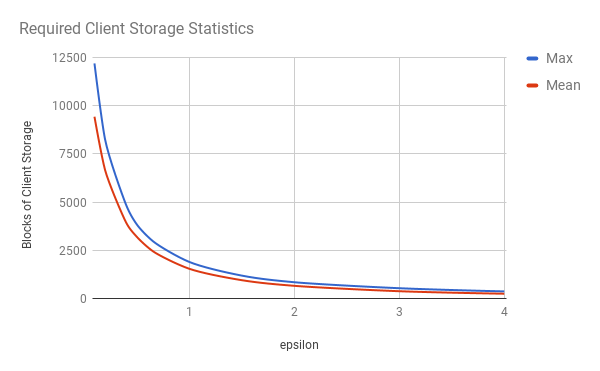
(a) Required client storage for ${\sf CacheShuffle}{\sf Root}$.

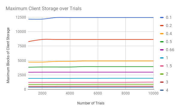
(b) Client storage over trials for ${\sf CacheShuffle}{\sf Root}$.

Figure 2: Client Storage of ${\sf CacheShuffle}{\sf Root}$.

10.1 Client Storage of ${\sf CacheShuffle}{\sf Root}$

We consider multiple instantiations of ${\sf CacheShuffle}{\sf Root}$ with various parameters of $\epsilon$. Each instance is executed over one million blocks of data. From Figure 2a, we see that both the max and mean cache sizes exponentially decrease as $\epsilon$ increases. Also, the max and mean cache sizes do not differ significantly. Furthermore, we run each instance of ${\sf CacheShuffle}{\sf Root}$ on one million blocks over multiple trials and record the max cache size encountered. It turns out the max cache size is reached fairly quickly and does not change as the number of trials increase (see Figure 2b).

10.2 Bandwidth Comparison of ${\sf CacheShuffle}{\sf Root}$ and MelbourneShuffle

In these experiments, we will investigate the hidden constants of ${\sf CacheShuffle}{\sf Root}$ and compare them with the MelbourneShuffle when $K=N$. Asymptotically, both algorithms require $O(\sqrt{N})$ blocks of client storage and $O(N)$ blocks of bandwidth. For practical use cases, the hidden constants are important. For example, the constants affect the costs that cloud service providers must consider for their products. To provide a fair comparison, we will ensure to pick parameters such that CacheShuffle uses the same client storage as the Melbourne Shuffle. The Melbourne Shuffle requires $O(\sqrt{N})$ client storage. Therefore, we can use ${\sf CacheShuffle}_{\sqrt{K},\epsilon}$ since $K=N$ with some small $\epsilon>0$.

Using crude analysis of the hidden constants, we already know that MelbourneShuffle requires $(10+c)N$ blocks of bandwidth and some $c=\Theta(1)$. On the other hand, ${\sf CacheShuffle}{\sf Root}$ uses only $(4+\epsilon)N$ blocks of bandwidth, for small $\epsilon$. In both algorithms, $c$ and $\epsilon$ are directly related with the bandwidth as well as the hidden constants of the required client storage. We attempt to quantify $c$ and $\epsilon$ for practical data sizes and a fixed number of blocks of client storage.

Our experiments run both ${\sf CacheShuffle}{\sf Root}$ and MelbourneShuffle using the same input and output permutations. Furthermore, we assume that exactly $\sqrt{N}$ blocks of client storage are available. It turns out that $\epsilon<1$ is sufficient for ${\sf CacheShuffle}{\sf Root}$, while $c\geq 8$ is required for MelbourneShuffle. Therefore, ${\sf CacheShuffle}{\sf Root}$ is at least a 4x improvement over MelbourneShuffle. A comparison of the performances can be seen in Figure 3.

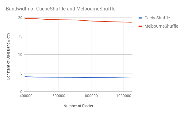
Figure 3: Comparison of ${\sf CacheShuffle}{\sf Root}$ and MelbourneShuffle.

Let us also consider $\sqrt{N}$-Oblivious Shuffling. Again, MelbourneShuffle requires $(10+c)N$ blocks of bandwidth. On the other hand, ${\sf K}{\sf CacheShuffle}{\sf Basic}$ requires exactly $2N$ blocks of bandwidth. So, ${\sf K}{\sf CacheShuffle}{\sf Basic}$ is a 9x improvement for practical sizes of $N$.

10.3 Bandwidth of ${{\sf KCacheShuffleDummy}}$

We investigate the bandwidth costs of ${{\sf KCacheShuffleDummy}}$ in a scenario with dummy blocks. For convenience, we assume that there are $N+D$ input blocks and $N+D$ output blocks. We assume that $D=N$, that is half the blocks are dummies. Using ${\sf K}{\sf CacheShuffle}{\sf Basic}$, we know that $2(N+D)=4N$ blocks of bandwidth are required. On the other hand, ${{\sf KCacheShuffleDummy}}$ only uses $D+(2+\epsilon)N=(3+\epsilon)N$ for some small $\epsilon$. Using experiments, we show that $\epsilon$ is very small for practical data sizes (see Figure 4). Furthermore, as the number of blocks increase, $\epsilon$ decreases.

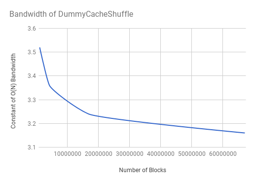
Figure 4: Bandwidth of ${{\sf KCacheShuffleDummy}}$.

Appendix A Revisiting MelbourneShuffle

The notion of Oblivious Shuffling was first introduced in [16], which introduced the Melbourne Shuffle. The Melbourne Shuffle required $O(N)$ blocks of bandwidth and only $O(\sqrt{N})$ client memory. We show that their security notion is an $N$-Oblivious Shuffle.

We recall the original oblivious shuffle security definition. We show that Oblivious Shuffle is exactly $N$-Oblivious Shuffling under the assumption that $\operatorname{\text{\sf Enc}}$ is IND-CPA secure. Specifically, it is assumed in the original Oblivious Shuffling notion that the adversary knows the entirety of $\pi$, the input allocation map.

Definition A.1 (Shuffle-IND).

For challenger ${{\mathcal{C}}}$ with shuffle algorithm ${{\mathsf{Sh}}}$ and adversary ${{\mathcal{A}}}$, we define game ${\mathsf{ShuffleIndGame}}_{{\mathcal{A}}}^{{{\mathsf{Sh}}}}(N,\lambda)$ as follows

1. ${{\mathcal{A}}}$ sends $\{B_{i},\pi_{i},\sigma_{i}\}_{i\in[l]}$ to ${{\mathcal{C}}}$ where $l=\operatorname{\text{poly}}(\lambda)$.

2. ${\mathcal{C}}$ sends $\{\pi_{i}(\operatorname{\text{\sf Enc}}(K,B_{i})),{\mathtt{trans}}_{i}\}_{i\in[l]}$ to ${\mathcal{A}}$ where each ${\mathtt{trans}}_{i}$ is picked according to ${{\mathcal{T}}}^{{{\mathsf{Sh}}}}(\pi_{i},\sigma_{i})$.

3. ${\mathcal{A}}$ submits distinct $(C_{0},\rho_{0},\rho^{\prime}_{0})$ and $(C_{1},\rho_{1},\rho^{\prime}_{1})$ to ${\mathcal{A}}$ as the challenge.

4. ${{\mathcal{C}}}$ random selects $b\leftarrow\{0,1\}$. ${{\mathcal{C}}}$ sends $\{\rho_{b}(\operatorname{\text{\sf Enc}}(K,C_{b})),{\mathtt{trans}}\}$ to ${{\mathcal{A}}}$ where ${\mathtt{trans}}$ is drawn according to ${{\mathcal{T}}}^{{{\mathsf{Sh}}}}(\rho_{b},\rho^{\prime}_{b})$.

5. Repeat Steps 1-2.

6. ${\mathcal{A}}$ outputs $b^{\prime}$.

Output 1 iff $b=b^{\prime}$.

Definition A.2 (Shuffle-IND Secure).

Suppose that ${{\mathsf{Sh}}}$ is a shuffling algorithm over $N=\operatorname{\text{poly}}(k)$ items. Then, ${{\mathsf{Sh}}}$ is Shuffle-IND secure if for every probabilistically polynomial-time bounded adversary ${\mathcal{A}}$

$$\Pr[{\mathsf{ShuffleIndGame}}_{{\mathcal{A}}}^{{{\mathsf{Sh}}}}(N,\lambda)=1]\leq\frac{1}{2}+\operatorname{\text{negl}}(N).$$

Theorem A.1.

${{\mathsf{Sh}}}$ is Shuffle-IND secure if and only if ${{\mathsf{Sh}}}$ is an Oblivious Shuffle.

Proof.

We compare the two games ${\mathsf{ShuffleIndGame}}$ and ${\mathsf{OSGame}}$ with an $N$-restricted adversary. That is, we are allowing ${{\mathcal{A}}}$ to pick the entirety of the input permutations for ${\mathsf{OSGame}}$. If we remove steps 1-2 and 5 from ${\mathsf{ShuffleIndGame}}$, the games are identical. However, we see that ${{\mathcal{A}}}$ can simulate steps 1-2 and 5 without the help of ${\mathcal{C}}$ since ${{\mathsf{Sh}}}$ is known to ${{\mathcal{A}}}$. Therefore, the games are identical. ∎

Appendix B ${\sf CacheShuffle}{\sf Root}$ Pseudocode

${\sf CacheShuffle}{\sf Root}$ 1 Oblivious Shuffling with $O(\sqrt{N})$ client storage.

0:  $\pi,\sigma,{{\mathsf{Source}}},{{\mathsf{Dest}}}$

  Set $\nu\leftarrow\sqrt{K}$ and ${\xi}\leftarrow(1+\epsilon/2)\sqrt{K}$.

  Set ${\mathsf{cnt}}\leftarrow 0$ and ${\mathsf{cnt}}_{\nu}\leftarrow 1$.

  Initialize ${{\mathsf{srcInd}}}_{1},\ldots,{{\mathsf{srcInd}}}_{\nu}$ to be empty on the client.

  for all $i\in{\mathsf{Touched}}$ do

     Set ${{\mathsf{srcInd}}}_{{\mathsf{cnt}}_{\nu}}\leftarrow{{\mathsf{srcInd}}}_{{\mathsf{cnt}}_{\nu}}\cup\{i\}$.

     Increment ${\mathsf{cnt}}$ by 1.

     if ${\mathsf{cnt}}=\sqrt{K}$ then

        Set ${\mathsf{cnt}}\leftarrow 0$.

        Increment ${\mathsf{cnt}}_{\nu}$ by 1.

     end if

  end for

  Initialize ${\mathsf{dMap}}$ to be an empty key-value storage.

  Initialize ${\mathsf{destB}}_{1},\ldots,{\mathsf{destB}}_{{\xi}}$ to be empty on the client.

  for all $i\in[N]$ do

     Choose $j$ uniformly at random from $[{\xi}]$.

     Set ${\mathsf{destB}}_{j}\leftarrow{\mathsf{destB}}_{j}\cup\{i\}$.

     Set ${\mathsf{dMap}}[i]\leftarrow j$.

  end for

  Initialize ${\mathsf{Q}}_{1},\ldots,{\mathsf{Q}}_{{\xi}}$ to be empty maps on the client.

  Initialize ${{\mathsf{temp}}}_{1},\ldots,{{\mathsf{temp}}}_{{\xi}}$ to be empty on the server with $p$ empty slots for blocks each.

  for $i=1,\ldots,\nu$ do

     Run $\text{\sf Spray}(\pi,\sigma,{\mathsf{dMap}},{{\mathsf{Source}}},{{\mathsf{srcInd}}}_{i},{\mathsf{Q}}_{1},\ldots,{\mathsf{Q}}_{{\xi}},{{\mathsf{temp}}}_{1},\ldots,{{\mathsf{temp}}}_{{\xi}})$.

  end for

  for $i=1,\ldots,{\xi}$ do

     Run $\text{\sf Recalibrate}(\pi,\sigma,{{\mathsf{Source}}},{{\mathsf{Dest}}},{\mathsf{destB}}_{i},{\mathsf{Q}}_{i},{{\mathsf{temp}}}_{i})$.

  end for

Spray 2 The Spray phase of ${\sf CacheShuffle}{\sf Root}$.

0:  $\pi,\sigma,{\mathsf{dMap}},{{\mathsf{Source}}},{{\mathsf{srcInd}}},{\mathsf{Q}}_{1},\ldots,{\mathsf{Q}}_{{\xi}},{{\mathsf{temp}}}_{1},\ldots,{{\mathsf{temp}}}_{{\xi}}$

  for all $i\in{{\mathsf{srcInd}}}$ do

     Download ${{\mathsf{Source}}}[\pi(i)]$.

     Set $B_{i}\leftarrow\operatorname{\text{\sf Dec}}({{\mathtt{key}}},{{\mathsf{Source}}}[\pi(i)])$.

     Set ${\mathsf{pos}}_{i}\leftarrow{\mathsf{dMap}}[\sigma(i)]$.

     Set ${\mathsf{Q}}_{{\mathsf{pos}}_{i}}[\sigma(i)]\leftarrow B_{i}$.

  end for

  for $i=1,\ldots,{\xi}$ do

     if ${\mathsf{Q}}_{i}\neq\emptyset$ then

        Remove any element $B$ from ${\mathsf{Q}}_{i}$.

        Upload $\operatorname{\text{\sf Enc}}({{\mathtt{key}}},B)$ to ${{\mathsf{temp}}}_{i}$.

     else

        Upload $\operatorname{\text{\sf Enc}}({{\mathtt{key}}},{\mathbf{0}})$ to ${{\mathsf{temp}}}_{i}$.

     end if

  end for

Recalibrate 3 The Recalibrate phase of ${\sf CacheShuffle}{\sf Root}$.

0:  $\pi,\sigma,{{\mathsf{Source}}},{{\mathsf{Dest}}},{\mathsf{destB}},{\mathsf{Q}},{{\mathsf{temp}}}$

  Download ${{\mathsf{temp}}}$ from the server.

  for all blocks $B\in{{\mathsf{temp}}}$ do

     Set $B\leftarrow\operatorname{\text{\sf Enc}}({{\mathtt{key}}},B)$.

     Set ${\mathsf{Q}}[\sigma(B.{\mathsf{idx}})]\leftarrow B$.

  end for

  for all $j\in{\mathsf{destB}}$ do

     Upload $\operatorname{\text{\sf Enc}}({{\mathtt{key}}},{\mathsf{Q}}[j])$ to ${\mathsf{destB}}[j]$.

     Remove ${\mathsf{Q}}[j]$.

  end for

Appendix C ${\sf K}{\sf CacheShuffle}{\sf Basic}$ Pseudocode

${\sf K}{\sf CacheShuffle}{\sf Basic}$ 4 $K$-Oblivious Shuffle with $O(K)$ client storage.

0:  $\pi,\sigma,{\mathsf{Source}},{\mathsf{Dest}},{\mathsf{Touched}}$

  Initialize ${\mathsf{tbDown}}\leftarrow[N]$.

  Initialize ${\mathbb{U}}$ to be an empty map on the client.

  for all $i\in{\mathsf{Touched}}$ do

     Download $B\leftarrow{\mathsf{Source}}[\pi(i)]$.

     Set ${\mathbb{U}}[i]\leftarrow\operatorname{\text{\sf Dec}}({{\mathtt{key}}},B)$.

     Set ${\mathsf{tbDown}}\leftarrow{\mathsf{tbDown}}\ /\ \{\pi(i)\}$.

  end for

  for $i=1,\ldots,N$ do

     if $i\leq N-K$ then

        if $\sigma^{-1}(i)\notin{\mathsf{tbDown}}$ then

           Pick $j$ uniformly at random from ${\mathsf{tbDown}}$.

           Download $B\leftarrow{\mathsf{Source}}[\pi(j)]$.

           Set ${\mathbb{U}}[j]\leftarrow\operatorname{\text{\sf Dec}}({{\mathtt{key}}},B)$.

           Set ${\mathsf{tbDown}}\leftarrow{\mathsf{tbDown}}\ /\ \{j\}$.

        else

           Download $B\leftarrow{\mathsf{Source}}[\pi(\sigma^{-1}(i))]$.

           Set ${\mathbb{U}}[\sigma^{-1}(i)]\leftarrow\operatorname{\text{\sf Dec}}({{\mathtt{key}}},B)$.

           Set ${\mathsf{tbDown}}\leftarrow{\mathsf{tbDown}}\ /\ \{\sigma^{-1}(i)\}$.

        end if

     end if

     Upload $\operatorname{\text{\sf Enc}}({{\mathtt{key}}},{\mathbb{U}}[\sigma^{-1}(i)])$ to ${\mathsf{Dest}}[i]$.

  end for

Appendix D ${{\sf KCacheShuffleDummy}}$ Pseudocode

${{\sf KCacheShuffleDummy}}$ 5 $K$-Oblivious Shuffle including dummies with $O(K)$ client storage.

0:  $\pi,\sigma,{\mathsf{Source}},{\mathsf{Dest}},{\mathsf{Touched}}$

  Initialize ${\mathsf{tbDown}}\leftarrow[M]$.

  Initialize ${\mathbb{U}}$ to be an empty map on the client.

  for all $i\in{\mathsf{Touched}}$ do

     Download $B\leftarrow{\mathsf{Source}}[\pi(i)]$ to client memory.

     Set ${\mathbb{U}}[i]\leftarrow\operatorname{\text{\sf Dec}}({{\mathtt{key}}},B)$.

     Set ${\mathsf{tbDown}}\leftarrow{\mathsf{tbDown}}\ /\ \{i\}$.

  end for

  Initialize ${\mathsf{destB}}_{1},\ldots,{\mathsf{destB}}_{p}$ to be empty on client memory.

  for $i=1,\ldots,M$ do

     Pick $r$ uniformly at random from $[p]$.

     Set ${\mathsf{destB}}_{r}\leftarrow{\mathsf{destB}}_{r}\cup\{i\}$.

  end for

  for $i=1,\ldots,p$ do

     if $|{\mathsf{destB}}_{i}|>(1+\epsilon)K$ then

        Abort algorithm and fail.

     else if $|\{d\in{\mathsf{destB}}_{i}:\sigma(d)\neq\perp\}|>(1+\epsilon)\rho K$ then

        Abort algorithm and fail.

     end if

     for all $d\in{\mathsf{destB}}_{i}$ do

        if $d\in{\mathsf{tbDown}}$ then

           Download $B\leftarrow{\mathsf{Source}}[\pi(d)]$.

           Set ${\mathbb{U}}[d]\leftarrow\operatorname{\text{\sf Dec}}({{\mathtt{key}}},B)$.

           Set ${\mathsf{tbDown}}\leftarrow{\mathsf{tbDown}}\ /\ \{d\}$.

        else

           if ${\mathsf{tbDown}}\neq\emptyset$ then

              Pick $r$ uniformly at random from ${\mathsf{tbDown}}$.

              Download $B\leftarrow{\mathsf{Source}}[\pi(r)]$.

              Set ${\mathbb{U}}[r]\leftarrow\operatorname{\text{\sf Dec}}({{\mathtt{key}}},B)$.

              Set ${\mathsf{tbDown}}\leftarrow{\mathsf{tbDown}}\ /\ \{r\}$.

           end if

        end if

     end for

     Construct $f(x)$ such that $f(\sigma(d))=\operatorname{\text{\sf Enc}}({{\mathtt{key}}},{\mathbb{U}}[d])$, for all $d\in{\mathsf{destB}}_{i}$.

     Client sends server the coefficients of $f(x)$ and ${\mathsf{destB}}_{i}^{\prime}\leftarrow\sigma({\mathsf{destB}}_{i})$.

     for all $x\in{\mathsf{destB}}_{i}^{\prime}$ do

        Server places $f(x)$ in location ${\mathsf{Dest}}[x]$.

     end for

  end for

References

- [1] M. Ajtai, J. Komlós, and E. Szemerédi. An O(N log N) sorting network. In Proceedings of the Fifteenth Annual ACM Symposium on Theory of Computing, STOC ’83, pages 1–9. ACM, 1983.
- [2] K. E. Batcher. Sorting networks and their applications. In Proceedings of the April 30–May 2, 1968, Spring Joint Computer Conference, AFIPS ’68 (Spring), pages 307–314. ACM, 1968.
- [3] J. Black and P. Rogaway. CBC MACs for Arbitrary-Length Messages: The Three-Key Constructions, pages 197–215. Springer Berlin Heidelberg, Berlin, Heidelberg, 2000.
- [4] D. Dubhashi and D. Ranjan. Balls and bins: A study in negative dependence. Random Struct. Algorithms, 13(2):99–124, Sept. 1998.
- [5] O. Goldreich. Towards a theory of software protection and simulation by oblivious RAMs. In Proceedings of the Nineteenth Annual ACM Symposium on Theory of Computing, STOC ’87, pages 182–194, New York, NY, USA, 1987. ACM.
- [6] O. Goldreich and R. Ostrovsky. Software protection and simulation on oblivious rams. J. ACM, 43(3):431–473, 1996.
- [7] M. T. Goodrich. Randomized shellsort: A simple data-oblivious sorting algorithm. J. ACM, 58(6):27:1–27:26, Dec. 2011.
- [8] M. T. Goodrich. Zig-Zag sort: A simple deterministic data-oblivious sorting algorithm running in o(n log n) time. In Proceedings of the Forty-sixth Annual ACM Symposium on Theory of Computing, STOC ’14, pages 684–693, New York, NY, USA, 2014. ACM.
- [9] M. T. Goodrich, M. Mitzenmacher, O. Ohrimenko, and R. Tamassia. Oblivious RAM simulation with efficient worst-case access overhead. In Proceedings of the 3rd ACM Workshop on Cloud Computing Security Workshop, CCSW ’11, pages 95–100, New York, NY, USA, 2011. ACM.
- [10] M. T. Goodrich, M. Mitzenmacher, O. Ohrimenko, and R. Tamassia. Privacy-preserving group data access via stateless oblivious RAM simulation. In Proceedings of the Twenty-third Annual ACM-SIAM Symposium on Discrete Algorithms, SODA ’12, pages 157–167, 2012.
- [11] V. T. Hoang, B. Morris, and P. Rogaway. An enciphering scheme based on a card shuffle. In R. Safavi-Naini and R. Canetti, editors, CRYPTO 2012, pages 1–13, 2012.
- [12] C. Liu, L. Zhu, M. Wang, and Y.-A. Tan. Search pattern leakage in searchable encryption: Attacks and new construction. Inf. Sci., 265:176–188, May 2014.
- [13] B. Morris and P. Rogaway. Sometimes-recurse shuffle. In P. Q. Nguyen and E. Oswald, editors, EUROCRYPT 2014, pages 311–326, 2014.
- [14] B. Morris, P. Rogaway, and T. Stegers. How to encipher messages on a small domain. In Advances in Cryptology - CRYPTO 2009, 29th Annual International Cryptology Conference, volume 5677 of Lecture Notes in Computer Science, pages 286–302. Springer, 2009.
- [15] M. Naveed, S. Kamara, and C. V. Wright. Inference attacks on property-preserving encrypted databases. In CCS ’15, pages 644–655. ACM, 2015.
- [16] O. Ohrimenko, M. T. Goodrich, R. Tamassia, and E. Upfal. The Melbourne shuffle: Improving oblivious storage in the cloud. In Automata, Languages, and Programming: 41st International Colloquium, ICALP 2014, Copenhagen, Denmark, July 8-11, 2014, Proceedings, Part II, pages 556–567, 2014.
- [17] R. Ostrovsky and V. Shoup. Private information storage (extended abstract). In Proceedings of the Twenty-ninth Annual ACM Symposium on Theory of Computing, STOC ’97, pages 294–303, New York, NY, USA, 1997. ACM.
- [18] S. Patel, G. Persiano, and K. Yeo. Recursive ORAMs with practical constructions. Cryptology ePrint Archive, Report 2017/964, 2017.
- [19] T. Ristenpart and S. Yilek. The Mix-and-Cut shuffle: Small-domain encryption secure against n queries. In R. Canetti and J. A. Garay, editors, CRYPTO 2013, pages 392–409. Springer, 2013.
- [20] P. Sanders, S. Egner, and J. Korst. Fast concurrent access to parallel disks. In Proceedings of the Eleventh Annual ACM-SIAM Symposium on Discrete Algorithms, SODA ’00, pages 849–858, 2000.
- [21] E. Stefanov, E. Shi, and D. Song. Towards practical oblivious RAM. In NDSS 2012, 2011.
- [22] E. Stefanov, M. van Dijk, E. Shi, C. Fletcher, L. Ren, X. Yu, and S. Devadas. Path ORAM: An extremely simple oblivious RAM protocol. In CCS ’13, pages 299–310. ACM, 2013.