Neutrino Mass, Dark Matter and Baryon Asymmetry without Lepton Number Violation

Abstract

We propose a model to explain tiny masses of neutrinos with the lepton number conservation, where neither too heavy particles beyond the TeV-scale nor tiny coupling constants are required. Assignments of conserving lepton numbers to new fields result in an unbroken $Z_{2}$ symmetry that stabilizes the dark matter candidate (the lightest $Z_{2}$-odd particle). In this model, $Z_{2}$-odd particles play an important role to generate the mass of neutrinos. The scalar dark matter in our model can satisfy constraints on the dark matter abundance and those from direct searches. It is also shown that the strong first-order phase transition, which is required for the electroweak baryogenesis, can be realized in our model. In addition, the scalar potential can in principle contain CP-violating phases, which can also be utilized for the baryogenesis. Therefore, three problems in the standard model, namely absence of neutrino masses, the dark matter candidate, and the mechanism to generate baryon asymmetry of the Universe, may be simultaneously resolved at the TeV-scale. Phenomenology of this model is also discussed briefly.

I Introduction

The standard model (SM) of particle physics was established by the discovery of a Higgs boson at the CERN large hadron collider (LHC) ref:2012Jul . This does not mean that theoretical particle physics has been completed because several problems remain in the high energy physics. For example, neutrinos are massless in the SM while the discovery of neutrino oscillations ref:numass is the evidence of tiny neutrino masses. The absence of the candidate for the dark matter in the SM, which accounts for 27% of the Universe Ade:2015xua , must be resolved. The baryon asymmetry of the Universe cannot be explained in the SM, so that the SM must be extended to include a mechanism to generate the baryon asymmetry of the Universe.

Reasons why neutrinos are massless in the SM are the absence of right-handed neutrinos $\nu_{R}$ and the lepton number conservation. If we introduce $\nu_{R}$ to the SM, neutrino masses can be generated via the naive Yukawa interaction with the Higgs doublet field in the SM similarly to masses of quarks and charged leptons. However, the Yukawa coupling constant seems to be unnaturally small ($\lesssim 10^{-12}$). Instead of such fine-tuned coupling constants, in the (type-I) seesaw mechanism ref:seesaw very large Majorana masses of $\nu_{R}$ are introduced with the lepton number violation for a natural realization of tiny neutrino masses. Such heavy Majorana neutrinos can also be used for leptogenesis Fukugita:1986hr to explain the baryon asymmetry of the Universe.

There is an alternative scenario, in which the smallness of neutrino masses can be explained by the quantum effect. For example, tiny Majorana masses are radiatively generated at the one-loop level in the Ma model ref:Ma , where new particles are not necessarily very heavy and can be in the TeV-scale. Hence, scenarios along this line can be in principle tested directly by collider experiments. In addition, new particles that are involved in the one-loop diagram include the dark matter candidate. Similarly to the Ma model, the Aoki-Kanemura-Seto (AKS) model ref:AKS gives tiny Majorana neutrino masses at the three-loop level, where the dark matter candidate contributes to the three-loop diagram. One of the remarkable features of this model is that two ${\text{SU}}(2)_{L}$-doublet Higgs fields are required. In general two Higgs doublet models can contain CP violating phases in the Higgs sector. It is shown that the strong first-order phase transition is realized in the AKS model which is required for successful electroweak baryogenesis Kuzmin:1985mm . Thus, three problems can be simultaneously resolved at the TeV-scale in the AKS model, which can be probed at collider experiments.

In Refs. Kanemura:2015cca ; Kanemura:2016ixx , models for generating the neutrino mass matrix are classified into several groups by focusing on combinations of Yukawa matrices in the mass matrix. In the systematic study for the Majorana neutrino mass generation Kanemura:2015cca , no combination other than the one in the AKS model involves simultaneously the dark matter candidate and the second ${\text{SU}}(2)_{L}$-doublet Higgs field that has the vacuum expectation value. On the other hand, it was found in Ref. Kanemura:2016ixx that masses of Dirac neutrinos can be radiatively generated by using the dark matter candidate and the second ${\text{SU}}(2)_{L}$-doublet Higgs field (See Figs. 11, 13 and 15 in Ref. Kanemura:2016ixx ).

In this letter, we propose a concrete model, where the combination of Yukawa matrices to generate Dirac neutrino mass matrix corresponds to the structure in Fig. 15 in Ref. Kanemura:2016ixx . As the lepton number violating phenomena such as the neutrinoless double beta decay have not been observed up to now, it would be important to consider the possibility that neutrinos are purely of the Dirac type fermions, whose masses conserve the lepton number. Along this line, we investigate the new model to simultaneously provide the origin of tiny neutrino masses, the dark matter candidate, and the source of the baryon asymmetry of the Universe. We here ignore the CP violation in the scalar potential for simplicity and concentrate on the realization of the strong first-order phase transition, which is necessary for successful electroweak baryogenesis. Calculation for the baryon asymmetry with the CP violation is beyond the scope of this letter, and leave it as our future work.

This letter is organized as follows. In Sec. II, we present our model where Dirac neutrino masses are generated at the one-loop level. We see that our model can be consistent with neutrino oscillation data and the relic abundance of the dark matter as well as the strong first-order electroweak phase transition required for the electroweak baryogenesis scenario. Section III is devoted to further phenomenological studies such as lepton flavor violating decays of charged leptons, the spin-independent scattering cross section of the dark matter on a proton, and collider phenomenology. Conclusions are shown in Sec. IV. Some formulae are presented in Appendix.

II The Model

	$Z_{2}$-even					$Z_{2}$-odd
	$\ell_{R}$	$\nu_{R}$	$\Phi_{1}$	$\Phi_{2}$	$s_{3}^{+}$	$\psi_{R}^{0}$	$s_{2}^{0}$	$s_{2}^{+}$
Spin	$1/2$	$1/2$	$0$	$0$	$0$	$1/2$	$0$	$0$
${\text{SU}}(2)_{L}$	$\bf\underline{1}$	$\bf\underline{1}$	$\bf\underline{2}$	$\bf\underline{2}$	$\bf\underline{1}$	$\bf\underline{1}$	$\bf\underline{1}$	$\bf\underline{1}$
${\text{U}}(1)_{Y}$	$-1$	$0$	$1/2$	$1/2$	$1$	$0$	$0$	$1$
Lepton Number	$1$	$1$	$0$	$0$	$0$	$0$	$-1$	$-1$
$Z_{2}^{\prime}$	Even	Odd	Even	Even		Even	Odd	Even
$Z_{2}^{\prime\prime}$	Odd	Even	Odd	Even	Odd	Even	Even	Odd

Table 1: The list of new fields in our model, which are added to the SM. A scalar field $s_{3}^{+}$ can be both of even and odd for the $Z_{2}^{\prime}$ symmetry.

II.1 Particle contents and Lagrangian

In our model, the lepton number (L) conservation is imposed. We introduce gauge singlet fermions $\nu_{iR}$ ($i=1\text{--}3$) with $L=1$, which result in right-handed components of Dirac neutrinos. New fields that are introduced to the SM are listed in Table 1. Fermions $\psi_{aR}^{0}$ ($a=1\text{--}3$) are also gauge singlet though they have $L=0$ in comparison with $L=1$ for $\nu_{R}$. This model involves two ${\text{SU}}(2)_{L}$-doublet scalar fields $\Phi_{1}\equiv(\phi_{1}^{+},(v_{1}+\phi_{1r}^{0}+i\phi_{1i}^{0})/\sqrt{2})^{T}$ and $\Phi_{2}\equiv(\phi_{2}^{+},(v_{2}+\phi_{2r}^{0}+i\phi_{2i}^{0})/\sqrt{2})^{T}$ with $Y=1/2$ and $L=0$, where $v^{2}=v_{1}^{2}+v_{2}^{2}=(246\,{\text{GeV}})^{2}$. Scalar fields $s_{2}^{+}$ and $s_{3}^{+}$ are ${\text{SU}}(2)_{L}$-singlet with $Y=1$; the former has $L=-1$ while the latter does $L=0$. The complex scalar field $s_{2}^{0}$ is a gauge singlet with $L=-1$.

If the Dirac neutrino mass is simply generated via the Yukawa interaction $y_{\nu}\overline{L}\widetilde{\Phi}\nu_{R}$, where $\widetilde{\Phi}\equiv\epsilon\Phi^{\ast}$, the size of the Yukawa coupling constant is extremely small ($y_{\nu}\sim 10^{-12}$), which seems to be unnatural and cannot be experimentally tested. In our model, the Yukawa interaction is forbidden at the tree-level by imposing a softly broken $Z_{2}$ symmetry (we refer to it as the $Z_{2}^{\prime}$ symmetry), under which $\nu_{R}$ is odd while ${\text{SU}}(2)_{L}$-doublet lepton and scalars are even. Properties of additional particles with respect to the $Z_{2}^{\prime}$ are also shown in Table 1. The scalar field $s_{3}^{+}$ can be both of even and odd. The $Z_{2}^{\prime}$ is softly broken in the scalar potential, and then the Dirac neutrino mass can be generated at the two-loop level as we see later.

Relevant parts of Yukawa interactions for generating neutrino masses are given by

$${\mathcal{L}}_{\text{Yukawa}}=y_{\ell}\overline{L_{\ell}}\Phi_{1}\ell_{R}+(Y_{\psi}^{+})_{\ell a}\overline{(\ell_{R})^{c}}\,{\color[rgb]{1,0,0}\psi_{aR}^{0}\,s_{2}^{+}}+(Y_{\psi}^{0})_{ia}\overline{(\nu_{iR})^{c}}\,{\color[rgb]{1,0,0}\psi_{aR}^{0}\,s_{2}^{0}}+\text{h.c.}$$ (1)

In order to forbid the flavor changing neutral current (FCNC) at the tree level, we impose another softly-broken $Z_{2}$ symmetry (we represent it as $Z_{2}^{\prime\prime}$) as shown in Table. 1. Quarks and the lepton doublet field are $Z_{2}^{\prime\prime}$-even. Then, $\ell_{R}$ has the Yukawa interaction only with $\Phi_{1}$ similarly to the the type-X two Higgs doublet model Aoki:2009ha (see also Refs. Barger:1989fj ; Grossman:1994jb ; ref:THDM-Akeroyd ).

The scalar potential is given by

$$V = V_{\text{THDM}}+m_{s0}^{2}|{\color[rgb]{1,0,0}s_{2}^{0}}|^{2}+m_{s2}^{2}|{\color[rgb]{1,0,0}s_{2}^{+}}|^{2}+m_{s3}^{2}|s_{3}^{+}|^{2}$$ (2)

$${}+\left(\mu_{3}\Bigl{[}\Phi_{2}^{\dagger}\epsilon\Phi_{1}^{\ast}s_{3}^{+}\Bigr{]}+\text{h.c.}\right)+\left(\mu_{3}^{\prime}\Bigl{[}s_{3}^{-}{\color[rgb]{1,0,0}s_{2}^{+}s_{2}^{0\ast}}\Bigr{]}+\text{h.c.}\right)$$

$${}+\lambda_{s0s2}|{\color[rgb]{1,0,0}s_{2}^{0}}|^{2}|{\color[rgb]{1,0,0}s_{2}^{+}}|^{2}+\lambda_{s0s3}|{\color[rgb]{1,0,0}s_{2}^{0}}|^{2}|s_{3}^{+}|^{2}+\lambda_{s2s3}|{\color[rgb]{1,0,0}s_{2}^{+}}|^{2}|s_{3}^{+}|^{2}$$

$${}+\lambda_{\phi 1s0}\Phi_{1}^{\dagger}\Phi_{1}|{\color[rgb]{1,0,0}s_{2}^{0}}|^{2}+\lambda_{\phi 1s2}\Phi_{1}^{\dagger}\Phi_{1}|{\color[rgb]{1,0,0}s_{2}^{+}}|^{2}+\lambda_{\phi 1s3}\Phi_{1}^{\dagger}\Phi_{1}|s_{3}^{+}|^{2}$$

$${}+\lambda_{\phi 2s0}\Phi_{2}^{\dagger}\Phi_{2}|{\color[rgb]{1,0,0}s_{2}^{0}}|^{2}+\lambda_{\phi 2s2}\Phi_{2}^{\dagger}\Phi_{2}|{\color[rgb]{1,0,0}s_{2}^{+}}|^{2}+\lambda_{\phi 2s3}\Phi_{2}^{\dagger}\Phi_{2}|s_{3}^{+}|^{2}$$

$${}+\lambda_{s0}|{\color[rgb]{1,0,0}s_{2}^{0}}|^{4}+\lambda_{s2}|{\color[rgb]{1,0,0}s_{2}^{+}}|^{4}+\lambda_{s3}|s_{3}^{+}|^{4},$$

where $V_{\text{THDM}}$ is the following one in two Higgs double models without the tree-level FCNC:

$$V_{\text{THDM}} = m_{11}^{2}\Phi_{1}^{\dagger}\Phi_{1}+m_{22}^{2}\Phi_{2}^{\dagger}\Phi_{2}-\left(m_{12}^{2}\Phi_{1}^{\dagger}\Phi_{2}+\text{h.c.}\right)$$ (3)

$${}+\frac{\lambda_{1}}{2}(\Phi_{1}^{\dagger}\Phi_{1})^{2}+\frac{\lambda_{2}}{2}(\Phi_{2}^{\dagger}\Phi_{2})^{2}+\lambda_{3}(\Phi_{1}^{\dagger}\Phi_{1})(\Phi_{2}^{\dagger}\Phi_{2})$$

$${}+\lambda_{4}(\Phi_{1}^{\dagger}\Phi_{2})(\Phi_{2}^{\dagger}\Phi_{1})+\left(\frac{\lambda_{5}}{2}(\Phi_{1}^{\dagger}\Phi_{2})^{2}+\text{h.c.}\right).$$

The complex phases of $\mu_{3}$, $\mu_{3}^{\prime}$, and $\lambda_{5}$ can be eliminated by the rephasing of $s_{3}^{+}$, $s_{2}^{+}$ (or $s^{0}$), and $\Phi_{1}$ (or $\Phi_{2}$), respectively. For simplicity in this letter, we take $m_{12}^{2}$ as a real parameter and also assume that the CP is not spontaneously violated. $Z_{2}^{\prime}$ and $Z_{2}^{\prime\prime}$ symmetries are softly broken by $\mu_{3}\mu_{3}^{\prime}$ and $m_{12}^{2}$, respectively.

By virtue of the assignments of conserved lepton numbers to new fields, there appears an unbroken $Z_{2}$ symmetry such that $\psi_{R}^{0}$, $s_{2}^{0}$, and $s_{2}^{+}$ have the odd parity. The $Z_{2}$ symmetry can be utilized for the stabilization of the dark matter candidate.

$Z_{2}$-odd scalar fields $s_{2}^{0}$ and $s_{2}^{+}$ are mass eigenstates ${\mathcal{H}}^{0}$ and ${\mathcal{H}}^{+}$ without mixings with other fields, respectively. Their masses are calculated as

$$m_{{\mathcal{H}}^{0}}^{2} = m_{s0}^{2}+\frac{\lambda_{\phi 1s0}v_{1}^{2}}{2}+\frac{\lambda_{\phi 2s0}v_{2}^{2}}{2},$$ (4)

$$m_{{\mathcal{H}}^{+}}^{2} = m_{s2}^{2}+\frac{\lambda_{\phi 1s2}v_{1}^{2}}{2}+\frac{\lambda_{\phi 2s2}v_{2}^{2}}{2}.$$ (5)

Three $Z_{2}$-even charged scalar fields ($\phi_{1}^{+}$, $\phi_{2}^{+}$, and $s_{3}^{+}$) result in three mass eigenstates ($H_{1}^{+}$, $H_{2}^{+}$, and the Nambu-Goldstone boson $G^{+}$) as

$$\begin{pmatrix}G^{+}\\ H_{1}^{+}\\ H_{2}^{+}\end{pmatrix}=\begin{pmatrix}\cos\beta&\sin\beta&0\\ -\sin\beta\cos\theta_{+}&\cos\beta\cos\theta_{+}&\sin\theta_{+}\\ \sin\beta\sin\theta_{+}&-\cos\beta\sin\theta_{+}&\cos\theta_{+}\end{pmatrix}\begin{pmatrix}\phi_{1}^{+}\\ \phi_{2}^{+}\\ s_{3}^{+}\end{pmatrix},$$ (6)

where $\tan\beta=v_{2}/v_{1}$. The mixing angle $\theta_{+}$ can be expressed as

$$\tan(2\theta_{+}) = \frac{-2(M_{H^{+}}^{\prime 2})_{12}}{(M_{H^{+}}^{\prime 2})_{22}-(M_{H^{+}}^{\prime 2})_{11}},$$ (7)

where the $2\times 2$ matrix $M_{H^{+}}^{\prime 2}$ is defined as

$$M_{H^{+}}^{\prime 2}\equiv\begin{pmatrix}\displaystyle\frac{v^{2}}{v_{1}v_{2}}m_{12}^{2}-\frac{1}{\,2\,}(\lambda_{4}+\lambda_{5})v^{2}&\displaystyle\frac{v\mu_{3}}{\sqrt{2}}\\ \displaystyle\frac{v\mu_{3}}{\sqrt{2}}&\displaystyle m_{s3}^{2}+\frac{\lambda_{\phi 1s3}v_{1}^{2}}{2}+\frac{\lambda_{\phi 2s3}v_{2}^{2}}{2}\end{pmatrix}.$$ (8)

Masses of $H_{1}^{+}$ and $H_{2}^{+}$ are given by

$$m_{H_{1}^{+}}^{2} = \frac{1}{\,2\,}\left\{(M_{H^{+}}^{\prime 2})_{11}+(M_{H^{+}}^{\prime 2})_{22}-\sqrt{((M_{H^{+}}^{\prime 2})_{22}-(M_{H^{+}}^{\prime 2})_{11})^{2}+4(M_{H^{+}}^{\prime 2})_{12}^{2}}\right\},$$ (9)

$$m_{H_{2}^{+}}^{2} = \frac{1}{\,2\,}\left\{(M_{H^{+}}^{\prime 2})_{11}+(M_{H^{+}}^{\prime 2})_{22}+\sqrt{((M_{H^{+}}^{\prime 2})_{22}-(M_{H^{+}}^{\prime 2})_{11})^{2}+4(M_{H^{+}}^{\prime 2})_{12}^{2}}\right\}.$$ (10)

$Z_{2}$-even neutral scalars (CP-even $h$ and $H$, CP-odd $A$, and the Nambu-Goldstone boson $G^{0}$) are constructed from $\Phi_{1}$ and $\Phi_{2}$ similarly to two Higgs doublet models, where $h$ is the discovered Higgs boson with the mass $m_{h}=125\,{\text{GeV}}$. Throughout this letter, we take $\sin(\beta-\alpha)=1$, where $\alpha$ denotes the mixing angle between $\phi_{1r}^{0}$ and $\phi_{2r}^{0}$.

Differences of our model from the AKS model are as follows.

i) Neutrinos are Dirac fermions, for which right-handed neutrinos $\nu_{R}$ are introduced with the lepton number conservation, while the AKS model is for Majorana neutrino masses without $\nu_{R}$.

ii) Assignments of conserving lepton numbers to new fields stabilize the dark matter candidate instead of the imposed $Z_{2}$ symmetry in the AKS model.

iii) The $Z_{2}$-odd neutral scalar $s_{2}^{0}$ is a complex field with the conserved lepton number while the AKS model involves a $Z_{2}$-odd real scalar field.

iv) The $Z_{2}$-even ${\text{SU}}(2)_{L}$-singlet charged scalar $s_{3}^{+}$ is introduced, which is absent in the AKS model.

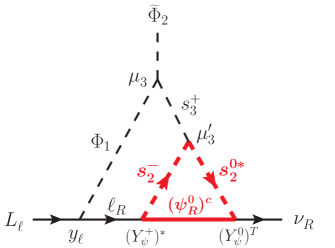
Figure 1: The diagram for generating Dirac neutrino masses in our model. The arrow shows the flow of the lepton number, which is conserved in our model.

II.2 Dirac Neutrino Masses

Neutrinos acquire Dirac masses at the two-loop level as $(m_{\text{D}})_{\ell i}\,\overline{\nu_{\ell L}}\,\nu_{iR}$ via the diagram in Fig. 1. Notice that the interaction $\Phi_{2}^{\dagger}\epsilon\Phi_{1}^{\ast}s_{2}^{+}s_{2}^{0}$ is forbidden because this is a hard breaking term of $Z_{2}^{\prime}$. The coupling constant $\mu_{3}$ can be expressed by $\theta_{+}$. Although arbitrary number of $|\Phi_{i}|^{2}$ can be attached to each of scalar lines in the diagram with appropriate coupling constant $\lambda$, such effects to neutrino masses are involved in scalar mass eigenvalues as $\lambda v_{i}^{2}$. As a result, the mass matrix $(m_{\text{D}})_{\ell i}$ is given by

$$(m_{\text{D}})_{\ell i} = \frac{1}{\sqrt{2}\,v}\,m_{\ell}\left(m_{H_{2}^{+}}^{2}-m_{H_{1}^{+}}^{2}\right)\mu_{3}^{\prime}\tan\beta\,\sin(2\theta_{+})\sum_{a}(Y_{\psi}^{+})^{\ast}_{\ell a}(Y_{\psi}^{0})^{T}_{ai}I_{\ell a},$$ (11)

where the explicit formula for the two-loop function $I_{\ell a}$ is presented in Appendix A. We can take the basis where $\nu_{iR}$ are already mass eigenstates without loss of generality. Then, the mass matrix can be expressed as $m_{\text{D}}=U_{\text{MNS}}\,\text{diag}(m_{1},m_{2},m_{3})$ with neutrino mass eigenvalues $m_{i}$ ($i=1\text{-}3$). The Maki-Nakagawa-Sakata matrix Maki:1962mu $U_{\text{MNS}}$ can be parametrized as

$$U_{\text{MNS}}=\begin{pmatrix}1&0&0\\ 0&c_{23}&s_{23}\\ 0&-s_{23}&c_{23}\end{pmatrix}\begin{pmatrix}c_{13}&0&s_{13}e^{-i\delta}\\ 0&1&0\\ -s_{13}e^{i\delta}&0&c_{13}\end{pmatrix}\begin{pmatrix}c_{12}&s_{12}&0\\ -s_{12}&c_{12}&0\\ 0&0&1\end{pmatrix},$$ (12)

where $c_{ij}\equiv\cos\theta_{ij}$ and $s_{ij}\equiv\sin\theta_{ij}$. Neutrino oscillation data result in We take the following values consistent with neutrino oscillation data:

$$\sin^{2}\theta_{23}=0.514~{}\text{\cite[cite]{\@@bibref{Authors Phrase1YearPhrase2}{Abe:2015awa}{\@@citephrase{(}}{\@@citephrase{)}}}},\quad\sin^{2}(2\theta_{13})=0.0841~{}\text{\cite[cite]{\@@bibref{Authors Phrase1YearPhrase2}{An:2016ses}{\@@citephrase{(}}{\@@citephrase{)}}}},\quad\tan^{2}\theta_{12}=0.427~{}\text{\cite[cite]{\@@bibref{Authors Phrase1YearPhrase2}{Aharmim:2011vm}{\@@citephrase{(}}{\@@citephrase{)}}}},$$ (13)

$$\Delta m^{2}_{32}=2.51\times 10^{-3}\,{\text{eV}}^{2}~{}\text{\cite[cite]{\@@bibref{Authors Phrase1YearPhrase2}{Abe:2015awa}{\@@citephrase{(}}{\@@citephrase{)}}}},\quad\Delta m^{2}_{21}=7.46\times 10^{-5}\,{\text{eV}}^{2}~{}\text{\cite[cite]{\@@bibref{Authors Phrase1YearPhrase2}{Aharmim:2011vm}{\@@citephrase{(}}{\@@citephrase{)}}}},$$ (14)

where $\Delta m^{2}_{ij}\equiv m_{i}^{2}-m_{j}^{2}$. For example, $m_{\text{D}}$ for these values with $m_{3}>m_{1}=0.01\,{\text{eV}}$ and $\delta=0$ can be generated in our model by the following benchmark set of parameter values:

$$\begin{split}&Y_{\psi}^{+}=\begin{pmatrix}1&0.01&0.01\\ 0.01&1&0.01\\ 0.01&0.01&1\end{pmatrix},\quad Y_{\psi}^{0}\simeq\begin{pmatrix}3.2\times 10^{-1}&-4.0\times 10^{-3}&-3.1\times 10^{-3}\\ 2.7\times 10^{-1}&-1.4\times 10^{-3}&-2.8\times 10^{-3}\\ 2.9\times 10^{-1}&3.9\times 10^{-3}&-2.6\times 10^{-3}\end{pmatrix},\\ &\mu_{3}^{\prime}=50\,{\text{GeV}},\quad\tan\beta=3,\quad\sin\theta_{+}=0.1,\\ &m_{H_{1}^{+}}=200\,{\text{GeV}},\quad m_{H_{2}^{+}}=300\,{\text{GeV}},\quad m_{{\mathcal{H}}^{+}}=350\,{\text{GeV}},\quad m_{{\mathcal{H}}^{0}}=63\,{\text{GeV}},\\ &m_{\psi_{1R}}=m_{\psi_{2R}}=m_{\psi_{3R}}=5\,{\text{TeV}}.\end{split}$$ (15)

We see that tiny Dirac neutrino masses are obtained without extremely small values of parameters and very heavy particles. Notice that ${\mathcal{H}}^{0}$ for the benchmark set is the lightest $Z_{2}$-odd particle and the dark matter candidate.

For different values of parameters, one of $\psi_{iR}^{0}$ can be the lightest $Z_{2}$-odd particle and the dark matter candidate.

II.3 Relic Abundance of the Dark Matter

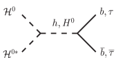
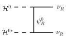
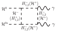
(a)

(b)

(c)

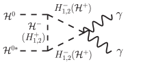
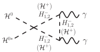
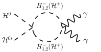
(d)

(e)

(f)

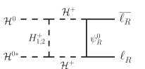
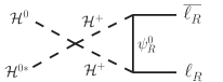
(g)

(h)

Figure 2: Diagrams of the pair-annihilation of ${\mathcal{H}}^{0}$.

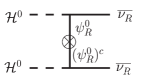
Figure 3: The diagram of the self-annihilation of ${\mathcal{H}}^{0}$.

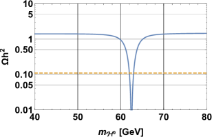
Figure 4: The relic abundance of the scalar dark matter ${\mathcal{H}}^{0}$ in our model. The horizontal dashed line corresponds to $\Omega h^{2}=0.1186$ Ade:2015xua .

For the benchmark set in eq. (15), the dark matter candidate (the lightest $Z_{2}$-odd particle) is a complex scalar particle ${\mathcal{H}}^{0}$. Its relic abundance ($\Omega_{{\mathcal{H}}^{0}}h^{2}+\Omega_{{\mathcal{H}}^{0\ast}}h^{2}\simeq 2\Omega_{{\mathcal{H}}^{0}}h^{2}$) must be consistent with the experimental constraint $\Omega_{\text{DM}}h^{2}=0.1186\pm 0.0020$ Ade:2015xua . Figures 2 and 3 show diagrams of pair and self-annihilation of ${\mathcal{H}}^{0}$, respectively. See Appendix B for formulae of cross sections for them. The cross section $\sigma$, which is the sum of cross sections for these annihilation processes, can be expanded as $\sigma v_{\text{rel}}\simeq\sigma_{0}+\sigma_{1}v_{\text{rel}}^{2}$ with respect to the relative velocity $v_{\text{rel}}$ between initial particles. Then, the relic abundance of ${{\mathcal{H}}^{0}}$ can be calculated Kolb:1990vq with

$$\Omega_{{\mathcal{H}}^{0}}h^{2} = 1.04\times 10^{9}\frac{\sqrt{g_{\ast}}}{g_{\ast S}}\frac{{\text{GeV}}}{m_{\text{Pl}}}\frac{{\text{GeV}}^{-2}}{\sigma_{0}}x_{f}\left(1+\frac{3\sigma_{1}}{\sigma_{0}}x_{f}^{-1}\right)^{-1},$$ (16)

$$x_{f} = \ln\Bigl{[}0.038\,\frac{g_{{\mathcal{H}}^{0}}}{\sqrt{g_{\ast}}}\,m_{\text{Pl}}\,m_{{\mathcal{H}}^{0}}\,\sigma_{0}\Bigr{]}-\frac{1}{\,2\,}\ln\Bigl{[}\Bigl{\{}0.038\,\frac{g_{{\mathcal{H}}^{0}}}{\sqrt{g_{\ast}}}\,m_{\text{Pl}}\,m_{{\mathcal{H}}^{0}}\,\sigma_{0}\Bigr{\}}\Bigr{]}$$ (17)

$$\hskip 85.35826pt{}+\ln\Bigl{[}1+\frac{6\sigma_{1}}{\sigma_{0}}\Bigl{\{}\ln\Bigl{(}0.038\,\frac{g_{{\mathcal{H}}^{0}}}{\sqrt{g_{\ast}}}\,m_{\text{Pl}}\,m_{{\mathcal{H}}^{0}}\,\sigma_{0}\Bigr{)}\Bigr{\}}^{-1}\Bigr{]},$$

where $m_{\text{Pl}}=1.2\times 10^{19}\,{\text{GeV}}$ is the Planck mass, $g_{\ast}=g_{S\ast}=106.75$, and $g_{{\mathcal{H}}^{0}}=1$. Figure 4 is obtained by using the benchmark set in eq. (15) ($m_{{\mathcal{H}}^{0}}$ is taken as the $x$-axis) with

$$m_{H}=200\,{\text{GeV}},\quad\lambda_{\phi 1s0}=0.02,\quad\lambda_{\phi 2s0}=0.005.$$ (18)

We see that the observed value of $\Omega_{\text{DM}}h^{2}$ (horizontal dashed line in Fig. 4) is produced for $m_{{\mathcal{H}}^{0}}=63\,{\text{GeV}}$ of the benchmark set in eq. (15). Since $m_{{\mathcal{H}}^{0}}\simeq m_{h}/2$ for the benchmark set, the $h$-mediation is the dominant annihilation process. Notice that the cross section for the self-annihilation in Fig. 3 is almost independent of $m_{{\mathcal{H}}^{0}}$ if $m_{{\mathcal{H}}^{0}}^{2}\ll m_{\psi}^{2}$. Thus, even for a different value of $m_{{\mathcal{H}}^{0}}$, the constraint on $\Omega_{\text{DM}}h^{2}$ can be easily satisfied by adjusting the overall scale of $Y_{\psi}^{0}$, which does not affect $\ell\to\ell^{\prime}\gamma$ and $\mu\to\overline{e}ee$; the neutrino mass scale can be recovered to the appropriate value by changing $\mu^{\prime}$ for example.

II.4 Strong First-Order Phase Transition

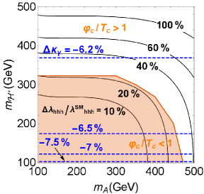
Figure 5: In the white region, our model satisfies the condition $\varphi_{c}/T_{c}\gtrsim 1$ for the strong first-order phase transition, which is required for the electroweak baryogenesis scenario. Solid lines are contours of the deviation $\Delta\lambda_{hhh}/\lambda_{hhh}^{\text{SM}}$ of $\lambda_{hhh}$ from the SM value $\lambda_{hhh}^{\text{SM}}$. Dashed lines show contours of the deviation $\Delta\kappa_{\gamma}$ of $\Gamma(h\to\gamma\gamma)$ from the SM value.

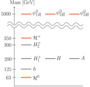
Figure 6: Mass spectrum of $h$ and new particles for the benchmark values in eqs. (15) and (18) with $m_{A}=200\,{\text{GeV}}$. Red bold bars show masses of $Z_{2}$-odd particles.

Baryon asymmetry of the Universe can be generated if the electroweak symmetry is broken via the strong first-order phase transion. Let us examine below whether the strong first-order phase transion can be achieved in our model or not. The effective potential $V_{\text{eff}}$ at the one-loop level at the finite temperature $T$ is given by the sum of the potential $V_{\text{tree}}$ at the tree level, the one-loop correction $\Delta V$ at the zero temperature DiLuzio:2014bua , the correction $\Delta V_{T}$ at the finite temperature Dolan:1973qd as follows:

$$V_{\text{eff}}(\varphi,T) = V_{\text{tree}}(\varphi)+\Delta V(\varphi)+\Delta V_{T}(\varphi,T)+\Delta V_{\text{ring}},$$ (19)

$$V_{\text{tree}}(\varphi) = -\frac{m_{h}^{2}}{4}\varphi^{2}+\frac{m_{h}^{2}}{8v^{2}}\varphi^{4}+\frac{1}{\,2\,}A\varphi^{2},$$ (20)

$$\Delta V(\varphi) = \frac{1}{64\pi^{2}}\sum_{i}n_{i}(-1)^{2s_{i}}\widetilde{m}_{i}^{4}(\varphi)\left(\ln\frac{\widetilde{m}_{i}^{2}(\varphi)}{Q^{2}}-c_{i}\right),$$ (21)

$$\Delta V_{T}(\varphi,T) = \frac{T^{4}}{2\pi^{2}}\sum_{i}n_{i}I_{i}\!\left(\frac{\widetilde{m}_{i}^{2}(\varphi)}{T^{2}}\right),$$ (22)

where $\varphi$ is the order parameter for the electroweak symmetry breaking, $n_{i}$ denotes the degree of freedom for the particle $i$ ($=t,W^{\pm},Z,\gamma$, and scalar bosons), $s_{i}$ is the spin. The field-dependent masses $\widetilde{m}_{i}(\varphi)$ are shown in Appendix C. Contributions from the ring diagrams Carrington:1991hz are taken into account by replacing $\widetilde{m}_{i}(\varphi)$ with $\widetilde{m}_{i}(\varphi,T)$ at a finite temperature $T$, which are given in Appendix D. The constant $c_{i}$ is $3/2$ for fermions and scalar bosons while it is $5/6$ for gauge bosons. The counter term $A$ and the renormalization scale $Q$ can be determined by renormalization conditions $\partial V_{\text{eff}}(\varphi,0)/\partial\varphi|_{\varphi=v}=0$ and $\partial^{2}V_{\text{eff}}(\varphi,0)/\partial\varphi^{2}|_{\varphi=v}=m_{h}^{2}$, where the infrared diverging $\ln\widetilde{m}_{i}^{2}(v)$ of the Nambu-Goldstone bosons ($i=G^{0},G^{\pm}$) are replaced with $\text{Re}\int_{0}^{1}dx\ln\{-x(1-x)m_{h}^{2}\}$ Cline:1996mga . The distribution functions are given by $I_{i}(\alpha^{2})=\int_{0}^{\infty}\!\!dx\,x^{2}\ln\{1\mp\exp(-\sqrt{x^{2}+\alpha^{2}})\}$, where the minus sign is for bosons and the plus sign is for fermions Dolan:1973qd . The critical temperature $T_{c}$ and the critical value $\varphi_{c}$ ($\varphi$ at $T_{c}$) are obtained with $V_{\text{eff}}(\varphi_{c},T_{c})=0$ and $\partial V_{\text{eff}}(\varphi,T_{c})/\partial\varphi|_{\varphi=\varphi_{c}}=0$. Then, $\varphi_{c}/T_{c}\gtrsim 1$ is required for the strong first-order phase transition Kuzmin:1985mm . It is shown in Fig. 5 that the condition is satisfied in the white region ($m_{A}\gtrsim 470\,{\text{GeV}}$ and $m_{{\mathcal{H}}^{\pm}}\gtrsim 300\,{\text{GeV}}$). By taking $m_{A}=200\,{\text{GeV}}$ as a benchmark value together with values in eqs. (15) and (18), the mass spectrum of scalar bosons and $\psi_{R}^{0}$ are presented in Fig. 6.

III Phenomenology

The Yukawa interaction with $Y_{\psi}^{+}$ causes $\ell\to\ell^{\prime}\gamma$ via the ${\mathcal{H}}^{+}$-$\psi_{R}^{0}$ loop. The branching ratio is calculated as

$$\text{BR}(\ell\to\ell^{\prime}\gamma)=\frac{3\alpha_{\text{EM}}}{64\pi G_{F}^{2}m_{{\mathcal{H}}^{+}}^{4}}\Bigl{|}(Y_{\psi}^{+}(Y_{\psi}^{+})^{\dagger})_{\ell\ell^{\prime}}F_{2}\Bigl{(}\frac{m_{\psi}^{2}}{m_{{\mathcal{H}}^{+}}^{2}}\Bigr{)}\Bigr{|}^{2}\text{BR}(\ell\to e\nu\overline{\nu}),$$ (23)

where $\alpha_{\text{EM}}$ denotes the fine structure constant, $G_{F}$ is the Fermi coupling constant, and $F_{2}(x)\equiv(1-6x+3x^{2}+2x^{3}-6x^{2}\ln x)/\{6(1-x)^{4}\}$. The benchmark set in eq. (15) result in $\text{BR}(\mu\to e\gamma)=5.2\times 10^{-14}$, $\text{BR}(\tau\to e\gamma)=8.8\times 10^{-15}$ and $\text{BR}(\tau\to\mu\gamma)=8.8\times 10^{-15}$, which satisfy current experimental bounds $\text{BR}(\mu\to e\gamma)<4.2\times 10^{-13}$ TheMEG:2016wtm , $\text{BR}(\tau\to e\gamma)<3.3\times 10^{-8}$ Aubert:2009ag and $\text{BR}(\tau\to\mu\gamma)<4.4\times 10^{-8}$ Aubert:2009ag . The benchmark value for $\mu\to e\gamma$ is close to the expected sensitivity $\text{BR}(\mu\to e\gamma)=6\times 10^{-14}$ at the future MEG-II experiment Baldini:2013ke while benchmark values for $\tau\to\ell\gamma$ are too small to be measured.

The Yukawa interaction with $Y_{\psi}^{+}$ causes also $\mu\to\overline{e}ee$. Ignoring contributions of penguin diagrams because of constraints for $\ell\to\ell^{\prime}\gamma$, the branching ratio for $\mu\to\overline{e}ee$ via box diagrams is given by

$$\text{BR}(\mu\to\overline{e}ee)=\frac{1}{4G_{F}^{2}}\biggl{|}\sum_{a,b}(Y_{\psi}^{+})_{ea}^{\ast}(Y_{\psi}^{+})_{ae}^{T}\,(Y_{\psi}^{+})_{eb}^{\ast}(Y_{\psi}^{+})_{b\mu}^{T}\,(I^{\text{box}}_{1})_{ba}$$

$$\hskip 113.81102pt{}+\frac{1}{\,2\,}\sum_{a,b}(Y_{\psi}^{+})_{ea}^{\ast}(Y_{\psi}^{+})_{ae}^{\dagger}(Y_{\psi}^{+})_{\mu b}(Y_{\psi}^{+})_{be}^{T}\,m_{\psi_{b}}m_{\psi_{a}}(I^{\text{box}}_{2})_{ba}\biggr{|}^{2},$$ (24)

where formulae of loop functions $(I^{\text{box}}_{1})_{ba}$ and $(I^{\text{box}}_{2})_{ba}$ are shown in Appendix A. The experimental constraint $\text{BR}(\mu\to\overline{e}ee)<1.0\times 10^{-12}$ Bellgardt:1987du is satisfied by the benchmark set in eq. (15), which gives $\text{BR}(\mu\to\overline{e}ee)=1.0\times 10^{-13}$. The benchmark value can be measured at the future Mu3e experiment, whose expected sensitivity is $\text{BR}(\mu\to\overline{e}ee)\sim 10^{-16}$ Blondel:2013ia .

Although coupling constants $G_{\ell\ell^{\prime}}$ for decays $\ell\to\ell^{\prime}\nu\overline{\nu}$ are universal in the SM such that $G_{\ell\ell^{\prime}}=G_{F}$, they can be different from each other due to contributions of new particles. The prediction $G_{\tau e}^{2}/G_{F}^{2}\simeq G_{\tau\mu}^{2}/G_{F}^{2}\lesssim 1$ is obtained for the Group-V in Ref. Kanemura:2016ixx by concentrating on the matrix structure of the neutrino mass matrix. In our explicit model, which belongs to the Group-V in Ref. Kanemura:2016ixx , we can calculate the size of the lepton universality violation. The benchmark set in eq. (15) results in $G_{\tau e}^{2}/G_{F}^{2}-1\sim G_{\tau\mu}^{2}/G_{F}^{2}-1\sim-1\times 10^{-15}$. These values are consistent with experimental bounds, $G_{\tau e}^{2}/G_{F}^{2}=1.0029\pm 0.0046$ Olive:2016xmw , $G_{\tau\mu}^{2}/G_{F}^{2}=0.981\pm 0.018$ Olive:2016xmw , and $G_{\tau\mu}^{2}/G_{\tau e}^{2}=1.0036\pm 0.0020$ Aubert:2009qj . Deviations of these benchmark values from unity seem to be too small so that they cannot be measured.

The spin-independent scattering cross section $\sigma_{\text{SI}}$ of the dark matter ${\mathcal{H}}^{0}$ on a proton can be calculated with the following formulae:

$$\sigma_{\text{SI}}=\frac{m_{p}^{2}}{4\pi(m_{{\mathcal{H}}^{0}}+m_{p})^{2}}\,f_{p}^{2},$$ (25)

$$\frac{f_{p}}{m_{p}}=\sum_{q=u,d,s}f_{Tq}^{(p)}\frac{f_{q}}{m_{q}}+\frac{2}{27}f_{TG}^{(p)}\sum_{q=c,b,t}\frac{f_{q}}{m_{q}},\qquad f_{TG}^{(p)}=1-\sum_{q=u,d,s}f_{Tq}^{(p)}.$$ (26)

The coupling constant $f_{q}$ of the effective interaction $f_{q}{\mathcal{H}}^{0}{\mathcal{H}}^{0\ast}\overline{q}q$ in our model is given by

$$\frac{f_{q}}{m_{q}}=\frac{\lambda_{\phi 1s0}\,\sin\alpha\cos\beta-\lambda_{\phi 2s0}\,\cos\alpha\sin\beta}{m_{h}^{2}}\,\frac{\cos\alpha}{\sin\beta}$$

$$\hskip 85.35826pt{}-\frac{\lambda_{\phi 1s0}\,\cos\alpha\cos\beta+\lambda_{\phi 2s0}\,\sin\alpha\sin\beta}{m_{H}^{2}}\,\frac{\sin\alpha}{\sin\beta},$$ (27)

where $\alpha$ is the mixing angle for $\phi_{1r}^{0}$ and $\phi_{2r}^{0}$. We take $\sin(\beta-\alpha)=1$, $f_{Tu}^{(p)}=0.016$ and $f_{Td}^{(p)}=0.011$ Ellis:2008hf for $f_{Ts}^{(p)}=0$ allowed by a lattice QCD calculation ref:y=0 in addition to values in eqs. (15) and (18). Then, we obtain $\sigma_{\text{SI}}=5.0\times 10^{-47}\,\text{cm}^{2}$, which satisfies the current bound ($\sigma_{\text{SI}}\lesssim 10^{-46}\,\text{cm}^{2}$ for $m_{\text{DM}}\simeq 100\,{\text{GeV}}$) Akerib:2016vxi . The benchmark value is in expected sensitivity regions of the LZ experiment Akerib:2015cja and the XENON1T experiment Aprile:2015uzo .

There are three charged scalar particles in this model, which can contribute to $h\to\gamma\gamma$. Contours of $\Delta\kappa_{\gamma}$ ($\equiv\kappa_{\gamma}-1$), where $\kappa_{\gamma}\equiv(\Gamma(h\to\gamma\gamma)/\Gamma(h\to\gamma\gamma)_{\text{SM}})^{1/2}$, are presented in Fig. 5 with dashed lines. The combined analysis of data obtained in the ATLAS and the CMS collaborations shows $|\kappa_{\gamma}|=0.90_{-0.09}^{+0.10}$ Khachatryan:2016vau . The expected precision is $2$-$5\,\%$ when the $3000\,{\text{fb}}^{-1}$ integrated luminosity is accumulated at the LHC Dawson:2013bba . The precision at the ILC can be about $3\,\%$ Fujii:2015jha if $2000\,{\text{fb}}^{-1}$ data with $\sqrt{s}=250\,{\text{GeV}}$, $200\,{\text{fb}}^{-1}$ data with $\sqrt{s}=350\,{\text{GeV}}$, and $4000\,{\text{fb}}^{-1}$ data with $\sqrt{s}=500\,{\text{GeV}}$ are combined (the H-20 operating scenario Barklow:2015tja ). New charged scalars may also contribute to $h\to\gamma Z$. In our model, negative deviations are predicted for the $h\gamma\gamma$ coupling in most of the parameter space. The deviations are expected to be detected in above the experiments.

The $hhh$ coupling constant $\lambda_{hhh}$ can be evaluated by using $V_{\text{eff}}$ at the zero temperature as $\lambda_{hhh}=\partial^{3}V_{\text{eff}}(\varphi,0)/\partial\varphi^{3}\bigr{|}_{\varphi=v}$, where diverging contributions of the Nambu-Goldstone bosons are removed. The deviation $\Delta\lambda_{hhh}$ ($\equiv\lambda_{hhh}-\lambda_{hhh}^{\text{SM}}$) of $\lambda_{hhh}$ in our model ($\theta_{+}=0$ for simplicity) from the SM value $\lambda_{hhh}^{\text{SM}}$ is shown in Fig. 5. For this benchmark point, we see that $\Delta\lambda_{hhh}/\lambda_{hhh}^{\text{SM}}\gtrsim 20\,\%$ indicates $\varphi_{c}/T_{c}\gtrsim 1$. The high-luminosity LHC with $3000\,{\text{fb}}^{-1}$ is expected to measure signal from the Higgs boson pair production with the $54\,\%$ uncertainty CMS:2015nat . Precision of the measurement of $\lambda_{hhh}$ at the ILC can be $26\,\%$ at $\sqrt{s}=500\,{\text{GeV}}$ for the H-20 operating scenario and $10\,\%$ at $\sqrt{s}=1\,{\text{TeV}}$ with the $8000\,{\text{fb}}^{-1}$ data Fujii:2017ekh . The electroweak baryogenesis scenario in our model can be tested by precise measurements of $\lambda_{hhh}$ at these future experiments similarly to the case in a two Higgs doublet model Kanemura:2004ch .

The strongly first-order phase transition in the early Universe can also be tested by detecting the characteristic spectrum of gravitational waves (GWs) Apreda:2001us ; Grojean:2006bp ; Espinosa:2008kw ; Caprini:2015zlo ; Huber:2015znp ; Chala:2016ykx ; Kobakhidze:2016mch at future space based GW interferometers such as LISA Audley:2017drz , DECIGO Kawamura:2011zz and BBO Corbin:2005ny . In particular, it has been decided that LISA will start in relatively near future Audley:2017drz . In Refs. Kakizaki:2015wua ; Hashino:2016rvx , discrimination of new physics models with strongly first-order phase transition has been discussed at LISA and DECIGO. The synergy of collider experiments and GW measurement has been discussed in Refs. Hashino:2016rvx ; Hashino:2016xoj .

There are two $Z_{2}$-even charged Higgs bosons $H_{1}^{+}$ and $H_{2}^{+}$ in our model. Since $s_{3}^{+}$ does not have the Yukawa interaction, both of $H_{1}^{+}$ and $H_{2}^{+}$ decay into fermions via Yukawa interactions for $\Phi_{1}$ or $\Phi_{2}$ through the mixing with $\theta_{+}$. Since we take their Yukawa interactions to be the same as those in the type-X two Higgs double model, both of $H_{1}^{+}$ and $H_{2}^{+}$ decay into $\overline{\tau}\nu$ for the benchmark set in eq. (15). See e.g., Refs. Kanemura:2011kx ; Kanemura:2014dea ; Kanemura:2014bqa for the prospect of searches for $H^{+}$ in the the type-X two Higgs double model. If such two particles are discovered, our model might be preferable to the AKS model, which does not involve the second $Z_{2}$-even charged Higgs boson.

IV Conclusions

In this letter, we have proposed a model for generating tiny masses of Dirac neutrinos, where three right-handed neutrinos $\nu_{iR}$ are introduced to the SM with the lepton number conservation. Although Dirac neutrino masses at the tree level are forbidden by a softly broken $Z_{2}$ symmetry in order to avoid unnaturally small coupling constants, they are generated at the two-loop level, where neutrino masses are naturally suppressed. We have found a benchmark set of parameter values, which is consistent with neutrino oscillation data, constraints on charged lepton flavor violations ($\ell\to\ell^{\prime}\gamma$ and $\mu\to\overline{e}ee$) and the violation of the lepton universality ($\ell\to\ell^{\prime}\nu\overline{\nu}$). Masses of new particles can be less than the TeV-scale which can be probed at the current and future collider experiments, and unnaturally small coupling constants are not required. For the benchmark set, the dark matter candidate is the complex scalar ${\mathcal{H}}^{0}$ stabilized by the unbroken $Z_{2}$ symmetry, which is not imposed by hand but arises due to assignments of conserving lepton numbers to new fields. We have shown that the abundance and the spin-independent scattering cross section of the dark matter for the benchmark set are consistent with experimental constraints. In addition, the second ${\text{SU}}(2)_{L}$-doublet scalar field can provide the source of the CP violation in the scalar potential in principle. It has been shown that the strong first-order phase transition for the electroweak symmetry breaking can be realized in our model as required for the electroweak baryogenesis scenario. Then, the deviation of the coupling constant for the $hhh$ interaction from the value in the SM is more than about $20\,\%$, which can be tested at the future linear collider. Notice that $Z_{2}$-odd fields (including the dark matter candidate) and the second ${\text{SU}}(2)_{L}$-doublet scalar field (preferred for the electroweak baryogenesis) in our model are essential to generate neutrino masses. If one of them is removed from our model, neutrino masses are not generated. Therefore, our model can be a simultaneous solution for three problems, namely non-zero neutrino masses, the dark matter candidate, and the baryon asymmetry of the Universe.

Appendix A Loop Functions

The two-loop function $I_{\ell a}$ in eq. (11) is defined as

$$I_{\ell a} \equiv \int\frac{d^{4}p}{(2\pi)^{4}}\int\frac{d^{4}q}{(2\pi)^{4}}\frac{1}{p^{2}-m_{H_{1}^{+}}^{2}}\frac{1}{p^{2}-m_{H_{2}^{+}}^{2}}\frac{p^{\mu}}{p^{2}-m_{\ell}^{2}}\frac{1}{q^{2}-m_{{\mathcal{H}}^{0}}^{2}}\frac{q_{\mu}}{q^{2}-m_{\psi_{a}}^{2}}\frac{1}{(p-q)^{2}-m_{{\mathcal{H}}^{+}}^{2}}$$ (28)

$$= \frac{1}{(4\pi)^{4}\bigl{(}m_{H_{2}^{+}}^{2}-m_{H_{1}^{+}}^{2}\bigr{)}\bigl{(}m_{\psi_{a}}^{2}-m_{{\mathcal{H}}_{0}}^{2}\bigr{)}}$$

$$\int_{0}^{1}\!\!dx\,x\Biggl{[}\frac{1}{m_{\ell}^{2}-m_{H_{2}^{+}}^{2}}\Bigl{\{}f(m_{\ell}^{2})-f(m_{H_{2}^{+}}^{2})\Bigr{\}}-\frac{1}{m_{\ell}^{2}-m_{H_{1}^{+}}^{2}}\Bigl{\{}f(m_{\ell}^{2})-f(m_{H_{1}^{+}}^{2})\Bigr{\}}\Biggr{]},$$

where we used

$$f(m^{2}) \equiv m^{4}\Bigl{\{}\text{Li}_{2}\bigl{(}z_{1}(m^{2})\bigr{)}-\text{Li}_{2}\bigl{(}z_{2}(m^{2})\bigr{)}\Bigr{\}},$$ (29)

$$z_{1}(m^{2}) \equiv 1-\frac{1}{m^{2}x(1-x)}\Bigl{\{}m_{{\mathcal{H}}^{0}}^{2}+x(m_{{\mathcal{H}}^{+}}^{2}-m_{{\mathcal{H}}^{0}}^{2})\Bigr{\}},$$ (30)

$$z_{2}(m^{2}) \equiv 1-\frac{1}{m^{2}x(1-x)}\Bigl{\{}m_{\psi_{a}}^{2}+x(m_{{\mathcal{H}}^{+}}^{2}-m_{\psi_{a}}^{2})\Bigr{\}},$$ (31)

$$\text{Li}_{2}(z) = -\int_{0}^{z}dt\frac{1}{\,t\,}\ln(1-t).$$ (32)

Ignoring $m_{\ell}$, the function can be simplified as

$$I_{\ell a}=I_{a} \equiv \frac{1}{(4\pi)^{4}\bigl{(}m_{H_{2}^{+}}^{2}-m_{H_{1}^{+}}^{2}\bigr{)}\bigl{(}m_{\psi_{a}}^{2}-m_{{\mathcal{H}}_{0}}^{2}\bigr{)}}\int_{0}^{1}\!\!dx\,x\Biggl{[}\frac{f(m_{H_{2}^{+}}^{2})}{m_{H_{2}^{+}}^{2}}-\frac{f(m_{H_{1}^{+}}^{2})}{m_{H_{1}^{+}}^{2}}\Biggr{]}.$$ (33)

Loop functions for box diagrams for $\ell_{4}(p_{4})\to\overline{\ell_{3}}(-p_{3})\,\ell_{2}(-p_{2})\,\ell_{1}(-p_{1})$ are defined as

$$(I^{\text{box}}_{1})_{ba} \equiv \frac{i^{4}}{\,4\,}\int\frac{d^{4}k}{(2\pi)^{4}}\frac{k^{\mu}}{k^{2}-m_{\psi_{b}}^{2}}\frac{1}{(k+p_{1})^{2}-m_{{\mathcal{H}}^{+}}^{2}}$$ (34)

$$\hskip 71.13188pt{}\times\frac{(k+p_{1}+p_{3})_{\mu}}{(k+p_{1}+p_{3})^{2}-m_{\psi_{a}}^{2}}\frac{1}{(k+p_{1}+p_{2}+p_{3})^{2}-m_{{\mathcal{H}}^{+}}^{2}}$$

$$\simeq -\frac{i}{4(4\pi)^{2}}\Biggl{[}\frac{m_{{\mathcal{H}}^{+}}^{2}}{(m_{\psi_{a}}^{2}-m_{{\mathcal{H}}^{+}}^{2})(m_{\psi_{b}}^{2}-m_{{\mathcal{H}}^{+}}^{2})}+\frac{m_{\psi_{a}}^{4}}{(m_{\psi_{b}}^{2}-m_{\psi_{a}}^{2})(m_{{\mathcal{H}}^{+}}^{2}-m_{\psi_{a}}^{2})^{2}}\ln\frac{m_{{\mathcal{H}}^{+}}^{2}}{m_{\psi_{a}}^{2}}$$

$$\hskip 71.13188pt{}+\frac{m_{\psi_{b}}^{4}}{(m_{\psi_{a}}^{2}-m_{\psi_{b}}^{2})(m_{{\mathcal{H}}^{+}}^{2}-m_{\psi_{b}}^{2})^{2}}\ln\frac{m_{{\mathcal{H}}^{+}}^{2}}{m_{\psi_{b}}^{2}}\Biggr{]},$$

$$(I^{\text{box}}_{2})_{ba} \equiv i^{4}\int\frac{d^{4}k}{(2\pi)^{4}}\frac{1}{k^{2}-m_{\psi_{b}}^{2}}\frac{1}{(k+p_{3})^{2}-m_{{\mathcal{H}}^{+}}^{2}}$$ (35)

$$\hskip 71.13188pt{}\times\frac{1}{(k+p_{1}+p_{3})^{2}-m_{\psi_{a}}^{2}}\frac{1}{(k+p_{1}+p_{2}+p_{3})^{2}-m_{{\mathcal{H}}^{+}}^{2}}$$

$$\simeq -\frac{i}{(4\pi)^{2}}\Biggl{[}\frac{1}{(m_{\psi_{a}}^{2}-m_{{\mathcal{H}}^{+}}^{2})(m_{\psi_{b}}^{2}-m_{{\mathcal{H}}^{+}}^{2})}+\frac{m_{\psi_{a}}^{2}}{(m_{\psi_{b}}^{2}-m_{\psi_{a}}^{2})(m_{{\mathcal{H}}^{+}}^{2}-m_{\psi_{a}}^{2})^{2}}\ln\frac{m_{{\mathcal{H}}^{+}}^{2}}{m_{\psi_{a}}^{2}}$$

$$\hskip 71.13188pt{}+\frac{m_{\psi_{b}}^{2}}{(m_{\psi_{a}}^{2}-m_{\psi_{b}}^{2})(m_{{\mathcal{H}}^{+}}^{2}-m_{\psi_{b}}^{2})^{2}}\ln\frac{m_{{\mathcal{H}}^{+}}^{2}}{m_{\psi_{b}}^{2}}\Biggr{]}.$$

For $m_{\psi}\equiv m_{\psi_{a}}=m_{\psi_{b}}$, these functions are simplified as

$$(I^{\text{box}}_{1})_{ba} \simeq -\frac{i}{4(4\pi)^{2}}\Biggl{\{}\frac{m_{\psi}^{2}+m_{{\mathcal{H}}^{+}}^{2}}{(m_{\psi}^{2}-m_{{\mathcal{H}}^{+}}^{2})^{2}}+\frac{2m_{\psi}^{2}m_{{\mathcal{H}}^{+}}^{2}}{(m_{\psi}^{2}-m_{{\mathcal{H}}^{+}}^{2})^{3}}\ln\frac{m_{{\mathcal{H}}^{+}}^{2}}{m_{\psi}^{2}}\Biggr{\}},$$ (36)

$$(I^{\text{box}}_{2})_{ba} \equiv -\frac{i}{(4\pi)^{2}}\Biggl{\{}\frac{2}{(m_{\psi}^{2}-m_{{\mathcal{H}}^{+}}^{2})^{2}}+\frac{m_{\psi}^{2}+m_{{\mathcal{H}}^{+}}^{2}}{(m_{\psi}^{2}-m_{{\mathcal{H}}^{+}}^{2})^{3}}\ln\frac{m_{{\mathcal{H}}^{+}}^{2}}{m_{\psi}^{2}}\Biggr{\}}.$$ (37)

Appendix B Annihilation Cross Section

The scalar dark matter ${\mathcal{H}}^{0}$ can annihilate into $b\overline{b}$ via the tree-level diagram in Fig. 2(a). We obtain

$$\sigma({\mathcal{H}}^{0}{\mathcal{H}}^{0\ast}\to h(H)\to b\overline{b})\,v_{\text{rel}}$$

$$\hskip 28.45274pt\simeq\frac{3m_{b}^{2}}{4\pi v_{2}^{2}}\Bigl{(}1-\frac{m_{b}^{2}}{m_{{\mathcal{H}}^{0}}^{2}}\Bigr{)}^{\frac{3}{2}}\Biggl{|}\frac{\lambda_{h{\mathcal{H}}^{0}{\mathcal{H}}^{0}}\cos\alpha}{4m_{{\mathcal{H}}^{0}}^{2}-m_{h}^{2}+im_{h}\Gamma_{h}}+\frac{\lambda_{H{\mathcal{H}}^{0}{\mathcal{H}}^{0}}\sin\alpha}{4m_{{\mathcal{H}}^{0}}^{2}-m_{H}^{2}+im_{H}\Gamma_{H}}\Biggr{|}^{2},$$ (38)

where

$$\begin{pmatrix}\lambda_{H{\mathcal{H}}^{0}{\mathcal{H}}^{0}}\\ \lambda_{h{\mathcal{H}}^{0}{\mathcal{H}}^{0}}\end{pmatrix}\equiv\begin{pmatrix}\cos\alpha&\sin\alpha\\ -\sin\alpha&\cos\alpha\end{pmatrix}\begin{pmatrix}\lambda_{\phi 1s0}\,v_{1}\\ \lambda_{\phi 2s0}\,v_{2}\end{pmatrix}.$$ (39)

We used $\Gamma_{h}=4.07\times 10^{-3}\,{\text{GeV}}$ for the total width of the discovered Higgs boson ($m_{h}=125\,{\text{GeV}}$), and the total width of $H$ is calculated as

$$\Gamma_{H}=\frac{m_{H}m_{b}^{2}}{8\pi v^{2}}\xi_{Hd}^{2}\left(1-\frac{4m_{b}^{2}}{m_{H}^{2}}\right)^{3/2}+\frac{m_{H}m_{\tau}^{2}}{8\pi v^{2}}\xi_{H\ell}^{2}\left(1-\frac{4m_{\tau}^{2}}{m_{H}^{2}}\right)^{3/2},$$ (40)

where we take $\xi_{Hd}=\sin\alpha/\sin\beta$ and $\xi_{H\ell}=\cos\alpha/\cos\beta$.

There is another tree-level diagram (Fig. 2(b)) mediated by $\psi_{R}^{0}$ with the Yukawa coupling matrix $Y_{\psi}^{0}$. The cross section is calculated as

$$\sigma({\mathcal{H}}^{0}{\mathcal{H}}^{0\ast}\to\nu_{R}\overline{\nu_{R}})\,v_{\text{rel}}\simeq\frac{m_{{\mathcal{H}}^{0}}^{2}v_{\text{rel}}^{2}}{48\pi}\sum_{a,b}\frac{\left|(Y_{\psi}^{0\dagger}Y_{\psi}^{0})_{ab}\right|^{2}}{\left\{m_{{\mathcal{H}}^{0}}^{2}+m_{\psi_{a}}^{2}\right\}\left\{m_{{\mathcal{H}}^{0}}^{2}+m_{\psi_{b}}^{2}\right\}}.$$ (41)

The annihilation into a pair of photons is possible via one-loop diagrams in Figs. 2(c)-(f) without using Yukawa interactions. Contributions of Figs. 2(e) and (f) are completely cancelled by each other, and then we have

$$\sigma({\mathcal{H}}^{0}{\mathcal{H}}^{0\ast}\to\gamma\gamma)\,v_{\text{rel}}$$

$$\hskip 28.45274pt\simeq\frac{4\pi\alpha_{\text{EM}}^{2}}{(16\pi^{2})^{2}m_{{\mathcal{H}}^{0}}^{2}}\Biggl{[}\sum_{i}(\mu_{3i}^{\prime})^{2}\Biggl{\{}\frac{2m_{H_{i}^{+}}^{2}m_{{\mathcal{H}}^{+}}^{2}}{(m_{H_{i}^{+}}^{2}-m_{{\mathcal{H}}^{+}}^{2})^{3}}\ln\frac{m_{H_{i}^{+}}^{2}}{m_{{\mathcal{H}}^{+}}^{2}}-\frac{m_{H_{i}^{+}}^{2}+m_{{\mathcal{H}}^{+}}^{2}}{(m_{H_{i}^{+}}^{2}-m_{{\mathcal{H}}^{+}}^{2})^{2}}\Biggr{\}}\Biggr{]}^{2},$$ (42)

where $\mu_{31}^{\prime}\equiv\mu_{3}^{\prime}\sin\theta_{+}$ and $\mu_{32}^{\prime}\equiv\mu_{3}^{\prime}\cos\theta_{+}$.

The annihilation into a pair of charged leptons can be caused not only by the tree-level diagram in Fig. 2(a) with the usual Yukawa interaction but also by the one-loop diagrams in Fig. 2(g) and 2(h) with new Yukawa coupling matrix $Y_{\psi}^{+}$. We obtain

$$\sigma({\mathcal{H}}^{0}{\mathcal{H}}^{0\ast}\to\ell\overline{\ell^{\prime}})\,v_{\text{rel}}\simeq\frac{1}{8\pi}\left\{(m_{\ell}^{2}+m_{\ell^{\prime}}^{2})|A_{\ell\ell^{\prime}}|^{2}+\frac{2}{\,3\,}m_{{\mathcal{H}}^{0}}^{2}|(B_{\text{box}})_{\ell\ell^{\prime}}|^{2}v_{\text{rel}}^{2}\right\},$$ (43)

where the following formulae are used:

$$A_{\ell\ell^{\prime}} \equiv (A_{\text{tree}})_{\ell}\,\delta_{\ell\ell^{\prime}}+(A_{\text{tri}})_{\ell\ell^{\prime}}+(A_{\text{box}})_{\ell\ell^{\prime}},$$ (44)

$$(A_{\text{tree}})_{\ell} \equiv \frac{i}{v_{1}}\Biggl{\{}\frac{\lambda_{h{\mathcal{H}}^{0}{\mathcal{H}}^{0}}\sin\alpha}{4m_{{\mathcal{H}}^{0}}^{2}-m_{h}^{2}+im_{h}\Gamma_{h}}-\frac{\lambda_{H{\mathcal{H}}^{0}{\mathcal{H}}^{0}}\cos\alpha}{4m_{{\mathcal{H}}^{0}}^{2}-m_{H}^{2}+im_{H}\Gamma_{H}}\Biggr{\}},$$ (45)

$$(A_{\text{tri}})_{\ell\ell^{\prime}} \equiv -\frac{i\lambda_{s0s2}}{2(4\pi)^{2}}\sum_{a}(Y_{\psi}^{+})_{\ell a}^{\ast}(Y_{\psi}^{+})_{a\ell^{\prime}}^{T}\Biggl{\{}\frac{m_{\psi_{a}}^{4}}{(m_{{\mathcal{H}}^{+}}^{2}-m_{\psi_{a}}^{2})^{3}}\ln\frac{m_{{\mathcal{H}}^{+}}^{2}}{m_{\psi_{a}}^{2}}+\frac{m_{{\mathcal{H}}^{+}}^{2}-3m_{\psi_{a}}^{2}}{2(m_{{\mathcal{H}}^{+}}^{2}-m_{\psi_{a}}^{2})^{2}}\Biggr{\}},$$ (46)

$$(A_{\text{box}})_{\ell\ell^{\prime}} \equiv \frac{i}{(4\pi)^{2}}\sum_{a,i}(Y_{\psi}^{+})_{\ell a}^{\ast}(Y_{\psi}^{+})_{a\ell^{\prime}}^{T}(\mu_{3i}^{\prime})^{2}$$ (47)

$$\hskip 56.9055pt{}\Biggl{\{}-\frac{m_{H_{i}^{+}}^{2}(m_{H^{+}}^{2}-2m_{\psi_{a}}^{2})}{4(m_{{\mathcal{H}}^{+}}^{2}-m_{H_{i}^{+}}^{2})^{2}(m_{\psi_{a}}^{2}-m_{H_{i}^{+}}^{2})^{2}}\ln\frac{m_{H_{i}^{+}}^{2}}{m_{\psi_{a}}^{2}}$$

$$\hskip 71.13188pt{}-\frac{2m_{\psi_{a}}^{4}m_{H_{i}^{+}}^{2}-3m_{\psi_{a}}^{2}m_{{\mathcal{H}}^{+}}^{4}+m_{{\mathcal{H}}^{+}}^{6}}{4(m_{\psi_{a}}^{2}-m_{{\mathcal{H}}^{+}}^{2})^{3}(m_{H_{i}^{+}}^{2}-m_{{\mathcal{H}}^{+}}^{2})^{2}}\ln\frac{m_{{\mathcal{H}}^{+}}^{2}}{m_{\psi_{a}}^{2}}$$

$$\hskip 71.13188pt{}+\frac{2m_{\psi_{a}}^{4}-3m_{\psi_{a}}^{2}m_{H_{i}^{+}}^{2}+m_{{\mathcal{H}}^{+}}^{2}m_{H_{i}^{+}}^{2}}{4(m_{\psi_{a}}^{2}-m_{{\mathcal{H}}^{+}}^{2})^{2}(m_{\psi_{a}}^{2}-m_{H_{i}^{+}}^{2})(m_{{\mathcal{H}}^{+}}^{2}-m_{H_{i}^{+}}^{2})}\Biggr{\}},$$

$$(B_{\text{box}})_{\ell\ell^{\prime}} \equiv \frac{i}{(4\pi)^{2}}\sum_{a,i}(Y_{\psi}^{+})_{\ell a}^{\ast}(Y_{\psi}^{+})_{a\ell^{\prime}}^{T}(\mu_{3i}^{\prime})^{2}$$ (48)

$$\hskip 56.9055pt{}\Biggl{\{}-\frac{m_{H_{i}^{+}}^{2}(-2m_{\psi_{a}}^{2}m_{{\mathcal{H}}^{+}}^{2}+m_{{\mathcal{H}}^{+}}^{2}m_{H_{i}^{+}}^{2}+m_{H_{i}^{+}}^{4})}{4(m_{\psi_{a}}^{2}-m_{H_{i}^{+}}^{2})^{2}(m_{{\mathcal{H}}^{+}}^{2}-m_{H_{i}^{+}}^{2})^{3}}\ln\frac{m_{H_{i}^{+}}^{2}}{m_{\psi_{a}}^{2}}$$

$$\hskip 71.13188pt{}-\frac{m_{{\mathcal{H}}^{+}}^{2}(-2m_{\psi_{a}}^{2}m_{H_{i}^{+}}^{2}+m_{{\mathcal{H}}^{+}}^{2}m_{H_{i}^{+}}^{2}+m_{{\mathcal{H}}^{+}}^{4})}{4(m_{\psi_{a}}^{2}-m_{{\mathcal{H}}^{+}}^{2})^{2}(m_{H_{i}^{+}}^{2}-m_{{\mathcal{H}}^{+}}^{2})^{3}}\ln\frac{m_{{\mathcal{H}}^{+}}^{2}}{m_{\psi_{a}}^{2}}$$

$$\hskip 71.13188pt{}+\frac{m_{\psi_{a}}^{2}(m_{{\mathcal{H}}^{+}}^{2}+m_{H_{i}^{+}}^{2})-2m_{{\mathcal{H}}^{+}}^{2}m_{H_{i}^{+}}^{2}}{4(m_{\psi_{a}}^{2}-m_{{\mathcal{H}}^{+}}^{2})(m_{\psi_{a}}^{2}-m_{H_{i}^{+}}^{2})(m_{{\mathcal{H}}^{+}}^{2}-m_{H_{i}^{+}}^{2})^{2}}\Biggr{\}}$$

The self-annihilation of ${\mathcal{H}}^{0}$ into two $\overline{\nu_{R}}$ is also possible via the diagram in Fig. 3, which results in

$$\sigma({\mathcal{H}}^{0}{\mathcal{H}}^{0}\to\overline{\nu_{R}}\,\overline{\nu_{R}})\,v_{\text{rel}}\simeq\sum_{a,b}\frac{\left\{(Y_{\psi}^{0\dagger}Y_{\psi}^{0})_{ab}\right\}^{2}m_{\psi_{a}}m_{\psi_{b}}}{4\pi(m_{{\mathcal{H}}^{0}}^{2}+m_{\psi_{a}}^{2})(m_{{\mathcal{H}}^{0}}^{2}+m_{\psi_{b}}^{2})}.$$ (49)

Appendix C Field-Dependent Masses

Field-dependent masses $\widetilde{m}_{i}(\varphi)$ of particles $i$ are given by

$$\widetilde{m}_{h}^{2}(\varphi) = \frac{3m_{h}^{2}}{2}\left(\frac{\varphi^{2}}{v^{2}}-\frac{1}{\,3\,}\right),$$ (50)

$$\widetilde{m}_{G^{0}}^{2}(\varphi) = \widetilde{m}_{G^{\pm}}^{2}(\varphi)=\frac{m_{h}^{2}}{2}\left(\frac{\varphi^{2}}{v^{2}}-1\right),$$ (51)

$$\widetilde{m}_{H}^{2}(\varphi) = \left(m_{H}^{2}-\frac{2m_{12}^{2}}{\sin(2\beta)}+\frac{m_{h}^{2}}{2}\right)\frac{\varphi^{2}}{v^{2}}+\left(\frac{2m_{12}^{2}}{\sin(2\beta)}-\frac{m_{h}^{2}}{2}\right),$$ (52)

$$\widetilde{m}_{A}^{2}(\varphi) = \left(m_{A}^{2}-\frac{2m_{12}^{2}}{\sin(2\beta)}+\frac{m_{h}^{2}}{2}\right)\frac{\varphi^{2}}{v^{2}}+\left(\frac{2m_{12}^{2}}{\sin(2\beta)}-\frac{m_{h}^{2}}{2}\right),$$ (53)

$$\widetilde{m}_{\mathcal{H}^{0}}^{2}(\varphi) = \left(m_{\mathcal{H}^{0}}^{2}-m_{s0}^{2}\right)\frac{\varphi^{2}}{v^{2}}+m_{s0}^{2},$$ (54)

$$\widetilde{m}_{\mathcal{H}^{\pm}}^{2}(\varphi) = \left(m_{\mathcal{H}^{\pm}}^{2}-m_{s2}^{2}\right)\frac{\varphi^{2}}{v^{2}}+m_{s2}^{2},$$ (55)

$$\widetilde{m}_{H^{\pm}_{1}}^{2}(\varphi) = \frac{1}{\,2\,}\left\{(\widetilde{M}_{H^{+}}^{\prime 2})_{11}+(\widetilde{M}_{H^{+}}^{\prime 2})_{22}-\sqrt{\bigl{(}(\widetilde{M}_{H^{+}}^{\prime 2})_{22}-(\widetilde{M}_{H^{+}}^{\prime 2})_{11}\bigr{)}^{2}-4(\widetilde{M}_{H^{+}}^{\prime 2})_{12}^{2}}\,\right\},$$ (56)

$$\widetilde{m}_{H^{\pm}_{2}}^{2}(\varphi) = \frac{1}{\,2\,}\left\{(\widetilde{M}_{H^{+}}^{\prime 2})_{11}+(\widetilde{M}_{H^{+}}^{\prime 2})_{22}+\sqrt{\bigl{(}(\widetilde{M}_{H^{+}}^{\prime 2})_{22}-(\widetilde{M}_{H^{+}}^{\prime 2})_{11}\bigr{)}^{2}-4(\widetilde{M}_{H^{+}}^{\prime 2})_{12}^{2}}\,\right\},$$ (57)

$$(\widetilde{M}_{H^{+}}^{\prime 2})_{11} = \left(m_{H^{\pm}_{1}}^{2}\cos^{2}\theta_{+}+m_{H^{\pm}_{2}}^{2}\sin^{2}\theta_{+}-\frac{2m_{12}^{2}}{\sin(2\beta)}+\frac{m_{h}^{2}}{2}\right)\frac{\varphi^{2}}{v^{2}}+\frac{2m_{12}^{2}}{\sin(2\beta)}-\frac{m_{h}^{2}}{2},$$ (58)

$$(\widetilde{M}_{H^{+}}^{\prime 2})_{22} = \left(m_{H^{\pm}_{1}}^{2}\sin^{2}\theta_{+}+m_{H^{\pm}_{2}}^{2}\cos^{2}\theta_{+}-m_{s3}^{2}\right)\frac{\varphi^{2}}{v^{2}}+m_{s3}^{2},$$ (59)

$$(\widetilde{M}_{H^{+}}^{\prime 2})_{12} = \frac{\varphi}{2v}(m_{H^{\pm}_{1}}^{2}-m_{H^{\pm}_{2}}^{2})\sin(2\theta_{+}),$$ (60)

$$\widetilde{m}_{t}^{2}(\varphi) = m_{t}^{2}\frac{\varphi^{2}}{v^{2}},$$ (61)

$$\widetilde{m}_{W}^{2}(\varphi) = m_{W}^{2}\frac{\varphi^{2}}{v^{2}},$$ (62)

$$\widetilde{m}_{Z}^{2}(\varphi) = m_{Z}^{2}\frac{\varphi^{2}}{v^{2}},$$ (63)

where we take $2m_{12}^{2}/\sin(2\beta)=(200\,{\text{GeV}})^{2}$, $m_{s2}^{2}=0$, and $m_{s3}^{2}=(300\,{\text{GeV}})^{2}$. Notice that $m_{s0}^{2}\simeq(61\,{\text{GeV}})^{2}$ is obtained with eqs. (4), (15), and (18).

Appendix D Thermal Masses

Field-dependent masses are thermally corrected at a finite temperature by contributions of ring diagrams. We only focus on the leading terms of $\mathcal{O}(T^{2})$ Carrington:1991hz ; Sagunski:2016dmz . At a finite temperature $T$, field-dependent masses $\widetilde{m}_{i}(\varphi,T)$ of $Z_{2}$-odd scalar particles ($i={\mathcal{H}}^{0}$, ${\mathcal{H}}^{\pm}$) are given by

$$\widetilde{m}_{{\mathcal{H}}^{0}}^{2}(\varphi,T) = \widetilde{m}_{{\mathcal{H}}^{0}}^{2}(\varphi)+\frac{T^{2}}{12}\Bigl{\{}2(\lambda_{\phi 1s0}+\lambda_{\phi 2s0})+4\lambda_{s0}+\lambda_{s0s2}+\lambda_{s0s3}\Bigr{\}},$$ (64)

$$\widetilde{m}_{{\mathcal{H}}^{\pm}}^{2}(\varphi,T) = \widetilde{m}_{{\mathcal{H}}^{\pm}}^{2}(\varphi)+\frac{T^{2}}{12}\Bigl{\{}2(\lambda_{\phi 1s2}+\lambda_{\phi 2s2})+4\lambda_{s2}+\lambda_{s0s2}+\lambda_{s2s3}\Bigr{\}}.$$ (65)

Field-dependent squared masses $\widetilde{m}_{i}^{2}(\varphi,T)$ of $Z_{2}$-even scalar particles ($i=h,H,G^{0},A^{0},G^{+},H_{1}^{+}$, and $H_{2}^{+}$) at a finite temperature are given as eigenvalues of the following matrices ($\widetilde{M}_{H}^{2}(\varphi,T)$ for CP-even ones, $\widetilde{M}_{A}^{2}(\varphi,T)$ for CP-odd ones, and $\widetilde{M}_{H^{+}}^{2}(\varphi,T)$ for charged ones)

$$\widetilde{M}_{H}^{2}(\varphi,T) = \begin{pmatrix}\cos\beta&-\sin\beta\\ \sin\beta&\cos\beta\end{pmatrix}\begin{pmatrix}\widetilde{m}_{h}^{2}(\varphi)&0\\ 0&\widetilde{m}_{H}^{2}(\varphi)\end{pmatrix}\begin{pmatrix}\cos\beta&\sin\beta\\ -\sin\beta&\cos\beta\end{pmatrix}$$ (66)

$$\hskip 227.62204pt{}+\begin{pmatrix}\Pi_{\phi_{1}}(T)&0\\ 0&\Pi_{\phi_{2}}(T)\end{pmatrix},$$

$$\widetilde{M}_{A}^{2}(\varphi,T) = \begin{pmatrix}\cos\beta&-\sin\beta\\ \sin\beta&\cos\beta\end{pmatrix}\begin{pmatrix}\widetilde{m}_{G^{0}}^{2}(\varphi)&0\\ 0&\widetilde{m}_{A}^{2}(\varphi)\end{pmatrix}\begin{pmatrix}\cos\beta&\sin\beta\\ -\sin\beta&\cos\beta\end{pmatrix}$$ (67)

$$\hskip 227.62204pt{}+\begin{pmatrix}\Pi_{\phi_{1}}(T)&0\\ 0&\Pi_{\phi_{2}}(T)\end{pmatrix},$$

$$\widetilde{M}_{H^{+}}^{2}(\varphi,T) = \begin{pmatrix}\cos\beta&\ -\sin\beta\cos\theta_{+}&\sin\beta\sin\theta_{+}\\ \sin\beta&\cos\beta\cos\theta_{+}&-\cos\beta\sin\theta_{+}\\ 0&\sin\theta_{+}&\cos\theta_{+}\end{pmatrix}\begin{pmatrix}\widetilde{m}_{G^{+}}^{2}(\varphi)&0&0\\ 0&\widetilde{m}_{H_{1}^{+}}^{2}(\varphi)&0\\ 0&0&\widetilde{m}_{H_{2}^{+}}^{2}(\varphi)\end{pmatrix}$$

$$\hskip 22.76219pt{}\begin{pmatrix}\cos\beta&\sin\beta&0\\ -\sin\beta\cos\theta_{+}&\cos\beta\cos\theta_{+}&\sin\theta_{+}\\ \sin\beta\sin\theta_{+}&-\cos\beta\sin\theta_{+}&\cos\theta_{+}\end{pmatrix}+\begin{pmatrix}\Pi_{\phi_{1}}(T)&0&0\\ 0&\Pi_{\phi_{2}}(T)&0\\ 0&0&\Pi_{s_{3}^{+}}(T)\end{pmatrix},$$

where thermal masses are given by

$$\Pi_{\phi_{1}}(T) = T^{2}\left\{\frac{3g^{2}+g^{\prime 2}}{16}+\frac{y_{\tau}}{12}+\frac{1}{12}\Bigl{(}3\lambda_{1}+2\lambda_{3}+\lambda_{4}+\lambda_{\phi 1s0}+\lambda_{\phi 1s2}+\lambda_{\phi 1s3}\Bigr{)}\right\},$$ (69)

$$\Pi_{\phi_{2}}(T) = T^{2}\left\{\frac{3g^{2}+g^{\prime 2}}{16}+\frac{y_{t}+y_{b}}{12}+\frac{1}{12}\Bigl{(}3\lambda_{2}+2\lambda_{3}+\lambda_{4}+\lambda_{\phi 2s0}+\lambda_{\phi 2s2}+\lambda_{\phi 2s3}\Bigr{)}\right\},$$ (70)

$$\Pi_{s_{3}^{+}}(T) = \frac{T^{2}}{12}\Bigl{\{}2(\lambda_{\phi 1s3}+\lambda_{\phi 2s3})+4\lambda_{s3}+\lambda_{s0s3}+\lambda_{s2s3}\Bigr{\}}.$$ (71)

The field-dependent mass $\widetilde{m}_{W}^{2}(\varphi,T)$ of the $W$ boson is given by

$$\widetilde{m}_{W}^{2}(\varphi,T) = \widetilde{m}_{W}^{2}(\varphi)+2g^{2}T^{2}.$$ (72)

On the other hand, $\widetilde{m}_{i}^{2}(\varphi,T)$ for $i=Z$ and $\gamma$ are obtained as eigenvalues of the following matrix:

$$\widetilde{M}_{Z}^{2}(\varphi,T) = \frac{\varphi^{2}}{4}\begin{pmatrix}g^{2}&gg^{\prime}\\ gg^{\prime}&g^{\prime 2}\end{pmatrix}+2T^{2}\begin{pmatrix}g^{2}&0\\ 0&g^{\prime 2}\end{pmatrix}.$$ (73)

In the calculation for $\varphi_{c}/T_{c}$, we take $\lambda_{\phi 1s0}=0.02$ and $\lambda_{\phi 2s0}=0.005$ in eq. (18) as well as $\lambda_{\phi 1s2}=\lambda_{\phi 1s3}=0.1$, $\lambda_{s0s2}=\lambda_{s0s3}=\lambda_{s2s3}=0$, and $\lambda_{s0}=\lambda_{s2}=\lambda_{s3}=0$. The other coupling constants in the scalar potential $V$ are determined by

$$\lambda_{1} = \frac{1}{v^{2}\cos^{2}\beta}\left(-m_{12}^{2}\tan\beta+m_{h}^{2}\sin^{2}\alpha+m_{H}^{2}\cos^{2}\alpha\right),$$ (74)

$$\lambda_{2} = \frac{1}{v^{2}\sin^{2}\beta}\left(-m_{12}^{2}\cot\beta+m_{h}^{2}\cos^{2}\alpha+m_{H}^{2}\sin^{2}\alpha\right),$$ (75)

$$\lambda_{3} = \frac{1}{v^{2}}\left\{-\frac{2m_{12}^{2}}{\sin(2\beta)}+\frac{\sin(2\alpha)}{\sin(2\beta)}(m_{H}^{2}-m_{h}^{2})+2m_{H_{1}^{+}}^{2}\cos^{2}\theta_{+}+2m_{H_{2}^{+}}^{2}\sin^{2}\theta_{+}\right\},$$ (76)

$$\lambda_{4} = \frac{1}{v^{2}}\left(\frac{2m_{12}^{2}}{\sin(2\beta)}+m_{A}^{2}-2m_{H_{1}^{+}}^{2}\cos^{2}\theta_{+}-2m_{H_{2}^{+}}^{2}\sin^{2}\theta_{+}\right),$$ (77)

$$\lambda_{5} = \frac{1}{v^{2}}\left(\frac{2m_{12}^{2}}{\sin(2\beta)}-m_{A}^{2}\right),$$ (78)

$$\lambda_{\phi 2s2} = \frac{1}{v^{2}\sin^{2}\beta}\left(2m_{{\mathcal{H}}^{\pm}}^{2}-2m_{s2}^{2}-\lambda_{\phi 1s2}\,v^{2}\cos^{2}\beta\right),$$ (79)

$$\lambda_{\phi 2s3} = \frac{1}{v^{2}\sin^{2}\beta}\left(2m_{H_{1}^{\pm}}^{2}\sin^{2}\theta_{+}+2m_{H_{2}^{\pm}}^{2}\cos^{2}\theta_{+}-2m_{s3}^{2}-\lambda_{\phi 1s3}\,v^{2}\cos^{2}\beta\right).$$ (80)

These values at the benchmark point are $\lambda_{1}\simeq 0.26$, $\lambda_{2}\simeq 0.26$, $\lambda_{3}\simeq 0.27$, $\lambda_{4}\simeq-0.017$, $\lambda_{5}=0$, $\lambda_{\phi 2s2}\simeq 4.5$, and $\lambda_{\phi 2s3}\simeq-0.030$.

References

- (1) G. Aad et al. [ATLAS Collaboration], Phys. Lett. B 716, 1 (2013); S. Chatrchyan et al. [CMS Collaboration], Phys. Lett. B 716, 30 (2012).
- (2) Y. Fukuda et al. [Super-Kamiokande Collaboration], Phys. Rev. Lett. 81, 1562 (1998); Q. R. Ahmad et al. [SNO Collaboration], Phys. Rev. Lett. 89, 011301 (2002).
- (3) P. A. R. Ade et al. [Planck Collaboration], Astron. Astrophys. 594, A13 (2016).
- (4) P. Minkowski, Phys. Lett. B 67, 421 (1977); T. Yanagida, Conf. Proc. C 7902131, 95 (1979); Prog. Theor. Phys. 64, 1103 (1980); M. Gell-Mann, P. Ramond and R. Slansky, Conf. Proc. C 790927, 315 (1979); R. N. Mohapatra and G. Senjanovic, Phys. Rev. Lett. 44, 912 (1980); J. Schechter and J. W. F. Valle, Phys. Rev. D 22, 2227 (1980).
- (5) M. Fukugita and T. Yanagida, Phys. Lett. B 174, 45 (1986).
- (6) E. Ma, Phys. Rev. D 73, 077301 (2006); J. Kubo, E. Ma and D. Suematsu, Phys. Lett. B 642, 18 (2006).
- (7) M. Aoki, S. Kanemura and O. Seto, Phys. Rev. Lett. 102, 051805 (2009); Phys. Rev. D 80, 033007 (2009); M. Aoki, S. Kanemura and K. Yagyu, Phys. Rev. D 83, 075016 (2011).
- (8) V. A. Kuzmin, V. A. Rubakov and M. E. Shaposhnikov, Phys. Lett. 155B, 36 (1985).
- (9) S. Kanemura and H. Sugiyama, Phys. Lett. B 753, 161 (2016).
- (10) S. Kanemura, K. Sakurai and H. Sugiyama, Phys. Lett. B 758, 465 (2016).
- (11) M. Aoki, S. Kanemura, K. Tsumura and K. Yagyu, Phys. Rev. D 80, 015017 (2009).
- (12) V. D. Barger, J. L. Hewett and R. J. N. Phillips, Phys. Rev. D 41, 3421 (1990).
- (13) Y. Grossman, Nucl. Phys. B 426, 355 (1994).
- (14) A. G. Akeroyd and W. J. Stirling, Nucl. Phys. B 447, 3 (1995); A. G. Akeroyd, Phys. Lett. B 377, 95 (1996); J. Phys. G 24, 1983 (1998).
- (15) Z. Maki, M. Nakagawa and S. Sakata, Prog. Theor. Phys. 28, 870 (1962).
- (16) K. Abe et al. [T2K Collaboration], Phys. Rev. D 91, no. 7, 072010 (2015).
- (17) F. P. An et al. [Daya Bay Collaboration], arXiv:1610.04802 [hep-ex].
- (18) B. Aharmim et al. [SNO Collaboration], Phys. Rev. C 88, no. 2, 025501 (2013).
- (19) E. W. Kolb and M. S. Turner, “The Early Universe,” Front. Phys. 69, 1 (1990).
- (20) L. Di Luzio and L. Mihaila, JHEP 1406, 079 (2014).
- (21) L. Dolan and R. Jackiw, Phys. Rev. D 9, 3320 (1974).
- (22) M. E. Carrington, Phys. Rev. D 45, 2933 (1992).
- (23) J. M. Cline and P. A. Lemieux, Phys. Rev. D 55, 3873 (1997).
- (24) A. M. Baldini et al. [MEG Collaboration], Eur. Phys. J. C 76, no. 8, 434 (2016).
- (25) B. Aubert et al. [BaBar Collaboration], Phys. Rev. Lett. 104, 021802 (2010).
- (26) A. M. Baldini et al., arXiv:1301.7225 [physics.ins-det].
- (27) U. Bellgardt et al. [SINDRUM Collaboration], Nucl. Phys. B 299, 1 (1988).
- (28) A. Blondel et al., arXiv:1301.6113 [physics.ins-det].
- (29) C. Patrignani et al. [Particle Data Group], Chin. Phys. C 40, no. 10, 100001 (2016).
- (30) B. Aubert et al. [BaBar Collaboration], Phys. Rev. Lett. 105, 051602 (2010).
- (31) J. R. Ellis, K. A. Olive and C. Savage, Phys. Rev. D 77, 065026 (2008).
- (32) H. Ohki et al., Phys. Rev. D 78, 054502 (2008); PoS LAT 2009, 124 (2009).
- (33) D. S. Akerib et al. [LUX Collaboration], Phys. Rev. Lett. 118, no. 2, 021303 (2017).
- (34) D. S. Akerib et al. [LZ Collaboration], arXiv:1509.02910 [physics.ins-det].
- (35) E. Aprile et al. [XENON Collaboration], JCAP 1604, no. 04, 027 (2016).
- (36) G. Aad et al. [ATLAS and CMS Collaborations], JHEP 1608, 045 (2016).
- (37) S. Dawson et al., arXiv:1310.8361 [hep-ex].
- (38) K. Fujii et al., arXiv:1506.05992 [hep-ex].
- (39) T. Barklow, J. Brau, K. Fujii, J. Gao, J. List, N. Walker and K. Yokoya, arXiv:1506.07830 [hep-ex].
- (40) CMS Collaboration [CMS Collaboration], CMS-PAS-FTR-15-002.
- (41) K. Fujii et al., arXiv:1702.05333 [hep-ph].
- (42) S. Kanemura, Y. Okada and E. Senaha, Phys. Lett. B 606, 361 (2005) doi:10.1016/j.physletb.2004.12.004 [hep-ph/0411354].
- (43) R. Apreda, M. Maggiore, A. Nicolis and A. Riotto, Nucl. Phys. B 631, 342 (2002).
- (44) C. Grojean and G. Servant, Phys. Rev. D 75, 043507 (2007).
- (45) J. R. Espinosa, T. Konstandin, J. M. No and M. Quiros, Phys. Rev. D 78, 123528 (2008).
- (46) C. Caprini et al., JCAP 1604, no. 04, 001 (2016).
- (47) S. J. Huber, T. Konstandin, G. Nardini and I. Rues, JCAP 1603, no. 03, 036 (2016).
- (48) M. Chala, G. Nardini and I. Sobolev, Phys. Rev. D 94, no. 5, 055006 (2016).
- (49) A. Kobakhidze, A. Manning and J. Yue, arXiv:1607.00883 [hep-ph].
-
(50)
H. Audley et al.,
arXiv:1702.00786 [astro-ph.IM].
See also
https://lisa.nasa.gov/ - (51) S. Kawamura et al., Class. Quant. Grav. 28, 094011 (2011).
- (52) V. Corbin and N. J. Cornish, Class. Quant. Grav. 23, 2435 (2006).
- (53) M. Kakizaki, S. Kanemura and T. Matsui, Phys. Rev. D 92, no. 11, 115007 (2015).
- (54) K. Hashino, M. Kakizaki, S. Kanemura and T. Matsui, Phys. Rev. D 94, no. 1, 015005 (2016).
- (55) K. Hashino, M. Kakizaki, S. Kanemura, P. Ko and T. Matsui, Phys. Lett. B 766, 49 (2017).
- (56) S. Kanemura, K. Tsumura and H. Yokoya, Phys. Rev. D 85, 095001 (2012).
- (57) S. Kanemura, H. Yokoya and Y. J. Zheng, Nucl. Phys. B 886, 524 (2014).
- (58) S. Kanemura, K. Tsumura, K. Yagyu and H. Yokoya, Phys. Rev. D 90, 075001 (2014).
- (59) L. Sagunski, DESY-THESIS-2016-023.