The nonspinning binary black hole merger scenario revisited

Abstract

We present the results of 14 simulations of nonspinning black hole binaries with mass ratios $q=m_{1}/m_{2}$ in the range $1/100\leq q\leq 1$. For each of these simulations we perform three runs at increasing resolution to assess the finite difference errors and to extrapolate the results to infinite resolution. For $q\geq 1/6$, we follow the evolution of the binary typically for the last ten orbits prior to merger. By fitting the results of these simulations, we accurately model the peak luminosity, peak waveform frequency and amplitude, and the recoil of the remnant hole for unequal mass nonspinning binaries. We verify the accuracy of these new models and compare them to previously existing empirical formulas. These new fits provide a basis for a hierarchical approach to produce more accurate remnant formulas in the generic precessing case. They also provide input to gravitational waveform modeling.

I Introduction

Recent LIGO observations Abbott et al. (2016a, b, c) of gravitational waves agree with the predictions based on supercomputer simulations Pretorius (2005); Campanelli et al. (2006); Baker et al. (2006) of the merger of binary black holes. Direct comparison of the first observed signal, GW150914, with targeted numerical relativity waveforms have been performed in Abbott et al. (2016a, d); Lovelace et al. (2016). This allows the study of their astrophysical properties, such as masses, spins and location in the universe Abbott et al. (2016c).

The breakthroughs Pretorius (2005); Campanelli et al. (2006); Baker et al. (2006) in numerical relativity allowed for not only the detailed predictions for the gravitational waves from the late inspiral, plunge, merger and ringdown of black hole binary systems (BHB) Mroue et al. (2013); Husa et al. (2016); Jani et al. (2016); Healy et al. (2017a), but also for determining how the individual masses and spins of the orbiting binary relate to the properties of the final remnant black hole produced after merger. This relationship Healy et al. (2014a) can be used as a consistency check for the observations of the inspiral and, independently, the merger-ringdown signals as tests of general relativity Ghosh et al. (2016); Abbott et al. (2016e, c).

In Ref. Healy and Lousto (2017) we revisited the scenario of aligned-spin BHB mergers we first studied in Healy et al. (2014a). There we added 71 new simulations to our original 36 to verify and improve the fitting formulas that related the aligned spin binaries initial parameters [mass ratio and intrinsic spins along the orbital angular momentum for black holes 1 and 2 $(q,\alpha_{1}^{L},\alpha_{2}^{L})$] to the final black hole mass, spin and recoil $(m_{f},\alpha_{f},V_{f})$. We have also modeled in Healy and Lousto (2017) the peak luminosity produced by the binary merger, as this is of astrophysical and gravitational wave observations interest Abbott et al. (2016a, b, c); Keitel et al. (2016). In this paper we introduce a model for the gravitational wave frequency and amplitude at the peak of the strain $(2,2)$ mode.

While the modeling of the final mass and spin by Healy and Lousto (2017) has proven to be extremely accurate, with estimated errors of the order of $0.1\%$ and $0.2\%$ respectively, the recoil velocities and peak luminosity typical errors are of the order of $5\%$. This is because we are able to use the the final isolated horizon measures for the mass and spin Dreyer et al. (2003a) in the fittings, while the recoil (or radiated linear momentum) and peak luminosity are directly measured from the waveforms. In typical BHB simulations waveform accuracy is mostly affected by the finite extraction radius, finite difference of the numerical integration method and finite number of extracted radiation multipoles (See appendices of Healy et al. (2014a); Healy and Lousto (2017)). In this paper we will improve on the finite difference errors by computing each new simulation with three resolutions, labeled as N100, N120, N140 (characterizing the increasing number of gridpoints in the innermost refinement level of the adaptive mesh refinement grid hierarchy). The three existing simulations were performed at equivalent resolutions of N100, N144, and N173 for $q=1/10$, N144, N173, and N207 for $q=1/15$, and N100, N144, and N207 for $q=1/100$. We also use a proven method to perturbatively extrapolate the results from a finite distance observer location to infinity Nakano et al. (2015), and include up to $\ell=6$ multipoles in the computation of the radiative quantities.

The paper is organized as follows. In Sec. II we describe the methods and criteria for producing the new simulations. We next study in Sec. III.1 the computation and modeling of the recoil velocities of the remnant of the merger of two nonspinning black holes. In Sec. III.2 we use the simulations and its extrapolations to model the peak luminosities and compare them to recent fits. In Sec III.3 we propose expansions and fit the waveform frequency and amplitude at the peak of the strain mode $(2,2)$. We conclude with a discussion in Sec. IV of the use and potential extensions of this work to spinning and precessing binaries as well as the gravitational waveform modeling.

II Full Numerical Evolutions

In order to make systematic studies and build a data bank of full numerical simulations, it is crucial to develop efficient numerical algorithms, since large computational resources are required.

We evolve the BHB data sets using the LazEv Zlochower et al. (2005) implementation of the moving puncture approach Campanelli et al. (2006); Baker et al. (2006) with the conformal function $W=\sqrt{\chi}=\exp(-2\phi)$ suggested by Ref. Marronetti et al. (2008). For the 11 new runs presented here, with $1/6\leq q\leq 1$, we use centered, sixth-order finite differencing in space Lousto and Zlochower (2008) and a fourth-order Runge Kutta time integrator (note that we do not upwind the advection terms) and a 5th-order Kreiss-Oliger dissipation operator.

Our code uses the EinsteinToolkit Löffler et al. (2012); ein / Cactus cac / Carpet Schnetter et al. (2004) infrastructure. The Carpet mesh refinement driver provides a “moving boxes” style of mesh refinement. In this approach, refined grids of fixed size are arranged about the coordinate centers of both holes. The Carpet code then moves these fine grids about the computational domain by following the trajectories of the two BHs.

To compute the initial low eccentricity orbital parameters we use the post-Newtonian techniques described in Healy et al. (2017b). To compute the numerical initial data, we use the puncture approach Brandt and Brügmann (1997) along with the TwoPunctures Ansorg et al. (2004) code implementation.

We use AHFinderDirect Thornburg (2004) to locate apparent horizons. We measure the magnitude of the horizon spin using the isolated horizon (IH) algorithm detailed in Ref. Dreyer et al. (2003b) and as implemented in Ref. Campanelli et al. (2007). Note that once we have the horizon spin, we can calculate the horizon mass via the Christodoulou formula ${m_{H}}=\sqrt{m_{\rm irr}^{2}+S_{H}^{2}/(4m_{\rm irr}^{2})}\,,$ where $m_{\rm irr}=\sqrt{A/(16\pi)}$, $A$ is the surface area of the horizon, and $S_{H}$ is the spin angular momentum of the BH (in units of $M^{2}$). We measure radiated energy, linear momentum, and angular momentum, in terms of the radiative Weyl Scalar $\psi_{4}$, using the formulas provided in Refs. Campanelli and Lousto (1999); Lousto and Zlochower (2007), Eqs. (22)-(24) and (27) respectively. However, rather than using the full $\psi_{4}$, we decompose it into $\ell$ and $m$ modes and solve for the radiated linear momentum, dropping terms with $\ell>6$. The formulas in Refs. Campanelli and Lousto (1999); Lousto and Zlochower (2007) are valid at $r=\infty$. We extract the radiated energy-momentum at finite radius and extrapolate to $r=\infty$. We find that the new perturbative extrapolation described in Ref. Nakano et al. (2015) provides the most accurate waveforms.

III Results

We perform a set of 11 new runs for nonspinning binaries in the mass ratio range $1/6\leq q\leq 1$ as described in Table 1 and include the $q=1/10$ case reported in Hinder et al. (2014) and the $q=1/15$ and $1/100$ cases reported in Lousto and Zlochower (2011); Lousto et al. (2010a); Nakano et al. (2011); Lousto et al. (2010b)

Table 1: Initial data parameters for the quasi-circular configurations with a smaller mass black hole (labeled 1), and a larger mass black hole (labeled 2). The punctures are located at $\vec{r}_{1}=(x_{1},0,0)$ and $\vec{r}_{2}=(x_{2},0,0)$, with momenta $P=\pm(P_{r},P_{t},0)$, spins $\vec{S}_{i}=(0,0,0)$, mass parameters $m^{p}/m$, horizon (Christodoulou) masses $m^{H}/m$, total ADM mass $M_{\rm ADM}$, and dimensionless spins $a/m_{H}=S/m_{H}^{2}$.

$q=m_{1}^{H}/m_{2}^{H}$	$x_{1}/m$	$x_{2}/m$	$P_{r}/m$	$P_{t}/m$	$m^{p}_{1}/m$	$m^{p}_{2}/m$	$S_{1}/m^{2}$	$S_{2}/m^{2}$	$m^{H}_{1}/m$	$m^{H}_{2}/m$	$M_{\rm ADM}/m$	$a_{1}/m_{1}^{H}$	$a_{2}/m_{2}^{H}$
0.0100	-4.95	0.05	-1.03e-5	0.00672	0.0087	0.9896	0	0	0.0099	0.9907	1.0000	0	0
0.0667	-6.86	0.44	-1.60e-4	0.02907	0.0576	0.9362	0	0	0.0625	0.9404	1.0000	0	0
0.1000	-7.63	0.75	-1.69e-4	0.03670	0.0852	0.9074	0	0	0.0913	0.9126	1.0000	0	0
0.1667	-9.00	1.50	-2.19e-4	0.04590	0.1358	0.8511	0	0	0.1429	0.8571	0.9952	0	0
0.2000	-8.96	1.79	-2.55e-4	0.05116	0.1589	0.8266	0	0	0.1667	0.8333	0.9947	0	0
0.2500	-8.80	2.20	-3.08e-4	0.05794	0.1913	0.7923	0	0	0.2000	0.8000	0.9940	0	0
0.3333	-8.44	2.81	-3.83e-4	0.06677	0.2401	0.7411	0	0	0.2500	0.7500	0.9930	0	0
0.4000	-8.04	3.21	-4.50e-4	0.07262	0.2751	0.7045	0	0	0.2857	0.7143	0.9924	0	0
0.5000	-7.33	3.67	-5.72e-4	0.08020	0.3216	0.6557	0	0	0.3333	0.6667	0.9916	0	0
0.6000	-7.19	4.31	-5.46e-4	0.08206	0.3632	0.6138	0	0	0.3750	0.6250	0.9914	0	0
0.6667	-7.05	4.70	-5.29e-4	0.08281	0.3883	0.5887	0	0	0.4000	0.6000	0.9913	0	0
0.7500	-6.29	4.71	-6.86e-4	0.08828	0.4159	0.5591	0	0	0.4286	0.5714	0.9907	0	0
0.8500	-6.49	5.51	-5.29e-4	0.08448	0.4477	0.5290	0	0	0.4595	0.5405	0.9912	0	0
1.0000	-10.00	10.00	-1.04e-4	0.06175	0.4930	0.4930	0	0	0.5000	0.5000	0.9943	0	0

The evolution of these 14 nonspinning binaries leads to recoil velocities, peak luminosities, peak frequency and peak amplitude as shown in Tables 2, 3, and 4. In Tables  3 and 4, we also include the peak frequency and peak amplitude values calculated from the $(2,2)$ mode of $\Psi_{4}$ and the first time derivative of the strain, $N$.

For the recoil velocity and peak luminosity, the error reported in Table 2 is calculated from the finite resolution and finite observer location errors. To estimate the finite resolution error we determine compare the results of the highest resolution with those obtained by a Richardson extrapolation of all resolutions. To estimate the finite observer location error, we use the perturbative extrapolation technique in Ref Nakano et al. (2015) at all observer locations and take the difference between the largest and smallest radii. Calculating the error in this way overestimates the error, since as $r_{obs}\rightarrow\infty$ the difference between the values at successive observers decreases. Even with this conservative calculation of the observer location error, the finite resolution error is typically the dominant error source, but we include both in the total error estimate by adding both sources in quadrature.

In addition to finite resolution and observer location error, the peak frequency has another source of error. To estimate the peak frequency, we need to interpolate the time-series data to find the peak, and since in the region of the peak amplitude, $d\omega/dt$ is large, this introduces an uncertainty. To estimate this, we use the value of the frequency at the interpolated peak, and then the difference between the two nearest time points are used as the error. This error is on the order of $0.5-1.0\%$ and decreases with increasing resolution. This third error is added to the finite observer and resolution error in quadrature and is quoted as the errors in Table 3. For the peak amplitude, this type of error is negligible since in the region of the peak, $dA/dt=0$, and there are enough data points in the area to model the peak accurately without interpolation. Nonetheless, we can calculate the error from interpolation in the amplitude by taking the difference of the interpolated value with the nearest data point.

Table 2: Recoil velocity and peak luminosity for nonspinning binaries. Values are extrapolated to infinite resolution and infinite observer location and the error reflects the error in both operations added in quadrature.

$q$	$V_{rem}$	$L_{peak}$
0.0100	$0.87\pm 0.04$	$1.214\times 10^{-6}\pm 5.641\times 10^{-9}$
0.0667	$33.56\pm 0.50$	$4.417\times 10^{-5}\pm 4.655\times 10^{-7}$
0.1000	$62.51\pm 0.56$	$9.009\times 10^{-5}\pm 9.736\times 10^{-7}$
0.1667	$118.32\pm 2.85$	$2.185\times 10^{-4}\pm 8.209\times 10^{-6}$
0.2000	$141.17\pm 3.90$	$2.729\times 10^{-4}\pm 3.193\times 10^{-6}$
0.2500	$160.89\pm 3.82$	$3.718\times 10^{-4}\pm 4.820\times 10^{-6}$
0.3333	$177.89\pm 3.91$	$5.298\times 10^{-4}\pm 5.389\times 10^{-6}$
0.4000	$173.55\pm 3.52$	$6.358\times 10^{-4}\pm 5.939\times 10^{-6}$
0.5000	$154.82\pm 2.94$	$7.775\times 10^{-4}\pm 6.944\times 10^{-6}$
0.6000	$126.04\pm 2.28$	$8.809\times 10^{-4}\pm 8.674\times 10^{-6}$
0.6668	$102.29\pm 1.55$	$9.296\times 10^{-4}\pm 9.733\times 10^{-6}$
0.7500	$76.15\pm 1.56$	$9.749\times 10^{-4}\pm 8.184\times 10^{-6}$
0.8500	$43.23\pm 0.59$	$1.010\times 10^{-3}\pm 1.074\times 10^{-5}$
1.0000	$0.00\pm 0.00$	$1.038\times 10^{-3}\pm 3.739\times 10^{-5}$

Table 3: Peak frequency of the 22 mode measured from the strain, news, and $\Psi_{4}$. Values are extrapolated to infinite observer and resolution, and error values take into account both operations, plus the additional error introduced by finding the peak of the waveform, all added in quadrature.

$q$	$m\omega_{22}^{H\mathrm{peak}}$	$m\omega_{22}^{N\mathrm{peak}}$	$m\omega_{22}^{\Psi_{4}\mathrm{peak}}$
0.0100	$0.2825\pm 0.0007$	$0.3303\pm 0.0025$	$0.3407\pm 0.0152$
0.0667	$0.2904\pm 0.0008$	$0.3468\pm 0.0015$	$0.3785\pm 0.0041$
0.1000	$0.2947\pm 0.0034$	$0.3586\pm 0.0011$	$0.3955\pm 0.0020$
0.1667	$0.3097\pm 0.0028$	$0.3912\pm 0.0138$	$0.4061\pm 0.0096$
0.2000	$0.3153\pm 0.0021$	$0.3757\pm 0.0060$	$0.4203\pm 0.0045$
0.2500	$0.3208\pm 0.0022$	$0.3920\pm 0.0024$	$0.4307\pm 0.0075$
0.3333	$0.3323\pm 0.0024$	$0.4097\pm 0.0027$	$0.4467\pm 0.0018$
0.4000	$0.3384\pm 0.0024$	$0.4125\pm 0.0034$	$0.4693\pm 0.0111$
0.5000	$0.3463\pm 0.0026$	$0.4285\pm 0.0027$	$0.4675\pm 0.0015$
0.6000	$0.3517\pm 0.0027$	$0.4364\pm 0.0027$	$0.4786\pm 0.0018$
0.6667	$0.3512\pm 0.0030$	$0.4401\pm 0.0028$	$0.4959\pm 0.0113$
0.7500	$0.3566\pm 0.0028$	$0.4430\pm 0.0026$	$0.4924\pm 0.0050$
0.8500	$0.3565\pm 0.0029$	$0.4427\pm 0.0033$	$0.4919\pm 0.0028$
1.0000	$0.3583\pm 0.0030$	$0.4433\pm 0.0035$	$0.4979\pm 0.0068$

Table 4: Peak amplitude of the 22 mode measured from the strain, news, and $\Psi_{4}$. Values and standard errors calculated in the same way as the peak frequency.

$q$	$r/mH_{22}^{\mathrm{peak}}$	$rN_{22}^{\mathrm{peak}}$	$rm\Psi_{4,22}^{\mathrm{peak}}$
0.0100	$0.0140\pm 0.0000$	$0.0043\pm 0.0000$	$0.0014\pm 0.0000$
0.0667	$0.0848\pm 0.0003$	$0.0269\pm 0.0001$	$0.0096\pm 0.0001$
0.1000	$0.1204\pm 0.0004$	$0.0391\pm 0.0002$	$0.0145\pm 0.0001$
0.1667	$0.1816\pm 0.0009$	$0.0632\pm 0.0014$	$0.0247\pm 0.0007$
0.2000	$0.2072\pm 0.0009$	$0.0724\pm 0.0003$	$0.0283\pm 0.0002$
0.2500	$0.2407\pm 0.0010$	$0.0858\pm 0.0003$	$0.0349\pm 0.0001$
0.3333	$0.2857\pm 0.0010$	$0.1061\pm 0.0003$	$0.0448\pm 0.0001$
0.4000	$0.3138\pm 0.0010$	$0.1185\pm 0.0004$	$0.0513\pm 0.0003$
0.5000	$0.3451\pm 0.0009$	$0.1341\pm 0.0003$	$0.0593\pm 0.0002$
0.6000	$0.3662\pm 0.0010$	$0.1448\pm 0.0004$	$0.0655\pm 0.0002$
0.6667	$0.3751\pm 0.0012$	$0.1489\pm 0.0006$	$0.0691\pm 0.0009$
0.7500	$0.3837\pm 0.0011$	$0.1544\pm 0.0004$	$0.0715\pm 0.0004$
0.8500	$0.3911\pm 0.0011$	$0.1576\pm 0.0004$	$0.0728\pm 0.0002$
1.0000	$0.3953\pm 0.0018$	$0.1597\pm 0.0007$	$0.0743\pm 0.0004$

III.1 Recoil velocities of non-spinning binaries

Consistent with our notation in Ref. Healy et al. (2014a), we expand the non-spinning recoil as

$$v_{m}=\eta^{2}\delta m\left(A+B\,\delta m^{2}+C\,\delta{m}^{4}\right).$$ (1)

where $\delta{m}=(m_{1}-m_{2})/m$ and $m=(m_{1}+m_{2})$ and $4\eta=1-\delta{m}^{2}$.

The results of our runs allow us to produce a new independent fit to the non-spinning-black-hole-binary recoil. The new result and comparison with the original fit of González et al. González et al. (2007) (to independent data) is displayed in Fig. 1. We also display the residuals (of the order of $1$km/s) for the new fit and compared to the corresponding (typically of several km/s) deviations from the old fit.

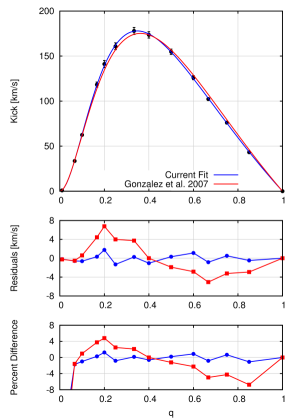
Figure 1: Our current fit and the original González et al. González et al. (2007) fit to the recoils from nonspinning BHBs. The panel below gives the residual and percent difference of both fits.

Table 5 gives the results of fitting the coefficients $A$, $B$, and $C$ in Eq. (1) to the 14 runs available here. We find that the value of the additional parameter $C$ is statistically significant and its inclusion improves the overall fit. In addition we compare the old González et al. (2007) $A,B$ parameters with our fit to just these two parameters, i.e. setting $C=0$ and find that they are close but the differences are statistically significant.

Table 5: Fitting to the recoil velocity of the remnant of nonspinning black hole binaries by Eq. (1). Fit 2 only uses $A,B$ while Fit 3 also fits $C$. Standard error for each fit is also given.

Parameter	Fit González et al. (2007)	Fit 2	Fit 3
$A$	$-9210$	$-8917\pm 73$	$-8695\pm 53$
$B$	$-2790$	$-4285\pm 261$	$-6683\pm 424$
$C$	$0.0$	$0.0$	$4179\pm 702$

We find that the maximum of the new fitting function lies at $q=0.348$ with a recoil velocity of $178$km/s which shifts the maximum to slightly lower mass ratio and slightly higher recoil velocity. The Gonzalez et al. fit finds a maximum recoil velocity of $175$km/s for $q=0.362$.

III.2 Peak luminosity of non-Spinning Binaries

The formula to model the peak luminosity introduced in Healy and Lousto (2017) takes the following simple form for nonspinning binaries

$$L_{\rm peak}=(4\eta)^{2}\,\Big{\{}N_{0}+N_{2d}\,\delta{m}^{2}+N_{4f}\,\delta{m}^{4}\Big{\}}.$$ (2)

Note that the radiated power in the particle limit scales as $\eta^{2}$ [see Ref. Fujita (2015), Eq. (16) and (20); evaluated at the ISCO for its peak value].

The results of fitting the parameters $N_{0}$, $N_{2d}$, and $N_{4f}$ to the peak luminosity of our 14 simulations is displayed in Fig. 2 and compared to the previous fit in Ref. Healy and Lousto (2017) (note that Healy and Lousto (2017) included spinning and nonspinning simulations to determine the fitting parameters). We summarize the results in Table 6.

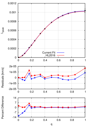
Figure 2: Our current fit and previous fit Healy and Lousto (2017) to the peak luminosity from nonspinning BHBs.

The results of this comparison is again a reduction of the residuals over the mass ratio range studied here and provides new values to the fitting parameters $N_{0},N_{2d},N_{4f}$ to be used in future hierarchical approaches to formulate the modeling of the more general case of spinning precessing black hole binaries. Note that increasing the resolution leads to an increase in the peak luminosity (likely due to the decreased effects of artificial dissipation at high resolution) This is reflected in the residuals over the whole range of the mass ratios, $q=1$ to $q=1/100$. The peak luminosity values reach a maximum for equal mass binaries, producing a peak just above $10^{-3}$ in dimensionless units and vanishing in the particle limit as $\eta^{2}$.

Table 6: The fitting coefficients for the peak luminosity Eq. (2).

Parameter	$L_{peak}$
$N_{0}$	$\ 1.029\times 10^{-3}\pm 2.454\times 10^{-6}$
$N_{2d}$	$-4.474\times 10^{-4}\pm 4.045\times 10^{-5}$
$N_{4f}$	$\ 3.086\times 10^{-4}\pm 9.310\times 10^{-5}$

III.3 Peak frequency and amplitude of non-Spinning Binaries

Analogously to the previous formula to model the peak luminosity, we introduce the following fitting formula for the peak frequency of the $(2,2)$ mode of the gravitational wave strain for nonspinning binaries

$$m\omega_{22}^{\mathrm{peak}}=\Big{\{}W_{0}+W_{2}\,\delta{m}^{2}+W_{4}\,\delta{m}^{4}\Big{\}},$$ (3)

The results of fitting the parameters $W_{0}$, $W_{2}$, and $W_{4}$ to the peak frequency of our 14 simulations are given in Table 7 and are displayed in Fig. 3. We note here that in the $q\to 0$ limit, the frequency approaches a value of $\approx 0.2807$, which is close to the particle limit $0.2795$ reported in the Bohé et al. (2017), Eq. (A6) [and to (twice) the frequency of the “ibco”, $0.25$ that innermost bounded circular orbit for nonspinning black holes Bardeen et al. (1972)]. While towards the equal-mass limit the frequency increases to $W_{0}\sim 0.358$. Note that Bohé et al. (2017) [Eq. (A7)] finds a peak frequency of $0.36$ in the equal-mass limit.

Table 7: Fitting to the peak frequency of the 22 mode of the strain produced by black hole binaries by Eq. (3) and Eq. (4). Standard error for each fit is also given.

Parameter	Fit 1	Parameter	Fit 2
$W_{0}$	$0.3586\pm 0.0008$	$W^{\prime}_{0}$	$0.3579\pm 0.0011$
$W_{2}$	$-0.1210\pm 0.0037$	$W^{\prime}_{2}$	$0.2471\pm 0.0094$
$W_{4}$	$0.0431\pm 0.0034$	$W^{\prime}_{4}$	$0.2713\pm 0.0129$

If we impose the particle limit peak frequency, $m_{f}\,\Omega_{p}=0.2795$ into our formula, we have the alternative Fit 2:

$$m\omega_{22}^{\mathrm{peak}}=(4\eta)\,\Big{\{}W^{\prime}_{0}+W^{\prime}_{2}\,\delta{m}^{2}+W^{\prime}_{4}\,\delta{m}^{4}\Big{\}}+m_{f}\,\Omega_{p}\,\delta{m}^{6},$$ (4)

where $\eta=(1-\delta{m}^{2})/4$.

Note also that the peak frequency for the Weyl scalar $\psi_{4}$ (instead of the strain $h$ studied here), was studied in Healy et al. (2014b) in connection with the quasinormal modes of the final remnant and a fitting to the peak frequency produced by numerical simulations was used to calibrate EOB models in Taracchini et al. (2012).

Table 8: Fitting to the peak amplitude of the 22 mode of the strain produced by black hole binaries by Eq. (5). Standard error for each fit is also given.

Parameter	$r/mH_{22}^{peak}$
$H_{0}$	$0.3980\pm 0.0003$
$H_{2}$	$-0.0558\pm 0.0019$
$H_{4}$	$0.0183\pm 0.0019$

In addition to modeling the peak frequency, We also model the peak amplitude (of the strain $h$) from the merger of nonspinning binaries using the expansion

$$h_{\rm peak}=(4\eta)\,\Big{\{}H_{0}+H_{2}\,\delta{m}^{2}+H_{4}\,\delta{m}^{4}\Big{\}}.$$ (5)

The results from this fit are summarized in Table 8 and Fig. 4.

Figure 3: Current fit and the Bohé et al. Bohé et al. (2017) fit to the peak waveform frequency from nonspinning BHBs.

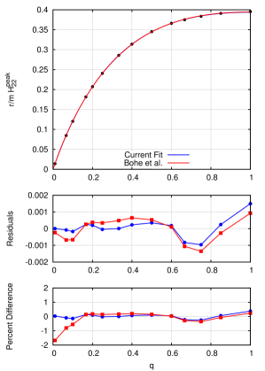
Figure 4: Current fit and the Bohé et al. Bohé et al. (2017) fit to the peak strain amplitude from nonspinning BHBs.

IV Conclusions and Discussion

The study of remnant formulas has been of interest since the pioneering work using the Lazarus approach Baker et al. (2004); Campanelli (2005) over a decade ago. The breakthroughs in numerical relativity allowed for a more complete study and a number of increasingly general and accurate phenomenological formulas have been put forward over the years (See for instance Lousto et al. (2010c); Lousto and Zlochower (2014); Hofmann et al. (2016); Jimńez-Forteza et al. (2017) and references therein). The first detection of gravitational waves from the merger of two black holes Abbott et al. (2016a) produced a renewed interest in the remnant formulas Abbott et al. (2016f, e, d, b, c).

The remnant formulas for the final mass and spin of the product of two merged black holes can be made very accurately since we can compute the final masses and spins (magnitudes) from the isolated horizon formulas Dreyer et al. (2003b). Alternatively, one can compute those quantities from the energy and angular momentum carried out to infinity by the waveforms and subtract those values from the initial total mass and angular momentum of the system. This method, provides a consistency check to the isolated horizon computation, but requires higher resolutions to achieve comparable accuracy (See appendices in Refs. Healy et al. (2014a); Healy and Lousto (2017)). A third method can be also used by measuring directly the quasinormal modes in the late ringdown phase of the waveform and relate them to the mass and spin of a perturbed Kerr black hole (See for instance Table III in Dain et al. (2008) and references therein).

The recoil velocity of the remnant and the peak luminosity of merging binary black holes is also of renewed interest Keitel et al. (2016); Healy and Lousto (2017) but those quantities (as well as the peak frequency and amplitude) are computed from the waveforms (but see Krishnan et al. (2007)) and hence are computed with less accuracy in the routine simulations that do not reach ultra-high resolutions. In this paper, we have revisited the study of nonspinning binaries with a set of three resolutions (low, medium, high) that allows us to confirm that we are in the convergence regime and that we are able to extrapolate to infinite resolution to obtain a more accurate recoil and peak luminosity than by the standard runs Healy and Lousto (2017). This serves to establish a new set of fitting coefficients that, in a hierarchical approach, will serve as fixed constants in the new fittings (or refitting) of the more general remnant formulas (for the spinning Healy and Lousto (2017) and precessing Zlochower and Lousto (2015) binaries). We have also introduced formulas for the gravitational wave frequency and amplitude at the peak of the strain. This provides further information about the full numerical simulations that can be used Bohé et al. (2017) to improve the approximate modeling of gravitational waveforms used for data analysis of gravitational wave signals measured by laser interferometric detectors. The fittings (2)-(5) can also be used for a consistency test of general relativity by comparing the prediction of the peak luminosity/amplitude and the frequency of this peak from the above formulas (and its generalization to spinning black holes) with an actual measurement from a gravitational wave signal Cornish and Littenberg (2015); Klimenko et al. (2016); Lynch et al. (2015); B csy et al. (2016); Abbott et al. (2016g).