Fundamental mode exact schemes for unsteady problems

Abstract

The problem of increasing the accuracy of an approximate solution is considered for boundary value problems for parabolic equations. For ordinary differential equations (ODEs), nonstandard finite difference schemes are in common use for this problem. They are based on a modification of standard discretizations of time derivatives and, in some cases, allow to obtain the exact solution of problems. For multidimensional problems, we can consider the problem of increasing the accuracy only for the most important components of the approximate solution. In the present work, new unconditionally stable schemes for parabolic problems are constructed, which are exact for the fundamental mode. Such two-level schemes are designed via a modification of standard schemes with weights using Padé approximations. Numerical results obtained for a model problem demonstrate advantages of the proposed fundamental mode exact schemes.

1 Introduction

In numerical solving time-dependent boundary value problems, the emphasis is on using computational algorithms of higher accuracy (see, e.g., [1, 2]). Along with increasing the accuracy of discretization in space, increasing the accuracy of discretization in time is also considered taking into account numerical methods developed for ordinary differential equations [3, 4]. In view of features of unsteady problems for partial differential equations, we, first of all, should be guided by methods of numerical solving Cauchy problems for stiff systems of ordinary differential equations [5, 6].

As a rule, discretization in time for numerical solving boundary value problems for parabolic equations is constructed on the basis of two- or three-level schemes. To study stability of such difference schemes, the theory of stability and well-posedness for operator-difference schemes [7, 8] is employed. In particular, stability conditions for standard schemes with weights ($\theta$-method) are obtained for linear problems in different Hilbert spaces. For two-level schemes, where the solution at two consecutive time levels is involved, polynomial approximations are explicitly or implicitly employed for operators of difference schemes. The Runge-Kutta methods (see [6, 9]) are well-known examples of such schemes widely used in modern computational practice. The main feature of multilevel schemes (multistep methods) results in the approximation of time derivatives with higher accuracy on a multipoint stencil. Multistep methods based on numerical backward differentiation formulas [10] should be mentioned as a typical example.

In some cases, it is possible to construct exact difference schemes. The main possibilities of their construction for solving Cauchy problems for ordinary differential equations are reflected in the works [11, 12, 13]. The idea of increasing accuracy by modifying approximations of time derivatives can be realized not only for linear equations, but also for nonlinear ones and for systems of equations. Separately, we highlight the works [14, 15, 16, 17], where such a technology of constructing discretization in time is applied to solving parabolic equations. Using perturbations with a low parameter for standard difference approximations, we can provide a new quality of the solution, which is associated, for example, with the fulfillment of some conservation law.

For a Cauchy problem for a homogeneous linear parabolic equation, the solution can be represented as a superposition of modes, which are associated with the corresponding eigenfunctions of the elliptic operator. Dominant modes are the most important, since higher modes decay very quickly. Such a qualitative behavior of the solution must hold for a discrete problem as well. For long times, the fundamental mode of the solution is highlighted, when a regular regime is considered (see, e.g., [18]). In the theory of difference schemes [19], there is recognized a class of asymptotically stable difference schemes that provide the correct behavior of the approximate solution for large times. SM (Spectral Mimetic) properties of operator-difference schemes for numerical solving the Cauchy problem for evolutionary equations of first order are associated with the time-evolution of individual modes of the solution. For long times, the fundamental mode of the solution is highlighted for a regular regime. With this in mind, SM-stable difference schemes are constructed [20].

Here we construct difference schemes for parabolic equations, which are exact for the most important component of the solution, namely, the fundamental mode is calculated exactly. Two-level fundamental mode exact schemes (FMES) are constructed using Padé approximations.

The paper is organized as follows. A boundary value problem for a linear parabolic equation with a self-adjoint elliptic operator of second order is considered in Section 2. Using finite element approximations in space, we formulate a Cauchy problem for the corresponding differential-operator equation. In Section 3, we consider standard two-level schemes with weights and formulate stability conditions. Schemes that are exact for the solution associated with the fundamental eigenfunction of the corresponding elliptic operator are constructed in Section 4. Section 5 presents the results of numerical experiments on studying FMES accuracy for a model initial-boundary value parabolic problem.

2 Problem statement

Let $\Omega$ be a bounded domain ($\Omega\subset\mathbb{R}^{d},d=2,3$) with a piecewise smooth boundary $\partial\Omega$. Define an elliptic operator $\mathcal{A}$ such that

$$\mathcal{A}u:=-\nabla(k(\bm{x})\nabla u)+c(\bm{x})u,\quad\bm{x}\in\Omega.$$ (1)

The operator $A$ is defined on the set of functions $u({\bm{x}})$ that satisfy on the boundary $\partial\Omega$ the following conditions:

$$k({\bm{x}})\frac{\partial u}{\partial n}+\mu({\bm{x}})u=0,\quad{\bm{x}}\in\partial\Omega.$$ (2)

Coefficients $k(\bm{x})$, $c(\bm{x})$ and $\mu({\bm{x}})$ are smooth functions in $\overline{\Omega}$ and

$$k(\bm{x})\geq\kappa>0,\quad\mu(\bm{x})\geq 0,\quad\bm{x}\in\Omega.$$

We consider the Cauchy problem

$$\frac{du}{dt}+\mathcal{A}u=0,\quad 0<t\leq T,$$ (3)

$$u(0)=u^{0},$$ (4)

where, for example, $u^{0}(\bm{x})\in L_{2}(\Omega)$ with the notation $u(t)=u(\bm{x},t)$.

Let $(\cdot,\cdot),\|\cdot\|$ be the scalar product and norm in $H=L_{2}(\Omega)$, respectively:

$$(u,v):=\int_{\Omega}u({\bm{x}})v({\bm{x}})d{\bm{x}},\quad\|u\|:=(u,u)^{1/2}.$$

Multiplying equation (3) by $v(\bm{x})\in H^{1}(\Omega)$ and integrating over the domain $\Omega$, we arrive at the equality

$$\left(\frac{du}{dt},v\right)+a(u,v)=0,\quad\forall v\in H^{1}(\Omega),\quad 0<t\leq T.$$ (5)

Here $a(\cdot,\cdot)$ is the following bilinear form:

$$a(u,v):=\int_{\Omega}(k\nabla u\cdot\nabla v+c\,u\,v)d\bm{x}+\int_{\partial\Omega}\mu\,u\,v\,d\bm{x},$$

where

$$a(u,v)=a(v,u),\quad a(u,u)\geq\delta\|u\|^{2},$$

with a constant $\delta$. In view of (4), we put

$$(u(0),v)=(u^{0},v),\quad\forall v\in H^{1}(\Omega).$$ (6)

The variational (weak) formulation of the problem (1)–(4) consists in finding $u(\bm{x},t)\in H^{1}(\Omega)$, $0<t\leq T$ that satisfies (5), (6) with the condition (2) on the boundary.

For the solution of the problem (5), (6), we have the a priori estimate

$$\|u(t)\|\leq\exp(-\delta t)\|u^{0}\|.$$ (7)

To show this, we put $v=u$ in (5) and get

$$\|u\|\frac{d}{dt}\|u\|+a(u,u)=0.$$

Taking into account the lower bound for the bilinear form $a(\cdot,\cdot)$, we get

$$\frac{d}{dt}\|u(t)\|+\delta\|u(t)\|\leq 0.$$

From this inequality, in view of (6), it follows that the estimate (7) holds.

For numerical solving the initial-boundary value problem (3), (4), discretization in space is constructed using the finite element method [21, 22]. The weak formulation (5), (6) is employed. Define the subspace of finite elements $V^{h}\subset H^{1}(\Omega)$ and the discrete elliptic operator $A$ as

$$(Ay,v)=a(y,v),\quad\forall\ y,v\in V^{h}.$$

The operator $A$ acts on the finite dimensional space $V^{h}$ and

$$A=A^{*}\geq\delta_{h}I,$$ (8)

where $I$ is the identity operator.

For the problem (3), (4), we put into the correspondence the operator equation for $w(t)\in V^{h}$:

$$\frac{dw}{dt}+Aw=0,\quad 0<t\leq T,$$ (9)

$$w(0)=w^{0},$$ (10)

where $w^{0}=Pu^{0}$ with $P$ denoting $L_{2}$-projection onto $V^{h}$. Similarly to (7), we establish the estimate

$$\|w(t)\|\leq\exp(-\delta_{h}t)\|w^{0}\|$$ (11)

for the solution of the problem (9), (10).

To solve the problem (9), (10), the separation of variables method is applied. For the spectral problem

$$A\varphi_{k}=\lambda_{k}\varphi_{k}$$

we have real eigenvalues

$$\lambda_{1}\leq\lambda_{2}\leq...\leq\lambda_{M_{h}}.$$

The eigenfunctions $\varphi_{k},\ \|\varphi_{k}\|=1,\ k=1,2,...,M_{h}$ form a basis in $V^{h}$. Therefore, for $y\in V^{h}$, we have

$$y=\sum_{k=1}^{M_{h}}y_{k}\varphi_{k},\quad y_{k}=(y,\varphi_{k}),\quad k=1,2,...,M_{h}.$$

In view of this, the solution of the problem (9), (10) is represented in the form

$$w(\bm{x},t)=\sum_{k=1}^{M_{h}}w_{k}^{0}\exp(-\lambda_{k}t)\varphi_{k}(\bm{x}).$$ (12)

With this representation, we get the a priori estimate (1) with $\delta_{h}=\lambda_{1}$.

Various effects arising from modes can be taken into account in constructing difference schemes. Assume that the fundamental mode is separated from other modes, i.e., $\lambda_{1}<\lambda_{2}$. Then, for large times, a regular regime is established for the solution:

$$w(\bm{x},t)\approx w_{1}^{0}\exp(-\lambda_{1}t)\varphi_{1}(\bm{x}).$$

If such a property is preserved after discretization in time, then we speak of asymptotic stability of difference schemes [19]. In the representation (12), higher modes decay faster with time. Such a monotone behavior of different modes is inherited in SM-stable difference schemes [20].

It seems natural to construct discretizations in time that are more accurate in reproducing the time dependence of dominant modes. In particular, we distinguish nonstandard difference schemes, which are exact for the fundamental mode of the solution, namely, fundamental mode exact schemes.

3 Nonstandard schemes with weights

The standard approach to the solution of the problem (9), (10) is associated with using two-level schemes. Let $\tau$ be a step of a uniform grid in time such that $y^{n}=y(t^{n}),\ t^{n}=n\tau$, $n=0,1,...,N,\ N\tau=T$. For a constant weight parameter $\sigma\ (0<\sigma\leq 1)$, we approximate equation (9) by the following two-level scheme:

$$\frac{y^{n+1}-y^{n}}{\tau}+A(\sigma y^{n+1}+(1-\sigma)y^{n})=0,\quad n=0,1,...,N-1,$$ (13)

with the initial conditions

$$y^{0}=w^{0},$$ (14)

where $\sigma$ is a parameter (weight). If $\sigma=0$, then (13), (14) becomes the explicit scheme, for $\sigma=1$, we obtain the fully implicit scheme, whereas $\sigma=0.5$ corresponds to the symmetric (Crank–Nicolson) scheme.

Similarly to (12), the solution of the problem (13), (14) can be represented as

$$y^{n}=\sum_{k=1}^{M_{h}}y^{n}_{k}\varphi_{k},\quad n=0,1,...,N.$$ (15)

Substitution of (15) into (13) results in the following relation for an individual mode:

$$y^{n+1}_{k}=r(\sigma,\lambda_{k}\tau)y^{n}_{k},\quad k=1,2,...,M_{h},\quad n=0,1,...,N-1,$$

where

$$r(\sigma,\eta):=\frac{1-(1-\sigma)\eta}{1+\sigma\eta}.$$

The scheme (13), (14) belongs to the class of FMES, if the following condition holds:

$$y^{n+1}_{1}=\exp(-\lambda_{1}\tau)y^{n}_{1}.$$ (16)

For any $\sigma$, the equation

$$r(\sigma,\eta_{1})=\exp(-\eta_{1}),\quad\eta_{1}=\lambda_{1}\tau$$

does not hold. Thus, for the schemes with weights (13), (14), there is not any fundamental mode exact scheme.

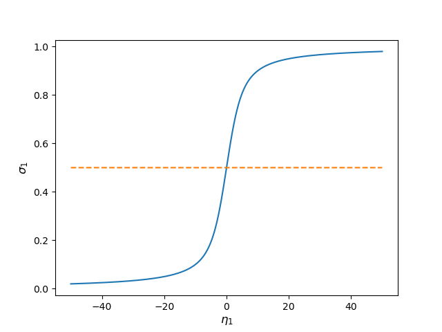
Figure 1: Weight value for FMES.

It is possible to select a weight value in such a way that the fundamental mode is calculated exactly. The value $\sigma_{1}$ such that $r(\sigma_{1},\eta_{1})=\exp(-\eta_{1})$ is shown in Fig. 1. We restrict ourselves to the values $|\eta_{1}|\ll 1$. In the most important case, we have $\sigma_{1}\approx 0.5$. For computational practice, the fully implicit scheme ($\sigma=1$) is more interesting, but it cannot describe accurately the time-variation of the fundamental mode.

In our previous work [23], special unconditionally stable schemes were constructed for convection-diffusion problems using a transition to new unknowns. The main feature of these schemes is connected with the negativity of the constant $\delta_{h}$ in the lower bound for the operator $A$ (the estimate (8) in the present work). Here we use this idea for constructing fundamental mode exact schemes.

For the solution of the problem (9), (10), we apply the representation

$$w(t)=\exp(-\lambda_{1}t)v(t).$$ (17)

Substitution of (17) into (9), (10) results in the problem

$$\frac{dv}{dt}+\widetilde{A}v=0,\quad 0<t\leq T,$$ (18)

$$v(0)=w^{0},$$ (19)

where

$$\widetilde{A}:=A-\lambda_{1}I,$$ (20)

and

$$\widetilde{A}=\widetilde{A}^{*}\geq 0.$$

For the problem (18), (19), we use the standard scheme with weights:

$$\frac{g^{n+1}-g^{n}}{\tau}+\widetilde{A}(\sigma g^{n+1}+(1-\sigma)g^{n})=0,\quad n=0,1,...,N-1,$$ (21)

$$g^{0}=w^{0}.$$ (22)

In view of (17), suppose that $y^{n}=\exp(-\lambda_{1}t^{n})g^{n}$. Thus, we arrive at the scheme

$$\frac{\exp(\lambda_{1}\tau)y^{n+1}-y^{n}}{\tau}+\widetilde{A}(\sigma\exp(\lambda_{1}\tau)y^{n+1}+(1-\sigma)y^{n})=0,\quad n=0,1,...,N-1,$$ (23)

with the initial condition

$$y^{0}=w^{0}.$$ (24)

This is a new scheme for the initial problem (9), (10).

A comparison of the nonstandard scheme (20), (23), (24) with the standard scheme with weights (13), (14) indicates that we modified not only discretization in time, but also the problem operator itself:

$$y^{n+1}\rightarrow\exp(\lambda_{1}\tau)y^{n+1},\quad A\rightarrow A-\lambda_{1}I.$$ (25)

Using the representation (15), we obtain

$$\frac{\exp(\lambda_{1}\tau)y_{1}^{n+1}-y_{1}^{n}}{\tau}=0.$$

Thus, the condition (16) is fulfilled and this scheme is of FMES-type.

The nonstandard scheme (20), (23), (24) is unconditionally stable under the standard restriction on the weight $\sigma\geq 0.5$. The proof is based on the well-known (see, e.g., [7, 8]) condition for the stability of the scheme with weights (21), (22). Multiply equation (18) scalarly by

$$\sigma g^{n+1}+(1-\sigma)g^{n}=\tau\left(\sigma-\frac{1}{2}\right)\frac{g^{n+1}-g^{n}}{\tau}+\frac{1}{2}(g^{n+1}+g^{n}).$$

In view of $\widetilde{A}\geq 0$, we get

$$\tau\left(\sigma-\frac{1}{2}\right)\left\|\frac{g^{n+1}-g^{n}}{\tau}\right\|^{2}+\frac{1}{2\tau}(\|g^{n+1}\|^{2}-\|g^{n}\|^{2})\leq 0.$$

Thus, for $\sigma\geq 0.5$, we have

$$\|g^{n+1}\|\leq\|g^{n}\|\leq...\leq\|w^{0}\|.$$

Using the relation between $y^{n}$ and $g^{n}$, we obtain for the scheme (23), (24) the a priori estimate

$$\|y^{n+1}\|\leq\exp(-\lambda_{1}t^{n+1})\|w^{0}\|,\quad n=0,1,...,N-1.$$ (26)

This estimate is consistent with the estimate (11) for the problem (9), (10), since $\delta_{h}=\lambda_{1}$. Thus, we arrive at the following statement.

Theorem 1

The difference scheme (20), (23), (24) is a fundamental mode exact scheme. It is unconditionally stable for $\sigma\geq 0.5$ and the estimate (26) holds.

4 Schemes based on Padé approximations

Two-level finite difference schemes of higher approximation order for time-dependent linear problems can be conveniently constructed on the basis of Padé approximations for the corresponding operator (matrix) exponential function [24]. In the case of linear systems of ODEs, such approximations correspond to various variants of the Runge-Kutta method [5, 6, 9].

The solution of the problem (9), (10) can be represented as

$$w(t)=\exp(-At)w^{0},\quad 0<t\leq T,$$

and so

$$w(t^{n+1})=\exp(-A\tau)w(t^{n}),\quad n=0,1,...,N-1.$$

For the corresponding difference scheme, we have

$$y^{n+1}=Sy^{n},\quad n=0,1,...,N-1,$$ (27)

with the operator of transition to a new time level $S=s(-A\tau)$. For (27), we have the representation (15), where now we have

$$y^{n+1}_{k}=s(\lambda_{k}\tau)y^{n}_{k},\quad k=1,2,...,M_{h},\quad n=0,1,...,N-1.$$

It is necessary to choose one or another function $s(z)$, which approximates the function $\exp(-z)$ for$z\geq z_{0}$, where $z_{0}=\lambda_{1}\tau$. To obtain an exact scheme for the fundamental mode, we must (see (16)) fulfill $s(z_{0})=\exp(-z_{0})$.

The Padé approximation of the function $\exp(-z)$ is

$$\exp(-z)=R_{lm}(z)+\mathcal{O}(z^{l+m+1}),\quad R_{lm}(z)=\frac{P_{lm}(z)}{Q_{lm}(z)},$$ (28)

where $P_{lm}(z)$ and $Q_{lm}(z)$ are polynomials of degrees $l$ and $m$, respectively. These polynomials have [25] the form

$$P_{lm}(z):=\frac{l!}{(l+m)!}\sum_{k=0}^{l}\frac{(l+m-k)!}{k!(l-k)!}(-z)^{k},$$

$$Q_{lm}(z):=\frac{m!}{(l+m)!}\sum_{k=0}^{m}\frac{(l+m-k)!}{k!(m-k)!}z^{k}.$$

At the point $z=0$ the approximation is exact, i.e. $\exp(0)=R_{lm}(0)$. We search the exact approximation at the point $z_{1}=\eta_{1}=\lambda_{1}\tau$. Taking this into account, we put

$$\exp(-z)\approx\exp(-z_{1})R_{lm}(\widetilde{z}),\quad\widetilde{z}=z-z_{1}.$$

The fundamental mode exact scheme based on Padé approximations can be represented in the form (27), where in view of (20) and (28), we have

$$S=\exp(-\lambda_{1}\tau)R_{lm}(\widetilde{A}\tau).$$ (29)

In fact, this means that the transformation (25) is realized. Thus, we can formulate the following statement.

Theorem 2

The difference schemes (20), (24), (27), (29) based on Padé approximations belong to the class of fundamental mode exact schemes.

Let us highlight the most interesting variants of the constructed schemes of FMES-type. The scheme (27), (29) with $l=0,m=1$ corresponds to the fully implicit scheme ($\sigma=1$ in(23), (24)). The scheme (27), (29) with $l=1,m=1$ is associated with the Crank-Nicolson scheme ($\sigma=0.5$ in (23), (24)).

Only the schemes with $l=0$, i.e.,

$$R_{0m}(z)=\frac{1}{Q_{0m}(z)},\quad P_{0m}(z)=1$$

are SM-stable [20]. In this case, the two-level difference scheme for the problem (9), (10) is

$$\frac{\exp(\lambda_{1}\tau)y^{n+1}-y^{n}}{\tau}+\frac{1}{\tau}(Q_{0m}(\widetilde{A}\tau)-I)y^{n+1}=0,\quad n=0,1,...,N-1,$$ (30)

where the function

$$Q_{0m}(z)=\sum_{k=0}^{m}\frac{1}{k!}z^{k}$$

is a truncated Taylor series for $\exp(z)$.

In the class of schemes (30), in addition to the fully implicit scheme of the first-order approximation in time ($m=1$), we highlight the scheme with $m=2$. In this case, the approximate solution is determined from

$$\frac{\exp(\lambda_{1}\tau)y^{n+1}-y^{n}}{\tau}+\left(\widetilde{A}+\frac{\tau}{2}\widetilde{A}^{2}\right)y^{n+1}=0,\quad n=0,1,...,N-1.$$ (31)

It has, like the Crank-Nicolson scheme ($\sigma=0.5$ in (23), (24)), the second-order approximation in time, but, as an SM-stable scheme, it reproduces more accurately the behavior of higher modes.

5 Numerical experiments

Figure 2: Computational domain, coefficients of the equation and the boundary conditions

The model problem (1)–(4) is considered in the unit square ($\Omega=[0,1]\times[0,1]$). We assume that $c(\bm{x})=c=\mathrm{const}$, and the coefficient $k(\bm{x})$ in equation (1) is discontinuous. Namely, in the left lower quarter of the computational domain $\Omega$, it is equal to 10, in other parts of the region it equals 1. Neumann-type or Robin-type boundary conditions are specified on different parts of the boundary. The values of the coefficient $k(\bm{x})$ and function $\mu(\bm{x})$ in the boundary condition (2) are shown in Fig. 2. Thus, we consider the problem (3), (4), where

$$\mathcal{A}=\bar{\mathcal{A}}+cI,\quad\bar{\mathcal{A}}u:=-\nabla(k(\bm{x})\nabla u),\quad\bm{x}\in\Omega.$$

A uniform grid in space $N_{h}\times N_{h}$ is used. Piecewise-linear finite elements on triangles are employed.

The constructed nonstandard difference schemes are based on using the known fundamental eigenvalue $\delta=\lambda_{1}$. The computation of the first eigenvalues and the corresponding eigenfunctions is the standard problem of computational mathematics [26]. We can focus on applying well-designed algorithms and relevant open-source software. To solve the spectral problems, we recommend the SLEPc package (Scalable Library for Eigenvalue Problem Computations, http://slepc.upv.es/). In this library, in particular, there are implemented the Krylov-Schur algorithm and a variant of the Arnoldi method proposed by [27].

We apply, for example, the standard inverse iteration method to find the fundamental eigenvalue of the spectral problem:

$$\bar{A}\varphi=\bar{\lambda}\varphi.$$

In the simplest case, we can put $\varphi^{0}$ as the initial value. At the $m+1$-st iteration, we have

$$\bar{A}\varphi^{m+1}=\varphi^{m}.$$ (32)

For the $m+1$-st approximate values of the first eigenvalue and the corresponding eigenfunction, we get

$$\bar{\lambda}_{1}^{m+1}=\frac{(\varphi^{m},\varphi^{m})}{(\varphi^{m+1},\varphi^{m})},\quad\varphi^{m+1}_{1}=\frac{\varphi^{m+1}}{\|\varphi^{m+1}\|}.$$

For the operator $A=\bar{A}+cI$, we have the same eigenfunctions, and $\lambda_{1}=\bar{\lambda}_{1}+c$. The fast convergence of the inverse iteration method for the simplest variant (32) is presented in Table 1. The calculations are performed on the sequence of grids derived via dividing the size of triangles by half. A small number of iterations is enough to find the first eigenvalue and the corresponding eigenfunction. The first eigenfunction on the grid with $N_{h}=51$ is shown in Fig. 3. The solution value on contour levels is a multiple of $0.1$.

Table 1: Iterative approximation to the first eigenvalue

$m$	$N_{h}=26$	$N_{h}=51$	$N_{h}=101$
1	5.48146728860	5.41108707044	5.40129163974
2	4.62435922303	4.54593036350	4.54096438823
3	4.61225694503	4.53300663413	4.52815998124
4	4.61203189452	4.53275210569	4.52790926702
5	4.61202756655	4.53274692872	4.52790419871
6	4.61202748265	4.53274682270	4.52790409555
7	4.61202748102	4.53274682052	4.52790409345
8	4.61202748099	4.53274682048	4.52790409341
9	4.61202748099	4.53274682048	4.52790409340
10	4.61202748099	4.53274682048	4.52790409340

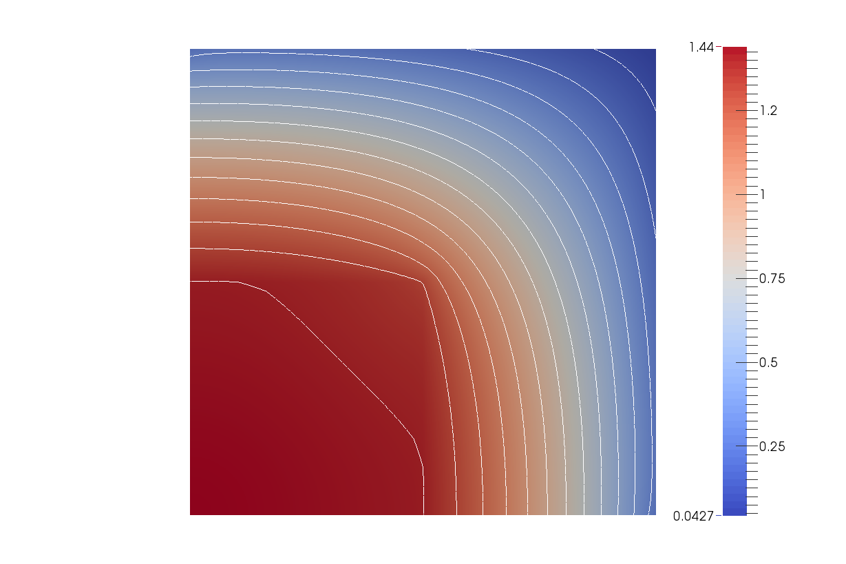
Figure 3: Fundamental eigenfunction.

The time-dependent problem is considered until $T=0.1$. The initial condition (4) is taken in the form $u^{0}(\bm{x})=1,\ \bm{x}\in\Omega$. For the basic variant, we put $c=0$. We compare the standard fully implicit scheme (($\sigma=1$ in (13)) and the nonstandard scheme (23) with the same value $\sigma$. The accuracy of calculating the amplitude of the fundamental mode is estimated by the following value:

$$\varepsilon_{a}(t^{n})=(y^{n},\varphi_{1})-(y^{0},\varphi_{1})\exp(-\lambda_{1}t^{n}),\quad n=0,1,...,N.$$

Numerical results for the amplitude of the fundamental mode obtained on different grids in time are given in Fig. 4.

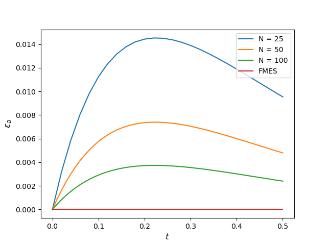
Figure 4: Time-variation the amplitude of the fundamental mode.

It is possible to evaluate the general error of the approximate solution without separating the fundamental mode. As a reference solution (the benchmark solution used for a comparison) we employ the solution $\bar{y}$ that is obtained using the fully implicit scheme (13), (14) on the finest grid in time (the number of time steps is $N=1000$). The accuracy of the approximate solution is estimated at each time level:

$$\varepsilon_{u}(t^{n})=\frac{\|y^{n}-\bar{y}(t^{n})\|}{\|y^{n}\|},\quad n=0,1,...,N.$$

Numerical results for the fully implicit scheme (13), (14) are given in Fig. 5. Similar data for the nonstandard scheme (23), (24) for $\sigma=1$ are shown in Fig. 6. We observe a much higher accuracy of the approximate solution obtained using the FMES-type scheme. The influence of the constant $c$ is illustrated in Figs. 7 and 8. Obviously, the nonstandard scheme demonstrates higher accuracy in comparison with the standard scheme.

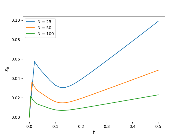
Figure 5: Accuracy of the standard fully implicit scheme.

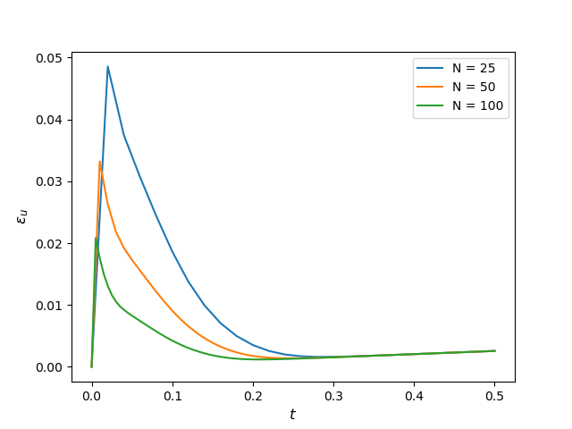
Figure 6: Accuracy of the nonstandard fully implicit scheme.

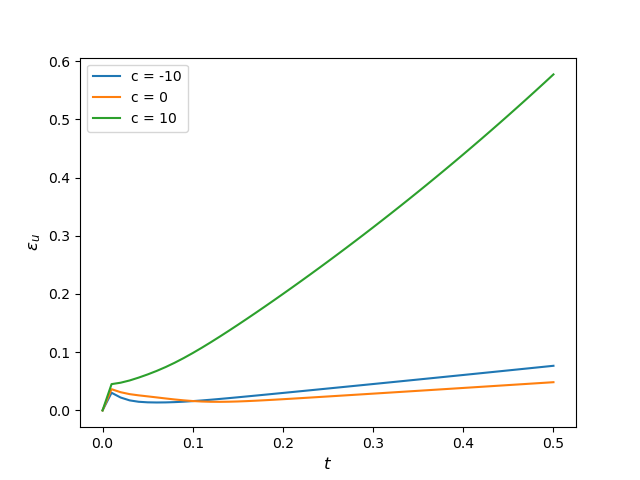
Figure 7: Accuracy of the standard fully implicit scheme for various values of $c$.

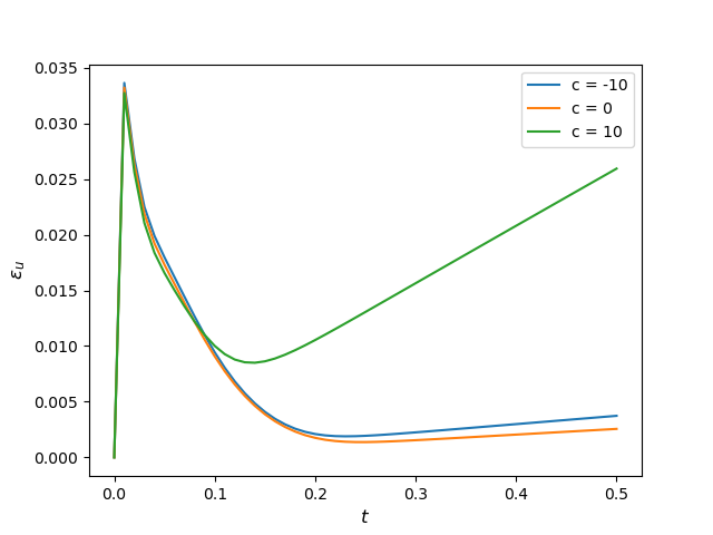
Figure 8: Accuracy of the nonstandard fully implicit scheme for various values of $c$.

References

- [1] W. H. Hundsdorfer, J. G. Verwer, Numerical Solution of Time-dependent Advection-diffusion-reaction Equations, Springer Verlag, 2003.
- [2] B. Gustafsson, High Order Difference Methods for Time Dependent PDE, Springer Verlag, 2008.
- [3] U. M. Ascher, Numerical Methods for Evolutionary Differential Equations, Society for Industrial Mathematics, 2008.
- [4] R. J. LeVeque, Finite Difference Methods for Ordinary and Partial Differential Equations: Steady-state and Time-dependent Problems, Society for Industrial Mathematics, 2007.
- [5] E. Hairer, G. Wanner, Solving Ordinary Differential Equations II: Stiff and Differential-algebraic Problems, Springer Verlag, 2010.
- [6] J. C. Butcher, Numerical Methods for Ordinary Differential Equations, Wiley, 2008.
- [7] A. A. Samarskii, The Theory of Difference Schemes, Marcel Dekker, New York, 2001.
- [8] A. A. Samarskii, P. P. Matus, P. N. Vabishchevich, Difference Schemes with Operator Factors, Kluwer Academic Publishers, 2002.
- [9] K. Dekker, J. G. Verwer, Stability of Runge-Kutta Methods for Stiff Nonlinear Differential Equations, North-Holland, Amsterdam, 1984.
- [10] C. W. Gear, Numerical Initial Value Problems in Ordinary Differential Equations, Prentice Hall, NJ, 1971.
- [11] R. E. Mickens, Nonstandard Finite Difference Models of Differential Equations, world scientific, 1994.
- [12] R. E. Mickens, Nonstandard finite difference schemes for differential equations, The Journal of Difference Equations and Applications 8 (9) (2002) 823–847.
- [13] R. Anguelov, J. M.-S. Lubuma, Contributions to the mathematics of the nonstandard finite difference method and applications, Numerical Methods for Partial Differential Equations 17 (5) (2001) 518–543.
- [14] R. E. Mickens, Nonstandard finite difference schemes for reaction-diffusion equations, Numerical Methods for Partial Differential Equations 15 (2) (1999) 201–214.
- [15] R. Anguelov, P. Kama, J.-S. Lubuma, On non-standard finite difference models of reaction–diffusion equations, Journal of computational and Applied Mathematics 175 (1) (2005) 11–29.
- [16] K. C. Patidar, On the use of nonstandard finite difference methods, Journal of Difference Equations and Applications 11 (8) (2005) 735–758.
- [17] E. Hernandez-Martinez, H. Puebla, F. Valdes-Parada, J. Alvarez-Ramirez, Nonstandard finite difference schemes based on Green’s function formulations for reaction–diffusion–convection systems, Chemical Engineering Science 94 (2013) 245–255.
- [18] A. Luikov, Analytical Heat Diffusion Theory, Academic Press, 1968.
- [19] A. A. Samarskii, P. N. Vabishchevich, Computational Heat Transfer, Wiley, 1996.
- [20] P. N. Vabishchevich, Two-level finite difference scheme of improved accuracy order for time-dependent problems of mathematical physics, Computational Mathematics and Mathematical Physics 50 (1) (2010) 112–123.
- [21] S. C. Brenner, R. Scott, The Mathematical Theory of Finite Element Methods, Springer, 2008.
- [22] V. Thomée, Galerkin Finite Element Methods for Parabolic Problems, Springer Verlag, 2006.
- [23] N. M. Afanas’eva, P. N. Vabishchevich, M. V. Vasil’eva, Unconditionally stable schemes for convection-diffusion problems, Russian Mathematics 57 (3) (2013) 1–11.
- [24] N. J. Higham, Functions of Matrices: Theory and Computation, SIAM, Philadelphia, 2008.
- [25] G. A. Baker, P. R. Graves-Morris, Padé Approximants, Cambridge University Press, 1996.
- [26] Y. Saad, Numerical Methods for Large Eigenvalue Problems, SIAM, 2011.
- [27] G. W. Stewart, A Krylov–Schur algorithm for large eigenproblems, SIAM Journal on Matrix Analysis and Applications 23 (3) (2001) 601–614.