Role of scalar mesons in the beam asymmetry of $p\bar{p}$ and $\Lambda\bar{\Lambda}$ photoproduction at JLab

Abstract

We suggest a description of the beam asymmetry in $p\bar{p}$ and $\Lambda\bar{\Lambda}$ photoproduction off the proton $\vec{\gamma}+p\to p\bar{p}+p$ and $\vec{\gamma}+p\to\Lambda\bar{\Lambda}+p$, takes into account the contribution of the scalar mesons $f_{0}(1370)$, $f_{0}(1500)$, and $f_{0}(1710)$. These scalars are considered as mixed states of a glueball and nonstrange and strange quarkonia in the framework based on the use of effective hadronic Lagrangians. Present results can be used to guide the possible search for this reaction by the GlueX Collaboration at JLab. Also, we did an estimate of contribution of heavier scalar meson states $f_{0}(2020)$, $f_{0}(2100)$, and $f_{0}(2200)$.

I Introduction

In this paper, we investigate the beam asymmetry in the $p\bar{p}$ and $\Lambda\bar{\Lambda}$ photoproduction due to the possible contribution of scalar mesons. This reactions are relevant to the physical program of the GlueX Collaboration (Hall D) at JLab. Note that the GlueX Collaboration recently reported AlGhoul:2017nbp measurements of the photon beam asymmetry for the $\pi^{0}$ and $\eta$ photoproduction $\vec{\gamma}p\to p\pi^{0}$ and $\vec{\gamma}p\to p\eta$ using a 9 GeV linear-polarized, tagged photon beam incident on a liquid hydrogen target. The asymmetries, measured as a function of the proton momentum transfer, possess greater precision than previous $\pi^{0}$ measurements and are the first measurements involving the $\eta$ meson in this energy regime. The results are compared with theoretical predictions Laget2011 ; Mathieu2015 ; Nys2017 ; Donnachie2016 based on $t$–channel, quasiparticle exchange and constrain the axial-vector component of the neutral meson production mechanism in these models.

In present manuscript, we consider gluonic excitations in the intermediate mesons through photoproduction reactions. When focusing on events without really observed mesons, the detection of the glueball or a glueball component in a hadron is significantly simplified. The glueball will be present in these processes via its mixing with nonstrange and strange quarkonia components Giacosa2005 ; Chatzis2011 . In particular, the scalar fields $f_{1}=f_{0}(1370)$, $f_{2}=f_{0}(1500)$, and $f_{3}=f_{0}(1710)$ are considered as mixed states of the glueball $G$ and non strange ${\cal N}$ and strange $S$ quarkonia Giacosa2005 ; Chatzis2011 $f_{i}=B_{i1}{\cal N}+B_{i2}G+B_{i3}S\,,\ i=1,2,3$, where the $B_{ij}$ are elements of the $3\times 3$ mixing matrix rotating bare states $({\cal N},G,S)$ into the physical scalar mesons $f_{i}$. Therefore, the glueball $G$ component will appear in the couplings of scalar mesons with photon and vector (axial) mesons and in the scalar meson propagators, which are the basic blocks for the calculation of the baryon-antibaryon photoproduction in our approach (see Fig. 1). Regarding the coupling of scalar mesons with $p\bar{p}$ and $\Lambda\bar{\Lambda}$ pairs, we proceed as follows (see details in Appendix):
1) We neglect by the coupling of glueball component to $p\bar{p}$ and $\Lambda\bar{\Lambda}$.
2) In case of $p\bar{p}$ photoproduction, we neglect by the coupling of strange quarkonia with $p\bar{p}$ and suppose that $f_{i}p\bar{p}$ couplings are dominated by the coupling of the nonstrange component of $f_{i}$ to nucleons.
3) In case of $\Lambda\bar{\Lambda}$ photoproduction, we take into account the couplings of both nonstrange and strange components of $f_{i}$ to $\Lambda$ hyperons.

Figure 1: Relevant diagrams describing the contribution of intermediate scalar mesons $f_{0}^{(i)}=$ $f_{0}(1370)$, $f_{0}(1500)$ and $f_{0}(1710)$ to the photoproduction of the $B\bar{B}$ pair through the exchange of vector $V^{(j)}=\rho^{0},\,\omega$ and axial-vector $A^{(j)}=b_{1},\,h_{1}$ mesons (or the corresponding Reggeons). Here, $W=V,A$ and $B=p,\Lambda$.

We start with definition of kinematics of the process of baryon-antibaryon photoproduction of the proton $\vec{\gamma}(q)+p(p)\to p(p^{\prime})+B(q_{1})+\bar{B}(q_{2})$ and introduce beam asymmetry: 1) $p$, $p^{\prime}$, $q$, $q_{1}$, and $q_{2}$ are the momenta of the initial and final protons, photon, produced baryon and antibaryon, respectively. 2) Invariant Mandelstam variables $s$ (total energy), $t$ (the square momentum transferred to the target proton), and $s_{2}$ (the square of the invariant mass of the produced $B\bar{B}$ pair) are defined as

$$s = (p+q)^{2}=(p^{\prime}+q_{1}+q_{2})^{2}\,,$$

$$t = k^{2}=(p^{\prime}-p)^{2}=(q-q_{1}-q_{2})^{2}\,,$$

$$s_{2} = (q_{1}+q_{2})^{2}\,.$$ (1)

3) The asymmetry $A_{B\bar{B}}$, written according to the known Basel convention as

$$A_{B\bar{B}}(t)=\frac{d\sigma_{\bot}/d\Omega-d\sigma_{||}/d\Omega}{d\sigma_{\bot}/d\Omega+d\sigma_{||}/d\Omega}=P_{\gamma}\Sigma\cos{2\varphi}$$ (2)

can be measured experimentally at JLab in a large interval of $t$. The numerator on the rhs of Eq. (2) is the difference of cross sections measured for linearly polarized photons, $\sigma_{||}$ for the polarization along the $x$ axis and $\sigma_{\bot}$ for the polarization along the $y$ axis, which are named the “PARA” and “PERP” orientations, respectively. The asymmetry $A_{B\bar{B}}(t)$ of Eq. (2) includes the factor $P_{\gamma}$ (the linear polarization of the initial photon beam), and thus the coefficient $\Sigma$ only can be considered as a beam asymmetry of the physical process. 4) We use the laboratory (Lab) frame with the $z$ axis directed along the photon momentum $q^{\mu}=\{|\bm{q}|,0,0,|\bm{q}|\}$. The absolute value of the 3-vector of the transfer momentum $\bm{k}$ is expressed through $t$ and nucleon mass $m_{N}$ as $|\bm{k}|=\sqrt{-t\left(1-\frac{t}{4m_{N}^{2}}\right)}$. The beam asymmetry depends on the absolute value of $\bm{k}$ and the angles $\Omega=(\theta,\varphi)$ of $\bm{k}$ with respect to the photon 3-momentum $\bm{q}$ and the direction of the photon electric field $\bm{E}$ for the PARA variant of the polarization ($\bm{E}||\bm{x}$): $k_{x}=|\bm{k}|\sin{\theta}\cos{\varphi}$, $k_{y}=|\bm{k}|\sin{\theta}\sin{\varphi}$, $k_{z}=|\bm{k}|\cos{\theta}$ with

$$\cos{\theta}=\frac{1+\frac{2m_{N}^{2}}{t}\frac{t-s_{2}}{s-m_{N}^{2}}}{\sqrt{1-\frac{4m_{N}^{2}}{t}}}\,.$$ (3)

In present paper, we consider theoretical predictions for the differential cross sections

$$\frac{d\sigma_{{}_{\rm P}}}{dt}=\int_{s_{2}^{-}}^{s_{2}^{+}}ds_{2}\frac{d^{2}\sigma_{{}_{\rm P}}}{dtds_{2}}\,,\quad\quad{\rm P}=\bot,||\,.$$ (4)

As we mentioned before, the calculation is based on a model that takes into account the excitation of intermediate scalar mesons considered as mixed states of quarkonia and glueballs. The unpolarized cross section, which is given by the sum of both photon polarization cross sections with

$$\frac{d^{2}\sigma}{dtds_{2}}=\frac{d^{2}\sigma_{||}}{dtds_{2}}+\frac{d\sigma^{2}_{\bot}}{dtds_{2}}=\frac{1}{2}\,{\cal N}\left(\overline{|M_{||}|^{2}}+\overline{|M_{\bot}|^{2}}\right),\quad\mbox{and}\quad{\cal N}=\frac{\alpha}{64\pi^{2}(s-m_{N}^{2})^{2}}\sqrt{\frac{s_{2}-4m_{B}^{2}}{s_{2}}},$$ (5)

was considered in our recent work Gutsche2016 . Here, $M_{||}$ and $M_{\bot}$ are the matrix elements for the PARA and PERP orientations of photoproduction, $\alpha=1/137.036$ is the fine-structure constant, and $m_{B}$ is the mass of the produced baryon. The physical region of the reaction is constrained by the limits of the Chew-Low plot, defined by equations

$$s_{2}^{-}=4m_{B}^{2},\ s_{2}^{+}=\frac{s-m_{N}^{2}}{2m_{N}^{2}}\left[\sqrt{t(t-4m_{N}^{2})}+\frac{s+m_{N}^{2}}{s-m_{N}^{2}}\,t\right],\ t^{\pm}=m_{N}^{2}-\frac{s-m_{N}^{2}}{2s}\biggl{[}\frac{s(s-s_{2})}{s-m_{N}^{2}}-m_{N}^{2}\mp\lambda^{1/2}(s,s_{2},m_{N}^{2})\biggr{]}$$ (6)

where $\lambda(x,y,z)=x^{2}+y^{2}+z^{2}-2xy-2xz-2yz$ is the Källen kinematical function. We have a characteristic value of

$$t(s_{2max})=m_{N}^{2}\left[2-\left(\frac{m_{N}}{\sqrt{s}}+\frac{\sqrt{s}}{m_{N}}\right)\right],\quad s_{2max}=(\sqrt{s}-m_{N})^{2}$$ (7)

that corresponds to the maximum condition $\frac{ds_{2}^{+}}{dt}\bigg{|}_{t=t(s_{2max})}=0$.

II Formalism

In this section we discuss the formalism for the calculation of the beam asymmetry in the process of the baryon-antibaryon photoproduction through the intermediate scalar meson based on the models proposed and developed in Refs. Giacosa2005 ; Chatzis2011 ; Gutsche2016 . The diagram in Fig. 1 schematically represents the contribution of intermediate scalar mesons $f_{1}=f_{0}(1370)$, $f_{2}=f_{0}(1500)$ and $f_{3}=f_{0}(1710)$ to the photoproduction of the $B_{i}\bar{B}_{i}$ (with $B_{1}=p$, $B_{2}=\Lambda$) pair through the exchange of vector $V_{1}=\rho(770)$, $V_{2}=\omega(782)$ with $J^{PC}=1^{--}$ and axial-vector $A_{1}=b_{1}(1235)$, $A_{2}=h_{1}(1170)$ mesons with $J^{PC}=1^{+-}$ (or the corresponding Reggeons).

The full Lagrangian relevant for the description of the $B\bar{B}$ photoproduction processes $\gamma+p\to B\bar{B}+p$ involving exchange by vector (axial) mesons in the $t$ channel and contribution of scalar mesons in the $s_{2}$ channel is given by a sum of free ${\cal L}_{\rm free}(x)$ and interaction ${\cal L}_{\rm int}(x)$ Lagrangians Giacosa2005 ; Chatzis2011 ; Gutsche2016 ,

$${\cal L}_{\rm full}(x) = {\cal L}_{\rm free}(x)+{\cal L}_{\rm int}(x)\,,$$

$${\cal L}_{\rm free}(x) = {\cal L}_{F}(x)+{\cal L}_{f}(x)+{\cal L}_{V}(x)+{\cal L}_{A}(x)+{\cal L}_{B}(x)\,,$$ (8)

$${\cal L}_{\rm int}(x) = {\cal L}_{Vpp}(x)+{\cal L}_{App}(x)+{\cal L}_{fBB}(x)+{\cal L}_{fV\gamma}(x)+{\cal L}_{fA\gamma}(x)\,,$$

where ${\cal L}_{F}$, ${\cal L}_{f}$, ${\cal L}_{V}$, ${\cal L}_{A}$, and ${\cal L}_{B}$ are free parts of electromagnetic field, scalar, vector, axial mesons, and baryons, respectively,

$${\cal L}_{F}(x) = -\frac{1}{4}F_{\mu\nu}(x)F^{\mu\nu}(x)\,,$$

$${\cal L}_{f}(x) = \frac{1}{2}\sum\limits_{i=1}^{3}\Big{[}\partial_{\mu}f_{i}(x)\partial^{\mu}f_{i}(x)-M_{f_{i}}^{2}f_{i}^{2}(x)\Big{]}\,,$$

$${\cal L}_{V}(x) = -\frac{1}{2}\sum\limits_{i=1}^{2}\Big{[}\partial_{\nu}V_{i\mu}(x)\partial^{\nu}V_{i}^{\mu}(x)-M_{V}^{2}V_{i\mu}(x)V_{i}^{\mu}(x)\Big{]}$$

$${\cal L}_{A}(x) = -\frac{1}{2}\sum\limits_{i=1}^{2}\Big{[}\partial_{\nu}A_{i\mu}(x)\partial^{\nu}A_{i}^{\mu}(x)-M_{A}^{2}A_{i\mu}(x)A_{i}^{\mu}(x)\Big{]}$$

$${\cal L}_{B}(x) = \sum\limits_{i=1}^{2}\bar{B}(x)(i\not\!\partial-m_{B})B(x)\,,$$ (9)

and ${\cal L}_{Vpp}$, ${\cal L}_{App}$, ${\cal L}_{fV\gamma}$, ${\cal L}_{fA\gamma}$, and ${\cal L}_{fBB}$ are the interaction Lagrangians of vector and axial mesons with protons, with scalar mesons and a photon, and scalar mesons with baryons,

$${\cal L}_{Vpp}(x) = \sum\limits_{i=1}^{2}\,\bar{p}(x)\,\biggl{[}g_{V_{i}pp}\,V^{\mu}_{i}(x)\,\gamma_{\mu}+\frac{f_{V_{i}pp}}{4M_{N}}\,V^{\mu\nu}_{i}(x)\,\sigma_{\mu\nu}\biggr{]}p(x)\,,$$

$${\cal L}_{App}(x) = \sum\limits_{i=1}^{2}\,\bar{p}(x)\,\biggl{[}\frac{f_{A_{i}pp}}{4M_{N}}\,A^{\mu\nu}_{i}(x)\,\sigma_{\mu\nu}\gamma_{5}\biggr{]}p(x)\,,$$

$${\cal L}_{fBB}(x) = \sum\limits_{i=1}^{3}\sum\limits_{k=1}^{2}\,g_{f_{i}B_{k}B_{k}}\,f_{i}(x)\,\bar{B}_{k}(x)\,B_{k}(x)\,,$$ (10)

$${\cal L}_{fV\gamma}(x) = \frac{e}{2}\,F_{\mu\nu}(x)\,\sum\limits_{i=1}^{3}\sum\limits_{j=1}^{2}\,g_{f_{i}V_{j}\gamma}\,f_{i}(x)\,V^{\mu\nu}_{j}(x)\,,$$

$${\cal L}_{fA\gamma}(x) = \frac{e}{4}\,e_{\mu\nu\alpha\beta}F^{\mu\nu}(x)\,\sum\limits_{i=1}^{3}\sum\limits_{j=1}^{2}\,g_{f_{i}A_{j}\gamma}\,f_{i}(x)\,A^{\alpha\beta}_{j}(x)\,.$$ (11)

Here we introduce the following notation: $F^{\mu\nu}=\partial^{\mu}{\cal A}^{\nu}-\partial^{\nu}{\cal A}^{\mu}$, $V^{\mu\nu}=\partial^{\mu}V^{\nu}-\partial^{\nu}V^{\mu}$, and $A^{\mu\nu}=\partial^{\mu}A^{\nu}-\partial^{\nu}A^{\mu}$ are the stress tensors of the electromagnetic field, vector, and axial mesons, respectively.

The scalar fields are considered as mixed states of the glueball $G$ and nonstrange $N$ and strange $S$ quarkonia Giacosa2005 ; Chatzis2011 : $f_{i}=B_{i1}{\cal N}+B_{i2}G+B_{i3}$. The $B_{ij}$ are the elements of the mixing matrix rotating bare states $({\cal N},G,S)$ into the physical scalar mesons $[f_{0}(1370),f_{0}(1500),f_{0}(1710)]$. In Refs. Giacosa2005 ; Chatzis2011 , we studied in detail different scenarios for the mixing of ${\cal N}$, $G$, and $S$ states. Here, we proceed with the scenario fixed in Ref. Chatzis2011 from a full analysis of strong $f_{0}$ decays and radiative decays of the $J/\psi$ with the scalars in the final state:

$$B=\left(\begin{array}[]{lll}0.75&0.60&0.26\\ $-0.59$&0.80&$-0.14$\\ $-0.29$&$-0.05$&0.95\\ \end{array}\right)\,.$$ (15)

The coupling constants involving scalar mesons are given in terms of the matrix elements $B_{ij}$ and the effective couplings $c_{f}^{s}$ and $c_{f}^{g}$ of Ref. Chatzis2011 :

$$g_{f_{i}\rho\gamma}=3g_{f_{i}\omega\gamma}\ =\ B_{i1}\,c_{f}^{s}+B_{i2}\,\sqrt{\frac{2}{3}}\,c_{f}^{g}\,.$$ (16)

The effective couplings $c_{f}^{s}=1.592$ GeV^-1, and $c_{f}^{g}=0.078$ GeV^-1 are fixed from data involving the scalar mesons $f_{i}$. In case of the $f_{i}pp$ couplings, we suppose that they are dominated by the coupling of the nonstrange component to the nucleon,

$$g_{f_{i}pp}\simeq B_{i1}\,g_{{\cal N}pp}\,.$$ (17)

The coupling $g_{{\cal N}pp}$ can be identified with the coupling of the nonstrange scalar $\sigma$ meson to nucleons,

$$g_{{\cal N}pp}=g_{\sigma pp}\simeq 5\,.$$ (18)

In case of $f_{i}\Lambda\Lambda$ couplings, we take into account the coupling of both nonstrange and strange components to the $\Lambda$. We use the $SU(6)$ quark model relations in order to derive $f_{i}\Lambda\Lambda$ couplings.

The invariant matrix element corresponding to the diagram in Fig. 1 reads

$$M^{V(ijk)\lambda}_{\rm inv} = G^{V(ijk)}_{\rm eff}\,D^{(i)}_{f}(s_{2})\,D^{(j)}_{V}(t)\,\Big{[}q^{\alpha}k^{\mu}-g^{\alpha\mu}k\cdot q\Big{]}\,\bar{u}_{B_{k}}(q_{1},\sigma_{1z})\,v_{B_{k}}(q_{2},\sigma_{2z})$$ (19)

$$\times \bar{u}_{p}(p^{\prime},\sigma_{z}^{\prime})\left[\gamma_{\alpha}g_{V_{j}pp}+(k_{\alpha}-\gamma_{\alpha}\!\!\not k)\frac{f_{V_{j}pp}}{2m_{N}}\right]u_{p}(p,\sigma_{z})\,\epsilon^{\lambda}_{\mu}(q)$$

in the case of vector ($W=V$) meson exchange and

$$M^{A(ijk)\lambda}_{\rm inv} = G^{A(ijk)}_{\rm eff}\,D^{(i)}_{f}(s_{2})\,D^{(j)}_{A}(t)\,\varepsilon^{\mu\nu\alpha\beta}q_{\alpha}k_{\beta}\,\bar{u}_{B_{k}}(q_{1},\sigma_{1z})\,v_{B_{k}}(q_{2},\sigma_{2z})$$ (20)

$$\times \bar{u}_{p}(p^{\prime},\sigma_{z}^{\prime})\left[\gamma_{\nu}\gamma_{5}\!\!\not k\frac{f_{A_{j}PP}}{2m_{N}}\right]u_{p}(p,\sigma_{z})\,\epsilon^{\lambda}_{\mu}(q)$$

in the case of axial-vector ($W=A$) meson exchange. The indices $i=1,2,3$; $j=1,2$, and $k=1,2$ correspond to the summation over scalar [$f_{1}=f_{0}(1370)$, $f_{2}=f_{0}(1500)$, $f_{3}=f_{0}(1710)$] and vector (axial-vector) [$V_{1}=\rho^{0}$, $V_{2}=\omega$, $A_{1}=b_{1}$, $A_{2}=h_{1}$] mesons, and baryons [$B_{1}=p$, $B_{2}=\Lambda$], respectively. Here, $\bar{u}_{B_{k}}$ and $v_{B_{k}}$ are the spinors denoting the produced baryon and antibaryon; $\bar{u}_{p}$ and $u_{p}$ are the spinors denoting the final and initial proton; $\lambda=\pm$1 is the photon helicity; $\sigma_{z}$ is the baryon spin projection on the $z$ axis; $D^{(i)}_{f}(s_{2})$ and $D_{V(A)}^{(j)}(t)$ are the scalar and vector (axial-vector) meson propagators, respectively, including their resonance parts,

$$D^{(i)}_{f}(s_{2}) = \frac{1}{m_{f_{i}}^{2}-s_{2}-im_{f_{i}}\,\Gamma_{f_{i}}}\,,$$

$$D^{(j)}_{V(A)}(t) = \frac{1}{m_{V_{j}(A_{j})}^{2}-t-im_{V_{j}(A_{j})}\Gamma_{V_{j}(A_{j})}}\,,$$ (21)

where a set of masses and the widths of scalar mesons,

$$M_{f_{1}}=1.432\ {\rm GeV}\,,\quad M_{f_{2}}=1.510\ {\rm GeV}\,,\quad M_{f_{2}}=1.720\ {\rm GeV}$$ (22)

and

$$\Gamma_{f_{1}}=350\,{\rm MeV}\,,\quad\Gamma_{f_{2}}=109\,{\rm MeV}\,,\quad\Gamma_{f_{3}}=135\,{\rm MeV}$$ (23)

is the prediction of our model (see Refs. Giacosa2005 ; Chatzis2011 ), while for vector and axial mesons, we use cental values of data PDG:2016 ,

$$\Gamma_{\rho}=149.1\,{\rm MeV}\,,\quad\Gamma_{\omega}=8.49\,{\rm MeV}\,,$$

$$\Gamma_{b_{1}}=142\,{\rm MeV}\,,\quad\Gamma_{h_{1}}=360\,{\rm MeV}\,.$$ (24)

$G^{V(ijk)}_{\rm eff}(t,s_{2})$ and $G^{A(ijk)}_{\rm eff}(t,s_{2})$ are effective vertices, which are products of $fBB$, $fV\gamma$ and $fBB$, $fA\gamma$ phenomenological form factors, respectively,

$$G^{V(ijk)}_{\rm eff}(t,s_{2}) = g_{f_{i}B_{k}B_{k}}(s_{2})\ g_{f_{i}V_{j}\gamma}(t)\,,$$

$$G^{A(ijk)}_{\rm eff}(t,s_{2}) = g_{f_{i}B_{k}B_{k}}(s_{2})\ g_{f_{i}A_{j}\gamma}(t)$$ (25)

In Ref. Gutsche2016 we dropped the $s_{2}$ and $t$ dependence of the corresponding form factors. However, in accordance with quark counting rules Matveev:1973ra ; Brodsky:1973kr ; Lepage:1980fj , the form factors $g_{fBB}(s_{2})$ and $g_{fV(A)\gamma}(t)$ should scale at large $s_{2}$ and $t$ as

$$g_{Vpp}(t)\sim\frac{1}{t^{2}}\,,\quad f_{Vpp}(t)\sim\frac{1}{t^{3}}\,,\quad f_{App}(t)\sim\frac{1}{t^{3}}\,,$$

$$g_{fV(A)\gamma}(t)\sim\frac{1}{t}\,,\quad g_{fBB}(s_{2})\sim\frac{1}{s_{2}^{2}}\,,$$ (26)

These scalings following from the scaling results for the differential cross sections of the $p\bar{p}$ and $\Lambda\bar{\Lambda}$ pair production are consistent with the leading-twist quark fixed-angle counting rules Matveev:1973ra ; Brodsky:1973kr ; Lepage:1980fj ,

$$\frac{d\sigma}{dt}(A+B\to C+D)\propto F(\theta_{\rm CM})/s^{N-2}\,,$$ (27)

where $N=N_{A}+N_{B}+N_{C}+N_{D}$ is the total twist or number of elementary constituents ($N_{A}=1$ for the photon, $N_{B}=3$ for the initial proton, $N_{C}=6$ for the produced $B\bar{B}$ pair, and $N_{D}=3$ for the final proton. In our case, we get $N-2=11$. When we calculate the matrix element squared contributing to the differential cross section [see Eqs. (II] and (55) below), we find the product of $V(A)pp$, $fV(A)\gamma$, and $fBB$ form factors should scale as $1/t^{3}\cdot 1/s_{2}^{2}$. Because of $\rho(\omega)-\gamma$ universality, the Dirac and Pauli $V(A)pp$ form factors should scale as $1/t^{2}$ and $1/t^{3}$, respectively, to the scaling of the Dirac and Pauli $\gamma pp$ form factors. $fV(A)\gamma$ should scale as $1/t$ as other meson-meson-photon form factors. Finally, we conclude that the $fBB$ form factors should scale as $1/s_{2}^{2}$.

We model the momentum dependence of hadronic form factors as

$$g_{fBB}(s_{2}) = g_{fBB}(M_{f}^{2})\biggl{[}\frac{\Lambda_{f}^{2}+M_{f}^{2}}{\Lambda_{f}^{2}+s_{2}}\biggr{]}^{2}\,,$$

$$g_{fV(A)\gamma}(t) = g_{fV(A)\gamma}(M_{V(A)}^{2})\frac{\Lambda^{2}_{V(A)}}{\Lambda^{2}_{V(A)}+M_{V(A)}^{2}-t}\,,$$

$$g_{Vpp}(t) = g_{Vpp}(M_{V}^{2})\biggl{[}\frac{\Lambda^{2}_{V}}{\Lambda^{2}_{V}+M_{V}^{2}-t}\biggr{]}^{2}\,,$$

$$f_{V(A)pp}(t) = f_{V(A)pp}(M_{V(A)}^{2})\biggl{[}\frac{\Lambda^{2}_{V(A)}}{\Lambda^{2}_{V(A)}+M_{V(A)}^{2}-t}\biggr{]}^{3}\,,$$ (28)

where $\Lambda_{V}$, $\Lambda_{A}$, and $\Lambda_{f}$ are the cutoff parameters. In numerical calculations, we will use for simplicity the universal parameter for $\Lambda_{V}$ and $\Lambda_{A}$, $\Lambda=\Lambda_{V}=\Lambda_{A}$, and fix its square $\Lambda^{2}$ at 0.7 GeV², i.e., at the value at which where results of the Born approximation are close to the Regge approximation results. Also, for a comparison, we will study a sensitivity of the results for the $B\bar{B}$ photoproduction to a variation of $\Lambda^{2}$ from 0.7 to 2 GeV². For $\Lambda_{f}$, we choose $\Lambda_{f}=2M_{B}$. For convenience, we normalize the form factors on the mass shell of scalar and vector (axial) mesons: $s_{2}=M_{f}^{2}$ and $t=M_{V}^{2}$ for $g_{fBB}(s_{2})$ and $g_{fV(A)\gamma}(t)$, $g_{Vpp}(t)$, $f_{V(A)pp}(t)$, respectively. The couplings $g_{fNN}(M_{f}^{2})$ and $g_{fV\gamma}(M_{V}^{2})$ have been fixed in our previous paper Gutsche2016 :

$$g_{f_{1}\rho\gamma}=3g_{f_{1}\omega\gamma}=1.24\,{\rm GeV}^{-1}\,,$$

$$g_{f_{2}\rho\gamma}=3g_{f_{2}\omega\gamma}=-0.90\,{\rm GeV}^{-1}\,,$$

$$g_{f_{3}\rho\gamma}=3g_{f_{3}\omega\gamma}=-0.47\,{\rm GeV}^{-1}\,,$$

$$g_{f_{1}NN}=3.75\,,\quad g_{f_{2}NN}=-2.95\,,\quad g_{f_{3}NN}=-1.45\,.$$ (29)

For the coupling constants $\rho pp$ and $\omega pp$ ($g_{\rho pp}$, $g_{\omega pp}$, $f_{\rho pp}$, $f_{\omega pp}$) we consider two variants, as in Ref. Gutsche2016 , variant I and variant II, which are

$$g_{\rho pp}=2.3\,,\,\,g_{\omega pp}=3\,g_{\rho pp}\,,\,\,f_{\rho pp}=3.66\,g_{\rho pp}\,,\,\,f_{\omega pp}=-0.07\,g_{\omega pp}\quad(\mbox{variant \,I})\,,$$

$$g_{\rho pp}=3.4,\,\,g_{\omega pp}=15,\,\,f_{\rho pp}=20.7,\,\,f_{\omega pp}=0\hskip 89.626pt(\mbox{variant \,II})\,.$$ (30)

In case of axial meson couplings, we take $b_{1}pp$ and $h_{1}pp$ couplings from Ref. Gamberg:2001qc ,

$$g_{b_{1}pp}=8.83\,,\quad g_{h_{1}pp}=3.06$$ (31)

and identify the $f_{i}A\gamma$ couplings with corresponding $f_{i}V\gamma$ couplings

$$g_{f_{i}\rho\gamma}=3g_{f_{i}\omega\gamma}=g_{f_{i}b_{1}\gamma}=3g_{f_{i}h_{1}\gamma}\,.$$ (32)

The couplings of scalar mesons with hyperons are fixed using $SU(6)$ quark model relations (see details in the Appendix):

$$g_{f_{1}\Lambda\Lambda}=4.699\,,\,\,g_{f_{2}\Lambda\Lambda}=-3.445\,,\,\,g_{f_{3}\Lambda\Lambda}=1.908\,.$$ (33)

In both cases (Feynman propagators and Regge trajectories), the spin structure of the corresponding vertices are equivalent to each other, and thus we only have to calculate the vector (axial-vector) meson vertex. It is further sufficient to substitute the Regge trajectories for the scalar parts of the vector (axial-vector) meson propagators as

$$\frac{1}{t-m_{V}^{2}}\,\to\,D_{V}(t)=\left(\frac{s}{s_{0}}\right)^{\alpha_{V}(t)-1}(-\alpha_{V}^{\prime})\,\Gamma(1-\alpha_{V}(t))\frac{-1+e^{i\pi\alpha_{V}(t)}}{2}$$ (34)

into the final expression, where $\alpha_{V}(t)=\alpha_{0V}+\alpha^{\prime}_{V}t$. In the case of a single Regge trajectory, the factors (34) do not influence the value of the ratio (2) because they cancel each other in the numerator and the denominator. But in the case of several trajectories, the ratio (2) can dramatically depend on the position of points $t_{0}$, where the Regge trajectory $\alpha_{j}(t)$ has a zero with $\alpha_{j}(t_{0j})=0$. For example, the zero point $t_{0\rho}\approx\,-0.6$ GeV² of the $\rho$ meson trajectory does not coincide with the zero point $|t_{0b_{1}}|\approx 0.01$ of the unnatural parity trajectory [the unnatural parity $b_{1}(1235),h_{1}(1170)$ exchanges are allowed for $f_{0}$ photoproduction because of charge parity conservation], and in the region of $t$ close to $t_{0\rho}$ and $t_{0b_{1}}$, the beam asymmetry $\Sigma(t)$ for $f_{0}$ (or for $\pi^{0},\,\eta$) photoproduction can be represented in the lowest order of $(t-t_{0\rho})$ and $(t-t_{0b_{1}})$ by

$$\Sigma_{\rm Regge}(t)\approx\frac{c^{2}_{\rho}(t-t_{0\rho})^{2}+c^{2}_{b_{1}}(t-t_{0b_{1}})^{2}+2c_{\rho}c_{b_{1}}(t-t_{0\rho})(t-t_{0b_{1}})}{d^{2}_{\rho}(t-t_{0\rho})^{2}+d^{2}_{b_{1}}(t-t_{0b_{1}})^{2}+2d_{\rho}d_{b_{1}}(t-t_{0\rho})(t-t_{0b_{1}})}\,,$$ (35)

where $c_{\rho},\,c_{b_{1}}$ and $d_{\rho},\,d_{b_{1}}$ are coefficients at the first nonzero terms of Taylor series for Reggeons (34) involved in Eq. (2) (for the numerator and denominator, respectively). These coefficients are defined by parameters of different mesons, $\rho$ and $b_{1}$, and thus $\frac{c_{\rho}}{d_{\rho}}\neq\frac{c_{b_{1}}}{d_{b_{1}}}$. It is easily seen that $\Sigma_{\rm Regge}(t)$ will jump from the value $\frac{c_{\rho}}{d_{\rho}}$ to the one of $\frac{c_{b_{1}}}{d_{b_{1}}}$ inside a relatively small interval $-t_{0b_{1}}\leq-t\leq-t_{0\rho}$ that disturbs the smooth behavior of this function. As a result, the Regge model results in a large dip for the beam asymmetry $\Sigma(t)$ in the region of $-t\approx 0-\,$0.6 GeV² for the $\pi^{0},\eta$ photoproduction Laget:1996 . It may occur in the $f_{0}$ photoproduction as well.

Hence, we cannot only use the Feynman amplitudes for the evaluation of the asymmetry (2). The functions (34) also play an important role in the formation of the $t$ dependence of $\Sigma$. As in our recent work Gutsche2016 , we use two variants for the parameters of the Regge trajectories: $\alpha_{0\rho}=0.53$, $\alpha_{\rho}^{\prime}=0.85$ GeV^-2, $\alpha_{0\omega}=0.4$, $\alpha_{\omega}^{\prime}=0.85$ GeV^-2, and $s_{0}=1$ GeV² in the case of variant I and $\alpha_{0\rho}=0.55$, $\alpha_{\rho}^{\prime}=0.8$ GeV^-2, $\alpha_{0\omega}=0.44$, $\alpha_{\omega}^{\prime}=0.9$ GeV^-2, and $s_{0}=1$ GeV² for variant II. Now, we add the unnatural parity trajectory with $\alpha_{0b_{1}}=0.0676$, $\alpha_{0h_{1}}=0.0418$, and $\alpha_{b_{1}}^{\prime}=\alpha_{h_{1}}^{\prime}=\,$0.7  GeV^-2 in both variants.

For the photon polarized along the $x$ axis, we define the polarization vector as $\epsilon^{||}_{\mu}(q)=(-\epsilon^{+1}_{\mu}+\epsilon^{-1}_{\mu})/\sqrt{2}=\{0,1,0,0\}$ and for the photon polarized along the $y$ axis we define it as $\epsilon^{\bot}_{\mu}(q)=i(\epsilon^{+1}_{\mu}+\epsilon^{-1}_{\mu})/\sqrt{2}=\{0,0,1,0\}$. The photon spin density matrices for such states have the simplest representation in terms of Lorentz indices $\mu,\nu$ in the Lab frame:

$$\rho^{||}_{\mu\nu}={\epsilon^{||}_{\nu}}^{\dagger}\epsilon^{||}_{\mu}={\rm diag}(0,1,0,0)\,,\qquad\rho^{\bot}_{\mu\nu}={\epsilon^{\bot}_{\nu}}^{\dagger}\epsilon^{\bot}_{\mu}={\rm diag}(0,0,1,0)\,.$$ (36)

Using these expressions one can write the PARA and PERP parts of the cross section (5) as

$$\overline{|M_{\rm P}|^{2}} = \frac{1}{2}\sum_{ij}\sum_{i^{\prime}j^{\prime}}\sum_{\sigma_{z}\sigma^{\prime}_{z}}\sum_{\sigma_{1z}\sigma_{2z}}{M^{(i^{\prime}j^{\prime})}}^{*}(\sigma^{\prime}_{z},\sigma_{z},\sigma_{1z},\sigma_{2z};\nu)M^{(ij)}(\sigma^{\prime}_{z},\sigma_{z},\sigma_{1z},\sigma_{2z};\mu)\rho^{\rm P}_{\mu\nu}\,,\,\,{\rm P}=||,\bot\,,$$ (37)

where we represent the lhs of Eq. (8) as $M^{(ij)\lambda}_{\rm inv}=M^{(ij)}(\sigma^{\prime}_{z},\sigma_{z},\sigma_{1z},\sigma_{2z};\mu)\epsilon_{\mu}^{\lambda}$. The full invariant matrix element is the sum over all scalar and vector mesons $M^{\lambda}_{\rm inv}=\sum_{ij}M^{(ij)\lambda}_{\rm inv}$. Then, using the rhs of Eq. (19), one can obtain, after elementary calculations, the final expressions for the squared matrix elements (37):

$$\overline{|M_{\rm P}|^{2}}=4(s_{2}-4m_{B}^{2})\sum_{ijk}\sum_{i^{\prime}j^{\prime}k^{\prime}}\,(W^{\mu\nu})^{ijk,i^{\prime}j^{\prime}k^{\prime}}\,\rho^{\rm P}_{\mu\nu}\,.$$ (38)

$W^{\mu\nu}$ is the hadronic tensor, which in the case of vector meson exchange factorizes as

$$W^{\mu\nu}=G^{V(i^{\prime}j^{\prime}k^{\prime})}_{\rm eff}G^{V(ijk)}_{\rm eff}D^{(i^{\prime})}_{f}(s_{2})D^{(i)}_{f}(s_{2})D^{(j^{\prime})}_{V}(t)D^{(j)}_{V}(t)T^{\mu\nu,\perp}_{jj^{\prime}}\,,$$ (39)

where

$$T^{\mu\nu,\perp}_{jj^{\prime}}=\frac{1}{2}\biggl{[}(g_{V_{j}pp}+f_{V_{j}pp})\,(g_{V_{j^{\prime}}PP}+f_{V_{j^{\prime}}pp})\,g^{\mu\nu}_{\perp}\,k^{2}(k\cdot q)^{2}\,+\,4\Big{(}g_{V_{j}pp}\,g_{V_{j^{\prime}}pp}-\frac{k^{2}}{4m_{N}^{2}}f_{V_{j}pp}\,f_{V_{j^{\prime}}pp}\Big{)}f^{\mu\nu}_{\perp}\biggr{]}\,.$$ (40)

Here, $g^{\mu\nu}_{\perp}$ and $f^{\mu\nu}_{\perp}$ are the tensors, which are explicitly orthogonal to the photon momentum

$$g^{\mu\nu}_{\perp} = g^{\mu\nu}-\frac{k^{\mu}q^{\nu}}{k\cdot q}-\frac{k^{\nu}q^{\mu}}{k\cdot q}+k^{\mu}k^{\nu}\frac{q^{2}}{(k\cdot q)^{2}}\,,$$

$$f^{\mu\nu}_{\perp} = n^{\mu}_{\perp}n^{\nu}_{\perp}\,,\quad n^{\mu}_{\perp}\ =\ \frac{1}{m_{N}^{3}}\,\Big{[}p^{\mu}\,(p^{\prime}q)-p^{\prime\,\mu}\,(p^{\prime}q)\Big{]}\,,$$ (41)

i.e., obey the transversity conditions

$$q_{\mu}g^{\mu\nu}_{\perp}=q_{\nu}g^{\mu\nu}_{\perp}\,,\quad q_{\mu}f^{\mu\nu}_{\perp}=q_{\nu}f^{\mu\nu}_{\perp}\,,\quad q_{\mu}n^{\mu}_{\perp}=0\,.$$ (42)

The final result can be written in terms of the Lorentz invariants $s,s_{2},t$ by using equations $p^{2}={p^{\prime}}^{2}=m_{N}^{2}$, $p\cdot q=(s-m_{N}^{2})/2$, $p^{\prime}\cdot q=(s+t-s_{2}-m_{N}^{2})/2$, $p\cdot p^{\prime}=m_{N}^{2}-t/2$, and $p\cdot k=-t/2$. After summation over $\mu$ and $\nu$, one gets

$$\left\{\begin{array}[]{l}\!\!\overline{|M^{V}_{||}|^{2}}\!\!\!\\ {}\\ \!\!\overline{|M^{V}_{\bot}|^{2}}\!\!\!\\ \end{array}\right\} = (s_{2}-4m_{B}^{2})\sum_{ijk}\sum_{i^{\prime}j^{\prime}k^{\prime}}G_{\rm eff}^{V}(i^{\prime}j^{\prime}k^{\prime},ijk)D_{f_{0}V}(i^{\prime}j^{\prime},ij;s_{2},t)$$

$$\!\!\times \!\!\!\!\!\Biggl{[}2\,\biggl{(}g_{V_{j}pp}(t)\!+\!f_{V_{j}pp}(t)\biggr{)}\,\biggl{(}g_{V_{j^{\prime}}pp}(t)\!+\!f_{V_{j^{\prime}}pp}(t)\biggr{)}\,\biggl{(}\!\frac{-t}{4}\!\biggr{)}(s_{2}\!-\!t)^{2}$$

$$+ \biggl{(}g_{V_{j}pp}(t)\,g_{V_{j^{\prime}}pp}(t)\!-\!\frac{t}{4m_{N}^{2}}f_{V_{j}pp}(t)\,f_{V_{j^{\prime}}pp}(t)\biggr{)}\,(s\!-\!m_{N}^{2})^{2}|\bm{k}|^{2}{\sin}^{2}\theta\!\left\{\begin{array}[]{l}{\!\!\cos}^{2}\varphi\!\!\!\\ {}\\ {\!\!\sin}^{2}\varphi\!\!\!\\ \end{array}\right\}\!\Biggr{]}\!,$$ (50)

where $G^{V}_{\rm eff}(i^{\prime}j^{\prime}k^{\prime},ijk)=G^{V(i^{\prime}j^{\prime}k^{\prime})}_{\rm eff}G^{V(ijk)}_{\rm eff}$ and

$$D_{fV(A)}(i^{\prime}j^{\prime},ij;s_{2},t) = D^{(i^{\prime})\dagger}_{f}(s_{2})D^{(i)}_{f}(s_{2})D^{(j^{\prime})\dagger}_{V}(t)D^{(j)}_{V}(t)$$ (51)

$$= \frac{1}{(m_{f_{i}}^{2}-s_{2})^{2}+m_{f_{i}}^{2}\Gamma_{f_{i}}^{2}}\,\cdot\,\frac{1}{(m_{V_{j}(A_{j})}^{2}-t)^{2}+m_{V_{j}(A_{j})}^{2}\Gamma_{V_{j}(A_{j})}^{2}}\,.$$

In the case of the diagram with the axial-vector meson exchange, one obtains an analogous expression with

$$\left\{\begin{array}[]{l}\overline{{|M^{A}_{||}|}^{2}}\!\!\!\\ {}\\ \overline{{|M^{A}_{\bot}|}^{2}}\!\!\!\\ \end{array}\right\} = (s_{2}-4m_{B}^{2})\sum_{ijk}\sum_{i^{\prime}j^{\prime}k^{\prime}}G^{A}_{\rm eff}(i^{\prime}j^{\prime}k^{\prime},ijk)D_{fA}(i^{\prime}j^{\prime},ij;s_{2},t)$$ (55)

$$\times \Biggl{[}f_{A_{jpp}}(t)f_{A_{j^{\prime}}pp}(t)(s-m_{N}^{2})^{2}|\bm{k}|^{2}{\sin}^{2}\theta\left\{\begin{array}[]{l}{\sin}^{2}\varphi\!\!\!\\ {}\\ {\cos}^{2}\varphi\!\!\!\\ \end{array}\right\}\Biggr{]}\,.$$ (59)

Note that ${\sin}^{2}\varphi$ and ${\cos}^{2}\varphi$ in the rhs column are exchanged when comparing the expression of Eq. (59) to the one of Eq. (50). Such a permutation corresponds to the change of the vertex $\gamma Vf_{0}$ with Lorentz structure $\Big{[}q^{\alpha}k^{\mu}-g^{\alpha\mu}k\cdot q\Big{]}$ to the $\gamma Af_{0}$ vertex with $\varepsilon^{\rho\sigma\alpha\mu}q_{\rho}k_{\sigma}$ in passing from the vector amplitude (19) to the axial-vector one (20). The vertex $\gamma Vf_{0}$ generates the scalar product $\hat{n}\cdot\hat{k}=\sin\theta\,\cos\varphi$ (i.e., the factor $\sin^{2}\theta\,\cos^{2}\varphi$ in the PARA cross section), while the vertex $\gamma Af_{0}$ generates the vector product $\hat{n}\times\hat{k}\sim\sin\theta\,\sin\varphi$ (i.e., the factor $\sin^{2}\theta\,\sin^{2}\varphi$ in the PARA cross section), where $\hat{n}$ is the vector of photon polarization.

The upper line in the lhs columns of Eqs. (50)-(59) corresponds to the cross section for photon polarized along the $x$ axis, i.e., $\hat{n}=\hat{x}$. Thus, the contribution of the axial-vector exchange to the asymmetry (2) given by (PERP-PARA)_A $\sim\cos^{2}\varphi-\sin^{2}\varphi=\cos 2\varphi$ has a negative sign when compared to the contribution of the vector exchange, (PERP-PARA)_V $\sim\sin^{2}\varphi-\cos^{2}\varphi=-\cos 2\varphi$. It is also important to note that no interference occurs between the vector and axial-vector amplitudes (19) and (20) in the spin average (37), and the substitution $M^{(ij)}\to M^{V(ij)}+M^{A(ij)}$ to Eq. (37) gives $\overline{|M^{V}_{\rm P}|^{2}}+\overline{|M^{A}_{\rm P}|^{2}}$, $\rm P=||,\bot$.

Now the asymmetry (2) can be rewritten through the event yields $Y_{||}(t)$ and $Y_{\bot}(t)$, which are proportional to ${\cal N}\int\left(\overline{|M^{V}_{||}|^{2}}+\overline{|M^{A}_{||}|^{2}}\right)ds_{2}$ and ${\cal N}\int\left(\overline{|M^{V}_{\bot}|^{2}}+\overline{|M^{A}_{\bot}|^{2}}\right)ds_{2}$, respectively. Using Eqs. (50) and (59), one can obtain

$$A_{B\bar{B}}(t)=\frac{Y_{\bot}(t)-Y_{||}(t)}{Y_{\bot}(t)+Y_{||}(t)}=\frac{I^{V}_{\rm num}(t)+I^{A}_{\rm num}(t)}{I^{V}_{\rm den}(t)+I^{A}_{\rm den}(t)}\cos{2\varphi}=\Sigma(t)\cos{2\varphi}\,,$$ (60)

where

$$I^{V}_{\rm num}(t) = -\int_{s^{-}_{2}}^{s_{2}^{+}}ds_{2}\sqrt{\frac{s_{2}-4m_{B}^{2}}{s_{2}}}(s_{2}-4m_{B}^{2})\sum_{ij}\sum_{i^{\prime}j^{\prime}}G^{V}_{\rm eff}(i^{\prime}j^{\prime}k^{\prime},ijk)D_{f_{0}V}(i^{\prime}j^{\prime},ij;s_{2},t)$$ (61)

$$\times \biggl{(}g_{V_{j^{\prime}}pp}(t)\,g_{V_{j}pp}(t)-\frac{t}{4m_{N}^{2}}f_{V_{j^{\prime}}pp}(t)\,f_{V_{j}pp}(t)\biggr{)}\,(s-m_{N}^{2})^{2}|\bm{k}|^{2}{\sin}^{2}\theta,$$

$$I^{A}_{\rm num}(t) = \int_{s^{-}_{2}}^{s_{2}^{+}}ds_{2}\sqrt{\frac{s_{2}-4m_{B}^{2}}{s_{2}}}(s_{2}-4m_{B}^{2})\sum_{ij}\sum_{i^{\prime}j^{\prime}}G^{A}_{\rm eff}(i^{\prime}j^{\prime}k^{\prime},ijk)D_{f_{0}A}(i^{\prime}j^{\prime},ij;s_{2},t)$$ (62)

$$\times f_{A_{j^{\prime}}pp}(t)\,f_{A_{j}pp}(t)\,\left(\frac{-t}{4m_{N}^{2}}\right)(s-m_{N}^{2})^{2}|\bm{k}|^{2}{\sin}^{2}\theta,$$

$$I^{V}_{\rm den}(t) = \int_{s_{2}^{-}}^{s_{2}^{+}}ds_{2}\sqrt{\frac{s_{2}-4m_{B}^{2}}{s_{2}}}(s_{2}-4m_{B}^{2})\sum_{ij}\sum_{i^{\prime}j^{\prime}}G^{V}_{\rm eff}(i^{\prime}j^{\prime}k^{\prime},ijk)D_{f_{0}V}(i^{\prime}j^{\prime},ij;s_{2},t)$$ (63)

$$\times \biggl{[}2\biggl{(}g_{V_{j}pp}+f_{V_{j}pp}\biggr{)}\,\biggl{(}g_{V_{j^{\prime}}pp}+f_{V_{j^{\prime}}pp}\biggr{)}\biggl{(}\frac{-t}{4}\biggr{)}(s_{2}-t)^{2}$$

$$+ \biggl{(}g_{V_{j^{\prime}}pp}(t)\,g_{V_{j}pp}(t)-\frac{t}{4m_{N}^{2}}f_{V_{j^{\prime}}pp}(t)\,f_{V_{j}pp}(t)\biggr{)}\,(s-m_{N}^{2})^{2}\,|\bm{k}|^{2}{\sin}^{2}\theta\biggr{]}$$

$$I^{A}_{\rm den}(t) = \int_{s_{2}^{-}}^{s_{2}^{+}}ds_{2}\sqrt{\frac{s_{2}-4m_{B}^{2}}{s_{2}}}(s_{2}-4m_{B}^{2})\sum_{ij}\sum_{i^{\prime}j^{\prime}}G^{A}_{\rm eff}(i^{\prime}j^{\prime},ij)D_{f_{0}A}(i^{\prime}j^{\prime},ij;s_{2},t)$$ (64)

$$\times f_{A_{j^{\prime}}pp}(t)\,f_{A_{j}pp}(t)\,\biggl{(}\frac{-t}{4m_{N}^{2}}\biggr{)}(s-m_{N}^{2})^{2}|\bm{k}|^{2}{\sin}^{2}\theta$$

Note that it is trivial to generalize Eq. (60) to the case of a partially polarized photon beam ($P_{\gamma}\neq 1$) using the substitution

$$Y_{||}(t)={\cal N}(1-P_{\gamma}\Sigma(t)\cos{2\phi}),\quad Y_{\bot}(t)={\cal N}(1+P_{\gamma}\Sigma(t)\cos{2\phi})\,.$$ (65)

Finally, we define the integrated beam asymmetry $\langle\Sigma\rangle$ as

$$\langle\Sigma\rangle=\frac{\int dt\,\big{[}I^{V}_{\rm num}(t)+I^{A}_{\rm num}(t)\big{]}}{\int dt\,\big{[}I^{V}_{\rm den}(t)+I^{A}_{\rm den}(t)\big{]}}\,,$$ (66)

where $I^{A}_{\rm num}$ defined in Eq. (62) is negative, which should diminish the beam asymmetry $\Sigma(t)$ generated by $\rho$ and $\omega$ exchange diagrams.

III Results

We study the linearly polarized beam asymmetry $\Sigma(t)$ for the $p\bar{p}$ and $\Lambda\bar{\Lambda}$ photoproduction off the proton. We calculate the $t$ dependence of the beam asymmetry $\Sigma(t)$ for the photon energies $E_{\gamma}=5$ and $9$ GeV (relevant for the JLab experiment) following Eqs. (60)-(64) and using the photoproduction model recently developed in Ref. Gutsche2016 . The obtained results for the $p\bar{p}$ photoproduction are shown in Figs. 5 and 5 for $E_{\gamma}=\,$5 and 9 GeV, respectively. The results for the $\Lambda\bar{\Lambda}$ photoproduction are shown in Fig. 5 for $E_{\gamma}=\,$9 GeV.

Note that at $E_{\gamma}=\,$5 GeV the maximum value of $s_{2}$ in the $\Lambda\bar{\Lambda}$ channel defined by Eq. (7) is only 0.15 GeV higher than the $\Lambda\bar{\Lambda}$ threshold value $4m_{\Lambda}^{2}$, and thus the $\Lambda\bar{\Lambda}$ cross section is very small as compared to the one of $p\bar{p}$ production because of the small phase space. For this reason, the $\Lambda\bar{\Lambda}$ cross section is not shown for $E_{\gamma}=\,$5 GeV.

One can see that in the considered energy interval the absolute value of asymmetry $\Sigma$ is increasing with the increasing of photon energy and approaching to $-1$ in the limit of large $s$ due to $\langle\Sigma\rangle=-1+O(1/s)$. For example, the contribution of vector meson exchange (Figs. 5 and 5) to the integrated asymmetry $\langle\Sigma\rangle$ is $-0.119$ at $E_{\gamma}=5$ GeV, and it takes the value of $-0.509$ at $E_{\gamma}=9$ GeV.

The contribution of exchanged vector and axial-vector mesons to the $p\bar{p}$ photoproduction is described in terms of a Regge pole model for two sets of effective parameters, coupling constants $G_{\rm eff}$ and the values of $\alpha_{0},\,\alpha^{\prime}$, which are characteristic of the Regge pole trajectories. It turns out, as seen in Figs. 5-5, that for the standard set used in meson exchange models (variant I) the calculated cross section is several times smaller than for the set usually used in the Regge approach (variant II). As was shown in Ref. Gutsche2016 , the Born approximation results in an overestimate of the cross section if one uses the vertices without form factors. Now, we show that the insertion of form factors (28) restores the agreement between Regge model predictions and the description in terms of a modified Born approximation.

The beam asymmetry $\Sigma(t)$ does not depend on the explicit values of the effective parameters. The results of the calculations made in both the Regge and Born approximations are very close each other, if one neglects the axial-vector meson exchanges. The beam asymmetry $\Sigma(t)$ calculated in the Born approximation does practically not differ from the results of the Regge model calculations, except the region $-t\approx 0-0.6$ GeV², where the vector (axial-vector) meson trajectory passes through zero [$\alpha_{j}(t_{0j})=0,\,\,j=V,A$]. Then, the denominator in Eq. (66) is close to zero. In such a situation, the behavior of $\Sigma(t)$ is determined by the approximation (35), which predicts a nontrivial jump of $\Sigma(t)$ if $t_{0b1}\neq t_{0\rho}$.

Note that not only for the cases of vector and axial-vector Reggeon exchanges such jumps occur. In the case of two different vector resonances, $\rho$ and $\omega$, the $t$ behavior of the asymmetry $\Sigma(t)$ should also be disturbed by the same mechanism, if $t_{0\omega}\neq t_{0\rho}$. However, this can rather be considered as an artifact of the Regge-pole approximation. For example, the zero points of $\rho$ and $\omega$ trajectories, $t_{0\rho}$ and $t_{0\omega}$, for the widely used sets of parameters (e.g. for variant I or II) are very close to each other because both sets practically correspond to the same trajectory (the trajectory of natural parity resonances). In practice, one can slightly change the parameters of the $\omega$ trajectory to obtain an exact equality $t_{0\omega}=t_{0\rho}$ (without any essential change in the observables), and then the irregular behavior of $\Sigma(t)$ near $t_{0}$ disappears. Here, we use such modified parameters for the $\omega$ trajectory in variant I ($\alpha^{\prime}_{\omega\,mod}=\,$0.8355, $\alpha_{0\omega\,mod}=\,$0.4805) and for the $\rho$ trajectory in variant II ($\alpha^{\prime}_{\rho\,mod}=\,$0.9143, $\alpha_{0\rho\,mod}=\,$0.4501), and thus there are no irregularities in the $\Sigma(t)$ behavior, when only the contributions of natural parity resonances ($V=\rho,\omega$) are taken into account [the lower curves ”$V$” in Figs. 5(a), 5(a) and 5(a)]. However, it would be impossible to cancel the irregularity of $\Sigma(t)$ near $t_{0}$, when one takes into account the contribution of two really different trajectories (e.g., the trajectories for natural and unnatural parity resonances: see curves ”$V+A$” in Figs. 5-5), because in this case the zero points of such trajectories should be different by physical terms.

It is apparent that, in addition to the contribution of the $f_{0}(1370)$, $f_{0}(1500)$, and $f_{0}(1710)$ states in the observables of the baryon-antibaryon production, one should consider contribution of other meson resonances of positive charge parity, which are sufficient in the considered energy interval. For example, poorly established scalar mesons $f_{0}(2020)$, $f_{0}(2100)$, and $f_{0}(2200)$ could give a large contribution in considered physical properties since their masses are close to the $p\bar{p}$ threshold. Unfortunately, their coupling constants $g_{\gamma Vf_{i}}$ and $g_{f_{i}NN}$ are poorly known. Therefore, for a rough estimate of a role of such ”background” processes, we calculate the asymmetry $\Sigma$ and the differential cross section $\frac{d\sigma}{dt}$, taking into account the contribution of the $f_{0}(2020)$, $f_{0}(2100)$, and $f_{0}(2200)$ states for which we use the corresponding coupling constants defined for $f_{0}(1370)$, $f_{0}(1500)$, and $f_{0}(1710)$ states, respectively. We take masses and widths of the $f_{0}(2020)$, $f_{0}(2100)$, and $f_{0}(2200)$ from data PDG:2016 :

$$M_{f_{0}(2020)}=1.992\,{\rm GeV}\,,\quad M_{f_{0}(2100)}=2.101\,{\rm GeV}\,,\quad M_{f_{0}(2200)}=2.189\,{\rm GeV}\,,$$

$$\Gamma_{f_{0}(2020)}=442\,{\rm MeV}\,,\quad\Gamma_{f_{0}(2010)}=224\,{\rm MeV}\,,\quad\Gamma_{f_{0}(2200)}=238\,{\rm MeV}\,.$$ (67)

The results, obtained within the Regge model and with taking into account $f_{0}(2020)$, $f_{0}(2100)$, and $f_{0}(2200)$ states, are shown in Figs. 5(a), 5(b), 5(a), and 5(b). It is seen that additional intermediate mesons can significantly contribute to the cross section but they cannot significantly change the asymmetry $\Sigma$.

While in a Regge approximation the $t$ dependence of the cross section is fixed by the known parameters of Regge-pole trajectories, in a Born approximation the $t$ dependence is defined by form factors which are poorly known. Moreover, a small variation of the cutoff $\Lambda$ in vertex form factors (28) leads to a large variation of the cross section as it is shown in Fig. 5 for $\Lambda^{2}=\,$0.7, 0.8, 1, 1.2, and 2 GeV${}^{2}.$ One can see that only for $\Lambda^{2}\approx\,0.7-1$ GeV are the Born results close to the stable results of the Regge model, but even at a small enhancement of $\Lambda^{2}$ up to 2 GeV², the Born cross section increases in an order of magnitude.

One can estimate the role of the axial-vector mesons ($b_{1}$, $h_{1}$) in the formation of a beam asymmetry in $p\bar{p}$ ($\Lambda\bar{\Lambda}$) photoproduction comparing the Regge results obtained without the $b_{1}+h_{1}$ contribution [the curves ”$V$” in Figs. 5(a), 5(a), and 5(a)] with the results that take into account all exchanges $\rho+\omega+b_{1}+h_{1}$ (the curves ”$V+A$”). It is seen that adding the $b_{1}$ and $h_{1}$ contributions does considerably lower the asymmetry $\Sigma(t)$ [in accordance with the analytical results (61), (62)] and only slightly increases the differential cross section [see Figs. 5(a) and 5(b)]. This common qualitative conclusion does not depend on concrete values of the poorly understood axial-vector meson coupling constants (following the evaluations made in Ref. Laget:1996 on the basis of $\pi^{0},\,\eta$ photoproduction, we use here the same values of couplings as for the corresponding vector meson coupling constants). Quantitatively, the effect of lowering the absolute value of beam asymmetry $|\Sigma(t)|$ through the $b_{1}+h_{1}$ Reggeon exchange depends on concrete values for the axial-vector coupling constants, and thus the new data on $p\bar{p}$ and $\Lambda\bar{\Lambda}$ photoproduction would be very useful for their evaluation.

Appendix A Coupling constants for $\Lambda\bar{\Lambda}$ channel

The scalar fields $f_{i}$ are considered as mixed states of the glueball $G$ and nonstrange ${\cal N}$ and strange $S$ quarkonia Giacosa2005 ; Chatzis2011 $f_{i}=B_{i1}{\cal N}+B_{i2}G+B_{i3}S$, where the $B_{ij}$ are elements of the mixing matrix rotating bare states $({\cal N},G,S)$ into the physical scalar mesons $[f_{0}(1370),f_{0}(1500),f_{0}(1710)]$. In Refs. Giacosa2005 ; Chatzis2011 , we studied in detail different scenarios for the mixing of ${\cal N}$, $G$, and $S$ states. Here, we proceed with the scenario fixed in Ref. Chatzis2011 from a full analysis of strong $f_{0}$ decays and radiative decays of the $J/\psi$ with the scalars in the final state:

$$B=\left(\begin{array}[]{lll}0.75&0.60&0.26\\ $-0.59$&0.80&$-0.14$\\ $-0.29$&$-0.05$&0.95\\ \end{array}\right)\,.$$ (71)

The coupling constants involving scalar mesons are given in terms of the matrix elements $B_{ij}$ and the effective couplings $c_{f}^{s}=\,$1.592 GeV^-1 and $c_{f}^{g}=\,$0.078 GeV^-1 of Ref. Chatzis2011 fixed from data involving the scalar mesons $f_{i}$:

$$g_{f_{i}\rho\gamma} = 3g_{f_{i}\omega\gamma}\ =\ B_{i1}\,c_{f}^{s}+B_{i2}\,\sqrt{\frac{2}{3}}\,c_{f}^{g}\,.$$ (72)

In case of the $f_{i}NN$ couplings, we suppose that they are dominated by the coupling of the nonstrange component to the nucleon $g_{f_{i}NN}\simeq B_{i1}\,g_{{\cal N}NN}$. The coupling $g_{{\cal N}NN}$ can be identified with the coupling of the nonstrange scalar $\sigma$ meson to nucleons,

$$g_{{\cal N}NN}=g_{\sigma NN}\simeq 5\,,$$ (73)

which plays an important role in phenomenological approaches to the nucleon-nucleon potential generated by meson exchange Machleidt2000 .

In the case of the couplings of scalar mesons with hyperons, we use $SU(6)$ quark model relations. The master formulas are:

$$c_{{\cal N}pp} = \langle p\uparrow|\,\sum\limits_{i=1}^{3}I^{i}_{N}\,|p\uparrow\rangle\,$$

$$c_{{\cal N}\Lambda\Lambda} = \langle\Lambda\uparrow|\,\sum\limits_{i=1}^{3}I^{i}_{N}\,|\Lambda\uparrow\rangle\,$$

$$c_{S\Lambda\Lambda} = \langle\Lambda\uparrow|\,\sum\limits_{i=1}^{3}I^{i}_{S}\,|\Lambda\uparrow\rangle\,,$$ (74)

where $I_{N}={\rm diag}(\frac{1}{\sqrt{2}},\frac{1}{\sqrt{2}},0)$, $I_{S}={\rm diag}(0,0,1)$. Using the proton and $\Lambda$ hyperon SU(6) wave functions

$$|p\uparrow\rangle = \frac{1}{\sqrt{2}}\biggl{[}\frac{1}{6}(udu+duu-2uud)(\uparrow\downarrow\uparrow+\downarrow\uparrow\uparrow-2\uparrow\uparrow\downarrow)$$

$$+ \frac{1}{2}(udu-duu)(\uparrow\downarrow\uparrow-\downarrow\uparrow\uparrow)\biggr{)}\,,$$

$$|\Lambda\uparrow\rangle = \frac{1}{\sqrt{12}}\biggl{[}uds(\uparrow\downarrow\uparrow-\downarrow\uparrow\uparrow)+dus(\downarrow\uparrow\uparrow-\uparrow\downarrow\uparrow)+usd(\uparrow\uparrow\downarrow-\downarrow\uparrow\uparrow)$$ (75)

$$+ sud(\uparrow\uparrow\downarrow-\uparrow\downarrow\uparrow)+dsu(\downarrow\uparrow\uparrow-\uparrow\uparrow\downarrow)+sdu(\uparrow\downarrow\uparrow-\uparrow\uparrow\downarrow)\biggr{]}$$

gives

$$c_{{\cal N}pp}=\frac{3}{\sqrt{2}}\,,\,\,c_{{\cal N}\Lambda\Lambda}=\sqrt{2}\,,\,\,c_{S\Lambda\Lambda}=1\,.$$ (76)

Using our result for $g_{f_{i}NN}=B_{i1}\,g_{{\cal N}NN}$ Gutsche2016 , we get $g_{f_{i}\Lambda\Lambda}=B_{i1}\,g_{{\cal N}\Lambda\Lambda}+B_{i3}\,g_{S\Lambda\Lambda}$, where $g_{{\cal N}\Lambda\Lambda}$ and $g_{S\Lambda\Lambda}$ are deduced from the ratios

$$\frac{g_{{\cal N}\Lambda\Lambda}}{g_{{\cal N}pp}}=\frac{c_{{\cal N}\Lambda\Lambda}}{c_{{\cal N}pp}}=\frac{2}{3}\,,\quad\frac{g_{S\Lambda\Lambda}}{g_{{\cal N}pp}}=\frac{c_{S\Lambda\Lambda}}{c_{{\cal N}pp}}=\frac{\sqrt{2}}{3}$$ (77)

as

$$g_{{\cal N}\Lambda\Lambda}=\frac{2}{3}g_{{\cal N}pp}\,,\quad g_{S\Lambda\Lambda}=\frac{\sqrt{2}}{3}g_{{\cal N}pp}\,.$$ (78)

Using Eqs. (71)-(73) and the values of $g_{f_{1}NN}=3.75$ ,   $g_{f_{2}NN}=-2.95$ ,   and $g_{f_{3}NN}=-1.45$ , we get

$$g_{f_{1}\Lambda\Lambda}=4.699\,,\,\,g_{f_{2}\Lambda\Lambda}=-3.445\,,\,\,g_{f_{3}\Lambda\Lambda}=1.908\,.$$ (79)

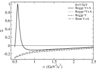
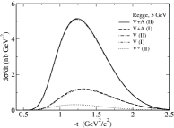
$(a)$                                               $(b)$                                               $(c)$

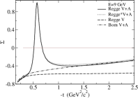
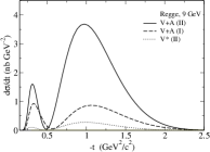
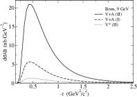
Figure 2: The $p\bar{p}$ photoproduction off the proton, $E_{\gamma}=\,$5 GeV: ($a$) beam asymmetry $\Sigma_{p\bar{p}}$, ($b$) $d\sigma_{p\bar{p}}/dt$ in the Regge-pole approximation, ($c$) $d\sigma_{p\bar{p}}/dt$ in the Born approximation. In panel $a$, the lower two curves (without a peak at $-t\approx\,$0.6 GeV²) correspond to the vector meson exchange ($V=\rho+\omega$) in the Born (dotted-dashed curve) and Regge-pole (dashed curve) approximations. The upper two curves are obtained for the sum of vector and axial-vector meson exchanges ($V+A=\rho+\omega+b_{1}+h_{1}$) for the Regge-pole approximation with taking into account six (solid curve) and three (pointed curve) intermediate scalar mesons, respectively. In panel $b$, results for two sets of effective parameters are presented: the lower two curves – variant I (dashed for $V+A$ and two-pointed dashed for $V$ exchanges) and the upper two curves, variant II (solid for $V+A$ and dotted-dashed for $V$ exchanges). In panel $c$, the same notations for the curves are used as in panel $b$. Dotted curves in panels $a$, $b$, and $c$ show the results obtained with taking into account the contribution of only three intermediate scalar mesons, $f_{0}(1370)$, $f_{0}(1500)$, and $f_{0}(1710)$. The rest takes into account also the contribution of $f_{0}(2020)$, $f_{0}(2100)$, and $f_{0}(2200)$.

$(a)$                                               $(b)$                                               $(c)$

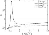
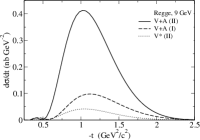
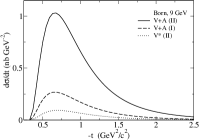
Figure 3: The $p\bar{p}$ photoproduction for $E_{\gamma}=\,$9 GeV. The same content of panels as in Fig. 5.

$(a)$                                               $(b)$                                               $(c)$

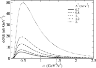
Figure 4: The $\Lambda\bar{\Lambda}$ photoproduction for $E_{\gamma}=\,$9 GeV. The same content of panels as in Fig. 5.

Figure 5: The $p\bar{p}$ photoproduction for $E_{\gamma}=\,$9 GeV. The Born approximation for different values of the cutoff parameters $\Lambda=\Lambda_{V}=\Lambda_{A}$ ($\Lambda^{2}=\,$0.8, 1, 1.2, and 2 GeV²) is shown in comparison to the choice $\Lambda^{2}=\,$0.7 GeV² (solid curve) used in this work.

References

(1)
H. Al Ghoul et al. (GlueX Collaboration),
Phys. Rev. C 95, 042201(R) (2017).
(2)
J. M. Laget
Phys. Lett. B 695, 199 (2011).
(3)
V. Mathieu, G. Fox, and A. P. Szczepaniak,
Phys. Rev. D 92, 074013 (2015).
(4)
J. Nys, et al. (JPAC Collaboration),
Phys. Rev. D 95, 034014 (2017).
(5)
A. Donnachie and Yu. S. Kalashnikova,
Phys. Rev. C 93, 025203 (2016).
(6)
F. Giacosa, T. Gutsche, V. E. Lyubovitskij, and A. Faessler,
Phys. Lett. B 622, 277 (2005).
(7)
P. Chatzis, A. Faessler, T. Gutsche, and V. E. Lyubovitskij,
Phys. Rev. D 84, 034027 (2011).
(8)
T. Gutsche, S. Kuleshov, V.E. Lyubovitskij, and I.T. Obukhovsky,
Phys. Rev. D 94, 034010 (2016).
(9)
C. Patrignani et al.
(Particle Data Group Collaboration), Chin. Phys. C 40, 100001 (2016).
(10)
V.A. Matveev, R.M. Muradian, and A.N. Tavkhelidze,
Lett. Nuovo Cimento 7, 719 (1973).
(11)
S.J. Brodsky and G.R. Farrar,
Phys. Rev. Lett. 31, 1153 (1973).
(12)
G.P. Lepage and S.J. Brodsky,
Phys. Rev. D 22, 2157 (1980).
(13)
L. P. Gamberg and G. R. Goldstein,
Phys. Rev. Lett. 87, 242001 (2001).
(14)
M. Guidal, J.-M. Laget, and M. Vanderhaeghen,
Nucl. Phys. A 627, 645 (1997).
(15)
R. Machleidt,
Phys. Rev. C 63, 024001 (2001).