Technical Report
Millimeter Wave Communication in Vehicular Networks: Coverage and Connectivity Analysis

In this technical report (TR), we will report the mathematical model we developed to carry out the preliminary coverage and connectivity analysis in mmWave-based vehicular networks, proposed in our work [1]. The purpose is to exemplify some of the complex and interesting tradeoffs that have to be considered when designing solutions for mmWave automotive scenarios.

The rest of TR is organized as follows. In Section 1, we describe the scenario used to carry out our simulation results, presenting the main setting parameters and the implemented mmWave channel model. In Section 2 we report the mathematical model used to develop our connectivity and coverage analysis. Finally, in Section 3, we show our main findings in terms of throughput.

1   Simulation Settings

We consider a simple but representative V2I scenario, where a single Automotive Node (AN, i.e., a car) moves along a road at constant speed $V$ and Infrastructure Nodes (INs, i.e., static mmWave Base Stations) are randomly distributed according to a Poisson Point Process (PPP) of parameter $\rho$ nodes/km, so that the distance $d$ between consecutive nodes is an exponential random variable of mean $\mathbb{E}[d]=1/\rho$ km (see, e.g., [2]).

1.1 Millimeter Wave Channel Model

As assessed in [1], in order to overcome the increased isotropic path loss experienced at higher frequencies, next-generation mmWave automotive communication must provide mechanisms by which the vehicles and the infrastructures determine suitable directions of transmission for spreading around their sensors information, thus exploiting beamforming (BF) gain at both the transmitter and the receiver side. To provide a realistic assessment of mmWave micro and picocellular networks in a dense urban deployment, we considered the channel model obtained from recent real-world measurements at $28$ GHz in New York City. Further details on the channel model and its parameters can be found in [3].

The link budget for the mmWave propagation channel is defined as:

$$P_{RX}=P_{TX}+G_{BF}-PL-\xi$$ (1)

where $P_{RX}$ is the total received power expressed in dBm, $P_{TX}$ is the transmit power, $G_{BF}$ is the gain obtained using BF techniques, $PL$ represents the pathloss in dB and ${\xi\sim N(0,\sigma^{2})}$ is the shadowing in dB, whose parameter $\sigma^{2}$ comes from the measurements in [3].

Based on the real-environment measurements of [3], the pathloss can be modeled through three different states: Line-of-Sight (LoS), Non-Line-Of-Sight (NLoS) and outage. Based on the distance $d$ between the transmitter and the receiver, the probability to be in one of the states ($P_{\text{LoS}}$, $P_{\text{NLoS}}$, $P_{\text{out}}$) is computed by:

$$\begin{split}P_{\text{out}}(d)&=\max(0,1-e^{-a_{\text{out}}d+b_{\text{out}}})\\ P_{\text{LoS}}(d)&=(1-P_{\text{out}}(d))e^{-a_{\text{LoS}}d}\\ P_{\text{NLoS}}(d)&=1-P_{\text{out}}(d)-P_{\text{LoS}}(d)\end{split}$$ (2)

where parameters ${a_{\text{out}}=0.0334}$ m^-1, ${b_{\text{out}}=5.2}$ and ${a_{\text{LoS}}=0.0149}$ m^-1 have been obtained in [3] for a carrier frequency of $28$ GHz. The pathloss is finally obtained by:

$$PL(d)[dB]=\alpha+\beta 10\log_{10}(d)$$ (3)

where $d$ is the distance between receiver and transmitter, and the value of the parameters $\alpha$ and $\beta$ are given in [3].

To generate random realizations of the large-scale parameters, the mmWave channel is defined as a combination of a random number $K\sim\max\{\text{Poisson}(\lambda),1\}$ of path clusters, for which the parameter $\lambda$ can be found in [3], each corresponding to a macro-level scattering path. Each cluster is further composed of several subpaths $L_{k}\sim U[1,10]$.

The time-varying channel matrix is described as follows:

$$\textbf{H}(t,f)=\frac{1}{\sqrt{L}}\sum_{k=1}^{K}\sum_{l=1}^{L_{k}}g_{kl}(t,f)\textbf{u}_{rx}(\theta_{kl}^{rx},\phi_{kl}^{rx})\textbf{u}^{*}_{tx}(\theta_{kl}^{tx},\phi_{kl}^{tx})$$ (4)

where $g_{kl}(t,f)$ refers to the small-scale fading over time and frequency on the $l^{\text{th}}$ subpath of the $k^{\text{th}}$ cluster and $\textbf{u}_{rx}(\cdot)$, $\textbf{u}_{tx}(\cdot)$ are the spatial signatures for the receiver and transmitter antenna arrays and are functions of the central azimuth (horizontal) and elevation (vertical) Angle of Arrival (AoA) and Angle of Departure (AoD), respectively $\theta_{kl}^{rx}$, $\phi_{kl}^{rx}$, $\theta_{kl}^{tx}$, $\phi_{kl}^{tx}$ .

The small-scale fading in Equation (4) describes the rapid fluctuations of the amplitude of a radio signal over a short period of time or travel distance. It is generated based on the number of clusters, the number of subpaths in each cluster, the Doppler shift, the power spread, and the delay spread, as:

$$g_{kl}(t,f)=\sqrt{P_{lk}}e^{2\pi if_{d}\cos(\omega_{kl})t-2\pi i\tau_{kl}f},$$ (5)

where:

• $P_{lk}$ is the power spread of subpath $l$ in cluster $k$, as defined in [3];

• $f_{d}$ is the maximum Doppler shift and is related to the user speed ($v$) and to the carrier frequency $f$ as $f_{d}=fv/c$, where $c$ is the speed of light;

• $\omega_{kl}$ is the angle of arrival of subpath $l$ in cluster $k$ with respect to the direction of motion;

• $\tau_{kl}$ gives the delay spread of subpath $l$ in cluster $k$;

• $f$ is the carrier frequency.

Due to the high pathloss experienced at mmWaves, multiple antenna elements with beamforming are essential to provide an acceptable communication range. The BF gain parameter in (1) from transmitter $i$ to receiver $j$ is thus given by:

$$G_{BF}(t,f)_{ij}=|\textbf{w}^{*}_{rx_{ij}}\textbf{H}(t,f)_{ij}\textbf{w}_{tx_{ij}}|^{2}$$ (6)

where $\textbf{H}(t,f)_{ij}$ is the channel matrix of the $ij^{th}$ link, $\textbf{w}_{tx_{ij}}\in\mathbb{C}^{n_{\mathbb{T}x}}$ is the BF vector of transmitter $i$ when transmitting to receiver $j$, and $\textbf{w}_{rx_{ij}}\in\mathbb{C}^{n_{\mathbb{R}x}}$ is the BF vector of receiver $j$ when receiving from transmitter $i$. Both vectors are complex, with length equal to the number of antenna elements in the array, and are chosen according to the specific direction that links BS and UE.

The channel quality is measured in terms of Signal-to-Interference-plus-Noise-Ratio (SINR). By referring to the mmWave statistical channel described above, the SINR between a transmitted $\rm j$ and a test RX can computed in the following way:

$$\Gamma=\text{SINR}_{\rm j,RX}=\frac{\frac{P_{\rm TX}}{PL_{\rm j,UE}}G_{\rm j,RX}}{\sum_{\rm k\neq j}\frac{P_{\rm TX}}{PL_{\rm k,RX}}G_{\rm k,RX}+W_{\rm tot}\times N_{0}}$$ (7)

where $G_{\rm i,RX}$ and $PL_{\rm i,RX}$ are the BF gain and the pathloss obtained between transmitter $i$ and the test RX, respectively, and $W_{\rm tot}\times N_{0}$ is the thermal noise.

1.2 System Model

We say that an AN is within coverage $(R_{\rm comm})$ of a certain IN if, assuming perfect beam alignment, the SINR is the best possible for the AN, and it exceeds a minimum threshold, which we set to $\Gamma_{0}=-5$ dB. Due to the stochastic nature of the signal propagation and of the interference, the coverage range of an IN is a random variable, whose exact characterization is still unknown but clearly depends on a number of factors, such as beamwidth, propagation environment, and level of interference that, in turn, depends on the spatial density of the nodes.

To gain some insights on these complex relationships, we performed a number of simulations and evaluated the mean coverage range $R_{\rm comm}$ when varying the node density and the antenna configuration of the nodes. Tab. 1 collects the main simulation parameters, which are based on realistic system design considerations. A set of two dimensional antenna arrays is used at both the INs and the ANs. INs are equipped with a Uniform Planar Array (UPA) of $2\times 2$ or $8\times 8$ elements, while the ANs exploit an array of $2\times 2$ or $4\times 4$ antennas. The spacing of the elements is set to $\lambda/2$, where $\lambda$ is the wavelength. In general, as depicted in Fig. 1, $R_{\rm comm}$ increases with the number of antennas, thanks to the narrower beams that can be realized, which increase the beamforming gain. On the other hand, $R_{\rm comm}$ decreases as the density of nodes increases, because of the larger amount of interference received at the AN from the INs due to their reduced distance.

Parameter	Value	Description
$W_{\rm tot}$	$1$ GHz	Total system bandwidth
DL $P_{\rm TX}$	$30$ dBm	Transmission power
NF	$5$ dB	Noise figure
$f_{\rm c}$	$28$ GHz	Carrier frequency
$\tau$	$-5$ dB	Minimum SINR threshold
$N_{\rm BS}$	{4, 64}	BS MIMO array size
$N_{\rm veh}$	{4, 16}	Vehicular MIMO array size
$T_{\rm RTO}$	{0.025, 0.1, 0.2, 0.5, 1} s	Slot duration
$V$	{10, 20, 30, 100, 130} km/h	Vehicle speed
$R_{\rm comm}$	Varied	Communication radius

Table 1: Main simulation parameters.

Figure 1: Average coverage range $R_{\rm comm}$ (for different MIMO configurations) versus the nodes density $\rho$.

As we pointed out in [1], a directional beam pair needs to be determined to enable the transmission between two ANs, thus beam tracking heavily affects the connectivity performance of a V2X mmWave scenario. In this analysis, according to the procedure described in [4, 5], we assume that measurement reports are periodically exchanged among the nodes so that, at the beginning of every slot of duration $T_{\rm RTO}$, ANs and INs identify the best directions for their respective beams. Such configuration is kept fixed for the whole slot duration, during which nodes may lose the alignment due to the AN mobility. In case the connectivity is lost during a slot, it can only be recovered at the beginning of the subsequent slot, when the beam tracking procedure is performed again. It is hence of interest to evaluate the AN connectivity, i.e., the fraction of slots in which the AN and the IN remain connected (since the AN is in the IN’s coverage range), as a function of the following parameters: (i) the MIMO configuration; (ii) the vehicle speed $V$; (iii) the slot duration $T_{\rm RTO}$; (iv) the node density $\rho$.

At the beginning of a time slot, the AN can be either in a connected (C) state, if it is within the coverage range of an IN, or in an idle (I) state, if there are no INs within a distance $R_{\rm comm}$. Starting from state C, the AN can either maintain connectivity to the serving IN for the whole slot duration, or lose the beam alignment and get disconnected. Starting from state I, instead, the AN can either remain out-of-range for the whole slot of duration $T_{\rm RTO}$, or enter the coverage range of a new IN within $T_{\rm RTO}$ (catch-up). Even in this second case, however, the connection to the IN will be established only at the beginning of the following slot, when the beam alignment procedure will be performed. Therefore, preservation of the connectivity during a slot requires that the AN is within the coverage range of the IN at the beginning of the slot and does not lose beam alignment in the slot period $T_{\rm RTO}$. In this case, the vehicle can potentially send data with a rate $R(d)$ that depends on the distance $d$ to the serving IN.

2   Coverage and Connectivity Analysis

In order to determine the average throughput a vehicular node will experience in the considered simple automotive scenario, as a function of several V2X parameters, we first need to compute the average portion of slot in which the VN is both within the coverage of an infrastructure node and properly aligned. To do so, in this section we will: (i) evaluate the probability for the VN to be within $R_{\rm comm}$, at the beginning of the slot; (ii) evaluate the probability for the VN not to misalign within the slot; (iii) finally evaluate the mean communication duration.

2.1 Probability of Starting the Communication

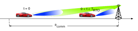
Figure 2: Scenario in which the VN is both within the coverage range $R_{\rm comm}$ of its serving IN and properly aligned for the whole slot of duration $T_{\rm RTO}$.

The communication can start, within the slot of duration $T_{\rm RTO}$, only if the vehicle is already within the coverage range $R_{\rm comm}$, with probability $\mathbb{P}_{D}(R_{\rm comm})$:

$$P_{\rm start}=\mathbb{P}[d\leq 2R_{\rm comm}]=1-e^{-2\rho R_{\rm comm}}$$ (8)

Figure 3: Probability of starting the communication vs. nodes density $\rho$, when VN moves at constant speed $V=90$ km/s and $T_{\rm RTO}=200$ ms.

From the results in Figure 3, we deduce that:

• $P_{\rm start}$ increases with the IN density $\rho$, since the mean distance $\mathbb{E}[d]=1/\rho$ from the IN decreases, so it’s more likely for the AN to fall within the coverage range of the IN. On the other hand, although the communication range $R_{\rm comm}$ is reduced when considering denser networks, due to the increased interference perceived by the vehicular node, $P_{\rm start}$ still increases, making the reduction of the distance dominant to the increased interference.

• $P_{\rm start}$ increases when increasing the MIMO order, that is when packing more antenna elements in the MIMO array. In fact, keeping $\rho$ fixed, beams are narrower, interference is reduced, the achieved BF gain is higher, and the increased $R_{\rm comm}$ makes the discoverable range of the IN increased as well.

2.2 Probability of NOT Leaving the Communication

Constraining on the probability of having started the communication within the slot of duration $T_{\rm RTO}$ , the vehicle loses its ability to communicate with the IN with probability $1-P_{\rm NL}$, where $P_{\rm NL}$ is defined as:

$$P_{\rm NL}=P_{\rm start}\cdot\mathbb{P}(T_{\rm L}>T_{\rm RTO}).$$ (9)

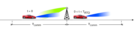
Figure 4: At the beginning of the slot, the AN is connected to the IN, steering the beam to an angle of 0^∘. When moving at constant speed $V$ during the slot, the AN overtakes the IN (now on its left). Since the beam direction cannot be updated during the slot, the link between the AN and IN will be lost till the beginning of the next slot.

If the vehicle was already in the communication range at the beginning of the slot, it does not leave the communication with probability $\mathbb{P}(T_{\rm L}>T_{\rm RTO})$, that is if it covers a distance smaller than $d|d<R_{\rm comm}$, within $T_{\rm RTO}$, moving at relative speed $V>0$:

$$\mathbb{P}(T_{\rm L}>T_{\rm RTO})=$$ (10)

$$=1-\mathbb{P}(\text{Overtaking the IN within }T_{\rm RTO}|\text{vehicle is connected})=$$

$$=\mathbb{P}\Big{[}\dfrac{d}{V}>T_{\rm RTO}|d<R_{\rm comm}\Big{]}=\frac{e^{-\rho T_{\rm RTO}V}-e^{-\rho R_{\rm comm}}}{1-e^{-\rho R_{\rm comm}}}$$

On the other hand, if the AN overtakes the IN (as in Figure 4) during the slot, although theoretically being under the coverage of the infrastructure, it needs to adapt its beam orientation to be perfectly aligned; however, this operation can be triggered only at the beginning of the subsequent slot, making the AN misaligned and thus disconnected for the whole remaining slot period.

(a) $P_{\rm NL}$ with $V=90$ km/s and $T_{\rm RTO}=200$ ms, for different MIMO configurations.

(b) $P_{\rm NL}$ with $T_{\rm RTO}=200$ ms and MIMO configuration $64\times 16$, for different speeds.

(c) $P_{\rm NL}$ with $V=90$ km/h and MIMO configuration $64\times 16$, for different slot durations.

Figure 5: Probability of not leaving the communication ($P_{\rm NL}$) within a time slot of duration $T_{\rm RTO}$ when varying the nodes spatial density $\rho$.

In Figure 5, we plot the probability of not leaving the communication ($P_{\rm NL}$) and we state that:

• $P_{\rm NL}$ increases with $\rho$, for sparse networks ($\rho$ small). On one hand, $P_{\rm start}$ increases but, on the other hand, the AN is closer and closer to the IN (the mean distance $\mathbb{E}[d]=1/\rho$ from the IN decreases) and, within the same time slot $T_{\rm RTO}$, it is more and more likely for the AN to overtake the IN and being misaligned. However, when the infrastructure nodes are quite scattered, the mean distance $\mathbb{E}[d]=1/\rho$ is relatively large and so the increasing behavior of $P_{\rm start}$ in Eq. (9) is dominant.

• $P_{\rm NL}$ decreases with increasing values of $\rho$, for dense networks ($\rho$ large). In fact, $P_{\rm start}$ has reached a quasi-steady state (see Figure 3) and almost does not increase as $\rho$ increases, whereas the mean distance $\mathbb{E}[d]=1/\rho$ keeps reducing, thus increasing the chances for the AN to leave its serving IN’s connectivity range and be misaligned.

• $P_{\rm NL}$ increases when $V$ decreases since, when the VN is slower, it has less chances to leave the communication range of the IN within the same time slot of duration $T_{\rm RTO}$.

• $P_{\rm NL}$ increases when $T_{\rm RTO}$ decreases, since the AN covers a shorter distance $V\cdot T_{\rm RTO}$ moving at the same speed $V$, thus reducing the chances to leave its serving IN’s communication range.

2.3 Mean Communication Duration

The communication is "active" only when the vehicle is both within the coverage range of the IN and correctly aligned, during the slot of duration $T_{\rm RTO}$. Constraining on the probability of having started the communication, the mean communication duration is:

$$\mathbb{E}[T_{\rm comm}]=P_{\rm start}\cdot\Big{[}\mathbb{P}(T_{\rm L}>T_{\rm RTO})T_{\rm RTO}\>+\>\Big{(}1-\mathbb{P}(T_{\rm L}>T_{\rm RTO})\Big{)}\mathbb{E}[T_{\rm L}]\Big{]}.$$ (11)

In particular, if the vehicle was already in the communication range at the beginning of the slot:

1. if the vehicle never overtakes its serving IN and never becomes misaligned within the slot (with probability $\mathbb{P}(T_{\rm L}>T_{\rm RTO})$), it communicates for the whole slot, so for a duration $T_{\rm RTO}$;

2. if, at some point, the vehicle becomes misaligned with its IN, although being inside $R_{\rm comm}$ during the slot (with probability $1-\mathbb{P}(T_{\rm L}>T_{\rm RTO})$), it communicates only for the time $\mathbb{E}[T_{\rm L}]<T_{\rm RTO}$ in which it was correctly able to be served (during this time window, the VN has covered a distance $d|d<T_{\rm RTO}V$, moving at speed $V$), where:

   $$\mathbb{E}[T_{\rm L}]=$$ (12)

   $$=\mathbb{E}[\text{Time in which the VN is aligned within }R_{\rm comm}|\text{VN is connected but leaves }]=$$

   $$=\dfrac{\mathbb{E}[{d|d<T_{\rm RTO}V|d<R_{\rm comm}}]}{V}=$$

   $$=\frac{1}{V}\frac{1}{\mathbb{P}[d<T_{\rm RTO}V|d<R_{\rm comm}]}\int_{0}^{T_{\rm RTO}V}\eta p_{d}(\eta)d\eta\overset{(a)}{=}$$ (13)

   $$=\frac{1}{V}\frac{1-e^{-\rho R_{\rm comm}}}{1-e^{-\rho T_{\rm RTO}V}}\frac{1-e^{-\rho T_{\rm RTO}V}(\rho T_{\rm RTO}V+1)}{\rho},$$

where step $(a)$ is based on the fact that, in realistic vehicular environments, $T_{\rm RTO}V\ll R_{\rm comm}$. In Figure 6, we plot the communication duration ratio, that is the ratio between the portion of time slot in which the VN is both within the communication range $R_{\rm comm}$ of its serving IN and properly aligned ($\mathbb{E}[T_{\rm comm}]$) and the whole slot duration ($T_{\rm RTO}$) (i.e., $\mathbb{E}[T_{\rm comm}]/T_{\rm RTO}=1$ if the VN is connected for the whole time slot). We observe that results agree with the considerations we made in the previous subsection and, in particular:

(a) $\mathbb{E}[T_{\rm L}]/T_{\rm RTO}$ with $V=90$ km/s and $T_{\rm RTO}=200$ ms, for different MIMO configurations.

(b) $\mathbb{E}[T_{\rm L}]/T_{\rm RTO}$ with $T_{\rm RTO}=200$ ms and MIMO configuration $64\times 16$, for different speeds.

(c) $\mathbb{E}[T_{\rm L}]/T_{\rm RTO}$ with $V=90$ km/h and MIMO configuration $64\times 16$, for different slot durations.

Figure 6: Portion of time slot (of duration $T_{\rm RTO}$) in which the VN is both within the communication range $R_{\rm comm}$ of its serving IN and properly aligned, when varying the nodes spatial density $\rho$.

• $\mathbb{E}[T_{\rm comm}]/T_{\rm RTO}$ increases with $\rho$, for sparse networks ($\rho$ small), since the mean distance $\mathbb{E}[d]=1/\rho$ is relatively large and it is very unlikely for the AN to overtake its serving IN and become misaligned. The increasing behavior of the communication duration ratio is therefore caused by the increased probability of being within $R_{\rm comm}$ at the beginning of the slot.

• $\mathbb{E}[T_{\rm comm}]/T_{\rm RTO}$ decreases with increasing values of$\rho$, for dense networks ($\rho$ large). In fact $P_{\rm start}$ has reached a quasi-steady state (see Figure 3) and almost does not increase as $\rho$ increases, while the mean distance $\mathbb{E}[d]=1/\rho$ keeps reducing, thus increasing the chances for the AN to overtake the IN and disconnect.

• $\mathbb{E}[T_{\rm comm}]/T_{\rm RTO}$ increases for lower values of $V$ and $T_{\rm RTO}$. Therefore, we assess that considering slower vehicular nodes or updating more frequently the AN-IN beam pair, respectively, reflects an increased average communication duration.

3   Throughput Analysis

(a) Throughput with $V=90$ km/s and $T_{\rm RTO}=200$ ms, for different MIMO configurations.

(b) Throughput with $T_{\rm RTO}=200$ ms and MIMO configuration $64\times 16$, for different speeds.

(c) Throughput with $V=90$ km/h and MIMO configuration $64\times 16$, for different slot durations.

Figure 7: Average throughput within a time slot of duration $T_{\rm RTO}$ when varying the nodes spatial density $\rho$.

A non-zero throughput can be perceived (within the slot of duration $T_{\rm RTO}$) only when the vehicle is within coverage and properly aligned with the infrastructure, that is for a time $\mathbb{E}[T_{\rm comm}]$. In this period, the vehicle perceives a rate $\mathbb{E}[R(d)]$ that depends on the mean distance $\mathbb{E}[d]=1/\rho$, proportional to the nodes spatial density $\rho$. The throughput is therefore defined as:

$$B=\mathbb{E}[R(d)]\cdot\frac{\mathbb{E}[T_{\rm comm}]}{T_{\rm RTO}}$$ (14)

In Figure 7 and 8, we report the average throughput, when varying some system parameters. It is rather interesting to observe that, in all considered configurations, the throughput exhibits a similar pattern when varying the node density $\rho$. In particular:

Figure 8: Average throughput perceived by a vehicular node, considering a node spatial density $\rho=20$ nodes/km and $T_{\rm RTO}=200$ ms, for different MIMO configurations and for different speed values $V$.

• We note that, as the node density is increased, the average distance between the AN and the IN decreases and, hence, the average bit rate experienced by the AN in case of connectivity becomes larger. On the other hand, the smaller coverage range will increase the probability of losing connectivity during a slot and will determine an increment of the frequency of handovers.

• For small values of $\rho$, $B$ initially increases with $\rho$. In this region, the SINR increases with $\rho$ because the reduction of the mean distance to the serving IN is more significant than the increase of the interference coming from the neighboring INs. Moreover, the distance between adjacent INs is still sufficiently large to allow for a loose beam alignment (thanks to the widening of the beam with the distance), so that the connectivity between the AN and the IN is maintained for a relatively large number of slots.

• After a certain value of $\rho$ (approximately 40 nodes/km in our scenario), $B$ starts decreasing. In this region, the interference from close-by INs becomes dominant and the perceived SINR degrades. Moreover, the closer the distance between the IN and the AN, the smaller the beam widening and, hence, the higher the risk of losing connectivity during a slot.

• the throughput grows as $V$ decreases since a slower AN is less likely to lose connectivity to the serving IN during a slot.

• Similarly, the throughput grows as $T_{\rm RTO}$ decreases, because the beam alignment is repeated more frequently, reducing the disconnection time. However, the overhead (which is not accounted for in this simple analysis) would also increase, thus limiting or even nullifying the gain.

• Finally, as shown in Figure 1, the throughput grows with the MIMO array size due to the increased achievable communication range $R_{\rm comm}$ of the nodes.

In conclusion, we have presented a preliminary connectivity and coverage study in a simple automotive scenario using mmWave communication link, and show how the performance of common directional beam tracking protocols can be improved by accounting for the specificities of the automotive scenario.

References

- [1] M. Giordani, A. Zanella, and M. Zorzi, “Millimeter wave communication in vehicular networks: Challenges and opportunities,” accepted to International Conference on Modern Circuits and Systems Technologies (MOCAST), 2017.
- [2] W. Leutzbach, Introduction to the theory of traffic flow. Springer, 1988, vol. 47.
- [3] M. R. Akdeniz, Y. Liu, M. K. Samimi, S. Sun, S. Rangan, T. S. Rappaport, and E. Erkip, “Millimeter wave channel modeling and cellular capacity evaluation,” IEEE Journal on Selected Areas in Communications, vol. 32, no. 6, pp. 1164–1179, June 2014.
- [4] M. Giordani, M. Mezzavilla, S. Rangan, and M. Zorzi, “Uplink-based framework for control plane applications in 5G mmWave cellular networks,” arXiv preprint arXiv:1610.04836, 2016.
- [5] ——, “Multi-Connectivity in 5G mmWave cellular networks,” in 15th Annual Mediterranean Ad Hoc Networking Workshop (Med-Hoc-Net’16), Jun. 2016.