2D simulation of helical flux compression generator

Abstract

Diverse approaches to HFCG’s inductance,resistance and armature expansion calculating are evaluated. Comparison of simulated and experimentally obtained results is provided. Validity criteria for different simulation models are proposed. Consideration of armature acceleration under the pressure of detonation products is shown to be beneficial for accuracy of HFCG simulation. Control of HFCG temperature during simulation enables detecting critical points of system operation.

I Introduction

Helical flux-compression generators (HFCG) are the useful compact power sources. Being easily varied by size, shape, coil pitch and means for initial flux creation, HFCG could be used for various high-energy and high-current pulsed power applications. Development of high-performance generators requires accurate modelling of HFCGs operation by the use of a 2D or even a 3D approach [1, 2, 3, 4] and consideration of multiple factors [5, 6] affecting HFCG gain, efficiency and output parameters. Some of theses factors (like 2-pi clocking, crowbar losses, electrical breakdown etc.) should be apprehended and avoided by HFCG proper design and manufacturing. Unavoidable effects like inter-turn proximity effect in the helical coil, diffusion losses in the vicinity of the contact point between armature and stator, magnetic field pressure affecting the expanding armature motion, high-temperature effects and etc. should be taken into account as thoroughly as possible [7].

With the goal to demonstrate ranges of validity and propose validity criteria for diverse approaches to HFCG simulation a modular code FCGcalc was developed. HFCG simulation by this code is presented in the paper. FCGcalc allows selecting multiple options. One- or two-dimensional model can be used for inductance calculation (”1D” or ”2D” options) [10, 1]. Two approaches are available to describe armature expansion: the armature expanding part is either considered to be a cone, which angle is equal to the armature expansion angle (armature velocity) defined by Gurney equation [8], or calculated by equations of a hollow tube motion under the pressure of detonation products according to [6, 9] (”Gurney” or ”pressure” options). Consideration of all nonlinear effects (nonlinear diffusion, magnetic field pressure) can be turned off to reveal their influence on FCG operation (”linear” or ”nonlinear” options).

Fast high-power HFCGs with moderate parameters loaded by a mostly inductive load were analyzed with the view of ensuring the predictive power for performance of the developed HFCG. The set of specially designed HFCGs were tested in conditions when the most of factors those could be scarcely considered in simulation were either avoided or additionally controlled. The present paper includes simulation approach and results, comparison of simulated and experimentally obtained results with the very brief description of HFCG experimental testing.

II Basic Physics

The equation for the performance of ”HFCG+inductive load” circuit is given with Kirchhof’s voltage law by [6, 10, 11]:

$$\left({L_{g}+L_{l}}\right)\dot{I}+\left({\frac{{dL_{g}}}{{dt}}+R_{g}}\right)I=0,$$ (1)

where ”dot” means time derivative, $R_{g}$ is the HFCG resistance including losses of all types, $L_{g}$ and $L_{l}$ are inductances of HFCG and the load, respectively. Evaluation of time-dependant $R_{g}$ and $L_{g}$, which are neither dc no ac resistance and inductance of HFCG, requires consideration of both mechanical and electrodynamic aspects. Difficulty is caused by the complicated geometry of HFCG inner volume closed between coil (which usually is tapered in diameter and has multi-sectional winding) and expanding armature as well as by the nonlinear diffusion of magnetic field into HFCG conductors in conditions, when the current carrying layers on the armature surface are not fixed.

One-dimensional model for inductance calculation is considered in [10], where the HFCG inductance per unit length reads as follows:

$$\frac{{dL_{g}}}{{dz}}=\pi\mu_{0}n^{2}\left({R_{S}^{2}-R_{A}^{2}}\right)+\frac{{\mu_{0}}}{{2\pi}}ln\frac{{R_{S}}}{{R_{A}}},$$ (2)

where $n$ is the winding density, the stator radius $R_{S}$ and armature radius $R_{A}$ are both functions of z, while $R_{A}$ is also time-dependant.

According to 2D approach [1] the total HFCG inductance is presented as a sum of axial $L_{z}$ and azimuth $L_{\theta}$ components due to axial and azimuth currents in HFCG circuit: $L_{g}=L_{\theta}+L_{z}$. Contribution due to axial current can be derived from [6, 10]:

$$\frac{{dL_{z}}}{{dz}}=\frac{{\mu_{0}}}{{2\pi}}ln\frac{{R_{S}}}{{R_{A}}},$$

The effective approach to calculation of HFCG inductance $L_{\theta}$ due to azimuth currents was proposed by [1] and considered in details in [6]. This approach implies approximation of HFCG conductors by a set of single-turn cylindrical sheet perfectly conducting solenoids (rings) of infinitesimal width $\Delta z\to 0$, each carrying a uniform current. Rings radii $R_{i}$ are defined as the inner radius of stator at $z_{i}$ for stator rings and outer radius of expanding armature at $z_{i}$ for armature rings (expressions describing expanding armature radius see therein below). The inductance $L_{\theta}$ can be found from the equality

$$\frac{{1}}{{2}}\sum M_{ij}I_{i}I_{j}=\frac{{L_{\theta}I^{2}}}{{2}},$$ (3)

where $I_{i}$ is the current over $i$-th ring, $M_{ii}$ is the inductance of the $i$-th ring and $M_{ij}$ is the mutual inductance of two rings with centers distant $x_{ij}$,

$$M_{ii}=\mu_{0}R_{i}\left({ln\frac{{16R_{i}}}{{\Delta z}}-2}\right),$$ (4)

$$M_{ij}=\mu_{0}\left(\frac{{R_{i}^{2}+R_{j}^{2}+x_{ij}^{2}}}{{\sqrt{\left({R_{i}+R_{j}}\right)^{2}+x_{ij}^{2}}}}K\left({\frac{{4R_{i}R_{j}}}{{\left({R_{i}+R_{j}}\right)^{2}+x_{ij}^{2}}}}\right)\right)$$

$$-\mu_{0}\left(\sqrt{\left({R_{i}+R_{j}}\right)^{2}+x_{ij}^{2}}E\left({\frac{{4R_{i}R_{j}}}{{\left({R_{i}+R_{j}}\right)^{2}+x_{ij}^{2}}}}\right)\right),$$

where

$$K=\int^{\pi/2}_{0}(1-k^{2}\sin^{2}\theta)^{-1/2}d\theta$$

and

$$E=\int^{\pi/2}_{0}(1-k^{2}\sin^{2}\theta)^{1/2}d\theta$$

are the complete elliptic integrals of the first and second kind, $k=\sqrt{{\textstyle{{4R_{i}R_{j}}\over{\left({R_{i}+R_{j}}\right)^{2}+x_{ij}^{2}}}}}$ [12, 11]. Condition $\sum M_{ij}I_{j}=0$ is valid for perfect conducting stator and armature. Azimuth current $I_{i}=n\left({z_{i}}\right)\Delta zI$ over a stator ring located at axial coordinate $z_{i}$ is fixed by the circuit total current $I$ and the winding density $n=n\left({z}\right)$:

$$n\left({z=z_{i}}\right)=\frac{{\sqrt{\left({2\pi R_{i}/n_{t}}\right)^{2}-\left({d_{w}+2\Delta_{w}}\right)^{2}}}}{{2\pi R_{i}\left({d_{w}+2\Delta_{w}}\right)}},$$ (5)

where $R_{i}=R_{S}\left({z_{i}}\right)$ and the stator radius $R_{S}$, the winding wire diameter $d_{w}$, the isolation thickness $\Delta_{w}$ and the number of winding turns $n_{t}$, all are the functions of $z$. Azimuth currents over the armature are conditioned by the stator azimuth currents as follows:

$$I_{A}=-M_{AA}^{-1}M_{AS}I_{S},$$

where $I_{A}$, is the column vector describing currents over armature rings, $I_{S}$ is the same for the stator currents, $M_{AA}$ is the matrix of self and mutual inductances of armature rings, $M_{AS}$ is the matrix of mutual inductances of armature and stator rings. The armature expanding part is either considered to be a cone, which angle is equal to the armature expansion angle defined by Gurney equation [8], or calculated by equations of a hollow tube motion under the pressure of detonation products according to [9, 6]. In the latter case armature rings radii at the axial coordinate $z_{i}$ at the instant $t_{i}$ are defined by:

$$R_{i}=\sqrt{r_{i}^{2}+R_{0}^{2}-r_{0}^{2}},$$ (6)

$$\ddot{r}_{i}=2\pi\frac{r_{i}\left(\frac{p_{H}}{2}\left(\frac{r_{0i}}{r_{i}}\right)^{2k}-\frac{R_{i}-r_{i}}{r_{i}}\sigma_{D}\right)-\rho_{A}\dot{r}_{i}^{2}\left(\frac{R_{i}^{2}+r_{i}^{2}}{R_{i}}-2r_{i}\right)}{m/2+2\pi\rho_{A}r_{i}\left({R_{i}-r_{i}}\right)},$$

$$r_{i}\left({t_{i}}\right)=r_{0},\,\,\,\,\frac{d{r}_{i}}{dt}\left({t_{i}}\right)=0,$$

where $\sigma_{D}$ is the dynamic yield strength, $k$ is the isentrope index for detonation products, $t_{i}$ is the instant, when detonation front comes to point $z_{i}$, $p_{H}$ is the pressure of detonation products at the Chapman-Jouguet point, $\rho_{A}$ is the density of armature material, $m$ is the weight of explosive per HFCG unit length, $R_{0}$ and $r_{0}$ are the initial armature outer and inner radii, respectively. When the option ”nonlinear” is selected, the armature deceleration due to magnetic field pressure $p_{H}=\frac{\mu_{0}n^{2}I^{2}}{2}$ is included by negative acceleration term as follows

$$\ddot{r}_{Hi}=-\frac{p_{H}R_{i}\left(t\right)}{\rho_{A}hR_{i}\left(0\right)},$$

where $h$ is the initial wall thickness of the armature tube. HFCG resistance $R_{g}$ is calculated by integrating the resistance per unit length [10]

$$\frac{{dR_{g}}}{{dz}}= \frac{{2\pi\eta\left({0,t}\right)n^{2}}}{{\delta}}\left({R_{S}+R_{A}}\right)$$ (7)

$$+ \frac{{\eta\left({0,t}\right)}}{{2\pi\delta}}\left({\frac{{1}}{{R_{S}}}+\frac{{1}}{{R_{A}}}}\right)$$

over the time-dependant HFCG length. Here

$$\delta=\left.\frac{H\left({\xi,t}\right)}{\partial H\left({\xi,t}\right)/\partial\xi}\right|_{\xi=0}$$ (8)

is the skin depth determined by nonlinear diffusion of magnetic field $H\left({\xi,t}\right)$ in conductor, $\xi$ is the distance from the conductor surface deep into, $\eta\left({\xi,t}\right)$ is the specific resistance, which is time-dependant due to conductor heating. For the ”nonlinear” FCGcalc option magnetic field diffusion is described by the well know nonlinear equations (see, e.g. (5.4-5)-(5.4-8) in [7]) with the boundary conditions

$$\left.{H\left({\xi,t}\right)}\right|_{\xi=0}=\mu_{0}nI\left({t}\right).$$ (9)

Current $I\left({t}\right)$ is used to define boundary condition (9). The approximate linear approach can be used instead of exact solution of equations for nonlinear magnetic field diffusion when the magnetic field induction does not exceed the critical value $B_{cr}$ (for copper $B_{cr}$=43T) [7]. For FCGcalc ”linear” option just this approximate approach is realized using Eq. (4.1-8) in [7].

III Simulation Code Description

Simulation input data is organized as follows: stator geometry, winding parameters, armature tube geometry, explosive parameters, load and seed source parameters. Stator geometry is set as a sectioned tapered structure treated as a set of truncated cones each defined by two face diameters and height. The number of cones is fixed, but not limited. Winding sections, each defined by the section length, the number of turns, the number of starts, the winding wire diameter and isolation thickness, are aligned with the stator inner surface. Armature tube is defined by its material, outer diameter and wall thickness. Detonation velocity and density of explosive define expanding characteristics of the exploding armature. Depending on the selection of input data the shape of armature expanding part is considered either to be a cone, which angle is equal to the armature expansion angle or to be calculated by equations (5)). HFCG seeding from a capacitive storage is considered. Seed source (capacitance, charging voltage, inductance and resistance) and load parameters (inductance and resistance) are also to be entered. All the physical constants required for calculation are gathered in a separate file and can be altered when necessary (they are the dynamic yield strength, the isentrope index for detonation products, the pressure of detonation products at the Chapman-Jouguet point, the density of armature material etc.) T-zero is set for the instant, when detonation wave enters stator top end plug (see Fig.1). The calculation sequence is as follows (selected options prescribe what model to be used):

1. Calculation of HFCG geometry functions: $R_{S}\left({z}\right)$ and time-dependant armature geometry $R_{A}\left({z,t}\right)$;

2. Calculation of inductance $L_{g}\left({t}\right)$ using either 1D or 2D model and resistance $R_{g}\left({t}\right)$ (7);

3. Calculation of HFCG current $I\left({t}\right)$ by solving equation (1);

4. Solution of equation for magnetic field diffusion (either linear or nonlinear);

5. Recalculation of HFCG armature geometry $R_{A}\left({z,t}\right)$ and successive recalculation of inductance $L_{g}\left({t}\right)$, resistance $R_{g}\left({t}\right)$ and HFCG current $I\left({t}\right)$ as per items 2-3.

Control of HFCG temperature freezes specific resistance growth with temperature when the temperature of HFCG conducting parts reaches $T_{HFCG}=1359$K (copper melting temperature).

Output data includes: stator geometry $R_{S}\left({z}\right)$, armature geometry $R_{A}\left({z,t_{cr}}\right)$, crowbar closing instant, time notches, HFCG ac inductance, $L_{g}\left({t}\right)$ and its derivative $\dot{L}_{g}\left({t}\right)$, resistance $R_{g}\left({t}\right)$, HFCG current $I\left({t}\right)$ and its derivative $\dot{I}\left({t}\right)$.

IV Experiments to be used for comparison

Reconstruction of HFCG parameters from data acquired in an experiment mostly looks like interpreting a riddle. HFCG experimental study commonly provides initial values of HFCG ac inductance and resistance measured at certain frequency, parameters of the load and current derivative in the circuit. Some reference time marks are also usually available enabling evaluation of average velocities and synchronization of processes detected by different sensors.

The single stage helical flux compression generator with a tapered coil geometry and winding was specially designed. HFCG stator was made having biconical inner surface (see Fig.1) with the coil winding 1 aligned with the inner surface of tappered stator 2. Isolated crowbar overlapped the first winding turn which had inner diameter 90 mm. A copper armature tube 3, which outer/inner diameter measured 41/35 mm, was centered with the stator by the top and bottom end plugs 4 and 5, respectively. Sectional top end plug 4 was made of thermoplastic polymer, while bottom end plug was made of brass. The conical section of the top end plug 4 served for delicate armature expansion to maximal stator inner diameter. HFCG output flange 6 and output isolator 7 enabled load connecting. The bottom end plug had a circular grove, where Rogowski current derivative monitor 8 was placed. Nut 9 secured armature tube from axial shift. Seed source output was connected to buckle 10 and connector 11. Winding length was 425 mm, while the total stator and armature length measured 570 and 750 mm, respectively. Overhanging section of armature tube (measured 110 mm) ensured plane detonation wave front coming to the crowbar location. Optic pins fixed by rings 12 on armature tube at its both ends enabled measuring the detonation velocity and provided time marks. Three radial holes 13 in the top end plug were used for control of armature tube centering accuracy both at the HFCG assembling stage and during the explosion, when three more optic pins detected simultaneity of armature expansion to the stator maximal inner diameter. The same pins enabled measuring the average armature expansion velocity. Detonation was initiated end-on. HMX and RDX based explosives with different density values were used. Load inductance varied from 30 to 150 nH. Stator winding included a coaxial end section of either 100 mm or 70 mm length and several multiple-start sections, which number varied from 3 to 7 in different tests. HFCG was seeded from the capacitor bank; the current pulse applied from the seed source was also recorded.

Figure 1: HFCG drawing

Experimentally obtained current derivative curve was aligned with the time marks from optic pins and seed current curve to fix key points, which were initial data for simulation or could be compared with simulation results.

V Results of Simulation

V-A Comparison of different simulation approaches

To perceive how difference in the simulation approaches affect the simulation results, two demonstrative examples are considered. The stator and armature geometries correspond to those described in previous section. Two variants of winding are analyzed:

Type 1: 3 sections of 110 mm length each winded by wire of 1.4 mm diameter with 1, 2 and 4 starts, respectively, and the coaxial end section of 95 mm length

Type 2: 7 sections of 50 mm length each winded by wire of 1.4 mm diameter with 1, 2, 4, 8, 16, 32 and 64 starts, respectively, and the coaxial end section of 75 mm length

Wire isolation thickness is 0.24 mm. Load inductance reads 30 nHn. Detonation velocity and explosive density are 7 mm/$\mu$s and 1500 kg/m³, respectively. Initial current in HFCG circuit is defined as current at T-zero instant. The following figures illustrate when difference between 1D and 2D approached reveals and what is important to choose armature expansion model.

V-A1 Comparison of 1D and 2D models for inductance calculation

Calculation is made for winding of type 1 at 100 A initial current (Fig.2) and for winding of type 2 at 1 kA initial current (Fig.3), respectively. For both cases no overheating is expected, as well as the magnetic field induction value does not exceed $B_{cr}$, so results obtained with ”linear” and ”nonlinear” options perfectly coincide. Higher initial currents give rise to difference in ”linear” and ”nonlinear” results. The latter are expected to be valid untill magnetic field induction exceeds 140 T.

Figure 2: Inductance, inductance derivative, resistance and current calculated for HFCG with winding of type 1 at 100 A initial current: 1D model (solid curve) and 2D model (dashed curve)

Figure 3: Inductance, inductance derivative, resistance and current calculated for HFCG with winding of type 2 at 1000 A initial current: 1D model (solid curve) and 2D model (dashed curve)

The difference in HFCG current for 1D and 2D models is strongly pronounced for winding of type 1 because of larger difference in the inductances of the load and the section previous to the coaxial end section for the type 1 winding as compared to that of type 2. For example, for load inductance as high as 300 nH the relative accuracy of HFCG current predicted by 1D model for winding of type 1 is approximately the same as for winding of type 2 and load inductance 30 nHn.

V-A2 Comparison of approaches to describe armature expansion

Two approaches are used to describe armature expansion: the armature expanding part is either considered to be a cone, which angle is equal to the armature expansion angle defined by Gurney equation [8] (option ”gurney”), or calculated by equations of a hollow tube motion under the pressure of detonation products according to [9, 6] (option ”pressure”). The results of HFCG simulation with these two options mainly differ by determining crowbar closing instant. In other words they differ by the time spent for armature expansion to maximal stator inner diameter. Almost negligible difference in HFCG current and current derivative for winding of type 2 (Fig.5), though should be compared with the results obtained for type 1 winding (see Fig.4, where the difference is about 10%). When aligning experimental curves with simulated those one should keep in mind the time difference of this origin.

Figure 4: Current and current derivative calculated for HFCG with winding of type 1 at 100 A initial current: ”pressure” option (solid curve) and ”gurney” option (dashed curve)

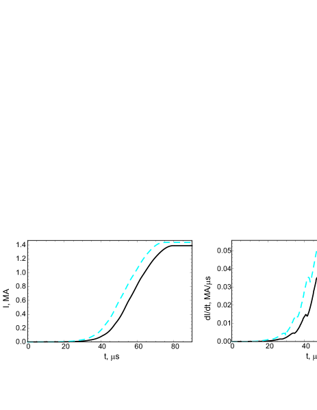
Figure 5: Current and current derivative calculated for HFCG with winding of type 2 at 1000 A initial current: ”pressure” option (solid curve) and ”gurney” option (dashed curve)

V-B Comparison of simulation and experiment results

Two experimentally tested HFCGs enable evaluating simulation reliability.

HFCG#1:

• Winding: 3 sections of 85, 130 and 110 mm length; winded by wire of 1.06 mm diameter with one start, 1.4 mm diameter with one start and 1.4 mm diameter with three starts, respectively, and the coaxial end section of 100 mm length;

• Load inductance: 30 nHn;

• detonation velocity: 7.07 mm/$\mu$s;

• explosive density: 1470 kg/m³;

• Wire isolation thickness: 0.24 mm.

HFCG#2:

• Winding: 5 sections of 75, 65, 80, 65, 70 mm length; winded by wire of 1.06 mm diameter with one start,1.4 mm diameter with one start, 1.6 mm diameter with two and four starts and 1.4 mm diameter with eight starts, respectively, and the coaxial end section of 70 mm length;

• Load inductance: 147 nHn;

• detonation velocity: 7.9 mm/$\mu$s;

• explosive density: 1510 kg/m³;

• Wire isolation thickness: 0.24 mm.

Comparison of experimentally obtained current derivative curves and those calculated by FCGcalc with ”2D” and ”nonlinear” options is presented in Fig.6 and Fig.7. Each figure displays two plots: left one is for ”pressure” option and right is calculated for ”gurney” option. Experimental and simulated curves are aligned by the mark of last winding section joint with the coaxial end section. Calculated with ”pressure” option current derivative gives better fit for experimental curve for both experiments. Dashed lines in both figures mark the instant when HFCG conductors temperature reached copper melting point (overheating mark). Significant difference in simulated and experimentally obtained curves arises in the vicinity of overheating mark and apparently is explained by insufficiency for the extreme conditions. The latter also explains the negative spike on simulated curve for HFCG#1.

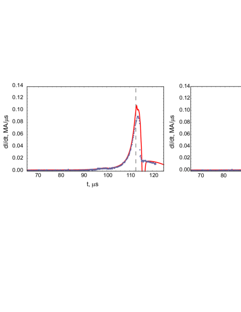
Figure 6: Current derivative for HFCG#1 at 700 A initial current and purely inductive load 32nH: calculated (solid curve) and experimentally measured (dotted curve). Left plot is for ”pressure” option and right one is for ”gurney” option

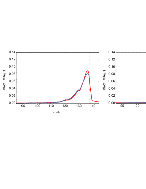
Figure 7: Current derivative for HFCG#2 at 800 A initial current and purely inductive load 147nH: calculated (solid curve) and experimentally measured (dotted curve). Left plot is for ”pressure” option and right one is for ”gurney” option.

VI Conclusion

Diverse approaches to HFCG’s inductance,resistance and armature expansion calculating are evaluated and some evaluating conclusions can be made.

Inductance calculation by 1D model can be used when HFCG inductance at a contact point approaching the coaxial end section is comparable with the load inductance. The time difference provided by different models for armature expansion description should be kept in mind, when aligning experimental curves with simulated those. Consideration of armature acceleration under the pressure of detonation products increases accuracy of HFCG simulation. Control of HFCG temperature during simulation enables detecting critical points of system operation.

References

- [1] C. M. Fowler and R. S. Caird, The Mark IX Generator, In: R. White, B. H. Bernstein (eds.), Digest of Technical Papers of the 7th IEEE Pulsed Power Conf., New York, IEEE Press (1989), pp. 475-478.
- [2] B M Novac, I R Smith, M Enache and H R Stewardson, “Simple 2D model for helical flux compression generators”, Laser Particle Beams, vol. 15, pp. 379-395, 1997.
- [3] A.S. Pikar, Yu. N. Deryugin, P. V. Korolev, V. M. Klimashov, The Method for Numerical Modeling of Magnetic Field Compression in HFCG, (in Russian) Proc. of the VI Zababahin’s Scientific Readings, Sarov, VNIIEF, 2001.
- [4] D.E. Lileikis, Numerical simulation of a helical, explosive flux compression generator, Plasma Science, 1997. IEEE Conference Record – Abstracts. p. 276.
- [5] G.F. Kiuttu, J.B. Chase, An armature-stator contact resistance model for explosively driven helical magnetic flux compression generators // IEEE Pulsed Power Conference 2005. P. 435-440
- [6] A. A. Neuber (ed), Explosively Driven Pulsed Power: Helical Flux Compression Generators, Berlin Heidelberg , Springer-Verlag (2005).
- [7] H. E. Knoepfel, Magnetic Fields: A Comprehensive Theoretical Treatise for Practical Use, New York, John Wiley & Sons, Inc (2000).
- [8] R. W. Gurney. The Initial Velocities of Fragments from Bombs, Shell, and Grenades. Aberdeen Proving Ground, Md.: Ballistic Research Laboratories, 1943.
- [9] L. Orlenko, Fizika Vzryva V.1,2, Fizmatlit, 2004 [in Russian], ISBN-10: 5922102192, 5922102192; ISBN-13: 978-5922102193, 978-5922102193
- [10] A. I. Pavlovsky, R. Z. Lyudaev, A. S. Ryzhov, S. S. Pavlov, G. M. Spirov, N. P. Biyushkin, Multisectional generator MC-2, Megagauss III, Moscow, Nauka (1984) pp. 312-320.
- [11] V. E. Fortov (ed), Explosive-Driven Generators of Powerful Electrical Pulses, Cambridge, CISP (2007).
- [12] J. C. Maxwell. A Treatise on Electricity and Magnetism, 3rd ed., vol. 2. New York: Dover Publications, 1954, pp. 338-340.