Spectral-graph Based Classifications: Linear Regression for Classification and Normalized Radial Basis Function Network

Abstract

Spectral graph theory has been widely applied in unsupervised and semi-supervised learning. It is still unknown how it can be exploited in supervised learning. In this paper, we find for the first time, to our knowledge, that it also plays a concrete role in supervised classification. It turns out that two classifiers are inherently related to the theory: linear regression for classification (LRC) and normalized radial basis function network (nRBFN), corresponding to linear and nonlinear kernel respectively. The spectral graph theory provides us with a new insight into a fundamental aspect of classification: the tradeoff between fitting error and overfitting risk. With the theory, ideal working conditions for LRC and nRBFN are presented, which ensure not only zero fitting error but also low overfitting risk. For quantitative analysis, two concepts, the fitting error and the spectral risk (indicating overfitting), have been defined. Their bounds for nRBFN and LRC are derived. A special result shows that the spectral risk of nRBFN is lower bounded by the number of classes and upper bounded by the size of radial basis. When the conditions are not met exactly, the classifiers will pursue the minimum fitting error, running into the risk of overfitting. It turns out that $\ell_{2}$-norm regularization can be applied to control overfitting. Its effect is explored under the spectral context. It is found that the two terms in the $\ell_{2}$-regularized objective are one-one correspondent to the fitting error and the spectral risk, revealing a tradeoff between the two quantities. Concerning practical performance, we devise a basis selection strategy to address the main problem hindering the applications of (n)RBFN. With the strategy, nRBFN is easy to implement yet flexible. Experiments on 14 benchmark data sets show the performance of nRBFN is comparable to that of SVM, whereas the parameter tuning of nRBFN is much easier, leading to reduction of model selection time.

Keywords: classification, spectral graph, radial basis function network, linear regression, regularization, overfitting.

1 Introduction

Spectral graph theory is a theory that centers around the graph Laplacian matrix [14]. On the one hand, it can reveal underlying cluster structure of data by the eigenvectors of the Laplacian matrix, on the other hand, the eigenvectors can serve as dimensionally reduced codes that preserve pair-wise data relation. The theory has found wide applications in unsupervised learning, including clustering [65] (generally named spectral clustering, including, e.g., ratio cut (Rcut) [10] and normalized cut (Ncut) [58, 43]), and dimensionality reduction (e.g., Laplacian eigenmap (LE) [2] and locality preserving projections (LPP) [24]). Later, it develops as a popular paradigm in semi-supervised learning, including semi-supervised clustering [29, 34] and semi-supervised classification [72, 70, 3, 71]. In semi-supervised learning, in an attempt to impose pair-wise data relation, the role of spectral graph usually appears as a “graph-regularization” term added to the other objectives.

Recently it has been discovered that, in the scope of unsupervised learning, spectral graph theory unifies a series of elementary methods of machine learning into a complete framework [25]. The methods cover dimensionality reduction, cluster analysis, and sparse representation. They range from principal component analysis (PCA) [28], K-means [38], LE [2], Rcut [10], and a new spectral sparse representation (SSR) [25]. It is revealed that these methods share inherent relations, they even become equivalent under an ideal graph condition. The framework also incorporates extended relations to conventional over-complete sparse representations [19], e.g., [45], method of optimal directions (MOD) [21], KSVD [1]; manifold learning, e.g., kernel PCA [56], multidimensional scaling (MDS) [16], Isomap [62], locally linear embedding (LLE) [54]; and subspace clustering, e.g., sparse subspace clustering (SSC) [20], low-rank representation (LRR) [36].

However, as far as we know, spectral graph theory has not yet found applications in supervised classification, except in hybrid-model way where the relation is not inherent, e.g., the addition of certain classification objective with a graph-regularization term. It is interesting to know whether the theory plays a concrete role in supervised classification and which classifiers are related.

In supervised learning, linear regression and radial basis function network (RBFN) are two basic methods. Both of them are devoted to function fitting, including classification as special case. It is well-known that linear regression can be interpreted with Bayesian probability (see, e.g., [6]), and when used for classification (LRC), its link to linear discriminant analysis was already discovered [68]. RBFN [51, 8, 39] and its normalized variant (nRBFN) [39, 60] are classical neural networks well-known for their simple structures and universal function approximation capacities [48, 67, 4]. Among broad connections to many theories [7], RBFN can be interpreted with Tikhonov regularization theory [50], while nRBFN can be interpreted with kernel regression [60, 67]. However, the above methods are hardly related to spectral graph theory before.

In classification application, it has been repeatedly demonstrated that [53, 47, 22, 52] the performance of RBFN can be comparable to support vector machine (SVM) [15]. Especially, in a comprehensive evaluation involving 179 classifiers and 121 data sets by [22], RBFN ranks third, immediately following SVM. However, despite of bearing additional advantages, (n)RBFN did not receive wide applications as SVM. This situation may be attributed to: (1) the less sound theoretical background compared with SVM, (2) the basis selection problem involved in (n)RBFN design [13, 46, 55, 47, 52], and (3) the difficulty of parameter tuning. In this paper, in addition to exploring stronger theoretical background for (n)RBFN, to make (n)RBFN become practical tool, we propose a solution scheme for the basis selection and parameter setting problems.

1.1 Our Work

In this paper, we uncover the concrete role of spectral graph theory in supervised classification, and find that LRC and nRBFN are inherently related to the theory. The tradeoff between fitting error and overfitting risk is a fundamental problem of classification. The theory provides us with a new insight into this problem under the context of LRC and nRBFN. With the theory, we establish the ideal working conditions for the two classifiers, which ensure not only zero fitting error but also low overfitting risk. When the conditions are not met exactly, the $\ell_{2}$-norm regularization can be applied to control overfitting, its effect is revealed under the spectral context. As a benefit, the regularization weight can be set in a principled and easy way. The followings are more detailed introduction.

In spectral clustering, we directly extract the cluster information from the eigenvectors of Laplacian matrix, i.e., recover the indicator vectors from the eigenvectors. However, in classification, the partition of data is assigned, and the indicator vectors are given, it seems not straightforward to see how spectral graph theory will work in this case. It turns out that we are to find the closest components in the eigenspace of Laplacian matrix to approximate the given indicator vectors. If the data is well-behaved, i.e., the given classes match the underlying clusters, then unsupervised clustering and supervised classification become consistent, and they unify under the spectral graph framework.

In this paper, we find that LRC and nRBFN are inherently related to spectral graph theory. Firstly, LRC will lay down some theoretical foundation, then nRBFN is derived via applying kernel trick on LRC. Broadly speaking, the data/feature matrix used by LRC/nRBFN shares the same eigenvectors with the Laplacian matrix, and we are to find the closest components in the eigenvectors to approximate the given indicator vectors. When an ideal graph condition is satisfied, which requires the classes being totally separated, the indicator vectors appear in the leading eigenspace of largest eigenvalues, and consequently zero fitting error is achieved. That is the inherent relation of LRC and nRBFN to spectral graph theory.

Although, zero fitting error is desirable, classification is more concerned with generalization performance. Striking a balance between low fitting error and low overfitting risk is a critical problem. Under the ideal graph condition, things are perfect, the fitting error is zero and the overfitting risk is low. From qualitative point of view, this is because the indicator vectors are found in the principal subspace. The principal subspace corresponds to stable features, as contrary to the minor subspace that corresponds to noisy features, especially when sampling is insufficient. For quantitative analysis, we define two concepts: the fitting error and the spectral risk. The spectral risk measures the deviation of the found components to the principal subspace, therefore it signals a warning of overfitting. The bounds of the two quantities for nRBFN and LRC are derived. A special result shows that the spectral risk of nRBFN is lower bounded by the number of classes–a quantity representing “problem complexity”, and upper bounded by the size of basis–a quantity representing “model complexity”. The upper bound indicates a tradeoff between fitting error and overfitting risk: larger basis implies lower error but higher risk.

In practice, the ideal condition cannot be met exactly, the leading eigenspace will deviate from the target indicator vectors. The found closest components may lie in minor subspace of small singular values. It is easily prone to noise, giving rise to increment of overfitting risk. It will be shown that the $\ell_{2}$-norm regularization can alleviate this problem. Its effect is explored under the spectral context. First, qualitatively, it drives the classifier to find the closest components in the principal subspace and discourages the opposite direction. Second, quantitatively, the two terms in the $\ell_{2}$-regularized objective are in one-one correspondence to the fitting error and the spectral risk, showing a tradeoff between the two quantities.

nRBFN is more powerful than LRC for its nonlinear kernel and significant risk bounds, we thus focus on nRBFN. To make nRBFN work in practice, we devise a basis selection strategy to address the main problem that hinders the wide applications of (n)RBFN. The strategy is based on soft K-nearest neighbors. It is easy to implement and the result is deterministic, in contrast to traditional K-means based strategy that depends on random initialization. Traditionally, setting the basis size is a troublesome problem. In our scheme, it is implicitly determined via a user-friendly threshold within range $(0,1]$. With this threshold, the basis size can be automatically determined according to the complexity of data distribution. We can also flexibly control the tradeoff between accuracy and computational cost via this threshold. Besides, when using $\ell_{2}$-norm regularization, the regularization weight can be set in a more principled way. In all, the parameter tuning is easy, leading to significant reduction of model selection time.

The contributions of the paper are as follows:

1. We have extended the spectral graph framework to the supervised classification domain. We found for the first time, to our knowledge, that spectral graph theory plays a concrete role in supervised classification. Two classifiers, LRC and nRBFN, corresponding to linear and nonlinear kernel respectively, turn out to be inherently related to the theory. With the theory, ideal working conditions for LRC and nRBFN are presented, which ensure not only zero fitting error but also low overfitting risk.

2. With the spectral graph theory, new insights into the overfitting problem as well as the effect of $\ell_{2}$-norm regularization are obtained. For quantitative analysis, two concepts, the fitting error and the spectral risk have been defined. The bounds of them for nRBFN and LRC have been derived. One result states that the spectral risk of nRBFN is lower bounded by the number of classes and upper bounded by the size of radial basis. In addition, it turns out that the two terms in the $\ell_{2}$-regularized objective are one-one correspondent to the fitting error and the spectral risk, revealing a tradeoff between the two quantities.

3. We have devised a basis selection strategy for (n)RBFN, so that nRBFN becomes easy to implement yet flexible. The performance of nRBFN is comparable to that of SVM, whereas the parameters of nRBFN are much easier to set, leading to significant reduction of model selection time.

The rest of the paper is organized as follows. Section 2 briefly introduces spectral graph theory and reviews its rationale for clustering. Section 3 presents spectral-graph based classifications, including linear version LRC and kernel version nRBFN. Meanwhile, the ideal working conditions are introduced. In the cases of the conditions are not met exactly, Section 4 introduces the $\ell_{2}$-norm regularization for LRC and nRBFN. Section 5 defines the fitting error and spectral risk, derives their bounds for nRBFN and LRC, and reveals the effect of $\ell_{2}$-norm regularization. Section 6 proposes the basis selection strategy. Section 7 demonstrates the performance of nRBFN and empirically evaluates the fitting error and spectral risk. Section 8 introduces some related work. The paper is ended with further work in Section 9.

Notations. $A=[A_{1},\dots,A_{n}]\in\mathbb{R}^{p\times n}$: data matrix with $n$ samples of dimension $p$. $F=[F_{1},\dots,F_{n}]\in\mathbb{R}^{K\times n}$: indicator matrix for $n$ samples of $K$ classes. If the $i$th sample belongs to class $k$, then the $k$th entry of $F_{i}$ is one and the others are zero. $G=[G_{1},\dots,G_{r}]\in\mathbb{R}^{p\times r}$: basis vectors of RBFN and nRBFN. $\mathbf{1}$: a vector of uniform value 1. $\operatorname{diag}(v)$: a diagonal matrix formed by vector $v$.

2 Spectral-graph Based Clustering: a Review

Given an undirected graph of $n$ vertices (data points), with the adjacency matrix defined to be a similarity matrix $W\in\mathbb{R}^{n\times n}$, measuring the pairwise similarities between data points, $W_{ij}=W_{ji}\geq 0$, the Laplacian matrix is defined as $L\doteq S-W$, where $S$ is a diagonal degree matrix with the diagonal being the sum of weights of each vertex, i.e., $S=\operatorname{diag}(\mathbf{1}^{T}W)$. The Laplacian matrix has the following properties [65].

1. It is positive semi-definite.

2. Vector $\mathbf{1}$ is always an eigenvector with eigenvalue zero.

3. Assume there are $K$ connected components in the graph, then the indicator vectors of these components (row vectors of $F$) span the eigenspace of eigenvalue zero.

These properties are exploited for clustering purpose [65]. Assume we are to find $K$ clusters, if the ideal graph condition for clustering (Definition 1) [25] holds (the condition implies the between-cluster weights are all zero: $W_{ij}=0$, if the $i$th and $j$th points are of different clusters), then we can compute the $K$ eigenvectors of $L$ with the smallest eigenvalues (zero), and then postprocess these eigenvectors to finish clustering. In practice, the $K$ components of the graph may not be completely disconnected. In this noisy case, the same procedure can still be applied, since the $K$ eigenvectors with the smallest eigenvalues become rotated noisy indicators, which may not differ much to their ideal ones. This is the working rationale of spectral clustering.

Definition 1.

(ideal graph condition for clustering) Targeting for $K$ clusters, if there are exactly $K$ connected components in the graph, then the graph (or similarity matrix) is called ideal (with respect to $K$ clusters).

Finally, the eigenvectors of $L$ with eigenvalue zero (smallest) are the eigenvectors of $S^{-1}W$, called normalized Laplacian matrix, with eigenvalue one (largest) [65].

3 Spectral-graph Based Classifications

In spectral clustering, we directly extract the cluster information from the eigenvectors of Laplacian matrix, i.e., recover the indicator vectors from the eigenvectors. However, in classification, the indicator vectors are given. It will be shown that we are to find the closest components in the eigenspace to approximate the indicator vectors. When an ideal condition is satisfied, the indicator vectors appear in the leading eigenspace, achieving zero fitting error and low overfitting risk.

3.1 Linear Version: Linear Regression for Classification (LRC)

We will show that the singular vectors of the data matrix are the eigenvectors of a Laplacian matrix. Thus the link to spectral graph theory is established. The Laplacian matrix is built by the inner product between data, i.e., linear kernel. In the following, we first introduce the basic formulation of LRC, then analyze it from the row-space view, this leads to the relation to spectral graph theory. Based on the theory, an ideal working condition for LRC is presented. Finally, we analyze LRC from the column-space view, which paves the way to nRBFN.

3.1.1 Basic Formulation

Given data matrix $A$ (assume mean-removed, $A\mathbf{1}=0$) and the corresponding class labels, we convert the labels to an indicator matrix $F$, and define an augmented data matrix $\tilde{A}=\begin{bmatrix}\sqrt{\beta}\mathbf{1}^{T}\\ A\end{bmatrix}$ [25], where $\beta$ is a constant scalar that will be introduced later. The objective of LRC is to find a weight matrix $D$ so that the linear combinations of the columns of $D$ and the samples approximate the indicator vectors:

$$\min_{D}\,\sum_{i=1}^{n}\|F_{i}-D\tilde{A}_{i}\|_{2}^{2}=\|F-D\tilde{A}\|_{F}^{2}.$$ (1)

Provided $\operatorname{rank}(\tilde{A})=p+1$, there is a unique closed-form solution: $D^{*}=F\tilde{A}^{T}(\tilde{A}\tilde{A}^{T})^{-1}$ [6]. After $D^{*}$ is obtained, given a test sample $b$ (with mean removed as $A$), its label is determined by the maximum entry of $D^{*}\tilde{b}$:

$$\mathop{\arg\max}_{k}\,(D^{*}\tilde{b})_{k}.$$ (2)

It can be shown that the sum of $D^{*}\tilde{b}$ is always one. Besides, $D^{*}\tilde{b}$ is an approximation to the indicator vector. These endow $D^{*}\tilde{b}$ with a quasi-probability interpretation (may include negative values).

3.1.2 Row-space View

It will be shown that LRC are to find the closest components in the data row-space to approximate the indicator vectors, and this relates to the spectral graph.

Substituting $D^{*}$ into (1), we obtain $\|F-F\tilde{A}^{T}(\tilde{A}\tilde{A}^{T})^{-1}\tilde{A}\|_{F}^{2}$. Note that $\tilde{A}^{T}(\tilde{A}\tilde{A}^{T})^{-1}\tilde{A}$ is a projection matrix, and the projection subspace is spanned by the rows of $\tilde{A}$. In this view, to approximate $F$, LRC projects $F$ onto the row-space of $\tilde{A}$ and reconstructs. These facts are well-known. However, a natural question arises: does the row-space contain “ingredients” close to $F$, so that the reconstruction error is small? With spectral graph theory, we present an ideal condition under which the row-space of $\tilde{A}$ contains $F$. Define a similarity matrix $W\doteq\tilde{A}^{T}\tilde{A}$, and

$$\beta\doteq-\min_{ij}\,(A^{T}A)_{ij}.$$ (3)

Since the data is mean-removed, we have $\min_{ij}\,(A^{T}A)_{ij}<0$, $\beta$ thus defined makes $W$ become nonnegative [25]. The condition and theorem are as follows:

Definition 2.

(ideal graph condition for classification) If the weights between vertices of different classes are all zero, i.e., $\forall i,j$, $W_{ij}=0$ if $F_{i}\neq F_{j}$, then the graph (or similarity matrix) is called ideal (with respect to the class labels).

Theorem 1.

Given indicator matrix $F$, if $W$ satisfies the ideal graph condition for classification, then the row vectors of $F$ lie in the row-space of $\tilde{A}$ corresponding to the largest singular value ($\sqrt{\beta n}$), and therefore zero fitting error is achieved: $F=D^{*}\tilde{A}$.

Proof.

$W$ such defined is a nonnegative symmetric matrix, hence it is a qualified similarity matrix. Because $A$ is mean-free, the degree matrix is $S=\operatorname{diag}(\mathbf{1}^{T}W)=n\beta I$, and the Laplacian matrix $L\doteq S-W$ becomes $n\beta I-\tilde{A}^{T}\tilde{A}$. Assume the thin SVD [23] of $A$ to be $U\Sigma V$, where the singular values are arranged in descending order, then [25]

$$\tilde{A}=\tilde{U}\tilde{\Sigma}\tilde{V}=\begin{bmatrix}1&\\ &U\end{bmatrix}\begin{bmatrix}\sqrt{\beta n}&\\ &\Sigma\end{bmatrix}\begin{bmatrix}\frac{1}{\sqrt{n}}\mathbf{1}^{T}\\ V\end{bmatrix},$$ (4)

Further, by $L=n\beta I-\tilde{A}^{T}\tilde{A}$, we obtain the spectral decomposition [23] of $L$:

$$\begin{split}L=\begin{bmatrix}\frac{1}{\sqrt{n}}\mathbf{1}&V^{T}&\hat{V}^{T}\end{bmatrix}\begin{bmatrix}0&&\\ &\beta nI-\Sigma^{2}&\\ &&\beta nI\end{bmatrix}\begin{bmatrix}\frac{1}{\sqrt{n}}\mathbf{1}^{T}\\ V\\ \hat{V}\end{bmatrix},\end{split}$$ (5)

where $\hat{V}$ is the complement of $\tilde{V}$.

If the condition holds, by the third property of Laplacian matrix in Section 2, the row vectors of $F$ lie in the eigenspace of $L$ with eigenvalue zero. In view of (5) and (4), the eigenvectors of $L$ with the smallest eigenvalues are the right singular vectors of $\tilde{A}$ with the largest singular values. Thus, the row vectors of $F$ lie in the row-space of $\tilde{A}$ with the largest singular values (all equal $\sqrt{\beta n}$). ∎

Note that the condition ensures not only perfect reconstruction but also that the target lies in the principal row-subspace of data, or principal components (PCs) in the language of PCA [28]. This is important, because the PCs correspond to stable features, whereas the minor components usually correspond to noise, especially when sampling is insufficient. In some cases, zero training error can be achieved, however, the target may be found in the minor subspace, then generalization error can be large. That is the overfitting problem. We will return to this issue in later sections.

3.1.3 Column-space View

Finally, we take a closer look at the vector $D^{*}\tilde{b}$, and understand the voting mechanism of LRC. The facts are routine. With (4), we have $D^{*}\tilde{b}=F\tilde{V}^{T}\tilde{V}_{b}=\sum_{i=1}^{n}F_{i}(\tilde{V}_{i}^{T}\tilde{V}_{b})$, where $\tilde{V}_{b}=\tilde{\Sigma}^{-1}\tilde{U}^{T}\tilde{b}$ are the normalized full PCs of $\tilde{b}$ and $\tilde{V}_{i}$ are those of $\tilde{A}_{i}$. The mechanism of class prediction becomes clear: the class of a sample is determined by the votes of the training set, where the indicator vectors $F_{i}$’s play the role of the votes, and the similarities between the training set and the sample serve as the weights assigned to the votes. Here, the similarity is measured by the inner product of PCs. For general data, this is not a good choice, and that is one of the limitations of LRC. We now introduce the more powerful kernel version, which measures the similarity based on Euclidean distance.

3.2 Kernel Version: Normalized RBF Network (nRBFN)

We will apply the kernel trick to LRC in two ways: a traditional way leads to RBFN, the other way leads to nRBFN. The function matrix used by RBFN is the similarity matrix, while that used by nRBFN is the normalized Laplacian matrix. Since the similarity matrix does not share the properties of Laplacian matrix, we cannot directly analyze RBFN by spectral graph theory, whereas the link of nRBFN to the theory is straightforward. In a following subsection, we introduce the routine basis reduction to reduce the size of the networks. After that, we interpret nRBFN from the row-space and column-space views, and analyze it with spectral graph theory. An ideal working condition in the context of basis reduction is introduced, and some properties of nRBFN are shown.

3.2.1 RBFN

We derive RBFN by applying kernel trick to LRC. The solution of (1) can be rewritten as $D^{*}=(F\tilde{A}^{T}(\tilde{A}\tilde{A}^{T})^{-2}\tilde{A})\tilde{A}^{T}$, which is a linear combination of the training data. If we assume $D=X\tilde{A}^{T}$, then (1) turns into another objective

$$\min_{X}\,\|F-X\tilde{A}^{T}\tilde{A}\|_{F}^{2}.$$ (6)

Applying kernel trick on $\tilde{A}^{T}\tilde{A}$, we get

$$\min_{X}\,\|F-XW\|_{F}^{2}.$$ (7)

$W$ is a kernel matrix defined by some kernel function $W_{ij}=\phi(A_{i},A_{j})$. In LRC case, it is a linear function $\phi(A_{i},A_{j})=A_{i}^{T}A_{j}+\beta$. Among nonlinear ones, Gaussian kernel is most frequently used $\phi(A_{i},A_{j})=\exp\{-\|A_{i}-A_{j}\|_{2}^{2}/(2\sigma^{2})\}$. (7) is an RBFN [51, 8, 39], where the kernel function is viewed as radial basis function $\varphi(\|G_{i}-x\|)$: each column of $W$ corresponds to a sample $x$, while each row a basis vector $G_{i}$. Here, the basis $G$ consists of the whole training set, $G_{i}=A_{i}$. Assume $W$ has full rank, the solution of (7) is $X^{*}=FW^{-1}$. Given a sample $b$, since $D^{*}\tilde{b}=X^{*}\tilde{A}^{T}\tilde{b}$, applying the same trick, the class of $b$ is decided by

$$\mathop{\arg\max}_{k}\,(X^{*}W_{b})_{k},$$ (8)

where $(W_{b})_{i}=\phi(A_{i},b)$.

For RBFN, the ideal graph condition does not work, since the kernel matrix when served as similarity matrix does not possess the same properties as its Laplacian matrix. We are not sure whether $F$ lies in the principal subspace or minor subspace.

3.2.2 nRBFN

We restart the derivation with kernel trick from another way, which will lead to nRBFN. By absorbing $\beta n$ into $X$, (6) is equivalent to

$$\min_{X}\,\|F-X\tilde{A}^{T}\tilde{A}(\beta n)^{-1}\|_{F}^{2}=\min_{X}\,\|F-X\tilde{A}^{T}\tilde{A}\,\operatorname{diag}(\mathbf{1}^{T}\tilde{A}^{T}\tilde{A})^{-1}\|_{F}^{2}.$$ (9)

Note that $\tilde{A}^{T}\tilde{A}\,\operatorname{diag}(\mathbf{1}^{T}\tilde{A}^{T}\tilde{A})^{-1}=WS^{-1}$, which is the transpose of the normalized Laplacian matrix. Applying kernel trick and using Gaussian kernel, we obtain nRBFN:

$$\min_{X}\,\|F-XWS^{-1}\|_{F}^{2}.$$ (10)

Assume $W$ has full rank, the solution is $X^{*}=FSW^{-1}$. Given a sample $b$, since $X^{*}\tilde{A}^{T}\tilde{b}(\beta n)^{-1}=X^{*}\tilde{A}^{T}\tilde{b}(\mathbf{1}^{T}\tilde{A}^{T}\tilde{b})^{-1}$, applying the same kernel trick, the class of $b$ is decided by

$$\mathop{\arg\max}_{k}\,(X^{*}W_{b}(\mathbf{1}^{T}W_{b})^{-1})_{k}=\mathop{\arg\max}_{k}\,(X^{*}W_{b}/s_{b})_{k},$$ (11)

where $s_{b}$ is the sum of $W_{b}$.

Note that $WS^{-1}$ is a normalized similarity matrix. Each column of it sums to one, so is $W_{b}/s_{b}$. nRBFN was initially mentioned by [39] and later derived from probability density estimation and kernel regression by [59, 60, 67]. It is also closely related to Gaussian mixture model [63]. However, the underlying spectral graph background seems not yet be discovered. Before the exploration, we deal with the basis reduction problem.

3.2.3 Basis Reduction

In above, the bases of RBFN and nRBFN consist of the whole training set, which will lead to expensive computation. Traditionally, basis reduction is applied [52]. A smaller basis is chosen by some strategy (discussed in Section 6). For the moment, we assume the basis $G=[G_{1},\dots,G_{r}]$, $r<n$, is given. Now, $W$ is of size $r\times n$, and $W_{ij}=\phi(G_{i},A_{j})$. Denoting

$$\tilde{W}\doteq WS^{-1}\in\mathbb{R}^{r\times n},$$

the formulation of basis-reduced nRBFN becomes

$$\min_{X}\,\|F-X\tilde{W}\|_{F}^{2}.$$ (12)

nRBFN and RBFN are special cases of linear regression, with sample vectors replaced by similarity vectors. Assume $W$ is of full rank, the solution of nRBFN is $X^{*}=F\tilde{W}^{T}(\tilde{W}\tilde{W}^{T})^{-1}$ (that of RBFN is $X^{*}=FW^{T}(WW^{T})^{-1}$). Given a sample $b$, in nRBFN its class is decided by

$$\mathop{\arg\max}_{k}\,(X^{*}\tilde{W}_{b})_{k},$$ (13)

where $\tilde{W}_{b}\doteq W_{b}/s_{b}$, $W_{b}$ are the similarities between $b$ and the basis, and $s_{b}$ is the sum of $W_{b}$.

Hereafter, we focus on basis-reduced nRBFN.

3.2.4 Row-space View and Column-space View to nRBFN

We will show the spectral graph theory underlying nRBFN, and introduce some basic properties as well as interpretations concerning nRBFN.

1. From column-space view, we will show that, as LRC, the class prediction of nRBFN is also via voting mechanism. First, besides $\tilde{W}$ has a probability interpretation, the weight matrix $X^{*}$ also has a quasi-probability interpretation. We have

Lemma 2.

Each column of the weight matrix $X^{*}$ sums to one: $\mathbf{1}^{T}X^{*}=\mathbf{1}^{T}F\tilde{W}^{T}(\tilde{W}\tilde{W}^{T})^{-1}=\mathbf{1}^{T}$.

Proof.

The row-space of $\tilde{W}$ contains $\mathbf{1}^{T}\in\mathbb{R}^{1\times n}$, because $\mathbf{1}^{T}\tilde{W}=\mathbf{1}^{T}$. Thus, from the projection point of view, $\mathbf{1}^{T}\tilde{W}^{T}(\tilde{W}\tilde{W}^{T})^{-1}\tilde{W}=\mathbf{1}^{T}$. By this, $\mathbf{1}^{T}X^{*}\tilde{W}=\mathbf{1}^{T}$. On the other hand, since $\tilde{W}$ has full rank, the solution of $x\tilde{W}=\mathbf{1}^{T}$ is unique. However, both $\mathbf{1}^{T}\in\mathbb{R}^{1\times r}$ and $\mathbf{1}^{T}X^{*}$ are the solutions, so we conclude $\mathbf{1}^{T}X^{*}=\mathbf{1}^{T}$. ∎

Now considering (13), the class of sample $b$ is decided by the voting of the basis. Each basis vector keeps a vote $X^{*}_{i}$, and the weight assigned to the vote is the normalized similarity of $b$ to that basis vector $G_{i}$. In contrast to LRC, the votes are not indicator vectors, and the weights are not computed by inner product. Rather, the votes of the basis are gathered from another voting of the training data, $X^{*}_{i}=F(\tilde{W}^{T}(\tilde{W}\tilde{W}^{T})^{-1})_{i}$. Note that $\mathbf{1}^{T}\tilde{W}^{T}(\tilde{W}\tilde{W}^{T})^{-1}=\mathbf{1}^{T}$, since $\mathbf{1}^{T}X^{*}=\mathbf{1}^{T}$. We can expect that when a basis vector is more “reliable”, e.g., lying in the center of a class, the vote it keeps would concentrate in its class, whereas when lying in the overlapping region, the vote would be distributed more evenly. Generally, except under the ideal condition below, $X^{*}$ will include negative value, which represents objection.

2. From row-space view, similar to LRC, nRBFN finds the closest subspace in the row-space of $\tilde{W}$ to approximate $F$. Again, an ideal condition ensuring perfect reconstruction exists. However, in the context of basis reduction, the graph should be generalized to a bipartite graph: one side of the vertices consists of the basis, the other side consists of the training set. We should assume the basis is a subset of the training set, and each class is represented by at least one basis vector. The original case where the basis consists of the whole training set is a special case of bipartite graph. Denoting $F_{G_{i}}$ to be the indicator vector of $G_{i}$, the condition is as follows:

Definition 3.

(ideal bipartite-graph condition for classification) If the weights between basis vertices and data vertices of different classes are all zero, i.e., $\forall i,j$, $W_{ij}=0$ if $F_{G_{i}}\neq F_{j}$, then the bipartite-graph (or similarity matrix) is called ideal (with respect to the class labels).

With these prerequisites, we have the following theorem indicating zero fitting error:

Theorem 3.

Given indicator matrix $F$, if $W$ satisfies the ideal bipartite-graph condition for classification, then the row vectors of $F$ lie in the row-space of $\tilde{W}$, and zero fitting error is achieved: $F=X^{*}\tilde{W}$.

The proof of the theorem is manifest: the rows of $\tilde{W}$ corresponding to the same class sum to an indicator vector of that class.

When the condition holds, it can be proved that the votes $X^{*}$ become an indicator matrix. In this case the votes are ideal and very confident, since they concentrate in one class.

Proposition 4.

If the ideal bipartite-graph condition for classification holds, $X^{*}$ becomes an indicator matrix. For basis vector $G_{i}$, $X^{*}_{i}=F_{G_{i}}$.

Proof.

Without loss of generality, assume the training samples of the same class are arranged consecutively, then $\tilde{W}$ is block-diagonal, so is $(\tilde{W}\tilde{W}^{T})^{-1}$. Further, $\tilde{W}^{T}(\tilde{W}\tilde{W}^{T})^{-1}$ has the same nonzero blocks as $\tilde{W}^{T}$. Since $X^{*}_{i}=F(\tilde{W}^{T}(\tilde{W}\tilde{W}^{T})^{-1})_{i}$, we see that $X^{*}_{i}$ is a linear combination of the indicator vectors of the same class as $G_{i}$, which means there is only one nonzero in $X^{*}_{i}$. By Lemma 2, we conclude that the nonzero value is one. Therefore, $X^{*}_{i}$ is an indicator vector of $G_{i}$. ∎

When the condition does not hold exactly, that is when the classes have some overlapping but not heavy, negative values may present in $X^{*}$, but their magnitude should be small, because $X^{*}$ is a continuous function of $W$.

Unlike LRC case, whether $F$ lies in the leading row-subspace is less obvious. When the basis consists of the whole training set and the ideal condition is satisfied, by property of the normalized Laplacian matrix (Section 2), rows of $F$ are the left eigenvectors with the largest eigenvalues. We expect they are close to the leading row-subspace that corresponds to the largest singular values. For the general bipartite-graph case, please refer to Appendix A for detailed investigation. We present the main result below.

Theorem 5.

Under the ideal bipartite-graph condition for classification, the row vectors of $F$ become the right singular vectors of $\tilde{W}$ corresponding to the largest singular values, if and only if the row sums of $\tilde{W}$ are even within each class: $\sum_{k}\tilde{W}_{ik}=\sum_{k}\tilde{W}_{jk}$, $\forall i,j,F_{G_{i}}=F_{G_{j}}$.

The theorem suggests that when designing the model, a balanced system, which means the row sums of $\tilde{W}$ are as even as possible within each class, is preferred.

Hereafter, without confusion, we will simply refer the above three conditions as ideal graph condition.

4 Regularization for LRC and nRBFN

In practice, the ideal graph conditions are not easy to meet exactly. In this case, zero fitting error may not be achieved, and part of the found closest components may lie in the minor subspace. This will lead to the increment of overfitting risk. In this section, we introduce the traditional $\ell_{2}$-norm regularization, and qualitatively show its effect on controlling the overfitting risk from the spectral view. The regularized versions of LRC and nRBFN are what we will really apply in real world.

4.1 Regularized LRC

For LRC, the ideal graph condition is hard to meet, except perhaps for high-dimensional data: by the construction of $W$, the condition essentially requires that, after translating along a new dimension, different classes become orthogonal. Thus in general case, the leading row-subspace of $\tilde{A}$ may deviate much from $F$. LRC then searches the entire row-space to find a closest subspace to approximate $F$. The found subspace may correspond to small singular values, which may represent discriminative features or, more frequently, noise (e.g., due to insufficient sampling). In other words, LRC may deem the noisy components of data as the discriminative features for classification. Poor generalization ability can be expected.

In this regard, we would like to encourage LRC to search within the principal row-subspace. This can be achieved via $\ell_{2}$-norm regularization:

$$\min_{D}\,\|F-D\tilde{A}\|_{F}^{2}+\lambda^{\prime}\|D\|_{F}^{2},$$ (14)

where $\lambda^{\prime}>0$ is a scalar weight. The unique closed-from solution is $D^{*}=F\tilde{A}^{T}(\tilde{A}\tilde{A}^{T}+\lambda^{\prime}I)^{-1}$, regardless of the rank of $A$. The label of a new sample is decided as (2).

In this case, the reconstruction of the training set is $D^{*}\tilde{A}=F\tilde{A}^{T}(\tilde{A}\tilde{A}^{T}+\lambda^{\prime}I)^{-1}\tilde{A}$. Assume the SVD of $\tilde{A}$ to be $\tilde{U}\tilde{\Sigma}\tilde{V}$, then $\tilde{A}^{T}(\tilde{A}\tilde{A}^{T}+\lambda^{\prime}I)^{-1}\tilde{A}=\tilde{V}^{T}\Lambda\tilde{V}$, where $\Lambda$ is a diagonal matrix with $\Lambda_{ii}=\tilde{\sigma}_{i}^{2}/(\tilde{\sigma}_{i}^{2}+\lambda^{\prime})<1$. For those large singular values $\tilde{\sigma}_{i}\gg\lambda^{\prime}$, $\Lambda_{ii}\approx 1$ so the principal subspace is preserved, while for those small ones $\tilde{\sigma}_{i}\ll\lambda^{\prime}$, $\Lambda_{ii}\approx 0$ so the minor components are suppressed. In implementation, for the ease of setting $\lambda^{\prime}$, we rewrite it to be $\lambda^{\prime}=\lambda\|\tilde{A}\|_{F}^{2}$. Note that $\|\tilde{A}\|_{F}^{2}=\sum_{i}\tilde{\sigma}_{i}^{2}$, so the contrast between $\tilde{\sigma}_{i}^{2}$ and $\lambda^{\prime}$ is easier to control. Back to the objective, $\|F-D^{*}\tilde{A}\|_{F}^{2}=\|F-F\tilde{V}^{T}\Lambda\tilde{V}\|_{F}^{2}$. Now LRC projects $F$ onto the principal row-subspace and reconstructs. The reconstruction error may increase slightly, but overfitting is alleviated. A quantitative analysis will be conducted in Section 5.

4.2 Regularized nRBFN

The ideal graph condition for nRBFN does not require orthogonality between the classes. Nevertheless, when the condition is not exactly met, to prevent nRBFN seeking the closest components in the minor subspace, we introduce regularization (the analysis follows LRC, and we omit):

$$\min_{X}\,\|F-X\tilde{W}\|_{F}^{2}+\lambda^{\prime}\|X\|_{F}^{2},$$ (15)

where $\lambda^{\prime}=\lambda\|\tilde{W}\|_{F}^{2}$, and $\lambda>0$ is a scalar weight. The solution becomes $X^{*}=F\tilde{W}^{T}(\tilde{W}\tilde{W}^{T}+\lambda^{\prime}I)^{-1}$, regardless of the rank of $\tilde{W}$. The label of a sample $b$ is decided as (13).

5 Error and Risk Analysis

The tradeoff between fitting error and overfitting risk is an important problem of classification. In this section, from the spectral point of view, we quantitatively analyze this problem for LRC and nRBFN, and reveal the effect of $\ell_{2}$-regularization further. First, we define a quantitative criterion, the spectral risk, for the measurement of overfitting risk. The fitting error is also formally defined. Next, we analyze the un-regularized nRBFN and LRC in mainly ideal cases. The bounds of the two quantities will be derived. Finally, we investigate the $\ell_{2}$-regularization (independent of the ideal graph condition). We will show that the two terms in the $\ell_{2}$-regularized objective are one-one correspondent to the fitting error and spectral risk, and study the effect of $\ell_{2}$-regularization on trading off the error and risk.

5.1 Definitions of Spectral Risk and Fitting Error

The definitions apply to linear regression, including LRC and nRBFN as special cases. We will define an absolute measure and a relative measure for both spectral risk and fitting error, the reasons will be clear later. The relative measures will be used as default definitions.

Let the linear regression problem be formulated as

$$\min_{D}\,\|F-DA\|_{F}^{2},$$ (16)

where $F\in\mathbb{R}^{K\times n}$ is any target matrix not limited to indicators, $A\in\mathbb{R}^{r\times n}$ ($r\leq n$) is any data matrix of full rank. The solution is $D^{*}=FA^{T}(AA^{T})^{-1}$. To exclude meaningless case, we assume $D^{*}\neq\mathbf{0}$, which means $FA^{T}\neq\mathbf{0}$, i.e., the data is not orthogonal to the target.

5.1.1 Spectral Risk

The spectral risk measures the deviation of the found components to the principal subspace. First, we define an absolute measure.

Definition 4.

(absolute spectral risk) The absolute spectral risk is defined as

$$\alpha\doteq\|D^{*}\|_{F}^{2}.$$ (17)

The justification can be understood by the following spectral expression. Assume the SVD of A to be $A=U\Sigma V$, then for problem (16), $D^{*}=FV^{T}\Sigma^{-1}U^{T}$, and we have

Proposition 6.

For linear regression problem (16),

$$\alpha=\sum_{i=1}^{r}\frac{a_{i}^{2}}{\sigma_{i}^{2}},$$ (18)

where $a_{i}^{2}$ is the projection of the target onto $V_{i}$: $a_{i}^{2}\doteq\sum_{k=1}^{K}(F_{k}V_{i}^{T})^{2}$, and $F_{k}$ is the $k$th row of $F$.

It implies that if the projections concentrate in the leading singular vectors, that is the closest components lie in the principal subspace, $\alpha$ will be small. Conversely, if they concentrate in the rear singular vectors, $\alpha$ will be large. Thus, as an absolute measure, $\|D^{*}\|_{F}^{2}$ is reasonable.

However, a meaningful range of the absolute measure cannot be determined. In order to cancel out the volume of data so that the measures between different data of the same model can be compared, we now define a relative measure by normalizing the projections and singular values.

Definition 5.

(spectral risk) The relative spectral risk, simply called spectral risk, is defined as

$$\gamma\doteq\frac{\|D^{*}\|_{F}^{2}\|A\|_{F}^{2}}{\|D^{*}A\|_{F}^{2}}.$$ (19)

For problem (16), by noting $\|A\|_{F}^{2}=\sum_{i=1}^{r}\sigma_{i}^{2}$ and $\|D^{*}A\|_{F}^{2}=\|FV^{T}V\|_{F}^{2}=\sum_{i=1}^{r}a_{i}^{2}$, we have

Proposition 7.

For linear regression problem (16),

$$\gamma=\sum_{i=1}^{r}\frac{\tilde{a}_{i}^{2}}{\tilde{\sigma}_{i}^{2}},$$ (20)

where $\tilde{a}_{i}^{2}\doteq a_{i}^{2}/\sum_{i=1}^{r}a_{i}^{2}$ and $\tilde{\sigma}_{i}^{2}\doteq\sigma_{i}^{2}/\sum_{i=1}^{r}\sigma_{i}^{2}$.

We can easily obtain the following range and bounds of $\gamma$:

Proposition 8.

The range of the spectral risk is $\gamma\geq 1$, and

$$1\leq\frac{1}{\tilde{\sigma}_{1}^{2}}\leq\gamma\leq\frac{1}{\tilde{\sigma}_{r}^{2}}.$$ (21)

The minimum value 1 is achieved, if and only if the data dimension is one, i.e., $r=1$.

The minimum bound implies that when we use the smallest basis having only one vector, the smallest risk is achieved. However, in this case, the fitting error can be quite large. There is a tradeoff between the fitting error and the spectral risk.

5.1.2 Fitting Error

First of all, it should be made clear that the fitting error is distinct from the error rate of classification. The absolute measure of fitting error is defined straightforwardly:

Definition 6.

(absolute fitting error) The absolute fitting error is defined as

$$f\doteq\|F-D^{*}A\|_{F}^{2}.$$ (22)

For problem (16), we have $f=\|F\|_{F}^{2}-\|D^{*}A\|_{F}^{2}=n-\sum_{i=1}^{r}a_{i}^{2}$. For reason that will be clear later, we define the relative measure to be:

Definition 7.

(fitting error) The relative fitting error, simply called fitting error, is defined as

$$\epsilon\doteq\frac{\|F-D^{*}A\|_{F}^{2}}{\|D^{*}A\|_{F}^{2}}+1.$$ (23)

For problem (16), the definition is equivalent to $\epsilon\doteq\|F\|_{F}^{2}/\|D^{*}A\|_{F}^{2}$. It is easy to see that

Proposition 9.

For linear regression problem (16), $\epsilon=n/\sum_{i=1}^{r}a_{i}^{2}$. Its range is $\epsilon\geq 1$. The minimum value 1 is achieved if and only if the row-space of data completely covers the target, i.e., $D^{*}A=A$.

5.2 Error and Risk Bounds of nRBFN

The ideal graph condition ensures zero fitting error and low overfitting risk, we will calculate the specific bounds for nRBFN (un-regularized), and then extend to the perturbation case where the condition is not satisfied exactly. We assume $F\tilde{W}^{T}\neq\mathbf{0}$, so that $X^{*}\neq\mathbf{0}$.

5.2.1 Ideal Case

Let $r_{k}$ denote the size of basis for the $k$th class, and $n_{k}$ the number of training samples of that class. We have the following result:

Theorem 10.

For nRBFN problem (12), when the ideal graph condition is satisfied, the fitting error achieves the minimum value, $\epsilon=1$, and the spectral risk has the bounds

$$\frac{r}{n}\sum_{k=1}^{K}\frac{n_{k}}{r_{k}}\leq\gamma\leq r.$$ (24)

The maximum risk is achieved when there is only one nonzero entry in each column of $\tilde{W}$. The minimum risk is approached when the entries in each column approach distributing uniformly within the corresponding class, it is achieved if and only if $r_{k}=1$ for all $k$.

Proof.

By Theorem 3, when the condition holds, perfect reconstruction is achieved, i.e., $X^{*}\tilde{W}=F$, so $\|X^{*}\tilde{W}\|_{F}^{2}=n$, $f=1$. Besides, by Proposition 4, $X^{*}$ becomes an indicator matrix, so $\|X^{*}\|_{F}^{2}=r$. The spectral risk then equals $r\|\tilde{W}\|_{F}^{2}/n$, depending only on $\|\tilde{W}\|_{F}^{2}$. Recall that each column of $\tilde{W}$ sums to one. For a vector $x\in\mathbb{R}^{p}$ with $\|x\|_{1}=1$, $1/\sqrt{p}\leq\|x\|_{2}\leq 1$, the upper bound is obtained when there is only one nonzero entry in $x$, while the lower bound is obtained when the entries distribute uniformly, i.e., $x_{i}=1/p$. Therefore, we get $\sum_{k=1}^{K}n_{k}/r_{k}\leq\|\tilde{W}\|_{F}^{2}\leq n$. The lower bound cannot be reached except when $r_{k}=1$ for all $k$, otherwise, the rank of $\tilde{W}$ will not be full, violating the assumption. ∎

Corollary 11.

If both $n_{k}$ and $r_{k}$ are uniform among the classes, i.e., $n_{k}=n/K$, $r_{k}=r/K$, for all $k$, (24) becomes

$$K\leq\gamma\leq r.$$ (25)

The corollary conveys clear implications. It tells that in the ideal case the spectral risk is lower bounded by the number of classes–a quantity representing “problem complexity”, and upper bounded by the size of basis–a quantity representing “model complexity”. First, the lower bound implies that however the model is the spectral risk will never be lower than the problem complexity. As the number of classes increases, the spectral risk increases too. By Theorem 10, the risk approaches the minimum when the system is balanced, i.e., when the entries are uniform. This is a stronger condition than the uniform row-sum condition in Theorem 5. Although they analyze the deviation of $F$ to the principal subspace by different manners, Theorem 10 by divisive manner while Theorem 5 by subtractive manner, the results are consistent. They both prefer a balanced system. Second, the upper bound implies a tradeoff between the fitting error and the overfitting risk: larger basis means lower error but higher risk. In addition, the size of basis also makes us recall the VC-dimension [64]–a classical measure of model complexity. Although the definitions are different, it happens that the VC-dimension of nRBFN (assuming the basis size is fixed, not a parameter) is also $r$. This shows some coincidence between the two concepts. Detailed comparisons are beyond the scope of the paper and we omit.

Although the conclusions hold for the ideal case, the theorem provides a foundation for the analysis of noisy case. We now explore.

5.2.2 Perturbation Case

We can deem the noisy case as perturbed from an ideal case, and then analyze it with matrix perturbation theory. As will be shown the noise is required to be only tiny.

Denote the noisy normalized similarity matrix to be $\tilde{W^{\prime}}$, it can be decomposed as $\tilde{W^{\prime}}=\tilde{W}+\Delta W$, where $\tilde{W}$ is an ideal normalized similarity matrix and $\Delta W$ is noise. Given $\tilde{W^{\prime}}$, for the purpose of perturbation analysis, we do not need to know the true $\tilde{W}$. Constructing one will suffice. Among many choices, the simplest one is as follows: set the between-class entries of $\tilde{W^{\prime}}$ to zero, and then normalize each column, this leads to a qualified $\tilde{W}$. Subsequently, the noise is determined, $\Delta W=\tilde{W^{\prime}}-\tilde{W}$. It can be proved that, among all the choices of $\tilde{W}$, the noise induced by this manner is the minimum in $\ell_{1}$-norm sense. Details are omitted.

Before presenting the results, we introduce some notations. Let

$$\xi\doteq\|\tilde{W}^{\dagger}\|_{2}\|\Delta W\|_{2},$$

where $\|\cdot\|_{2}$ for a matrix denotes the spectral norm, $\tilde{W}^{\dagger}$ denotes the pseudo-inverse of $\tilde{W}$, which is equivalent to $\tilde{W}^{T}(\tilde{W}\tilde{W}^{T})^{-1}$ in our case. Let

$$\delta\doteq\|\Delta W\|_{F}/\|\tilde{W}\|_{F},$$

$$n_{\rho}\doteq\sqrt{n_{p}/n_{q}},\quad\quad r_{\rho}\doteq\sqrt{r_{a}/r_{b}},$$

where $n_{p}=\max_{k}n_{k}$, $n_{q}=\min_{k}n_{k}$, $r_{a}=\max_{k}r_{k}$, and $r_{b}=\min_{k}r_{k}$. Finally, let $\epsilon^{\prime}$ and $\gamma^{\prime}$ be the fitting error and spectral risk of the noisy case respectively, and $\gamma$ the spectral risk of the case $\tilde{W}$. We have the following bounds for $\epsilon^{\prime}$ and $\gamma^{\prime}$.

Theorem 12.

For nRBFN problem (12), assume $\tilde{W^{\prime}}=\tilde{W}+\Delta W$, and $\tilde{W}$ is of full rank satisfying the ideal graph condition, if

$$\xi<1/n_{\rho},$$ (26)

then

$$\epsilon^{\prime}\leq\frac{n_{\rho}^{2}\xi^{2}}{(1-n_{\rho}\xi)^{2}}+1,$$ (27)

$$\gamma^{\prime}\leq\gamma(1+\delta)^{2}\Big{(}\frac{1+r_{\rho}\xi}{1-n_{\rho}\xi}\Big{)}^{2}.$$ (28)

Proof.

Denote the solution of the noisy case to be $X^{\prime}$, and the ideal case $X$. For simplicity, denote $X^{\prime}\tilde{W^{\prime}}$ by $Y^{\prime}$, and $X\tilde{W}$ by $Y$. Let the difference denote by $\Delta$, e.g., $\Delta X=X^{\prime}-X$, $\Delta Y=Y^{\prime}-Y$. We will apply the following results from matrix perturbation theory ([17] Theorem 18.1):

$$\frac{\|\Delta y\|_{2}/\|y\|_{2}}{\|\Delta W\|_{2}/\|\tilde{W}\|_{2}}\leq\frac{\kappa}{\cos\theta},\quad\quad\frac{\|\Delta x\|_{2}/\|x\|_{2}}{\|\Delta W\|_{2}/\|\tilde{W}\|_{2}}\leq\kappa+\frac{\kappa^{2}\tan\theta}{\eta},$$

where $x$ is any row of $X$, and $y$ is the corresponding row of $Y$. $\kappa$ is the condition number of $\tilde{W}$, $\kappa\doteq\|\tilde{W}\|_{2}\|\tilde{W}^{\dagger}\|_{2}$. $\theta$ is the included angle between the target vector and its reconstruction $y$. $\eta\doteq\|x\|_{2}\|\tilde{W}\|_{2}/\|y\|_{2}$. In our context, $\tilde{W}$ satisfies the ideal condition, therefore $\theta=0$. The above results can be reduced to much simpler forms:

$$\frac{\|\Delta y\|_{2}/\|y\|_{2}}{\|\Delta W\|_{2}/\|\tilde{W}\|_{2}}\leq\kappa,\quad\quad\frac{\|\Delta x\|_{2}/\|x\|_{2}}{\|\Delta W\|_{2}/\|\tilde{W}\|_{2}}\leq\kappa.$$

By the definitions of $\kappa$ and $\delta$, they lead to

$$\|\Delta y\|_{2}/\|y\|_{2}\leq\xi,$$ (29)

$$\|\Delta x\|_{2}/\|x\|_{2}\leq\xi.$$ (30)

We now begin the proof.

First, we consider $\|Y^{\prime}\|_{F}$, since both $\epsilon^{\prime}$ and $\gamma^{\prime}$ involve this denominator.

$$\|Y^{\prime}\|_{F}\geq\|Y\|_{F}-\|\Delta Y\|_{F}=\|Y\|_{F}(1-\|\Delta Y\|_{F}/\|Y\|_{F}).$$ (31)

To apply (29), we have to convert the Frobenius norm of $Y$ to the $\ell_{2}$ norm of its rows $Y_{k}$’s.

$$\begin{split}\|\Delta Y\|_{F}/\|Y\|_{F}&=\sqrt{\frac{\sum_{k}\|\Delta Y_{k}\|_{2}^{2}}{\sum_{k}\|Y_{k}\|_{2}^{2}}}\\ &\leq\sqrt{\frac{K\|\Delta Y_{u}\|_{2}^{2}}{K\|Y_{l}\|_{2}^{2}}}\\ &=\|\Delta Y_{u}\|_{2}/\|Y_{l}\|_{2}\\ &=(\|Y_{u}\|_{2}/\|Y_{l}\|_{2})(\|\Delta Y_{u}\|_{2}/\|Y_{u}\|_{2}),\end{split}$$

where subscript $u=\arg\max_{k}\|\Delta Y_{k}\|_{2}$, and $l=\arg\min_{k}\|Y_{k}\|_{2}$. Note that $\tilde{W}$ satisfies the ideal condition, by Theorem 3, $Y=F$, and we have

$$\begin{split}\|\Delta Y\|_{F}/\|Y\|_{F}&\leq(\|F_{u}\|_{2}/\|F_{l}\|_{2})(\|\Delta Y_{u}\|_{2}/\|Y_{u}\|_{2})\\ &\leq\sqrt{n_{p}/n_{q}}(\|\Delta Y_{u}\|_{2}/\|Y_{u}\|_{2})\\ &=n_{\rho}(\|\Delta Y_{u}\|_{2}/\|Y_{u}\|_{2})\\ &\leq n_{\rho}\xi,\end{split}$$ (32)

where the last line invokes (29). Substituting (32) into (31), we obtain

$$\|Y^{\prime}\|_{F}\geq\|Y\|_{F}(1-n_{\rho}\xi).$$ (33)

By the assumption, $\xi<1/n_{\rho}$, we are sure $1-n_{\rho}\xi>0$ so that $\|Y^{\prime}\|_{F}>0$.

Second, using (33) and then (32), the fitting error can be estimated

$$\begin{split}\epsilon^{\prime}=\frac{\|F-Y^{\prime}\|_{F}^{2}}{\|Y^{\prime}\|_{F}^{2}}+1\leq\frac{\|F-Y-\Delta Y\|_{F}^{2}}{\|Y\|_{F}^{2}(1-n_{\rho}\xi)^{2}}+1=\frac{\|\Delta Y\|_{F}^{2}}{\|Y\|_{F}^{2}(1-n_{\rho}\xi)^{2}}+1=\frac{n_{\rho}^{2}\xi^{2}}{(1-n_{\rho}\xi)^{2}}+1.\end{split}$$

Third, we consider $\|X^{\prime}\|_{F}$.

$$\|X^{\prime}\|_{F}\leq\|X\|_{F}+\|\Delta X\|_{F}=\|X\|_{F}(1+\|\Delta X\|_{F}/\|X\|_{F}).$$ (34)

By Proposition 4, $X$ is an indicator matrix. Following the skill of the case $\|\Delta Y\|_{F}/\|Y\|_{F}$, we get

$$\begin{split}\|\Delta X\|_{F}/\|X\|_{F}&\leq(\|X_{u^{\prime}}\|_{2}/\|X_{l^{\prime}}\|_{2})(\|\Delta X_{u^{\prime}}\|_{2}/\|X_{u^{\prime}}\|_{2})\\ &\leq\sqrt{r_{a}/r_{b}}(\|\Delta X_{u^{\prime}}\|_{2}/\|X_{u^{\prime}}\|_{2})\\ &=r_{\rho}(\|\Delta X_{u^{\prime}}\|_{2}/\|X_{u^{\prime}}\|_{2})\\ &\leq r_{\rho}\xi.\end{split}$$ (35)

where the last line invokes (30). Substituting (35) into (34), we obtain

$$\|X^{\prime}\|_{F}\leq\|X\|_{F}(1+r_{\rho}\xi).$$ (36)

Forth, using (33) and (36), we can get the bound of $\sqrt{\gamma^{\prime}}$.

$$\begin{split}\sqrt{\gamma^{\prime}}&=\|\tilde{W^{\prime}}\|_{F}\frac{\|X^{\prime}\|_{F}}{\|Y^{\prime}\|_{F}}\\ &\leq\|\tilde{W^{\prime}}\|_{F}\frac{\|X\|_{F}(1+r_{\rho}\xi)}{\|Y\|_{F}(1-n_{\rho}\xi)}\\ &=\frac{\|X\|_{F}\|\tilde{W}\|_{F}}{\|Y\|_{F}}\frac{\|\tilde{W^{\prime}}\|_{F}}{\|\tilde{W}\|_{F}}\Big{(}\frac{1+r_{\rho}\xi}{1-n_{\rho}\xi}\Big{)}\\ &\leq\sqrt{\gamma}\frac{\|\tilde{W}\|_{F}+\|\Delta W\|_{F}}{\|\tilde{W}\|_{F}}\Big{(}\frac{1+r_{\rho}\xi}{1-n_{\rho}\xi}\Big{)}\\ &=\sqrt{\gamma}(1+\delta)\Big{(}\frac{1+r_{\rho}\xi}{1-n_{\rho}\xi}\Big{)}.\end{split}$$

Finally, (28) is obtained. ∎

Moreover, we have the following two corollaries.

Corollary 13.

$\delta\leq\xi$, and

$$\gamma^{\prime}\leq\gamma(1+\delta)^{2}\Big{(}\frac{1+r_{\rho}\xi}{1-n_{\rho}\xi}\Big{)}^{2}\leq\gamma\frac{(1+r_{\rho}\xi)^{4}}{(1-n_{\rho}\xi)^{2}}.$$ (37)

Proof.

Similar to the relation between the Frobenius norm and the $\ell_{2}$ norm in the proof of Theorem 12, we can relate $\delta$ to $\xi$. Let the singular values of $\Delta W$ and $\tilde{W}$ in descending order to be $\tau_{i}$’s and $\sigma_{i}$’s respectively. By assumption, $\tilde{W}$ is of full rank, so $\sigma_{r}\neq 0$. Note that $\|\tilde{W}^{\dagger}\|_{2}=1/\sigma_{r}$. We have

$$\delta=\|\Delta W\|_{F}/\|\tilde{W}\|_{F}=\sqrt{\frac{\sum_{i}\tau_{i}^{2}}{\sum_{i}\sigma_{i}^{2}}}\leq\tau_{1}/\sigma_{r}=\|\Delta W\|_{2}\|\tilde{W}^{\dagger}\|_{2}=\xi.$$

Further, $r_{\rho}\geq 1$, so $\delta\leq r_{\rho}\xi$, and (37) is obtained. ∎

Corollary 14.

If the classes and basis are even, i.e., $n_{\rho}=1$, $r_{\rho}=1$, then the condition (26) becomes $\xi<1$, and (27), (28) become

$$\epsilon^{\prime}\leq\frac{\xi^{2}}{(1-\xi)^{2}}+1,$$ (38)

$$\gamma^{\prime}\leq\gamma(1+\delta)^{2}\Big{(}1+\frac{2\xi}{1-\xi}\Big{)}^{2}\leq\gamma\frac{(1+\xi)^{4}}{(1-\xi)^{2}}.$$ (39)

The above results suggest that, comparing with the ideal case, the fitting error and spectral risk increase by a factor of $n_{\rho}^{2}\xi^{2}/(1-n_{\rho}\xi)^{2}+1\geq 1$ and $(1+r_{\rho}\xi)^{4}/(1-n_{\rho}\xi)^{2}\geq 1$ respectively. When $\xi\rightarrow 0$, they approach 1. $\xi<1$ is a condition frequently appeared in the perturbation analysis of linear system [61]. We have reproduced it in our context (stemming from (33)). $\xi$ measures the noise magnitude $\|\Delta W\|_{2}$ (i.e., the largest singular value of $\Delta W$) relative to the smallest singular value of $\tilde{W}$. In practice, $\xi<1$ requires the noise to be only tiny.

5.3 Error and Risk Bounds of LRC

We derive the bounds for un-regularized LRC in the ideal case. The results are not as significant as those of nRBFN, so less emphasis is put. Denote $\bar{\zeta}\doteq\|A\|_{F}^{2}/n$ to be the mean squared length of original data, and $\zeta_{\rho}\doteq\max_{i}\|A_{i}\|_{2}^{2}/\min_{i}\|A_{i}\|_{2}^{2}$ to be the ratio between the maximum and minimum length, and $\theta_{u}$ to be the maximum included angle between original data pairs. We have

Theorem 15.

For LRC problem (1), when the ideal graph condition is satisfied, the fitting error achieves the minimum value, $\epsilon=1$, and the spectral risk

$$\gamma=1+\frac{\bar{\zeta}}{\beta},$$ (40)

$$1+\frac{1}{\zeta_{\rho}|\cos\theta_{u}|}\leq\gamma\leq 1+\frac{\zeta_{\rho}}{|\cos\theta_{u}|}.$$ (41)

Proof.

We calculate $\gamma$ using the spectral expression $\gamma=\sum_{i=1}^{r}\tilde{a}_{i}^{2}/\tilde{\sigma}_{i}^{2}$. By Theorem 1, rows of $F$ are the leading singular vectors of $\tilde{A}$, corresponding to singular value $\sqrt{\beta n}$. It implies $\tilde{a}_{1}^{2}+\dots+\tilde{a}_{K}^{2}=1$ and $\tilde{a}_{i}=0$ for all $i>K+1$, and $\tilde{\sigma}_{1}^{2}=\dots=\tilde{\sigma}_{K}^{2}$. Thus, we have $\gamma=1/\tilde{\sigma}_{1}^{2}$. Since $\tilde{\sigma}_{1}^{2}=\beta n/\|\tilde{A}\|_{F}^{2}=\beta n/(\beta n+\|A\|_{F}^{2})$, (40) is obtained. Next, by the definition of $\beta$ (3), assume $A_{i^{*}}$, $A_{j^{*}}$ achieve $\min_{i,j}A_{i}^{T}A_{j}$, then $\beta=-\|A_{i^{*}}\|_{2}\|A_{j^{*}}\|_{2}\cos\theta_{u}$, where $\theta_{u}>\pi/2$. Hence, $\bar{\zeta}/\beta=\bar{\zeta}/(\|A_{i^{*}}\|_{2}\|A_{j^{*}}\|_{2}|\cos\theta_{u}|)$, and (41) is easy to verify. ∎

5.4 Effect of $\ell_{2}$-norm Regularization

First, we extend the previous definitions of fitting error and spectral risk to regularized linear regression, then we show the one-one correspondence between the two quantities and the regularized objective, and finally we study the effect of the regularization.

Let the regularized linear regression problem be

$$g(\tilde{D})=\min_{\tilde{D}}\,\|F-\tilde{D}A\|_{F}^{2}+\lambda^{\prime}\|\tilde{D}\|_{F}^{2},$$ (42)

where $\lambda^{\prime}>0$.

The previous four definitions are extended trivially by replacing with the new $\tilde{D}^{*}$ of problem (42). The spectral expressions are changed to be:

Proposition 16.

For regularized linear regression problem (42),

$$\alpha=\sum_{i=1}^{r}\frac{a_{i}^{2}\sigma_{i}^{2}}{(\sigma_{i}^{2}+\lambda^{\prime})^{2}};\quad\quad\gamma=\sum_{i=1}^{r}\frac{\tilde{a^{\prime}}_{i}^{2}}{\tilde{\sigma}_{i}^{2}},$$

where ${a^{\prime}}_{i}^{2}\doteq a_{i}^{2}\sigma_{i}^{4}/(\sigma_{i}^{2}+\lambda^{\prime})^{2}$, and $\tilde{a^{\prime}}_{i}^{2}\doteq{a^{\prime}}_{i}^{2}/\sum_{i}{a^{\prime}}_{i}^{2}$;

$$f=n-\sum_{i=1}^{r}a_{i}^{2}(1-\frac{{\lambda^{\prime}}^{2}}{(\sigma_{i}^{2}+\lambda^{\prime})^{2}});\quad\quad\epsilon=\frac{n-\sum_{i}2a_{i}^{2}\sigma_{i}^{2}\lambda^{\prime}/(\sigma_{i}^{2}+\lambda^{\prime})^{2}}{\sum_{i}a_{i}^{2}\sigma_{i}^{4}/(\sigma_{i}^{2}+\lambda^{\prime})^{2}}.$$

The range of relative spectral risk is $\gamma\geq 1$, and $1\leq 1/\tilde{\sigma}_{1}^{2}\leq\gamma\leq 1/\tilde{\sigma}_{r}^{2}$. The minimum value 1 is achieved, if and only if $r=1$. The range of relative fitting error is $\epsilon>1$. If the row-space of data completely covers the target, then $\lim_{\lambda^{\prime}\rightarrow 0}\epsilon=1$, but the minimum value 1 cannot be achieved unless $\lambda^{\prime}=0$.

Proof.

We prove the four spectral expressions, the remaining results are apparent. First, we have $\tilde{D}^{*}=FA^{T}(AA^{T}+\lambda^{\prime}I)^{-1}=FV^{T}\Delta U^{T}$, where $\Delta$ is a diagonal matrix with $\Delta_{ii}=\sigma_{i}/(\sigma_{i}^{2}+\lambda^{\prime})$, and $\tilde{D}^{*}A=FV^{T}\Lambda V$, where $\Lambda_{ii}=\sigma_{i}^{2}/(\sigma_{i}^{2}+\lambda^{\prime})$.

$\alpha$ is easy to obtained by the expression of $\tilde{D}^{*}$, and then

$$\begin{split}\gamma&=\frac{\|\tilde{D}^{*}\|_{F}^{2}\|A\|_{F}^{2}}{\|\tilde{D}^{*}A\|_{F}^{2}}=\frac{\Big{(}\sum_{i}a_{i}^{2}\sigma_{i}^{2}/(\sigma_{i}^{2}+\lambda^{\prime})^{2}\Big{)}\Big{(}\sum_{i}\sigma_{i}^{2}\Big{)}}{\sum_{i}a_{i}^{2}\sigma_{i}^{4}/(\sigma_{i}^{2}+\lambda^{\prime})^{2}}=\frac{\Big{(}\sum_{i}{a^{\prime}}_{i}^{2}/\sigma_{i}^{2}\Big{)}\Big{(}\sum_{i}\sigma_{i}^{2}\Big{)}}{\sum_{i}{a^{\prime}}_{i}^{2}}=\sum_{i}\frac{\tilde{a^{\prime}}_{i}^{2}}{\tilde{\sigma}_{i}^{2}}.\end{split}$$

Next, $f=\|F-FV^{T}\Lambda V\|_{F}^{2}=\|FV^{T}\Lambda^{\prime}V\|_{F}^{2}+\|F\bar{V}^{T}\bar{V}\|_{F}^{2}$, where ${\Lambda^{\prime}}_{ii}=\lambda^{\prime}/(\sigma_{i}^{2}+\lambda^{\prime})$ and $\bar{V}$ is the complement of $V$. By $\|FV^{T}\Lambda^{\prime}V\|_{F}^{2}=\sum_{i}a_{i}^{2}{\lambda^{\prime}}^{2}/(\sigma_{i}^{2}+\lambda^{\prime})^{2}$ and $\|F\bar{V}^{T}\bar{V}\|_{F}^{2}=\|F\|_{F}^{2}-\|FV^{T}V\|_{F}^{2}=n-\sum_{i}a_{i}^{2}$, $f$ is obtained. Finally, based on the expressions of $\tilde{D}^{*}A$ and $f$, $\epsilon$ can be obtained. ∎

Un-regularized linear regression is a special case of regularized linear regression. When setting $\lambda^{\prime}=0$, all the above expressions reduce to the forms in Section 5.1.

Next, it is not hard to demonstrate the correspondence relationship.

Theorem 17.

The regularized linear regression achieves a tradeoff between fitting error and spectral risk:

$$g(\tilde{D}^{*})=f+\lambda^{\prime}\alpha,$$ (43)

$$\frac{g(\tilde{D}^{*})}{\|D^{*}A\|_{F}^{2}}=\epsilon+\lambda\gamma-1,$$ (44)

where $\lambda^{\prime}=\lambda\|A\|_{F}^{2}$.

Remember that in Section 4.1, $\lambda^{\prime}=\lambda\|A\|_{F}^{2}$ is set for the ease of parameter tuning. Here, coincidentally, it plays another role. The relationship (44) is more intuitive, since both $\epsilon$ and $\gamma$ have the same normalized range, and are traded off via a weight $\lambda$. The value of (44) can be compared between different data of the same model, while (43) cannot.

Finally, we rigorously study the tradeoff effect from another perspective: how the fitting error and spectral risk change when we impose regularization?

Theorem 18.

Compared with linear regression (16), the fitting error of regularized linear regression (42) is increased, while the spectral risk is reduced. In precise, 1. $f(\tilde{D}^{*})>f(D^{*})$, 2. $\epsilon(\tilde{D}^{*})>\epsilon(D^{*})$, 3. $\alpha(\tilde{D}^{*})<\alpha(D^{*})$, 4. $\gamma(\tilde{D}^{*})<\gamma(D^{*})$ if $\{\sigma_{i}\}_{i\in\Omega}$ are not uniform ($|\Omega|>1$), where $\Omega$ is the index set of all nonzero projections $\Omega=\{j|a_{j}\neq 0,j=1,\dots,r\}$, $\gamma(\tilde{D}^{*})=\gamma(D^{*})$ otherwise.

Proof.

Assertions 1 and 3 are easy to verify by comparing the spectral expressions in Proposition 16 with those of when setting $\lambda^{\prime}=0$. Assertion 2 can be established by noting $\epsilon(\tilde{D}^{*})=f(\tilde{D}^{*})/\|\tilde{D}^{*}A\|_{F}^{2}+1$, and the numerator increases while the denominator decreases. The final assertion 4 is less obvious, since both $\|\tilde{D}^{*}\|_{F}^{2}$ and $\|\tilde{D}^{*}A\|_{F}^{2}$ decrease. Some efforts have to be made.

First of all, if $\{\sigma_{i}\}_{i\in\Omega}$ are uniform, in particular $\Omega$ has only one member or $r=1$, it is clear that $\gamma(\tilde{D}^{*})=\gamma(D^{*})$. Next, we deal with the remaining case. Although ${a^{\prime}}_{i}<a_{i}$ for all $i$, the ratios of decrement are different. Denote $d_{i}=\sigma_{i}^{4}/(\sigma_{i}^{2}+\lambda^{\prime})^{2}$, observe that $d_{1}\geq d_{2}\geq\dots\geq d_{r}$ and there is at least one “$>$” among $\{d_{i}\}_{i\in\Omega}$. Focusing on $\tilde{a^{\prime}}_{i}^{2}-\tilde{a}_{i}^{2}$,

$$\tilde{a^{\prime}}_{i}^{2}-\tilde{a}_{i}^{2}=\frac{a_{i}^{2}d_{i}}{\sum_{i}a_{i}^{2}d_{i}}-\frac{a_{i}^{2}}{\sum_{i}a_{i}^{2}}=a_{i}^{2}(\frac{d_{i}}{\sum_{i}a_{i}^{2}d_{i}}-\frac{1}{\sum_{i}a_{i}^{2}}).$$

$d_{i}/\sum_{i}a_{i}^{2}d_{i}-1/\sum_{i}a_{i}^{2}$, $i=1,\dots,r$ is a descending sequence. In the first term, $d_{1}/(a_{1}^{2}d_{1}+a_{2}^{2}d_{2}+\dots+a_{r}^{2}d_{r})=1/(a_{1}^{2}+a_{2}^{2}(d_{2}/d_{1})+\dots+a_{r}^{2}(d_{r}/d_{1}))>1/\sum_{i}a_{i}^{2}$, since $d_{1}\geq d_{i}$ for all $i>1$ and $\{d_{i}\}_{i\in\Omega}$ are not uniform, thus $d_{1}/\sum_{i}a_{i}^{2}d_{i}-1/\sum_{i}a_{i}^{2}>0$. Likewise, we can prove the last term $d_{r}/\sum_{i}a_{i}^{2}d_{i}-1/\sum_{i}a_{i}^{2}<0$. Assume the first $k$ terms are positive, and the remaining terms negative, finally we have

$$\begin{split}\gamma(\tilde{D}^{*})-\gamma(D^{*})=&\sum_{i}\frac{\tilde{a^{\prime}}_{i}^{2}-\tilde{a}_{i}^{2}}{\tilde{\sigma}_{i}^{2}}\\ =&\sum_{p=1}^{k}\frac{a_{p}^{2}}{\tilde{\sigma}_{p}^{2}}(\frac{d_{p}}{\sum_{i}a_{i}^{2}d_{i}}-\frac{1}{\sum_{i}a_{i}^{2}})\;+\;\sum_{q=k+1}^{r}\frac{a_{q}^{2}}{\tilde{\sigma}_{q}^{2}}(\frac{d_{q}}{\sum_{i}a_{i}^{2}d_{i}}-\frac{1}{\sum_{i}a_{i}^{2}})\\ <&\frac{1}{\tilde{\sigma}_{k}^{2}}\sum_{p=1}^{k}a_{p}^{2}(\frac{d_{p}}{\sum_{i}a_{i}^{2}d_{i}}-\frac{1}{\sum_{i}a_{i}^{2}})\;+\;\frac{1}{{\tilde{\sigma}_{k+1}^{2}}}\sum_{q=k+1}^{r}a_{q}^{2}(\frac{d_{q}}{\sum_{i}a_{i}^{2}d_{i}}-\frac{1}{\sum_{i}a_{i}^{2}})\\ =&\frac{c}{\tilde{\sigma}_{k}^{2}}-\frac{c}{\tilde{\sigma}_{k+1}^{2}}<0,\end{split}$$

where $c=\sum_{p=1}^{k}a_{p}^{2}(\frac{d_{p}}{\sum_{i}a_{i}^{2}d_{i}}-\frac{1}{\sum_{i}a_{i}^{2}})>0$. Note that $\sum_{q=k+1}^{r}a_{q}^{2}(\frac{d_{q}}{\sum_{i}a_{i}^{2}d_{i}}-\frac{1}{\sum_{i}a_{i}^{2}})=-c$, since $\sum_{i}\tilde{a^{\prime}}_{i}^{2}-\tilde{a}_{i}^{2}=0$. ∎

The assertion 4 has some indications. If the singular values are totally different, the nonuniform condition must hold, and the spectral risk must strictly decrease. Conversely, if the singular values are totally uniform, including the special case $r=1$, the spectral risk will not decrease. It indicates that, not in all cases, employing regularization will help to improve the generalization performance. In a balanced system, where the singular values are uniform, regularization is not necessary. Although it is an exceptional case, this point is not easily observed by the traditional Bayesian view. A practical implication of the result is that if the fitting error is under control, designing a balanced system is preferable.

We highlight the spectral risk of the uniform case in the following corollary.

Corollary 19.

If the singular values of the data matrix are uniform, $\sigma_{1}=\sigma_{2}=\dots=\sigma_{r}$, then $\gamma(\tilde{D}^{*})=\gamma(D^{*})=r$, which goes linearly with the size of basis. In this case, the spectral risk is independent of the target vectors so long as they are not orthogonal to the data.

We encounter the spectral risk equaling to the basis size again. But the context here is different to that of Theorem 10. This subsection’s results are general, independent of the ideal graph condition.

Algorithm 1 Soft KNN for finding basis (SKNN)

1:  Input: data $A\in\mathbb{R}^{p\times n}$, labels $Y\in\mathbb{R}^{n}$, number of neighbors $k$, confidence threshold $t$

2:  Output: basis $G\in\mathbb{R}^{p\times r}$

3:  Find the $k$ nearest neighbors of each sample, record their indices, and compute their distances $Q\in\mathbb{R}^{k\times n}$, where $Q_{ij}$ is the Euclidian distance of the $j$th sample to its $i$th neighbor

4:  Set the width of Gaussian kernel $\sigma=\Sigma_{i,j}Q_{ij}/(kn)$

5:  Build the similarity matrix $W_{ij}=\exp\{-Q_{ij}^{2}/(2\sigma^{2})\}$, $\forall i,j$

6:  Normalize the columns of $W$ so that it becomes probability matrix $\tilde{W}=W\operatorname{diag}(\mathbf{1}^{T}W)^{-1}$

7:  For each sample, aggregate the probability of its neighbors that have the same label as it, resulting in a confidence vector $T\in\mathbb{R}^{n}$

8:  Choose the samples whose $T_{j}<t$ as the basis $G$

9:  If there is any class missed, add the sample with the lowest confidence in this class to the basis

Algorithm 2 The training of nRBFN

1:  Input: training data $A\in\mathbb{R}^{p\times n}$, labels $Y\in\mathbb{R}^{n}$, regularization weight $\lambda$, number of neighbors $k$, confidence threshold $t$

2:  Output: basis $G\in\mathbb{R}^{p\times r}$, width of Gaussian kernel $\sigma$, weight matrix $X\in\mathbb{R}^{K\times r}$

3:  Find the basis via soft KNN $G=$SKNN$(A,Y,k,t)$

4:  Compute pairwise distance $Q_{ij}=\|G_{i}-A_{j}\|_{2}$, $\forall i,j$

5:  Set the width of Gaussian kernel $\sigma=\Sigma_{i,j}Q_{ij}/(rn)$

6:  Build the kernel matrix $W_{ij}=\exp\{-Q_{ij}^{2}/(2\sigma^{2})\}$, $\forall i,j$

7:  Normalize the columns of the kernel matrix $\tilde{W}=W\operatorname{diag}(\mathbf{1}^{T}W)^{-1}$

8:  Convert the label vector $Y$ to indicator matrix $F$

9:  Compute the weight matrix $X=F\tilde{W}^{T}(\tilde{W}\tilde{W}^{T}+\lambda\|\tilde{W}\|_{F}^{2}I)^{-1}$

Algorithm 3 The testing of nRBFN

1:  Input: test data $B\in\mathbb{R}^{p\times m}$, basis $G\in\mathbb{R}^{p\times r}$, width of Gaussian kernel $\sigma$, weight matrix $X\in\mathbb{R}^{K\times r}$

2:  Output: predicted labels $l\in\mathbb{R}^{m}$

3:  Build the kernel matrix $(W_{B})_{ij}=\exp\{-\|G_{i}-B_{j}\|_{2}^{2}/(2\sigma^{2})\}$, $\forall i,j$

4:  Normalize the columns of the kernel matrix $\tilde{W}_{B}=W_{B}\operatorname{diag}(\mathbf{1}^{T}W_{B})^{-1}$

5:  Compute the predicted indicator matrix $\hat{F}=X\tilde{W}_{B}$

6:  Obtain the predicted labels $l_{j}=\mathop{\arg\max}_{k}\,\hat{F}_{kj}$, $\forall j$

6 Basis Selection Strategy

To make nRBFN work, we have to settle the basis selection problem and associated parameter setting. Unfortunately, it is still an open question to find the optimal basis for (n)RBFN. In this paper, we are contented with a strategy that is easy to use yet can deliver good performance.

Traditionally, there are three problems (n)RBFN needs to deal with: (1) how to decide the basis size? (2) how to select the basis? (3) how to set the Gaussian width? Usually, the size of the basis is manually assigned, except for some incremental learning methods [13, 9, 26, 69] which learn the basis vectors one by one. There are two kinds of methods for basis selection: one is gradient descent method [50, 30, 66], the other is sample-selection based method, including: (1) random selection of a subset of the training set, (2) clustering the data and using the cluster centers as the basis [39, 5, 41, 52], and (3) incremental learning methods. Generally, the gradient descent methods are time-consuming and lose one of the main advantages of RBFN compared with traditional neural networks. The incremental learning methods are also expensive and complex. The most frequently applied basis selection strategy is the clustering based method, especially K-means, due to its efficiency. The Gaussian width can be set via some heuristics [39, 57, 18], e.g., the maximum distance between basis vectors, or learnt by gradient descent, or searched via model selection. It was reported that the performance is not so sensitive to this parameter [59], especially for nRBFN [9].

In this paper, we devise a strategy that chooses the samples near the boundaries of different classes as the basis. The basis size is determined by a confidence parameter that is much easier to set. The Gaussian width is set as the mean distance of the training set to the basis.

RBFN has its origin in function approximation. The basis is regarded as templates or stereotypical patterns. It is this view that leads to the clustering heuristics [55]. However, the classification problem is different from the general regression problem that is not concerned with the separability of classes. For classification, samples near the boundaries may deliver more crucial information for the separation of classes than those in the inner part. This has been investigated by [55, 9, 47]. Usually, the idea is borrowed from SVM [15], where the boundary points are called support vectors.

The boundary points can be identified by their classification confidence. That is, for each sample, if the probability belonging to its labeled class is known, then a sample can be identified as boundary point if this probability is below some preassigned threshold. Soft KNN may be the simplest tool that meets this demand. The detailed algorithm is presented in Algorithm 1. Note the basis size is implicitly determined by the confidence threshold (within range (0,1]), which is easy to set due to clear interpretation. In this way, on the one hand, the basis size can be determined according to the complexity of data distribution: when the classes overlap more, more samples are recruited as basis, vice versa. On the other hand, we can flexibly control the tradeoff between accuracy and resource burden: larger $t$ implies better accuracy but higher computational cost, vice versa.

Finally, the training and testing algorithms of nRBFN are shown in Algorithm 2 and Algorithm 3 respectively. The time complexity of SKNN is $O(n^{2}(p+\log n))$, dominated by the computation of Euclidean distance and search of nearest neighbors. The time complexity of training nRBFN excluding SKNN is $O(prn+r^{2}n)$, and the total is $O(n^{2}(p+\log n)+r^{2}n)$, generally dominated by SKNN. Lastly, the complexity of testing is $O((p+K)rm)$.

7 Experiments

The experiments consist of two parts: demonstrating the performance of nRBFN, and evaluating the error and risk of nRBFN and LRC.

The experiments are carried out on a set of benchmark data sets, shown in Table 1. The data sets include classical small data sets of UCI Machine Learning Repository [35]: iris, wdbc, glass, sonar, wine; high-dimensional and small-sample-size gene data: colon, leukemia; human face images: ORL, AR, YaleB; high-dimensional and large-sample-size text data: TDT2, 20news; and large-sample-size hand-written digit images: USPS, MNIST. If the original data set does not have a training-testing split, we use the first half of each class as the training set, except glass, sonar, and YaleB, where random splits have been performed to avoid particular sample sequences. Following common practice, each face image of ORL, AR, and YaleB is normalized to unit length. The procedures are run on a server with 32GB memory and 24 cores CPU of 2.93GHz. In the results below, test error refers to the classification error on test set.

7.1 Performance of nRBFN

We first evaluate the parameters of nRBFN, then compare the performance of nRBFN with some other algorithms.

7.1.1 Evaluation of the Parameters

We evaluate the influence of the three parameters of nRBFN, $\lambda$, $t$, and $k$, on the classification performance. The results on five representative data sets are shown in Figure 1. Three default values $\lambda=10^{-13}$, $t=0.9$, and $k=20$ are used. When one parameter varies, the others are fixed with the default values. We find that:

(1) The test error generally decreases as $\lambda$ decreases, and reaches a plateau after $10^{-8}$. The exceptional case is iris, on which, due to insufficient sampling, larger $\lambda$ is needed to avoid noisy subspace. Nevertheless, the difference is not large. Considering methods using regularization are usually plagued by the problem of tuning the regularization weight, nRBFN shows a desirable feature: as a rule of thumb, $\lambda<10^{-8}$ generally delivers near-optimal result of nRBFN. Our experience showed that it also holds for the other data sets we have tested. This rule will be justified further from the error-and-risk perspective in Section 7.2.3. Remember the actual regularization weight is $\lambda^{\prime}=\lambda\|\tilde{W}\|_{F}^{2}$. It is adaptive to the data. The principles of this setting are provided by the row-space projection view and error-and-risk analysis. If $\lambda^{\prime}$ is set as a whole, the above rule no long holds, and we have to search for the optimal value in a wide range.

(2) The error steadily decreases as $t$ increases, as expected. Note, in essence, $t$ is not merely a parameter to be tuned, it is also a choice of ours. It virtually controls the tradeoff between accuracy and resource burden. Our experience suggests $t=0.9$ strikes a good balance for general data sets. It will be justified further in below experiments.

(3) The performance is not sensitive to $k$. It becomes stable after $k\geq 8$.

The experiments show that the parameter setting of nRBFN is easy. $t$ is a matter of choice. $k$ has minor impact on the performance. There is only one parameter, $\lambda$, needed to be tuned, but its determination is not difficult. In the following, we fix $t=0.9$, $k=20$, and for each data set, $\lambda$ will be selected via 5-fold cross validation over three values $\{10^{-5},10^{-9},10^{-13}\}$.

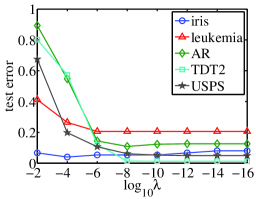
(a) regularization weight $\lambda$

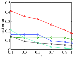
(b) confidence threshold $t$

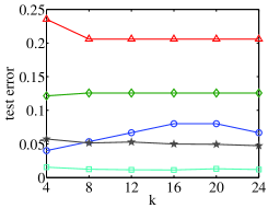
(c) number of neighbors $k$

Figure 1: The influence of the three parameters of nRBFN, $\lambda$, $t$, and $k$, on the classification performance.

7.1.2 nRBFN v.s. Other Classification Algorithms

In this subsection, we compare the classification performance of nRBFN with some other algorithms. The results are shown in Table 1. The involved algorithms include: (1) KNN (k=20), (2) LRC ($\lambda$ is selected via 5-fold cross validation over $10^{\{-13,-12,\dots,-2\}}$), (3) ROLS (regularized orthogonal least squares algorithm for RBFN) [12] (a classical incremental learning method for basis selection, $\lambda$ is selected using the same scheme as nRBFN, $\sigma$ and basis size are provided by nRBFN), (4) RBFNnl (RBFN from Netlab toolbox) [42] (a traditional RBFN that finds the basis via clustering–gaussian mixture model, without regularization, the width of Gaussian is set as the maximum distance between the basis vectors, bias parameters are included, basis size follows nRBFN), (5) nRNwr (nRBFN without regularization, using the same basis as nRBFN), (6) nRNrb (nRBFN with basis chosen randomly from the training set, basis size follows nRBFN), (7) SVM [11] (Gaussian kernel, the weight $C$ is selected over $2^{\{-1,0,\dots,12\}}$ and $\sigma$ is selected over $1.4^{\{-4,-3,\dots,4\}}\times\sigma$ of nRBFN via 5-fold cross validation). Except RBFNnl and SVM, the others are implemented by us using MATLAB.

Table 1: Comparing test error (%) of nRBFN with some algorithms on benchmark data sets. “size” denotes data dimension $\times$ (#training samples + #test samples).

data	size	#classes	KNN	LRC	ROLS	RBFNnl	nRNwr	nRNrb	SVM	nRBFN
iris	4$\times$(75+75)	3	5.3	18.7	4.0	5.3	6.7	5.3	5.3	5.3
wdbc	30$\times$(285+284)	2	6.3	6.3	8.5	4.9	7.7	5.6	4.6	4.9
glass	9$\times$(109+105)	6	39.0	43.8	36.2	67.6	50.5	36.2	31.4	38.1
sonar	60$\times$(105+103)	2	39.8	23.3	18.4	22.3	21.4	18.4	18.4	18.4
wine	13$\times$(90+88)	3	33.0	3.4	1.1	5.7	6.8	1.1	2.3	1.1
colon	2000$\times$(31+31)	2	35.5	16.1	16.1	16.1	16.1	16.1	16.1	16.1
leukemia	7129$\times$(38+34)	2	41.2	17.6	20.6	17.6	20.6	20.6	23.5	20.6
ORL	1024$\times$(200+200)	40	54.0	7.5	8.5	10.0	8.5	8.5	10.0	8.5
AR	1024$\times$(700+700)	100	69.4	6.9	11.3	9.9	12.6	11.3	26.0	11.3
YaleB	1024$\times$(1209+1205)	38	46.1	1.6	1.2	1.5	1.2	1.2	3.2	1.2
TDT2	36771$\times$(4703+4691)	30	1.2	-	-	0.9	98.5	1.0	1.7	1.3
20news	26214$\times$(11314+7532)	20	24.0	-	-	15.0	77.5	14.6	15.1	14.3
USPS	256$\times$(7291+2007)	10	8.2	12.6	-	5.0	5.0	5.2	4.6	4.9
MNIST	784$\times$(60000+10000)	10	3.8	13.4	-	2.0	1.9	2.0	1.5	1.8

The best scores spread across the table. It is hard for a method to dominate over all others on such data sets of diverse nature. However, when we compare them pair-wise, the advantage of nRBFN becomes prominent.

(1) As a linear model, the performance of LRC is limited, as the ideal graph condition implies. It mainly preforms well on high-dimensional data where $p\geq n$, since in this case the rank of row space is full. Results on TDT2 and 20news are absent, since it fails to run on such big data.

(2) The results of nRNwr are inferior to nRBFN, confirming the importance of regularization.

(3) nRBFN generally outperforms ROLS, RBFNnl, and nRNrb, showing the effectiveness of the basis selection strategy of nRBFN. ROLS is resource-consuming, it is unable to run on big data sets. Note that it is hard for RBFNnl and nRNrb themselves to determine a suitable basis size. The strategy of nRBFN, which implicitly controls the size by a user-friendly confidence threshold, makes it much easier.

(4) nRBFN generally obtains better results than SVM on these data sets. Since performance depends on the basis sizes, we list them in Table 3. The support vectors of SVM are found automatically, we note on the first ten smaller data sets, the bases found by nRBFN when setting $t=0.9$ have sizes roughly consistent with those of SVM. It means the basis size has been determined properly according to the complexity of data distribution: when the classes overlap more, more points will be selected as basis, and vice versa. When setting $t=0.9$, most of the uncertain points helpful for determining the classification boundaries have been included. For human face images, it is well-known that the data are clustered according to lightening, expressions, poses, rather than identity. For example, a left lightening cluster may include images from all identities. Thus, almost all points serve as basis. On the four larger sets, the bases obtained by nRBFN are more economical than those of SVM, however, the test error are not necessarily worse.

Table 2: A comparison of the basis sizes of SVM and nRBFN ($t=0.9$). $n$ is the size of training set. “basis (%)” denotes the proportion of the basis vectors with respect to the training set.

data	$n$	basis (%)		test error (%)
		SVM	nRBFN	SVM	nRBFN
iris	75	36.0	42.7	5.3	5.3
wdbc	285	23.2	25.6	4.6	4.9
glass	109	74.3	92.7	31.4	38.1
sonar	105	59.0	100.0	18.4	18.4
wine	90	55.6	82.2	2.3	1.1
colon	31	90.3	100.0	16.1	16.1
leukemia	38	86.8	100.0	23.5	20.6
ORL	200	99.5	100.0	10.0	8.5
AR	700	99.1	100.0	26.0	11.3
YaleB	1209	95.3	100.0	3.2	1.2
TDT2	4703	70.3	27.8	1.7	1.3
20news	11314	79.5	71.7	15.1	14.3
USPS	7291	32.5	19.9	4.6	4.9
MNIST	60000	30.4	14.6	1.5	1.8

Table 3: nRBFN v.s. SVM. nRBFN has the same basis size as SVM. “basis (%)” denotes the proportion of support vectors. The time cost includes the training and testing time.

data	basis(%)	test error (%)		time cost (s)
		SVM	nRBFN	SVM	nRBFN
iris	36.0	5.3	5.3	-	-
wdbc	23.2	4.6	4.9	-	-
glass	74.3	31.4	37.1	-	-
sonar	59.0	18.4	18.4	-	-
wine	55.6	2.3	1.1	-	-
colon	90.3	16.1	16.1	$<$0.1	0.1
leukemia	86.8	23.5	17.6	0.2	0.1
ORL	99.5	10.0	8.0	0.6	0.1
AR	99.1	26.0	11.1	6.7	0.8
YaleB	95.3	3.2	1.4	19.5	1.4
TDT2	70.3	1.7	0.9	77.2	16.5
20news	79.5	15.1	14.3	263.1	82.3
USPS	32.5	4.6	4.7	18.4	24.0
MNIST	30.4	1.5	1.6	1289.1	2455.3

7.1.3 nRBFN v.s. SVM with the Same Basis Size

Next, for a fair comparison between nRBFN and SVM, we let the basis size of nRBFN to be equal to the size of support vectors. This is done by choosing the specific number of samples with the lowest confidence as the basis. The other parameters are set as before. The results are shown in Table 3. In this test, nRBFN performs even better, and the time cost is comparable to that of SVM. Note that, the time cost does not include the part of cross validation. SVM usually needs to run hundreds of times during cross validation, while nRBFN only runs a dozen times.

7.1.4 nRBFN with fixed parameters v.s. SVM

Finally, we test the performance of nRBFN with a fixed set of parameters ($\lambda=10^{-13}$, $t=0.9$, $k=20$). In this case, nRBFN involves no model selection, but the results are still not far from those of SVM, as Table 5 shows.

7.2 Empirical Evaluation of Error and Risk

In this section, we empirically evaluate the fitting error and spectral risk of nRBFN and LRC, and investigate their influence on the performance.

Table 4: SVM v.s. nRBFN with fixed parameters ($\lambda=10^{-13}$, $t=0.9$, $k=20$).

data	SVM	nRBFN
iris	5.3	8.0
wdbc	4.6	5.3
glass	31.4	35.2
sonar	18.4	21.4
wine	2.3	1.1
colon	16.1	16.1
leukemia	23.5	20.6
ORL	10.0	8.5
AR	26.0	12.6
YaleB	3.2	1.2
TDT2	1.7	1.3
20news	15.1	15.2
USPS	4.6	4.9
MNIST	1.5	1.8

Table 5: The effect of regularization in terms of error-and-risk: nRNwr (nRBFN without regularization) v.s. nRBFN. The data sets on which significant changes occur are marked with boldface.

data	$\lambda$	fitting error		spectral risk		test error (%)
		nRNwr	nRBFN	nRNwr	nRBFN	nRNwr	nRBFN
iris	1e-09	1.022	1.044	9.7e+09	2.5e+06	6.7	5.3
wdbc	1e-09	1.045	1.106	2.6e+15	2.4e+06	7.7	4.9
sonar	1e-05	1.000	1.191	1.5e+06	5.5e+03	21.4	18.4
colon	1e-05	1.000	1.001	7.2e+02	6.0e+02	16.1	16.1
leukemia	1e-05	1.000	1.001	1.2e+03	1.0e+03	20.6	20.6
ORL	1e-09	1.000	1.000	5.5e+05	5.4e+05	8.5	8.5
AR	1e-09	1.000	1.014	9.2e+07	2.5e+07	12.6	11.3
YaleB	1e-13	1.000	1.000	1.4e+09	8.2e+08	1.2	1.2
USPS	1e-13	1.056	1.056	4.1e+08	4.1e+08	5.0	4.9
MNIST	1e-13	1.064	1.064	2.4e+10	1.6e+10	1.9	1.8

7.2.1 The Effect of Regularization: nRNwr v.s. nRBFN

We evaluate the effect of regularization through comparing nRNwr (nRBFN without regularization) and nRBFN. The results are shown in Table 5. Due to rank deficiency ($\operatorname{rank}(\tilde{W})<r$), results of nRNwr on glass, wine, TDT2, and 20news are erroneous and not shown. According to the table, on the sets marked with bold face, regularization significantly reduces the spectral risk, mostly by orders of magnitude, while the fitting error is increased slightly, but not yet sacrificed much. On all these sets, the test error have been reduced. This demonstrates the effectiveness of regularization. On the other data sets, regularization affects not much. Since $\lambda$ has been selected for optimal performance, it implies that on these data sets the found row-subspaces by nRNwr probably contain discriminative features rather than noise. Note that, most of these data sets have large sample sizes, indicating sufficient sampling. Even though, regularization does not provide better result in this case, it does not undermine the performance–so long as $\lambda$ is set properly. Considering its capability in dealing with both insufficient and sufficient sampling cases, regularization should be applied.

7.2.2 LRC v.s. nRBFN

We compare the fitting error ($\epsilon$), spectral risk ($\gamma$), the tradeoff ($\epsilon+\lambda\gamma$), and the test error between LRC and nRBFN, and study their influence on the performance. The results are shown in Table 6.

Theoretically, two factors act together contributing to the performance of nRBFN/LRC. One is the rank of basis/data row-space. Despite of the idea graph condition, larger rank implies better fitting capacity. For nRBFN, this can be controlled via $t$. In the extreme case of full rank, zero fitting error can be achieved (although spectral risk is not guaranteed). The other factor is the ideal graph condition. Despite that the rank may be low, so long as the condition is nearly met, both the fitting error and spectral risk will be low.

We analyze Table 6 by two parts. For the data sets from colon to AR, LRC performs equally or better than nRBFN. These data sets are distinct from the others in that the ranks of LRC and nRBFN are exactly the same, and are full. Since both the fitting error and spectral risk depend on the rank, the comparison between LRC and nRBFN is thus fair. The lower test error of LRC can be attributed to the lower spectral risk. Although nRBFN has lower fitting error, it has higher risk of overfitting. Note that, these data sets consist of the gene data and face images. For nRBFN, on these sets all samples are recruited as basis, indicating the classes overlap heavily. Consequently the ideal graph condition will not be met well and the spectral risk can be high. In addition, although the fitting error of LRC seem higher, we found that on these four data sets (plus YaleB) the classification error of both LRC and nRBFN are uniformly zero. All these support the lower test error of LRC.

For the data sets marked with boldface, nRBFN performs better. This can be attributed to the higher ranks and lower fitting error. As to the higher spectral risk, first, the spectral risk is proportionally related to the rank. Second, higher value of spectral risk does not mean error actually happened, but a warning is signalled. The found subspace may be noise or discriminative features. Third, the cross validation determined a much smaller weight to offset the spectral risk, so that the product $\lambda\gamma$ is generally below the magnitude of $10^{-2}$ for nRBFN ($10^{-1}$ for LRC). In contrast to the fitting error that is above 1, the weighted risk is quite small, and the tradeoff $\epsilon+\lambda\gamma\approx\epsilon$. On the one hand, it implies that the performance is overwhelmed by the fitting error. On the other hand, the large offset of nRBFN suggests that the risk warning has been ignored. The cross validation learnt that, after regularization, the warning does no harm, the found subspace was judged to be discriminative features. These analyses also apply to the previous four data sets, since the margins of test error are not large. We conclude nRBFN performs better overall. This is due to the consistently lower fitting error and not severe overfitting.

Table 6: Comparing the fitting error ($\epsilon$), spectral risk ($\gamma$), the tradeoff ($\epsilon+\lambda\gamma$), and the test error between LRC and nRBFN. “rank” denotes the rank of data row-space/basis, divided by $n$. Smaller values are marked with boldface.

data	rank (%)		fitting error ($\epsilon$)		$\lambda$		spectral risk ($\gamma$)		$\epsilon+\lambda\gamma$		test error (%)
	LRC	nRBFN	LRC	nRBFN	LRC	nRBFN	LRC	nRBFN	LRC	nRBFN	LRC	nRBFN
iris	6.7	42.7	1.39	1.04	1e-04	1e-09	9e+00	3e+06	1.39	1.05	18.7	5.3
wdbc	10.9	25.6	3.38	1.11	1e-04	1e-09	1e+03	2e+06	3.49	1.11	6.3	4.9
glass	28.4	92.7	2.09	1.24	1e-04	1e-09	1e+02	2e+07	2.10	1.26	43.8	38.1
sonar	29.5	100.0	1.29	1.19	1e-03	1e-05	5e+01	5e+03	1.33	1.25	23.3	18.4
wine	34.4	82.2	1.10	1.07	1e-08	1e-13	3e+05	1e+11	1.10	1.08	3.4	1.1
colon	100.0	100.0	1.46	1.00	1e-03	1e-05	3e+02	6e+02	1.72	1.01	16.1	16.1
leukemia	100.0	100.0	1.16	1.00	1e-04	1e-05	2e+03	1e+03	1.40	1.01	17.6	20.6
ORL	100.0	100.0	1.44	1.00	1e-04	1e-09	3e+03	5e+05	1.76	1.00	7.5	8.5
AR	100.0	100.0	1.42	1.01	1e-05	1e-09	2e+04	2e+07	1.63	1.04	6.9	11.3
YaleB	84.8	100.0	1.14	1.00	1e-05	1e-13	1e+04	8e+08	1.25	1.00	1.6	1.2
USPS	3.5	19.9	1.42	1.06	1e-04	1e-13	1e+02	4e+08	1.43	1.06	12.6	4.9
MNIST	1.3	14.6	2.15	1.06	1e-03	1e-13	6e+01	2e+10	2.21	1.07	13.4	1.8

7.2.3 How Error and Risk of nRBFN Change as $\lambda$ and $t$ Vary

The setting is the same as Section 7.1.1, now we focus on the fitting error and spectral risk. The results are shown in Figure 2 and Figure 3.

We observe from Figure 2 that: (a) As $\lambda$ decreases, the fitting error steadily decrease. This is as expected. What deserves notice is that the error of the five data sets coincidentally converge at the point $\lambda=10^{-8}$, and reach a plateau of around 1 thereafter. This is consistent with the test error in Figure 1(a). The convergences confirm the law of $\lambda$: as a rule of thumb, setting $\lambda<10^{-8}$ generally delivers near-optimal result of nRBFN. (b) For most data sets, after $\lambda<10^{-12}$, there exists a fairly stable converging range of spectral risk: $10^{8\sim 10}$. This also holds for most other data sets not shown, especially large data sets. The cases of the two gene data are abnormal, they inherently have low spectral risk, variations can be observed only when $\lambda$ becomes large. (c), (d) The weighted spectral risk ($\lambda\gamma$) and its proportion to the tradeoff converge after some points of $\lambda$. They are not comparable to the fitting error.

Next, Figure 3 shows that: (a) As $t$ increases, the fitting error steadily decrease, as expected. At $t=1$, all error converge close to 1, due to full ranks of the similarity matrices. The fitting capacity of nRBFN is a matter of choice. At $t=0.9$, the error have reached a suitable level, so setting $t=0.9$ as the default value meets general situation. (b) We observe that the spectral risk again converges to the range of $10^{8\sim 10}$. The convergences of big data sets are smoother than those of smaller ones. (c), (d) The weighted spectral risk is again not comparable to the fitting error.

It should be noted that the definitions of relative measures are essential, the above laws would disappear, if we simply use the absolute measures.

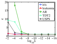
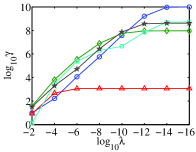
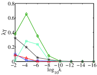
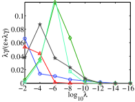
Figure 2: Changes of the error and risk as $\lambda$ varies.

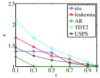
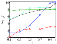
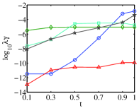
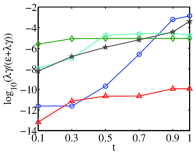
Figure 3: Changes of the error and risk as $t$ varies.

8 Related Work

We discuss the related work of nRBFN, regularization, and generalization error.

1. nRBFN. nRBFN is initially mentioned by [39] and later derived by [59, 60, 67] from probability density estimation and kernel regression. It is also closely related to Gaussian mixture model [63]. Comparing with RBFN, nRBFN has a distinctive feature: in regions far from the samples, the output of RBFN will vanish due to the localized property of radial basis function, while that of nRBFN will not due to the normalization [9]. Consequently, nRBFN provides better smoothness. Meanwhile, the universal approximation capacity is preserved [67, 4]. However, the connection of nRBFN to spectral graph theory is absent before.

2. Regularization. The most classical viewpoint to regularization is from the Bayesian probability, see e.g., [6]. The regularization term corresponds to a prior distribution of the weights, while the error term corresponds to the conditional distribution of the target. However, in the Bayesian view, the effect of regularization on reducing overfitting is not as obvious as the spectral view. Moreover, how to set the regularization weight is unclear, and the uniform case that regularization does not help is not easily observed. Another viewpoint to regularization is from the Tikhonov regularization theory that is based on functional analysis, see e.g., [50]. In this view, the regularization term corresponds to a constraint imposing some smoothness on the approximating function.

3. Generalization error. Even though we are concerned with the generalization problem, this paper is limited to the study of overfitting risk. We did not investigate the problem of generalization error or expected risk. Both of these two concepts relate to the error of the approximating function with respect to the underlying data distribution. In classification application, they indicate the error of a classifier when dealing with new data. Results on this problem had been established both for RBFN [44, 33, 32, 52] and nRBFN [67, 31]. A typical result states that with probability greater than $1-\delta$, the generalization error of RBFN is upper bounded by $O(1/r)+O(\sqrt{(pr\log(nr)-\log\delta)/n})$ [44].

9 Future Work

We mention some limitations of the paper as well as future work worthwhile to do.

Concerning the performance improvements of nRBFN: (1) The relation between the ideal graph condition and the basis selection is not yet investigated. Our motivation to develop the basis selection strategy and parameter setting scheme is to demonstrate the practical performance of nRBFN and provide a baseline algorithm that is easy to use. Searching the optimal basis that is consistent with the theory is an important direction of future work. (2) Optimized or approximated search of nearest neighbors, e.g., [40], can be applied to address the bottleneck of speed improvement. (3) The basis can be further reduced, for there may be many boundary points highly overlapping. (4) Online basis learning can be considered [49], where the basis can be increased, updated, or pruned. It will enable (n)RBFN to handle large scale data.

Concerning the theoretical investigations: (1) The error-and-risk analysis of nRBFN in the perturbation case does not depend on the normality of the columns of similarity matrix. This implies that the analysis can serve as a foundation for the analysis of the other models, e.g., RBFN [52], ELM [27]. Empirically, we found that when RBFN uses our basis selection strategy, it performs similarly to nRBFN and frequently even better. The perturbation analysis in this paper is limited to tiny noise. Extending the analysis from perturbation case to normal noise case has great practical significance. (2) How the two factors of basis size and ideal graph condition interact and contribute to the performance of nRBFN deserves further study. Many of the empirical laws observed in the experiments require explanations. (3) It will be interesting to compare the spectral risk with the VC dimension [64], the error-and-risk tradeoff with the structural risk minimization [64].

Appendix A The Gap between $F$ and the Leading Row-subspace of $\tilde{W}$

Under the ideal graph condition, we know the row-space of $\tilde{W}$ contains $F$. Now we study how much $F$ deviates from the leading row-subspace and when the gap is closed.

For simplicity, we consider one class, since under the ideal graph condition the blocks of matrices of different classes are independent of each other, the largest singular vectors of $\tilde{W}$ consist of the largest singular vectors of each block. We use lower case symbols $w\in\mathbb{R}^{r_{k}\times n_{k}}$, $f$, $x$ to denote the nonzero blocks of the $k$th class. Note, $f$ is a uniform row vector of 1. The deviation can be measured using the idea of the $\ell_{2}$ operator norm [23]:

$$\psi\doteq\max_{y\neq\mathbf{0}}\frac{\|y\tilde{w}\|_{2}^{2}}{\|y\|_{2}^{2}}-\frac{\|x^{*}\tilde{w}\|_{2}^{2}}{\|x^{*}\|_{2}^{2}}\geq 0,$$

On the one hand, by property of the $\ell_{2}$ operator norm, $\max_{y\neq\mathbf{0}}\|y\tilde{w}\|_{2}^{2}/\|y\|_{2}^{2}=\|u_{1}\tilde{w}\|_{2}^{2}/\|u_{1}\|_{2}^{2}=\|\sigma_{1}v_{1}\|_{2}^{2}/\|u_{1}\|_{2}^{2}=\sigma_{1}^{2}$, where $u_{1}$, $v_{1}$, and $\sigma_{1}$ denote the largest singular vectors and value of $\tilde{w}$. On the other hand, by Proposition 4, $x^{*}$ is a uniform row vector of 1, and $x^{*}\tilde{w}=f$. Thus,

$$\psi=\sigma_{1}^{2}-n_{k}/r_{k}.$$

$\psi=0$ if and only if $\sigma_{1}^{2}=n_{k}/r_{k}$, i.e., $x^{*}$ and $f$ become the largest singular vectors. The remaining effort focuses on the estimation of $\sigma_{1}$. We have the following proposition:

Proposition 20.

For any nonnegative matrix $\tilde{w}\in\mathbb{R}^{r_{k}\times n_{k}}$ $(r_{k}\leq n_{k})$ with each column sum normalized to 1, assume $\tilde{w}$ is of full rank, then

1. $n_{k}/r_{k}\leq\sigma_{1}^{2}\leq z_{max}$, where $z_{max}$ is the maximal row sum of $\tilde{w}$.

2. $n_{k}/r_{k}=\sigma_{1}^{2}$ if and only if the row sums are even, i.e., $z_{max}=n_{k}/r_{k}$.

Proof.

1) The problem is resolved with the help of a closely related matrix, $\hat{W}\doteq Z^{-\frac{1}{2}}\tilde{W}$, where $Z$ is a diagonal matrix of the row sums of $\tilde{W}$. $\hat{W}$ is the component of a reduced Laplacian matrix, $\hat{L}\doteq I-\hat{W}^{T}\hat{W}$, that is also for dealing with the scalable problem of large graph construction [37]. Under the ideal graph condition, $\tilde{W}$ is block-wise, so is the reduced similarity matrix $\hat{W}^{T}\hat{W}$, which implies $\hat{W}^{T}\hat{W}$ is ideal too. Therefore, $F$ is the smallest eigenvectors of $\hat{L}$ (eigenvalue 0), and equivalently, the largest right singular vectors of $Z^{-\frac{1}{2}}\tilde{W}$ (singular value 1). Denote $\hat{w}$ and $z$ to be the corresponding blocks of class $k$. We have

$$\sigma_{1}^{2}=\sup_{y\neq\mathbf{0}}\frac{\|y\tilde{w}\|_{2}^{2}}{\|y\|_{2}^{2}}=\sup_{y\neq\mathbf{0}}\frac{\|yz^{\frac{1}{2}}\hat{w}\|_{2}^{2}}{\|y\|_{2}^{2}}.$$

Denote $y^{\prime}=yz^{\frac{1}{2}}$, it turns into

$$\sigma_{1}^{2}=\sup_{y^{\prime}\neq\mathbf{0}}\frac{\|y^{\prime}\hat{w}\|_{2}^{2}}{\|y^{\prime}z^{-\frac{1}{2}}\|_{2}^{2}}\leq\sup_{y^{\prime}\neq\mathbf{0}}\frac{\|y^{\prime}\hat{w}\|_{2}^{2}}{z_{max}^{-1}\|y^{\prime}\|_{2}^{2}}\leq z_{max}.$$

$z_{max}\doteq\max_{i}z_{ii}$. In the last inequality, we have used the fact that the largest singular value of $\hat{w}$ is 1.

2) First, note that $n_{k}/r_{k}$ is also the mean of the row sums of $\tilde{w}$, since the sum of row sums is equal to the sum of column sums, which is $n_{k}$. Thus, if the row sums are even, then $z_{max}=n_{k}/r_{k}$. Consequently $n_{k}/r_{k}=\sigma_{1}^{2}$. Conversely, if $n_{k}/r_{k}=\sigma_{1}^{2}$, then it means $x^{*}$ and $f$ are the largest singular vectors, since $\|x^{*}\tilde{w}\|_{2}^{2}/\|x^{*}\|_{2}^{2}=n_{k}/r_{k}$. In this case, again by the property of operator norm,

$$\sigma_{1}^{2}=\frac{\|\tilde{w}f\|_{2}^{2}}{\|f\|_{2}^{2}}=\frac{\sum_{i}z_{ii}^{2}}{n_{k}}\geq\frac{(\sum_{i}z_{ii})^{2}/r_{k}}{n_{k}}=\frac{n_{k}}{r_{k}}.$$

The equality holds, if and only if $z_{ii}$’s are even. ∎

With this proposition, we immediately have

Proposition 21.

$$\psi\leq z_{max}-n_{k}/r_{k}.$$

$\psi=0$ if and only if the row sums are even, i.e., $z_{max}=n_{k}/r_{k}$.

By this proposition, we finally arrive at Theorem 5.

References

- [1] Michal Aharon, Michael Elad, and Alfred Bruckstein. K-SVD: An algorithm for designing overcomplete dictionaries for sparse representation. IEEE Transactions on Signal Processing, 54(11):4311–4322, 2006.
- [2] Mikhail Belkin and Partha Niyogi. Laplacian eigenmaps for dimensionality reduction and data representation. Neural Computation, 15(6):1373–1396, 2003.
- [3] Mikhail Belkin, Partha Niyogi, and Vikas Sindhwani. Manifold regularization: A geometric framework for learning from labeled and unlabeled examples. Journal of Machine Learning Research, 7(3):2399–2434, 2006.
- [4] M Benaim. On functional approximation with normalized gaussian units. Neural Computation, 6(2):319–333, 1994.
- [5] Christopher M Bishop. Improving the generalization properties of radial basis function neural networks. Neural Computation, 3(4):579 – 588, 1991.
- [6] Christopher M Bishop. Pattern Recognition and Machine Learning. Springer New York, 2006.
- [7] Enrico Blanzieri. Theoretical interpretations and applications of radial basis function networks. Technical Report No. DIT-03-023, 2003.
- [8] D. S Broomhead and David Lowe. Multivariable functional interpolation and adaptive networks. Complex Systems, 2(3):321–355, 1988.
- [9] Guido Bugmann. Normalized gaussian radial basis function networks. Neurocomputing, 20(1 C3):97–110, 1998.
- [10] Pak K Chan, Martine DF Schlag, and Jason Y Zien. Spectral k-way ratio-cut partitioning and clustering. IEEE Transactions on Computer-Aided Design of Integrated Circuits and Systems, 13(9):1088–1096, 1994.
- [11] Chih Chung Chang and Chih Jen Lin. Libsvm: a library for support vector machines. Acm Transactions on Intelligent Systems and Technology, 2:27:1–27:27, 2011.
- [12] S. Chen, E. S. Chng, and K. Alkadhimi. Regularized orthogonal least squares algorithm for constructing radial basis function networks. International Journal of Control, 64(5):829–837, 1996.
- [13] S Chen, C.F.N Cowan, and P.M Grant. Orthogonal least squares learning algorithm for radial basis function networks. IEEE Transactions on Neural Networks, 2(2):302 – 309, 1991.
- [14] Fan RK Chung. Spectral Graph Theory. American Mathematical Society, 1997.
- [15] Corinna Cortes and Vladimir Vapnik. Support-vector networks. Machine Learning, 20(3):273–297, 1995.
- [16] Trevor F Cox and Michael AA Cox. Multidimensional scaling. Chapman and Hall, 2001.
- [17] III David Bau and Lloyd N. Trefethen. Numerical Linear Algebra. SIAM, 1997.
- [18] Kelin Du and M. N. S. Swamy. Neural Networks and Statistical Learning. Springer London, 2014.
- [19] Michael Elad. Sparse and Redundant Representations: From Theory to Applications in Signal and Image Processing. Springer, 2010.
- [20] Ehsan Elhamifar and Rene Vidal. Sparse subspace clustering: Algorithm, theory, and applications. IEEE Transactions on Pattern Analysis and Machine Intelligence, 35(11):2765–2781, 2013.
- [21] K. Engan, S. O. Aase, and J. Hakon Husoy. Method of optimal directions for frame design. In IEEE International Conference on Acoustics, Speech, and Signal Processing, volume 5, pages 2443–2446, 1999.
- [22] Manuel Fernández-Delgado, Eva Cernadas, Senán Barro, and Dinani Amorim. Do we need hundreds of classifiers to solve real world classification problems? Journal of Machine Learning Research, 15(1):3133–3181, 2014.
- [23] G.H. Golub and C.F. Van Loan. Matrix Computations. Johns Hopkins University Press, 1996.
- [24] Xiaofei He and Partha Niyogi. Locality preserving projections. In Advances in Neural Information Processing Systems, volume 16, page 153. MIT Press, 2004.
- [25] Zhenfang Hu, Gang Pan, Yueming Wang, and Zhaohui Wu. Spectral sparse representation for clustering: Evolved from pca, k-means, laplacian eigenmap, and ratio cut. Eprint Arxiv, 2014.
- [26] Guang-Bin Huang, P Saratchandran, and Narasimhan Sundararajan. An efficient sequential learning algorithm for growing and pruning rbf (gap-rbf) networks. IEEE Transactions on Systems, Man, and Cybernetics, 34(6):2284–2292, 2004.
- [27] Guang Bin Huang, Qin Yu Zhu, and Chee Kheong Siew. Extreme learning machine: Theory and applications. Neurocomputing, 70(1-3):489–501, 2006.
- [28] IT Jolliffe. Principal Component Analysis. Springer, 2002.
- [29] Sepandar D. Kamvar, Klein Dan, and Christopher D. Manning. Spectral learning. International Joint Conference on Artificial Intelligence, pages 561–566, 2003.
- [30] N. B. Karayiannis. Reformulated radial basis neural networks trained by gradient descent. IEEE Transactions on Neural Networks, 10(3):657–671, 1999.
- [31] B Kegl, A Krzyżak, and H Niemann. Radial basis function networks and complexity regularization in function learning and classification. In International Conference on Pattern Recognition, pages 81–86, 2000.
- [32] A Krzyżak and T Linder. Radial basis function networks and complexity regularization in function learning. IEEE Transactions on Neural Networks, 9(2):247–256, 1998.
- [33] A Krzyżak, T Linder, and C Lugosi. Nonparametric estimation and classification using radial basis function nets and empirical risk minimization. IEEE Transactions on Neural Networks, 7(2):475–87, 1996.
- [34] Brian Kulis, Sugato Basu, Inderjit Dhillon, and Raymond Mooney. Semi-supervised graph clustering: a kernel approach. In International conference on Machine learning, pages 457–464, 2005.
- [35] M. Lichman. UCI machine learning repository, 2013.
- [36] Guangcan Liu, Zhouchen Lin, Shuicheng Yan, Ju Sun, Yong Yu, and Yi Ma. Robust recovery of subspace structures by low-rank representation. IEEE Transactions on Pattern Analysis and Machine Intelligence, 35(1):171–184, 2013.
- [37] Wei Liu, Junfeng He, and Shih Fu Chang. Large graph construction for scalable semi-supervised learning. In International Conference on Machine Learning, pages 679–686, 2010.
- [38] James MacQueen. Some methods for classification and analysis of multivariate observations. In Proceedings of the Fifth Berkeley Symposium on Mathematical Statistics and Probability, pages 281–297, 1967.
- [39] John Moody and Christian J. Darken. Fast learning in networks of locally-tuned processing units. Neural Computation, 1:281–294, 1989.
- [40] Marius Muja and David G. Lowe. Scalable nearest neighbor algorithms for high dimensional data. IEEE Transactions on Pattern Analysis and Machine Intelligence, 36(11):2227, 2014.
- [41] M. T. Musavi, W. Ahmed, K. H. Chan, K. B. Faris, and D. M. Hummels. On the training of radial basis function classifiers. Neural Networks, 5(05):595–603, 1992.
- [42] Ian T. Nabney. Netlab: Algorithms for Pattern Recognition. Springer Berlin, 2003.
- [43] Andrew Y Ng, Michael I Jordan, and Yair Weiss. On spectral clustering: analysis and an algorithm. Advances in Neural Information Processing Systems, 2:849–856, 2002.
- [44] P Niyogi and F Girosi. On the relationship between generalization error, hypothesis complexity, and sample complexity for radial basis functions. Neural Computation, 8(4):819–842, 1996.
- [45] Bruno A. Olshausen and David J. Field. Emergence of simple-cell receptive field properties by learning a sparse code for natural images. Nature, 381(6583):607–609, 1996.
- [46] Mark J. L. Orr. Regularization in the selection of radial basis function centers. Neural Computation, 7(3):606–623, 1995.
- [47] Yen Jen Oyang, Shien Ching Hwang, Yu Yen Ou, Chien Yu Chen, and Zhi Wei Chen. Data classification with radial basis function networks based on a novel kernel density estimation algorithm. IEEE Transactions on Neural Networks, 16(1):225 – 236, 2005.
- [48] J Park and I Sandberg. Universal approximation using radial-basis-function networks. Neural Computation, 3(2):246–257, 1991.
- [49] John Platt. A resource-allocating network for function interpolation. Neural Computation, 3(2):213–225, 1991.
- [50] T. Poggio and F. Girosi. Networks for approximation and learning. Proceedings of the IEEE, 78(9):1481–1497, 1990.
- [51] M. J. D. Powell. Radial basis functions for multivariable interpolation: a review. Algorithms for Approximation, pages 143–167, 1987.
- [52] Qichao Que and Mikhail Belkin. Back to the future: radial basis function networks revisited. International Conference on Artificial Intelligence and Statistics, page 1375 C1383, 2016.
- [53] Ryan Rifkin and Aldebaro Klautau. In defense of one-vs-all classification. Journal of Machine Learning Research, 5(1):101–141, 2004.
- [54] Sam T Roweis and Lawrence K Saul. Nonlinear dimensionality reduction by locally linear embedding. Science, 290(5500):2323–2326, 2000.
- [55] B. Schölkopf, K. Sung, C. Burges, F. Girosi, P. Niyogi, T. Poggio, and V. Vapnik. Comparing support vector machines with gaussian kernels to radial basis function classifiers. IEEE Transactions on Signal Processing, 45(11):2758–2765, 1997.
- [56] Bernhard Schölkopf, Alexander Smola, and Klaus-Robert Müller. Nonlinear component analysis as a kernel eigenvalue problem. Neural Computation, 10(5):1299–1319, 1998.
- [57] Friedhelm Schwenker, Hans A. Kestler, and Günther Palm. Three learning phases for radial-basis-function networks. Neural Networks, 14(4 C5):439–458, 2001.
- [58] Jianbo Shi and Jitendra Malik. Normalized cuts and image segmentation. IEEE Transactions on Pattern Analysis and Machine Intelligence, 22(8):888–905, 2000.
- [59] Donald F. Specht. Probabilistic neural networks. Neural Networks, 3(1):109–118, 1990.
- [60] Donald F. Specht. A general regression neural network. IEEE Transactions on Neural Networks, 2(6):568–576, 1991.
- [61] G. W. Stewart and Ji Guang Sun. Matrix Perturbation Theory. Academic Press, 1990.
- [62] Joshua B Tenenbaum, Vin De Silva, and John C Langford. A global geometric framework for nonlinear dimensionality reduction. Science, 290(5500):2319–2323, 2000.
- [63] Volker Tresp, Jürgen Hollatz, and Subutai Ahmad. Network structuring and training using rule-based knowledge. In Advances in Neural Information Processing Systems, pages 871–878, 1993.
- [64] Vladimir N. Vapnik. The Nature of Statistical Learning Theory. Springer, 2000.
- [65] Ulrike Von Luxburg. A tutorial on spectral clustering. Statistics and Computing, 17(4):395–416, 2007.
- [66] Tiantian Xie, Yu Hao, J. Hewlett, P. Rozycki, and B. Wilamowski. Fast and efficient second-order method for training radial basis function networks. IEEE Transactions on Neural Networks and Learning Systems, 23(4):609–619, 2012.
- [67] Lei Xu, Adam Krzyżak, and Alan Yuille. On radial basis function nets and kernel regression: Statistical consistency, convergence rates, and receptive field size. Neural Networks, 7(4):609–628, 1994.
- [68] Jieping Ye. Least squares linear discriminant analysis. International Conference on Machine Learning, 3(10):1087–1093, 2007.
- [69] H. Yu, P. D. Reiner, T. Xie, T Bartczak, and B. M. Wilamowski. An incremental design of radial basis function networks. IEEE Transactions on Neural Networks and Learning Systems, 25(10):1793–1803, 2014.
- [70] Dengyong Zhou, Olivier Bousquet, Thomas Navin Lal, Jason Weston, and Bernhard Schölkopf. Learning with local and global consistency. Advances in Neural Information Processing Systems, 17(4):321–328, 2004.
- [71] Xiaojin Zhu. Semi-supervised learning literature survey. Computer Science, 37(1):63–77, 2008.
- [72] Xiaojin Zhu, Zoubin Ghahramani, and John D. Lafferty. Semi-supervised learning using gaussian fields and harmonic functions. International Conference on Machine Learning, pages 912–919, 2003.