Local risk-minimization with multiple assets under illiquidity with applications in energy markets

Abstract

We propose a hedging approach for general contingent claims when liquidity is a concern and trading is subject to transaction cost. Multiple assets with different liquidity levels are available for hedging. Our risk criterion targets a tradeoff between minimizing the risk against fluctuations in the stock price and incurring low liquidity costs. Following Çetin et al. (2004) we work in an arbitrage-free setting assuming a supply curve for each asset. In discrete time, following the ideas in Schweizer et. al. (Schweizer, 1988; Lamberton et al., 1998) we prove the existence of a locally risk-minimizing strategy under mild conditions on the price process. Under stochastic and time-dependent liquidity risk we give a closed-form solution for an optimal strategy in the case of a linear supply curve model. Finally we show how our hedging method can be applied in energy markets where futures with different maturities are available for trading. The futures closest to their delivery period are usually the most liquid but depending on the contingent claim not necessary optimal in terms of hedging. In a simulation study we investigate this tradeoff and compare the resulting hedge strategies with the classical ones.

JEL Classification: G11, G13, C61

Keywords: local risk-minimization, quadratic hedging, liquidity cost, energy markets, multiple assets

1 Introduction

In this paper we deal with the problem of hedging general contingent claims under illiquidity. Stochastic liquidity cost is incurred by hedging with multiple assets with possibly different levels of liquidity. Our main motivation comes from energy markets. Consider for example an agent hedging an Asian-style call option written on the average spot price $S=(S_{u})_{0\leq u\leq T_{2}}$ of energy. Such an option has the payoff

$$\left(\frac{1}{T_{2}-T_{1}}\int_{T_{1}}^{T_{2}}S_{u}du-K\right)^{+}$$ (1)

for a strike $K$, with a so-called delivery period $[T_{1},T_{2}]$. The instruments available for hedging such options are futures delivering over the same or a different time period. Hedging is a challenge though since these futures are either not trading in their delivery period at all (such a setting was considered in Benth & Detering, 2015) or are very illiquid such that hedging incurs large transaction costs. In addition, futures are usually very illiquid for $t\ll T_{1}$, so their liquidity has a delicate time-structure. In the market, multiple futures with different delivery periods (week, month, quarter, year) and different levels of liquidity are available as hedging instruments. The results of our paper can be applied to hedging options in energy markets with multiple futures by accounting for their different levels of liquidity. The Asian-style option is a particular example but other payoffs as for example Quanto options (see Benth et al., 2015) can be handle d equally.

The effect of illiquidity on hedging and optimal trading is a very active research topic in mathematical finance. Still, there is neither an agreed notion of liquidity risk, which is roughly speaking the additional risk due to timing and size of a trade, nor a standard approach for hedging under liquidity costs. A good overview on existing liquidity models in continuous and discrete time can be found in Gökay et al. (2011).

There are basically two different approaches how to model liquidity risk. The first one is a class of models incorporating feedback effects, that is when the trade volume has a lasting impact on the asset price (see e.g. Bank & Baum, 2004), also known as permanent price impact or lasting impact. The second approach considers smaller agents whose transactions have no lasting impact on the price of the underlying (see e.g. Çetin et al., 2004, and the references therein).

In this paper we stay within the small agents approach and understand liquidity costs as the transaction costs incurred from the hedging strategy by trading through a fast recovering limit order book. In particular we follow the arbitrage-free model suggested by Çetin et al. (2004), who introduced the so called supply curve model. There, the asset price is a function of the trade size and the authors developed an extended arbitrage pricing theory.

In addition to the vast majority of papers on illiquid markets dealing with optimal execution, there are also many papers investigating hedging under illiquidity, most of them consider super-replication (see for example Bank & Baum, 2004; Çetin et al., 2010; Gökay & Soner, 2012). As super-replication is often too expensive we use a quadratic risk criterion. In the classical frictionless theory without transaction costs, there are two main approaches for quadratic hedging (see Schweizer, 2001, for a survey). First, the mean-variance approach, which was introduced in Föllmer & Sondermann (1986), relies on self-financing strategies which produce as final outcome the portfolio $V_{T}:=c+\int_{0}^{T}X_{u}dS_{u}$ for some initial capital $c\in\mathbb{R}$ and a trading strategy $X$ in the risky asset $S=(S_{u})_{0\leq u\leq T}$. The goal of this method is to look for the best approximation of a contingent claim $H$ by the terminal portfolio value $V_{T}$, that is minimizing the quadratic hedge error

$${\mathbb{E}}\left[\left(H-\left(c+\int_{0}^{T}X_{u}dS_{u}\right)\right)^{2}\right]$$ (2)

under the real world probability measure and over an appropriately constrained set of strategies. This is also called global risk-minimization. In discrete time, this problem was solved in Schweizer (1995) in a general setting and relaxing the assumptions imposed earlier in Schäl (1994). Later on, this was extended to the multidimensional case with proportional transaction cost in Motoczyński (2000) and Beutner (2007) where the authors show existence of an optimal strategy. The papers Rogers & Singh (2010), Agliardi & Gençay (2014) and Bank et al. (2017) can be seen as an extension under illiquidity of the mean-variance hedging criterion, which is based on minimizing the global risk against random fluctuations of the stock price incurring low liquidity costs.

A second quadratic method for hedging in an incomplete market is local risk-minimization first introduced in Schweizer (1988) and later extended in Lamberton et al. (1998) by accounting for proportional transaction costs in the discrete time case. For discrete time $k=0,\dots,T$ this method does not insist on the self-financing condition but instead the goal is to find a strategy $(X,Y)=(X_{k+1},Y_{k})_{k=0,\dots,T}$ with book value $V_{k}=X_{k+1}S_{k}+Y_{k}$ (the risk-free asset is assumed constantly equal to $1$) such that $H=V_{T}$, the cost process $C_{k}=V_{k}-\sum_{m=1}^{k}X_{m}(S_{m}-S_{m-1})$ is a martingale and the variance of the incremental cost is minimized. Here, the strategy $X_{k+1}$ represents the number of shares held in the risky asset and $Y_{k}$ the units held in the bank account in the time interval $(k,k+1]$. In our paper, we extend the work of Schweizer (1988) by considering a multidimensional asset pri ce process in discrete time. Secondly we extend the local risk-minimizing quadratic criterion to an illiquid market in the spirit of Rogers & Singh (2010) and Agliardi & Gençay (2014).

In contrast to the existing literature our approach and setting is designed to address the above mentioned problem in energy markets. For this we need a multi-dimensional setup to allow for hedging with multiple futures. Second, the assets price dynamics has to be general enough to capture the characteristics of energy markets and we need a time dependent liquidity structure. Our risk criterion is chosen such that it allows for more explicit formulas for the optimal strategy than existing approaches. Furthermore, as shown in a case study, they are also computationally tractable. Our main result is the existence of a locally risk-minimizing strategy under illiquidity requiring only mild conditions on the asset price. These conditions are quite technical but they can be reduced to conditions on the covariance matrix of the price process, which can be checked easily for most processes relevant in practice. Furthermore, the strategies can be calculated backwards in time by using a least-squares Monte Carlo algorithm.

Our setup allows us to explore the tradeoff between liquidity and hedge quality of available hedge instruments. For example, consider the Asian-style option (1) in a market where different futures with different delivery periods and different liquidity levels are available for hedging. In such a situation, there are futures with delivery period well matching the delivery period of the option payout resulting in a strong correlation between the future and the option to hedge. However, in certain time periods these hedge-optimal futures are very illiquid and futures which are less correlated but more liquid might be better for hedging. Our framework allows us to explore this tradeoff and provide market-makers with a more profound tool for risk management.

The paper is structured as follows. Section 2 explains the model framework and describes the basic problem. In Section 3 we focus on a linear supply curve and impose necessary assumptions on the price process to prove our main existence Theorem 3.10. Sufficient conditions to check the assumptions are also provided. Section 4 considers an application to energy markets. Optimal strategies under illiquidity are simulated by means of a least-squares Monte Carlo method. This allows us to explore the tradeoff between liquidity and hedging performance of futures available for hedging.

2 The Model

Given a filtered probability space $(\Omega,\mathcal{F},\mathbb{F},\mathbb{P})$ consider a financial market consisting of $d+1$ assets. We denote by $\mathbb{P}$ the objective probability measure and by $\mathbb{F}$ the filtration $\mathbb{F}=(\mathcal{F}_{k})_{k=0,1,\dots,T}$, which describes the flow of information. We shall use the indices $k=0,1,\dots,T$ to refer to a discrete time grid with time points $t_{0}<t_{1}<\dots<t_{T}$ and sometimes use both interchangeably. An $\mathbb{F}$-adapted, nonnegative $d$-dimensional stochastic process $S=(S_{k})_{k=0,1,\dots,T}$ describes the discounted price of $d$ risky assets (typically futures or stocks). We use $S_{k}^{j}$ to refer to the price of asset $j$ at time $t_{k}$. Furthermore, a riskless asset (typically a bond) exists whose discounted price is constantly $1$.

Similar as in Çetin et al. (2004) we assume that a hedger observes an exogenously given nonnegative $d$-dimensional supply curve $S_{k}(x)$ where $S_{k}(x)^{j}:=S_{k}^{j}(x^{j})$ represents the $j$-th stock price per share at time $k$ for the purchase (if $x^{j}>0$) or sale (if $x^{j}<0$) of $|x^{j}|$ shares. We call $S(0)=S$ the marginal price. The supply curve determines the actual price that market participants pay or receive respectively for a transaction of size $x$ at time $k$. This curve is also assumed to be independent of the participants past actions which implies no lasting impact of the trading strategy on the supply curve. The only assumption that we need for the moment is measurability of the supply curve w.r.t. the filtration $\mathbb{F}$ and that it is non-decreasing in the number of shares $x$, i.e. for each $k$ and $j$, $S_{k}(x)^{j}\leq S_{k}(y)^{j},\,\mathbb{P}-a.s.$ for $x^{j}\leq y^{j}$. This will ensure that the liquidity costs are non-negative.

In Çetin et al. (2004) the authors develop a continuous time version of such a supply curve model and an extended arbitrage pricing theory. They show that the existence of an equivalent local martingale measure $\mathbb{Q}$ for the marginal price process $S$ rules out arbitrage. A similar results can easily be seen to hold in our setting as liquidity cost is always positive.

However, even a unique martingale measure (and state space restrictions in a discrete setting) do not necessarily ensure completeness if one incorporates illiquidity. Since we cannot hedge perfectly, we want to minimize locally the risk of hedging under illiquidity according to an optimality criterion introduced in Definition 2.3.

In the following we shall consider an investor who aims at hedging an $\mathcal{F}_{T}$-measurable claim $H$. For $x\in\mathbb{R}^{d}$, let $\left\lvert x\right\rvert$ denote the Euclidian norm and $x^{*}$ the transpose of $x$. Further, $\langle x,y\rangle$ denotes the inner product of $x,y\in\mathbb{R}^{d}$. Adapting Schweizer (1988) we define the investor’s possible trading strategies. For this we denote by $\mathbb{L}_{T}^{p}(\mathbb{R}^{d})$ (in short $\mathbb{L}_{T}^{p,d}$), the space of all $\mathcal{F}_{T}$-measurable random variables $Z:\Omega\to\mathbb{R}^{d}$ satisfying $\lVert Z\rVert^{p}=\mathbb{E}(\left\lvert Z\right\rvert^{p})<\infty$. We abbreviate $\Delta S_{k}:=S_{k}-S_{k-1}$. Furthermore, we denote by $\Theta_{d}(S)$ the space of all $\mathbb{R}^{d}$-valued predictable strategies $X=(X_{k})_{k=1,2,\dots,T+1}$ so that $X_{k}^{*}\Delta S_{k}\in\mathbb{L}_{T}^{2,1}$ and $\Delta X_{k+1}^{*}[S_{k}(\Delta X_{k+1})-S_{k}(0)]\in\mathbb{L}_{T}^{1,1}$ for $k=1,2,\dots,T$.

Definition 2.1.

A pair $\varphi=(X,Y)$ is called a trading strategy if:

1. $Y=(Y_{k})_{k=0,1,\dots,T}$ is a real-valued $\mathbb{F}$-adapted process.

2. $X\in\Theta_{d}(S)$.

3. $V_{k}(\varphi):=X_{k+1}^{*}S_{k}+Y_{k}\in\mathbb{L}_{T}^{2,1}$ for $k=0,1,\dots,T$.

We call $V_{k}(\varphi)$ the marked-to-market value or the book value of the portfolio $(X_{k+1},Y_{k})$ at time $k$. We interpret $X_{k+1}^{j}$ as the number of shares held in the risky asset $S_{k}^{j}$ and $Y_{k}$ the units held in the riskless asset (bank account) in the time interval $(k,k+1]$. Note that with a non-flat supply curve, there is no unique value for a portfolio, as the value that can be realized depends on the liquidation strategy.

2.1 Cost And Risk process

Consider an $\mathbb{L}_{T}^{2,1}$-contingent claim of the form $H=\bar{X}_{T+1}^{*}S_{T}+\bar{Y}_{T}$, where $\bar{X}_{T+1}^{*}S_{T}\in\mathbb{L}_{T}^{2,1}$, $\bar{X}_{T+1}\in\mathbb{L}_{T}^{2,d}$ and the components of the pair $(\bar{X}_{T+1},\bar{Y}_{T})$ are $\mathcal{F}_{T}$-measurable random variables describing the quantity in risky assets and bonds respectively that the option seller is committed to provide to the buyer at the expiration date $T$ of the financial contract $H$.

Assuming that at time $k\in\{1,2,\dots,T\}$ an order of $\Delta Y_{k}:=Y_{k}-Y_{k-1}$ bonds and $\Delta X_{k+1}:=X_{k+1}-X_{k}$ shares is made, then the total outlay (under liquidity costs) is

$$\Delta Y_{k}+\Delta X_{k+1}^{*}S_{k}(\Delta X_{k+1})=\Delta Y_{k}+\Delta X_{k+1}^{*}S_{k}+\Delta X_{k+1}^{*}[S_{k}(\Delta X_{k+1})-S_{k}(0)].$$ (3)

Note that $S_{k}(0)=S_{k}$ is the marginal price, such that the last term can be seen as the transaction cost resulting from market illiquidity. Furthermore, using the definition of the book value the previous equation can be written as

$$\Delta Y_{k}+\Delta X_{k+1}^{*}S_{k}(\Delta X_{k+1})=\Delta V_{k}(\varphi)-X_{k}^{*}\Delta S_{k}+\Delta X_{k+1}^{*}[S_{k}(\Delta X_{k+1})-S_{k}(0)]$$ (4)

For a self-financing trading strategy the total outlay at time $k$ would be zero.

Now, by defining $\hat{C}_{0}(\varphi):=V_{0}(\varphi)$, the initial cost, we can define the cost process under illiquidity $\hat{C}(\varphi)=(\hat{C}_{k}(\varphi))_{k=0,1,\dots,T}$ as

$$\hat{C}_{k}(\varphi):=\sum_{m=1}^{k}\Delta Y_{m}+\sum_{m=1}^{k}\Delta X_{m+1}^{*}S_{m}(\Delta X_{m+1})+V_{0}(\varphi).$$ (5)

It quantifies the cumulative costs of the strategy $\varphi=(X,Y)$. A simple calculation using the definition of $V_{k}(\varphi)$ shows that

$$\hat{C}_{k}(\varphi)=V_{k}(\varphi)-\sum_{m=1}^{k}X_{m}^{*}\Delta S_{m}+\sum_{m=1}^{k}\Delta X_{m+1}^{*}[S_{m}(\Delta X_{m+1})-S_{m}(0)],$$ (6)

which will be needed later. If we can ensure that the cost process is square integrable, then we can define the quadratic risk process under illiquidity $\hat{R}(\varphi)=(\hat{R}_{k}(\varphi))_{k=0,1,\dots,T}$ by

$$\hat{R}_{k}(\varphi):=\mathbb{E}[(\hat{C}_{T}(\varphi)-\hat{C}_{k}(\varphi))^{2}|\mathcal{F}_{k}]\,.$$ (7)

At this point we would like to mention that the classical local risk-minimization approach aims at finding a locally risk-minimizing strategy $\varphi=(X,Y)$ such that $V_{T}(\varphi)=H$ with $X_{T+1}=\bar{X}_{T+1}$ and $Y_{T}=\bar{Y}_{T}$ (see Section 2.2 for more details).

We denote by $C(\varphi)=(C_{k}(\varphi))_{k=0,1,\dots,T}$ the classical cost process without liquidity costs (i.e., $S(x)=S(0)$), that is

$$C_{k}(\varphi):=V_{k}(\varphi)-\sum_{m=1}^{k}X_{m}^{*}\Delta S_{m},$$ (8)

and obtain the relation

$$\hat{C}_{T}(\varphi)-\hat{C}_{k}(\varphi)=C_{T}(\varphi)-C_{k}(\varphi)+\sum_{m=k+1}^{T}\Delta X_{m+1}^{*}[S_{m}(\Delta X_{m+1})-S_{m}(0)].$$ (9)

Furthermore, we denote by $R(\varphi)=(R_{k}(\varphi))_{k=0,1,\dots,T}$ the classical risk process, defined as in (7) but with $\hat{C}$ replaced by $C$.

One could also define the linear risk process under illiquidity

$$\bar{R}_{k}(\varphi):=\mathbb{E}[|\hat{C}_{T}(\varphi)-\hat{C}_{k}(\varphi)||\mathcal{F}_{k}]$$ (10)

which is motivated in Coleman et al. (2003).

Remark 2.1.

A linear local risk-minimization criterion might be more natural than a quadratic one from a financial perspective. The $L^{2}$-norm overemphasizes large values even if these values occur with small probability. Nevertheless, by minimizing over the $L^{2}$-norm, it is possible to get explicit results.

A combination of the two, that means measuring the quadratic difference of the classical cost process and linearly the liquidity costs, yields the quadratic-linear risk process under illiquidity.

$$T_{k}(\varphi):=\mathbb{E}[(C_{T}(\varphi)-C_{k}(\varphi))^{2}|\mathcal{F}_{k}]+\mathbb{E}[\sum_{m=k+1}^{T}\Delta X_{m+1}^{*}[S_{m}(\Delta X_{m+1})-S_{m}(0)]|\mathcal{F}_{k}].$$ (11)

As we will see later on, by minimizing the expression in (11) we will be able to construct an explicit representation of the LRM-strategy under illiquidity where large values of liquidity costs are not overemphasized by the $L^{2}$-norm.

2.2 Description of the basic problem

The aim of the classical local risk-minimization is to minimize locally the conditional mean square incremental cost of a strategy. Our criterion is targeting on minimizing locally the risk against random fluctuations of the stock price but at the same time reducing liquidity costs. It balances low liquidity costs against poor replication. Such an approach is similar to Agliardi & Gençay (2014) or Rogers & Singh (2010) and yields a tractable problem.

In minimizing locally the risk process at time $k$, we only minimize in $Y_{k}$ and $X_{k+1}$ in order to make the current optimal choice of the strategy by fixing the holdings at past or future times. Definition 2.2 and Definition 2.3 give us the optimality criterion that the minimization problem is based on.

Definition 2.2.

A local perturbation $\varphi^{\prime}=(X^{\prime},Y^{\prime})$ of a strategy $\varphi=(X,Y)$ at time $k\in\{0,1,\dots,T-1\}$ is a trading strategy such that $X_{m+1}=X^{\prime}_{m+1}$ and $Y_{m}=Y^{\prime}_{m}$ for all $m\neq k$.

By a slight abuse of notation let

$$T_{k}^{\alpha}(\varphi):=\mathbb{E}[(C_{T}(\varphi)-C_{k}(\varphi))^{2}|\mathcal{F}_{k}]+\alpha\mathbb{E}[\Delta X_{k+2}^{*}[S_{k+1}(\Delta X_{k+2})-S_{k+1}(0)]|\mathcal{F}_{k}].$$ (12)

We specify in Definition 2.3 what we call local risk minimizing (LRM) strategy under illiquidity for some $\alpha\in\mathbb{R^{+}}$.

Definition 2.3.

A trading strategy $\varphi=(X,Y)$ is called locally risk-minimizing under illiquidity if

$$T_{k}^{\alpha}(\varphi)\leq T_{k}^{\alpha}(\varphi^{\prime})\quad\quad\mathbb{P}\text{ -- a.s.}$$ (13)

for any time $k\in\{0,1,\dots,T-1\}$ and any local perturbation $\varphi^{\prime}$ of $\varphi$ at time $k$.

Definition 2.3 assumes that for any strategy the classical cost process $C$ is square-integrable and the liquidity costs are integrable. By Definition 2.1 this is ensured. Note also that in Definition 2.3 we have only taken into account the liquidity costs at the current time. This is equivalent to minimizing over $T_{k}$ in equation (11) since we minimize only locally.

Remark 2.2.

The choice $\alpha=1$ represents an equal concern about the risk to be hedged as incurred by market price fluctuations and the cost of hedging incurred by liquidity costs. Otherwise, $\alpha<1$ means a major risk aversion to the risk of miss-hedging and $\alpha>1$ a major risk aversion to the cost of illiquidity. One could also generalize by having a deterministic $\mathbb{R}$-valued process $\alpha=(\alpha_{k})_{k=0,1,\dots,T}$ and trivially our results will still hold.

So in the following we assume $\alpha$ is given and we aim at finding a locally risk-minimizing strategy $\varphi=(X,Y)$ under illiquidity such that $V_{T}(\varphi)=H$ with $X_{T+1}=\bar{X}_{T+1}$ and $Y_{T}=\bar{Y}_{T}$. Some useful Lemmas follow, which even in the multi-dimensional case, can be shown by means very similar to those used in Lamberton et al. (1998). For completeness we provide their proofs in Appendix 6.

The first Lemma shows that a main property of a local risk-minimizing strategy, namely that its cost process is a martingale, generalizes to our setting. The reason is that a strategy $\varphi$ can be perturbed to $\varphi^{\prime}$ such that $C(\varphi^{\prime})$ is a martingale by changing only the $\mathcal{F}_{k}$-measurable risk free investment. This in turn reduces the first term in (12) but leaves the second term unchanged.

Lemma 2.4.

For a LRM-strategy $\varphi$ under illiquidity, the cost process $C(\varphi)$ is a martingale. Furthermore, from the martingale property of the cost process we get the representation,

$$R_{k}(\varphi)=\mathbb{E}[R_{k+1}(\varphi)|\mathcal{F}_{k}]+\mathbb{V}ar(\Delta C_{k+1}(\varphi)|\mathcal{F}_{k})\quad\quad\mathbb{P}\text{ -- a.s.}$$ (14)

for $k=0,1,\dots,T-1$.

So, for $\varphi$ a LRM-strategy under illiquidity, the quadratic-linear risk process (QLRP) under illiquidity has the representation

$$T_{k}^{\alpha}(\varphi)=\mathbb{E}[R_{k+1}(\varphi)|\mathcal{F}_{k}]+\mathbb{V}ar(\Delta C_{k+1}(\varphi)|\mathcal{F}_{k})+\alpha\mathbb{E}[\Delta X_{k+2}^{*}[S_{k+1}(\Delta X_{k+2})-S_{k+1}(0)]|\mathcal{F}_{k}].$$ (15)

The next lemma provides a representation for the QLRP process of a perturbed strategy.

Lemma 2.5.

If $C(\varphi)$ is a martingale and $\varphi^{\prime}$ a local perturbation of $\varphi$ at time $k$ then

$$T_{k}^{\alpha}(\varphi^{\prime})= \mathbb{E}[R_{k+1}(\varphi)|\mathcal{F}_{k}]+\mathbb{E}[(\Delta C_{k+1}(\varphi^{\prime}))^{2}|\mathcal{F}_{k}]$$

$$+\alpha\mathbb{E}[(X_{k+2}-X^{\prime}_{k+1})^{*}[S_{k+1}(X_{k+2}-X^{\prime}_{k+1})-S_{k+1}(0)]|\mathcal{F}_{k}]\,.$$ (16)

Remark 2.3.

Since $R_{k+1}(\varphi)=R_{k+1}(\varphi^{\prime})$ for any local perturbation $\varphi^{\prime}$ of $\varphi$ at time $k$, it follows from equation (2.5) that one needs to minimize over

$$\mathbb{V}ar(\Delta C_{k+1}(\varphi)|\mathcal{F}_{k})+\alpha\mathbb{E}[\Delta X_{k+2}^{*}[S_{k+1}(\Delta X_{k+2})-S_{k+1}(0)]|\mathcal{F}_{k}]$$ (17)

at time $k$ (see also Proposition 2.6).

Proposition 2.6.

A trading strategy $\varphi=(X,Y)$ is LRM under illiquidity if and only if the two following properties are satisfied:

1. $C(\varphi)$ is a martingale.

2. For each $k\in\{0,1,\dots,T-1\},X_{k+1}$ minimizes

   $$\mathbb{V}ar(V_{k+1}(\varphi)-(X^{\prime}_{k+1})^{*}\Delta S_{k+1}|\mathcal{F}_{k})$$

   $$\quad\quad+\alpha\mathbb{E}[(X_{k+2}-X^{\prime}_{k+1})^{*}[S_{k+1}(X_{k+2}-X^{\prime}_{k+1})-S_{k+1}(0)]|\mathcal{F}_{k}]$$ (18)

   over all $\mathcal{F}_{k}$-measurable random variables $X^{\prime}_{k+1}$ so that $(X^{\prime}_{k+1})^{*}\Delta S_{k+1}\in\mathbb{L}_{T}^{2,1}$ and $(X_{k+2}-X^{\prime}_{k+1})^{*}[S_{k+1}(X_{k+2}-X^{\prime}_{k+1})-S_{k+1}(0)]\in\mathbb{L}_{T}^{1,1}$.

Proposition 2.6 is quite general since it holds for any supply curve. For the existence and recursive construction of a LRM-strategy under illiquidity we will consider in the next section a special case of the supply curve that is motivated from a multiplicative limit order book. For this model we can construct explicitly the optimal strategy and we are able to state conditions that ensure that the optimal strategy belongs to the space $\Theta_{d}(S)$.

3 Linear supply curve

When trading through a limit order book (LOB) in an illiquid environment, liquidity costs are related to the depth of the order book. We do not take into account any feedback effects from hedging strategies, so we assume that the speed of resilience, i.e., the ability of the order book to recover itself after a trade, is infinite. We choose the form of the supply curve $S_{k}(x)=(S_{k}^{1}(x^{1}),\dots,S_{k}^{d}(x^{d}))^{*}$ to be

$$S_{k}^{j}(x^{j})=S_{k}^{j}+x^{j}\varepsilon_{k}^{j}S_{k}^{j}$$ (19)

and assume that the price process $S$ is a non-negative semimartingale and $\varepsilon=(\varepsilon_{k})_{k=0,1,\dots,T}$ is a positive deterministic $\mathbb{R}^{d}$-valued process. Note that it is possible for $S_{k}(x)$ to take negative values for some $x$, but in practice this is unlikely to happen for small values of $\varepsilon_{k}$ and reasonable values of $x$.

Now let us describe a (multiplicative) limit order book for the specific form of the supply curve. A symmetric, $1$-dimensional, time independent (for simplicity) LOB is represented by a density function $q$, where $q(x)dx$ is the bid or ask offers at price level $xS_{k}$. Denote by $F(\rho)=\int_{1}^{\rho}q(x)dx$ the quantity to buy up through the LOB at price $\rho S_{k}$. If an investor makes an order of $x=F(\rho)$ shares through the LOB at time $k$ then some limit orders are eaten up and the quoted price is shifted up to $S_{k}(x)^{+}:=g(x)S_{k}$ where $g(x)$ solves the equation $x=\int_{1}^{g(x)}q(y)dy$, that is $g(x)=F^{-1}(x)$. Since we do not account for any price impact, then after the trade, the price returns to $S_{k}$. The cost of an order of $x$ shares will be $S_{k}\int_{1}^{g(x)}\rho dF(\rho)$ which for an appropriate choice of the function $q$, should be equal to $xS_{k}(x)=xS_{k}+\varepsilon x^{2}S_{k}$. Choosing an, independent from price, density

$$q(x)=\frac{1}{2\varepsilon}$$ (20)

does the job. The process $\varepsilon$ can be thought as a measure of illiquidity. For $\varepsilon$ tending to zero the market becomes more liquid and the liquidity cost vanishes.

Remark 3.1.

Recall that the supply curve $S_{k}(x)$ is increasing in the transaction size $x$ which ensures non-negative liquidity cost, that is $x[S_{k}(x)-S_{k}(0)]\geq 0$. The specific choice of a linear supply curve implies $\varepsilon S_{k}|x|^{2}$ liquidity costs for a transaction of size $x$ at time $k$. Note that it is essential to assume that the marginal price process $S$ is non-negative in order to avoid negative liquidity costs. Note that when the price process $S_{k}$ increases, then naturally also the liquidity cost increases but not the availability of assets in the LOB since the depth of the order book $q_{k}(y)=\frac{1}{2\varepsilon_{k}}$ depends only on $\varepsilon_{k}$.

Proposition 2.6 tells us how to construct an optimal strategy according to the LRM-criterion under illiquidity. Going backward in time we need to minimize at time $k$

$$\mathbb{V}ar(V_{k+1}(\varphi)-(X^{\prime}_{k+1})^{*}\Delta S_{k+1}|\mathcal{F}_{k})$$

$$\quad\quad\quad\quad+\alpha\mathbb{E}[\sum_{j=1}^{d}\varepsilon_{k+1}^{j}S_{k+1}^{j}(X_{k+2}^{j}-(X^{\prime}_{k+1})^{j})^{2}|\mathcal{F}_{k}]$$ (21)

over all appropriate $X^{\prime}_{k+1}$ (see Definition 2.1) and choose $Y_{k}$ so that the cost process $C$ becomes a martingale.

Before continuing let us first introduce some notation:

$$A_{k;j}^{0} :=\mathbb{V}ar(\Delta S_{k+1}^{j}|\mathcal{F}_{k})\quad \quad A_{k;j}^{\varepsilon} :=\mathbb{E}[\varepsilon_{k+1}^{j}S_{k+1}^{j}|\mathcal{F}_{k}]\quad \quad A_{k;j} :=A_{k;j}^{0}+A_{k;j}^{\varepsilon}$$

$$b_{k;j}^{0} :=\mathbb{C}ov(V_{k+1},\Delta S_{k+1}^{j}|\mathcal{F}_{k})\quad \quad b_{k;j}^{\varepsilon} :=\mathbb{E}[\varepsilon_{k+1}^{j}S_{k+1}^{j}X_{k+2}^{j}|\mathcal{F}_{k}]\quad \quad b_{k;j} :=b_{k;j}^{0}+b_{k;j}^{\varepsilon}$$

$$D_{k;j,i} :=\mathbb{C}ov(\Delta S_{k+1}^{j},\Delta S_{k+1}^{i}|\mathcal{F}_{k}) \text{ for }i\neq j$$ (22)

for all $i,j=1,\dots,d$ and $k=0,\dots,T-1$.

Furthermore, we can rewrite the expression (3) by defining the function $f_{k}:\mathbb{R}^{d}\times\Omega\rightarrow\mathbb{R}^{+}$ as

$$f_{k}(c,\omega) =\sum_{j=1}^{d}|c_{j}|^{2}A_{k;j}(\omega)-2\sum_{j=1}^{d}c_{j}b_{k;j}(\omega)+\sum_{j\neq i}c_{j}c_{i}D_{k;j,i}(\omega)$$

$$+\mathbb{V}ar(V_{k+1}|\mathcal{F}_{k})(\omega)+\sum_{j=1}^{d}\mathbb{E}[\varepsilon_{k+1}^{j}S_{k+1}^{j}|X_{k+2}^{j}|^{2}|\mathcal{F}_{k}](\omega).$$ (23)

Fixing $\omega$ one can easily calculate the gradient of the multidimensional function $f_{k}$. We need to solve $grad(f_{k})=0$ to calculate the candidates of extreme points which translates into solving a linear equation system of the form

$$F_{k}\,c=b_{k}$$ (24)

where $F_{k}\in\mathbb{R}^{d\times d}$ with $F_{k;i,j}=D_{k;i,j}$ for $i\neq j$, $F_{k;i,j}=A_{k;j}$ for $i=j$ and $b_{k}=(b_{k;1},\dots,b_{k;d})\in\mathbb{R}^{d}$. Let $F_{k}^{\varepsilon}=diag(A_{k;1}^{\varepsilon},\dots,A_{k;d}^{\varepsilon})$ and denote by $F_{k}^{0}$ the matrix $F_{k}$ with $\varepsilon_{k+1}^{j}=0$ for all $j$, that is the covariance matrix of the marginal price process $S$. Then the symmetric matrix $F_{k}$ is the sum of two real symmetric, positive semidefinite matrices $F_{k}=F_{k}^{0}+F_{k}^{\varepsilon}$. This implies that the matrix $F_{k}$ is also positive semidefinite and therefore also the Hessian matrix which calculates as $H_{f_{k}}(c)=2F_{k}$. So, assuming that the covariance matrix $F_{k}^{0}$ is positive definite, this implies that $F_{k}$ is invertible and equation (24) h as a unique solution. Furthermore, since also the Hesse matrix is positive definite the function $c\rightarrow f_{k}(c,\omega)$ is strictly convex, which implies that $c^{*}:=F_{k}^{-1}b_{k}$ is a global minimizer. Furthermore, since the matrix $F_{k}^{-1}$ and $b_{k}$ are both $\mathcal{F}_{k}$-measurable it is clear that the minimizer $c^{*}$ is also $\mathcal{F}_{k}$-measurable.

3.1 Properties of the marginal price process $S$

In order to show that the optimal strategy $c^{*}$ calculated above belongs to the space $\Theta_{d}(S)$, we need slightly stronger assumptions on the matrix $F_{k}$, which can be reduced to assumptions on the covariance matrix of $S$. We will impose these assumptions now. It will turn out that they hold for independent increments as well as for independent returns.

Definition 3.1.

We say that $S$ has bounded mean-variance tradeoff process if for some constant $C>0$

$$\frac{(\mathbb{E}[\Delta S_{k+1}^{j}|\mathcal{F}_{k}])^{2}}{\mathbb{V}ar(\Delta S_{k+1}^{j}|\mathcal{F}_{k})}\leq C\quad\mathbb{P}\text{ -- a.s.}\quad\text{for all }j=1,\dots,d$$ (25)

uniformly in $k$ and $\omega$.

Definition 3.2.

We say that $S$ has modified above bounded mean-variance tradeoff process if for some constant $C>0$

$$\frac{(\mathbb{E}[S_{k+1}^{j}|\mathcal{F}_{k}])^{2}}{\mathbb{V}ar(S_{k+1}^{j}|\mathcal{F}_{k})}\leq C\quad\mathbb{P}\text{ -- a.s.}\quad\text{for all }j=1,\dots,d$$ (26)

uniformly in $k$ and $\omega$. Furthermore $S$ has modified below bounded mean-variance tradeoff process if for some constant $\tilde{C}>0$

$$\frac{(\mathbb{E}[S_{k+1}^{j}|\mathcal{F}_{k}])^{2}}{\mathbb{V}ar(S_{k+1}^{j}|\mathcal{F}_{k})}\geq\tilde{C}\quad\mathbb{P}\text{ -- a.s.}\quad\text{for all }j=1,\dots,d$$ (27)

uniformly in $k$ and $\omega$. If both bounds hold then we say that $S$ has modified bounded mean-variance tradeoff.

Remark 3.2.

Note that for the case of $S$ being a submartingale then the property of modified above bounded mean-variance tradeoff implies that of bounded mean-variance tradeoff, since by using $(a+b)^{2}\leq 2a^{2}+2b^{2}$ we can estimate

$$(\mathbb{E}[\Delta S_{k+1}^{j}|\mathcal{F}_{k}])^{2}\leq 2(\mathbb{E}[S_{k+1}^{j}|\mathcal{F}_{k}])^{2}+2|S_{k}|^{2}\leq 4(\mathbb{E}[S_{k+1}^{j}|\mathcal{F}_{k}])^{2}$$ (28)

where we have also used the fact that $S_{k}^{j}$ is positive.

Definition 3.3.

We say that $S$ satisfies the F-diagonal condition if for some constant $C>0$

$$\sqrt{\mathbb{V}ar(\Delta S_{k+1}^{j}|\mathcal{F}_{k})}+\frac{\mathbb{E}[S_{k+1}^{j}|\mathcal{F}_{k}]}{\sqrt{\mathbb{V}ar(S_{k+1}^{j}|\mathcal{F}_{k})}}\geq C\quad\mathbb{P}\text{ -- a.s.}\quad\text{for all }j=1,\dots,d$$ (29)

uniformly in $k$ and $\omega$ and if for some constant $\tilde{C}>0$

$$\frac{\sqrt{\mathbb{V}ar(S_{k+1}^{j}|\mathcal{F}_{k})}}{\mathbb{E}[S_{k+1}^{j}|\mathcal{F}_{k}]}+\frac{1}{\sqrt{\mathbb{V}ar(\Delta S_{k+1}^{j}|\mathcal{F}_{k})}}\geq\tilde{C}\quad\mathbb{P}\text{ -- a.s.}\quad\text{for all }j=1,\dots,d$$ (30)

uniformly in $k$ and $\omega$.

Remark 3.3.

The name F-diagonal condition in Definition 3.3 comes from the diagonal terms of the matrix $F$, since

$$\frac{F_{k;j,j}^{0}}{|F_{k;j,j}|^{2}} =\left(\sqrt{\mathbb{V}ar(\Delta S_{k+1}^{j}|\mathcal{F}_{k})}+\frac{\mathbb{E}[\varepsilon_{k+1}^{j}S_{k+1}^{j}|\mathcal{F}_{k}]}{\sqrt{\mathbb{V}ar(S_{k+1}^{j}|\mathcal{F}_{k})}}\right)^{-2}$$

$$|F_{k;j,j}^{\varepsilon}|^{2}\frac{F_{k;j,j}^{0}}{|F_{k;j,j}|^{2}} =\left(\frac{\sqrt{\mathbb{V}ar(S_{k+1}^{j}|\mathcal{F}_{k})}}{\mathbb{E}[\varepsilon_{k+1}^{j}S_{k+1}^{j}|\mathcal{F}_{k}]}+\frac{1}{\sqrt{\mathbb{V}ar(\Delta S_{k+1}^{j}|\mathcal{F}_{k})}}\right)^{-2}\,.$$ (31)

Writing $S_{k+1}^{j}=S_{k}^{j}(1+\rho_{k+1}^{j})$ for $j=1,\dots,d$ , we denote by $\rho=(\rho_{k})_{k=0,1,\dots T}$ the $d$-dimensional return process of $S$.

The next two Propositions 3.4 and 3.5 give sufficient conditions for the previous properties on the marginal price process $S$ to hold.

Proposition 3.4.

For $S$ satisfying $\tilde{C}\leq\mathbb{V}ar(\Delta S_{k+1}^{j}|\mathcal{F}_{k})\leq C$ for some positive constants $C,\tilde{C}$ and for all $j=1,\dots,d$, then the $F$-diagonal condition holds. In particular, if $S$ has independent increments then $S$ has bounded mean-variance tradeoff and satisfies the $F$-diagonal condition.

Proof.

The claim follows directly from the fact that $\tilde{C}\leq\mathbb{V}ar(\Delta S_{k+1}^{j}|\mathcal{F}_{k})\leq C$. ∎

Proposition 3.5.

For $S$ having modified bounded mean-variance tradeoff then the $F$-diagonal condition holds. In particular, if $S$ has independent returns then $S$ has bounded mean-variance tradeoff and satisfies the $F$-diagonal condition.

Proof.

The claim follows directly from the fact that $S$ has modified bounded mean-variance tradeoff. ∎

Remark 3.4.

Consider the $1$-dimensional Black-Scholes model of a geometric Brownian motion $W$, that is

$$S_{kh}=S_{0}\exp{(bkh+\sigma W_{kh})}$$ (32)

with discretization time step $\Delta t=h$. Then the return process $\rho_{k}$ can be defined by,

$$1+\rho_{k}=\frac{S_{kh}}{S_{(k-1)h}}$$ (33)

and is lognormally distributed. This is also a process of i.i.d. random variables. By Proposition 3.5, $S$ has bounded mean-variance tradeoff and satisfies the $F$-diagonal condition.

3.2 Some preliminaries

Now let us state some useful Lemmas needed in the proof of Theorem 3.10 in order to show that the integrability conditions are fulfilled. In what follows we will use the notation

$$\alpha_{k;i,j} :=F_{k;j,j}^{0}F_{k;i,i}^{0}|F_{k;j,i}^{-1}|^{2}\quad\quad \alpha_{k;i,j}^{\varepsilon}:=F_{k;j,j}^{0}|F_{k;i,i}^{\varepsilon}|^{2}|F_{k;j,i}^{-1}|^{2}$$

$$\beta_{k;i,j} :=F_{k;i,i}^{0}|F_{k;j,i}^{-1}|^{2}\quad\quad \beta_{k;i,j}^{\varepsilon}:=|F_{k;i,i}^{\varepsilon}|^{2}|F_{k;j,i}^{-1}|^{2}$$ (34)

for $i,j=1,\dots,d$ and $k=0,\dots,T$ when the inverse matrix $F_{k}^{-1}$ of $F_{k}$ exists.

In the following we will denote by $M_{k;i,j}$ the matrix $F_{k}$ without the $i$-th row and $j$-th column. Recall also from linear algebra that if the inverse of a symmetric matrix $F_{k}$ exists then $F_{k;j,i}^{-1}=\frac{(-1)^{i+j}\det(M_{k;i,j})}{\det(F_{k})}$ which we use in Lemma 3.9.

Lemma 3.6.

For all $d\in\mathbb{N}_{\geq 2}$:

$$\det(M_{k;i,j})^{2} \leq CF_{k;j,j}^{0}F_{k;i,i}^{0}\prod_{\begin{subarray}{c}l=1\\ l\neq i,j\end{subarray}}^{d}|F_{k;l,l}|^{2}\quad \text{ for all }i,j=1,\dots,d\text{ with }i\neq j$$ (35)

$$|F_{k;j,j}|^{2}\det(M_{k;j,j})^{2} \leq\tilde{C}\det(F_{k}^{A})^{2}\quad \text{ for all }j=1,\dots,d$$ (36)

$$F_{k;j,j}F_{k;i,i}\det(M_{k;i,j})^{2} \leq\bar{C}\det(F_{k}^{A})^{2}\quad \text{ for all }i,j=1,\dots,d$$ (37)

for some positive constants $C,\tilde{C}$ and $\bar{C}$ where $F_{k}^{A}:={\rm diag}(A_{k;1},\dots,A_{k;d})$.

Proof.

First note that the last inequality (37) follows from the first two. Indeed for the case $i\neq j$ and since $F_{k;j,j}^{0}\leq F_{k;j,j}$ (since $\varepsilon_{k+1}^{j}$ and $S_{k+1}^{j}$ are non-negative) for all $j$, then from inequality (35) we have

$$\det(M_{k;i,j})^{2}\leq CF_{k;j,j}F_{k;i,i}\prod_{\begin{subarray}{c}l=1\\ l\neq i,j\end{subarray}}^{d}|F_{k;l,l}|^{2}\,.$$ (38)

Since the matrix $F_{k}^{A}$ is a diagonal matrix then it is clear that now inequality (37) follows for $i\neq j$. The case $i=j$ follows directly from inequality (36).

For showing the inequalities (35) and (36) for $d=2$ is trivial. We will show for the case $d=3$ the inequality (35). Inequality (36) follows then analogously. Let w.l.o.g. $i=1$. For $j=2$ we have

$$\det(M_{k;1,2})^{2}=(D_{k;1,2}A_{k;3}-D_{k;2,3}D_{k;1,3})^{2}\leq 2|D_{k;1,2}|^{2}|A_{k;3}|^{2}+2|D_{k;2,3}|^{2}|D_{k;1,3}|^{2}$$ (39)

where we have used the inequality $(a+b)^{2}\leq 2a^{2}+2b^{2}$. Now, applying the conditional Cauchy-Schwarz inequality we get,

$$\det(M_{k;1,2})^{2}\leq 2A_{k;1}^{0}A_{k;2}^{0}|A_{k;3}|^{2}+2A_{k;2}^{0}A_{k;3}^{0}A_{k;1}^{0}A_{k;3}^{0}\leq 4A_{k;1}^{0}A_{k;2}^{0}|A_{k;3}|^{2}\,.$$ (40)

The case $j=3$ follows analogously and so inequality (35) holds.

A generalization of the proof for an arbitrary $d$ can be done using the Laplace’s formula and the symmetry of the matrices $F_{k}$ and $F_{k}^{0}$. ∎

The next Definition of the $F$-property is crucial, not only for extending the LRM-criterion of Schweizer (1988) to the illiquid case (i.e. $\varepsilon\neq 0$) but also (especially) for the extension to the multidimensional case. In the $1$-dimensional case the $F$-property translates to $\mathbb{V}ar(\Delta S_{k+1}|\mathcal{F}_{k})+\mathbb{E}[\varepsilon_{k+1}S_{k+1}|\mathcal{F}_{k}]\geq 0$ for a one-dimensional price process $S$ which is always fulfilled. Also if we are dealing with independent components, i.e., $S^{i}$ and $S^{j}$ are independent for $i\neq j$, then it reduces to $\det(F_{k}^{A})\geq 0$ which also always holds since the matrix $F_{k}^{A}$ is positive semi-definite. So the next property is essentially linked to the covariance matrix of the multidimensional price process $S$. We will see later on in Section 3.4 that this property can be reduced to a property on the covariance matrix of $S$. In what follows, $C$ denotes a generic positive constant that might change from line to line.

Definition 3.7.

We say that the process $S$ has the $F$-property if there exists some $\delta\in(0,1)$ such that

$$\det(F_{k})-(1-\delta)\det(F_{k}^{A})\geq 0$$ (41)

for all $k=0,1,\dots,T$ where $F_{k}^{A}:={\rm diag}(A_{k;1},\dots,A_{k;d})$.

Lemma 3.8.

Assume that $S$ has the $F$-property and satisfies the $F$-diagonal condition. Then the terms $\alpha_{k;i,j}$, $\beta_{k;i,j}$, $\alpha_{k;i,j}^{\varepsilon}$ and $\beta_{k;i,j}^{\varepsilon}$ are uniformly bounded in $k$ and $\omega$ for all $i,j=1,\dots,d$.

Proof.

For the first term $\alpha_{k;i,j}$ we have

$$\alpha_{k;i,j}=F_{k;j,j}^{0}F_{k;i,i}^{0}\frac{\det(M_{k;i,j})^{2}}{\det(F_{k})^{2}}\leq C\frac{\det(F_{k}^{A})^{2}}{\det(F_{k})^{2}}\leq C\frac{1}{(1-\delta)^{2}}$$ (42)

by using first the inequality (37) from Lemma 3.6 and then the $F$-property. For the second term $\beta_{k;i,j}$ we can estimate for the case $i=j$

$$\beta_{k;i,j}=F_{k;i,i}^{0}\frac{\det(M_{k;i,i})^{2}}{\det(F_{k})^{2}}\leq C\frac{F_{k;i,i}^{0}}{|F_{k;i,i}|^{2}}\frac{\det(F_{k}^{A})^{2}}{\det(F_{k})^{2}}\leq C\frac{1}{(1-\delta)^{2}}$$ (43)

using inequality (36) from Lemma 3.6 and then the $F$-property and inequality (29). For the case $i\neq j$ and using inequality (35) from Lemma 3.6 we have

$$\det(F_{k})^{2}\beta_{k;i,j}=F_{k;i,i}^{0}\det(M_{k;i,j})^{2}\leq CF_{k;j,j}^{0}|F_{k;i,i}^{0}|^{2}\prod_{\begin{subarray}{c}l=1\\ l\neq i,j\end{subarray}}^{d}|F_{k;l,l}|^{2}\leq C\frac{F_{k;j,j}^{0}}{|F_{k;j,j}|^{2}}\det(F_{k}^{A})^{2}$$ (44)

and from the $F$-property and inequality (29), $\beta_{k;i,j}$ is uniformly bounded. Furthermore and by the same arguments as for the term $\beta_{k;i,j}$ we have for the case $i=j$

$$\alpha_{k;i,j}^{\varepsilon}=|F_{k;i,i}^{\varepsilon}|^{2}F_{k;i,i}^{0}\frac{\det(M_{k;i,i})^{2}}{\det(F_{k})^{2}}\leq C|F_{k;i,i}^{\varepsilon}|^{2}\frac{F_{k;i,i}^{0}}{|F_{k;i,i}|^{2}}\frac{\det(F_{k}^{A})^{2}}{\det(F_{k})^{2}}\leq C\frac{1}{(1-\delta)^{2}}$$ (45)

using the $F$-property and inequality (30). For $i\neq j$ we can estimate

$$\det(F_{k})^{2}\alpha_{k;i,j}^{\varepsilon}=|F_{k;i,i}^{\varepsilon}|^{2}F_{k;j,j}^{0}\det(M_{k;i,j})^{2} \leq C|F_{k;i,i}^{\varepsilon}|^{2}F_{k;i,i}^{0}|F_{k;j,j}^{0}|^{2}\prod_{\begin{subarray}{c}l=1\\ l\neq i,j\end{subarray}}^{d}|F_{k;l,l}|^{2}$$

$$\leq C|F_{k;i,i}^{\varepsilon}|^{2}\frac{F_{k;i,i}^{0}}{|F_{k;i,i}|^{2}}\det(F_{k}^{A})^{2}$$ (46)

and from the $F$-property and inequality (30), $\alpha_{k;i,j}^{\varepsilon}$ is also uniformly bounded. For the last term $\beta_{k;i,j}^{\varepsilon}$ we have for $i=j$

$$\beta_{k;i,j}^{\varepsilon}=|F_{k;i,i}^{\varepsilon}|^{2}\frac{\det(M_{k;i,i})^{2}}{\det(F_{k})^{2}}\leq C\frac{|F_{k;i,i}^{\varepsilon}|^{2}}{|F_{k;i,i}|^{2}}\frac{\det(F_{k}^{A})^{2}}{\det(F_{k})^{2}}\leq C\frac{1}{(1-\delta)^{2}}$$ (47)

by the $F$-property. Moreover for $i\neq j$

$$\det(F_{k})^{2}\beta_{k;i,j}^{\varepsilon}=|F_{k;i,i}^{\varepsilon}|^{2}\det(M_{k;i,j})^{2} \leq C|F_{k;i,i}^{\varepsilon}|^{2}F_{k;i,i}^{0}F_{k;j,j}^{0}\prod_{\begin{subarray}{c}l=1\\ l\neq i,j\end{subarray}}^{d}|F_{k;l,l}|^{2}$$

$$=C|F_{k;i,i}^{\varepsilon}|^{2}\frac{F_{k;i,i}^{0}}{|F_{k;i,i}|^{2}}\frac{F_{k;j,j}^{0}}{|F_{k;j,j}|^{2}}\det(F_{k}^{A})^{2}$$ (48)

where from the $F$-property and the $F$-diagonal condition the last term $\beta_{k;i,j}^{\varepsilon}$ is uniformly bounded. We also made use of the fact that the process $\varepsilon$ is deterministic and that we have a finite number of hedging times. ∎

Lemma 3.9.

Assume that $F_{k}^{-1}$ exists for $k\in\{0,1,\dots,T\}$ and $S$ has bounded mean-variance tradeoff. Let $(X,Y)$ be any trading strategy. Then there exists some constant $C>0$ such that

$${\mathbb{E}}[((F_{k}^{-1}b_{k})_{j}\Delta S_{k+1}^{j})^{2}]$$

$$\leq C{\mathbb{E}}[\mathbb{V}ar(V_{k+1}|\mathcal{F}_{k})\sum_{i=1}^{d}\alpha_{k;i,j}+\sum_{i=1}^{d}(c(\varepsilon_{k+1})\alpha_{k;i,j}+\alpha_{k;i,j}^{\varepsilon})\mathbb{E}[|X_{k+2}^{i}|^{2}|\mathcal{F}_{k}]]$$

$${\mathbb{E}}[((F_{k}^{-1}b_{k})_{j})^{2}]$$

$$\leq C{\mathbb{E}}[\mathbb{V}ar(V_{k+1}|\mathcal{F}_{k})\sum_{i=1}^{d}\beta_{k;i,j}+\sum_{i=1}^{d}(c(\varepsilon_{k+1})\beta_{k;i,j}+\beta_{k;i,j}^{\varepsilon})\mathbb{E}[|X_{k+2}^{i}|^{2}|\mathcal{F}_{k}]]$$ (50)

for all $j=1,\dots,d$ where $(F_{k}^{-1}b_{k})_{j}$ is the $j$-th component of the vector $(F_{k}^{-1}b_{k})$. The term $c(\varepsilon_{k+1})$ denotes a positive constant depending on the process $\varepsilon$ at time $k+1$ such that for $\varepsilon_{k+1}\to 0$, $c(\varepsilon_{k+1})$ converges to zero.

Proof.

First note that from the definition of the variance and using bounded mean-variance tradeoff, it follows directly that

$$\mathbb{E}[|\Delta S_{k+1}^{j}|^{2}|\mathcal{F}_{k}]=\mathbb{V}ar(\Delta S_{k+1}^{j}|\mathcal{F}_{k})+(\mathbb{E}[\Delta S_{k+1}^{j}|\mathcal{F}_{k}])^{2}\leq CA_{k;j}^{0}\,.$$ (51)

Furthermore, denoting $F=F_{k}$ and $b=b_{k}$ we have from the tower property and using inequality (51)

$${\mathbb{E}}[((F^{-1}b)_{j}\Delta S_{k+1}^{j})^{2}] ={\mathbb{E}}[((F^{-1}(b^{0}+b^{\varepsilon}))_{j})^{2}\mathbb{E}[|\Delta S_{k+1}^{j}|^{2}|\mathcal{F}_{k}]]$$

$$\leq 2C{\mathbb{E}}[\sum_{i=1}^{d}|F_{j,i}^{-1}|^{2}(|b_{i}^{0}|^{2}+|b_{i}^{\varepsilon}|^{2})F_{j,j}^{0}]$$ (52)

Moreover, using the conditional Cauchy-Schwarz-Inequality for the term $b_{i}^{0}$ and the conditional inequality $({\mathbb{E}}[XY|\mathcal{G}])^{2}\leq{\mathbb{E}}[X^{2}|\mathcal{G}]{\mathbb{E}}[Y^{2}|\mathcal{G}]$ on the term $b_{i}^{\varepsilon}$ together with the definition of the variance yields

$${\mathbb{E}}[((F^{-1}b)_{j}\Delta S_{k+1}^{j})^{2}]$$

$$\leq C{\mathbb{E}}[\sum_{i=1}^{d}|F_{j,i}^{-1}|^{2}(\mathbb{V}ar(V_{k+1}|\mathcal{F}_{k})F_{i,i}^{0}+\mathbb{E}[|\varepsilon_{k+1}^{i}S_{k+1}^{i}|^{2}|\mathcal{F}_{k}]\mathbb{E}[|X_{k+2}^{i}|^{2}|\mathcal{F}_{k}])F_{j,j}^{0}]$$

$$=C{\mathbb{E}}[\sum_{i=1}^{d}|F_{j,i}^{-1}|^{2}(\mathbb{V}ar(V_{k+1}|\mathcal{F}_{k})F_{i,i}^{0}+|\varepsilon_{k+1}^{i}|^{2}F_{i,i}^{0}\mathbb{E}[|X_{k+2}^{i}|^{2}|\mathcal{F}_{k}]+|F_{i,i}^{\varepsilon}|^{2}\mathbb{E}[|X_{k+2}^{i}|^{2}|\mathcal{F}_{k}])F_{j,j}^{0}]\,.$$ (53)

The other inequality follows analogously. ∎

Remark 3.5.

For the Existence of a LRM-strategy under illiquidity we will use Lemma 3.8 together with Lemma 3.9. For the optimal strategy $\hat{X}$ (under the LRM-criterion under illiquidity) we will need to show that $\hat{X}_{k+1}^{j}\Delta S_{k+1}^{j}\in\mathbb{L}_{T}^{2,1}$ and $\hat{X}_{k+1}^{j}\in\mathbb{L}_{T}^{2,1}$. The first integrability property shows that the strategy $\hat{X}$ belongs to $\hat{\Theta}_{d}(S)$, the space of all $\mathbb{R}^{d}$-valued predictable strategies $X=(X_{k})_{k=1,2,\dots,T+1}$ so that $X_{k}^{*}\Delta S_{k}\in\mathbb{L}_{T}^{2,1}$ for $k=1,2,\dots,T$. The second one is needed to show the first one. Nevertheless, both integrability properties are needed in order to show that the liquidity costs of the optimal strategy are integrable.

In the infinite liquidity case, that is $\varepsilon=0$, since the terms $c(\varepsilon_{k+1})\alpha_{k;i,j}$ and $\alpha_{k;i,j}^{\varepsilon}$ vanish, we do not need the second inequality of Lemma 3.9. This implies that in the multidimensional case without liquidity costs, one needs to show only that $\hat{X}\in\hat{\Theta}_{d}(S)$ by using bounded mean-variance tradeoff and the $F$-property.

Also, in the $1$-dimensional case ($d=1$) we have

$$\alpha_{k;1,1}=\frac{|A_{k;1}^{0}|^{2}}{|A_{k;1}|^{2}}\quad,\quad\beta_{k;1,1}=\frac{A_{k;1}^{0}}{|A_{k;1}|^{2}}\quad,\quad\alpha_{k;1,1}^{\varepsilon}=A_{k;1}^{\varepsilon}\frac{A_{k;1}^{0}}{|A_{k;1}|^{2}}\quad,\quad\beta_{k;1,1}^{\varepsilon}=\frac{|A_{k;1}^{\varepsilon}|^{2}}{|A_{k;1}|^{2}}$$ (54)

where the terms $\alpha_{k;1,1}$, $\beta_{k;1,1}^{\varepsilon}$ are bounded by $1$ and the terms $\beta_{k;1,1}$, $\alpha_{k;1,1}^{\varepsilon}$ are uniformly bounded by the $F$-diagonal property. Moreover for $\varepsilon=0$ one would only need to show the first inequality of Lemma 3.9 which reduces to

$${\mathbb{E}}[((F_{k}^{-1}b_{k})_{1}\Delta S_{k+1}^{1})^{2}]\leq C{\mathbb{E}}[|V_{k+1}|^{2}]$$ (55)

as in the classical $1$-dimensional case in Schweizer (1988). Recall that in this case only the assumption of bounded mean-variance tradeoff is essential.

We continue with the main Theorem where we show the existence of a local risk-minimizing strategy under illiquidity and under some mild conditions on the marginal price process $S$.

3.3 Existence and recursive construction of an optimal strategy

Using the assumptions imposed in the previous Section 3.1 we are able to prove the existence of a local risk-minimizing strategy under illiquidity and additionally to give an explicit representation by means of a backward induction argument.

Theorem 3.10 (Existence result).

Assume that $S$ has the $F$-property, bounded mean-variance tradeoff and satisfies the $F$-diagonal condition. Let further the covariance matrix $F_{k}^{0}$ be positive definite at all times $k=0,1,\dots,T-1$. Then for any contingent claim $H=\bar{X}_{T+1}^{*}S_{T}+\bar{Y}_{T}\in\mathbb{L}_{T}^{2,1}$ with $\bar{X}_{T+1}^{*}S_{T}\in\mathbb{L}_{T}^{2,1}$ and $\bar{X}_{T+1}\in\mathbb{L}_{T}^{2,d}$, there exists a local risk-minimizing strategy $\hat{\varphi}=(\hat{X},\hat{Y})$ under illiquidity with $\hat{X}_{T+1}=\bar{X}_{T+1}$ and $\hat{Y}_{T}=\bar{Y}_{T}$. Furthermore, the strategy has the representation

$$\hat{X}_{k+1} =F_{k}^{-1}b_{k}\quad\mathbb{P}\text{ -- a.s.}\text{ for }k=0,\dots,T-1$$ (56)

$$\hat{Y}_{k} =\mathbb{E}[\hat{W}_{k}|\mathcal{F}_{k}]-\hat{X}_{k+1}^{*}S_{k}\quad\mathbb{P}\text{ -- a.s.}\text{ for }k=0,1,\dots,T-1$$ (57)

where $\hat{W}_{k}=H-\sum_{m=k+1}^{T}\hat{X}_{m}^{*}\Delta S_{m}$.

Proof.

The proof is a backward induction argument on $k=0,1,\dots,T$. First set $\hat{X}_{T+1}=\bar{X}_{T+1}$ and $\hat{Y}_{T}=\bar{Y}_{T}$. So, fix some $k\in\{0,1,\dots,T-2\}$ and assume that at times $l=k,\dots,T-2$

1. $\hat{X}_{l+2}^{j}\Delta S_{l+2}^{j}\in\mathbb{L}_{T}^{2,1}\quad\text{and}\quad\hat{X}_{l+2}^{j}\in\mathbb{L}_{T}^{2,1}$

2. $|\hat{X}_{l+2}^{j}|^{2}S_{l+1}^{j}\in\mathbb{L}_{T}^{1,1}$

3. $\hat{X}_{l+2}^{*}S_{l+1}+\hat{Y}_{l+1}\in\mathbb{L}_{T}^{2,1}\quad,\quad\hat{Y}_{l+1}\in\mathcal{F}_{l+1}$

for all $j=1,\dots,d$ holds. At time $k$ we want to minimize the expression (3) over all $X_{k+1}^{{}^{\prime}}$ and show that the following properties are fulfilled for all $j=1,\dots,d$:

1. $X_{k+1}^{{}^{\prime},j}\Delta S_{k+1}^{j}\in\mathbb{L}_{T}^{2,1}\quad\text{and}\quad X_{k+1}^{{}^{\prime},j}\in\mathbb{L}_{T}^{2,1}$

2. $|X_{k+1}^{{}^{\prime},j}|^{2}S_{k}^{j}\in\mathbb{L}_{T}^{1,1}$

3. $(X_{k+1}^{{}^{\prime}})^{*}S_{k}+Y_{k}^{{}^{\prime}}\in\mathbb{L}_{T}^{2,1}\quad,\quad Y_{k}^{{}^{\prime}}\in\mathcal{F}_{k}$

Properties (i) - (iii) will then ensure that $(\hat{X},\hat{Y})\in\Theta_{d}(S)$. First we define the function $f_{k}$ as in equation (3) and note that all the terms in $f_{k}$ are integrable by induction hypothesis. Since $F_{k}$ is positive definite then there exists a unique solution to the minimization problem and an $\mathcal{F}_{k}$-measurable minimizer $\hat{X}_{k+1}$ can be constructed, which equals $F_{k}^{-1}b_{k}$. Furthermore define $\hat{Y}_{k}$ as in equation (57). Then it is clear that $\hat{Y}_{k}$ is $\mathcal{F}_{k}$-measurable. The fact that $\hat{X}_{k+1}^{*}S_{k}+\hat{Y}_{k}=\mathbb{E}[\hat{W}_{k}|\mathcal{F}_{k}]\in\mathbb{L}_{T}^{2,1}$ follows from $H\in\mathbb{L}_{T}^{2,1}$, the induction hypothesis $\sum_{m=k+2}^{T}\hat{X}_{m}^{*}\Delta S_{m}\in\mathbb{L}_{T}^{2,1}$ and $\hat{X}_{k+1}^{*}\Delta S_{k+1}\in\mathbb{L}_{T}^{2,1}$, which we will show below.

Now let us show first that $\hat{X}_{k+1}^{j}\Delta S_{k+1}^{j}\in\mathbb{L}_{T}^{2,1}$. By inequality (3.9) of Lemma 3.9 we know that for a constant $C>0$,

$${\mathbb{E}}[(\hat{X}_{k+1}^{j}\Delta S_{k+1}^{j})^{2}]$$ (58)

$$\leq C{\mathbb{E}}[\mathbb{V}ar(\hat{X}_{k+2}^{*}S_{k+1}+\hat{Y}_{k+1}|\mathcal{F}_{k})\sum_{i=1}^{d}\alpha_{k;i,j}+\sum_{i=1}^{d}(c(\varepsilon_{k+1})\alpha_{k;i,j}+\alpha_{k;i,j}^{\varepsilon})\mathbb{E}[|X_{k+2}^{i}|^{2}|\mathcal{F}_{k}]]$$

holds. Since by the induction hypothesis $\hat{X}_{k+2}^{*}S_{k+1}+\hat{Y}_{k+1}$ and $\hat{X}_{k+2}^{i}$ both in $\mathbb{L}_{T}^{2,1}$ for all $i=1,\dots,d$, then it remains to show that the terms $\alpha_{k;i,j}$, $\alpha_{k;i,j}^{\varepsilon}$ are uniformly bounded in $k$ and $\omega$. This follows from Lemma 3.8. Similarly one can show that $\hat{X}_{k+1}^{j}\in\mathbb{L}_{T}^{2,1}$ using inequality (50) of Lemma 3.9.

Next we show that the liquidity costs $\mathbb{E}[\sum_{j=1}^{d}\varepsilon_{k+1}^{j}S_{k+1}^{j}|\hat{X}_{k+2}^{j}-\hat{X}_{k+1}^{j}|^{2}|\mathcal{F}_{k}]$ are integrable. From the minimization problem of expression (3) and since $\hat{X}_{k+1}$ is a minimizer, we know that (w.l.o.g. $\alpha=1$):

$$\mathbb{V}ar(\hat{X}_{k+2}^{*}S_{k+1}+\hat{Y}_{k+1}-(\hat{X}_{k+1})^{*}\Delta S_{k+1}|\mathcal{F}_{k})+\mathbb{E}[\sum_{j=1}^{d}\varepsilon_{k+1}^{j}S_{k+1}^{j}|\hat{X}_{k+2}^{j}-\hat{X}_{k+1}^{j}|^{2}|\mathcal{F}_{k}]$$

$$\leq\mathbb{V}ar(\hat{X}_{k+2}^{*}S_{k+1}+\hat{Y}_{k+1}|\mathcal{F}_{k})+\mathbb{E}[\sum_{j=1}^{d}\varepsilon_{k+1}^{j}S_{k+1}^{j}|\hat{X}_{k+2}^{j}|^{2}|\mathcal{F}_{k}]$$ (59)

holds, where the right hand side corresponds to choosing $X_{k+1}=0$. Taking expectation on both sides and since by definition the conditional variance is non-negative, we get

$${\mathbb{E}}[\sum_{j=1}^{d}\varepsilon_{k+1}^{j}S_{k+1}^{j}|\hat{X}_{k+2}^{j}-\hat{X}_{k+1}^{j}|^{2}]\leq{\mathbb{E}}[|\hat{X}_{k+2}^{*}S_{k+1}+\hat{Y}_{k+1}|^{2}]+{\mathbb{E}}[\sum_{j=1}^{d}\varepsilon_{k+1}^{j}S_{k+1}^{j}|\hat{X}_{k+2}^{j}|^{2}]$$ (60)

where we have used the fact that ${\mathbb{V}ar}(X)\leq{\mathbb{E}}|X|^{2}$. Now, since by the inductive hypothesis, $\hat{X}_{k+2}^{*}S_{k+1}+\hat{Y}_{k+1}\in\mathbb{L}_{T}^{2,1}$ and $S_{k+1}^{j}|\hat{X}_{k+2}^{j}|^{2}\in\mathbb{L}_{T}^{1,1}$ for all $j=1,\dots,d$ then it is clear that the liquidity cost $\sum_{j=1}^{d}\varepsilon_{k+1}^{j}S_{k+1}^{j}|\hat{X}_{k+2}^{j}-\hat{X}_{k+1}^{j}|^{2}$ is in $\mathbb{L}_{T}^{1,1}$. In particular $\varepsilon_{k+1}^{j}S_{k+1}^{j}|\hat{X}_{k+2}^{j}-\hat{X}_{k+1}^{j}|^{2}\in\mathbb{L}_{T}^{1,1}$ for all $j=1,\dots,d$. This holds from the fact that the deterministic process $\varepsilon$ and the marginal price process $S$ are both non-negative by assumption.

In order to complete the proof, it remains to show that $|\hat{X}_{k+1}^{j}|^{2}S_{k}^{j}\in\mathbb{L}_{T}^{1,1}$. This is needed in order to complete the induction argument and be able to show that the liquidity costs in the next step are again integrable. So, from the equality

$$|\hat{X}_{k+1}^{j}|^{2}S_{k}^{j}=-|\hat{X}_{k+1}^{j}|^{2}\Delta S_{k+1}^{j}+|\hat{X}_{k+1}^{j}|^{2}S_{k+1}^{j}$$ (61)

we need to show that $|\hat{X}_{k+1}^{j}|^{2}\Delta S_{k+1}^{j}$ and $|\hat{X}_{k+1}^{j}|^{2}S_{k+1}^{j}$ are both in $\mathbb{L}_{T}^{1,1}$. Since, as already shown, the liquidity costs are integrable for all $j=1,\dots,d$ and since by induction hypothesis $|\hat{X}_{k+2}^{j}|^{2}S_{k+1}^{j}\in\mathbb{L}_{T}^{1,1}$ then the inequality

$$0\leq|\hat{X}_{k+1}^{j}|^{2}S_{k+1}^{j}\leq 2|\hat{X}_{k+2}^{j}-\hat{X}_{k+1}^{j}|^{2}S_{k+1}^{j}+2|\hat{X}_{k+2}^{j}|^{2}S_{k+1}^{j}$$ (62)

follows. Since $\varepsilon_{k}^{j}>0$ this implies that $|\hat{X}_{k+1}^{j}|^{2}S_{k+1}^{j}$ is integrable for all $j=1,\dots,d$. The term $|\hat{X}_{k+1}^{j}|^{2}\Delta S_{k+1}^{j}$ is also integrable by the fact that $\hat{X}_{k+1}^{j}\Delta S_{k+1}^{j}$ and $\hat{X}_{k+1}^{j}$ are both in $\mathbb{L}_{T}^{2,1}$. Indeed we have

$${\mathbb{E}}[|\hat{X}_{k+1}^{j}|^{2}\Delta S_{k+1}^{j}] \leq{\mathbb{E}}[|\hat{X}_{k+1}^{j}|^{2}\mathbf{1}_{\{|\Delta S_{k+1}^{j}|\leq 1\}}]+{\mathbb{E}}[|\hat{X}_{k+1}^{j}\Delta S_{k+1}^{j}|^{2}\mathbf{1}_{\{|\Delta S_{k+1}^{j}|\geq 1\}}]$$

$$\leq{\mathbb{E}}[|\hat{X}_{k+1}^{j}|^{2}]+{\mathbb{E}}[|\hat{X}_{k+1}^{j}\Delta S_{k+1}^{j}|^{2}]$$ (63)

and this proves and completes the induction step at time $k$.

The base case at time $k=T$ where $\hat{X}_{T+1}^{*}S_{T}+\hat{Y}_{T}=H$ is clear by the same arguments and by the assumptions on $H$ and $\bar{X}_{T+1}$, $\bar{Y}_{T}$. Indeed, since $\hat{X}_{T+1}^{*}S_{T}+\hat{Y}_{T}$ and $\hat{X}_{T+1}$ are both square integrable, then from Lemma 3.9 and Lemma 3.8 it follows that $\hat{X}_{T}^{j}\Delta S_{T}^{j}\in\mathbb{L}_{T}^{2,1}$ and $\hat{X}_{T}^{j}\in\mathbb{L}_{T}^{2,1}$ for all $j$. Moreover, note that with the assumptions $\hat{X}_{T+1}^{j}S_{T}^{j}\in\mathbb{L}_{T}^{2,1}$, $\hat{X}_{T+1}^{j}\in\mathbb{L}_{T}^{2,1}$ one can show that $|\hat{X}_{T+1}^{j}|^{2}S_{T}^{j}\in\mathbb{L}_{T}^{1,1}$. By the same arguments as above, this will imply the integrability of the liquidity costs. The fact that $|\hat{X}_{T}^{j}|^{2}S_{T-1}^{j}\in\mathbb{L}_{T}^{1,1}$ can be shown by using exactly the same arguments as in the proof for the inductive step.

Finally, by defining

$$\hat{Y}_{T-1}=\mathbb{E}[H-\hat{X}_{T}^{*}\Delta S_{T}|\mathcal{F}_{k}]-\hat{X}_{T}^{*}S_{T-1}$$ (64)

then it is clear that $\hat{Y}_{T-1}$ is $\mathcal{F}_{T-1}$-measurable and $\hat{X}_{T}^{*}S_{T-1}+\hat{Y}_{T-1}=\mathbb{E}[H-\hat{X}_{T}^{*}\Delta S_{T}|\mathcal{F}_{k}]$ belongs to $\mathbb{L}_{T}^{2,1}$.

The martingale property of $C(\hat{\varphi})$ follows from the construction of $\hat{Y}$ since at each time $k$ we have

$$\mathbb{E}[C_{T}(\hat{\varphi})-C_{k}(\hat{\varphi})|\mathcal{F}_{k}]=0$$ (65)

and so by Proposition 2.6, since both properties are satisfied, then the trading strategy $\hat{\varphi}=(\hat{X},\hat{Y})$ is local risk-minimizing under illiquidity and the proof is complete. ∎

Remark 3.6.

In the $1$-dimensional case, the LRM-strategy $\hat{\varphi}=(\hat{X},\hat{Y})$ under illiquidity has the representation

$$\hat{X}_{k+1} =\frac{\mathbb{C}ov(V_{k+1}(\hat{\varphi}),\Delta S_{k+1}|\mathcal{F}_{k})+\mathbb{E}[\varepsilon_{k+1}S_{k+1}\hat{X}_{k+2}|\mathcal{F}_{k}]}{\mathbb{V}ar(\Delta S_{k+1}|\mathcal{F}_{k})+\mathbb{E}[\varepsilon_{k+1}S_{k+1}|\mathcal{F}_{k}]}$$ (66)

$$V_{k}(\hat{\varphi}) ={\mathbb{E}}\left[H-\sum_{m=k+1}^{T}\hat{X}_{m}\Delta S_{m}\middle|\ \mathcal{F}_{k}\right]$$ (67)

For $\varepsilon_{k+1}$ tending to zero we get the classical local risk minimization strategy without accounting for illiquidity. Let us denote this by $\bar{\varphi}=(\bar{X},\bar{Y})$. Also, one can easily note that in the case where $S$ is a martingale, then $V_{k}(\hat{\varphi})=\mathbb{E}[H|\mathcal{F}_{k}]=V_{k}(\bar{\varphi})$. That means the two book values are equal.

One can easily check that when $\varepsilon_{k+1}$ goes to infinity, i.e. infinite liquidity costs, then

$$\hat{X}_{k+1}\rightarrow{\mathbb{E}}\left[\frac{S_{k+1}\cdots S_{T}\hat{X}_{T+1}}{\mathbb{E}[S_{k+1}|\mathcal{F}_{k}]\cdots\mathbb{E}[S_{T}|\mathcal{F}_{T-1}]}\middle|\ \mathcal{F}_{k}\right].$$ (68)

Consider cash settlement, i.e. $\hat{X}_{T+1}=0$ and $\hat{Y}_{T}=H$, where the value of the option has to be paid out in cash as it is usually the market standard. Then we clearly have $\hat{X}_{k+1}\rightarrow 0$ for all $k=0,1,\dots,T$ when $\varepsilon_{k+1}\rightarrow\infty$. From a financial point of view this makes sense since for the investor the best choice is to invest nothing to avoid infinite liquidity cost. A similar observation can be made in the $d$-dimensional case.

3.4 A sufficient condition for the $F$-property in terms of the covariance matrix $F^{0}$

Recall that the $F$-property from Definition 3.7 was used in order to show the integrability properties of Proposition 2.6 for the local risk-minimizing strategy under illiquidity calculated backwards in time in the proof of Theorem 3.10. In this section we show how this condition is related to the covariance matrix $F^{0}$. Before we continue let us recall the definition of a principal submatrix (see Horn & Johnson, 2012).

Definition of a principal submatrix: In general let $P\in\mathbb{R}^{m,n}$ be a real matrix with $m$ rows and $n$ columns, and let $\alpha\subset\{1,\dots,m\}$, $\beta\subset\{1,\dots,n\}$ be index sets. Denote by $P[\alpha,\beta]$ the (sub)matrix of entries that lie in the rows of $P$ indexed by $\alpha$ and the columns indexed by $\beta$. For $\alpha=\beta$ denote by $P[\alpha]=P[\alpha,\alpha]$ the (sub)matrix of entries that lie in the rows and columns of $P$ indexed by $\alpha$. Then $P[\alpha]$ is called a principal submatrix of $P$.

The following Lemma 3.11 yields a sufficient criterion in terms of the covariance matrix $F^{0}$.

Lemma 3.11.

$S$ has the $F$-property if there exists some $\delta\in(0,1)$ such that

$$\det(P_{k}^{0})-(1-\delta)\det(P_{k}^{A^{0}})\geq 0$$ (69)

for all principal submatrices $P_{k}^{0}$ of $F_{k}^{0}$ and principal submatrices $P_{k}^{A^{0}}$ of $F_{k}^{A^{0}}$ where $F_{k}^{A^{0}}:={\rm diag}(A_{k;1}^{0},\dots,A_{k;d}^{0})$ of size $l\times l$ where $l\in\{2,\dots,d\}$ and for all $k=0,1,\dots,T$.

Proof.

Let $d\in\mathbb{N}_{\geq 2}$, fix $k\in\{0,1,\dots,T\}$ and omitting the time $k$ denote $F=F_{k}$.

Furthermore we denote by $F^{A_{m}^{0};A_{l}}:=F^{A_{m}^{0};A_{l}}(A_{m}^{0},A_{m+1}^{0},\dots,A_{l-1}^{0},A_{l+1},A_{l+2},\dots,A_{d})$ for $m,l\in\{1,\dots,d\}$, $m<l$, the $(d-m)\times(d-m)$ symmetric matrix where for $i=j$, $j\in\{1,\dots,l-m\}$ we set $F_{i,j}^{A_{m}^{0};A_{l}}=A_{m+j-1}^{0}$ and for $j\in\{l-m,\dots,d-m-1\}$ we set $F_{i,j}^{A_{m}^{0};A_{l}}=A_{m+j+1}$ for the diagonal elements of the matrix. Otherwise for $i\neq j$ we set $F_{i,j}^{A_{m}^{0};A_{l}}=D_{m+i-1,m+j-1}$ for $i,j\in\{1,\dots,l-m\}$ and $F_{i,j}^{A_{m}^{0};A_{l}}=D_{m+i+1,m+j+1}$ for $i,j\in\{l-m,\dots,d-m-1\}$. For $m=l$ we set $F^{A_{l}^{0};A_{l}}:=F^{A_{l}^{0};A_{l}}(A_{l+1},A_{l+2},\dots,A_{d})$ which is equal to $F$ without the first $l$ rows and columns. Also note that for $l=d$ we have $F^{A_{m}^{0};A_{d}}:=F^{A_{m}^{0};A_{d}}(A_{m}^{0},A_{m+1}^{0},\dots,A_{d-1}^{0})$ which is equal to $F^{0}$ without the first $m-1$ rows and columns and without the last row and the last column.

Since $A_{j}=A_{j}^{0}+A_{j}^{\varepsilon}$ and using the fact that the matrices $F$ and $F^{0}$ are symmetric then one can calculate that

$$\det(F)-(1-\delta)\det(F^{A})$$

$$=\det(F^{0})-(1-\delta)\det(F^{A^{0}})$$

$$+A_{1}^{\varepsilon}[\det(F^{A_{1}^{0};A_{1}}(A_{2},A_{3},A_{4},\dots,A_{d}))-(1-\delta)\det({\rm diag}(A_{2},A_{3},A_{4},\dots,A_{d}))]$$

$$+A_{2}^{\varepsilon}[\det(F^{A_{1}^{0};A_{2}}(A_{1}^{0},A_{3},A_{4},\dots,A_{d}))-(1-\delta)\det({\rm diag}(A_{1}^{0},A_{3},A_{4},\dots,A_{d}))]$$

$$+A_{3}^{\varepsilon}[\det(F^{A_{1}^{0};A_{3}}(A_{1}^{0},A_{2}^{0},A_{4},\dots,A_{d}))-(1-\delta)\det({\rm diag}(A_{1}^{0},A_{2}^{0},A_{4},\dots,A_{d}))]$$

$$+\dots+$$

$$+A_{d}^{\varepsilon}[\det(F^{A_{1}^{0};A_{d}}(A_{1}^{0},A_{2}^{0},A_{3}^{0},\dots,A_{d-1}^{0}))-(1-\delta)\det({\rm diag}(A_{1}^{0},A_{2}^{0},A_{3}^{0},\dots,A_{d-1}^{0}))]\,,$$ (70)

where $F^{0}$ is the $\binom{d}{d}=1$ principal submatrix $P^{0}[\{1,2,\dots,d\}]$ of size $d\times d$ and $F^{A_{1}^{0};A_{d}}(A_{1}^{0},A_{2}^{0},A_{3}^{0},$ …$,A_{d-1}^{0})=P^{0}[\{1,2,\dots,d-1\}]$ one of the $\binom{d}{d-1}=d$ principal submatrices of $F^{0}$ of size $(d-1)\times(d-1)$. The remaining $d-1$ principal submatrices of size $(d-1)\times(d-1)$ can be calculated recursively as in equation (3.4) for the $d-1$ terms in the R.H.S of the equation. For example we have

$$A_{1}^{\varepsilon}[ \det(F^{A_{1}^{0};A_{1}}(A_{2},A_{3},A_{4},\dots,A_{d}))-(1-\delta)\det({\rm diag}(A_{2},A_{3},A_{4},\dots,A_{d}))]$$

$$=A_{1}^{\varepsilon}\Big{\{} A_{2}^{\varepsilon}[\det(F^{A_{2}^{0};A_{2}}(A_{3},A_{4},A_{5},\dots,A_{d}))-(1-\delta)\det({\rm diag}(A_{3},A_{4},A_{5},\dots,A_{d}))]$$

$$+ A_{3}^{\varepsilon}[\det(F^{A_{2}^{0};A_{3}}(A_{2}^{0},A_{4},A_{5},\dots,A_{d}))-(1-\delta)\det({\rm diag}(A_{2}^{0},A_{4},A_{5},\dots,A_{d}))]$$

$$+ A_{4}^{\varepsilon}[\det(F^{A_{2}^{0};A_{4}}(A_{2}^{0},A_{3}^{0},A_{5},\dots,A_{d}))-(1-\delta)\det({\rm diag}(A_{2}^{0},A_{3}^{0},A_{5},\dots,A_{d}))]$$

$$+ \dots+$$

$$+ A_{d}^{\varepsilon}[\det(F^{A_{2}^{0};A_{d}}(A_{2}^{0},A_{3}^{0},A_{4}^{0},\dots,A_{d-1}^{0}))-(1-\delta)\det({\rm diag}(A_{2}^{0},A_{3}^{0},A_{4}^{0},\dots,A_{d-1}^{0}))]$$

$$+ \det(P^{0}[\{2,3,\dots,d\}])-(1-\delta)\det(P^{A^{0}}[\{2,3,\dots,d\}])\Big{\}}\,.$$ (71)

Note that $F^{A_{2}^{0};A_{d}}(A_{2}^{0},A_{3}^{0},A_{4}^{0},\dots,A_{d-1}^{0})=P^{0}[\{2,3,\dots,d-1\}]$ is one of the $\binom{d}{d-2}$ principal submatrices of $F^{0}$ of size $(d-2)\times(d-2)$. The remaining $\binom{d}{d-2}-1$ principal submatrices of size $(d-2)\times(d-2)$ can be calculated recursively in the same way as above.

Continuing the calculation recursively (for each of the terms) we get,

$$\det(F)-(1-\delta)\det(F^{A})$$

$$= \det(P^{0}[\{1,2,\dots,d\}])-(1-\delta)\det(P^{A^{0}}[\{1,2,\dots,d\}])$$

$$+A_{1}^{\varepsilon}\Big{\{}A_{2}^{\varepsilon}\Big{\{}\dots A_{d-3}^{\varepsilon}\Big{\{} A_{d-2}^{\varepsilon}[\det(F^{A_{d-2}^{0};A_{d-2}}(A_{d-1},A_{d}))-(1-\delta)\det({\rm diag}(A_{d-1},A_{d}))]$$

$$+ A_{d-1}^{\varepsilon}[\det(F^{A_{d-2}^{0};A_{d-1}}(A_{d-2}^{0},A_{d}))-(1-\delta)\det({\rm diag}(A_{d-2}^{0},A_{d}))]$$

$$+ A_{d}^{\varepsilon}[\det(F^{A_{d-2}^{0};A_{d}}(A_{d-2}^{0},A_{d-1}^{0}))-(1-\delta)\det({\rm diag}(A_{d-2}^{0},A_{d-1}^{0}))]$$

$$+ \det(P^{0}[\{d-2,d-1,d\}])-(1-\delta)\det(P^{A^{0}}[\{d-2,d-1,d\}])\Big{\}}\dots\Big{\}}$$

$$+ \dots$$ (72)

That means, we have rewritten the term $\det(F)-(1-\delta)\det(F^{A})$ into terms of $\binom{d}{l}$ (distinct) principal submatrices $P^{0}$ of $F^{0}$ of size $l\times l$ where $l\in\{3,\dots,d\}$. Moreover, we are dealing with the determinants of the $2\times 2$ matrices as follows: for example and since $A_{d}\geq A_{d}^{0}$ we have

$$\det(F^{A_{d-2}^{0};A_{d-1}}(A_{d-2}^{0},A_{d}))-(1-\delta)\det({\rm diag}(A_{d-2}^{0},A_{d}))$$

$$=\delta A_{d-2}^{0}A_{d}-|D_{d-2,d}|^{2}$$

$$\geq\delta A_{d-2}^{0}A_{d}^{0}-|D_{d-2,d}|^{2}$$

$$=\det(P^{0}[\{d-2,d\}])-(1-\delta)\det(P^{A^{0}}[\{d-2,d\}])\,.$$ (73)

The same holds analogously for the other $2\times 2$ principal submatrices by the fact that $A_{j}\geq A_{j}^{0}$ for $j=1,\dots,d$. So, since $A_{j}^{\varepsilon}\geq 0$ for $j=1,\dots,d$ and since by assumption the inequality (69) holds, then we can estimate

$$\det(F)-(1-\delta)\det(F^{A})$$

$$\geq \det(P^{0}[\{1,2,\dots,d\}])-(1-\delta)\det(P^{A^{0}}[\{1,2,\dots,d\}])$$

$$+A_{1}^{\varepsilon}\Big{\{}A_{2}^{\varepsilon}\Big{\{}\dots A_{d-3}^{\varepsilon}\Big{\{} A_{d-2}^{\varepsilon}[\det(P^{0}[\{A_{d-1}^{0},A_{d}^{0}\}])-(1-\delta)\det(P^{A^{0}}[\{A_{d-1}^{0},A_{d}^{0}\}])]\allowdisplaybreaks$$

$$+ A_{d-1}^{\varepsilon}[\det(P^{0}[\{A_{d-2}^{0},A_{d}^{0}\}])-(1-\delta)\det(P^{A^{0}}[\{A_{d-2}^{0},A_{d}^{0}\}])]$$

$$+ A_{d}^{\varepsilon}[\det(P^{0}[\{A_{d-2}^{0},A_{d-1}^{0}\}])-(1-\delta)\det(P^{A^{0}}[\{A_{d-2}^{0},A_{d-1}^{0}\}])]$$

$$+ \det(P^{0}[\{d-2,d-1,d\}])-(1-\delta)\det(P^{A^{0}}[\{d-2,d-1,d\}])\Big{\}}\dots\Big{\}}$$

$$+ \dots$$

$$\geq \,0.$$ (74)

That means the quantity $\det(F)-(1-\delta)\det(F^{A})$ can be estimated from below by the determinants of principal submatrices by terms as in (69) of $F^{0}$ and so by assumption the claim follows. ∎

Proposition 3.12 gives us an example when the $F$-property is fulfilled.

Proposition 3.12.

Assume that the covariance matrix $F_{k}^{0}$ is positive definite at all times $k=0,1,\dots,T$ and $S^{j}$ has independent returns for each $j=1,\dots,d$. Then the $F$-property holds.

Proof.

Let $d\in\mathbb{N}_{\geq 2}$.

Fix $k\in\{0,1,\dots,T\}$. First we introduce the notation $\bar{A}_{k;j}^{0}:={\mathbb{V}ar}(\rho_{k+1}^{j})$, $\bar{D}_{k;i,j}:={\mathbb{C}ov}(\rho_{k+1}^{i},\rho_{k+1}^{j})$ for $i\neq j$ where $\bar{F}_{k;i,j}^{0}=\bar{A}_{k;j}^{0}$ for $i=j$, $\bar{F}_{k;i,j}^{0}=\bar{D}_{k;i,j}$ otherwise. Our aim is to make use of Lemma 3.11. For simplicity we omit the time $k$ and denote $F=F_{k}$.

First note that since the covariance matrix $F^{0}$ is positive definite then

$$\det(F^{0})>0\text{ and }\det(F^{A^{0}})>0\,.$$ (75)

Now using $\Delta S_{k+1}^{j}=S_{k}^{j}\rho_{k+1}^{j}$, the fact that $\rho_{k+1}^{j}$ is independent of $\mathcal{F}_{k}$ for all $j=1,\dots,d$, the properties of the determinant and the symmetry of the covariance matrix $F^{0}$ we get

$$\det(F^{0}) =|S^{1}_{k}|^{2}\cdots|S^{d}_{k}|^{2}\det(\bar{F}^{0})>0$$

$$\det(F^{A^{0}}) =|S^{1}_{k}|^{2}\cdots|S^{d}_{k}|^{2}\det(\bar{F}^{\bar{A}^{0}})>0$$ (76)

with the obvious notation $\bar{F}_{k}^{\bar{A}^{0}}:=diag(\bar{A}_{k;1}^{0},\dots,\bar{A}_{k;d}^{0})$. Since $S_{k}^{j}>0$, this implies

$$\det(F^{0})-(1-\delta)\det(F^{A^{0}})\geq 0\iff\det(\bar{F}^{0})-(1-\delta)\det(\bar{F}^{A^{0}})\geq 0$$ (77)

for $\delta\in(0,1)$. Furthermore, since $\bar{F}^{0}$ and $\bar{F}^{\bar{A}^{0}}$ are deterministic matrices with $\det(\bar{F}^{0})>0$ and $\det(\bar{F}^{\bar{A}^{0}})>0$, then

$$\det(\bar{F}^{0})-(1-\delta)\det(\bar{F}^{\bar{A}^{0}})\geq 0$$ (78)

for some $\delta\in(0,1)$. For the $1$ principal submatrix of $F^{0}$ of size $d\times d$ which is again the matrix $F^{0}$ we want to show that

$$\det(F^{0})+(1-\delta)\det(F^{A^{0}})\geq 0\,$$ (79)

which for independent returns and positive marginal price process is equivalent to $\det(\bar{F}^{0})+(1-\delta)\det(\bar{F}^{A^{0}})\geq 0$ as shown in the equivalence relation (77). So it remains to show that for the all (distinct) $\binom{d}{l}$ principal submatrices $P^{0}$ of $F^{0}$ of size $l\times l$ where $l\in\{2,\dots,d-1\}$ we have that $\det(P^{0})+(1-\delta)\det(P^{A^{0}})\geq 0$ for some $\delta\in(0,1)$. Now using again the fact that $F_{k}^{0}$ is positive definite then we know that each principal submatrix $P^{0}$ is positive definite (Horn & Johnson, 2012, Observation 7.1.2). That means

$$\det(P^{0})>0\text{ and }\det(P^{A^{0}})>0\,.$$ (80)

Since all principal submatrices $P^{0}$ of $F^{0}$ are covariance matrices, then by the same argumentation (and obvious notation) as above we get $\det(\bar{P}^{0})-(1-\delta)\det(\bar{P}^{\bar{A}^{0}})\geq 0$ for some $\delta\in(0,1)$ which for independent returns and $S_{k}^{j}>0$ is equivalent to

$$\det(P^{0})+(1-\delta)\det(P^{A^{0}})\geq 0\,.$$ (81)

Finally, from Lemma 3.11 the claim follows. ∎

Proposition 3.13.

Assume that the covariance matrix $F_{k}^{0}$ at all times $k=0,1,\dots,T$ is positive definite and $S^{j}$ has independent increments for each $j=1,\dots,d$. Then the $F$-property holds.

Proof.

Follows by analogous arguments as in Proposition 3.12. ∎

Remark 3.7.

Note that rewriting Lemma 3.11 when $\varepsilon=0$ then the condition simply reduces to the covariance matrix being such

$$\det(F^{0})-(1-\delta)\det(F^{A^{0}})\geq 0$$ (82)

for some $\delta\in(0,1)$ and principal submatrices do not need to be considered.

Remark 3.8.

In the $2$-dimensional case in order to ensure that $F_{k}^{0}$ is positive definite, i.e. $A_{k;1}^{0}A_{k;2}^{0}-D_{k;1,2}^{2}>0$, $A_{k;1}^{0}>0$, $A_{k;2}^{0}>0$, in the case of independent returns (or increments) we just need strict Cauchy-Schwarz inequality, which means that $S^{1}$ and $S^{2}$ must be linearly independent. Then Proposition 3.12 can be applied.

3.5 Nonnegative supply curve

In this section we consider the $1$-dimensional case for simplicity. An extension to the multidimensional case is straightforward. As we already mentioned the (linear) supply curve $S_{k}(x)=(1+x\varepsilon_{k})S_{k}$ can also take negative values when a negative transaction $x$ is such that $x\leq-1/\varepsilon$. So, a natural question to ask is how one could define a function $h:\mathbb{R}\to\mathbb{R}$ so that the supply curve process

$$S_{k}(x)=h(x)S_{k}$$ (83)

is nonnegative. This can be done for example by the function

$$h(x)=(1+x\varepsilon_{k})\mathbf{1}_{\{x\geq-z_{k}\}}+(1-z_{k}\varepsilon_{k})\mathbf{1}_{\{x<-z_{k}\}}$$ (84)

defined for some deterministic positive process $z=(z_{k})_{k=0,1,\dots,T}$ where $0<z_{k}\leq 1/\varepsilon_{k}$ for all $k=0,1,\dots,T$. Then $z_{k}S_{k}$ represents a lower bound for the price received when selling a large quantity of shares.

The corresponding cost process under illiquidity $\hat{C}^{b}(\varphi)=(\hat{C}_{k}^{b}(\varphi))_{k=0,1,\dots,T}$ of a strategy $\varphi=(X,Y)$ is then

$$\hat{C}_{k}^{b}(\varphi):=V_{k}(\varphi)-\sum_{m=1}^{k}X_{m}\Delta S_{m} +\sum_{m=1}^{k}\varepsilon_{m}S_{m}|\Delta X_{m+1}|^{2}\mathbf{1}_{\{\Delta X_{m+1}\geq-z_{m}\}}$$

$$-\sum_{m=1}^{k}z_{m}\varepsilon_{m}S_{m}\Delta X_{m+1}\mathbf{1}_{\{\Delta X_{m+1}<-z_{m}\}}.$$ (85)

Moreover, as in Section 3.2 and by Proposition 2.6 at time $k$ we want to minimize the expression (w.l.o.g. $\alpha=1$)

$$\mathbb{V}ar(V_{k+1}(\varphi)-X^{\prime}_{k+1}\Delta S_{k+1}|\mathcal{F}_{k})$$

$$\quad\quad\quad\quad+\mathbb{E}[\varepsilon_{k+1}S_{k+1}|X_{k+2}-X^{\prime}_{k+1}|^{2}\mathbf{1}_{\{X_{k+2}-X^{\prime}_{k+1}\geq-z_{k+1}\}}|\mathcal{F}_{k}]$$

$$\quad\quad\quad\quad-\mathbb{E}[z_{k+1}\varepsilon_{k+1}S_{k+1}(X_{k+2}-X^{\prime}_{k+1})\mathbf{1}_{\{X_{k+2}-X^{\prime}_{k+1}<-z_{k+1}\}}|\mathcal{F}_{k}]$$ (86)

over all appropriate $X^{\prime}_{k+1}$. Rewriting the above expression, one needs to minimize the function $\hat{f}_{k}^{b}:\mathbb{R}\times\Omega\rightarrow\mathbb{R}^{+}$ defined by

$$\hat{f}_{k}^{b}(c,\omega) =|c|^{2}\hat{A}_{k}^{b}(\omega)-2c\hat{b}_{k}^{b}(\omega)+c\hat{d}_{k}^{b}(\omega)$$

$$+\mathbb{V}ar(V_{k+1}|\mathcal{F}_{k})(\omega)+\mathbb{E}[\varepsilon_{k+1}S_{k+1}|X_{k+2}|^{2}\mathbf{1}_{\{X_{k+2}-c\geq-z_{k+1}\}}|\mathcal{F}_{k}](\omega)$$

$$\quad\quad\quad\quad\quad\quad\quad-\mathbb{E}[z_{k+1}\varepsilon_{k+1}S_{k+1}X_{k+2}\mathbf{1}_{\{X_{k+2}-c<-z_{k+1}\}}|\mathcal{F}_{k}](\omega)$$ (87)

where the following notation is used,

$$\hat{A}_{k}^{b} =\mathbb{V}ar(\Delta S_{k+1}|\mathcal{F}_{k})+\mathbb{E}[\varepsilon_{k+1}S_{k+1}\mathbf{1}_{\{X_{k+2}-c\geq-z_{k+1}\}}|\mathcal{F}_{k}]$$

$$\hat{b}_{k}^{b} =\mathbb{C}ov(V_{k+1},\Delta S_{k+1}|\mathcal{F}_{k})+\mathbb{E}[\varepsilon_{k+1}S_{k+1}X_{k+2}\mathbf{1}_{\{X_{k+2}-c\geq-z_{k+1}\}}|\mathcal{F}_{k}]$$

$$\hat{d}_{k}^{b} =\mathbb{E}[z_{k+1}\varepsilon_{k+1}S_{k+1}\mathbf{1}_{\{X_{k+2}-c<-z_{k+1}\}}|\mathcal{F}_{k}]\,.$$ (88)

Furthermore, under similar arguments and assumptions as in Sections 3.2 and 3.1, one can use the dominated convergence theorem to show that the equation $\frac{d}{dc}\hat{f}_{k}^{b}(c)=0$ gives that the optimal strategy $\hat{\varphi}=(\hat{X},\hat{Y})$ fulfills the implicit relation

$$\hat{X}_{k+1}=\frac{\mathbb{C}ov(V_{k+1},\Delta S_{k+1}|\mathcal{F}_{k})+\mathbb{E}[\varepsilon_{k+1}S_{k+1}\hat{X}_{k+2}\mathbf{1}_{\{\hat{X}_{k+2}-\hat{X}_{k+1}\geq-z_{k+1}\}}|\mathcal{F}_{k}]-\frac{1}{2}Q}{\mathbb{V}ar(\Delta S_{k+1}|\mathcal{F}_{k})+\mathbb{E}[\varepsilon_{k+1}S_{k+1}\mathbf{1}_{\{\hat{X}_{k+2}-\hat{X}_{k+1}\geq-z_{k+1}\}}|\mathcal{F}_{k}]}$$ (89)

with

$$Q=\mathbb{E}[z_{k+1}\varepsilon_{k+1}S_{k+1}\mathbf{1}_{\{\hat{X}_{k+2}-\hat{X}_{k+1}<-z_{k+1}\}}|\mathcal{F}_{k}].$$ (90)

4 Application to Electricity Markets

In this section we apply the previous results to hedge an Asian-style electricity option with electricity futures that are exposed to liquidity costs. These futures might have different maturities, i.e. certain hedge instruments might terminate before maturity of the option (final time horizon $T$) and hedging in these instruments is only possible on certain subintervals of $[0,T]$. A priori this situation is not covered by our setting in the previous sections where it is assumed that hedging is possible until $T$ in all hedge instruments. In Subsection 4.1, we thus shortly sketch how hedge instruments with different maturities can be embedded in our setting from the previous sections, before we focus our example on electricity markets in Subsection 4.2.

4.1 Hedge instruments with different maturities

On our stochastic basis $(\Omega,\mathcal{F},\mathbb{F},\mathbb{P})$ with final time horizon $T$, consider now nonnegative price processes $S^{j}=(S^{j}_{k})_{k=0,1,\dots,T_{j}}$ of $d$ available hedge instruments with maturity $T_{j}\leq T$, $j=1,\dots,d$. That is, hedging in asset $j$ is only possible until time $T_{j}\leq T$, $j=1,\dots,d$, where without loss of generality we assume $0<T_{1}\leq T_{2}\leq\dots\leq T_{d}\leq T$. To fit this situation into our general setting, we introduce an associated $d$-dimensional price process $\tilde{S}=(\tilde{S}_{k})_{k=0,1,\dots,T}$ by artificially keeping each asset $S^{j}$ constant on the remaining interval $[T_{j},T]$:

$$\tilde{S}_{k}^{j}=S_{k}^{j}\mathbf{1}_{[0,T_{j})}(k)+S_{T_{j}}^{j}\mathbf{1}_{[T_{j},T]}(k)$$ (91)

for $j=1,\dots,d$ and $k\in\{0,1,\dots,T\}$. Moreover, we consider a positive, deterministic $\mathbb{R}^{d}$-valued liquidity process $\varepsilon=(\varepsilon_{k})_{k=0,1,\dots,T}$, which is extended by some $\varepsilon_{m}^{j}>0$ on the intervals $m\in[T_{j},T]$ for all $j\in\{1,\dots,d\}$, i.e. we assume positive liquidity costs during the extended price dynamics.

It is then clear already intuitively that an investor would not trade in asset $j$ during the interval $[T_{j},T]$ since during this time frame the asset generates zero gains while incurring positive liquidity costs. Indeed, employing the fact for $k\geq T_{l}$ we have $\Delta\tilde{S}_{k+1}^{l}=0$, it is straightforward to see from Proposition 2.6, Property (ii), that in this situation a LRM-strategy must be of the form $\tilde{X}_{m}^{l}=0\text{ for }m=T_{l}+1,\dots,T\,\,,l\in\{1,\dots,d\}$. i.e. the hedger liquidates his position in the $j$-th asset at time $T_{j}+1$. Thus, in our extended market a LRM-strategy $\tilde{X}$ automatically respects the original hedge constraints beyond maturities $T_{j}$, $j\in\{1,\dots,d\}$ and is thus also a LRM-strategy in our setting with hedge instruments with different maturities. In the following we say the asset $\tilde{S}^{j}$ is active at time $k$ if $k\leq T_{j}$ and in active at time $k$ if $k>T_{j}$.

The existence and computation of a LRM-strategy under a linear supply curve $\tilde{S}_{k}^{j}(x^{j})=\tilde{S}_{k}^{j}+x^{j}\varepsilon_{k}^{j}\tilde{S}_{k}^{j}$ as developed in Section 3 now takes the following form for hedge instruments with different maturities. Using the fact that a LRM-strategy $\tilde{X}$ fulfills $\tilde{X}_{m}^{l}=0\text{ for }m=T_{l}+1,\dots,T\,\,,l\in\{1,\dots,d\}$, the minimization at step $k\in\{0,1,\dots,T-1\}$ of the function $f_{k}$ in (3) reduces to the minimization of the function $\tilde{f}_{k}:\mathbb{R}^{d-l_{k}}\times\Omega\rightarrow\mathbb{R}^{+}$ defined by

$$\tilde{f}_{k}(c,\omega) =\sum_{j=l_{k}+1}^{d}|c_{j}|^{2}A_{k;j}(\omega)-2\sum_{j=l_{k}+1}^{d}c_{j}b_{k;j}(\omega)+\sum_{j\neq i,j,i\geq l_{k}+1}^{d}c_{j}c_{i}D_{k;j,i}(\omega)$$ (92)

$$+\mathbb{V}ar(V_{k+1}|\mathcal{F}_{k})(\omega)+\sum_{j=l_{k}+1}^{d}\mathbb{E}[\varepsilon_{k+1}^{j}S_{k+1}^{j}|X_{k+2}^{j}|^{2}|\mathcal{F}_{k}](\omega)$$

where the sums are only over the assets $\tilde{S}^{j}$, $j=l+1,...,d$, that are active during the $k$’th period, i.e. $l_{k}:=\max\{r\in\{1,\dots,d\}:T_{r}<k\}$. Thus, the conditions required in Theorem 3.10 for existence of a LRM-strategy reduce to lower-dimensional conditions that in each period only concern the active hedge instruments. More precisely, using the notation from Section 3, we define for each period $k\in\{0,1,\dots,T-1\}$ the symmetric matrix $\tilde{F}_{k}\in\mathbb{R}^{d-l_{k}\times d-l_{k}}$ (a principal submatrix of $F_{k}$) by $\tilde{F}_{k;i,j}=D_{k;i+l_{k},j+l_{k}}$ for $i\neq j$, $\tilde{F}_{k;i,j}=A_{k;j+l_{k}}$ for $i=j$, $i,j\in\{1,\dots,d-l_{k}\}$ and $\tilde{b}_{k}:=(b_{k;l_{k}+1},\dots,b_{k;d})^{*}\in\mathbb{R}^{d-l_{k}}$. Then minimizing (92) amounts to solving the linear system

$$\tilde{F}_{k}c=\tilde{b}_{k}\,.$$ (93)

in $c\in\mathbb{R}^{d-l_{k}}$. Note that $\tilde{F}_{k}=\tilde{F}_{k}^{0}+\tilde{F}_{k}^{\varepsilon}$ where $\tilde{F}^{\varepsilon}=diag(A_{k;l+1}^{\varepsilon},\dots,A_{k;d}^{\varepsilon})$ and $\tilde{F}_{k}^{0}$ is the matrix $\tilde{F}_{k}$ with $\varepsilon_{k+1}^{j}=0$ for $j=l+1,\dots,d$, that is a reduced form of the covariance matrix of the price process $\tilde{S}$. Following the arguments in Section 3, we then get the following version of Theorem 3.10 on the existence of a LRM-strategy in the context of hedge instruments with different maturities:

Corollary 4.1.

Consider a contingent claim $H=\bar{X}_{T+1}^{*}S_{T}+\bar{Y}_{T}\in\mathbb{L}_{T}^{2,1}$ with $\bar{X}_{T+1}=0$ and a price process of the form in equation (91). Assume that for each $k$-th period, the covariance matrix $\tilde{F}_{k}^{0}$ is positive definite. Furthermore assume that bounded mean-variance tradeoff, the $F$-property and the $F$-diagonal condition hold for the active assets in the $k$-th period at time $k\in\{0,1,\dots,T-1\}$. Then there exists a LRM-strategy $\hat{\varphi}=(\hat{X},\hat{Y})$ under illiquidity with $\hat{X}_{T+1}=0$, $\hat{Y}_{T}=H$. In particular for $k\in\{0,1,\dots,T-1\}$ we have $\hat{X}=(\bar{0},\tilde{X})$ with $\bar{0}=(0,\dots,0)\in\mathbb{R}^{l_{k}}$ and

$$\tilde{X}_{k+1}=\tilde{F}_{k}^{-1}\tilde{b}_{k}\quad\mathbb{P}-a.s.$$ (94)

in $\mathbb{R}^{d-l_{k}}$ and for $k\in\{0,1,\dots,T-1\}$

$$\hat{Y}_{k}=\mathbb{E}[\hat{W}_{k}|\mathcal{F}_{k}]-\hat{X}_{k+1}^{*}\tilde{S}_{k}\quad\mathbb{P}\text{ -- a.s.}$$ (95)

where $\hat{W}_{k}=H-\sum_{m=k+1}^{T}\hat{X}_{m}^{*}\Delta\tilde{S}_{m}$.

4.2 LRM strategies in electricity markets

In the remaining parts of the section, we now consider the example of hedging an Asian-style electricity option with electricity futures under liquidity costs by a LRM-strategy. The price processes for electricity futures we are considering are based on a continuous-time multi-factor spot price model proposed in Benth et al. (2007), which we recall in Subsection 4.2.1 before we explicitly compute and simulate LRM-strategies in an example in Subsection 4.2.2.

4.2.1 An electricity market model

In Benth et al. (2007), the price $E(t)$ of spot electricity at time $t\in[0,T]$ is modeled by

$$E(t)=\sum_{i=1}^{n}\Lambda_{i}(t)Y_{i}(t)\,,$$ (96)

where for $i=1,\dots,n$ the positive and deterministic function $\Lambda_{i}$ accounts for seasonality and $Y_{i}$ is the solution to an Ornstein-Uhlenbeck stochastic differential equation

$$dY_{i}(t)=-\lambda_{i}Y_{i}(t)dt+\sigma_{i}(t)dL_{i}(t)\quad,\quad Y_{i}(0)=y_{i}\,,$$ (97)

where $\lambda_{i}>0$ are constants, and $\sigma_{i}(t)$ are deterministic, positive bounded functions. Moreover, the $L_{i}$’s are independent, increasing pure jump Lévy processes with jump measures $N_{i}(dt,dz)$ which have deterministic predictable compensators of the form $\nu_{i}(dt,dz)=dt\nu_{i}(dz)$. Note that by the increasing nature of the $L_{i}$’s the positivity of the $Y_{i}$’s and thus also of the spot price $E$ is ensured. We assume that the model (96) is defined on a stochastic basis $(\Omega,\mathbb{F},(\mathcal{F}_{t})_{0\leq t\leq T},\mathbb{P})$ where the filtration $(\mathcal{F}_{t})_{0\leq t\leq T}$ is generated by the $L_{i}$’s.

The available hedge instruments are electricity futures, which, by the flow character of electricity, delivers spot electricity over a delivery period $[T_{1}^{F},T_{2}^{F}]$ for $T_{1}^{F}<T_{2}^{F}\leq T$ rather than at a fixed point in time. That is, the pay-off of the (financially settled) futures at the end of the delivery period is

$$\frac{1}{T_{2}^{F}-T_{1}^{F}}\int_{T_{1}^{F}}^{T_{2}^{F}}E(u)du\,,$$ (98)

and the life of the asset terminates at $T_{2}^{F}$. In order to compute the price dynamics of an electricity futures we assume for simplicity that $\mathbb{P}$ is already an equivalent martingale measure, such that the the price $F(t;T_{1}^{F},T_{2}^{F})$ of the futures at time $t\leq T_{2}^{F}$ as a traded asset is given by

$$F(t;T_{1}^{F},T_{2}^{F})={\mathbb{E}}\left[\frac{1}{T_{2}^{F}-T_{1}^{F}}\int_{T_{1}^{F}}^{T_{2}^{F}}E(u)du\middle|\mathcal{F}_{t}\right]\,.$$ (99)

Using the explicit solution

$$Y_{i}(u)=Y_{i}(t)e^{-\lambda_{i}(u-t)}+\int_{t}^{u}\sigma_{i}(s)e^{-\lambda_{i}(u-s)}dL_{i}(s)$$ (100)

for the Ornstein-Uhlenbeck components $Y_{i}$, $i=1,...n$, a straightforward computation of the conditional expectation in (99) yields the following price of futures contracts in the continuous-time spot model :

Proposition 4.2.

The price $F(t,T_{1}^{F},T_{2}^{F})$ at time $t$ of an electricity futures with delivery period $[T_{1}^{F},T_{2}^{F}]$ is given by

$$F(t,T_{1}^{F},T_{2}^{F}) =\sum_{i=1}^{n}Y_{i}(t)\frac{1}{T_{2}^{F}-T_{1}^{F}}\int_{T_{1}^{F}}^{T_{2}^{F}}\Lambda_{i}(u)e^{-\lambda_{i}(u-t)}du$$

$$+\frac{1}{T_{2}^{F}-T_{1}^{F}}\int_{T_{1}^{F}}^{T_{2}^{F}}\int_{t}^{u}\int_{\mathbb{R}^{+}}\sigma_{i}(s)\Lambda_{i}(u)e^{-\lambda_{i}(u-s)}z\nu_{i}(dz)dsdu$$ (101)

for $0\leq t\leq T_{1}^{F}$, and

$$F(t,T_{1}^{F},T_{2}^{F})=\frac{1}{T_{2}^{F}-T_{1}^{F}}\int_{T_{1}^{F}}^{t}E(u)du +\sum_{i=1}^{n}Y_{i}(t)\frac{1}{T_{2}^{F}-T_{1}^{F}}\int_{t}^{T_{2}^{F}}\Lambda_{i}(u)e^{-\lambda_{i}(u-t)}du$$

$$+\frac{1}{T_{2}^{F}-T_{1}^{F}}\int_{t}^{T_{2}^{F}}\int_{t}^{u}\int_{\mathbb{R}^{+}}\sigma_{i}(s)\Lambda_{i}(u)e^{-\lambda_{i}(u-s)}z\nu_{i}(dz)dsdu$$ (102)

for $T_{1}^{F}\leq t\leq T_{2}^{F}$.

Based on this continuous-time spot and futures price model, we now construct a discrete-time electricity market model that fits into our framework by sampling the continuous-time processes at finitely many trading times $0=t_{0},t_{1},...,T$, i.e. our hedge instruments $S^{j}$, $j=1,...d$, are given by futures price processes of the form

$$S^{j}_{k}:=F^{j}(t_{k},T_{1}^{F^{j}},T_{2}^{F^{j}})\quad\text{for}\quad 0\leq t_{k}\leq T_{2}^{F^{j}}\leq T\,.$$ (103)

In the following we always assume that delivery period times are part of the discrete time grid, i.e. $T_{1}^{F},T_{2}^{F}\in\{t_{0},t_{1},...,T\}$. After the maturity $T_{2}^{F}$, the futures contract ceases to exist and trading is not possible anymore. During the delivery period $[T_{1}^{F},T_{2}^{F}]$, depending on the conventions of the exchange, trading is either not possible at all or very illiquid. We capture this feature by specifying high liquidity costs during $[T_{1}^{F},T_{2}^{F}]$, with the impossibility of trading as the limit case when liquidity costs tend to infinity. Before the delivery period, one typically observes on electricity markets that futures become the more liquid the shorter the remaining time to delivery period is. We capture this behavior by the following liquidity structure $\varepsilon^{j}$ for the futures $F^{j}$, $j=1,...d$:

$$\varepsilon^{j}_{t} =a_{j}(1-\exp(-(T_{1}^{F^{j}}-t)))+\delta_{j}\quad,\quad a_{j}=M_{j}\frac{1}{1-\exp(-T_{1}^{F^{j}})}\quad\text{ for }0\leq t\leq T_{1}^{F^{j}}\,,$$

$$\varepsilon^{j}_{t} =N_{j}\quad\text{ for }T_{1}^{F^{j}}<t\leq T_{2}^{F^{j}}\,.$$ (104)

The liquidity structure $\varepsilon^{j}$ for a future $F^{j}$ thus starts from a constant $M_{j}>0$ at time $0$ and decreases exponentially in time until the start of the delivery period to a level $\delta_{j}>0$. During the delivery period it then jumps to a constant (high) level $N_{j}>0$.

Further, in our simulation study we compare the time varying liquidity structure in (4.2.1) with a constant liquidity structure given by

$$\varepsilon^{j}_{t}=M_{j}\quad\text{ for }0\leq t\leq T_{1}^{F^{j}}\,,\quad\quad\varepsilon^{j}_{t}=N_{j}\quad\text{ for }T_{1}^{F^{j}}<t\leq T_{2}^{F^{j}}\,.$$ (105)

for $M_{j}>0$ and $N_{j}>0$.

4.2.2 LRM-strategies of electricity call options

In the electricity market model specified in Subsection 4.2.1, we now intend to compute a LRM-strategy of a financially settled Asian call option written on an electricity future with delivery period $[T_{1}^{c},T_{2}^{c}]$ for $0<T_{1}^{c}<T_{2}^{c}\leq T$, i.e. the claim is given by $H=\bar{Y}_{T}$ with

$$\bar{Y}_{T}=\left(\frac{1}{T_{2}^{c}-T_{1}^{c}}\int_{T_{1}^{c}}^{T_{2}^{c}}E(u)du-K\right)^{+}$$ (106)

for some strike price $K$. In the following we will always assume that the option maturity is equal to the terminal time horizon: $T_{2}^{c}=T$.

We will analyze and compare various specifications where the investor can hedge in two different futures $F^{1}$, $F^{2}$ with corresponding delivery periods $[T_{1}^{F^{1}},T_{2}^{F^{1}}]$ and $[T_{1}^{F^{2}},T_{2}^{F^{2}}]$, respectively, where we assume $T_{2}^{F^{1}}\leq T_{2}^{F^{2}}\leq T$ and $T_{1}^{F^{1}}\neq T_{1}^{F^{2}}$. In this situation, Corollary 4.1 ensures the existence of a LRM-strategy under liquidity costs. Indeed, from Proposition 3.4 it is clear that both the bounded mean-variance tradeoff and the $F$-diagonal condition hold for the active assets in each period by the fact that the futures have independent increments. Moreover, by Proposition LABEL:prop:the_reduced_$F$-property_for_i_ndependent_increments and Remark 3.8, it remains to check if the conditional Cauchy-Schwarz-Inequality is strict, i.e. if for each $k\in\{0,...,T_{2}^{F^{1}}\}$ the active hedge instruments $F^{1}$ and $F^{2}$ fulfill

$$\mathbb{C}ov(\Delta F_{k+1}^{1},\Delta F_{k+1}^{2}|\mathcal{F}_{k})^{2}<\mathbb{V}ar(\Delta F_{k+1}^{1}|\mathcal{F}_{k})\mathbb{V}ar(\Delta F_{k+1}^{2}|\mathcal{F}_{k})\,,$$ (107)

which ensures that the inverse matrix $\tilde{F}_{k}^{-1}$ exists and additionally the $F$-property holds. The CS-inequality is indeed strict since $T_{1}^{F^{1}}\neq T_{1}^{F^{2}}$ and this ensures that ${\mathbb{P}}(F_{k+1}^{1}=aF_{k+1}^{2})<1$ for any constant $a\in\mathbb{R}$. So by Corollary 4.1, there exists a LRM-strategy $\hat{\varphi}=(\hat{X},\hat{Y})$ under illiquidity of the form $\hat{X}_{T+1}=0$, $\hat{Y}_{T}=H$ and $\hat{X}=(\bar{0},\tilde{X})$ with $\bar{0}=(0,\dots,0)\in\mathbb{R}^{l_{k}}$ and

$$\tilde{X}_{k+1}=\tilde{F}_{k}^{-1}\tilde{b}_{k}\quad\mathbb{P}\text{ -- a.s.}$$ (108)

in $\mathbb{R}^{d-l_{k}}$ for $k\in\{0,\dots,T-1\}$. Note that the matrix $\tilde{F}_{k}^{-1}$ is $2\times 2$-dimensional for $k\in\{0,\dots,T_{2}^{F^{1}}-1\}$ and $1$-dimensional for $k\in\{T_{2}^{F^{1}},\dots,T_{2}^{F^{2}}-1\}$.

To compute the optimal strategy $\tilde{X}$ one needs to compute conditional expectations of the form ${\mathbb{E}}[Y|X]$ for square integrable random variables $X$ and $Y$. A popular method to compute such conditional expectations numerically, which we also employ in the following, is the least-squares Monte Carlo (LSMC) method first used in finance by Longstaff & Schwartz (2001) for the valuation of American options. We do not go into further details of the LSMC method, but just mention that we use indicator functions constructed via the binning method as basis functions. We refer to Fries (2007) for a nice introduction to the LSMC method.

In our $2$-dimensional example we need to simulate,

$$\tilde{X}_{T+1} =0$$

$$\tilde{X}_{k+1} =\frac{1}{A_{k;2}}b_{k;2}\quad\text{ for }k\in\{T_{2}^{F^{1}},\dots,T_{2}^{F^{2}}-1\}$$

$$\tilde{X}_{k+1} =(\tilde{X}_{k+1}^{1},\tilde{X}_{k+1}^{2})\quad\text{ for }k\in\{0,\dots,T_{2}^{F^{1}}-1\},\quad\text{ where }$$

$$\tilde{X}_{k+1}^{1} =\frac{1}{A_{k;1}A_{k;2}-|D_{k;1,2}|^{2}}(A_{k;2}b_{k;1}-D_{k;1,2}b_{k;2})$$

$$\tilde{X}_{k+1}^{2} =\frac{1}{A_{k;1}A_{k;2}-|D_{k;1,2}|^{2}}(A_{k;1}b_{k;2}-D_{k;1,2}b_{k;1})\,.$$ (109)

To implement the LSMC-method one needs to ensure that all random variables in the conditional expectations are square integrable. This is guaranteed by Corollary 4.3 below, which is mostly based on Lemma 3.9. For Corollary 4.3, we use the notation of Section 4.1 where $\tilde{S}=(\tilde{S}^{1},\dots,\tilde{S}^{d})$ is the price process of the (extended) hedge instruments.

Corollary 4.3.

Assume that the components of the marginal price process $\tilde{S}$ and the contingent claim $H$ are both in $\mathbb{L}_{T}^{4,1}$ as well as $\bar{X}_{T+1}=0$. Under the assumptions of Corollary 4.1 there exists a LRM-strategy $\hat{\varphi}=(\hat{X},\hat{Y})$ under illiquidity such that for some constant $C>0$

$${\mathbb{E}}[((\tilde{F}_{k}^{-1}\tilde{b}_{k})_{j}\Delta\tilde{S}_{k+1}^{j})^{4}] \leq C({\mathbb{E}}|V_{k+1}(\hat{\varphi})|^{4}+\sum_{i=1}^{d}{\mathbb{E}}|\hat{X}_{k+2}^{i}|^{4})$$ (110)

$${\mathbb{E}}[((\tilde{F}_{k}^{-1}\tilde{b}_{k})_{j})^{4}] \leq C({\mathbb{E}}|V_{k+1}(\hat{\varphi})|^{4}+\sum_{i=1}^{d}{\mathbb{E}}|\hat{X}_{k+2}^{i}|^{4})$$ (111)

for $k\in\{0,1,\dots,T-1\}$ where $V_{k+1}(\hat{\varphi})=\mathbb{E}[H-\sum_{m=k+2}^{T}\hat{X}_{m}^{*}\Delta\tilde{S}_{m}|\mathcal{F}_{k+1}]$. In particular, all random variables in the conditional expectations in the terms $A_{k,j}$, $b_{k,j}$ and $D_{k,j,i}$ are square integrable for all $j=l_{k}+1,\dots,d$ and $k=0,1,\dots,T-1$.

Proof.

The existence of a LRM-strategy $\hat{\varphi}=(\hat{X},\hat{Y})$ under illiquidity follows directly from Corollary 4.1. The fact that $V_{k+1}(\hat{\varphi})=\mathbb{E}[H-\sum_{m=k+2}^{T}\hat{X}_{m}^{*}\Delta\tilde{S}_{m}|\mathcal{F}_{k+1}]$ follows also directly from $\hat{Y}_{k}$ defined as in Corollary 4.1.

By Lemma 3.9 together with Lemma 3.8 applied for the active assets at time $k\in\{0,1,\dots,T-1\}$, we get

$${\mathbb{E}}[((\tilde{F}_{k}^{-1}\tilde{b}_{k})_{j}\Delta\tilde{S}_{k+1}^{j})^{4}]\leq C{\mathbb{E}}[(\mathbb{V}ar(V_{k+1}(\hat{\varphi})|\mathcal{F}_{k})+\sum_{i=1}^{d}\mathbb{E}[|\hat{X}_{k+2}^{i}|^{2}|\mathcal{F}_{k}])^{2}]\,.$$ (112)

Furthermore, using ${\mathbb{V}ar}[X]\leq{\mathbb{E}}[X^{2}]$ we can estimate,

$${\mathbb{E}}[((\tilde{F}_{k}^{-1}\tilde{b}_{k})_{j}\Delta\tilde{S}_{k+1}^{j})^{4}] \leq C{\mathbb{E}}[(\mathbb{E}[|V_{k+1}(\hat{\varphi})|^{2}|\mathcal{F}_{k}]+\sum_{i=1}^{d}\mathbb{E}[|\hat{X}_{k+2}^{i}|^{2}|\mathcal{F}_{k}])^{2}]$$

$$\leq C{\mathbb{E}}[\mathbb{E}[|V_{k+1}(\hat{\varphi})|^{4}|\mathcal{F}_{k}]+\sum_{i=1}^{d}\mathbb{E}[|\hat{X}_{k+2}^{i}|^{4}|\mathcal{F}_{k}]]$$

$$=C({\mathbb{E}}|V_{k+1}(\hat{\varphi})|^{4}+\sum_{i=1}^{d}{\mathbb{E}}|\hat{X}_{k+2}^{i}|^{4})$$ (113)

where for the last inequality we have used the conditional Jensen Inequality and for the equality we have applied the tower property. Analogously we also get the second inequality of the claim.

This shows that,

$${\mathbb{E}}[(\hat{X}_{k+1}^{j}\Delta\tilde{S}_{k+1}^{j})^{4}] \leq C({\mathbb{E}}|V_{k+1}(\hat{\varphi})|^{4}+\sum_{i=1}^{d}{\mathbb{E}}|\hat{X}_{k+2}^{i}|^{4})$$ (114)

$${\mathbb{E}}[(\hat{X}_{k+1}^{j})^{4}] \leq C({\mathbb{E}}|V_{k+1}(\hat{\varphi})|^{4}+\sum_{i=1}^{d}{\mathbb{E}}|\hat{X}_{k+2}^{i}|^{4})$$ (115)

for all $k=0,1,\dots,T-1$, $j=l_{k}+1,\dots,d$. By the definition of $V_{k+1}(\hat{\varphi})$ and since by assumption $H\in\mathbb{L}_{T}^{4,1}$ and $\hat{X}_{T+1}=0$, one can argue recursively that both $\hat{X}_{k+1}^{j}\Delta\tilde{S}_{k+1}^{j}$ and $\hat{X}_{k+1}^{j}$ are in $\mathbb{L}_{T}^{4,1}$.

Furthermore, we have for some $j\in\{l_{k}+1,\dots,d\}$ at time $k\in\{0,1,\dots,T-1\}$ for the term

$$b_{k;j}^{0}=\mathbb{C}ov(V_{k+1}(\hat{\varphi}),S_{k+1}^{j}|\mathcal{F}_{k})=\mathbb{E}[V_{k+1}S_{k+1}^{j}|\mathcal{F}_{k}]-\mathbb{E}[V_{k+1}|\mathcal{F}_{k}]\mathbb{E}[S_{k+1}^{j}|\mathcal{F}_{k}]$$ (116)

that $V_{k+1}(\hat{\varphi})\in\mathbb{L}_{T}^{2,1}$, $S_{k+1}^{j}\in\mathbb{L}_{T}^{2,1}$ and $V_{k+1}(\hat{\varphi})S_{k+1}^{j}\in\mathbb{L}_{T}^{2,1}$ since $V_{k+1}(\hat{\varphi})\in\mathbb{L}_{T}^{4,1}$, $\tilde{S}_{k+1}^{j}\in\mathbb{L}_{T}^{4,1}$ and by the Cauchy-Schwarz inequality. For the term

$$b_{k;j}^{\varepsilon}=\mathbb{E}[\varepsilon_{k+1}^{j}S_{k+1}^{j}\hat{X}_{k+2}^{j}|\mathcal{F}_{k}]$$ (117)

we have $S_{k+1}^{j}\hat{X}_{k+2}^{j}\in\mathbb{L}_{T}^{2,1}$ since $\tilde{S}_{k+1}^{j}\in\mathbb{L}_{T}^{4,1}$, $\hat{X}_{k+2}^{j}\in\mathbb{L}_{T}^{4,1}$ and using the Cauchy-Schwarz inequality.

So, all random variables in the conditional expectations for the term $b_{k;j}$ are square integrable. Analogously the same holds for the terms $A_{k;j}$ and $D_{k;j,i}$. ∎

We now come to the specification of the electricity market model for our simulation study. To this end, we consider the spot price model (96) with two OU factors ($n=2$) $Y_{1}$ the base regime and $Y_{2}$ the spike regime with strong upward moves followed by quick reversion to normal levels and constant seasonality function $\Lambda_{1}=\Lambda_{2}=1$. We set $Y_{1}(0)=Y_{2}(0)=0.5$, and assume constant volatilities $\sigma^{1}=0.34,\sigma^{2}=0.01$ and mean reversion rates $\lambda_{1}=0.01,\lambda_{2}=0.1$. For the driving Lévy processes we suppose that $L_{1}$ is a Gamma process where $L_{1}(t)$ has $\Gamma(\gamma^{1}t,\alpha^{1})$-distribution and $L_{2}$ a compound Poisson process with intensity $\gamma^{2}$ and $\exp(\alpha^{2})$-distributed jumps. We set $\gamma^{1}=\gamma^{2}=\alpha^{1}=1$, $\alpha^{2}=0.1$. Both OU-processes are simulated using an Euler Scheme.

Moreover, we set the strike price $K=1.05$ in (106) and $\alpha=1$ in the performance criterium (12), which means an equal concern between the risk from market price fluctuations and the cost of liquidity costs.

We will simulate and analyze two different settings, each with various pairs of futures with different delivery periods as available hedge instruments for the call option. In the first setting we focus on hedging the option with various combinations of futures that cover the delivery period $[T_{1}^{c},T_{2}^{c}]$ of the option. To this end we consider three futures $F^{1},F^{2},F^{3}$ with delivery periods $[T_{1}^{F^{1}},T_{2}^{F^{1}}],[T_{1}^{F^{2}},T_{2}^{F^{2}}],[T_{1}^{F^{3}},T_{2}^{F^{3}}]$, respectively, where we set $T^{c}_{1}=T_{1}^{F^{1}}=T_{1}^{F^{2}}=0.0125$, $T^{c}_{2}=T_{2}^{F^{2}}=T_{2}^{F^{3}}=0.1$, $T_{2}^{F^{1}}=T_{1}^{F^{3}}=0.05$. We consider both the time varying liquidity structure (4.2.1), where we set $M_{i}=0.005$, $N_{i}=2M_{i}$, $\delta_{i}=0.000001$ and the constant liquidity structure (105), where we set $M_{i}=N_{i}=0.01$ for $i=1,2,3$. We compute the criteria $T_{0}(\varphi)$, $\tilde{T}_{0}(\varphi)$, $L_{0}(\varphi)$, and $C_{0}(\varphi)$ for LRM-strategies $\varphi=(X,Y)$, where $\tilde{T}_{0}(\varphi)={\mathbb{E}}[(C_{T}(\varphi)-C_{0}(\varphi))^{2}]$ is the quadratic hedge criterion, $L_{0}(\varphi)={\mathbb{E}}[\sum_{m=1}^{T}\Delta X_{m+1}^{*}[S_{m}(\Delta X_{m+1})-S_{m}(0)]]$ the liquidity costs, $T_{0}(\varphi)=\tilde{T}_{0}(\varphi)+L_{0}(\varphi)$ our combined LRM minimization criterion (11), and $C_{0}(\varphi)={\mathbb{E}}[H-\sum_{m=1}^{T}(X_{m})^{*}\Delta S_{m}]$ the cost for a strategy $\varphi$ at time $0$. In Tables 1 and 2 the results are displayed for a LRM-strategy $\varphi^{L}=(X^{L},Y^{L})$ with time varying liquidity (4.2.1) and constant liquidity (105), respectively. In addition, we compute the results with the classical LRM-strategy $\varphi^{C}=(X^{C},Y^{C})$ with zero liquidity costs (i.e., $\varepsilon^{i}=0$). Recall that the quantity $T_{0}$ is minimized by $\varphi^{L}$ and $\tilde{T}_{0}$ is minimized by $\varphi^{C}$. For comparison, we use the same trajectories in both cases.

The first observation that can be made is that the hedging costs and the corresponding minimization criterion indeed decrease in the number of available hedge instruments. Also, the initial cost for using the strategy $\varphi^{L}$ is more than using $\varphi^{C}$ since it will cost more to generate the optimal strategy $\varphi^{L}$ under liquidity costs. To focus on the hedge performance with two futures that cover the delivery period of the option we consider two examples. In the first one we consider the futures $F^{1},F^{2}$ with overlapping delivery periods while in the second one, the futures $F^{1},F^{3}$ (see Figure 1(b)) have different delivery periods. From Tables 1 and 2 and by comparing the quantity $T_{0}(\varphi^{L})$ we see that the case with the futures $F^{1},F^{3}$ performs better since they incur less cost. In Table 2 with time-varying liquidity this is due to the fact that $F^{3}$ has shorter delivery period than $F^{2}$ and can be used for hedging longer in time. In Table 1 we see that in the case with constant liquidity, despite that $F^{2}$ has a delivery period perfectly coinciding with the option $H$ it is better to hedge with the tw o hedge instruments $F^{1}$ and $F^{3}$. By looking at the quantity $\tilde{T}_{0}(\varphi^{C})$ one can observe that also for the classical LRM-strategy under the classical LRM-criterion the futures $F^{1}$ and $F^{3}$ perform better, simply due to the increased dimension of the hedge instruments.

Recall that our quadratic criterion balances low liquidity costs against poor replication. This can be seen for example in Tables 1 and 2. Indeed, from our example the futures $F^{1},F^{3}$ perform better with less cost $\tilde{T}_{0}(\varphi^{L})$ from market fluctuations but incurring more liquidity cost $L_{0}(\varphi^{L})$ than the futures $F^{1},F^{2}$.

Note also, that Figure 1(a) corresponding to the result for $F^{2}$ in Table 1 confirms the numerical results of Agliardi & Gençay (2014) and Rogers & Singh (2010) who find that the optimal strategy under illiquidity is less volatile than the classical one. This is perfectly intuitive since changing position drastically incurs large liquidity cost. In Figure 1(b) one can observe that before the start of the delivery periods both futures are used actively, but after entering into the delivery period of $F^{1}$ then almost only the future $F^{3}$ is used for hedging since $F^{3}$ is more liquid than $F^{1}$ and expires later.

In a second setting, we focus on the trade-off between liquidity costs and hedging performance appearing in various hedge constellations. To this end we consider three futures $G^{1},G^{2},G^{3}$ with delivery periods $[T_{1}^{G^{1}},T_{2}^{G^{1}}],[T_{1}^{G^{2}},T_{2}^{G^{2}}],[T_{1}^{G^{3}},T_{2}^{G^{3}}]$, respectively, and set $T_{1}^{c}=T_{1}^{G^{1}}=T_{1}^{G^{2}}=T_{2}^{G^{3}}=0.05$, $T_{2}^{c}=T_{2}^{G^{2}}=0.1$, $T_{2}^{G^{1}}=0.075$, $T_{1}^{G^{3}}=0.0125$. Otherwise, the model specifications remain the same as in the first setting above. We consider two examples, with one common future $G^{2}$, which has the same delivery period as the option $H$. From Tables 3 and 4 we can observe that $G^{1},G^{2}$ performs better than $G^{2},G^{3}$ according to the quantity $T_{0}(\varphi^{L})$. From $\tilde{T}_{0}(\varphi^{C})$ we see that this is also the case in the classical setting. This is mostly due to the fact that the future $G^{1}$ expires later than $G^{3}$ and its delivery period lies within the delivery period of the option. Note that by comparing the quantity $T_{0}(\varphi^{L})$ of both examples we observe that in Table 4 the difference between them becomes less than in Table 3. This is due to the fact that $G^{3}$ is more liquid than $G^{1}$ in the period $[0,0.0125]$ in this case and can be used for hedging at low liquidity cost. Therefore a correct specification of the term-structure of liquidity seems important. In Figure 2 and Figure 3 we display the strategies for one trajectory in both cases. In Figure 3(b) one can actually observe that $G^{3}$ is the more active hedge instrument in the period $[0,0.0125]$ where it is more liquid than the future $G^{2}$ in the case with time dependent liquidity.

Hedging Instruments	$T_{0}(\varphi^{L})$	$T_{0}(\varphi^{C})$	$\tilde{T}_{0}(\varphi^{L})$	$\tilde{T}_{0}(\varphi^{C})$	$L_{0}(\varphi^{L})$	$L_{0}(\varphi^{C})$	$C_{0}(\varphi^{L})$	$C_{0}(\varphi^{C})$
$F^{2}$	2.19E-3	4.79E-2	2.03E-3	3.40E-4	1.56E-4	4.76E-2	1.09E-2	9.29E-3
$F^{1},F^{2}$	1.86E-3	3.64E-2	1.67E-3	2.92E-4	1.88E-4	3.61E-2	1.07E-2	9.19E-3
$F^{1},F^{3}$	1.51E-3	1.59E-2	1.31E-3	2.20E-4	2.01E-4	1.57E-2	1.05E-2	8.92E-3

Table 1: Simulation results with constant liquidity parameter.

Hedging Instruments	$T_{0}(\varphi^{L})$	$T_{0}(\varphi^{C})$	$\tilde{T}_{0}(\varphi^{L})$	$\tilde{T}_{0}(\varphi^{C})$	$L_{0}(\varphi^{L})$	$L_{0}(\varphi^{C})$	$C_{0}(\varphi^{L})$	$C_{0}(\varphi^{C})$
$F^{2}$	1.63E-3	4.11E-2	1.49E-3	3.40E-4	1.40E-4	4.08E-2	1.05E-2	9.29E-3
$F^{1},F^{2}$	1.56E-3	3.58E-2	1.35E-3	2.92E-4	2.10E-4	3.55E-2	1.04E-2	9.19E-3
$F^{1},F^{3}$	7.09E-4	1.28E-2	4.50E-4	2.20E-4	2.59E-4	1.26E-2	9.66E-3	8.92E-3

Table 2: Simulation results with time varying liquidity parameter.

Hedging Instruments	$T_{0}(\varphi^{L})$	$T_{0}(\varphi^{C})$	$\tilde{T}_{0}(\varphi^{L})$	$\tilde{T}_{0}(\varphi^{C})$	$L_{0}(\varphi^{L})$	$L_{0}(\varphi^{C})$	$C_{0}(\varphi^{L})$	$C_{0}(\varphi^{C})$
$G^{2}$	3.22E-3	2.30E-2	2.99E-3	7.75E-4	2.28E-4	2.23E-2	1.60E-2	1.41E-2
$G^{1},G^{2}$	2.33E-3	8.03E-3	2.06E-3	5.21E-4	2.68E-4	7.51E-3	1.55E-2	1.39E-2
$G^{2},G^{3}$	2.95E-3	1.52E-2	2.69E-3	7.12E-4	2.55E-4	1.45E-2	1.58E-2	1.40E-2

Table 3: Simulation results with constant liquidity parameter.

Hedging Instruments	$T_{0}(\varphi^{L})$	$T_{0}(\varphi^{C})$	$\tilde{T}_{0}(\varphi^{L})$	$\tilde{T}_{0}(\varphi^{C})$	$L_{0}(\varphi^{L})$	$L_{0}(\varphi^{C})$	$C_{0}(\varphi^{L})$	$C_{0}(\varphi^{C})$
$G^{2}$	1.66E-3	1.45E-2	1.49E-3	7.75E-4	1.69E-4	1.37E-2	1.50E-2	1.41E-2
$G^{1},G^{2}$	1.32E-3	4.64E-3	1.13E-3	5.21E-4	1.92E-4	4.12E-3	1.47E-2	1.39E-2
$G^{2},G^{3}$	1.63E-3	1.25E-2	1.39E-3	7.12E-4	2.39E-4	1.18E-2	1.49E-2	1.40E-2

Table 4: Simulation results with time varying liquidity parameter.

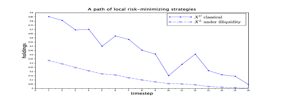
(a) Hedging with only the Future $F^{2}$ which has the same delivery period as the claim $H$. The hedging strategy $X^{C}$ corresponds to the classical case without liquidity cost and $X^{L}$ to the case with constant liquidity structure (105) with parameters $M_{2}=N_{2}=0.01$. Observe that the optimal LRM-strategy $X^{L}$ under illiquidity is less volatile than the classical LRM-strategy $X^{C}$.

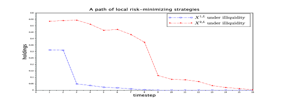
(b) Hedging with the two futures $F^{1}$ and $F^{3}$ with consecutive delivery periods which together cover the delivery period of the claim $H$. Both futures have a time-varying liquidity structure (4.2.1) with parameters $M_{1}=M_{3}=0.005,N_{1}=2M_{1},N_{3}=2M_{3}$. The optimal LRM-strategy $X^{1,L}$ under illiquidity corresponds to the future $F^{1}$ and $X^{2,L}$ to the future $F^{3}$ which is more liquid and expires later than $F^{1}$. $F^{3}$ is used more actively as can be observed from the plot. In the delivery period both futures become very illiquid and thus a rapid drop in the holdings can be observed.

Figure 1: Comparison of the sample path of optimal LRM-strategies under different liquidity structures and for different hedge instruments. All plots based on the same realization of the underlying.

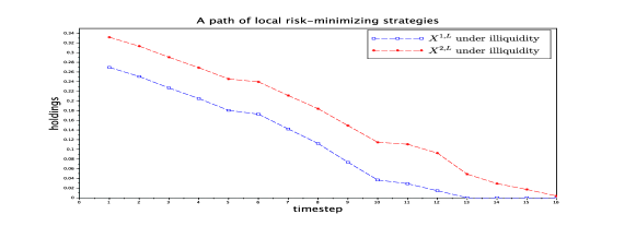
(a) Hedging with the two Futures $G^{1},G^{2}$ with constant liquidity structure (105) with parameters $M_{i}=N_{i}=0.01$ for $i=1,2$ .

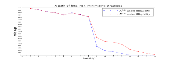
(b) Hedging with two instruments using the Futures $G^{1},G^{2}$ with time-varying liquidity structure (4.2.1) with parameters $M_{i}=0.005,N_{i}=2M_{i}$ for $i=1,2$. The sudden drop in the holdings occurs when entering the delivery period where the futures are very illiquid.

Figure 2: Comparison of the sample path of optimal LRM-strategies under different liquidity structures but with the same hedge instruments. The two futures have overlapping delivery periods starting together but $G^{1}$ expires earlier. The delivery period of $G^{2}$ is the same as the one of the claim $H$. The LRM-strategies $X^{1,L},X^{2,L}$ under illiquidity correspond to the future hedge instruments $G^{1},G^{2}$ respectively.

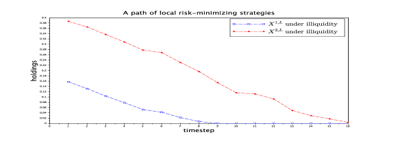
(a) Hedging with the two Futures $G^{2},G^{3}$ with constant liquidity structure (105) with parameters $M_{i}=N_{i}=0.01$ for $i=2,3$.

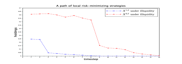
(b) Hedging with the two Futures $G^{2},G^{3}$ with time-varying liquidity structure (4.2.1) with parameters $M_{i}=0.005,N_{i}=2M_{i}$ for $i=2,3$.

Figure 3: Comparison of the sample path of optimal LRM-strategies under different liquidity structures but with the same hedge instruments. The two futures have consecutive delivery periods with the one of $G^{3}$ starting earlier. The delivery period of $G^{2}$ and the claim $H$ coincide. The optimal LRM-strategy $X^{1,L}$ under illiquidity corresponds to the hedge instrument $G^{3}$ and $X^{2,L}$ to $G^{2}$.

5 Conclusion

In an arbitrage-free model framework, this paper has presented a new quadratic hedging criterion that targets at minimizing the risk against random fluctuations of the underlying stock price while simultaneously incurring low liquidity costs. It extends the quadratic local-risk minimization approach of Schweizer (1988) in the spirit of Rogers & Singh (2010) and Agliardi & Gençay (2014). It is mathematically tractable enough to allow for computable formulae. Under mild conditions, the optimization problem can be solved in closed-form. Furthermore, by embedding a multi-dimensional price process with different maturities in our setting it is possible to consider as one possible application the hedging of an Asian-style option in an electricity exchange using a variety of futures. In a simulation study we analyze hedge performance and cost under various pairs of futures with different delivery periods and liquidity levels, allowing us to investigate the tradeoff between hedge performance and liquidity cost.

6 Appendix

Proof of Lemma 2.4.

The arguments follow those in the proof of Lemma 1 in Lamberton et al. (1998).

Let $\varphi=(X,Y)$ be a LRM-strategy under illiquidity and fix some $k\in\{0,1,\dots,T-1\}$. Assuming that $C(\varphi)$ is not a martingale, we can choose a local perturbation $\varphi^{\prime}=(X^{\prime},Y^{\prime})$ of $\varphi$ at time $k$ by defining $X^{\prime}:=X$ and only modifying the cash holding $Y^{\prime}$ at time $k$, by adding the conditional expectation of the incremental cost at time $k$ to $Y$,

$$Y_{k}^{{}^{\prime}}:=\mathbb{E}[C_{T}(\varphi)-C_{k}(\varphi)|\mathcal{F}_{k}]+Y_{k}\,.$$ (118)

This implies that $\mathbb{E}[C_{T}(\varphi^{\prime})-C_{k}(\varphi^{\prime})|\mathcal{F}_{k}]=0$ and $\mathbb{V}ar(C_{T}(\varphi^{\prime})-C_{k}(\varphi^{\prime})|\mathcal{F}_{k})=\mathbb{V}ar(C_{T}(\varphi)-C_{k}(\varphi)|\mathcal{F}_{k})$. Since ${\mathbb{E}}[X^{2}]={\mathbb{V}ar}[X]+({\mathbb{E}}[X])^{2}$ for a random variable $X$, one can conclude that using the strategy $\varphi^{\prime}$ the risk process becomes less, that is,

$$R_{k}(\varphi^{\prime})\leq R_{k}(\varphi)\,.$$ (119)

Since $X^{\prime}:=X$, the liquidity costs of $\varphi^{\prime}$ and $\varphi$ equal. This implies,

$$T_{k}^{\alpha}(\varphi^{\prime})\leq T_{k}^{\alpha}(\varphi)\,.$$ (120)

By the fact that $\varphi$ is a LRM-strategy under illiquidity, we must have equality on $T_{k}^{\alpha}$ which implies equality on $R_{k}$ i.e., $R_{k}(\varphi^{\prime})=R_{k}(\varphi)$. So, the cost process $C(\varphi)$ must be a martingale. ∎

Proof of Lemma 2.5.

As in Lamberton et al. (1998) (see proof of Proposition 2), by using Lemma 2.4 and the fact that

$$\mathbb{E}[C_{T}(\varphi^{\prime})-C_{k}(\varphi^{\prime})|\mathcal{F}_{k}]=\Delta C_{k+1}(\varphi^{\prime}),$$ (121)

which follows from the martingale property of $C(\varphi)$, one can conclude that

$$R_{k}(\varphi^{\prime})=\mathbb{E}[R_{k+1}(\varphi)|\mathcal{F}_{k}]+\mathbb{E}[(\Delta C_{k+1}(\varphi^{\prime}))^{2}|\mathcal{F}_{k}]\,.$$ (122)

Furthermore since $\varphi^{\prime}$ is a local perturbation of $\varphi$ at time $k$, we have

$$\mathbb{E}[(X^{\prime}_{k+2}-X^{\prime}_{k+1})^{*}[S_{k+1}(X^{\prime}_{k+2}-X^{\prime}_{k+1})-S_{k+1}(0)]|\mathcal{F}_{k}]$$

$$\quad=\mathbb{E}[(X_{k+2}-X^{\prime}_{k+1})^{*}[S_{k+1}(X_{k+2}-X^{\prime}_{k+1})-S_{k+1}(0)]|\mathcal{F}_{k}]$$ (123)

and the claim follows. ∎

Proof of Proposition 2.6.

The proof follows the steps in the proof of Proposition 2 in Lamberton et al. (1998).

Let us first show the $``\Leftarrow"$ direction of the proof. We want to show that $\varphi=(X,Y)$ is a LRM-strategy under illiquidity, according to Definition 2.3. So, fix some $k\in\{0,1,\dots,T-1\}$ and let $\varphi^{\prime}=(X^{\prime},Y^{\prime})$ be a local perturbation of $\varphi$ at time $k$.

Since property (i) holds and $\varphi^{\prime}$ a local perturbation of $\varphi$ at time $k$ then by Lemma 2.5 we have the equality

$$T_{k}^{\alpha}(\varphi^{\prime})= \mathbb{E}[R_{k+1}(\varphi)|\mathcal{F}_{k}]+\mathbb{E}[(\Delta C_{k+1}(\varphi^{\prime}))^{2}|\mathcal{F}_{k}]$$

$$+\alpha\mathbb{E}[(X_{k+2}-X^{\prime}_{k+1})^{*}[S_{k+1}(X_{k+2}-X^{\prime}_{k+1})-S_{k+1}(0)]|\mathcal{F}_{k}]$$ (124)

Moreover, from the definition of the conditional variance we have

$$\mathbb{E}[(\Delta C_{k+1}(\varphi^{\prime}))^{2}|\mathcal{F}_{k}]\geq\mathbb{V}ar(\Delta C_{k+1}(\varphi^{\prime})|\mathcal{F}_{k})$$ (125)

and so we can estimate

$$T_{k}^{\alpha}(\varphi^{\prime})\geq\, \mathbb{E}[R_{k+1}(\varphi)|\mathcal{F}_{k}]+\mathbb{V}ar(\Delta C_{k+1}(\varphi^{\prime})|\mathcal{F}_{k})$$

$$+\alpha\mathbb{E}[(X_{k+2}-X^{\prime}_{k+1})^{*}[S_{k+1}(X_{k+2}-X^{\prime}_{k+1})-S_{k+1}(0)]|\mathcal{F}_{k}]\,.$$ (126)

Since $\varphi^{\prime}$ a local perturbation of $\varphi$ at time $k$ then $X^{\prime}_{k+2}=X_{k+2}$ and $Y^{\prime}_{k+1}=Y_{k+1}$ and so we get

$$\mathbb{V}ar(\Delta C_{k+1}(\varphi^{\prime})|\mathcal{F}_{k})=\mathbb{V}ar(C_{k+1}(\varphi^{\prime})|\mathcal{F}_{k}) =\mathbb{V}ar(V_{k+1}(\varphi^{\prime})-(X^{\prime}_{k+1})^{*}\Delta S_{k+1}|\mathcal{F}_{k})$$

$$=\mathbb{V}ar(V_{k+1}(\varphi)-(X^{\prime}_{k+1})^{*}\Delta S_{k+1}|\mathcal{F}_{k})$$ (127)

and we can conclude that

$$T_{k}^{\alpha}(\varphi^{\prime})\geq\, \mathbb{E}[R_{k+1}(\varphi)|\mathcal{F}_{k}]+\mathbb{V}ar(V_{k+1}(\varphi)-(X^{\prime}_{k+1})^{*}\Delta S_{k+1}|\mathcal{F}_{k})$$

$$+\alpha\mathbb{E}[(X_{k+2}-X^{\prime}_{k+1})^{*}[S_{k+1}(X_{k+2}-X^{\prime}_{k+1})-S_{k+1}(0)]|\mathcal{F}_{k}]\,.$$ (128)

Furthermore, since (ii) holds, then

$$T_{k}^{\alpha}(\varphi^{\prime})\geq\, \mathbb{E}[R_{k+1}(\varphi)|\mathcal{F}_{k}]+\mathbb{V}ar(V_{k+1}(\varphi)-(X_{k+1})^{*}\Delta S_{k+1}|\mathcal{F}_{k})$$

$$+\alpha\mathbb{E}[(X_{k+2}-X_{k+1})^{*}[S_{k+1}(X_{k+2}-X_{k+1})-S_{k+1}(0)]|\mathcal{F}_{k}]\,.$$ (129)

On the other hand, we have by definition (see Equation (12) )

$$T_{k}^{\alpha}(\varphi)=R_{k}(\varphi)+\alpha\mathbb{E}[\Delta X_{k+2}^{*}[S_{k+1}(\Delta X_{k+2})-S_{k+1}(0)]|\mathcal{F}_{k}]\,.$$ (130)

Since $C(\varphi)$ is a martingale, we get the representation (14) for the risk process $R_{k}(\varphi)$. So we can conclude that

$$T_{k}^{\alpha}(\varphi)= \mathbb{E}[R_{k+1}(\varphi)|\mathcal{F}_{k}]+\mathbb{V}ar(\Delta C_{k+1}(\varphi)|\mathcal{F}_{k})$$

$$+\alpha\mathbb{E}[(X_{k+2}-X_{k+1})^{*}[S_{k+1}(X_{k+2}-X_{k+1})-S_{k+1}(0)]|\mathcal{F}_{k}]$$ (131)

Finally, since (6) and (6) hold then $T_{k}^{\alpha}(\varphi^{\prime})\geq T_{k}^{\alpha}(\varphi)$ and this shows the $``\Leftarrow"$ direction of the proof.

Now, assuming that $\varphi$ is a LRM-strategy under illiquidity i.e., $T_{k}^{\alpha}(\varphi^{\prime})\geq T_{k}^{\alpha}(\varphi)$ for any local perturbation $\varphi^{\prime}$ of $\varphi$ at time $k$, we will show the $``\Rightarrow"$ direction of the proof. Property (i) holds from Lemma 2.4. So it remains to show Property (ii).

Since $C(\varphi)$ is a martingale and $\varphi^{\prime}$ a local perturbation of $\varphi$ at time $k$, then from Lemma 2.5 we know that equation (2.5) holds. On the other hand, since (6) holds (from the martingale property of $C(\varphi)$) then from the fact that $T_{k}^{\alpha}(\varphi^{\prime})\geq T_{k}^{\alpha}(\varphi)$ we have

$$\mathbb{E}[R_{k+1}(\varphi)|\mathcal{F}_{k}]+\mathbb{E}[(\Delta C_{k+1}(\varphi^{\prime}))^{2}|\mathcal{F}_{k}]$$

$$\quad+\alpha\mathbb{E}[(X_{k+2}-X^{\prime}_{k+1})^{*}[S_{k+1}(X_{k+2}-X^{\prime}_{k+1})-S_{k+1}(0)]|\mathcal{F}_{k}]$$

$$\geq\mathbb{E}[R_{k+1}(\varphi)|\mathcal{F}_{k}]+\mathbb{V}ar(\Delta C_{k+1}(\varphi)|\mathcal{F}_{k})$$

$$\quad+\alpha\mathbb{E}[(X_{k+2}-X_{k+1})^{*}[S_{k+1}(X_{k+2}-X_{k+1})-S_{k+1}(0)]|\mathcal{F}_{k}]$$ (132)

and from the definition of the conditional variance we can conclude that

$$\mathbb{V}ar(\Delta C_{k+1}(\varphi^{\prime})|\mathcal{F}_{k})+(\mathbb{E}[\Delta C_{k+1}(\varphi^{\prime})|\mathcal{F}_{k}])^{2}$$

$$\quad+\alpha\mathbb{E}[(X_{k+2}-X^{\prime}_{k+1})^{*}[S_{k+1}(X_{k+2}-X^{\prime}_{k+1})-S_{k+1}(0)]|\mathcal{F}_{k}]$$

$$\geq\mathbb{V}ar(\Delta C_{k+1}(\varphi)|\mathcal{F}_{k})+\alpha\mathbb{E}[(X_{k+2}-X_{k+1})^{*}[S_{k+1}(X_{k+2}-X_{k+1})-S_{k+1}(0)]|\mathcal{F}_{k}]$$ (133)

for all $X^{\prime}_{k+1}$ and $Y^{\prime}_{k}$. Fixing $X^{\prime}_{k+1}$ and choosing $Y^{\prime}_{k}$ as in the proof of Lemma 2.4 the inequality still holds and the liquidity costs remain unchanged. Since this choice gives us $\mathbb{E}[\Delta C_{k+1}(\varphi^{\prime})|\mathcal{F}_{k}]=0$ (as in the proof of Lemma 2.4) and since $\varphi^{\prime}$ a local perturbation of $\varphi$ at time $k$, we get the inequality

$$\mathbb{V}ar(V_{k+1}(\varphi)-(X^{\prime}_{k+1})^{*}\Delta S_{k+1}|\mathcal{F}_{k})$$

$$\quad\quad+\alpha\mathbb{E}[(X_{k+2}-X^{\prime}_{k+1})^{*}[S_{k+1}(X_{k+2}-X^{\prime}_{k+1})-S_{k+1}(0)]|\mathcal{F}_{k}]$$

$$\geq \mathbb{V}ar(V_{k+1}(\varphi)-(X_{k+1})^{*}\Delta S_{k+1}|\mathcal{F}_{k})$$

$$\quad\quad+\alpha\mathbb{E}[(X_{k+2}-X_{k+1})^{*}[S_{k+1}(X_{k+2}-X_{k+1})-S_{k+1}(0)]|\mathcal{F}_{k}]\,.$$ (134)

This shows that Property (ii) holds and the proof is completed. ∎

References

- Agliardi & Gençay (2014) Agliardi, R. & Gençay, R. (2014). Hedging through a limit order book with varying liquidity. Journal of Derivatives, 22(2), 32–49.
- Bank & Baum (2004) Bank, P. & Baum, D. (2004). Hedging and portfolio optimization in financial markets with a large trader. Mathematical Finance, 14(1), 1–18.
- Bank et al. (2017) Bank, P., Soner, H., & Voß, M. (2017). Hegding with temporary price impact. Math. Finan. Econ., 11, 215–239.
- Benth & Detering (2015) Benth, F. & Detering, N. (2015). Pricing and Hedging Asian-style options on energy. Finance & Stochastics, 19(4), 849–889.
- Benth et al. (2015) Benth, F., Lange, N., & Myklebust, T. (2015). Pricing and Hedging Quanto Options in Energy Markets. Journal of Energy Markets, 8(1), 1– 35.
- Benth et al. (2007) Benth, F., Meyer-Brandis, T., & Kallsen, J. (2007). A non-Gaussian Ornstein-Uhlenbeck process for electricity spot price modeling and derivatives pricing. Appl. Math. Fin., 14(2), 153–169.
- Beutner (2007) Beutner, E. (2007). Mean–variance hedging under transaction costs. Mathematical Methods of Operations Research, 65(3), 539–557.
- Çetin et al. (2004) Çetin, U., Jarrow, R., & Protter, P. (2004). Liquidity risk and arbitrage pricing theory. Finance and Stochastics, 8.
- Çetin et al. (2010) Çetin, U., Soner, H., & Touzi, N. (2010). Option hedging for small investors under liquidity costs. Finance and Stochastics, 14(3), 317–341.
- Coleman et al. (2003) Coleman, T., Li, Y., & Patron, M. (2003). Discrete hedging under piecewise linear risk minimization. Journal of Risk, 5(3), 39–65.
- Föllmer & Sondermann (1986) Föllmer, H. & Sondermann, D. (1986). Hedging of non-redundant contingent claims. In W. Hildenbrand, A. M.-C. E. (Ed.), Contributions to Mathematical Economics, (pp. 205–223). North-Holland.
- Fries (2007) Fries, C. (2007). Mathematical Finance: Theory, Modeling, Implementation. Wiley.
- Gökay et al. (2011) Gökay, S., Roch, A., & Soner, H. (2011). Liquidity models in continuous and discrete time. In G., D. N. & B., Ø. (Eds.), Advanced Mathematical Methods for Finance, (pp. 333–365). Springer.
- Gökay & Soner (2012) Gökay, S. & Soner, H. (2012). Liquidity in a binomial market. Mathematical Finance, 22(2), 250–276.
- Horn & Johnson (2012) Horn, R. & Johnson, C. (2012). Matrix Analysis. Cambridge University Press.
- Lamberton et al. (1998) Lamberton, D., Pham, H., & Schweizer, M. (1998). Local risk-minimization under transaction costs. Mathematics of Operations Research, 23, 585–612.
- Løkka (2012) Løkka, A. (2012). Optimal execution in a multiplicative limit order book. Preprint, London School of Economics.
- Longstaff & Schwartz (2001) Longstaff, F. & Schwartz, E. (2001). Valuing American options by simulation: A simple least-squares approach. Review of Financial Studies, 14(1), 113–147.
- Motoczyński (2000) Motoczyński, M. (2000). Multidimensional variance-optimal hedging in discrete-time model—a general approach. Mathematical Finance, 10(2), 243–257.
- Roch (2011) Roch, A. (2011). Liquidity risk, price impacts and the replication problem. Finance and Stochastics, 15, 399.
- Rogers & Singh (2010) Rogers, L. & Singh, S. (2010). The cost of illiquidity and its effects on hedging. Mathematical Finance, 20(4), 597–615.
- Schäl (1994) Schäl, M. (1994). On quadratic cost criteria for option hedging. Mathematics of Operations Research, 19(1), 121–131.
- Schweizer (1988) Schweizer, M. (1988). Hedging of options in a general semimartingale model. Dissertation, ETH Zurich, 8615.
- Schweizer (1995) Schweizer, M. (1995). Variance-optimal hedging in discrete time. Mathematics of Operations Research, 20, 1–32.
- Schweizer (2001) Schweizer, M. (2001). A guided tour through quadratic hedging approaches. In Cvitanic, J., Jouini, E., & (Eds.), M. M. (Eds.), Option Pricing, Interest Rates and Risk Management, (pp. 538–574). Cambridge University Press.