*

Abstract. This thesis presents original results in two domains of disordered statistical physics: logarithmic correlated Random Energy Models (logREMs), and localization transitions in long-range random matrices.

In the first part devoted to logREMs, we show how to characterise their common properties and model–specific data. Then we develop their replica symmetry breaking treatment, which leads to the freezing scenario of their free energy distribution and the general description of their minima process, in terms of decorated Poisson point process. We also report a series of new applications of the Jack polynomials in the exact predictions of some observables in the circular model and its variants. Finally, we present the recent progress on the exact connection between logREMs and the Liouville conformal field theory.

The goal of the second part is to introduce and study a new class of banded random matrices, the broadly distributed class, which is characterid an effective sparseness. We will first study a specific model of the class, the Beta Banded random matrices, inspired by an exact mapping to a recently studied statistical model of long–range first–passage percolation/epidemics dynamics. Using analytical arguments based on the mapping and numerics, we show the existence of localization transitions with mobility edges in the “stretch–exponential” parameter–regime of the statistical models. Then, using a block–diagonalization renormalization approach, we argue that such localization transitions occur generically in the broadly distributed class.

Remerciements

I am grateful to Jonathan Keating and Christopher Mudry who kindly accepted to be the Referees of the thesis manuscript.

It is a pleasure to acknowledge Yan Fyodorov as a senior collaborator. His pioneering scientific works have been inspiring the original research reported in both parts of this thesis. Although we have only met once physically, I have learned a lot from him through our collaboration. Besides playing key rôles in our joint works (published and ongoing), he has been a careful reader of our other works, and shared his insights and suggestions.

Je remercie Bertrand Georgeot et Didina Serban d’avoir accepté d’être Membre du Jury de ma thèse.

Je suis reconnaissant envers M. Gilles Montambaux, qui a suivi mon doctorat en tant que responsable de l’École Doctorale de Physique en Île–de–France. Son attention particulière et ses soutiens constants sont essentiels pour les résultats de mon parcours. J’ai apprécié particulièrement son écoute lors de nos entretiens annuels.

Les travaux qui consituent cette thèse sont les fruits de mes séjours de 2015 à 2017 au sein du Laboratoire de Physique Théorique et Modèles Statistiques (LPTMS), qui m’a soutenu à tous les moments décisifs, et qui m’a accueilli dans son ambience vivante et travailleuse, indispensable pour mon emancipation scientifique. Je remercie tout particulièrement son directeur Emmanuel Trizac pour sa confiance et ses encouragements, sans lesquels j’aurais abandonné la recherche depuis longtemps. Mes gratitudes les plus spéciales vont à Claudine Le Vaou, la gestionnaire du laboratoire. C’est grâce à ses compétences et créativités exceptionnelles, et à son attention et bienveillence sans faille, que nous avons résoulu les nombreux problèmes administratifs hautement non–triviaux, qui sont les conditions sine qua non du bon déroulement de ma thèse. Je remercie également Barbara Morléo, collègue de Claudine au CNRS, pour ses efforts aussi importants sur mon dossier. Je remercie les informaticiens du laboratoire, Vincent Degat et Qin Zhiqiang: tous les deux ont sauvé ma vie en sauvant mes données. D’ailleurs, le puissant cluster du LPTMS est derrière toutes les études numériques de cette thèse. Enfin, un merci spécial va à Marie–Thérèse Commault pour sa gentillesse.

Au LPTMS, j’ai eu l’occastion de discuter régulièrement avec plusieurs membre permanents. M’excusant d’être non–exlusif, je remercie particulièrement: Eugène Bogomolny pour ses nombreux conseils pointus, Silvio Franz pour m’avoir appris la théorie des verres de spin, et Christophe Texier, pour ses explications lucides sur des sujets difficiles comme la localisation d’Anderson; outre la recherche, les suggestions de Martin Lenz et Satya Majumdar ont été extrêmement utiles pour ma recherche de post–doc. Je suis heureux d’avoir connu mes camarades du bureau, et surtout mes co–disciples, Clélia de Mulatier, Inès Rodriguez Arias, et (de façon non-officielle) Timothée Thiery; je remercie tous les trois pour leur encouragement et sympathie. J’ai apprécié les discussions avec le brilliant et aimable post–doc Andrea De Luca.

Mes travaux ont également été soutenus par Capital Fund Management. Je remercie la générosité du groupe, et tout particulièrement son président Jean–Philippe Bouchaud, sans qui cela aurait été impossible. Je voudrais remercier une autre fois Jean–Philippe, en tant que physicien, parce que j’ai eu la chance de participer à la collaboration scientifique qu’il avait initiée, et qui est à l’origine des résultats du Chapitre 3 de cette thèse. Ses idées et ses grandes qualités intellectuelles m’ont toujours inspiré. Mon seul regret, auquel je compte remédier dans un futur proche, est de ne pas avoir suffisamment travaillé sur notre projet commun pendant la thèse.

Je remercie Pierre Le Doussal d’avoir été un mentor et collaborateur important, bien qu’il ne soit pas mon directeur de thèse officiel. Il a porté son attention encourageante à mon travail avant le début de nos collaborations. En particulier, grâce à son soutien, j’ai fait mon premier voyage de recherche, à Santa–Barbara, pendant trois semaines riches et fructueuses. À risque de reprendre les mots de ses anciens élèves, les entretiens réguliers avec Pierre sont des moments précieux, qui font disparaitre toutes les angoisses du quotidien, grâce à l’enthousiasme scientifique infini de Pierre. De cela s’ensuivent son attention acharnée aux détails et son jusqu’au–boutism (dans le sens strictement positif du terme!) qui ne cesseront d’être mes références.

Avant d’arriver au LPTMS, j’ai été étudiant à l’Institut de Physique Théorique (IPhT) à Saclay, sous la direction de Kirone Mallick, que je tiens à remercier. C’est Kirone, et Bernard Derrida, notre professeur de Master 2, qui m’avaient initié à la recherche en physique statistique. Au–delà du savoir–faire scientifique, Kirone m’a offert les leçons les plus précieuses que puisse recevoir un chercheur débutant: l’humilité, la préserverence, et l’ouverture d’esprit. Il a toujours été encourageant et de bons conseils, même quand j’avais l’intention de changer de sujet et de laboratoire. Cette transition n’aurait pas été possible sans sa bienveillence altruiste. Je remercie également Stéphane Nonnenmacher et Michel Bauer, directeurs de l’IPhT, d’avoir facilité ce transfert. Parmi les membres de l’IPhT, je voudrais remercier particulièrement: Jérémie Bouttier, pour les discussions scientifiques, et surtout pour m’avoir fait venir à Cargèse; Sylvain Ribault, pour les discussions, et pour ses codes open–source et ses notes de cours en domaine public sans lesquels une partie importante de cette thèse serait absente.

Enfin, je ne remercierai jamais assez Alberto et Raoul, mes directeurs de thèse au LPTMS (d’ailleurs, Raoul a dirigé mon stage M2). La longueur de ce texte divergerait si je me mettais à énumerer leurs générosités, sans lesquelles la longueur du texte qui suit serait proche de zéro. Je leur dédie donc ce manuscrit comme je le fais à ma famille.

致父母与爱妻佳骊。

The bibliography style of this thesis is provided by SciPost, an open–access online journal of Physics.

Foreword

With the invention of the microscope, a new world was discovered. It was considered so radically different from the macroscopic world that, according to Michel Foucault’s account , it led to the modern concept of life. It was in terms of the latter that the irregular motion of pollens observed by Brown was understood, until Einstein (theory, 1905) and Perrin (experiment, 1908) put on a firm footing the idea that all natural phenomena, beyond the realm of life, and as simple as the expansion of heated gas, have a microscopic origin. Unfortunately, that was too late to change the tragic life of the idea’s father, Boltzmann, on whose tombstone was graved the following equation

$$S=k\log W$$

relating the macroscopic quantity, entropy ($S$) to a microscopic one, the number of microscopic configurations ($W$). The Boltzmann constant $k$ is as fundamental as the Planck’s constant $\hbar$: its numerical value is only a consequence of choice of units. In this thesis, we use units so that $k=\hbar=1$.

With this equation was born the subject of statistical physics, i.e., the physics of counting large numbers ($W$ in the above equation). With quantum mechanics, it is one of the pillars of modern condensed matter theory. The standard paradigm of the latter was summarized by the Anderson’s beautiful formula more is different [2] in 1972. When a large number of microscopic constituents organize themselves, some symmetry of the constituent law can be spontaneously broken, leading to phase transitions. About the same time, it was realized that spontaneous symmetry breaking and phase transitions can be described theoretically by quantum/statistical field theory and the renormalization group. The latter led to, in principle, a classification of the states of matter in terms of universality classes. Each of the latter is characterised by a small set of “critical exponents”, which are independent of the microscopic nature of the constituents. The classification was carried out most successfully in two (or $1+1$) dimensions, thanks to the powers of conformal field theory (CFT).

However, the success is largely limited to systems that reach rapidly enough their thermal equilibrium. Extending the paradigm to phenomena far from equilibrium (such as turbulence) is a largely open challenge. In this respect, a crucial intermediate is the disordered systems: glasses, electronic systems with impurities, etc. They are not strongly driven (like turbulent fluids) or active (like many biological systems), so the equilibrium formalism is still applicable. However, the existence of a large hierarchy of time–scales brings an essential complication: the quenched randomness in the microscopic Hamiltonian. As a consequence, the equilibration is only partial, and the system may visit a fraction of the complex energy landscape. This led to new notions of phase transition and symmetry breaking, such as localization transition and replica symmetry breaking (RSB). Their field theory description is not always known (e.g., the plateau transition in the integer quantum Hall effect), and the known ones have limited range of applications, and involve often technicalities such as super–symmetry (localization transitions) and/or functional renormalization group (manifolds in random media).

In this respect, the statistical physics theory of disordered systems is largely driven by specific models, i.e., their analytic solutions and relations/mappings between them. The goal is to identify new universality classes, clarify the universal and non–universal properties of the particular models, and seek their field theory description. This is the method of the present thesis. It has two subjects: logarithmically correlated Random Energy Model (logREM) (Chapter 2) and localization transition with long–range hopping (Chapter 3). Although they are largely independent, their study shares a few common notions and methods, such as extreme value statistics and theoretical models known as polymers in random media. The purpose of Chapter 1 is to introduce these basic notions, whereas Chapter 4 summarizes the thesis and discusses the perspective from a global point of view.

LogREM
Overview of Chapter 2

LogREM are arguably the simplest, yet non–trivial, class of disordered statistical models. They can be defined as the problem of a thermal particle in a random potential. Since Sinai’s study of the case where the random potential is a 1d Brownian motion, such problems have become prototypes of statistical physics with disorder. The logREM correspond to cases where the potential is Gaussian and logarithmically correlated. From a theoretical point of view (reviewed in section 1.2), this is arguably the most interesting case, because as the result of competition between deep valleys of the potential and the entropic spreading of the particle, there is a freezing transition at some finite temperature. The low–temperature, “frozen”, phase is extremely glassy, in the sense that the thermal particle is caged in a few deepest valleys of the potential. Remarkably, logREM are among the few cases where the method of RSB is applicable in finite dimensional problems. The essential reason is that, the class of logREM contains not only the problem of a thermal particle in log–correlated potentials, but also that of directed polymers on the Cayley tree (DPCT), and of Branching Brwonian motion (BBM). These are all mean–field statistical models defined on hierarchical (tree–like) lattices, where the RSB is known to apply.

This fundamental link between finite–dimensional and hierarchical models has an involved history going back to the Random Energy Model (REM) of spin glass, of which logREM are close cousins. The main driving force behind the discovery of the link are the study of 2D disordered systems: Dirac fermions in random magnetic field, and random–gauge XY model. The randomness behind these models reduces all to the 2D Gaussian Free Field (GFF), which is one of the most natural ways to construct log–correlated potentials. They lead either to 2D logREM, or to 1D logREM, by restricting the thermal particle to a 1D geometry in the plane where the 2D GFF is defined. To be fair, it must be mentioned that another way of generating 1D log–correlated potential comes from random matrices (through the logarithm of their characteristic polynomial) and number theory (Riemann $\zeta$ function on the critical line): this unexpected link to pure mathematics has stimulated many recent developments.

Therefore, the domain of logREM has become a inter–disciplinary area attracting the attention of theoretical physicists and mathematicians alike. In this respect, the point of view and the original contributions of this thesis are focused on the 2D GFF–related aspects. Indeed, many questions that we will investigate can be asked on a single logREM, the circular model, and its variants. Put simply, it describes a thermal particle confined onto the unit circle, on which a random potential is defined by restricting a 2D GFF to the circle (from the random matrix point of view, one would define as the log of the characteristic polynomial of a random unitary matrix). Now, we may ask:

• Why, historically speaking, do theorists come to study this model? What is already known about it (section 2.1 except 2.1.4)?

• What is the relation between the above continuum definition and its discrete definitions (section 2.2.2)?

• What is the thermodynamics of the model, why does it have a freezing transition? Why and how can we study it using RSB ? What are the general consequences of this approach to logREM (sections 2.2.1 and 2.3)?

• What is full distribution of the free energy (this is known and reviewed in section 2.1.3)? How does it depend on the specific definition of the model? What if we consider a realistic 2D GFF on a finite domain, such as a disk with Dirichlet boundary condition (section 2.4.2)?

• What other observables can we calculate for the circular model? Are there some analytical tools that can be systematically applied (a candidate is the Jack polynomials, see section 2.4)?

• In the low temperature phase, the thermal particle is caged in a few deepest minima of the potential. How do they behave, i.e., what is the extreme order statistics? How can we study them using the RSB approach? For instance, how can we predict the distribution of gap between the deepest and second minimal values (section 2.5)?

As we will see, the sections 2.1, 2.2, 2.3 and 2.5 are based on results which apply to general logREM, but we discuss them using the same example of circular model for the sake of concreteness. On the other hand, most of the results of section 2.4 are specific to the circular model and its variants.

Therefore, using the circular model, we have provided an overview of Chapter 2, excluding section 2.6 on the relation between Liouville field theory (LFT) and logREM, and the sections 2.1.4, 2.2.3 and 2.3.4, whose essential purpose is to provide conceptional preparations for the relation. Relating precisely LFT and logREM is one of the main contributions of this manuscript. Although it does rely on some of the general results obtained in the previous sections (in particular, those in section 2.5 concerning the full minima process), section 2.6 is quite detached from the rest of the Chapter: for example, we will start from a genuinely 2D logREM (while the circular model is defined on a 1D geometry); also, we will be focused on the Gibbs measure (the position of thermal particles) instead of the free energy and minimal values. Therefore, we refer to section 2.6.1 for a more specific overview. The original results of section 2.6 are recent; they are impacting considerably how we view logREM in general, and raised many new questions that are under active investigation. These questions, as well as those raised by the previous sections, are discussed informally in section 2.7.

Localization transition with long–range hopping
Overview of Chapter 3

Localization transitions are arguably the most prototypical and most fascinating phenomena usually associated to disordered systems. With regard to the previous Chapter on logREM, freezing transition could also be viewed as a localization transition, in which the classical, thermal particle is caged in few sites. However, properly speaking, the term “localization transitions” is reserved to the quantum mechanics of particles in random potentials. At a formal level, this implies that the fundamental random object is not the partition function or the Gibbs measure, but the Hamiltonian, i.e., a random matrix and its eigenvectors (eigenstates). The latter can be localized or extended (with respect to the basis usually corresponding to the positions of the quantum particle). The sharp changes between the two possibilities (i.e., localization transitions), and the existence of other intermediate ones, are non–trivial questions with important physical applications .

Given the importance of localization transitions, there are many theoretical techniques to study them. The one mainly employed by Chapter 3 is classic and based on the following well–known lesson of Feynman: one can turn a quantum mechanics problem of a particle into a classical statistical mechanics problem of a 1D extended object. In this thesis, this 1D object will be called a polymer. Indeed, it is known that random matrices and their eigenvector localization can be studied by mapping to the problem of polymers in random media. In turn, the latter models found themselves in a well–known web of mappings, which relate them to models of first–passage percolation (FPP) and out–of–equilibrium growth. We will review these relations in section 1.3. The starting point of the original material in Chapter 3 is to extend this web of mappings to the context involving long–range hopping.

The out–come of the new mappings is that, starting from the recently studied long–range FPP/growth models (reviewed in section 3.2), we defined a new ensemble of random matrices, the Beta Banded Random Matrices (BBRM). They turn out to be superficially comparable to the Power-law Banded Random Matrices (PBRM). As we will review in 3.1, the PBRM were studied as 1D, long–range proxies of the standard Anderson model, which has no localization transition in 1D and 2D; however, the localization transition of the PBRM is pathologically simple and has in particular no mobility edges (i.e., separation of the spectrum of one matrix into localized and extended eigenstates). Remarkably, as we will explore in section 3.3, the new BBRM turn out to have a different and richer phase diagram from PBRM, and have in particular localizations transitions with mobility edges. To show this, we will use the mapping that motivated the model (section 3.3.3), along with other arguments and numerical evidences, in section 3.3.4.

Nonetheless, we would like to emphasize that the main interest of Chapter 3 is not the results on the specific BBRM model, but their generalization to a larger class of banded random matrices with broadly distributed elements, in section 3.4. Roughly speaking, such matrices are sparse: the moments of the matrix elements are much larger than their typical values, so most of the elements are small, but there are a few “black swans”. This turns out to be the most important feature of the BBRM model, and the one that is behind many of its localization properties. The essential point of our demonstration is that, although the exact mapping to the long–range FPP/growth models is limited to the BBRM, the methods used to study the statistical models can be adapted to the “quantum” (random matrix) context, with much looser constraints on the matrices’ properties. Therefore, we shall conclude 3 by predicting the existence of localization transitions for a large class of new banded random matrices. This raises many open questions, which we will discuss in section 3.5.

Publication List

The original research results on which this thesis is based are also available in the following peer-reviewed publications or preprints under review:

• [3] cao15gff.
  Reported in: sections 2.4.1 and 2.4.2.

• [4] cao16maxmin.
  Reported in: sections 2.4.4 and 2.4.3.

• [5] cao16loc.
  Reported in: sections 3.3 and 3.4.

• [6] cao16order.
  Reported in: sections 2.2.1, 2.2.2, 2.4.3, 2.3, and 2.5.

• [7] cao16liouville.
  Reported in: section 2.6.

Acronyms

1RSB

one–step replica symmetry breaking

BBM

Branching Brwonian motion

BBRM

Beta Banded Random Matrix

CFT

conformal field theory

DoS

density of states

DOZZ

Dorn-Otto and Zamolodchikov-Zamolodchikov

DPCT

directed polymers on the Cayley tree

FPP

first–passage percolation

GFF

Gaussian Free Field

i.i.d.

independent and identically distributed

IPR

inverse participation ratio

IR

infra–red

KPP

Kolmogorov–Petrovsky–Piscounov

KPZ

Kardar–Parisi–Zhang

LFT

Liouville field theory

logREM

logarithmically correlated Random Energy Model

OPE

Operator Product Expansion

PBRM

Power-law Banded Random Matrix

pdf

probability density function

PPP

Poisson point process

REM

Random Energy Model

RSB

replica symmetry breaking

SDPPP

randomly shifted, decorated Poisson point process

UV

ultra–violet

Chapter 1 Motivation and overview

1.1 Extreme value statistics

The statistical properties of extreme values among a large number of random variables are relevant in a wide range of disciplines, e.g., statistics, physics, meteorology, and finance. For instance, the knowledge of minimal and maximal stock prices over a period is obviously valuable in financial markets; estimating the most catastrophic flooding that would occur in 100 years is a crucial issue for big cities near water. The distribution of extreme eigenvalues is an important topic in random matrix theory, to which we will come back in Section 1.3.

The basic question of extreme value statistics can be stated roughly as follows: let $V_{1},\dots,V_{M}\in\mathbb{R}$ be $M$ random real variables, what is the distribution of

$$V_{\min}=\min_{i=1}^{M}V_{i}\,,$$ (1.1)

in the limit when $M$ is very large? More precisely speaking, as $M\to\infty$, one seeks to know, in increasing precision: how does the typical value $V_{\min}$ behave, as a function of $M$ ? how much does $V_{\min}$ fluctuate around its typical value? Finally, what is the probability distribution of the fluctuation in the $M\to\infty$ limit? This series of questions leads to the following Ansatz

$$V_{\min}\longrightarrow a_{M}+b_{M}y\,,\,M\to\infty\,.$$ (1.2)

Here the convergence is in distribution. $a_{M}$ the typical value, and $b_{M}$ the amplitude of the fluctuation, are both deterministic numbers that depend on $M$, whereas $y$ is a random variable whose distribution becomes $M$-independent in the $M\to\infty$ limit. The random variable $y=(V_{\min}-a_{M})/b_{M}$ is also called the rescaled minimum. The Ansatz (1.2) is natural, widely applicable, and will apply to all the situations considered in this work. Therefore, in this framework, the problem of extreme value statistics reduces to determining $a_{M}$, $b_{M}$ and the probability distribution of $y$.

Figure 1.1: An illustration of the extreme value statistics problem, and the Ansatz eq. (1.2).

Clearly, the answer depends on the statistical properties of the variables $V_{1},\dots,V_{M}$ themselves, in particular, whether and how they are correlated. A whole chapter of this thesis (Chapter 2) will be devoted to the case where $V_{i}$’s are logarithmically correlated.

Here, let us consider the simplest case where $V_{i}$ are independent and identically distributed (i.i.d.). According to the classical Fisher–Tippett–Gnedenko theorem, the distribution of $y$ belongs to either the Fréchet, Weibull, or the Gumbel family, depending on the asymptotic behaviour of $V_{i}$’s distribution at the $V_{i}\to-\infty$ limit (left tail):

1. When $V_{i}$ has an algebraic left tail, $y$ belongs to the Fréchet family;

2. When $V_{i}$ is bounded from below, $y$ belongs to the Weibull family;

3. Otherwise, $y$ has the Gumbel distribution.

Let us further specialize to an (important) example of the Gumbel case, in which $V_{i}$’s are independent and identically distributed (i.i.d.). Gaussian variables defined by the following mean and covariance

$$\overline{V_{i}}=0\,,\,\overline{V_{i}V_{j}}=2\ln M\delta_{ij}\,,\,i,j=1,\dots,M\,.$$ (1.3)

Then, $V_{\min}$ satisfies the Ansatz eq. (1.2) with the following parameters:

$$a_{M}=-2\ln M+\frac{1}{2}\ln\ln M+\frac{1}{2}\ln(4\pi)\,,\,b_{M}=1\,,\,$$ (1.4a)

$$\mathrm{pdf}(y)=\exp\left(y-e^{y}\right)\stackrel{{\scriptstyle y\to-\infty}}{{\sim}}e^{y}\,,$$ (1.4b)

where $\mathrm{pdf}(y)$ denotes the probability density function (pdf). A self-contained demonstration of this result will be given in section 2.1.1. The strategy will be that of disordered statistical physics:

1. Regard the extreme value $V_{\min}$ as the ground state of a statistical physics model whose energies are $V_{1},\dots,V_{M}$. This means introducing a temperature $T=1/\beta$, and writing down the canonical partition function and the free energy:

   $$\mathcal{Z}=\sum_{i=1}^{M}\exp(-\beta V_{i})\,,\,\mathcal{F}=-\beta^{-1}\ln\mathcal{Z}\,.$$ (1.5)

2. Study the disordered statistical physics model at finite temperature. In particular, determine the limit distribution of the free energy $\mathcal{F}$, in the sense of the scaling Ansatz 1.2. In the statistical physics context, the $M\to\infty$ is usually called the thermodynamic limit. This is the hard core of the approach, since the model defined by eq. (1.5) is disordered, and disordered statistical physics is in general difficult, both analytically and numerically. In the case of the example (1.3), the resulting statistical model is the Derrida’s famous Random Energy Model (REM) [8]. It is one of the foundational toy model in disordered statistical physics; section 2.1.1 will be devoted to it. Its importance can be illustrated by the remarkable fact that such a simple model has a phase transition, at $\beta=\beta_{c}=1$ using the above definition.

3. Take the zero temperature limit, in which $\mathcal{F}$ will tend to $V_{\min}$:

   $$V_{\min}=\lim_{\beta\to+\infty}\mathcal{F}\,.$$ (1.6)

   There is two technical assumptions behind the above statement. First, the absence of zero-temperature phase transition, which assures that the $M\to\infty$ and $\beta\to\infty$ limits commute. Second, the ground should not be degenerated; in particular, the entropy should vanish as $T\to 0$. In the problems treated in this thesis, both assumptions turn out to be fulfilled.

The above relation between extreme value statistics and disordered statistical physics is of central importance and has far more applications. We mention two notable ones. The first is the study of disordered systems (e.g., spin glasses) in low temperatures. Extending the above reasoning, it is natural to expect that this problem is related to the statistical properties of the ground state, and the lowest excited states, which are the higher extreme order statistics of the energies $V_{i}$,

$$V_{\min}=V_{\min,0}\leq V_{\min,1}\leq V_{\min,2}\leq\dots\,,$$ (1.7)

noting that $V_{\min,k}$ is the $(k+1)$-th ordered minimal value. Even when $V_{i}$’s are independent, $V_{\min,k}$’s will be non-trivially correlated, and it is important to characterize the joint distribution of the extrema process. For the Random Energy Model, defined by eq. (1.3), in the $M\to\infty$ limit, the extrema process is known to be the Gumbel Poisson point process. We will discuss this in section 2.5.1.

The second is the statistical physics of optimization problems [9, 10]. Formally, an optimization problem amounts to finding the minimum value and position of some cost function of a (usually large) number of variables, $V(x_{1},\dots,x_{n})$. It is very fruitful to think of the latter as a $n$-dimensional potential energy landscape in a $(n+1)$-dimension space, and the searched minimum is the deepest valley. Many optimization algorithms can be seen as the simulation of a thermal particle in that potential. To understand the behaviour and efficiency of these algorithms, it is the statistical physics of a thermal particle in such a potential.

The notion of potential energy landscape is central in disordered statistical physics and its wide applications. The landscapes involved are often complex, and involve a large of number of parameters unknown a priori. Therefore, their theoretical model is often random potential energy landscapes.

1.2 A thermal particle in a random potential

Random potential energy landscapes studied in spin glass and optimization problems are often in high dimensions. In contrast, the problem of thermal particles in a low-dimensional random potential is easier to state, has its own applications, and remains highly non-trivial.

As an instructive illustration, let us consider Gaussian potentials on a one-dimensional lattice, labelled by $j=0,\dots,M-1$, with periodic boundary condition. Assuming translation invariance, the potential can be generated by Fourier transform

$$V_{j}=\Re\sum_{k=-M/2}^{M/2-1}\sqrt{\mu_{k}}\exp\left(2\pi\mathbf{i}\frac{jk}{M}\right)\mathsf{N}_{k}\,.$$ (1.8)

Here, $(\mathsf{N}_{k})$ is a sequence of i.i.d. standard complex Gaussian variables, and $\mu_{k}\geq 0$ control all the statistical properties of the potential, e.g., the variance and the correlations:

$$\overline{V_{j}^{2}} =\sum_{k=-M/2}^{M/2-1}\mu_{k}\,,\,\overline{V_{0}V_{j}}=\sum_{k=-M/2}^{M/2-1}\mu_{k}\cos\left(\pi\frac{jk}{M}\right)\,,\,$$

$$\overline{(V_{0}-V_{j})^{2}} =\sum_{k=-M/2}^{M/2-1}4\mu_{k}\sin^{2}\left(\pi\frac{jk}{M}\right)\,,$$ (1.9)

The last equation measures the roughness of the potential, and is not affected by the zero-mode $\mu_{k=0}$. Its effect is a trivial global shift to the potential, and will be set to $0$.

Figure 1.2: Samples of random potentials defined by eq. (1.8) and (1.10), with $\alpha=0$ (white noise, left panel) and $\alpha=2$ (Brownian motion, right panel). In the former case, a thermal particle visits freely the whole system, while in the latter, it is confined in the deepest minimum.

An important class of potentials is given by amplitudes $\mu_{k}$ that depend algebraically on $\left|k\right|$; more precisely,

$$\mu_{0}=0\,,\,\mu_{k\neq 0}=\pi M^{-1}\sin^{-\alpha}\left(\frac{\pi\left|k\right|}{M}\right)\stackrel{{\scriptstyle\left|k\right|\ll M}}{{\sim}}k^{-\alpha}M^{\alpha-1}\,.$$ (1.10)

where $\alpha$ is a real parameter. Let us recall the morphology of the potential as function of $\alpha$:

• When $\alpha=0$, $V_{j}$ are i.i.d. standard Gaussian, with variance $\overline{V_{j}^{2}}=1$ (notice the difference with eq. (1.3)). So the potential is a white noise.

• When $\alpha\in(0,1)$, the variance tends to finite constant in the $M\to\infty$ limit, $\overline{V_{j}^{2}}\to\frac{\Gamma\left(\frac{1}{2}-\frac{\alpha}{2}\right)}{\sqrt{\pi}\Gamma\left(1-\frac{\alpha}{2}\right)}$. Off-diagonal correlations decay algebraically: when $1\ll j\ll M$, by eq. (1.9) and (1.10),

  $$\overline{V_{0}V_{j}}\sim\sum_{k}k^{-\alpha}M^{\alpha-1}\cos(\pi jk/M)\sim\left|j\right|^{\alpha-1}\,,$$ (1.11)

  therefore, as $j,M\to\infty$, $\overline{(V_{0}-V_{j})^{2}}$ remains bounded, i.e., the potential is not rough.

• When $\alpha>1$, the potential is rough:

  $$\overline{V_{j}^{2}}\sim M^{2H}\,,\,\overline{(V_{0}-V_{j})^{2}}\sim\left|j\right|^{2H}\,,\,1\ll\left|j\right|\ll M\,,\,H=\frac{\alpha-1}{2}\,,$$ (1.12)

  where $H$ is the Hurst exponent of the roughness. In particular, when $\alpha=2$, the potential can be compared locally to a Brownian motion in a suitable continuum limit, while general $\alpha\in(0,1)$ corresponds to a fractional Brownian motion.

Now, what is the behaviour of a thermal particle of temperature $T=1/\beta$ in one of the above potentials? Note that the statistical model would be formally identical to eq. (1.5), yet with $V_{j}$ non-trivially correlated. A standard strategy of qualitatively understanding any such model is to compare the minimum energy, $V_{\min}=\min_{i=0}^{M-1}(V_{i})$, with the entropy of visiting every one of the $M$ sites $S=\ln M$. This determines roughly whether the system is in an energy-dominating, or entropy-dominating, phase. Such an analysis was carried out in detail in [11], section II, whose main message is the following:

• When $\alpha<1$, $\left|V_{\min}\right|\ll\ln M$. The model has only a high-$T$ phase;

• When $\alpha>1$, $\left|V_{\min}\right|\sim M^{\alpha-1}\gg\ln M$. The model has only a low-$T$ phase. Nevertheless, we note the problem of a thermal particle in a random potential generated by a (fractional) Brownian motion is classic (dating back to Sinai [12]) and well–studied problem with wide applications, see [13] for a review.

Figure 1.3: A sample of the log-correlated random potential, generated by eq. (1.8) and (1.10), with $\alpha=1$. The potential is plotted in the left panel; all its energy values are plotted at the right panel. A thermal particle at finite temperature occupying a position with low–lying energy (but not the minimum energy, which is attained at $j=120$) is also depicted.

These results point to the case $\alpha=1$, which was deliberately left out, and is in fact the most interesting from the thermodynamic point of view: there is a phase transition at some finite $\beta=\beta_{c}$ separating a high-$T$ phase from a low-$T$ phase. Indeed, when $\alpha=1$, equations (1.10) and (1.9) imply that the variance $\overline{V_{j}^{2}}=2\ln M+O(1)$ , i.e., it is proportional to the (infinite-$T$) entropy $S=\ln M$, comparable to the REM (eq. (1.3)). Therefore, the out-come of energy–entropy competition depends non–trivially on the temperature and can induce a phase transition. Yet, unlike the REM, correlations do exist and are logarithmic:

$$\overline{V_{j}V_{0}}\sim 2\ln(M/\left|j\right|)\,,\,1\ll j\ll M\,.$$ (1.13)

This is an example of logarithmically correlated Random Energy Model (logREM). Remarkably, the critical temperature of this logREM $\beta_{c}=1$, identical to the REM. The REM, the logREM and their phase transition (called freezing) will be the subject of Chapter 2.

Let us anticipate that minimum behaviour of the logREM defined above (eq. (1.8), (1.10) with $\alpha=1$):

$$a_{M}=-2\ln M+\frac{3}{2}\ln\ln M+O(1)\,,\,b_{M}=1\,,$$ (1.14a)

$$\mathrm{pdf}(y)=2e^{y}K_{0}\left(2e^{y/2}\right)\stackrel{{\scriptstyle y\to-\infty}}{{\sim}}\left|y\right|e^{y}\,,$$ (1.14b)

where $K_{n}(x)$ is the Bessel $K$-function. One should compare (1.14) to the analogous result for the uncorrelated REM, eq. (1.4): we shall see that, the $\frac{3}{2}\ln\ln M$ correction in $a_{M}$ and the $\left|y\right|e^{y}$ left-tail (in contrast to $e^{y}$ in the REM case) are universal features of logREM. On the other hand, the precise full distribution of $y$ depends on the specific logREM studied here, i.e., on the fact that it is a 1D potential, with periodic boundary condition, etc. In fact, we will see in section 2.1.3 (around eq. (2.71)) that this logREM is the famous circular model of $\mathrm{1/f}$-noise [14].

1.3 Polymers in random media

Let us come to another classic problem which illustrates the ideas above, and will play a rôle in both Chapter 2 and 3. Although called polymers in random media, it is related to a range of seemingly different problems. Here, let us motivate it with the Eden model [15, 16] of non-equilibrium growth, which was a simplified description of the expansion of microcosm colonies.

The Eden model is a continuous-time Markov stochastic lattice model. It can be defined on any lattice; here, let us take the two-dimensional square lattice as example (see Figure 1.4 for an illustration). Each lattice site $(x,y)\in\mathbb{Z}^{2}$ can be either empty or occupied; occupied sites remain occupied forever; during any infinitesimal time interval $\mathrm{d}t$, any empty site $(x,y)\in\mathbb{Z}^{2}$ has probability $\mathrm{d}P=n\mathrm{d}t$ to become occupied, where $n$ is the number of occupied sites among its neighbours, $(x\pm 1,y),(x,y\pm 1)$. In other words, every occupied site occupies each of its neighbours at rate $1$, and all the attempts occur independently. Initially ($t=0$), only the origin $(0,0)$ is occupied. Following the dynamics for a long time ($t\gg 1$), the colony of occupied sites will acquire a macroscopic shape (which is unknown analytically!), whose linear size $L$ grows linearly in time $L\propto t$. Observed more closely, the surface of the colony is rough, and it is widely believed that the local dynamics at the intermediate scale $1\ll\ell\ll L$ is believed to be described by the famous Kardar–Parisi–Zhang (KPZ) equation [17, 18]

$$\partial_{t}h(u,t)=\nu\partial_{u}^{2}h(u,t)+\frac{\lambda}{2}(\partial_{u}h(u,t))^{2}+\eta(u,t)\,,\,$$ (1.15)

where $\eta(u,t)$ is a space–time white noise. A subtlety involved in this statement is that the KPZ equation describes the irreversible stochastic growth of simple interfaces, i.e., those can be described as the graph of some height function $h(u)$ (with some choice of the coordinates $h$ and $u$), while the Eden–interface is not in general simple at the discrete level (e.g., it has “holes”, see Figure 1.4, left panel).

KPZ equation is known to describe a range of phenomenon, including the directed polymer in random media model. Usually, seeing this involves a Cole-Hopf transform manipulation on the KPZ equation (see for example [19, 20, 21]). Here, one may relate the Eden model to an undirected polymer in random media model (the difference will be discussed below). For this, we consider the first passage time,

$$T(x,y)=\text{time at which }(x,y)\text{ becomes occupied.}$$ (1.16)

In particular, $T(0,0)=0$; since every site changes its status only once, the above quantity is well-defined.

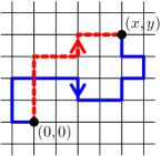
Figure 1.4: Left: An illustration of the Eden model. The dots represent occupied sites, and the arrows represent the possible ways of new occupation. Each happens with a rate $\mathrm{d}t$. Right: Two polymers from $(0,0)$ to $(x,y)=(4,4)$. The dashed red one is a directed polymer, while the blue one is undirected.

To derive the formula for $T(x,y)$ (see eq. (1.19) below), which establishes the claimed relation between the Eden model and the polymer model, consider a lattice edge $\mathsf{e}:(x,y)-(x^{\prime},y^{\prime})$ connecting the two sites, and assume $(x^{\prime},y^{\prime})$ is occupied before $(x,y)$. According to the dynamics rule, $(x,y)$ will be occupied from $(x^{\prime},y^{\prime})$ at $T(x^{\prime},y^{\prime})+\tau(\mathsf{e})$, where $\tau(\mathsf{e})$ is the waiting time assigned to $\mathsf{e}$. The waiting time for all edges is i.i.d.. random variables, with standard exponential distribution $\mathrm{pdf}(\tau(\mathsf{e}))=e^{-\tau(\mathsf{e})}$ ($\tau(\mathsf{e})\geq 0$). Now, Remembering that $T(x,y)$ can be occupied from any of its neighbours, we have

$$T(x,y)=\min_{\mathsf{e}:(x^{\prime},y)-(x,y)}\left[T(x^{\prime},y^{\prime})+\tau(\mathsf{e})\right]\,.$$

Iterating this formula (i.e., writing $T(x^{\prime},y^{\prime})$ at the right hand side as a minimum over its neighbours, and so on), and combing with the initial condition, one concludes that $T(x,y)$ is a minimum over all the lattice paths $\mathfrak{p}:(0,0)-(x,y)$ made of a sequence of edges $e_{1},\dots,e_{s}$

$$T(x,y)=\min_{\begin{subarray}{c}\mathfrak{p}:(0,0)\to(x,y)\end{subarray}}E[\mathfrak{p}]\,,\,E[\mathfrak{p}=(\mathsf{e}_{1},\dots,\mathsf{e}_{s})]=\left[\sum_{j=1}^{s}\tau(\mathsf{e}_{j})\right]\,,$$ (1.17)

where the length of the path $s=s(\mathfrak{p})$ is not fixed. What we just obtained is a first–passage percolation (FPP) model [22, 23] corresponding to the Eden growth model. In section 3.2.2 we will see the another application of such a mapping.

Equation (1.17) expresses $T(x,y)$ as a minimum. So, we can define the finite–temperature version of it. For this, we regard $T(x,y)$ as the minimum energy of the ensemble of undirected polymers, modelled as any lattice paths connecting $(0,0)$ and $(x,y)$ in a random medium, described by the random energies $\{\tau(\mathsf{e})\}$; see Figure 1.4 (right panel) for illustration. The energy of a polymer configuration is the sum of its edge-energies. Such a model can be defined at finite temperature $T=1/\beta$, in the canonical grand-canonical ensemble, by the partition function

$$\mathcal{Z}=\sum_{\begin{subarray}{c}\mathfrak{p}:(0,0)\to(x,y)\end{subarray}}\exp\left[-\beta\sum_{j=1}^{s}(\tau(\mathsf{e}_{j})-\mu)\right]\,,$$ (1.18)

where $\mu$ is the chemical potential coupled of a monomer. Then, it is not hard to see that

$$T(x,y)=\left[-\beta^{-1}\ln\mathcal{Z}\right]_{\mu=0,\beta\to+\infty}$$ (1.19)

is retrieved as the zero temperature, zero chemical potential limit. This is the advocated relation between the Eden growth model and polymers in random media: the latter is the finite–temperature version of the FPP problem corresponding to the Eden model. Note that if the chemical potential $\mu\neq 0$, the zero–temperature limit gives a FPP model with

$$E[\mathfrak{p}=(\mathsf{e}_{1},\dots,\mathsf{e}_{s})]=\sum_{j=1}^{s}\left(\tau(\mathsf{e}_{j})-\mu\right)$$ (1.20)

instead of eq. (1.17). It is interesting to consider $\mu<0$ and $\mu>0$ separately:

• When $\mu>0$, there can be some edge such that $\tau(\mathsf{e})<\mu$. This is problematic because the polymer can visit this edge back and forth to lower its energy to $-\infty$. In statistical physics, this is well–known to be a signature of condensation, e.g. Bose–Einstein condensate. Although $\mu>0$ is forbidden in statistical physics, it does have an application when we relate the polymer model to quantum mechanics, as we shall see in sections 3.3.3 and 3.3.4.

• When $\mu<0$, this energy function punishes longer paths. In particular, when $\mu\to-\infty$, one obtains the directed polymers in random media model, whose partition function sums over only lattice paths of minimal length $s=s_{\min}=\left|x\right|+\left|y\right|$ (see the dashed line in Figure 1.4, right panel for an example):

  $$\mathcal{Z}_{\text{DP}}=\sum_{\begin{subarray}{c}\mathfrak{p}:\mathsf{e}_{1},\dots,\mathsf{e}_{s_{\min}}\\ (0,0)\to(x,y)\end{subarray}}\exp\left[-\beta\sum_{j=1}^{s_{\min}}\tau(\mathsf{e}_{j})\right]\,.$$ (1.21)

  Moreover, it is also well-known that (see e.g., [19]), with the time coordinate $t=x+y$ and space coordinate $u=x-y$, the free energy satisfies the KPZ equation, in an appropriate scaling regime. Now, we can now argue the undirected polymer model defined by eq. (1.18) is also described by KPZ in the continuum limit, since the dominant contribution to $\mathcal{Z}$ comes from polymers that are directed in the large scale.

The major concrete consequence of “belonging to the KPZ class” is the following prediction. For $(x,y)=(r\cos\theta,r\sin\theta)$ far from $(0,0)$ ($r\to\infty$), $T(x,y)$ satisfies the following version of Ansatz eq. (1.2)

$$T(r\cos\theta,r\sin\theta)\stackrel{{\scriptstyle r\to\infty}}{{\longrightarrow}}ra(\theta)+r^{\frac{1}{3}}b(\theta)\chi\,,$$ (1.22)

where $\chi$ obeys a Tracy–Widom distribution [24] . Another universal signature is the scaling $r^{\frac{1}{3}}$. On the other hand, the pre–factors $a(\theta)$ and $b(\theta)$ are not universal and depend on the microscopic details of the model. In particular, $a(\theta)$ is directly related to the limit shape of the Eden model, so is unknown. The finite–temperature energy $-\beta^{-1}\mathcal{Z}$ (for $\mu\geq 0$) is also expected to have the scaling form eq. (1.22) with different $a(\theta)$ and $b(\theta)$ but the same exponent $r^{1/3}$ and distribution $\chi$.

Remarkably, eq. (1.22) describes another problem of extreme value statistics in random matrix theory [25]: for a large class of random matrices of si $N\times N$, as $N\to\infty$, the largest eigenvalue $\lambda_{\min}$ limiting distribution $\lambda_{\min}=a\sqrt{N}+bN^{1/6}\chi$; it can be matched with eq. (1.22) by setting $N=r^{2}$. This is not a coincidence, but there is a deep connection. In fact, using ingenious combinatorial methods, it has been shown [26] that, $\lambda_{\min}$ could be closely related to a cousin to the first–passage percolation problem, the last–passage percolation, whose finite–temperature version is in turn the directed polymer in random media model (eq. (1.21))!

The fact that the same universality governs seemingly unrelated phenomena makes KPZ a fascinating subject, and the various related models are extensively studied. Although this thesis contains no direct contribution to KPZ in finite dimensions, let us mention the following:

• The directed polymer model can be defined in any dimension, and also on a Cayley tree. That case turns out to be an important case , for several reasons: it can be exactly analysed [27]; it corresponds to KPZ in $d=\infty$ dimension; moreover, it is also a logREM (see section 2.1.2)! In fact it was the first logREM ever studied, before those defined by log-correlated random potentials in Euclidean spaces (e.g., the one in section 1.2). As we shall see in Chapter 2, the remarkable close relation between a $d=\infty$ model and finite dimensional ones is the essential reason behind the applicability of replica symmetry breaking (RSB), a disordered–systems method usually limited to mean-field models, to finite-dimension logREM.

• KPZ universality also appears in Anderson localization, which we study in Chapter 3. It is a well–known quantum mechanical phenomenon of a particle in a random potential. Its relation to the classical statistical physics of the directed polymer in random media problem was realized during the early days of KPZ [28, 29], and turned out quite fruitful up to now. We shall revisit this in section 3.3.4.

Chapter 2 Log-correlated Random Energy Models

2.1 History and background

This section reviews the theoretical backgrounds that lead to the field of logarithmically correlated Random Energy Model (logREM). Section 2.1.1 is a quite detailed introduction to the Random Energy Model (REM), covering its freezing transition and free energy distribution. Section 2.1.2 introduces the directed polymers on the Cayley tree (DPCT) model, which is the first logREM. Section 2.1.3 reviews the key developments of logREM on Euclidean spaces, including works of Mudry et. al. and of Carpentier–Le Doussal, the circular model of Fyodorov–Bouchaud, and the freezing duality conjecture. Section 2.1.4 introduces the basic multi–fractal properties of logREM, and the transitions associated.

2.1.1 Random Energy Model (REM)

The Random Energy Model has been introduced in Chapter 1 as the finite temperature version of a simple extreme value statistics problem. The genuine motivation of Derrida [8, 30] was to design a simple toy model of spin glass. Since the classic work of Edwards and Anderson [31], spin glass is associated with the Ising model with random interaction, whose partition function (at zero magnetic field) is

$$\mathcal{Z}=\sum_{\sigma_{1}=\pm 1}\dots\sum_{\sigma_{N}=\pm 1}\exp(-\beta H[\sigma_{1},\dots,\sigma_{N}])\,,\,H[\sigma_{1},\dots,\sigma_{N}]=\sum_{<ij>}J_{ij}\sigma_{i}\sigma_{j}\,,\,$$ (2.1)

where $\beta$ is the interaction, $\sum_{<ij>}$ sums over neighbouring pairs in a lattice, and $J_{ij}$’s are random couplings: usually, they are taken as independent and identically distributed (i.i.d.) Gaussian with variance $1/N$, so that

$$\overline{H[\sigma_{1},\dots,\sigma_{N}]^{2}}\propto N\,.$$ (2.2)

The model defined by eq. (2.1) turned out to be significantly more difficult than its non–disordered cousin. It is still poorly understood in three dimensions. The solution of the mean field version, defined on a fully connected network, was a heroic effort, and involved the invention of new theoretical insights and methods: the replica trick initiated by Sherrington and Kirkpatrick [32], the de Almeida–Thouless stability [33], which led to the discovery of replica symmetry breaking, accumulating in the Parisi’s tour–de–force exact solution [34, 35]. The complete story, as well as the foundational papers, can be found in Part one of classic book [9] (other textbooks include [10]; mathematicians may prefer [36]).

A striking feature of the spin–glass theory is its non-rigorousness: both the replica trick and the replica symmetry breaking (RSB)involve manipulations which would shock any mathematician. The REM was the first step in the mathematical development of spin–glass theory. For this, Derrida tremendously simplified the model eq. (2.1). It retains two features of eq. (2.1) and (2.2): the partition function sums over an exponential number $M=\exp(cN)$ of configurations, and the energy of each configuration has variance $\propto N\propto\ln M$. However, it neglects the correlations between energy levels. After some rescaling, one obtains the Random Energy Model (REM)partition function that we have seen in section 1.1:

$$\mathcal{Z}=\sum_{j=1}^{M}\exp(-\beta V_{j})\,,\,(V_{j})\text{ Gaussian, }\overline{V_{j}}=0\,,\,\overline{V_{i}V_{j}}=2\ln M\,\delta_{ij}\,.$$ (2.3)

By the above reasoning, we expect that the thermodynamic quantities of the REM are proportional to $\ln M$, which is the system volume of the spin glass model being mimicked.

Freezing transition

The most important fact about the REM is that it has a phase transition at $\beta=\beta_{c}$, where $\beta_{c}=1$ with the normalization of eq. (2.3). The simplest way to see it is to work in the micro–canonical ensemble (as in [8]). For this, let us fix an energy $E$. Since each energy level is a Gaussian with probability density function (pdf) $P(V_{j})=(4\pi\ln M)^{-\frac{1}{2}}\exp(-V_{j}^{2}/4\ln M)$, $j=1,\dots,M$, the (mean) number of configuration with energy $E$ is $\overline{\mathcal{N}(E)}=P(E)M$. As a consequence, $\overline{\mathcal{N}(E)}\ll 1$ when $\left|E/\ln M\right|>2$. When $E/\ln M\in(-2,2)$, $\overline{\mathcal{N}(E)}\sim M^{1-\frac{E^{2}}{4\ln M}}(4\pi\ln M)^{-\frac{1}{2}}\gg 1$. Since the energies are independent, $\mathcal{N}(E)$ has a binomial distribution, which has no algebraic (fat) tail. For such distributions, the mean value is representative of the typical value; therefore, the entropy can be estimated by

$$\frac{S(E)}{\ln M}\to\frac{\ln\overline{\mathcal{N}(E)}}{\ln M}=1-\frac{1}{4}\left[\frac{E}{\ln M}\right]^{2}\,,\,\frac{E}{\ln M}\in(-2,2)\,,\,$$ (2.4)

Using standard thermodynamics formulas, we calculate the inverse temperature $\beta=\frac{\partial S}{\partial E}=-E/(2\ln M)\in(-1,1)$, and the free energy

$$\mathcal{F}/\ln M=(E-\beta^{-1}S)/\ln M\to-\left(\beta+\beta^{-1}\right)\,,\,\left|\beta\right|<1\,.$$ (2.5)

Remark that as $\beta\to 1$, $E/\ln M\to-2$, $S/\ln M\to 0$: the entropy becomes sub-extensive at a non–zero temperature. This is a key signature of disordered systems: it is called the entropy crisis, and is responsible for their glassy behaviour and slow dynamics. What happens at lower temperatures? Since the entropy cannot further decrease and cannot increase either, the only possibility is that $S=0$, and the free energy becomes temperature independent:

$$\mathcal{F}/\ln M\to-2\,,\,\beta\geq 1\,.$$ (2.6)

From now on we restrict to $\beta\geq 0$ by default. Equations (2.5) and (2.6) imply a second–order transition at $\beta=\beta_{c}=1$, called the freezing transition. In particular, as $\beta\to\infty$, we recovers the leading term $V_{\min}=-2\ln M+\dots$ of the extreme value statistics, eq. (1.4). To recover the correction terms and the Gumbel law of the fluctuation, one may use the one–step replica symmetry breaking method, as we will discuss in section 2.3.1 below. Here, we give an elegant replica-free method (provided in [6], last appendix) to calculate the distribution of $\mathcal{F}$ at any temperature. This allows also introducing some standard formalism that will be used recurrently in this chapter.

Free energy distribution

A central quantity in disordered statistical physics is the (exponential) generating function of partition function

$$G_{\beta}(x)=\overline{\exp\left(-e^{\beta x}\mathcal{Z}\right)}\,.$$ (2.7)

It can be interpreted in several ways:

1. As the exponential generating series

   $$G_{\beta}(x)=\sum_{n=0}^{\infty}\frac{(-\mu)^{n}}{n!}\overline{\mathcal{Z}^{n}}\,,\,\mu=e^{\beta x}$$ (2.8)

   of the replicated partition sums $\overline{\mathcal{Z}^{n}}$, $n=0,1,2,\dots$: they are the object that is calculated in the replica approach. However, the series, as a function of $\mu$, has usually zero convergence radius around $\mu=0$, so eq. (2.8) is only useful for formal manipulations, for example, the differentiation

   $$\partial_{x}G_{\beta}(x)=\sum_{n=0}^{\infty}\frac{(-\mu)^{n}}{n!}n\beta\overline{\mathcal{Z}^{n}}\,.$$ (2.9)

2. As a cumulative distribution function. This is the most important interpretation, and is in fact the proper definition of eq. (2.7). To explain it, let us introduce $g$, a random variable independent of $\mathcal{Z}$ which has the standard Gumbel distribution. That is, its cumulative distribution function and Laplace transform are respectively

   $$\overline{\theta(x-g)}=\exp(-e^{-x})\Leftrightarrow\overline{e^{tg}}=\Gamma(1-t)\,,\,\Re(t)<1\,.$$ (2.10)

   where $\theta$ is the Heaviside step function and $\Gamma$ is Euler’s Gamma function. Now, eq. (2.7) implies

   $$G_{\beta}(x)=\overline{\exp\left(-e^{\beta(x-\mathcal{F})}\right)}=\overline{\theta(-\beta(x-\mathcal{F})-g)}=\overline{\theta(\left[\mathcal{F}-g/\beta\right]-y)}\,,$$ (2.11)

   i.e., the probability that the sum of $\mathcal{F}$ and an independent rescaled Gumbel $-g/\beta$ is larger than $y$. Therefore $-\partial_{x}G_{\beta}(x)$ is the pdf of the convolution $(\mathcal{F}-g/\beta)$:

   $$\overline{\delta(\mathcal{F}-g/\beta-x)}=-\partial_{x}G_{\beta}(x)\,.$$ (2.12)

   As a consequence, we have the Fourier–Laplace transform relations

   $$\int_{\mathbb{R}}(-\partial_{x}G_{\beta}(x))e^{tx}\mathrm{d}x=\Gamma(1+t/\beta)\,\overline{\exp(t\mathcal{F})}\,,$$ (2.13a)

   $$\int_{r+\mathbf{i}\mathbb{R}}\frac{\mathrm{d}t}{2\pi\mathbf{i}}e^{-tx}\,\beta^{-1}\Gamma(t/\beta)\,\overline{\exp(t\mathcal{F})}=G_{\beta}(x)\,,$$ (2.13b)

   where $r$ can be chosen such that the vertical contour $r+\mathbf{i}\mathbb{R}$ is at the right of all the poles of the integrand. Equations (2.11) through eq. (2.13b) are fundamental to follow and understand various technical aspects of this Chapter. For the engaged Reader, the best way to get familiar with them is to follow the REM case, especially, working through the details from eq. (2.23) to eq. (2.24) and from eq. (2.25) to eq. (2.27).

   Remark that, applying the residue theorem to eq. (2.13b), and assuming that $\overline{\exp(t\mathcal{F})}$ has no poles, we would obtain a formal series coming from the poles of $\Gamma(t/\beta)$ at $t/\beta=-n,n=0,1,2,\dots$:

   $$G_{\beta}(x)=\sum_{n=0}^{\infty}\frac{(-1)^{n}}{n!}e^{\beta ny}\overline{\mathcal{Z}^{n}}+\dots\,,$$

   comparable to eq. (2.8). Therefore, the integral eq. (2.13b) can be used as a non–rigorous re–summation of the series eq. (2.8), if we can continue $\overline{\mathcal{Z}^{n}}$ to complex $n$. Such manipulations are behind the replica approach, as we will see in section 2.3.

3. Finally, it is important to note that

   $$G_{\beta}(y)=\overline{\prod_{j=1}^{M}\theta_{\beta}(V_{j}-x)}\,,\,\text{where}$$ (2.14)

   $$\theta_{\beta}(x)=\exp\left(-e^{-\beta x}\right)\stackrel{{\scriptstyle\beta\to\infty}}{{\longrightarrow}}\theta(x)\,,$$ (2.15)

   i.e., $\theta_{\beta}$ is a finite temperature smearing of the Heaviside step function $\theta$. As a consequence:

   $$G_{\beta}(x)\stackrel{{\scriptstyle\beta\to\infty}}{{\longrightarrow}}\overline{\prod_{j=1}^{M}\theta(V_{j}-x)}=\overline{\theta(V_{\min}-x)}\,,$$ (2.16a)

   i.e., $$G_{\infty}(x) V_{\min} V_{\min}$$ is one minus the cumulative distribution function of . The pdf of is then obtained by derivation:

   $$-\partial_{y}G_{\infty}(x)=\overline{\delta(V_{\min}-x)}\,.$$ (2.16b)

The above discussion is completely general, and applies to any disordered statistical physics model.

For the REM (see [6], last appendix), for which $V_{j}$’s are independent, eq. (2.14) simplifies to

$$G_{\beta}(x) =\left[\gamma_{\beta}(x)\right]^{M}\stackrel{{\scriptstyle M\to\infty}}{{\longrightarrow}}e^{\hat{\gamma}_{\beta}(y)}\,,\,\hat{\gamma}_{\beta}=\lim_{M\to\infty}\left(M(\gamma_{\beta}-1)\right)\,,$$ (2.17)

$$\gamma_{\beta}(x) =\overline{\theta_{\beta}(V_{j}-x)}=\int_{\mathbb{R}}\frac{\mathrm{d}ve^{-\frac{v^{2}}{4\ln M}}}{\sqrt{4\pi\ln M}}\exp(-e^{\beta(x-v)})\,.$$ (2.18)

The last quantity can be calculated by a Hubbard-Stratonovich transform: i.e., we insert into the above equation the identity

$$\frac{e^{-\frac{v^{2}}{4\ln M}}}{\sqrt{4\pi\ln M}}=\int_{\mathbb{R}-\mathbf{i}\epsilon}\frac{\mathrm{d}p}{2\pi}e^{-pv+p^{2}\ln M}\,,\,\epsilon>0\,,$$ (2.19)

and then integrate over $v$ in terms of the Gamma function,

$$\gamma_{\beta}(x) =\int_{\epsilon+\mathbf{i}\mathbb{R}}\frac{\mathrm{d}p}{2\pi\mathbf{i}}e^{p^{2}\ln M-xp}\int_{\mathbb{R}}\mathrm{d}ve^{-p(v-x)}\exp\left(-e^{\beta(x-v)}\right)$$ (2.20)

$$=\int_{\epsilon+\mathbf{i}\mathbb{R}}\frac{\mathrm{d}p}{2\pi\mathbf{i}}e^{p^{2}\ln M-xp}\beta^{-1}\Gamma(p/\beta)$$ (2.21)

$$=1+\int_{-\epsilon+\mathbf{i}\mathbb{R}}\frac{\mathrm{d}p}{2\pi\mathbf{i}}e^{p^{2}\ln M-xp}\beta^{-1}\Gamma(p/\beta)$$ (2.22)

In eq. (2.19), the contour is at the right of the imaginary axis so that the $v$-integral in eq. (2.20) converges at $v\to+\infty$. In eq. (2.22) we move the contour across the imaginary axis, picking up the residue of the Gamma pole at $p=0$, which gives $1$ by the Cauchy’s formula.

The remaining integral shall be analysed by the saddle point/steepest descent method, the saddle point of (2.22) being at $p_{*}=x/(2\ln M)$. For this, (2.17) implies that one should consider the regime of $y$ where $\hat{\gamma}_{\beta}\sim O(1)$, or $\gamma_{\beta}\sim 1/M$. Expectedly, such regimes are in agreement with eq. (2.5) and (2.6). So the analysis is different in the two phases (see Figure 2.1 for an illustration):

Figure 2.1: Illustrations of the deformed contour integral. The Gamma poles at indicated with a cross. The residue of the pole at $0$ gives the term $1$ in eq. (2.22). Left: In the $\beta<1$ phase, the dominant contribution comes from the pole at $-\beta$. Right: In the $\beta>1$ phase, the dominant contribution comes from the saddle point at $p_{*}>-\beta$.

1. $\beta<1$. Eq. (2.5) implies the relevant regime should be $x=-(\beta+\beta^{-1})\ln M+y$, $y\sim o(\ln M)$. But then $p_{*}/\beta<-1$, so to deform the contour to cross the saddle point, one has to pick up residues of some Gamma poles. It is not hard to check that the pole at $p=-\beta$ has dominant contribution:

   $$\hat{\gamma}_{\beta}(x)=-e^{\beta y}\stackrel{{\scriptstyle\eqref{eq:GbetaREM}}}{{\Rightarrow}}G_{\beta}(y)\stackrel{{\scriptstyle M\to\infty}}{{=}}\exp\left(-e^{\beta y}\right)\,,\,x=y-(\beta+\beta^{-1})\ln M\,.$$ (2.23)

   By eq. (2.12), this means that

   $$\overline{\theta(\mathcal{F}-g/\beta-x)}=\exp(-\exp(\beta(x+(\beta+\beta^{-1})\ln M)))\,,$$

   i.e., the pdf of $\mathcal{F}-g/\beta$ is equal to that of $-g/\beta-(\beta+\beta^{-1})\ln M$ (where we recall that $g$ is a standard Gumbel random variable independent of $\mathcal{F}$). As a consequence, the free energy becomes deterministic in the thermodynamic limit:

   $$\mathcal{F}\equiv-(\beta+\beta^{-1})\ln M\,.$$ (2.24)

2. $\beta>1$. Eq. (2.6) points to the regime $x=-2\ln M+o(\ln M)$, so $p_{*}/\beta>-1$, thus no pole-crossing is needed to deform the contour to the saddle point. Yet, $x=-2\ln M$ would give $\gamma_{\beta}=1+M^{-1}(4\pi\ln M)^{-\frac{1}{2}}$, with an extra correction from the Jacobian; so the correct regime of $x$ should be $\sim-2\ln M+\frac{1}{2}\ln\ln M$. More precisely, one can check the following:

   $$G_{\beta}(x)\stackrel{{\scriptstyle M\to\infty}}{{\longrightarrow}}\exp\left(-e^{y}\right)\,,\,x=y-2\ln M+\frac{1}{2}\ln\ln M+c_{\beta}\,,$$ (2.25)

   where $c_{\beta}=\frac{1}{2}\ln(4\pi)-\ln\Gamma(1-\beta^{-1})$. It diverges at $\beta\to 1_{+}$, ensuring the matching with the $\beta<1$ phase. At the zero–temperature $\beta\to\infty$ limit, we retrieve eq. (1.4) in Chapter 1, by recalling eq. (2.16). For the sake of later comparison, we note that eq. (2.25) has an exponential tail at $y\to-\infty$:

   $$1-G_{\beta}(x)\sim e^{y}+O(e^{2y})\,,\,y\to-\infty\,.$$ (2.26)

   In terms of eq. (2.12), the equation (2.25) means that the pdf of the convolution $(\mathcal{F}-g/\beta)$ is temperature independent in the $\beta>1$ phase, up to a translation. This is a remarkable fact that further justifies calling the $\beta=1$ transition freezing: not only the extensive free energy freezes, but also its fluctuation, after convolution with $g/\beta$. It should be stressed that the free energy distribution does not freeze, because it is obtained from that of $\mathcal{F}-g/\beta$ by undoing the convolution with $-g/\beta$; in terms of moment generating function, by applying eq. (2.13a), it is not hard to see

   $$\overline{e^{t\mathcal{F}}}\stackrel{{\scriptstyle M\to\infty}}{{\longrightarrow}}\frac{\Gamma(1+t)}{\Gamma(1+t/\beta)}M^{-2t}\left(\ln M\right)^{\frac{t}{2}}e^{tc_{\beta}}\,.$$ (2.27)

A curious mathematical message of the above analysis is the following: in the $\beta<1$ phase, $\hat{\gamma}_{\beta}$ is dominated by a residue (discrete term), while in the $\beta>1$ phase, it is dominated by a saddle point integral (continuous term), which induces the $\ln\ln M$ correction. We shall observe strikingly similar patterns in the Liouville field theory, see section 2.6.

Large deviation and near-critical scaling

The remainder of this section, rather technical and detached from the rest of the manuscript, is devoted to a closer look at the REM’s near-critical regime and large deviation associated. We use the temporary notations

$$\beta=1-\tau\,,\,\left|\tau\right|\ll 1\,,\,x=-2N+\delta\,,N=\ln M\,.$$ (2.28)

We will allow $\delta$ to be potentially large (so it is to be differentiated with $y$), so as to explore the effect of atypical free energy fluctuations. As indicated above, we should focus on the competition between the saddle point at

$$p_{*}=\frac{\delta}{2N}-1$$ (2.29)

and the pole at $p=-\beta$ (we shall assume $0>p_{*}>-2\beta$ to avoid the effect of other $\Gamma$– poles). We will also concentrate on $\hat{\gamma}_{\beta}=\ln G_{\beta}$, by eq. (2.17). There are three cases:

1. $2N\tau>\delta$, $p_{*}<-\beta$, and we have the contribution of both the saddle point and the pole (the latter is sub-dominant, but will be kept here)

   $$\hat{\gamma}_{\beta}(x)=-e^{\beta\delta+N\tau^{2}}+e^{\delta-\frac{\delta^{2}}{4N}}\int_{s\in\mathbb{R}}\frac{\mathrm{d}s}{2\pi}\beta^{-1}\Gamma(p_{*}/\beta+\mathbf{i}s)e^{-s^{2}\beta^{2}N}$$ (2.30)

   $$=-e^{\beta\delta+N\tau^{2}}-e^{\delta-\frac{\delta^{2}}{4N}}\left(\frac{1}{\sqrt{4\pi N}}\frac{\Gamma(2+p_{*}/\beta)}{(p_{*}+\beta)}+O(N^{-\frac{3}{2}})\right)\,.$$ (2.31)

   This means that conditioning a left large deviation of free energy drives the system into a discrete term dominating phase, even if $\beta>1$. More generally, as $\delta\to-\infty$, one can drive the system into phases where there are more and more Gamma poles.

2. $2N\tau<\delta$, $p_{*}>-\beta$ so the pole does not contribute at all:

   $$\hat{\gamma}_{\beta}(x) =e^{\delta-\frac{\delta^{2}}{4N}}\int_{s\in\mathbb{R}}\frac{\mathrm{d}s}{2\pi}\beta^{-1}\Gamma(p_{*}/\beta+\mathbf{i}s)e^{-s^{2}\beta^{2}N}$$ (2.32)

   $$=e^{\delta-\frac{\delta^{2}}{4N}}\left(\frac{1}{\sqrt{4\pi N\beta^{2}}}p_{*}^{-1}\Gamma(1+p_{*}/\beta)+O(N^{-\frac{3}{2}})\right)\,.$$ (2.33)

   This means that right large deviation $\delta>2N\tau$ drives the system into the phase where continuous term dominates, even if $\tau>0$, that is, the typical system is in the high-$T$ phase.

3. $2N\tau=\delta$, the saddle point is exactly at the $\Gamma$-pole, giving a novel type of contribution

   $$\hat{\gamma}_{\beta}(x) =e^{\delta-\frac{\delta^{2}}{4N}}\int_{s\in\mathbb{R}-\mathbf{i}\epsilon}\frac{\mathrm{d}s}{2\pi}\Gamma(-1+\mathbf{i}s)e^{-s^{2}\beta^{2}N}$$ (2.34)

   $$=e^{\delta-\frac{\delta^{2}}{4N}}\int_{s\in\mathbb{R}-\mathbf{i}\epsilon}\frac{\mathrm{d}s}{2\pi}\left[\frac{\mathbf{i}}{s}+(\gamma_{E}-1)+O(s)\right]e^{-s^{2}\beta^{2}N}$$ (2.35)

   $$=e^{\delta-\frac{\delta^{2}}{4N}}\left[-\frac{1}{2}+\frac{(\gamma_{E}-1)}{\sqrt{4\pi N\beta^{2}}}+O(N^{-\frac{3}{2}})\right]\,.$$ (2.36)

Observe that equations (2.31), (2.33) and (2.36), written as such, cannot be matched together: this is because they concern the large deviations of the REM free energy. This is reflected by the fact that $p_{*}=\frac{\delta}{2N}-1$ is kept constant in the above cited equations. The results in the different phases diverge as $p_{*}\to 1$, and cannot be used to describe the critical regime. Denoting

$$\alpha=1+p_{*}/\beta=\frac{\delta-2N\tau}{2\beta N}=\frac{\delta}{2N}-\tau+O(\delta\tau N^{-1},\tau^{2},\delta^{2}N^{-2})\,,$$ (2.37)

the critical regime corresponds to $\left|\alpha\right|\ll 1$. In this regime, $\hat{\gamma}_{\beta}$ is given by the following integral (compare to (2.34))

$$\hat{\gamma}_{\beta}(x)e^{-\delta+\frac{\delta^{2}}{4N}}= \int_{s\in\mathbb{R}-\mathbf{i}\epsilon}\frac{\mathrm{d}s}{2\pi}\Gamma(-1+\alpha+\mathbf{i}s)e^{-s^{2}\beta^{2}N}$$ (2.38)

$$= \int_{s\in\mathbb{R}-\mathbf{i}\epsilon}\frac{\mathrm{d}s}{2\pi}\left[-\frac{1}{\alpha+\mathbf{i}s}+(\gamma_{E}-1)+O(\alpha+\mathbf{i}s)\right]e^{-s^{2}\beta^{2}N}$$ (2.39)

$$= -f\left(\alpha\beta\sqrt{N}\right)+\frac{\gamma_{E}-1}{\sqrt{4\pi N\beta^{2}}}+O(N^{-3/2})$$ (2.40)

$$f(y) =\frac{1}{2}e^{y^{2}}(\text{sgn}(y)-\text{erf}(y))=\begin{cases}\frac{1}{2}+O(y^{2})&y\to 0_{+}\\ -\frac{1}{2}+O(y^{2})&y\to 0_{-}\\ \pm\frac{1}{2\sqrt{\pi}y}+O(y^{-3})&y\to\pm\infty\end{cases}$$ (2.41)

Note that the jump at $y=0$ compensates exactly the appearance/disappearance of the discrete term in (2.31)/(2.33). Indeed, near $p_{*}=\beta$, all the three formulas (2.31), (2.33) and (2.36) can be matched in the following scaling description of the REM’s near critical free energy distribution:

$$\hat{\gamma}_{\beta}(x)=-e^{\delta-\frac{\delta^{2}}{2N}}\left[\tilde{f}(\alpha\beta\sqrt{N})+\frac{1-\gamma_{E}}{\sqrt{4\pi N\beta^{2}}}+O(N^{-3/2})\right]\,,\,\tilde{f}(y)=\frac{1}{2}e^{y^{2}}(1-\text{erf}(y))\,.$$ (2.42)

The divergence of $\tilde{f}(y)$ at $y\to-\infty$ matches exactly the appearance of the discrete term in (2.31), since $y=\alpha\beta\sqrt{N}\Rightarrow y^{2}=\beta\delta+N\tau^{2}-(\delta-\delta^{2}/(4N))$ is exactly the difference of the exponents. Equation (2.42) reveals also a scale $\sqrt{t}\alpha=1\Leftrightarrow\left|\delta-2N\tau\right|\sim\sqrt{N}$, so $\delta=0$ (centre of the distribution) is in the critical regime if $N<\tau^{-2}$, or $M<\exp(\tau^{-2})$: the finite size effect of the freezing transition is very strong.

2.1.2 Directed polymer on the Cayley tree

The REM introduced in the previous section is characterized by the total absence of correlations. They were subsequently incorporated in the generalized REM [37, 38]. The generalized REM have played decisive rôles in the mathematical development of spin glass theory; in particular, it led to the Ruelle cascade [39]. The latter describes the structure of low energy states of the mean field spin glass model, and is a pillar of its modern rigorous treatment (see [36]).

Figure 2.2: A Cayley tree of branching number $\kappa=2$ and $n=5$. Two directed polymers are drawn in bold and different colours. They have common length $\hat{\mathsf{q}}=2$, and overlap $\mathsf{q}=.4$. On the right panel, a sample of the energies of the directed polymers is plotted.

Another important correlated variant of REM is the directed polymers on the Cayley tree (DPCT)model, mentioned in section 1.3. It is defined on a Cayley tree (see Figure 2.2 for an illustration), described by its branching number $\kappa$ and the number of generations $n\in\mathbb{N}$, so that the total number of leaves is $M=\kappa^{n}$. To each edge, we associate an independent energy, which is a centred Gaussian variable of variance $2\ln\kappa$. Directed polymer (DP) are by definition the simple path from the tree root to one of the leaves, and its energy $V_{i},i=1,\dots,M$ is the sum of those of its edges. Therefore, the energy of each individual DP is a centred Gaussian with variance $n\times 2\ln\kappa=2\ln M$, identical to the REM, eq. (2.3); moreover, the correlation of any two DP’s is

$$\overline{V_{i}V_{j}}=2{\hat{\mathsf{q}}}_{ij}\ln\kappa\,,$$ (2.43)

where $\hat{q}_{ij}$ is the common length of the DP’s $i$ and $j$. For example, the matrix for $\kappa=2$ and $n=2$ is

$$\left(\hat{\mathsf{q}}_{ij}\right)=\begin{pmatrix}2&1&0&0\\ 1&2&0&0\\ 0&0&2&1\\ 0&0&1&2\\ \end{pmatrix}\,.$$ (2.44)

A closely related quantity is the overlap, defined by a simple rescaling:

$$\mathsf{q}_{ij}\stackrel{{\scriptstyle\text{def.}}}{{=}}\frac{\overline{V_{i}V_{j}}}{2\ln M}=\frac{\hat{\mathsf{q}}_{ij}}{n}\in[0,1]\,.$$ (2.45)

The overlap is an important notion of the spin glass theory: its definition depends on the model, so as to measure the “similarity” of two configurations (in the Ising model eq. (2.1), it is defined as $q_{\sigma,\sigma^{\prime}}=N^{-1}\sum_{j}\sigma_{j}\sigma^{\prime}_{j}\in[-1,1]$). For logREM, the first equality of eq. (2.45) will be used in general, while the second equality is specific to the DPCT model.

Branching Brwonian motion (BBM) and Kolmogorov–Petrovsky–Piscounov (KPP) equation

Figure 2.3: Left: An illustration of the BBM model. The energy levels $V_{i}$ split at rate $1$ and do independent Brownian motions such that $(\mathrm{d}V_{i})^{2}=2\mathrm{d}t$. We indicate by different colours the two families of energy levels separated at the first split. Right: Illustration of the KPP equation. The solution is a travelling wave of velocity $v<0$ and of a profile $g(y)$ given by eq. (2.51).

The DPCT is considerably more involved to study analytically than the REM. A natural idea [27], which is particularly efficient for problems defined on trees, is to consider the evolution of the directed polymer’s energy levels $V_{j}$ as one adds a generation $n\to n+1$. In one “time–step”, every level $V_{j}$ splits into $\kappa$ degenerate ones, and then each new level is incremented by an independent centred Gaussian of variance $2\ln\kappa$. It is not hard to see that the resulting energies are a sample of the DPCT with $(n+1)$ generations. This description makes clear the affinity of the DPCT to the BBM model, which we defined now. In this continuous space-time model, each energy level does an independent 1d Brownian motion with $\mathrm{d}V_{i}\mathrm{d}V_{j}=2\mathrm{d}t\delta_{ij}$, and branches into two identical copies with rate $\mathrm{d}t$. At $t=0$, there is only one energy level at $0$; therefore, at time $t$, there are in average

$$M=\overline{M(t)}=e^{t}$$ (2.46)

energy levels. So for BBM, the thermodynamics quantities should be proportional to $\ln M=t$. At time $t$, each energy level is a centred Gaussian of variance

$$\overline{V_{j}^{2}}=2t\sim 2\ln M\,,$$ (2.47)

and $\overline{V_{i}V_{j}}$ is $2$ times the branching moment of their common ancestor. Therefore, defining $\mathcal{Z}=\sum_{j=1}^{M(t)}e^{-\beta V_{j}}$ for the BBM, it is reasonable to expect that its statistical physics is close to that of DPCT, defined by $\mathcal{Z}=\sum_{j=1}^{M=\kappa^{n}}e^{-\beta V_{j}}$.

The key finding of [27] is that for BBM, the function $G(x,t)=G_{\beta}(x)=\overline{\prod_{i=1}^{M(t)}\theta_{\beta}(V_{j}-x)}$ (eq. (2.14), depending now on $t$) satisfies the Fisher-KPP equation [40] equation:

$$\partial_{t}G=\partial_{x}^{2}G+G^{2}-G\,,\,$$ (2.48a)

$$G(x,0)=\theta_{\beta}(-x)=\exp(-e^{\beta x})\,.$$ (2.48b)

We outline the reasoning leading to this. To calculate $\mathrm{d}G=G(x,t+\mathrm{d}t)-G$, we enumerate what can happen during $(0,\mathrm{d}t)$ to the only energy level:

• it moves to $\pm\sqrt{\mathrm{d}t}$ with probability $\mathrm{d}t$ (for each sign), in which case $\mathrm{d}G=\mp\sqrt{\mathrm{d}t}\partial_{x}G+\frac{1}{2}\mathrm{d}t\partial_{xx}G$ (by Itô’s calculus);

• it splits into two copies with probability $\mathrm{d}t$, in which case, by independence of the two sub–trees, $\mathrm{d}G({t+\mathrm{d}t},y)=(G^{2}-G)\mathrm{d}t$.

Summing all the contributions gives eq. (2.48a). In fact, the above reasoning shows the well known fact that for any function $\phi(y)$, the observable of the BBM

$$G_{\phi}(y)=\overline{\prod_{j=1}^{M(t)}\phi(V_{j}(t)-y)}$$ (2.49)

satisfies eq. (2.48a). Only the initial condition depends on the particular form of $\phi=\theta_{\beta}$, which is the only place where $\beta$ enters in into the KPP equation. Finally, remark that a similar recursion reasoning can be applied to DPCT. The result would be a discrete version of eq. (2.48), to which the discussion below still applies mutatis mutandis, yet much less elegantly.

REM vs. BBM

The Fisher–KPP equation is one of the best understood non-linear partial differential equations. It is one of the first examples of a reaction–diffusion model. More concretely, we will interpret KPP as a population dynamics model, in which $\rho=1-G$ is the local population density. The dynamics is a combination of (i) a uniform spatial diffusion of individuals and (ii) a local Logistic–equation dynamics $\dot{\rho}=\rho(1-\rho)$ describing an exponential reproduction which saturates at the stable fixed point $\rho=1$ (the other fixed point $\rho=0$ is unstable). In the initial condition eq. (2.48b), the right half-line is populated. It is known that the colony will invade the left-half in a travelling wave fashion, i.e., the solution in the long–time limit is of the form

$$G_{\beta}(x)=G(x,t)=g(x-a(t))\,,\,a(t)=vt+o(t)\,,$$ (2.50)

where $a(t)$ gives the leading, $t$-depending, behaviour of the free energy distribution, $v<0$ is the velocity of the travelling wave, and the wave profile $g(x)$ satisfies the ordinary differential equation, which is obtained by plugging the above eq. (2.50) into eq. (2.48a)

$$vg^{\prime}+g^{\prime\prime}+g^{2}-g=0\,,g(-\infty)=1\,,\,g(+\infty)=0\,.$$ (2.51)

It is not hard to show that the above equation with the limit conditions determines $g$ uniquely up to a global translation (a way to proceed is to interpret eq. (2.51) as Newtonian dynamics). A crucial and non–trivial part of the KPP theory is the velocity selection, i.e., determining $v$ by the initial condition. In the BBM context, by eq. (2.48b) and eq. (2.11), this amount to determining the free energy density $v=\lim_{t\to\infty}\mathcal{F}/t=\lim_{M\to\infty}\mathcal{F}/\ln M$ as a function of temperature $\beta$. The result is however surprisingly simple: it is identical to the REM, eq. (2.5) and (2.6):

$$\frac{\mathcal{F}}{\ln M}\to v=\begin{cases}-(\beta+\beta^{-1})\,,\,&\beta<1\,,\\ -2\,,\,&\beta\geq 1\,.\end{cases}$$ (2.52)

From a KPP–travelling wave point of view, behind the two cases above are two distinct velocity selection mechanisms. In fact, $v$ is selected by the left tail of the initial condition alone. Now, recall from eq. (2.48b) that, $1-G(x,t=0)=\rho(x,t=0)=1-\exp(-e^{\beta x})=e^{\beta x}+O(e^{2\beta x})$ as $x\to-\infty$. The dynamics in the regime where $\rho(x,t)\ll 1$ can be approximated by the linearization of KPP eq. (2.48a): $\rho_{t}=\rho_{xx}+\rho+O(\rho^{2})$, which can be solved by Fourier transform (just as the text-book solution of the diffusion equation). The result is

$$1-G(x,t)=\rho(x,t)\approx -e^{t}\int_{\mathbf{i}\mathbb{R}-\epsilon}\frac{\mathrm{d}p}{2\pi\mathbf{i}}e^{-px+p^{2}t}\beta^{-1}\Gamma(p/\beta)+O(\rho^{2})\,,$$ (2.53)

which is strikingly similar to the REM analysis, e.g., eq. (2.22). Therefore, eq. (2.52) can be understood by repeating the discrete (residue) vs. continuous (saddle point) argument used for the REM. This is not only a coincidence: a KPP treatment of the REM has been done in [11], section III.D.2, and the resulting equation is exactly eq. (2.53), with no further non–linearity.

Going back to statistical physics, eq. (2.52) implies that the BBM and the REM share the same thermodynamics (leading behaviour of free energy); in particular, both have a freezing transition at $\beta=1$. Moreover, eq. (2.52), (2.51) and (2.50) implies that the $t\to\infty$ limit profile of $G_{\beta}(x)$ freezes (is $\beta$-independent) in the whole $\beta>1$ phase: recall that REM has also this feature, see eq. (2.25).

Then, what are the differences between BBM and REM ? Concerning the free energy distribution, there are two essential ones: the left tail of the limit shape and the log–correction to the extensive behaviour. As we shall see in section 2.1.3, they are important universal signatures of the logREM class. So a more detailed review is in order.

$\left|y\right|e^{y}$ left tail of the limit shape

For the BBM, the limit profile of $G_{\beta}(x)$, up to a translation, is given by (2.51) (with $v$ given by (2.52)), and thus different from REM’s (minus) Gumbel profile, given by eq. (2.23) and (2.25). In particular, when $\beta<1$, the BBM’s free energy has a $O(1)$ non–trivial fluctuation, in contrast to REM, eq. (2.23). When $\beta>1$, the left tail of $G_{\beta}$ is

$$1-G_{\beta}(x)=1-g(y)\sim A\left|y\right|e^{y}+\dots\,,\,x=y+a(t)\,,\,\beta>1\,.$$ (2.54)

which is different from the REM analogue $e^{y}$, see eq. (2.26). To understand this, we can look at the ODE (2.51) around $g(y)\sim 1,y\to-\infty$. The linearised equation is $v(1-g)^{\prime}+(1-g)^{\prime\prime}+(1-g)=0$, whose general solution is $Aye^{y}+Be^{y}$ when $v=-2$ (which is the case for all $\beta\geq 1$). Since the differential equation eq. (2.51) has a non–linear part, it is reasonable that the solution is always perturbed out of the 1d manifold $\left\{A=0\right\}$ and must have $A\neq 0$. This gives us eq. (2.54).

Log–correction

The sub–leading correction to eq. (2.50) is also different from the REM. Indeed, a classic result in KPP theory is:

$$G_{\beta}(y+a(t))\stackrel{{\scriptstyle t\to\infty}}{{\longrightarrow}}g(y)\,,\,a(t)=\begin{cases}(-\beta-\beta^{-1})t+c_{\beta}\,,\,&\beta<1\,,\\ -2t+\frac{1}{2}\ln t+c_{\beta}\,,\,&\beta=1\,,\\ -2t+\frac{3}{2}\ln t+c_{\beta}\,,\,&\beta>1\,,\end{cases}$$ (2.55)

where $c_{\beta}$ denotes some $t$–independent function of $\beta$, which is different from the REM one. Eq. (2.55) holds not only for BBM, but also for DPCT, upon replacing $t=\ln M$ (the $O(1)$ correction $c_{\beta}$ varies also and depends on the Cayley tree’s branching number). The reason behind the $\frac{3}{2}$-correction in BBM/DPCT is non–trivial. Indeed, it is the subject of a very recent study [41], which constructed a class of models that interpolates the REM ($\frac{1}{2}$ correction) and the BBM/DPCT ($\frac{3}{2}$ correction, respectively). While the original and classic treatment is Bramson’s memoirs [42], there is a short and elegant explanation found recently by [43]. The key point is that the solution to the linearised KPP, eq. (2.53), is qualitatively wrong when for $x>a(t)$. For the true solution, $\rho=1-G$ becomes a constant in that regime (see Figure 2.3). To reproduce this qualitatively while keeping the approximating equation linear, one considers the same diffusion equation, but with Dirichlet boundary condition along the line $\rho(-2t+C,t)=0$ (with $C>0$ large but fixed). Such an equation can be solved by combining a shift of the reference frame and a mirror image trick; one can check that the following is a general solution:

$$\rho(-2t+C+y)=\int_{\mathbf{i}\mathbb{R}-1}\frac{\mathrm{d}p}{2\pi\mathbf{i}}e^{(p+1)^{2}t-yp}f(p)\,,\,f(-1+p)=-f(-1-p)$$

$$\approx \int_{\mathbf{i}\mathbb{R}-1}\frac{\mathrm{d}p}{2\pi\mathbf{i}}e^{(p+1)^{2}t-yp}a_{1}\times(p+1)=\frac{a_{1}ye^{y-\frac{y^{2}}{4t}}}{4\sqrt{\pi}t^{\frac{3}{2}}}\to c\left|y\right|e^{y-\frac{3}{2}\ln t}\,,$$ (2.56)

as $t\to\infty$. In the first equation of the second line, we expanded $f(p)$ around $p=-1$, $f(p)=a_{1}(p+1)+O((p+1)^{3})$, to get the leading term of the saddle point approximation. By doing this we get both the $\frac{3}{2}\ln t$ shift in the $\beta>1$ phase and the $\left|y\right|e^{y}$ tail. At the critical temperature $\beta=1$, the initial condition has an exponential tail $e^{y}$ corresponding to a pole $f(p\to-1)\sim(1+p)^{-1}$: this pole cancels the $(p+1)$ factor in eq. (2.56), and we get the $\frac{1}{2}\ln t$ correction.

As a recapitulation of the above discussions, we deduce that at the zero temperature $\beta\to\infty$ limit, the extreme value statistics problem associated to BBM/DPCT fits into the Ansatz eq. (1.2) as follows:

$$V_{\min}=-2\ln M+\frac{3}{2}\ln\ln M+c_{\beta}+y\,,\,P(y)\sim A\left|y\right|e^{y}\,,\,y\to-\infty\,.$$ (2.57)

The two distinguishing features discussed above are both manifest.

To conclude, we note the arguments leading to eq. (2.54) and (2.55) apply for a large class of KPP-type equations; for example, $G_{t}=G_{xx}+G^{k}-G$ ($k\geq 2$), which models the a BBM’s variant in which energy levels split into $k$ identical copies. Therefore, these equations are universal features of all the imaginable models similar to the BBM/DPCT.

2.1.3 From Cayley tree to 2D Gaussian Free Field

The idea of relating BBM/DPCT to a thermal particle in a log–correlated potential appeared in the study of certain disordered systems in 2D, both classical and quantum. An important classical case is the disordered XY model [44, 45, 46], while a representative in quantum mechanics is the 2D Dirac fermions in random magnetic field [47, 48, 49, 50]. In both cases, the log–correlated potential in question is the massless 2D Gaussian Free Field (GFF), which encodes essentially the quenched disorder. In turn, the freezing transition of the logREM defined by the 2D GFF, upon further ramification, has important consequences in these models. We will briefly explain this for the XY model at the end of this section, around eq. (2.73). The quantum applications are beyond the scope of this thesis, yet they are important subjects of future study, since freezing phenomena are present in a few non–conventional symmetry classes of 2D localisation transitions [51, 52, 53, 54, 55], see [56] for a review.

Let us come to define the 2D GFF, the 2D plane will be most often identified to the complex plane, with coordinates $z=x+\mathbf{i}y,z^{*}=x-\mathbf{i}y,x,y\in\mathbb{R}$. In statistical field theory, the 2D GFF $\phi(z)=\phi(x,y)$ defined by the massless quadratic action

$$\mathrm{P}[\phi(z)]\propto\exp\left(-\int_{\mathbb{C}}\frac{(\nabla\phi)^{2}}{4\pi\sigma^{2}}\mathrm{d}^{2}z\right)\,,\,$$ (2.58)

where $\mathrm{d}^{2}z=\mathrm{d}x\wedge\mathrm{d}y$ is the area element, and $(\nabla\phi)^{2}=(\partial_{x}\phi)^{2}+(\partial_{y}\phi)^{2}=\partial_{z}\partial_{z^{*}}\phi$ is the kinetic term of the massless free field action. The resulting covariance (Green function in field theory language) is logarithmic in real space

$$\overline{\phi(z)\phi(w)}=-\sigma^{2}\ln\left|z-w\right|\,,$$ (2.59)

where $\sigma^{2}$ is the coupling constant ($\sigma^{-2}$ is also known as the stiffness) that will be fixed later.

Some digression is helpful here to put the 2D GFF in larger physical contexts. Massless Gaussian Free Fields in general dimensions are the foundation of perturbative quantum/statistical field theory and a trivial fixed point of the renormalization group. Its Green function obeys power-law $\propto r^{2-d}$ except at $d=2$, where it is log–correlated. On the other hand, log–correlated Gaussian potentials can be defined on any spatial dimension, since they occur most naturally in $d=2$ as 2D GFF, or in $d=1$, either as the restriction of 2D GFF to some curve (a circle or an interval), or as the $1/f$-noise.

The 2D GFF is therefore at the intersection of log–correlated potentials and statistical field theory, and plays a central rôle in the critical phenomena in 2D statistical physics, the history of which is too long to review fairly here. With hindsight, it is clear that the log–correlation of the 2D GFF underlies the long–range order in the Berezinsky-Kosterlitz-Thouless transition [57, 58, 59], which concerns the super–fluidity in 2D. The Coulomb–gas picture that emerged have found wide applications in 2D critical models [60], and their continuum description: 2D conformal field theories [61, 62, 63]. When mathematicians began to turn these physical predictions into theorems, the 2D GFF became their favourite tool [64]: the notable cases are the Schramm (stochastic)–Loewner evolution [65, 66] and the geometry of random surfaces (2D quantum gravity) [67].

Beyond the static statistical models, 2D GFF is also the stationary state of the $(2+1)$-d random interface growth described by the Ewdards-Wilkinson equation [68] and the anisotropic Kardar–Parisi–Zhang (KPZ) equation [69, 70, 71, 72], which found recent application in out–of–equilibrium super–fluidity [73].

Figure 2.4: A sample of the 2D GFF, regularized on a lattice on a square torus (periodic boundary condition), with $M=2^{16}$; the image is compressed so there are less visible pixels.

2D logREM

Let us now come back to the problem of a thermal particle in a 2D GFF potential. One can write down the partition function

$$Z=\int_{\mathbb{C}}\mathrm{d}^{2}ze^{-\beta\phi(z)}\,,\,$$ (2.60)

but it is only formal, mainly because it is well-known that the 2D GFF, eq. (2.59), has divergences at both short distances and long distance. Both should be regularized to make the model properly defined. The simplest way to do this is to discretize the 2D GFF on a toroidal square lattice of size $R\times R$, and of lattice spacing $\epsilon$. Then the field can be generated by a 2D analogue of eq. (1.8)

$$\phi(x+\mathbf{i}y)=\Re\sum_{q=-L/2}^{L/2-1}\sum_{p=-L/2}^{L/2-1}\exp\left[2\pi\mathbf{i}\left(\frac{qx}{R}+\frac{py}{R}\right)\right]\mathsf{N}_{p,q}\sqrt{\mu_{p,q}}\,,\,$$ (2.61)

$$\mu_{p,q}=\frac{2}{\pi(p^{2}+q^{2})}\text{ if }(p^{2}+q^{2}>0)\,,\,\mu_{0,0}=0\,.$$ (2.62)

where $\mathsf{N}_{p,q}$ are i.i.d. independent complex standard normal variables, and $x,y=0,\epsilon,2\epsilon,\dots,R-\epsilon$ are the coordinates of the lattice points, and there are $M=(R/\epsilon)^{2}$ of them. The formula eq. (2.61) is used to simulate numerically 2D GFF in this thesis. A sample is plotted in Figure 2.4. By eq. (2.61), the covariance of such a field is

$$\overline{\phi(z)\phi(w)}=4\ln\left|\frac{R}{z-w}\right|\,,\epsilon\ll\left|z-w\right|\ll R\,,$$ (2.63)

while $\overline{\phi(z)^{2}}=2\ln M+O(1)$ (a heuristic way to remember this is noting that $\overline{\phi(z)^{2}}=\overline{\phi(z)\phi(z+\epsilon)}+O(1)$). So it differs from eq. (2.59) (with $\sigma^{2}=4$) by a diverging constant $4\ln R$. This is the infra–red (IR) divergence of 2D GFF ; its rôle in logREM will be discussed in section 2.2.3. Now that we have generated a discrete potential, the discrete partition function $\mathcal{Z}$ eq. (1.5) can be defined; the thermodynamic limit is achieved by taking $M\to\infty$, i.e., $\epsilon\to 0$ and/or $R\to\infty$: since there are no other scales in the problem, the only dimensionless parameter is $R/\epsilon$.

It turns out that the resulting thermodynamics is identical to that of DPCT/BBM. In particular, the particle goes through also a freezing transition. This correspondence between DPCT/BBM and 2D GFF was first put forward (partially) in [47] by Chamon, Mudry and Wen; In fact, the DPCT–2D GFF relation extends to finer details free energy fluctuations, and can be summarized as follows:

Upon fixing the normalization $\sigma^{2}=4$, the free energy $\mathcal{F}$ of a thermal particle in a 2D GFF has the same leading and sub–leading behaviour as BBM and DPCT : $$G_{\beta}(y+F_{M})\stackrel{{\scriptstyle M\to\infty}}{{\longrightarrow}}g(y)\,,\,F_{M}=\begin{dcases}-\left(\beta+\beta^{-1}\right)\ln M\,,\,&\beta<1\,,\\ -2\ln M+\frac{1}{2}\ln\ln M\,,\,&\beta=1\,,\\ -2\ln M+\frac{3}{2}\ln\ln M\,,\,&\beta>1\,,\end{dcases}$$ (2.64a) where $g(y)$ is some $M$-independent limit shape, which depends on the regularization procedure of the model (so in general different from the BBM one), as well as $\beta$. Moreover, identically to BBM, in the $\beta>1$ phase, $g(y)$ becomes $\beta$-independent and maintains its $\beta=1$ value (freezes): $$g(y)|_{\beta>1}=g(y)|_{\beta=1}\,.$$ (2.64b) In particular, we have the asymptotic left tail $$g(y)|_{\beta\geq 1}\sim A\left|y\right|e^{y}\,,\,y\to-\infty\,.$$ (2.64c)

The above statement and a physical demonstration thereof was the content of Carpentier and Le Doussal’s work [11]. This paper applied a real-space, Kosterlitz–Thouless type renormalization group (RG) analysis to the 2D GFF problem. The similar RG was designed for the random gauge XY model in [45, 74] (see below for more history). The outcome is that $G_{\beta}(y)$ satisfies approximatively the a KPP equation, to which the general result (2.55) applies. This explains why eq. (2.55) is valid almost verbatim in the 2D GFF problem. As a consequence, the extreme value statistics of 2D GFF is also governed by eq. (2.57). We mention also that KPP–type renormalization group equations were later obtained in related quantum mechanics problems [55].

Another important point revealed by the analysis [11] is that the dimension is irrelevant for the problem of log–correlated potentials: eq. (2.64) and associated properties (freezing of the profile) hold for a log–correlated potential in any dimension, provided the potential is normalized such that the freezing temperature $\beta_{c}=1$ (see section 2.2.1, eq. (2.89)). The question of dimension dependence of logREM is also discussed in [75].

The affinities between log–correlated potentials and BBM/DPCT go beyond free energy distribution, and suggest strongly that all these models belong to a same class, which we call logREM, and which is characterized by universal properties such as eq. (2.64). The latter, in the general context of logREM, is known as the freezing scenario.

Circular model

The above results lead to an outstanding question: can we calculate the limit distribution $g(y)$ in (2.64)? For the BBM, this problem is exactly (if not explicitly enough) solved by the ODE (2.51). For the 2D GFF, regularized on a 2D domain, no exact answer is known!

Nonetheless, since we know that the freezing scenario (eq. (2.64)) holds also for log–correlated dimensions in other dimensions than $2$, we can hope to make progress in 1D. As mentioned before, a common way to construct them is to restrict the 2D GFF to some 1D curve, such as the unit circle or the interval $[0,1]$. It turns out that, in these two geometries, the limit distribution $g(y)$ can be exactly calculated, as was shown by Fyodorov–Bouchaud [14] and Fyodorov–Le Doussal–Rosso [76]. We now review the former case, called the circular model, at a formal level, with the goal of exposing the main idea of the Fyodorov–Bouchaud’s solution.

For this, let us write down the (continuous, formal) partition function of the circular model:

$$Z=\int_{0}^{2\pi}\frac{\mathrm{d}\theta}{2\pi}\exp\left({-\beta\phi(e^{\mathbf{i}\theta})}\right)\,,\overline{\phi(z)\phi(w)}=-2\left|z-w\right|\,,\,\overline{\phi(z)}=0\,.$$ (2.65)

Notice that, since the dimension changes, the normalization of eq. (2.59) is fixed to $\sigma^{2}=2$, so that $\beta_{c}=1$. Then, we proceed by the replica trick, which starts by calculating integer moments of $Z$:

$$\overline{Z^{n}} =\int_{0}^{2\pi}\prod_{a=1}^{n}\frac{\mathrm{d}\theta_{a}}{2\pi}\overline{\exp\left({-\beta\sum_{a=1}^{n}\phi(z_{a})}\right)}\,,\,z_{a}=e^{\mathbf{i}\theta_{a}}\,.$$ (2.66)

To compute this, we use the Wick theorem, which holds any Gaussian variable $V$

$$\overline{\exp(V)}=\exp\left(\overline{V}+\frac{1}{2}\overline{V^{2}}^{c}\right)\,,\,\overline{V^{2}}^{c}=\overline{V^{2}}-\left(\overline{V}\right)^{2}$$ (2.67)

applied to $V=-\beta\sum_{a=1}^{n}\phi(z_{a})$:

$$\overline{\exp(V)} =\exp\left(\frac{1}{2}\sum_{a=1}^{n}\beta^{2}\overline{\phi(z_{a})^{2}}+\beta^{2}\sum_{a<a^{\prime}}\overline{\beta\phi(z_{a})\beta\phi(z_{a^{\prime}})}\right)$$

$$=\prod_{a=1}^{n}e^{\frac{1}{2}\beta^{2}\overline{\phi(z_{a})^{2}}}\prod_{1\leq a<b\leq n}\left|z_{a}-z_{b}\right|^{-2\beta^{2}}\,.$$

In the second equation we applied (2.65). Plugging into eq. (2.66), we have

$$\overline{Z^{n}}=\int_{0}^{2\pi}\prod_{a=1}^{n}\frac{\mathrm{d}\theta_{a}}{2\pi}\prod_{a=1}^{n}e^{\frac{1}{2}\beta^{2}\overline{\phi(z_{a})^{2}}}\prod_{1\leq a<b\leq n}\left|z_{a}-z_{b}\right|^{-2\beta^{2}}\,,\,$$ (2.68)

Eq. (2.68) is a Coulomb gas integral: the $n$ replicas interact by a power law attractive force coming from exponentiating the log correlation. Now, the “self–interaction” $\overline{\phi(z)^{2}}$ is formally infinity by eq. (2.65): this is a ultra–violet (UV) divergence, which should be regularized. Nevertheless, we do not need to discuss explicitly this issue here, since in (2.68), so long as the regularized value of $\overline{\phi(z)^{2}}$ is independent of $z$, the term involving it in (2.68) can be absorbed into a re–normalization of $Z$, which is equivalent to a shift in the free energy, immaterial to the calculation of its limit distribution. So, we shall set $\overline{\phi(z)^{2}}=0$, i.e., $\phi$ is “normal ordered” in field theory term.

Now, eq. (2.68), with $\overline{\phi^{2}(z)}=0$, is known as the Dyson integral [77] (see [78] and [79] for a review on more general exactly solvable Coulomb gas integrals), and its value is exactly known:

$$\overline{Z^{n}}=\int_{0}^{2\pi}\prod_{a=1}^{n}\frac{\mathrm{d}\theta_{a}}{2\pi}\prod_{1\leq a<b\leq n}\left|z_{a}-z_{b}\right|^{-2\beta^{2}}=\frac{\Gamma(1-n\beta^{2})}{\Gamma(1-\beta^{2})^{n}}\,,\,$$ (2.69)

whenever the integral converges, i.e., when $n\beta^{2}<1$. Therefore, the moments $\overline{Z^{n}}$ of the continuous partition function only exist for $n<\beta^{-1/2}$: for any $\beta<1$, only a finite number of moments exist; for $\beta>1$, none of them exists. This leaves too little information to determine the distribution of $Z$. The key non-rigorous step of the replica trick is to analytically continue eq. (2.69) to generic value of $n\in\mathbb{C}$. By doing this, we can obtain (guess) the moment generating function of the (continuous) free energy $F=-\beta^{-1}\ln Z$ (which differs from $\mathcal{F}$ by a constant shift):

$$\overline{\exp(tF)}=\overline{Z^{-t/\beta}}=\Gamma(1+t\beta)\Gamma(1-\beta^{2})^{t/\beta}\,.$$ (2.70a)

$$\Rightarrow\, \overline{\exp(t(F-g/\beta))}=\Gamma(1+t\beta)\Gamma(1+t/\beta)\Gamma(1-\beta^{2})^{t/\beta}\,.$$ (2.70b)

The last equation is useful because by the analogue of eq. (2.13b), $$\overline{\exp(t(F-g/\beta))} -g^{\prime}(y)$$ the Laplace transform of the limit distribution ;

$$g(y)=\int_{\mathbf{i}\mathbb{R}+\epsilon}\frac{\mathrm{d}t}{2\pi\mathbf{i}t}\,e^{-ty}\,\overline{\exp(t(F-g/\beta))}\,.$$ (2.70c)

Now, the key point is that equations (2.70) hold only in the phase $\beta<1$ (and for $\Re(t)>-1/\beta$). The basic reason behind this is that the naïve continuum formalism presented just now is invalid in the $\beta>1$ phase; we shall understand this better using the one–step replica symmetry breaking approach in section 2.3. Fortunately, for our purpose here, we do not need to compute $\overline{\exp(t(F-g/\beta))}$ for $\beta>1$, because the answer will be given by the freezing scenario, eq. (2.64b), once we know $g(y)$ (or $\overline{\exp(t(F-g/\beta))}$) at $\beta=1$. However, The point $\beta=1$ is tricky, as the factor $\Gamma(1-\beta^{2})^{t/\beta}$ in eq. (2.70a) and (2.70b) diverges. Yet, this factor is of form $e^{c_{\beta}t}$, so corresponds to a first moment shift of the distribution of $F$ (and $F-g/\beta$), and can be discarded if our only goal is to determine $g(y)$ up to a translation. Doing this, and applying (2.64b) and then inverse Laplace–Fourier transform, we have

$$g(y)|_{\beta>1}=g(y)|_{\beta=1}=\int_{\mathbf{i}\mathbb{R}+\epsilon}\frac{\mathrm{d}t}{2\pi\mathbf{i}t}\Gamma(1+t)^{2}e^{-ty}=2e^{y/2}K_{1}(2e^{y/2})\,,$$ (2.71)

$K_{n}$ denoting the Bessel $K$-function. In particular, since the pole at $t=-1$ is a double one, we have the left tail $g(y)\sim A\left|y\right|e^{y},y\to-\infty$, verifying the freezing scenario prediction eq. (2.64c). Taking derivative of eq. (2.71) we have $-g^{\prime}(y)=2e^{y}K_{0}\left(2e^{y/2}\right)$, just as eq. (1.14b) in section 1.2. This is not a coincidence, since the logREM considered in section 1.2 (more precisely, eq. (1.10) with $\alpha=1$) is one way of defining properly the circular model at the discrete level. The calculation above, combined with eq. (2.64a), essentially demonstrates eq. (1.14), leaving however numerous subtle points, which will be treated in a more systematic manner in this chapter.

By observing the above derivation, we can already be convinced that the particular limit distribution, eq. (2.71), is specific to the circular model, as it comes from the Dyson integral eq. (2.69). The analogous Coulomb gas integral for the interval model would be the Selberg integral

$$\int_{0}^{1}\prod_{a=1}^{n}\mathrm{d}x_{a}\prod_{a<b}\left|x_{a}-x_{b}\right|^{-2\beta^{2}}\,,$$

whose solution and analytical continuation are different [76], leading to a distinct limit distribution. While we will not study it in this thesis, we will study how the limit distribution of the circular model is modified if the 2D GFF is put on a finite disk, in section 2.4.2.

Freezing–duality conjecture

The authors of [76] observed that, eq. (2.70b), with the factor $\Gamma(1-\beta^{2})^{t/\beta}=e^{c_{\beta}t}$ discarded, is dual. It means that $\Gamma(1+t\beta)\Gamma(1+t/\beta)$ would be invariant under the formal change of variable $\beta\to 1/\beta$; equivalently, it is a function of the variable $\beta+\beta^{-1}$. At the same time, the same quantity freezes in the $\beta>1$ phase, by Laplace transform of eq. (2.64b). Furthermore, [76] showed that the same co-existence of freezing and duality prevails when the 2D GFF is restricted on the interval $[0,1]$ instead of a circle. The analysis of the interval model requires analytically continuing the Selberg integrals [79], which are more complex cousins of the Dyson integral eq. (2.69), and we will not do it here.

Nevertheless, we have already encountered such co-existences. The first, quite trivial, example is the free energy density of the REM and the logREM,

$$-\lim_{M\to\infty}\mathcal{F}/\ln M\to\begin{cases}\beta+\beta^{-1}\,,\,&\beta<1\,,\\ 2\,,\,&\beta>1\,.\end{cases}=\includegraphics[scale={.2},valign={c}]{showfreez.eps}\,,$$ (2.72)

It is dual in the $\beta<1$ phase and freezes in the $\beta>1$ phase. Moreover, the same thing can be said for the limit shape $g(y)$ in BBM, which is determined by the equation (2.51): $g^{\prime\prime}+vg^{\prime}+g^{2}-g=0,g(-\infty)=1,g(+\infty)=0$. This equation depends only on the selected travelling wave velocity $v=\lim_{M\to\infty}\mathcal{F}/\ln M$. So the duality and freezing of $g(y)$ follow directly from that of $v$, eq. (2.72). On the other hand, notice that the same cannot be said about the uncorrelated REM : indeed, eq. (2.23) implies that $g(y)=\exp\left(-e^{\beta y}\right)$, which is not dual.

Based on the above evidences, it was put forward in [76] the freezing-duality conjecture (this name came from [80]), which we can succinctly phrase as:

In logREM, dual quantities in the $\beta<1$ phase freeze in the $\beta>1$ phase.

To this day, this conjecture is verified in all exact solvable logREM, but the reason behind has not been understood. We shall provide some rationale for it in section 2.3.3, around eq. (2.158) and eq. (2.159), and further special cases where it is checked in section 2.4. Finally, we note that the duality observed in logREM echoes those in $\beta$–random matrix theory [81] (which has been applied to study logREM, see [82, 80]) and in 2D conformal field theory [62, 83]. The latter is not merely a superficial reminiscence: as we shall see in section 2.6, logREM are closely related to the Liouville field theory (LFT).

Application: disordered XY model

With the hindsight of the freezing transition in 2D GFF, let us briefly review its application to the disordered XY model. This model was studied by Rubinstein et. al. [44] long ago, who obtained only a partially correct phase diagram. An extensive literature was devoted to its correction [84, 85, 86, 87, 88, 45, 46, 74], in which the freezing transition in 2D GFF played a central role. Let us explain this point in the simplest possible approximation (adapted from [11], appendix D), and refer to the above original works for full treatments.

Figure 2.5: A sketch of the phase diagram of the disordered XY model. The solid curves (red and blue), corresponding to $\eta=0$ in eq. (2.75), separates the low temperature phase (the bounded region below it) and the high temperature phase. The red dashed curve is the wrong prediction that misses the freezing transition, and continues analytically the red solid curve beyond its validity. In particular, it would imply a re–entrance transition indicated by the dashed arrow. The correct phase separation for $T<T_{*}$ is instead given by the blue straight line, making the re–entrance disappear.

As a warm–up, we recall that the XY model without disorder can be defined by the Hamiltonian

$$H[(\theta_{j})]=\sum_{<jk>}J\,V(\theta_{j}-\theta_{k})\,,\,V(\theta\to 0)\sim\theta^{2}\,,$$ (2.73)

where $(\theta_{j})$ is a (discrete) field of $O(2)$ spins on a 2D lattice, and $V$ is a $2\pi$–periodic function that describes the interaction between neighbouring spins (denoted by $\left<ij\right>$). This model has a Kosterlitz–Thouless transition at temperature $T=T_{\text{KT}}$: when $T>T_{\text{KT}}$, there is a proliferation of vortices (topological defects of the XY field); when $T<T_{\text{KT}}$, the vortices form bound pairs and annihilate each other, and there is a line of fixed points enjoying an algebraic quasi–long range order. A qualitative estimate of $T_{\text{KT}}$ can be obtained by comparing the energy cost of one vortex $E\sim 2J\ln(R/\epsilon)$ ($J$ is the coupling constant of XY model) and the entropy gained, $S=\ln(R^{2}/\epsilon^{2})$ (contributed by the position of the vortex). Equating $E/T_{\text{KT}}\approx S$ gives $T_{\text{KT}}\approx J$.

Now we consider the disordered XY model defined as follows,

$$H[(\theta_{j}),(A_{jk})]=\sum_{<jk>}J\,V(\theta_{j}-\theta_{k}-\sigma A_{jk})\,,\,$$ (2.74)

where $\sigma$ is the disorder strength, and $A_{jk}$ is a quenched random gauge field which is uncorrelated, and whose corresponding magnetic field is $B(z)$. As a consequence, if $\Delta\phi(z)=\sigma B(z)$ ($\Delta$ is the discrete Laplacian), $\phi(z)$ will be a 2D GFF with coupling constant $\sigma$, see eq. (2.59). Moreover, it is known that the presence of gauge field modifies the vortex energy as follows:

$$E\leadsto E^{\prime}=E\pm J\phi(z)=2J\ln(R/\epsilon)\pm J\phi(z)\,,$$

where the sign depends on the orientation of the vortex. Therefore, the partition function of configurations with one (say, positive) vortex is very close to that of a 2D logREM :

$$\mathcal{Z}=e^{-E/T}\sum_{j=1}^{M}\exp(-J\phi(z_{j})/T)\,.$$

Its leading behaviour can be easily obtained by the freezing scenario eq. (2.64), upon proper rescaling:

$$\mathcal{Z}=\left(\frac{R}{\epsilon}\right)^{\eta}\times O(1)\,,\,\eta=\begin{cases}-2J/T+\frac{1}{2}\sigma^{2}J^{2}/T^{2}+2&T>J\sigma/2\,,\\ -2J/T+2\sigma J/T&T<J\sigma/2\,,\end{cases}$$ (2.75)

where the second case corresponds to the frozen phase. The disordered XY model is in the high temperature phase if and only if vortices are favourable, i.e., $\eta>0$. The line of phase transition is thus given by $\eta=0$, and sketched in Figure 2.5. It is non–analytic at the point $\sigma=\sigma_{*}=1,T=T_{*}=J/2<T_{\text{KT}}$. Below $T_{*}$, the critical line becomes flat and given by $\sigma=\sigma_{*}$, independently of $T_{*}$: this is the manifestation of freezing transition in the XY context (a similar phase diagram can be found in the binding transition of logREM, see section 2.3.4 and in particular, Figure 2.13). If the freezing transition had been overlooked, one would have continued the $T>J\sigma/2$ expression in eq. (2.75) beyond its scope of validity, and predict wrongly a re–entrance transition for $\sigma<\sigma_{*}$, as shown in Figure 2.5. Therefore, identifying the free transition is essential to the correct qualitative understanding of the disordered XY model’s phase diagram.

We end this discussion by warning the Reader that the above explanation does not represent accurately the rich physical questions involved the disordered and non–disordered XY models. A faithful treatment of either would require the formalism of Kosterlitz–Thouless renormalization group [59], and its disordered extension [45, 74]. From a logREM point of view, the disordered XY model can be seen as that of interacting thermal particles in a log–correlated potential, and is thus considerably more involved than logREM !

2.1.4 Multi-fractality of logREMs

Another universal feature believed to be shared by logREM (and also by the REM, but to a limited extent), is their multi–fractal properties. In fact, these are the main focus of the pioneering work [47, 48]. Multi–fractality appears in different contexts of physics, e.g., turbulence, random geometry, and critical wave-functions in Anderson transitions [56]. For the logREM, multi–fractality will refer to that of the normalized Gibbs measure:

$$p_{\beta,j}=\frac{1}{\mathcal{Z}}e^{-\beta V_{j}}\,,\,j=1,\dots,M\,,\,\mathcal{Z}=\sum_{j=1}^{M}e^{-\beta V_{j}}\,.$$ (2.76)

Figure 2.6: Left: The log-scale colour plot of the Gibbs measure of a logREM of 2DGFF on a torus.

As we can see in figure 2.6, $p_{\beta,j}$’s magnitude spans a large range. The multi–fractal spectrum of $p_{\beta,j}$ is defined by making a histogram of $-\frac{\ln p_{\beta,j}}{\ln M}$, and then “plot” it the log scale:

$$f(\alpha)=\frac{1}{\ln M\mathrm{d}\alpha}\ln\left|\left\{j:-\frac{\ln p_{\beta,j}}{\ln M}\in[\alpha,\alpha+\mathrm{d}\alpha]\right\}\right|\,,\alpha\geq 0\,$$ (2.77a)

$$\Leftrightarrow \left|\left\{j:p_{\beta,j}\sim M^{-\alpha}\right\}\right|=M^{f(\alpha)}\times\text{corrections,}$$ (2.77b)

where $\left|X\right|$ denotes the number of elements in the set $X$. In the above equations, $f(\alpha)$ is defined for any sample of disorder $(V_{j})$. However, as $M\to\infty$, $f(\alpha)$ is expected to become deterministic, and is called the multi–fractal spectrum. Note that the definitions eq. (2.77) applies to any long sequence of positive numbers $p_{j},j=1,\dots,M$. In quantum mechanics applications, they are usually the occupation probabilities of a wave function on a lattice, $p_{j}=\left|\langle j|\psi\rangle\right|^{2}$; in general, the multi–fractal spectrum is an important measure of critical wave functions, i.e., those appearing at Anderson/quantum Hall transitions [56].

For the REM and logREM, $f(\alpha)$ is quadratic [47]:

$$f(\alpha)=\frac{4(\alpha_{+}-\alpha)(\alpha-\alpha_{-})}{(\alpha_{+}-\alpha_{-})^{2}}\,,\alpha_{-}=\begin{cases}(1-\beta)^{2}&\beta<1\,,\\ 0&\beta\geq 1\,,\end{cases}\;\alpha_{+}=\alpha_{-}+4\beta\,,$$ (2.78)

see figure 2.6 for plots in the two phases. Note that the freezing transition manifests itself also in the non-analytic $\beta$-dependence of $f(\alpha)$ at $\beta=1$.

A simple derivation of eq. (2.78) goes as follows. By eq. (2.76), $\alpha_{j}=\beta(V_{j}-\ln\mathcal{F})/\ln M$. Now since $\mathcal{F}/\ln M$ is deterministic as given by eq. (2.72), and $V_{j}$ is a centred Gaussian of variance $2\ln M$. So when $M\to\infty$, $\alpha_{j}$ is a Gaussian of mean $\beta^{2}+1$ and variance $2\beta^{2}/\ln M$. Therefore, the normalized probability distribution of $\alpha$ is

$$\ln\mathrm{P}(\alpha)=\begin{dcases}-\frac{(\alpha-\beta^{2}-1)^{2}}{4\beta^{2}}+o(\ln M)\,,\,\\ -\frac{(\alpha-2\beta)^{2}}{4\beta^{2}}+o(\ln M)\,.\end{dcases}$$ (2.79)

Plugging this into $f(\alpha)=\frac{1}{\ln M}\ln\left(M\mathrm{P}(\alpha)\right)$ gives eq. (2.78) after some algebra. The tacit assumption behind the above reasoning is that the correlation between $(V_{j})$ and $\mathcal{F}$ has no effect on $f(\alpha)$. Indeed, as we will see later (section 2.6.6), the effect of the correlations are limited to the sub–leading order.

Inverse participation ratio (IPR)

The (generalized) inverse participation ratio (IPR) are important observables closely related to the multi–fractal spectrum. They are widely used in quantum mechanics to detect localization transitions (see section 3.3.4 below). For a statistical model, the IPR are defined in terms of its Gibbs measure $p_{\beta,j},j=1,\dots,M$, as follows:

$$P_{q}=\sum_{j=1}^{M}p_{\beta,j}^{q}\,,\,q\geq 0\,.$$ (2.80)

IPR for $q<0$ are seldom considered. This definition is as general as the multi–fractal spectrum: in particular, it can be calculated for each disorder realization. In the large system $M\to\infty$ limit, we can compute its leading behaviour using the definition of the multi–fractal spectrum eq. (2.77), and the saddle point approximation

$$P_{q}=\int_{I}\mathrm{d}\alpha\,M^{-q\alpha+f(\alpha)} =M^{-\tau_{q}}\times\text{corrections}\,,\,$$ (2.81)

$$\text{where }\tau_{q} =\min_{\alpha\in I}\left[q\alpha-f(\alpha)\right]\,.$$ (2.82)

Here, $\tau_{q}$ is called the multi–fractal exponent. As a function of $q$, it is calculated as the Legendre transform of the multi–fractal spectrum $f(\alpha)$, eq. (2.82). In general, it is calculated by solving the equation $\partial_{\alpha}f(\alpha_{q})=q$ for $\alpha_{q}$. The solution is unique if Since $f(\alpha)$ is convex. Thi is the case for logREM, see eq. (2.78), and we have

$$a_{q}=\begin{cases}-2q\beta^{2}+\beta^{2}+1\,,\,&\beta\leq 1\\ -2q\beta^{2}+2&\beta>1\,.\end{cases}$$ (2.83)

In general, $\alpha_{q}$ has the following interpretation: the dominating contribution to $P_{q}$ comes from those points $p_{\beta,j}\sim M^{-\alpha_{q}}$. When $q$ increases, $\alpha_{q}$ decreases. In terms of $\alpha_{q}$, the multi–fractal exponent is given as $\tau_{q}=q\alpha_{q}-f(\alpha_{q})$. After simple algebra, one finds for the logREM :

$$\tau_{q}=q\beta\left(Q-q\beta\right)-1\,,\,Q=\begin{cases}\beta+\beta^{-1}&\beta\leq 1\,,\\ 2&\beta>1\,.\end{cases}$$ (2.84)

The above notation is suggested by the Liouville field theory, see section 2.6.

The careful reader must have noticed that a crucial point has been left unexplained: what is the domain $I$ of the integral and the minimum? Indeed, if $\alpha_{q}\notin I$, eq. (2.84) would be wrong! In fact, $I$ depends on whether $P_{q}$ is calculated in the typical or annealed ensemble ([53], see [56], section II.C.7 for a review). Such difference is omnipresent in disordered systems, and arises for quantities like $P_{q}$, which can fluctuate strongly from one disorder realization to another, and has a disorder–induced pdf $P(P_{q})$. The latter has often fat (algebraic) tails, coming from rare samples; as a result, its mean value may be different from its typical value (another example for which this is the case is the partition function $\mathcal{Z}$). Therefore, it is crucial to discuss which observable of the distribution of $P_{q}$ is being calculated, i.e., specifying the ensemble:

Figure 2.7: Left: illustration of the $\alpha_{-}$–dominance transition in the typical ensemble, see eq. (2.85). The multi–fractal spectrum is not defined when $f(\alpha)<0$. Right: illustration of the termination point transition in the annealed ensemble, see eq. (2.86). The multi–fractal spectrum is defined until $\alpha=0$.

• The typical ensemble (Figure 2.7, left) concerns the typical value of $P_{q}$; in most cases, it is equivalent to the quenched ensemble $\exp\overline{\ln P_{q}}$. But here it is more helpful to think of one large typical sample of $(p_{\beta,j}),j=1,\dots,M$; their logarithms are distributed as described by $f(\alpha)$. The definition eq. (2.77) implies that when $f(\alpha)<0$, there are $M^{f(\alpha)}\ll 1$ points $j$ such that $p_{\beta,j}\sim M^{-\alpha}$: such points are absent in one large typical sample; so $I=\{\alpha:f(\alpha)\geq 0\}=[\alpha_{-},\alpha_{+}]$, see eq. (2.78). Eq. (2.84) holds in the typical ensemble only when $\alpha_{q}\geq\alpha_{-}$ in eq. (2.83), i.e., $q\leq q_{c}=f^{\prime}(\alpha_{-})=\beta^{-1}$ (in the two phases). When $q>\beta^{-1}$, the value $\alpha_{q}$ used in eq. (2.82) should not replaced by $\alpha_{q}^{\text{typ}}=\alpha_{-}$. In summary, the typical ensemble exponents are

  $$\tau_{q}^{\text{typ.}}=\begin{dcases}q\beta\left(Q-q\beta\right)-1\,,&q<\beta^{-1}\,,\\ q\alpha_{-}\,,&q\geq\beta^{-1}\,.\end{dcases}$$ (2.85)

  The non-analyticity at $\tau_{q}^{\text{typ.}}$ is referred to differently in the literature: “freezing” in [56], “pre–freezing” in [11], “$\alpha_{-}$–dominance” in [89]. We will use the last name since the other two will refer to other transitions in this work.

• The annealed ensemble (Figure 2.7, right) concerns the mean value $\overline{P_{q}}$, averaged over all disorder samples. So, even if $f(\alpha)<0$, Gibbs measure values $p_{\beta,j}\sim M^{-\alpha}$ will be present in some rare samples, and the above transition is absent: eq. (2.84) is true beyond $q=\beta^{-1}$. However, since $p_{\beta,j}\leq 1$ by normalization, so $\alpha$ can never be negative. Therefore, when $q>q_{tp}=f^{\prime}(0)=Q/(2\beta)$ (in the two phases, with $Q$ defined in eq. (2.88)), the value $\alpha_{q}$ given by eq. (2.83) is non-physical and should be replaced by $\alpha_{q}^{\text{ann.}}=0$. So the annealed ensemble exponents are

  $$\tau_{q}^{\text{ann.}}=\begin{dcases}q\beta\left(Q-q\beta\right)-1\,,&q<Q/(2\beta)\,,\\ Q^{2}/4-1\,,&q\geq Q/(2\beta)\,.\end{dcases}$$ (2.86)

  The non-analyticity of $\tau_{q}^{\text{ann.}}$ has also different names: “termination point transition” in [56] and “pre–freezing” in [89] (beware of the confusion!). We will use the term termination point transition in this work.

The above discussion is limited to the leading behaviours (exponents). In section 2.6.6 we will explore the sub–leading corrections: in particular, in the annealed ensemble, they will be predicted for the first time using Liouville field theory.

2.2 What are logREMs?

2.2.1 General characterization

In section 2.1.2 and 2.1.3, we have reviewed logREM defined on hierarchical lattices and on Euclidean spaces of different dimensions. Despite apparent differences, they share many key properties, which invite the following questions: what is common in their definition? Can we give a unifying characterization? Clearly, all logREM are defined by Gaussian energy levels $V_{j},j=1,\dots,M$. Therefore, they are completely determined by the mean values $\overline{V_{j}},j=1,\dots,M$ and the covariance matrix

$$\overline{V_{j}V_{k}}^{c}\stackrel{{\scriptstyle\text{def.}}}{{=}}\overline{V_{j}V_{k}}-\overline{V_{j}}\times\overline{V_{k}}\,,\,j,k=1,\dots,M\,.$$ (2.87)

This matrix cannot be arbitrary, and must reflect the “logarithmic correlations”. How to translate this term into a quantitative language? A simple proposal, given in [6], section II, is to look at histograms of the covariances $\overline{V_{j}V_{k}}^{c}$ with $j$ fixed, similarly to the definition of multi–fractal spectrum, eq. (2.77).

In this thesis, we normalize all the logREM so that the freezing temperature $\beta_{c}=1$. Then, for both hierarchical logREM and Euclidean space ones, the following holds:

$$\forall j\,,\,\left|\left\{k:\overline{V_{j}V_{k}}^{c}\geq 2\mathsf{q}\ln M\right\}\right|\approx M^{1-\mathsf{q}}\,,\,\mathsf{q}\in(0,1)\,.$$ (2.88)

Recall from eq. (2.45) that $\frac{\overline{V_{j}V_{k}}^{c}}{2\ln M}$ is the general definition of the overlap in logREM ; so the above equation says that for any fixed energy level $j$, there are $\sim M^{1-\mathsf{q}}$ levels that have overlap $\geq\mathsf{q}$ with it . In particular, setting $\mathsf{q}=1$, we require the variance $\overline{V_{j}^{2}}^{c}\approx 2\ln M$.

Let us check that eq. (2.88) is satisfied by the different logREM :

• For the DPCT defined on a Cayley tree of branching number $\kappa$ and depth $n$ so that $M=\kappa^{n}$, by (2.43), $\overline{V_{j}V_{k}}^{c}\geq 2\mathsf{q}\ln M$ if and only if the common length $\hat{\mathsf{q}}_{jk}$ is larger than $\hat{\mathsf{q}}=\mathsf{q}n$, where $n$ is the depth of the tree. For fixed $j$, this is satisfied for all $k$ belonging to a sub–tree of size $\kappa^{n-\mathsf{q}n}=M^{1-\mathsf{q}}$. The reasoning for the BBM is similar.

• For a log–correlated potential defined on a $d$-dimensional lattice made of points $\mathbf{x}_{j}\in\mathbb{R}^{d},j=1,\dots,M$, the correct normalization is

  $$\overline{V_{j}V_{k}}\approx 2d\ln\frac{R}{\left|\mathbf{x}_{j}-\mathbf{x}_{k}\right|}\,,\,\epsilon\ll\left|\mathbf{x}_{j}-\mathbf{x}_{k}\right|\ll R\,.$$ (2.89)

  where $\epsilon$ and $R$ are the UV cut–off (lattice spacing) and IR cut–off (linear size of the lattice), respectively, so that $(R/\epsilon)^{d}=M$. Then, for fixed $j$, $\overline{V_{j}V_{k}}\geq 2\mathsf{q}\ln M$ for $k$ in a $d$-dimensional ball of radius $r=R^{1-\mathsf{q}}\epsilon^{\mathsf{q}}$, containing $\sim(r/\epsilon)^{d}=M^{1-\mathsf{q}}$ points.

On the other hand, the uncorrelated REM does not satisfy eq. (2.88), because their the overlap $\overline{V_{i}V_{j}}^{c}/(2\ln M)$ can only assume two values $0$ and $1$. The right hand side eq. (2.88) would be modified to a step function $\theta(-q)$ for REM.

In section 2.3, we will see that eq. (2.88) is an essential input to the replica symmetry breaking approach to logREM. Nevertheless, we should be careful enough not to claim the unifying characterization a definition of logREM in a mathematical sense. The reason is that there is an important additional property of logREM, called ultra–metricity. We will discuss this in section 2.3.

2.2.2 IR and UV data

The general characterization (2.88) specifies only the structure of covariance matrix in the regime $0<\mathsf{q}<1$, which is responsible for the universal properties of the logREM, such as the free scenario, eq. (2.64). However, many other observables, such as the full limit distribution of the free energy, are not universal but model dependent; for example, the minimum distribution for the circular model, eq. (2.71) is different from that of BBM, given by eq. (2.51) (with $v=-2$). Moreover, in the sequel, we will be interested in other observables, e.g., second minimum and gap distribution (section 2.5), and the distribution of minima positions (section 2.6). These observables will all be model dependent; yet, in the $M\to\infty$ limit, they should not depend on all the details of the discrete model definition, i.e., $\overline{V_{j}}$ and $\overline{V_{j}V_{k}}^{c},j,k=1,\dots,M$. So what is the information relevant for calculating the above observables in the thermodynamic limit?

This question was already considered in [76]. We gave a systematic treatment of the issue in [6], concentrating on the logREM defined on Euclidean spaces. It turns out that the relevant information can be organized into two groups, called the IR and UV (limit) data, which we describe in a non–technical manner below (the complete technical description can be found in [6], section 2.1, and will be illustrated for the circular model below):

• The IR data specify what is the geometric manifold $X$ (circle, interval, 2D torus, …) on which the logREM potential $\phi(z),z\in X$ is defined, what is the mean value $\overline{\phi(z)}$, and the covariance $\overline{\phi(z)\phi(w)}$ for $z,w\in X$ are two distinct points; note that in the unit of lattice spacing, the distance between $z$ and $w$ go to infinity in the thermodynamic limit.

  We will show in section 2.3 that the IR data determine the continuum Coulomb gas integral in the replica approach of the logREM, which determines in turn the limit distribution (modulo a translation) of the free energy.

• The UV data concerns the covariance $\overline{V_{i}V_{j}}$ between lattice points separated by a finite number of lattice spacing in the thermodynamic limit.

  We will show in section 2.5 that the UV data determine the distribution of the gaps (e.g., the difference between the second and first minima).

The fact that only the two limiting scales are relevant is quite intuitive, since the scales in between are governed by the logarithmic decay eq. (2.89) and have no more freedom of model dependence. In section 2.3, we shall give further support to this intuition, using the replica approach.

Example: circular models

Figure 2.8: An illustration of the IR (left) and UV (right) covariances in the circle model. The formula in the IR limit corresponds to the $1/f$–noise case in eq. (2.93).

We now illustrate more technically the above ideas in the case of the circular models. We emphasized the plural form because several different definitions can be found in the literature [14, 76, 90, 3, 4], and our goal is to organize them in terms of UV and IR data. For the clearness’s sake, we shall denote $V_{j,M},j=1,\dots,M$ the potential values in a system of size $M$; any of the circular models can be defined by discrete Fourier transform (see also section 1.2)

$$V_{j,M}=\Re\sum_{k=-M/2}^{M/2-1}\sqrt{\mu_{\left|k\right|,M}}\exp\left(2\pi\mathbf{i}\frac{jk}{M}\right)\mathsf{N}_{k}\,,\,\mu_{0}=0\,.$$ (2.90)

$$\overline{V_{j,M}}=0\,,\,\overline{V_{i,M}V_{j,M}}=\sum_{k=-M/2}^{M/2-1}\mu_{\left|k\right|,M}\exp\left[2\pi\mathbf{i}\frac{(i-j)k}{M}\right]\,.$$ (2.91)

As shown in section 1.2, for the model to be a logREM (with the correct normalization for 1D), the Fourier modes $\mu_{k}$ should be $\sim 1/k$ for $1\ll k\ll M/2$. Again, some freedom is allowed at the two limiting scales. Here are some choices:

$$1/f \mu_{k,M}=k^{-1}\,,$$-noise model: (2.92a)

Dirichlet model: $$\mu_{k,M}=k^{-1}(1-q^{k})\,,\,\left|q\right|<1$$ (2.92b)

Long range model: $$\mu_{k,M}=\pi M^{-1}\sin^{-1}\left(\frac{\pi k}{M}\right)\,.$$ (2.92c)

The first choice will be the default one that we refer to as the circle model of $1/f$-noise. The second is related to the 2D GFF with Dirichlet boundary condition, see below and section 2.4.2; it reduces to the $1/f$-noise model at $q=0$. The last one is also what is considered in section 1.2 (the name comes from [76], section 6).

Let us consider the IR data of these models. For all of them, the underlying manifold is the unit circle, endowed with the uniform lattice $z_{j,M}=\exp\left(2\pi\mathbf{i}j/M\right)$. The IR limit of covariance is obtained by letting $i$ and $j$ depend on $M$, such that $z_{i,M}\to\xi$ and $z_{j,M}\to\eta$, $\xi\neq\eta,\left|\xi\right|=\left|\eta\right|=1$, then eq. (2.91) implies

$$\overline{V_{i,M}V_{j,M}}\stackrel{{\scriptstyle M\to\infty}}{{\longrightarrow}}\sum_{k=-\infty}^{\infty}(\xi\eta^{*})^{k}\lim_{M\to\infty}\mu_{\left|k\right|,M}=\begin{dcases}-2\ln\left|\xi-\eta\right|\,,\,&\text{$1/f$-noise},\\ -2\ln\left|\frac{\xi-\eta}{1-q\xi\eta^{*}}\right|\,,\,&\text{Dirichlet},\\ -2\ln\left|\xi-\eta\right|\,,\,&\text{long range}.\\ \end{dcases}$$ (2.93)

Therefore, the $1/f$-noise model and the long range model have the same IR data, corresponding to the restriction of the planar 2D GFF, eq. (2.59) to the unit circle. As a consequence, the long range and $1/f$-noise have the same limit distribution of free energy (modulo a $O(1)$ translation). On the other hand, the Dirichlet model has different IR data, and we shall discuss in section 2.4.2 how that affects the free energy distribution.

We now come the UV data. For this, we need to repeat the above calculation, but keeping $i-j$ constant as $M\to\infty$. We shall separate the case $i=j$ (variance) from the others:

$$\overline{V_{j}^{2}}=\sum_{k=M/2}^{M/2-1}\mu_{k}\stackrel{{\scriptstyle M\to\infty}}{{\longrightarrow}}2\ln M+e_{0}\,,$$ (2.94)

where $e_{0}$ is a constant that is different for the three models; e.g., for the Dirichlet model, it is $e_{0}=\gamma_{E}+\ln 4-2\ln(1-q)$. We will see in section 2.3 that $e_{0}$ contributes only a shift to the free energy distribution. More interesting is the difference between the covariances and the variance, which will affect the gap between the minima (see section 2.5). An explicit calculation leads to:

$$\overline{V_{j}^{2}}-\overline{V_{i}V_{j}}\stackrel{{\scriptstyle M\to\infty}}{{\longrightarrow}}f(\left|i-j\right|)=\int_{0}^{\frac{1}{2}}2(1-\cos(2\pi x\left|i-j\right|)M\mu_{Mx,M}\mathrm{d}x$$

$$f(n)=\begin{dcases}2(-\text{Ci}(\pi n)+\log(n)+\gamma+\log\pi)\,,\,&\text{$1/f$-noise and Dirichlet},\\ \int_{0}^{\frac{\pi}{2}}\frac{\sin^{2}(n\theta)}{\sin(\theta)}\mathrm{d}\theta&\text{long range}\end{dcases}$$ (2.95)

where $\text{Ci}(x)=-\int_{x}^{\infty}\cos t/t\mathrm{d}t$ is the cosine integral. So the Dirichlet and the $1/f$-noise models have the same gap distributions, which are different from the long range model.

2.2.3 IR divergence in logREMs

Log–correlated potentials, such as the 2D GFF, have both UV and IR divergences, which both need to be regularized to construct well-defined logREM (or to have any statistical physical application). In this thesis, the UV divergence is always tamed by a discrete lattice, on which the variance (“self energy”) $\overline{V_{i}^{2}}^{c}=2\ln M+O(1)$, eq. (2.94). Another way of UV-regularization present in the mathematical literature is the Gaussian multiplicative chaos [91], see [92] for recent review; roughly speaking, this approach stays in the continuum but suppresses the small wave–length fluctuations in order to make the regularized potential smooth. In the limit where the regularization is removed, one can retrieve most of the thermodynamic results of discrete logREM, e.g., freezing transition [93, 94], and relation to Liouville field theory [95], see also section 2.6 below. The only disadvantage is that it is not possible to define higher order statistics (e.g., second minimum) in this framework. In all cases, it is fair to say that the UV regularization of logREM is well understood.

The IR regularization deserves more discussion. The circular models are defined by restricting the 2D GFF on the unit circle, which is a finite geometry, making the IR divergence of the 2D GFF irrelevant. The same can be said for the interval model [76]. For both models, using the methods outlined in section 2.1.3, one can make predictions about the free energy distribution and compare them with numerical simulations.

Gaussian model

Another way of IR regularization, considered in [76, 82], is to taking an infinite geometry, and confining the thermal particle with a deterministic potential in addition to the log potential. The example considered in op. cit. is the “Gaussian model”. Its continuum partition function is

$$Z=\int_{\mathbb{R}}\frac{\mathrm{d}x}{\sqrt{2\pi}}e^{-\beta(\phi(x)+x^{2}/2)}\,,\,$$ (2.96)

where $\phi(x)$ is the 2D GFF in eq. (2.59) (with $\sigma^{2}=2$). Namely, the potential is the restriction of 2D GFF on the infinite line plus a deterministic harmonic potential. One can proceed by mimicking the solution to the circular model in section 2.1.3. The replicated partition function is the Mehta integral, also exactly solved:

$$\overline{Z^{n}}=\int_{\mathbb{R}}\prod_{a=1}^{n}\left[\frac{\mathrm{d}x_{a}}{\sqrt{2\pi}}e^{-\beta x_{a}^{2}/2}\right]\prod_{a<b}\left|x_{a}-x_{b}\right|^{-2\beta^{2}}=\beta^{-n+\beta^{2}n(n-1)}\prod_{j=1}^{n}\frac{\Gamma(1-j\beta^{2})}{\Gamma(1-\beta^{2})}\,,$$ (2.97)

The analytical continuation of the product into $n\in\mathbb{C}$ can be also done, using the (generalized) Barnes function $\tilde{G}_{\beta}(z)$ (see the appendix below, around eq. (2.104), for its basic properties); the resulting Laplace transform of the free energy is

$$\overline{\exp(tF)} =\exp(C_{0}+C_{1}t+C_{2}t^{2})/\tilde{G}_{\beta}(\beta^{-1}+t)\,,$$ (2.98)

where $C_{i}$’s depend only on $\beta$ but not on $t$. However, as observed in [76], this equation is not physical, Indeed, since the Barnes function has the asymptotic behaviour:

$$\ln\tilde{\mathbf{G}}_{\beta}(x)\sim x^{2}\ln x+O(x^{2})\,,\,x\to+\infty\,,$$ (2.99)

$\ln\overline{\exp(tF)}$ fails to be convex on the interval $t\in[0,\infty)$ for any choice of $C_{i}$ (it is analytically defined on that interval). So its inverse Laplace transform cannot be a positive probability distribution, and the prediction eq. (2.98) is not physical!

This pathology is an illustration of the IR divergence of logREM. It is not restricted to the Gaussian model, but appear in all exactly solved Coulomb gas integrals on infinite geometries, plaguing attempts of turning into predictions of the free energy distribution of some logREM. In particular, this prevented such interpretations of the 2D Dotsenko–Fateev integrals [62] in terms of logREM observables (in all fairness, there do exist proposals, e.g. in [95], which are unfortunately not physically significant enough from the logREM viewpoint; see section 2.6 for further discussion). The origin of such pathologies is a rather intricate question from an analytical point of view (i.e., properties of analytical continuations of Coulomb gas integrals). We will briefly comment on it below.

Nevertheless, from a logREM point of view, the pathology should be expected. To explain this, we recall that any computer simulation and physical realization of the Gaussian model would come with a IR cut-off $L$ and UV cut–off $\epsilon$. Concretely, we may take a discrete lattice with $M=L/\epsilon$ points, with positions

$$x_{j}=-L/2+j\epsilon\,,\,j=1,\dots,M\,.$$

The mean values and covariances of the logREM potential are

$$\overline{V_{j}}=\frac{x_{j}^{2}}{2}\,,\,\overline{V_{j}V_{k}}^{c}=\begin{dcases}2\ln\frac{L}{\left|x_{j}-x_{k}\right|}=2\ln\frac{M}{\left|j-k\right|}\,,&j\neq k\,,\\ 2\ln\frac{L}{\epsilon}=2\ln M\,,&j=k\,.\end{dcases}$$

The numerator $L$ cannot be absent, otherwise the self-variance would not be $\sim 2\ln M$, and the covariance matrix would not be positive-definite. Yet another way to see this necessity is to observe that, the Gaussian model with IR cut–off $L$ must be defined by a 2DGFF with at least the same IR cut-off, and such a 2DGFF has covariance $\propto\ln(L/\left|x-y\right|)$, see eq. (2.63).

As $L\to\infty$ (with $\epsilon$ fixed), the thermal particle is caged by the harmonic potential in the region $\left|x\right|\leq\ell_{*}$. Its size $\ell_{*}$ is determined by minimizing $\ell^{2}/2+\mathcal{F}(\ell)$ with respect to $\ell$, where $\mathcal{F}(\ell)=-Q\ln(\ell/\epsilon)$ is the leading behaviour of the free energy of a logREM of size $\ell/\epsilon$, see eq. (2.72). The minimization gives $\ell_{*}=\sqrt{Q}\sim O(1)$, independently of the cut–offs $L$ and $\epsilon$. Now the free energy fluctuation can be studied using the truncated replicated partition function

$$\overline{Z^{n}}\approx \int_{-\ell_{*}}^{\ell_{*}}\prod_{a=1}^{n}\left[\frac{\mathrm{d}x_{a}}{\sqrt{2\pi}}e^{-\beta x_{a}^{2}/2}\right]\prod_{a<b}\frac{L^{2\beta^{2}}}{\left|x_{a}-x_{b}\right|^{2\beta^{2}}}=L^{(n^{2}-n)\beta^{2}}\,\overline{\widehat{Z}^{n}}\,,\,$$ (2.100)

$$\widehat{Z}= \int_{-\ell_{*}}^{\ell_{*}}\frac{\mathrm{d}x}{\sqrt{2\pi}}e^{-\beta(x^{2}/2+\phi(x))}\,,\,$$ (2.101)

In terms of free energy distribution,

$$\overline{\exp(tF)}=\exp\left(t^{2}\ln L+\beta t\ln L\right)\overline{\exp(t\widehat{F})}\,,\,$$ (2.102)

The Coulomb gas integral $\overline{\widehat{Z}^{n}}$ is defined on a finite interval, so we expect it can be continued analytically and be interpreted as the Laplace transform $\overline{\exp(t\widehat{F})}$, where $\widehat{F}=\beta^{-1}\ln\widetilde{Z}$ has a distribution independent of $L$. Now eq. (2.102) implies that, modulo a first moment shift, the distribution of $F$ is obtained by a convolution of $\widehat{F}$ and a Gaussian distribution of variance $2\ln L$: $F=\mathsf{N}\times 2\ln L+\widehat{F}$, where $\mathsf{N}$ is a standard Gaussian independent of $\widehat{F}$. Therefore, in the Gaussian model with $L$ large but finite, the free energy fluctuation has a $L$–dependent variance $2\ln L+O(1)$. The rescaled distribution $F/\sqrt{2\ln L}=\mathsf{N}+O(1/\sqrt{2\ln L})$ is a standard Gaussian in the $L\to\infty$ limit.

We remark that the same result was obtained in a more accurate manner for a specific setting in [76], section 5. The approach there is equivalent to modifying the parabolic deterministic potential to

$$\frac{x^{2}}{2}\leadsto-\frac{L^{2}}{8}\ln\left(1-\frac{4x^{2}}{L^{2}}\right)\,,$$

which tends to $\frac{x^{2}}{2}$ as $L\to\infty$ for each fixed point $x$ and diverges to $+\infty$ at the IR cut–off $x=\pm L/2$. This reduces the problem to a specific case of the interval model, solved in [76]. The main result is that, as $L\to\infty$, the variance of the free energy (denoted $F_{L}$) diverges, and all its higher cumulants have a finite limit:

$$\overline{F_{L}^{2}}^{c}=2\ln L+O(1)\,,\,\overline{F_{L}^{k}}^{c}\stackrel{{\scriptstyle L\to\infty}}{{\longrightarrow}}\overline{F^{k}}^{c}\,,\,k=3,4,5\dots$$

$$\text{where }\overline{F^{k}}^{c}=\left[-\frac{\mathrm{d}^{k}}{\mathrm{d}t^{k}}\ln\tilde{\mathbf{G}}_{\beta}(\beta^{-1}+t)\right]_{t=0}\,,$$ (2.103)

i.e., $\overline{F^{k}}^{c}$ are the higher “cumulants” of the non–physical distribution predicted in eq. (2.98). Therefore, $F_{L}$ can be seen as a Gaussian with $\sim 2\ln L$ variance, convoluted with an $O(1)$, yet non–positive correcting distribution. We believe that the pathology of the latter is closely related to the fact that the Mehta integral is defined on the infinite line; although we have no general demonstration of this relation, in section 2.4.2, we will comment on a case in which the correcting distribution is well–defined in probability terms.

IR divergent logREM : free energy vs Gibbs measure

The above discussion shows that the Gaussian model is qualitatively different from logREM defined on finite domains, because it does not satisfy the universal scaling behaviour of the free energy, eq. (2.64). In particular, in the zero temperature limit, the minimum distribution of the Gaussian model satisfies the Ansatz $V_{\min}\longrightarrow a_{L,\epsilon}+b_{L,\epsilon}y$, where $b_{L,\epsilon}=\sqrt{2\ln L}$ (as ${L\to\infty,\epsilon\to 0}$), and $y$ has a standard Gaussian distribution. In contrast, for logREM, we would have $b_{L,\epsilon}=1$ and $y$ non–Gaussian.

Moreover, we observe in retrospect that, our discussion of the Gaussian model does not depend on the precise shape of the confining potential $V(x)=\frac{1}{2}x^{2}$, as long as it diverges fast enough to $+\infty$ as $x\to\pm\infty$, in order to confine the thermal particle in an $O(1)$ region as the IR cut-off is removed, $L\to\infty$. Let us call such models IR divergent logREM. Therefore, in all IR divergent logREM, the free energy has a diverging variance, and its rescaled distribution tends to an uninteresting Gaussian.

This being said, IR divergent logREM have still an interesting class of observables: the probability distribution of the position of the thermal particle, or more generally, correlation functions of their normalized Gibbs measure (Gibbs measure statistics). Unlike the free energy, the Gibbs measure has a non–trivial limit as $L\to\infty$, $\epsilon\to\infty$. Moreover, we can study it using the replica trick directly in that limit regardless of the ill–defined nature of the free energy distribution, because its diverging variance comes from long wave–length fluctuations ($\sim L$) of the log–correlated field, which do not affect the normalized Gibbs measure.

For the Gaussian model, such a study was carried out in [82], which was motivated by the decaying Burgers turbulence with log–correlated initial flow potential, and which applied the method of $\beta$-random matrix theory. In section 2.6, we will study an IR divergent logREM defined on the infinite plane, and relate its Gibbs measure statistics to the Liouville field theory on the infinite plane.

Appendix: Barnes function

We collect some basic facts of the generalized Barnes functions. They are entire functions of $z\in\mathbb{C}$, which depend on a parameter $\beta$. There are two normalizations, $\tilde{\mathbf{G}}_{\beta}(z)$ ([80], section 13.2) and $\mathbf{G}_{\beta}(z)$ ([96], eq. 3.17, used in [76, 82]). Both of them have simple zeros at $z=-n\beta-m\beta$, $n,m=0,1,2,\dots$, and are analytic everywhere. They differ by a trivial but cumbersome normalization factor

$$\tilde{\mathbf{G}}_{\beta}(z)=\mathbf{G}_{\beta}(z)\beta^{\frac{z^{2}}{2}-\frac{z}{2}(\beta+1/\beta)}(2\pi)^{z(1/(2\beta)-1/2)}$$ (2.104)

and are convenient for different situations.

$\tilde{\mathbf{G}}$ is useful for analytically continuing products of Gamma’s appearing in Selberg integrals because of the recursion relations:

$$\frac{\tilde{\mathbf{G}}(z+\beta)}{\tilde{\mathbf{G}}(z)}=\Gamma(z\beta)\,,\,\frac{\tilde{\mathbf{G}}(z+1/\beta)}{\tilde{\mathbf{G}}(z)}=\Gamma(z/\beta)\,,\,$$ (2.105)

Iterating the first relation, we have:

$$\prod_{j=1}^{n}\Gamma(\beta z-j\beta^{2})=\frac{\tilde{\mathbf{G}}_{\beta}(z)}{\tilde{\mathbf{G}}_{\beta}(z-n\beta)}\,.$$ (2.106)

which leads to eq. (2.98). Either of the relations (2.105), together with the Stirling asymptotic formula $\ln\Gamma(x)\sim x\ln x+O(x)\,,\,x\to+\infty$, implies (2.99). $\mathbf{G}$ is more closely related to Liouville field theory, see 2.6, eq. (2.283).

We mention that a rich theory of Barnes functions applied to probability (closely related to 1D logREM) has been recently developed by Ostrovsky, see for example [97, 98, 99, 100, 101, 102].

2.3 Replica symmetry breaking (RSB)

Most of the new results on logREM that will be discussed in this thesis are obtained using the replica approach. Section 2.1.3 has given a flavour of the method, by discussing the Fyodorov–Bouchaud’s solution [14] of the circular model. We recall that the solution can be decoupled into two parts:

1. Algebraic/integrability: the exact solution and analytic continuation of the Coulomb gas integral, such as eq. (2.69);

2. Physical/thermodynamics: interpret that the previous part is correct only in the $\beta<1$ phase, and use the freezing scenario for the $\beta>1$ phase.

In general, the existing literature and our contribution to Euclidean–space logREM can be classified into the above two parts. In this respect, sections 2.4 and 2.6 fall into the first part, while this section and section 2.5 contribute to the second part. Its main object is to connect the discrete logREM in the thermodynamic limit to the continuum results obtained in the first part. The discrete–continuum relation is complicated by the existence of phase transitions. In particular the freezing transition makes the relation not at all obvious in the $\beta>1$ phase. Our goal in this section and section 2.5 is to discuss that relation using the method of one–step replica symmetry breaking (1RSB). The basic object of any replica symmetry breaking (RSB) analysis is the replicated partition sum. For any random partition function $\mathcal{Z}=\sum_{j=1}^{M}e^{-\beta V_{j}}$, where $V_{j}$ are Gaussian, we have the following by applying Wick theorem eq. 2.67:

$$\overline{\mathcal{Z}^{n}}=\sum_{j_{0},\dots,j_{n}=1}^{M}\prod_{a=1}^{n}\exp(-\beta\overline{V_{j_{a}}})\prod_{a,b=1}^{n}\exp(\beta^{2}\overline{V_{j_{a}}V_{j_{b}}}^{c}/2)\,.$$ (2.107)

This equation holds thus for both the REM and logREM. Throughout this section, we shall restrict to cases where $\overline{V_{j}}=0$, with the exception in section 2.3.4, where non–trivial mean values will be necessary to study the binding transition.

2.3.1 RSB for REM

The RSB approach for the REM and logREM has been developed along side these models themselves, and is still being developed (see e.g., [103, 104]). We have chosen to refrain from presenting this line of research in section 2.1.1, because the REM was designed to be solvable with and without replicas, and therefore a test ground for the replica theory. Nevertheless, as argued in [103] and as we will discuss below, the replica–free treatment of the REM in section 2.1.1 can be closely compared to its replica solution, which we review now. The goal is to introduce the basic ideas and twists of the replica approach, and try to provide some rationale for it.

For the REM, in eq. (2.107), the mean values vanish $\overline{V_{j_{a}}}=0$, and the covariances $\overline{V_{j_{a}}V_{j_{b}}}=2\ln M\delta_{j_{a},j_{b}}$: they are non-zero only between replicas in the same group, i.e., those occupying the same position. Suppose that the $n$ replicas form $k$ groups, of sis $m_{1},\dots,m_{k}$, such that $m_{1}+\dots+m_{k}=n$. The way of a partitioning $n$ replicas into these groups is given by the multinomial factor:

$$\begin{pmatrix}n\\ m_{1};\dots;m_{k}\end{pmatrix}=\frac{n!}{m_{1}!\dots m_{k}!}\,.$$

The corresponding disorder–averaged Boltzmann factors is

$$\prod_{a,b=1}^{n}\exp(\beta^{2}\overline{V_{j_{a}}V_{j_{b}}}^{c}/2)=\prod_{g=1}^{k}\exp\left(m_{g}^{2}\beta^{2}\ln M\right)\,.$$

Finally, we have to sum over the positions of the groups $1\leq J_{1}<J_{2}<\dots<J_{k}\leq M$; for later applications, it is more convenient to regard the groups as distinguishable and divide by the symmetry factor:

$$\sum_{J_{1}<\dots<J_{k}}[\dots]=\frac{1}{k!}\sum_{J_{1}\neq\dots\neq J_{k}}[\dots]\,,$$

Gathering the above considerations, we have the following

$$\overline{\mathcal{Z}^{n}}= \sum_{k=1}^{\infty}\sum_{m_{1}+\dots+m_{k}=n}\frac{n!}{m_{1}!\dots m_{k}!}\frac{1}{k!}\sum_{J_{1}\neq\dots\neq J_{k}=1}^{M}\prod_{g=1}^{k}\exp\left(m_{g}^{2}\beta^{2}\ln M\right)$$

$$= \sum_{k=1}^{\infty}\sum_{m_{1},\dots,m_{k}}\frac{n!}{m_{1}!\dots m_{k}!}\frac{1}{k!}M(M-1)\dots(M-k+1)\prod_{g=1}^{k}M^{\beta^{2}m_{g}^{2}}$$ (2.108)

$$\to \sum_{k=1}^{\infty}\sum_{m_{1},\dots,m_{k}}\frac{n!}{m_{1}!\dots m_{k}!}\frac{1}{k!}\prod_{g=1}^{k}\exp\left((m_{g}^{2}\beta^{2}+1)\ln M\right)\,,$$ (2.109)

where in the second line we performed the (trivial) sum over $J_{1},\dots,J_{M}$, and in the last line we took (naïvely) the limit $M\to\infty$ in which $M(M-1)\dots(M-k+1)\leadsto M^{k}$.

The crucial point of RSB is to identify the dominant grouping configurations in eq. (2.109) in the $M\to\infty$ limit, and in the $n\to 0$ limit. Since eq. (2.109) is not defined for non-integer $n$, this is the point from which the replica approach loses all its mathematical sense (eq. (2.108) is still rigorous) and relies on a set of (well-tested) conventions: i. $m_{1}=m_{2}=\dots=m_{k}=m=n/k$. So the sum over $k$ can be seen as one over $m$:

$$\overline{\mathcal{Z}^{n}}=\sum_{m}\frac{\Gamma(1+n)}{\Gamma(1+m)^{n/k}}\frac{1}{\Gamma(1+n/m)}\exp\left(\frac{n}{m}(m^{2}\beta^{2}+1)\ln M\right)$$

where we used the Gamma functions to rewrite the factorials. The other conventions are: ii. $m$ is a parameter to be optimized in eq. (2.109), iii. The optimization range is $m\in(n,1]\to(0,1]$ (as $n\to 0$), and iv. the optimization is a minimization of $\overline{Z^{n}}$ in the $M\rightarrow\infty$ limit:

$$\overline{\mathcal{Z}^{n}} \approx\min_{m\in(0,1]}\frac{\Gamma(1+n)}{\Gamma(1+m)^{n/k}}\frac{1}{\Gamma(1+n/m)}\exp\left(\frac{n}{m}(m^{2}\beta^{2}+1)\ln M\right)\,.$$ (2.110)

where the sense of $\approx$ will be commented later. In the $M\to\infty$ limit, the minimization acts on the factor in front of $\ln M$, and gives

$$m=\begin{cases}1&\beta\leq 1\,,\\ 1/\beta&\beta>1\,.\end{cases}$$ (2.111)

The non-analyticity at $\beta=1$ is the RSB signal of the freezing transition. Recalling that $m=m_{1}=\dots=m_{k}$ is the number of replicas per group, let us discuss the above solution in the two phases:

1. In the $\beta<1$ phase, $m=1$: different replicas do not group together. For this reason the $\beta<1$ phase is also called the “replica symmetric” phase. Eq. (2.110) gives $\overline{\mathcal{Z}^{n}}\approx M^{(1+\beta^{2})n}\Rightarrow\overline{\exp(t\mathcal{F})}\approx M^{-t(\beta+\beta^{-1})}$, i.e., meaning that the free energy $\mathcal{F}=-(\beta+\beta^{-1})\ln M$ is deterministic. This result agrees exactly in the $M\to\infty$ limit with eq. (2.23).

2. In the $\beta>1$ phase, $m=1/\beta<1$. The fact that the size of groups is non–integer is counter–intuitive, but should be seen as a consequence of the $n\to 0$ limit. Moreover, the fact it is between $n\to 0$ and $1$ is interpreted as non-trivial grouping of replicas (In fact, $m$ has a probability interpretation, as we shall see later in section 2.3.2). So the $\beta>1$ is called the (one–step) replica symmetry breaking phase. Eq. (2.110) gives

   $$\overline{\mathcal{Z}^{n}}\approx M^{2n\beta}\frac{\Gamma(1+n)}{\Gamma(1+n\beta)}\Gamma(1+1/\beta)^{-n\beta}\,,$$ (2.112)

   which should be compared to the exact ($M\to\infty$) result, eq. (2.27) (see also texts after eq. (2.25)), which translates to

   $$\overline{\mathcal{Z}^{n}}=M^{2n\beta}\left(4\pi\ln M\right)^{-\frac{n\beta}{2}}\frac{\Gamma(1-n\beta)}{\Gamma(1-n)}\Gamma(1-1/\beta)^{n\beta}\,.$$ (2.113)

   We see that there are two differences: the log correction is not present in the replica solution, and the Gamma functions would match exactly with the replacement

   $$\Gamma(1+x)\leadsto\frac{1}{\Gamma(1-x)}\,,$$ (2.114)

   as if one applied the reflection formula but discarded the factor $x\pi/\sin(\pi x)$. Such phenomenon is well documented, e.g., in [105].

The above is the standard RSB analysis of REM. We see that it reproduces correctly the leading free energy. The sub–leading correction $\frac{1}{2}\ln(4\pi\ln M)$ of free energy in the $\beta>1$ phase should be added by hand; the limit distribution is also reproduced correctly provided the replacement eq. (2.114).

At the level of REM, it is possible to relate more closely the RSB analysis with the exact treatment in section 2.1.1. For this, we shall take a different route from the exact eq. (2.108). Rather than following the one–step replica symmetry breaking (1RSB) recipe, we consider the moment generating function $G_{\beta}(x)$, eq. (2.8). This allows to lift the constraint $m_{1}+\dots+m_{k}=n$:

$$G_{\beta}(x) =\sum_{n=1}^{\infty}\frac{(-e^{\beta x})^{n}}{n!}\sum_{k=0}^{\infty}\binom{M}{k}\sum_{m_{1}+\dots+m_{k}=n}n!\prod_{g=1}^{k}\frac{M^{\beta^{2}m_{g}^{2}}}{m_{g}!}$$

$$=\left(1+\sum_{m=1}^{\infty}\frac{(-e^{\beta x})^{m}}{m!}M^{\beta^{2}m^{2}}\right)^{M}$$ (2.115)

Let us compare it to the known exact term in the parenthesis, given in eq. (2.18):

$$\int_{\mathbf{i}\mathbb{R}+\epsilon}\frac{\mathrm{d}p}{2\pi\mathbf{i}p}e^{-xp+p^{2}\ln M}\Gamma(1+p/\beta)\,.$$

We see that eq. (2.115) is obtained by summing the residues of the Gamma poles in the above equation, with the identification $p/\beta=-m$. The solution $m=1/\beta$ in the $\beta<1$ phase corresponds to $p=-1$, which is the saddle point that governs the frozen phase, see eq. (2.25). The minimization–maximization inversion (convention iv) and the log-correction now become standard in the saddle point context. The optimization range limit $m\leq 1$ (convention iii) corresponds to the existence of Gamma pole at $p=-\beta$, whose residue will dominate in the $\beta<1$ phase, see eq. (2.23). These observations are the starting points of a dictionary between the replica–free approach in section 2.1.1 and the replica approach described above. In [103], the authors went much further in this direction in order to calculate finite–size corrections in the REM. Extending such a dictionary to logREM is an important open question. The difficulty lies in the fact that the RSB approach of logREM is qualitatively distinct from that of the REM, as we will see in the next section.

2.3.2 RSB for logREMs and beyond

Now we come back to logREM. An important scepticism that should be addressed before proceeding further is the applicability of replica symmetry breaking to Euclidean logREM. Indeed, in spin glass theory, RSB has been only convincingly applied to mean field models, and its relevance in finite dimension is at least debatable. The same can be said for directed polymer in random media: no evidence of RSB is found in the well–understood $d=1$ [19] case, while the mean field DPCT model is known since [27] to be amenable to an RSB analysis.

Ultra–metricity of logREMs

It is generally accepted that RSB is applicable if the Gibbs measure in the thermodynamic limit satisfies the ultra–metricity. This notion is most easily explained in the DPCT model, where it simply refers to the following “ultra–metric triangle inequality”:

$$\mathsf{q}_{ij}\geq\min(\mathsf{q}_{jk},\mathsf{q}_{ik})\,,\,$$ (2.116)

for any triple of configurations $i,j$ and $k$. Recall from eq. (2.45) that $\mathsf{q}_{ij}$ is proportional to their common length, so it is easy to verify eq. (2.116) on a Cayley tree (see Figure 2.9). To explain the terminology here, we mention that the metric in question is $D=1-\mathsf{q}$, so that it measures the distance (while $\mathsf{q}$ stands for the affinity) between two configurations. In terms of $D$, (2.116) is equivalent to $D_{ij}\leq\max(D_{jk},D_{ik})$, which is stronger than the usual triangle inequality $D_{ij}\leq D_{jk}+D_{ik}$.

Ultra–metric spaces are quite counter–intuitive. To describe how it looks like, let us fix any distance $D$, and consider the “balls” of radius $D$ centred at different points, $B(k,D)=\{j:D_{jk}\leq D\}$; using the ultra–metric triangle inequality, it is not hard to show that these balls are either disjoint or identical. In contrast, on the Euclidean space, it is very easy to imagine two intersecting but non-identical balls. Since this is true for any $D$, one concludes that a ball of radius $D$ is in turn made of disjoint balls of radius $D^{\prime}<D$, and so on. This means that one should think of an ultra–metric space as hierarchical, i.e., its points are the leaves on a tree, with the overlap $\mathsf{q}_{ij}$ between $i$ and $j$ being the common length of the simple paths connecting them to the tree root.

Figure 2.9: Illustration of the ultra–metric triangle inequality eq. (2.116) for the DPCT model. Indeed, for the three directed polymers drawn in bold, named $i,j,k$ (as labelled in the figure), we have $\mathsf{q}_{ik}=\mathsf{q}_{jk}<\mathsf{q}_{ij}$. In the energy landscape in the right panel, $\phi_{i}$ and $\phi_{j}$ are indeed more correlated than the other pairs.

In mean field spin glass theory, the story is more involved than eq. (2.116), because the latter is not satisfied for any triple of configurations; it is only true with $\to 1$ probability for any triple of configurations sampled from the Gibbs measure (at finite temperature), in the thermodynamic limit. The emergence of the hierarchical structure is a key discovery in the mean field spin glass theory ([34, 35, 106, 9], for mathematical developments, see e.g. [107, 108]).

For Euclidean logREM, we claim that eq. (2.116) is satisfied in the $M\to\infty$ limit, without Gibbs measure sampling. To show this, recall that, the overlap in Euclidean logREM has the same definition as hierarchical ones:

$$\mathsf{q}_{jk}=\overline{V_{j}V_{k}}^{c}/(2\ln M)=-\frac{d}{\ln M}\ln\left|\frac{\mathbf{x}_{j}}{R}-\frac{\mathbf{x}_{k}}{R}\right|\,,$$ (2.117)

where we used eq. (2.89); $R$ and $\epsilon$ are IR and UV cut-off’s so that $(R/\epsilon)^{d}=M$. Then, for any triple $i,j,k$, we can use the usual triangle identity on the RHS of eq. (2.117):

$$\mathsf{q}_{jk} \geq-\frac{d}{\ln M}\ln\left(\left|\frac{\mathbf{x}_{i}}{R}-\frac{\mathbf{x}_{j}}{R}\right|+\left|\frac{\mathbf{x}_{i}}{R}-\frac{\mathbf{x}_{k}}{R}\right|\right)=-\frac{d}{\ln M}\ln\left(M^{-\mathsf{q}_{ij}/d}+M^{-\mathsf{q}_{ik}/d}\right)$$

$$\stackrel{{\scriptstyle M\to\infty}}{{\longrightarrow}}-\frac{d}{\ln M}\ln M^{-\min(\mathsf{q}_{ij},\mathsf{q}_{ik})/d}=\min(\mathsf{q}_{ij},\mathsf{q}_{ik})\,,$$ (2.118)

which is our claim. Intuitively, the above calculation expresses simply the fact that any metric space can be seen as an ultra–metric space if we measure the distance in log–scale, with a diverging base ($R/\epsilon$ here). In the context of general Gaussian potential energy landscapes, the log–decay of the covariance is essential for the overlap defined by eq. (2.117) to be ultra–metric: had we algebraically rough potentials (see section 1.2), we would have $\mathsf{q}_{ij}\sim 1-\left|(\mathbf{x}_{i}-\mathbf{x}_{j})/R\right|^{\alpha}$, which does not satisfy (2.116) in any limit.

Now we have gathered the two characteristics of logREM : log–correlation, quantified by the unifying counting criterion eq. (2.88), and ultra–metricity, eq. (2.116). They are the theoretical input of the RSB analysis of logREM (remark that for the REM, ultra–metricity is trivially satisfied).

Multi-scale logREM

We believe that the RSB analysis for logREM is better appreciated in a more general setting, that of multi–scale logREM. Their Euclidean realizations were considered in [109, 110], see also [6], the first appendix, which we follow here.

To dilute the discussion, let us restrict to a one–dimensional lattice $j=1,\dots,M$. The multi-scale logREM’s covariance is written as follows:

$$\overline{V_{j}V_{k}}^{c}=-\int_{0}^{1}\mathrm{d}s\,2\rho(s)\ln\left(M^{-s}+\frac{\left|j-k\right|}{M}\right)\,.$$ (2.119)

Namely, it is a linear combination, weighted by a density $\rho(s)\geq 0$, of logarithmic correlations like eq. (2.89), but which are regularized at a scale $\left|i-j\right|/M\sim M^{-s}$. LogREM are retrieved with $\rho(s)=\delta(s-1).$ In the $M\to\infty$ limit (with $\left|j-k\right|\sim M^{1-s}$, and $s$ fixed in the limit), eq. (2.119) implies

$$\overline{V_{j}V_{k}}^{c}=2\mathsf{q}(s)\ln M\,,\,s=1-\frac{\ln(\left|j-k\right|+1)}{\ln M}$$ (2.120)

$$\mathsf{q}(s)=\int_{0}^{1}\mathrm{d}s^{\prime}\,\min(s,s^{\prime})\rho(s^{\prime})=\int_{0}^{s}\rho(s^{\prime})s^{\prime}\mathrm{d}s^{\prime}+s\int_{s}^{1}\rho(s^{\prime})\mathrm{d}s^{\prime}\,.$$ (2.121)

The last equation implies the following general properties of $\mathsf{q}(s)$:

$$\mathsf{q}(0)=0\,,\ \mathsf{q}^{\prime}(s)\geq 0\,,\,\mathsf{q}^{\prime\prime}(s)\leq 0\,.$$ (2.122)

In addition, we fix the normalization as usual:

$$\overline{V_{j}^{2}}=2\ln M+o(\ln M)\Leftrightarrow\int_{0}^{1}\rho(s^{\prime})s^{\prime}\mathrm{d}s^{\prime}=1\,.$$ (2.123)

Using the overlap definition eq. (2.117), and eq. (2.120), we can show that multi–scale logREM satisfy the following counting criterion generalizing eq. (2.88):

$$\left|\{\,j\,:\mathsf{q}(j,k)>\mathsf{q}\}\right|\sim M^{1-\Psi(\mathsf{q})},\,\,\mathsf{q}\in[0,1]\,,\,,\,\Psi(\mathsf{q}(s))=s\,,\,$$ (2.124)

i.e., $\Psi(\mathsf{q})$ is the inverse function of $\mathsf{q}(s)$ in eq. (2.121). Therefore, eq. (2.122) and eq. (2.123) imply the following properties for $\Psi(\mathsf{q})$:

$$\Psi(0)=0,\,\Psi(1)=1,\quad\Psi^{\prime}(\mathsf{q})\geq 0\,,\,\Psi^{\prime\prime}(\mathsf{q})\geq 0\,.$$ (2.125)

In particular, logREM are retrieved by setting $\Psi(\mathsf{q})=\mathsf{q}.$

The multi–scale logREM satisfy ultra–metricity, with the overlap definition

$$\mathsf{q}_{jk}=\overline{V_{j}V_{k}}^{c}/(2\ln M)\,,$$

identical to eq. (2.117). The demonstration can be done along the same line as eq. (2.118). Indeed, denoting $s_{ij}=1-\ln(\left|i-j\right|+1)/\ln M$, the triangle inequality implies $s_{jk}\geq 1-\ln(\left|i-j\right|+\left|j-k\right|+1)/\ln M=1-\max(\ln(\left|i-j\right|+1)/\ln M,\ln(\left|i-k\right|+1)/\ln M)=\min(s_{ij},s_{jk})$. Since $\mathsf{q}_{ij}=\mathsf{q}(s_{ij})$ is an increasing function of $s_{ij}$, we have the ultra–metricity inequality $\mathsf{q}_{jk}\geq\max(\mathsf{q}_{ij},\mathsf{q}_{ik})$. Therefore, the RSB analysis can be applied also to multi–scale logREM defined on finite dimensional Euclidean spaces. This is quite remarkable with regard to the common belief that RSB analysis would be only valid in the infinite-dimensional limit. In the context of generalized logREM, this restriction was suggested by the authors of [110, 109, 75]. Here, in virtue of the arguments presented above, we propose the hypothesis that for (multi–scale) logREM, the RSB analysis can be applied in any dimension.

Full RSB analysis

The basic object of RSB analysis in general is the replicated partition function $\overline{\mathcal{Z}^{n}}$, written as a sum over $n$ replica positions $j_{a},a=1,\dots,n$. It is common to organize the configurations by their overlap matrix

$$\left[\mathsf{Q}_{ab}\right]_{1\leq a,b\leq n}\,,\,\mathsf{Q}_{ab}=\mathsf{q}_{j_{a},j_{b}}=\frac{\overline{V_{j_{a}}V_{j_{b}}}}{2\ln M}\,.$$ (2.126)

Now we can write the replicated partition sum as an integral over the values of the overlap matrix:

$$\overline{\mathcal{Z}^{n}}=\sum_{(j_{a})}\overline{\exp\left(-\sum_{a}\beta V_{j_{a}}\right)} =\int\prod_{a<b}\mathrm{d}\mathsf{Q}_{ab}\exp(\ln ME[\mathsf{Q}]+\ln MS[\mathsf{Q}])\,,$$

$$\text{ where }S[(\mathsf{q}_{ab})] =\frac{1}{\ln M}\ln\left[\sum_{(j_{a})}\prod_{a<b}\delta\left(\mathsf{q}_{j_{a},j_{b}}-\mathsf{Q}_{ab}\right)\right]\,,$$ (2.127)

$$\text{ and }E[(\mathsf{Q}_{ab})] =\left.\frac{1}{\ln M}\,\ln\overline{\exp\left(-\sum_{a}\beta V_{j_{a}}\right)}\right|_{\mathsf{q}_{j_{a},j_{b}}=\mathsf{Q}_{ab}}$$

$$=\frac{1}{\ln M}\,\ln\exp\left(\beta^{2}\ln M\sum_{a,b=1}^{n}\mathsf{Q}_{ab}\right)$$

$$=\beta^{2}\sum_{a,b=1}^{n}\mathsf{Q}_{ab}\,,$$ (2.128)

where we used eq. (2.126) and the Wick theorem eq. (2.107) (with $\overline{V_{j}}=0$) in the calculation of $E[(\mathsf{Q}_{ab})]$. The notations $S$ and $E$ stand for “entropy” and “energy” respectively. By defining the “Hamiltonian” as the sum of the two contributions,

$$H[(\mathsf{Q}_{ab})]=-E[(\mathsf{Q}_{ab})]-S[(\mathsf{Q}_{ab})]\,,$$ (2.129)

we can write formally $\overline{\mathcal{Z}^{n}}$ as an integral over matrices, and apply the saddle point approximation to it:

$$\overline{\mathcal{Z}^{n}}=\int\prod_{a<b}\mathrm{d}\mathsf{Q}_{ab}\exp(-\ln MH[(\mathsf{Q}_{ab})])\approx\min_{\mathsf{Q}_{ab},a<b}\exp(-\ln MH[(\mathsf{Q}_{ab})])\,,$$ (2.130)

Note also that $H[(\mathsf{Q}_{ab})]$ describes the leading $M$-dependence of $\overline{\mathcal{Z}^{n}}$: only this part is necessary to determine the thermodynamics of the model. The integral in eq. (2.130) is over all symmetric matrices $\mathsf{Q}_{ab}=\mathsf{Q}_{ba}$. In the $M\to\infty$ limit, the normalization eq. (2.123) constraints the diagonal elements $\mathsf{Q}_{aa}=1,a=1,\dots,n$. To obtain the thermodynamics, it suffices to apply the saddle point approximation at the leading order and optimize $H[(\mathsf{Q}_{ab})]$ with respect to $\mathsf{Q}_{ab}$. As we have seen for the REM, the optimization should be done in the formal $n\to 0$ limit and is in fact a minimization of $\mathcal{Z^{n}}$ (maximization of $H$).

Important constraints on the overlap matrix are imposed by the ultra–metricity that holds in the $M\to\infty$ limit. In fact, in replica theory, ultra–metricity imposes that the overlap matrix assumes the Parisi Ansatz [34] of full RSB, which is a generalization of the one-step RSB applied to the REM : the $n$ replicas form groups which are themselves divided into sub-groups, etc. The group size depends only on the radius $D=1-\mathsf{q}$ of the ultra-metric ball that it occupies. As a consequence, up to a permutation of the indices $a=1,\dots,n$, the overlap matrix is determined by a function

$$m(\mathsf{q})=\left|\{b:\mathsf{Q}_{ab}\geq\mathsf{q}\}\right|\,,\,\mathsf{q}\in[0,1]\,.$$ (2.131)

That is, $m(\mathsf{q})$ is the size of groups that occupy (each) a ultra-metric ball of radius $D=1-q$. The above equation holds for any fixed replica $a$. In the $n\to 0$ limit, similarly to the “order inversion” ($n\leq m\leq 1$) that we have seen in the REM, the group size increases with $\mathsf{q}$, i.e.,

$$1\geq m(\mathsf{q}^{\prime})\geq m(\mathsf{q})\geq n\to 0\,,\,1\geq\mathsf{q}^{\prime}>\mathsf{q}\geq 0\,.$$ (2.132)

Since $\mathsf{Q}$ is determined by $m(\mathsf{q})$ (up to permutation), the “Hamiltonian” in eq. (2.130) is also a functional of $m(\mathsf{q}):[0,1]\to[0,1]$. Let us consider its explicit form. According to eq. (2.129), the task can be divided into two parts,

$$H[m(\mathsf{q})] =-E[m(\mathsf{q})]-S[m(\mathsf{q})]\,.$$ (2.133)

The energy part follows from eq. (2.128):

$$E[m(\mathsf{q})] =\beta^{2}\sum_{a,b=1}^{n}\mathsf{q}_{a,b}=\beta^{2}\int_{0}^{1}\mathrm{d}\mathsf{q}\sum_{a,b=1}^{n}\theta(\mathsf{Q}_{ab}-\mathsf{q})=\beta^{2}n\int_{0}^{1}m(\mathsf{q})\mathrm{d}\mathsf{q}\,.$$ (2.134)

Note that it does not depend on $\Psi(\mathsf{q})$, he characterizing function of the multi-scale logREM, eq. (2.124). On the other hand, $\Psi(\mathsf{q})$ will affect The other, entropy, term $S[m(\mathsf{q})]$, which comes from the sum over replica positions:

$$S[m(\mathsf{q})]=-\frac{1}{\ln M}\ln\sum_{(j_{a})}\prod_{a<b}\delta(\mathsf{q}(j_{a},j_{b})-\mathsf{Q}_{ab})=-\int_{0}^{1}\Psi^{\prime}(\mathsf{q})\frac{n}{m(\mathsf{q})}\mathrm{d}\mathsf{q}\,,$$ (2.135)

A brief explanation of the above identity is as follows (for more detailed explanation, see [6], appendix A.3). For each scale $\mathsf{q}$, the number of groups corresponding to it is given by the total number of replicas over the groups size, $n/m(\mathsf{q})$. For each such group, its position is determined up to a ball of radius $D=1-\mathsf{q}$, but is contained in another ball of radius $D=1-\mathsf{q}+\mathrm{d}\mathsf{q}$; so, by eq. (2.124), its entropy is $\ln M(\Psi(\mathsf{q})-\Psi(\mathsf{q}-\mathrm{d}\mathsf{q}))=\ln M\Psi^{\prime}(\mathsf{q})\mathrm{d}\mathsf{q}$. Summing over all $\mathsf{q}\in[0,1]$ gives eq. (2.135).

Summarizing eq. (2.134), (2.135) and (2.133), we have the following expression for $H[m(\mathsf{q})]$:

$$H[m(\mathsf{q})]=-n\int_{0}^{1}\left(\beta^{2}m(\mathsf{q})+\Psi^{\prime}(\mathsf{q})m(\mathsf{q})^{-1}\right)\mathrm{d}\mathsf{q}\,.$$ (2.136)

Therefore, the maximization problem is quite trivial: one has only to remember $m(\mathsf{q})\in[0,1]$, to get the following result:

$$m(\mathsf{q})=\begin{dcases}\beta^{-1}\sqrt{\Psi(\mathsf{q})}\,,&\Psi^{\prime}(\mathsf{q})\leq\beta^{2}\\ 1\,,&\Psi^{\prime}(\mathsf{q})>\beta^{2}\,.\end{dcases}$$ (2.137)

Note the convexity of $\Psi(\mathsf{q})$, eq. (2.125), guarantees that the above solution is increasing. Plugging into eq. (2.130) (in the $n\to 0$ limit), we have the leading free energy

$$\frac{\overline{\mathcal{F}}}{\ln M}\longrightarrow\lim_{n\to 0}\frac{1}{n\beta}H[m(\mathsf{q})]=-\int_{0}^{1}\left(\beta m(\mathsf{q})+(\beta m(\mathsf{q}))^{-1}\Psi^{\prime}(\mathsf{q})\right)\mathrm{d}\mathsf{q}\,.$$ (2.138)

A physical interpretation of $m(\mathsf{q})$ is well known in terms of the overlap distribution of two independent thermal particles in one random potential:

$$P(\mathsf{q})\stackrel{{\scriptstyle\text{def.}}}{{=}}\overline{\sum_{j,k}p_{\beta,j}p_{\beta,k}\delta(\mathsf{q}(j,k)-\mathsf{q})}\,,\text{ where }p_{\beta,j}=\mathcal{Z}^{-1}e^{-\beta V_{j}}$$ (2.139)

is the normalid Gibbs measure. $P(\mathsf{q})$ turns out equal to the derivative of $m(\mathsf{q})$:

$$P(\mathsf{q})=m^{\prime}(\mathsf{q})\,,\,\mathsf{q}\in[0,1]\,.$$ (2.140)

This result is quite standard in the replica theory [9, 10]. Note that, to apply eq. (2.140) correctly at $\mathsf{q}=0$ and $1$, one has to assume that $m(q<0)=0$ and $m(q>1)=1$, so that $P(\mathsf{q})$ is supported in the interval $[0,1]$ and is correctly normalized: $\int P(\mathsf{q})\mathrm{d}\mathsf{q}=1.$

Figure 2.10: A sketch of the functions $\Psi(\mathsf{q})$ (left), $m(\mathsf{q})$ (centre) and $P(\mathsf{q})$ (right) of a generic multi–scale logREM (top) and a logREM (bottom). In the right panel, the stars represent delta peaks which generically occur at $\mathsf{q}=0,1$ For a generic multi–scale logREM, $\Psi(\mathsf{q})$ satisfies eq. (2.125), and is a convex function. Then, by eq. (2.137), $m(\mathsf{q})=1$ for $\mathsf{q}\in(0,1)$ in the high temperature phase $\beta<\sqrt{\Psi^{\prime}(0)}$, and $P(\mathsf{q})=m^{\prime}(\mathsf{q})=\delta(\mathsf{q})$ by eq. (2.140) (red curves). After an interval of continuous phase transitions $\beta\in(\sqrt{\Psi^{\prime}(0)},\sqrt{\Psi^{\prime}(1)})$ (green curves), the system enters the frozen phase $\beta>\sqrt{\Psi^{\prime}(1)}$ characterized by a delta peak of $P(\mathsf{q})$ at $\mathsf{q}=1$. For the logREM, $\Psi(\mathsf{q})=\mathsf{q}$ is linear; as a consequence, the interval of continuous phase transitions shrinks to a point $\beta=\beta_{c}=1$, and the overlap distribution in the $\beta>1$ is the sum of two deltas, $P(\mathsf{q})=\beta^{-1}\delta(\mathsf{q})+(1-\beta^{-1})\delta(\mathsf{q}-1)$ (eq. (2.143)).

In light of this relation, let us look at the solution eq. (2.137); we refer to Figure 2.10 (upper row) for illustration. At high enough temperature $\beta<\sqrt{\Psi^{\prime}(\mathsf{q})}$, $m(\mathsf{q})=1$ for any $\mathsf{q}\in(0,1)$. This is the replica symmetry phase: the $n$ replicas do not form non-trivial groups, and $P(\mathsf{q})=\delta(\mathsf{q})$, i.e., the overlap between two thermal particles is always ro (in the $M\to\infty$ limit), as if the random potential were non-existent. When the system is cooled down, the thermal particles become caged in smaller portions of the system, and two thermal particles can be in the same potential well, making the $P(\mathsf{q})$ become non-ro for $\mathsf{q}>0$. Generically, to each $\mathsf{q}$ corresponds a critical temperature $\beta_{\mathsf{q}}=\sqrt{\Psi(\mathsf{q})}$ at which $m(\mathsf{q})$ is non-analytical. The existence of a continuum of critical temperatures is a general feature of full RSB. Finally, at low enough temperature, $\beta>\sqrt{\Psi^{\prime}(1)}$ (whenever $\sqrt{\Psi^{\prime}(1)}<\infty$), there is no more transitions, the thermal particles are caged into the deepest potential wells. This low temperature phase is a frozen phase because the free energy is also $\beta$–independent. Indeed eq. (2.138) and (2.137) (in which $m(\mathsf{q})=\beta^{-1}\sqrt{\Psi(\mathsf{q})}$ for all $\mathsf{q}$) imply that

$$\frac{\overline{\mathcal{F}}}{\ln M}=2\int_{0}^{1}\sqrt{\Psi^{\prime}(\mathsf{q})}\mathrm{d}\mathsf{q}\,.$$ (2.141)

This is the generalization (to multi–scale logREM) of the frozen ($\beta>1$) phase of logREM, to which we come back below.

Back to logREM

Now let us restrict to the logREM case, $\Psi(\mathsf{q})=\mathsf{q}$, so $\Psi^{\prime}(\mathsf{q})=1$ for $\mathsf{q}\in[0,1]$ (refer to Figure 2.10, bottom row, for illustration). Thus, eq. (2.137) simplifies to

$$\forall\mathsf{q}\in(0,1)\,,\,m(\mathsf{q})=m=\begin{dcases}1\,,\,&\beta\leq 1\,,\\ \beta^{-1}\,,&\beta>1\,.\end{dcases}$$ (2.142)

In the context of replica trick, the logREM is usually referred to as one–step replica symmetry breaking (1RSB), because if eq. (2.142) and eq. (2.143). However, the 1RSB of logREM should be distinguished from that of the REM, as we will further comment below.

By eq. (2.140), eq. (2.142) means that the overlap distribution obeys the “zero–one” law:

$$P(\mathsf{q})=\begin{dcases}\delta(\mathsf{q})\,,\,&\beta<1\,,\\ \beta^{-1}\delta(\mathsf{q})+(1-\beta^{-1})\delta(1-\mathsf{q})\,,&\beta\geq 1\,.\end{dcases}$$ (2.143)

Recalling the relation between the overlap and the (Euclidean) distance (eq. (2.117)), this means that two thermal particles in a log–correlated potential are either of system size scale ($\mathsf{q}=0$), or of lattice spacing scale ($\mathsf{q}=1$); the $\beta>1$ phase is characterized by the non-vanishing probability of the latter case.

A simple illustration of the above picture can be provided by the positions of deepest minima in a log-correlated potential, see Figure 2.11 for a 1D example. We can see that they form clusters of lattice spacing size, while different clusters are separated by a system-scale distance. It is intuitive but not quantitatively clear how the overlap is related with minima positions; this will be treated in section 2.5.

Figure 2.11: The position (horizontal axis) and value (vertical axis) of the five deepest minima of a sample of the circular model. The clustering structure is apparent.

Finally it is important to compare the logREM to the REM in light of the analysis we just provided. Indeed, The formula of $m$ is identical to the REM one, eq. (2.111). The interpretation in terms of replica grouping is also similar: replicas do not form groups in the $\beta<1$ (replica symmetry) phase, and form groups of size $m=1/\beta$ (in the $n\to 0$ limit) in the $\beta>1$ phase. Each of such groups occupies a region of UV cut–off ($\mathsf{q}=1$) scale. The similarity of logREM’s and the REM’s RSB solution is not very surprising knowing the identity of their thermodynamics. Both of them are commonly referred to as one–step replica symmetry breaking (1RSB)models. However, the 1RSB of logREM is more subtle than that of REM. For the REM, the overlap $\mathsf{q}_{ij}=\delta_{ij}\in\left\{0,1\right\}$ a priori; while for the logREM, $\mathsf{q}_{ij}$ can take any value $\in[0,1]$, and the zero-one law (2.143) is achieved in the thermodynamics limit, and with respect to Gibbs measure sampling. Also, note that we retrieve the unique critical temperature $\beta_{c}=1$ of logREM because for all $\mathsf{q}$, $\beta_{\mathsf{q}}=1$, so the interval of critical temperatures shrinks to a single point. Therefore, the 1RSB of logREM is a degenerate case of the full RSB solutions of multi-scale logREM. This point has been also emphasized in another RSB analysis of logREM in [75] (see also [111]): these works revealed further the marginally stable modes generally associated to full RSB solutions.

2.3.3 Freezing by 1RSB

The RSB analysis of the previous section was performed at a thermodynamics level. The goal of this section is to go further and discuss how the full distribution of the free energy, and in particular the freezing scenario for logREM, can be understood using the replica approach. We should use the 1RSB picture of logREM just obtained, and recast it in a form that allows us to take into account the IR and UV data (section 2.2.2) of logREM. They were totally ignored in the previous RSB analysis and now becomes crucial because the two extremal distances are the ones that the replicas have between one another. Such a 1RSB analysis of logREM looks quite different from the standard formalism. It first appeared in [82], and was worked out in greater detail in [6], section III.

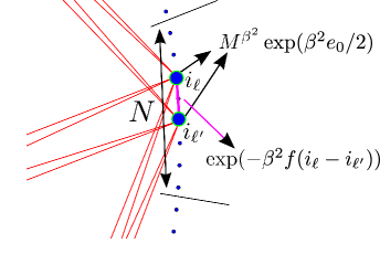
Figure 2.12: An illustration of the 1RSB Ansatz. The circular model is divided into $M/N=16$ blocks. The $n=8$ replicas partitioned into groups of size $m=2$. The right figure zooms into the block occupied by one group. The lines indicate the Wick contractions. The red (IR) ones should be calculated using eq. (2.146) and the violet (UV) ones should be calculated with eq. (2.147). See also Figure 2.8.

In this section we explain that the above 1RSB Ansatz implies the freezing scenario in logREM. For the sake of concreteness, let us still take the circular model of $1/f$-noise as example, see section 2.2.2 for definition. The basic idea of replica grouping is depicted in Figure 2.12. We divide the system into blocks of $N$ sites, where $N$ is any intermediate scale such that both $N$ and $M/N$ go to $+\infty$ in the thermodynamic ($M\to\infty$) limit. Each block will be labelled by their position $\theta\in[0,2\pi)$, or $z=e^{\mathbf{i}\theta}$, since all the lattice points in a same block will converge to the same continuum position as $M/N\to\infty$; positions inside a block will be labelled $1,\dots,N$; in other words, we have a one-to-one correspondence $j(\theta,i)$ between the “global position” $j$ and the hierarchical one $(\theta,i)$.

Now, in the replicated partition function

$$\sum_{j_{1},\dots,j_{n}}\overline{\exp\left(-\beta\sum_{a=1}^{n}V_{j_{a}}\right)}\,,$$

the $n$ replicas form $n/m$ groups of size $m$; when $n$ is continued to complex values we will have $m=\min(1,1/\beta)$ by eq. (2.142). Each group will occupy a block $\theta_{1},\dots,\theta_{n/m}$, while distinct groups will be separated by system-size scale distances. This justifies that the sum over group positions can be replaced by continuum integral in the $M\to\infty$ limit. In addition to that, we need to sum over the “micro-positions” of the replicas their respective blocks. At last, one should not forget the combinatorial factor ($C_{n,m}$ below, see eq. (2.109)) corresponding to assigning the $n$ replicas into $m$ (distinguishable) groups. In summary, the sum over replica positions is rewritten as follows:

$$\sum_{j_{1},\dots,j_{n}}[\dots]\longrightarrow C_{n,m}\left(\frac{M}{N}\right)^{\frac{n}{m}}\int_{0}^{2\pi}\prod_{g=1}^{n/m}\frac{\mathrm{d}\theta_{g}}{2\pi}\sum_{i_{1},\dots,i_{n}}[\dots]\,,\,$$ (2.144)

$$C_{n,m}=\frac{\Gamma(1+n)}{\Gamma(1+m)^{n/m}\Gamma(1+n/m)}\,,\,$$ (2.145)

where $[\dots]$ denotes the disorder–averaged Boltzmann weights, which, by Wick theorem, is a product of “contractions” $\exp\left(\beta^{2}\overline{V_{j_{a}}V_{j_{b}}}\right),a,b=1,\dots,n$. We will also split them into two types, according to whether $a,b$ are in the same group or not. If they are not, we should use the IR limit of the $1/f$-noise circular model (see eq. (2.93)):

$$\overline{V_{j_{a}}V_{j_{b}}}\longrightarrow 2\ln\left|z_{g(a)}-z_{g(b)}\right|\,,$$ (2.146)

where $g(a)$ is the group to which $a$ belongs. When $a,b$ are in same group, we use the UV data (see eq. (2.94) and (2.2.2)):

$$\overline{V_{j_{a}}V_{j_{b}}}\longrightarrow 2\ln M+e_{0}-f(\left|i_{a}-i_{b}\right|)\,.$$ (2.147)

Collecting the equations eq. (2.144) through (2.147), we have the following:

$$\overline{\mathcal{Z}^{n}}\,\rightarrow\,M^{\frac{n}{m}(\beta^{2}m^{2}+1)}C_{n,m}\,\overline{Z_{m\beta}^{n/m}}\,E_{m,\beta}^{\frac{n}{m}}$$ (2.148)

$$\overline{Z^{k}_{b}}=\int_{0}^{2\pi}\prod_{g=1}^{k}\left[\frac{\mathrm{d}\theta_{g}}{2\pi}\right]\prod_{g<g^{\prime}}\left|e^{\mathbf{i}\theta_{g}}-e^{\mathbf{i}\theta_{g^{\prime}}}\right|^{-b^{2}}=\frac{\Gamma(1-kb^{2})}{\Gamma(1-b^{2})^{k}}$$ (2.149)

$$E_{m,\beta}=e^{\beta^{2}m^{2}e_{0}/2}\frac{1}{N}\sum_{i_{1},\dots,i_{m}=1}^{N}\prod_{l,l^{\prime}=1}^{m}\exp(-\beta^{2}f(i_{l}-i_{l^{\prime}}))\,.$$ (2.150)

Here, $E_{m,\beta}$ gathers the sum over inter-block positions and the intra–group contractions (using eq. (2.147)); while $\overline{Z^{k}_{b}}$ is the Dyson integral (see eq. (2.69)) that results from the IR limit data eq. (2.146) and continuum integrals in eq. (2.144). It is continued to generic $k$ and $b$ Note that the Dyson integral appears in eq. (2.148) with “renormalized” temperature and number of charge numbers $b=\beta m,k=n/m$, as a result of grouping of replicas. Now let us discuss the result in the two phases.

High temperature phase

In the $\beta<1$ phase, by (2.142), $m=1$, so $b=\beta,k=n/m=n$, and $C_{n,m}=1$. $E_{m,\beta}$ becomes quite easy to evaluate: $E_{1,\beta}=e^{\beta^{2}e_{0}/2}$. With all that, eq. (2.148) implies

$$\overline{\mathcal{Z}^{n}}= \overline{Z_{\beta}^{n}}\left(M^{\beta^{2}+1}e^{\beta^{2}e_{0}/2}\right)^{n}\Leftrightarrow\overline{\exp(t\mathcal{F})}=e^{tF_{0}}\Gamma(1+t\beta)$$ (2.151)

where the second equation is obtained with the change of variable $n=-t/\beta$ (since $\mathcal{F}=-\beta^{-1}\ln\mathcal{Z}$), and the first moment shift part of the free energy is:

$$F_{0}= -\left(\beta+\beta^{-1}\right)\ln M-\beta e_{0}/2+\beta^{-1}\ln\Gamma(1-\beta^{2})\,,\beta<1\,.$$ (2.152)

The last factor comes from the denominator $\Gamma(1-\beta^{2})^{n}$ in the Dyson integral eq. (2.149). Equation (2.151) means the re-shifted free energy $f=\mathcal{F}-F$ satisfies $\overline{\exp(tf)}=\Gamma(1+t\beta)$, i.e., it has the same distribution as $-\beta$ times a Gumbel variable. This determines completely the free energy distribution in the $M\to\infty$ limit. The result confirms what we have found in section 2.1.3, eq. (2.70a).

Low temperature phase: freezing of distribution

The $\beta>1$ case is more interesting because it is directly related to the freezing scenario; it also involves a few subtleties that are not completely understood.

Let us begin with the combinatorial factor $C_{n,m}$. By analogy to what we have seen in the REM, when $n$ and $m$ become non-integer, they should be “continued” by applying the rule eq. (2.114):

$$C_{n,m}=\frac{\Gamma(1+n)}{\Gamma(1+m)^{\frac{n}{m}}\Gamma\left(1-\frac{n}{m}\right)}\leadsto\frac{\Gamma(1-m)^{\frac{n}{m}}\Gamma\left(1+\frac{n}{m}\right)}{\Gamma(1-n)}\,.$$ (2.153)

This manipulation has no satisfactory justification to the best of our knowledge. Carrying it out in eq. (2.148), and recalling that in this phase, eq. (2.142) implies $m=1/\beta$, so $b=1,n/m=n\beta$, we obtain:

$$\overline{\mathcal{Z}^{n}} =M^{2n}\frac{\Gamma(1-m)^{\frac{n}{m}}\Gamma\left(1+\frac{n}{m}\right)}{\Gamma(1-n)}\left.\frac{\Gamma(1-n\beta)}{\Gamma(1-b^{2})^{n}}\right|_{b\to 1}E_{m,\beta}^{n\beta}$$ (2.154)

$$\Rightarrow\overline{\exp(t\mathcal{F})} =e^{tF_{0}}\frac{\Gamma(1+t)^{2}}{\Gamma(1+t/\beta)}$$ (2.155)

where the free energy shift is now formally

$$F_{0}=-2\ln M-\beta e_{0}/2+\beta^{-1}\Gamma(1-b^{2})|_{b\to 1}-\ln E_{1/\beta,\beta}\,.\,\beta>1\,,$$ (2.156)

which is a quite problematic expression. Ignoring it for the moment, let us relate immediately eq. (2.155) to the freezing scenario; indeed, that equation implies that, denoting $g$ a standard Gumbel random variable independent of $\mathcal{F}$, we have

$$\overline{\exp(t(\mathcal{F}-\beta^{-1}g))}=\overline{\exp(t\mathcal{F})}\Gamma(1+t/\beta)=e^{tF_{0}}\Gamma(1+t)^{2}\,,$$ (2.157)

i.e., up to a translation, the distribution of $\mathcal{F}-\beta^{-1}g$ maintains its $\beta=1$-form in the whole $\beta>1$-phase. By inverse Laplace transform eq. (2.11) (or eq. (2.13b)), this means $G_{\beta}(x)=\overline{\exp(-e^{\beta x}\mathcal{Z})}$ is also temperature-independent (up to a global shift) in the $\beta>1$ phase. In summary, by the 1RSB analysis, we recovered the freezing of the limit shape (eq. (2.64b)) that we took for granted in section 2.1.3 (see discussion around eq. (2.71)). Although we obtained this result by the RSB approach, we note that recent mathematical developments in multiplicative chaos and in discrete 2D GFF have led to rigorous proofs of analogous results in respective settings [93, 112].

At last, we shall comment on the term $E_{m,\beta}$. The alert Reader should have noticed that we have already analytically continued it to generic complex $m\in\mathbb{C}$, without indicating how this is possible from the definition eq. (2.150). We shall postpone this discussion to section 2.5, around eq. (2.230).

Log–correction and duality

In the BBM model, we explained the $\ln\ln M$ corrections by an argument based on the KPP equation (eq. (2.56)); for logREM defined on the Euclidean plane, these properties are part of the general prediction (eq. (2.64)) that was put forward in [11], which showed that $G_{\beta}(x)$ still satisfy approximately KPP equations (see discussion after eq. (2.64)). To reconcile the current 1RSB formalism and the KPP approach is the subject of ongoing joint investigation. Therefore, we cannot present a general and systematic derivation of these universal features in the RSB framework. In fact, a major drawback of the RSB methods in general is the difficulty to access sub–leading corrections: even for the REM and DPCT/BBM, such progress is made only recently [103, 104] and relies on replica–free methods, as in section 2.1.1.

However, as the list of exactly solved logREM extends, a pattern has emerged for the analytically continued integrals. Let us take again the example of the circular model; by Dyson integral eq. (2.149), we have

$$\overline{Z_{b}^{-t/b}}\Gamma(1+t/b)=\Gamma(1-b^{2})^{\frac{t}{b}}\times\Gamma(1+tb)\Gamma(1+t/b)\,.$$ (2.158)

Notice two features of the right hand side: i the first factor vanishes as $\propto(1-b)^{t}$ as $b\to 1$. ii the remainder is invariant under the $b\leftrightarrow b^{-1}$ duality transform. In [90, 113], feature i was related to the $\frac{3}{2}\ln\ln M$ in the $\beta>1$ phase, especially in the ro–temperature limit. We shall not review the argument, which requires a formalism (counting statistics) not introduced in this thesis. Nevertheless, we can already see that in eq. (2.155) and (2.156), feature i induces a diverging ($\to+\infty$) shift of the free energy with respect to $-2\ln M$. The non–trivial task (undertaken in op. cit.) is to associate this divergence to si–dependent $\ln\ln M$ corrections.

The feature ii, known as the “duality invariance”, has been associated to freezing by the freezing–duality conjecture, see discussion around eq. (2.72). What can be said about this conjecture in the 1RSB framework? Although the latter does not demonstrate this conjecture, some instructive observation can be made. Indeed, recall that eq. (2.158) enters into the freezing distribution, that of $y:=\exp(\mathcal{F}-g-F_{0}$, eq. (2.157), with $b=\beta m=1$, since $m=1/\beta$ in the $\beta>1$ phase. Now, recall that in the RSB formalism, $m$ is a parameter that was optimized, in the full RSB analysis, see eq. (2.136) and (2.137). There, only the leading behaviour of free energy was considered. In [6] we argued that the same $m$ is optimal (stationary) also for all the higher cumulants of the free energy. Indeed, if we regard $m$ as a free parameter in eq. (2.155), we would have

$$\overline{\exp(t(\mathcal{F}-F_{0})}=\Gamma(1+t/\beta)^{-1}\Gamma(1+tm\beta)\Gamma(1+t/(m\beta))\,,\,$$

so by duality invariance,

$$\left[\frac{\partial}{\partial m}\overline{\exp(t(\mathcal{F}-F_{0}))}\right]_{m=1/\beta}=0\quad\Rightarrow\quad\left.\frac{\partial}{\partial m}\overline{\mathcal{F}^{k}}^{c}\right|_{m=1/\beta}=0\,,\,k=2,3,\dots\,.$$ (2.159)

Heuristically, this means that, just as its extensive free energy, which corresponds to the selected velocity in KPP equation, the whole limit distribution of the free energy is also “selected”. Turning this intuition into precise predictions is a goal of ongoing research.

To conclude this section, we emphasize that the quantitative understanding of the minimum distribution of the circular model (and other logREM on Euclidean spaces) is not complete: the first moment is still not determined to an $O(1)$ precision.

2.3.4 Pre–freezing and binding transition

The freezing transition is the only critical behaviour when we consider the extensive free energy in standard logREM such as the circular model. Other transitions can occur when more involved observables are considered, and/or in enriched logREM. Two examples have already appeared in the context of multi–fractality (section 2.1.4). In this section, we will first review the pre–freezing transition, and then study the binding transition, which is necessary for constructing the relation to Liouville field theory in section 2.6.

Pre–freezing transition

In this work, we use the term pre–freezing transition to refer to the transition associated with the divergence of the continuum Coulomb gas integrals; so, the term has a different meaning than that of the work [89], in which the same term refers to the termination point transition in this thesis; see section 2.1.4 for a clarification.

Recall that the Dyson integral eq. (2.69),

$$\overline{Z^{n}}=\int_{0}^{2\pi}\prod_{a=1}^{n}\frac{\mathrm{d}\theta_{a}}{2\pi}\prod_{1\leq a<b\leq n}\left|z_{a}-z_{b}\right|^{-2\beta^{2}}\,.$$

is convergent if and only if

$$n\beta^{2}<1\,.$$ (2.160)

Indeed, this condition applies to general Coulomb gas integrals representing continuum replica averages of logREM, because the divergence comes from configurations where the replicas $\theta_{1},\dots,\theta_{n}$ are very close. The power–counting of the integrand (and measure) is

$$\mathrm{d}(\theta_{2}-\theta_{1})\dots\mathrm{d}(\theta_{n}-\theta_{1})\prod_{a<b}\left|\theta_{a}-\theta_{b}\right|^{-2\beta^{2}}\sim[\theta]^{n-1-\beta^{2}n(n-1)}=[\theta]^{(n-1)(1-n\beta^{2})}\,,$$

where we note that due to translation invariance, the measure’s contribution is $[\theta]^{n-1}$. The integral diverges if the exponent $(n-1)(1-n\beta^{2})>0$, which is eq. (2.160). Note that when $\beta\geq 1$, eq. (2.160) means $n<\beta^{-2}\leq 1$. So the freezing transition $\beta=1$ happens when $\overline{Z^{n\to 1}}$ ceases to exist. When $n>1$, eq. (2.160) gives a higher pre–freezing critical temperature $\beta_{c,n}=n^{-1/2}<1$: they can be heuristically considered as precursors of the freezing temperature $\beta_{c}=\beta_{c,1}$. However, what is the physical interpretation of pre–freezing? The answer, given in [14], is that it corresponds to a transition in the negative large deviation of the free energy $\mathcal{F}$, and we review their treatment here, restricting to the $\beta<1$ phase.

For this, we recall from eq. (2.151) the Laplace transform of the shifted free energy

$$\overline{\exp(tf)}=\Gamma(1+t\beta)=\frac{1}{1+t\beta}+\dots\,,\,f=\mathcal{F}+(\beta+1/\beta)\ln M+O(1)\,,$$

where $\dots$ denotes poles at $t=-2/\beta,-3/\beta$. By inverse Fourier transform, this corresponds to the exponential tail

$$P(f)=e^{f/\beta}+O(e^{2f/\beta})\,,\,f_{*}\ll f\ll 0\,.$$ (2.161)

The crucial point is that eq. (2.151) is not valid for $t<-1/\beta$, so eq. (2.161) will cross over to some other distribution when $f<f_{*}$ for some $f_{*}$. To determine that distribution and $f_{*}$, we need to compute $\overline{\exp(tf)}$ for $t<-\beta^{-1}$, or $\overline{\mathcal{Z}^{n}}$ for $n=-t/\beta>\beta{-2}$: this is exactly the opposite condition of eq. (2.160). As argued in [76], this is a new phase with another type of RSB : all the $n$ replicas are in the same block; that is, we plug $m=n$ into (2.148), so the Coulomb gas integral eq. (2.149) becomes trivial, and we obtain:

$$\overline{\mathcal{Z}^{n}}=M^{\beta^{2}n^{2}+1}E_{n,\beta}\,,\,n>1/\beta^{2}$$ (2.162)

$$\Rightarrow\quad \overline{\exp(t\mathcal{F})}=M^{t^{2}+1}E_{-t/\beta,\beta}\,,\,t<-1/\beta\,.$$ (2.163)

By inverse Fourier transform this gives a Gaussian of variance $2\ln M$

$$P(f)=\frac{M}{\sqrt{4\pi\ln M}}\exp\left(-\frac{(f+F)^{2}}{4\ln M}\right)\,,\,f<f_{*}\,.$$ (2.164)

where $E_{-t/\beta,\beta}$ gives an $O(1)$ convolution which we have omitted. Note that $P(f)$ is not a normalized distribution on the whole real line: $\int_{\mathbb{R}}P(f)\mathrm{d}f=M$, so it can be only valid for $f<f_{*}$. To determine $f_{*}$ (up to order $\ln M$), we match eq. (2.164) with eq. (2.161):

$$f_{*}/\beta\approx\ln M-\frac{(f_{*}+F)^{2}}{4\ln M}\Rightarrow f_{*}=-(\beta^{-1}-\beta)\ln M+O(\ln\ln M)\,.$$ (2.165)

In summary, the exponential tail of eq. (2.161) crosses over to a Gaussian tail in the large deviation regime of atypically small free energy $\mathcal{F}=-(\beta+1/\beta)\ln M+f_{*}=-2\beta^{-1}\ln M$. By eq. (2.165), (2.164) and (2.161), we compute the (negative) large deviation function of free energy:

$$\mathcal{L}(x)\stackrel{{\scriptstyle\text{def.}}}{{=}}\frac{-1}{\ln M}\ln\overline{\left(\frac{\mathcal{F}}{\ln M}-x\right)}\stackrel{{\scriptstyle\beta<1}}{{=}}\begin{dcases}-x/\beta-1-1/\beta^{2}\,,&-2\beta^{-1}<x<-(\beta+\beta^{-1})\,,\\ x^{2}/4-1\,,&x<-2\beta^{-1}\,.\end{dcases}$$ (2.166)

The transition at $-2\beta^{-1}$ is the physical interpretation of the pre–freezing transition. Note that although the 1RSB solution jumps from $m=1$ (high temperature phase) to $m=n$ (pre–freezing phase) at the transition, $\mathcal{L}(x)$ has continuous derivative at the transition. Approaching the freezing temperature $\beta\to 1_{-}$, the pre–freezing point $-2/\beta\to-2$ comes close to the typical free energy density $-(\beta+\beta^{-1})$. So the same analysis in the $\beta>1$ phase requires carefully accounting for the $\ln\ln M$–order corrections.

Binding transition

Let us consider a concrete model that displays the binding transition, the Morris circular model (another example is the interval model, considered in [76]). Recall that, the potential of the circular model can be seen as restricting the 2D GFF $\phi$ (eq. (2.59)) to the unit circle. In this respect, the random potential of the Morris circular model can be seen as $\phi(z)+2\alpha\ln\left|z-1\right|$. That is, we add a deterministic part of the potential which has a logarithmic singularity, here at $z=1$. To define it properly on a lattice, let $C_{jk},j,k=1,\dots,M$ be the covariance matrix of the circular model (defined by eq. (2.91) and (2.92a)). Then, that of the Morris circular model is defined by:

$$\overline{V_{j}}=-\alpha C_{j1}\,,\,\overline{V_{j}V_{k}}^{c}=C_{jk}\,.$$ (2.167)

Here we assume that the lattice points are given by $z_{j,M}=e^{2\pi j/M}$. Then by eq. (2.93), it is clear that $\overline{V_{j}}\to 2\alpha\ln\left|z-1\right|$ provided $z_{j,M}\to z\neq 1$ as $M\to\infty$: the mean values in eq. (2.167) reproduce the continuum potential $2\alpha\ln\left|z-1\right|$. On the other hand, its divergence at $z=1$ is regularized by $\overline{V_{1}}=-2\alpha\ln M+O(1)$.

The binding transition happens when $a$ is large enough that the thermal particle is trapped at $z=1$. The easiest way to establish the phase diagram (in the plane of $(\beta,\alpha)$) is the following argument (already present in [11], Appendix D, see also [7]). The free energy of the particle sitting at $z=1$ is $F_{1}=V_{1}=-\alpha\ln M+O(\sqrt{\ln M})$; on the other hand, the free energy staying away from $z=1$ is simply that of the circular model, $F_{0}\sim Q\ln M+O(1)$, see eq. (2.72). Then, the criterion of no–binding is $F_{0}\ll F_{1}$ as $\ln M\to\infty$, which gives

$$\alpha<Q/2\,,\,Q=\begin{cases}\beta^{-1}+\beta\,,\,&\beta<1\,,\\ 2\,,&\beta\geq 1\,.\end{cases}$$ (2.168)

Therefore, the Morris circular model has three phases, the high temperature phase $\beta<1,\alpha<\beta^{-1}+\beta$, and frozen phase $\beta>1,\alpha<2$, and the bound phase $\alpha>Q/2$ with $Q$ defined above. The phase diagram is drawn in Figure 2.13 (Left panel).

Figure 2.13: (Left) The phase diagram of logREM with a logarithmic potential, such as the Morris circular model. The blue vertical line is the freezing transition, while the other (near horizontal) curve is the binding transition line, $a=Q/2$, see eq. (2.168). (Right) The minimum variance of Morris circular model as a function of the log of system size, compared to $2\ln M+c$ ($\alpha=1.5$, bound phase), $\ln M+c^{\prime}$ ($\alpha=1$, zero temperature critical) and $c^{\prime\prime}$ ($\alpha=.5$, frozen phase).

In the high temperature and frozen phase, the free energy distribution of the Morris circular model can be studied using the same method as applied to the interval model [76]; in particular, we still have $\mathcal{F}=-Q\ln M+\eta\ln\ln M+O(1)$. In the bound phase, the thermal particle is trapped at $j=1$, so its free energy $\mathcal{F}\approx V_{1}$, thus we predict

$$\overline{\mathcal{F}}=-\alpha\ln M+O(1)\,,\,\overline{\mathcal{F}^{2}}^{c}=2\ln M+O(1)\,,\alpha>1\,.$$ (2.169)

So, the variance of the free energy is not $O(1)$ but is extensive. A numerical test (in the zero temperature) of this latter prediction is given in Figure 2.13 (Right panel). We observe also that $\overline{\mathcal{F}^{2}}^{c}\approx\ln M+O(1)$ in at the (zero–temperature) binding transition $\beta=\infty,\alpha=1$.

The discrete definition eq. (2.167), and the no–binding condition eq. (2.168) are not specific to the Morris circular model, but apply to any logREM. In the $d$-dimensional Euclidean space, the covariance matrix has a logarithmic decay given by eq. (2.89), so the mean value is

$$\overline{V_{j}}=U(\mathbf{x}_{j})\,,\,U(\mathbf{x})\sim 2d\alpha\ln\left|\mathbf{x}-\mathbf{x_{1}}\right|\,,$$ (2.170)

where $(\mathbf{x_{j}})_{j=1}^{M}$ is the lattice of the logREM. Equation (2.168) gives the condition that the thermal particle is not bound near $\mathbf{x_{1}}$. The consideration generalize naturally to potentials with several logarithmic singularities: they will be used when studying the mapping of logREM to Liouville field theory in section 2.6.

2.4 Application of Jack polynomials

This section will review applications of Jack polynomials to the circular model of $1/f$-noise and its variants, based on results reported in [3] (section 2.4.2), and in [4] (sections 2.4.3 and 2.4.4). Although applications of Jack polynomials to logREM are rather recent (in [80] and op.cit.), the idea is very natural and straightforward. Indeed, the replica trick applied to logREM produces systematically Coulomb gas integrals of the following form:

$$\int\mathrm{d}z_{1}\dots\int\mathrm{d}z_{n}\prod_{a<b}\left|z_{a}-z_{b}\right|^{-2\beta^{2}}f(z_{1},\dots,z_{n})\,,\,$$ (2.171)

where $f(z_{1},\dots,z_{n})$ is a symmetric function of $z_{1},\dots,z_{n}$. The Dyson integral eq. (2.69) is a simplest case where $f=1$. In general, such integrals are difficult to evaluate into a form that can then be analytically continued (to $n$ non–integer!). Yet, this task becomes possible when $f$ is a Jack polynomial (or product of two of them). So the strategy will be to use the Jack polynomials as a basis to expand $f$, and then integrate term by term. For this, we need some mathematical results, which we review in the following section.

2.4.1 Jack polynomials

Jack polynomials [114] are a family of symmetric polynomials. The latter is a classical subject in mathematics, related to representation theory of semi–simple Lie groups and permutation groups, as well as to combinatorics; see [115], last chapter for a comprehensive introduction and extended references. The classical (19th century) theory is focused on the Schur polynomials. In the 20-th century, a few other families of symmetric polynomials have been considered as non-trivial generalizations of the Schur class, e.g., the Jack polynomials and the Macdonald polynomials. A classical treatment is MacDonald’s book [116], which will be our main reference and set the conventions.

The last two polynomials have important physical applications. The Macdonald polynomials play an important rôle in the development of quantum integrable system related to the Kardar–Parisi–Zhang (KPZ)equation in $(1+1)$-dimension [117] (it is impossible to give a fair review of this fast growing field here, however, see [118] for introduction and [119] for summary). The Jack polynomials can be obtained as a degenerate case of Macdonald polynomials, but have arguably wider applications. They are closely related to eigen-functions of the Calegero-Sutheland quantum integrable system (see [120, 121] for introduction), and thus related to fractional statistics (see [122] for introduction). More recent developments include important applications in fractional quantum Hall effects [123], and in conformal field theory with extra symmetry [124, 125, 126].

Definition

The Jack polynomials $P_{\lambda}^{(\alpha)}(\underline{z}),Q_{\lambda}^{(\alpha)}(\underline{z})$ are symmetric polynomials in the set of $n$ variables $\underline{z}=(z_{1},\dots,z_{n})$, i.e., $P_{\lambda}^{(\alpha)}(z_{1},\dots,z_{n})=P_{\lambda}^{(\alpha)}(z_{\sigma(1)},\dots,z_{\sigma(n)})$ for any permutation $\sigma$ of $n$ numbers. They depend on a complex parameter $\alpha$ and are indexed by an integer partition $\lambda$. This is an important combinatorial notion for the theory of symmetric polynomials, so we briefly review it here (for a detailed treatment, see the first section of [116]).

An integer partition $\lambda$ can be defined as a finite sequence of decreasing positive integers $\lambda=(\lambda_{0}\geq\lambda_{1}\dots\lambda_{\ell(\lambda)}>0)$, where $\ell(\lambda)$ is called its length, while its size is defined as $\left|\lambda\right|=\lambda_{1}+\dots+\lambda_{\ell(\lambda)}$. It is clear that integer partitions of size $n$ and length $\ell$ are in one–to–one correspondence with the ways of decomposing $n$ as sum of $\ell$ non-ro integers, if re-ordering is not considered to give a different sum (this is the reason of the name). A common representation of the integer partitions is the Young diagram. The Young diagram of a partition $\lambda$ is the set

$$\lambda\mapsto\{(x,y)\in\mathbb{N}^{2}|x=0,1\dots,\lambda_{y}-1\,,\,y=0,1,\dots,\ell(\lambda)-1\}$$

of integer pairs. In the following, we will identify $\lambda$ with the right hand side. Graphically, each pair is drawn as a box in the 2d plane. To illustrate, we enumerate all the partitions with size $\leq 3$ in Table 2.14. Note that the empty sequence $\emptyset$ is also considered as a partition of si/length $0$.

The Young diagram representation make it easy to define the transpose of a partition, $\lambda^{t}$, as obtained by applying the $(x,y)\mapsto(y,x)$ transform. In terms of the sequence, it is not hard to see that $\lambda^{t}_{j}=\left|i:\lambda_{i}\geq j\right|$. For instance, when $\lambda=(3)$, $\lambda^{t}=(1,1,1)$.

Young diagram	$\lambda$	$\ell(\lambda)$	$\left|\lambda\right|$
	$()=\emptyset$	$0$	$0$
	$(1)=\square$	$1$	$1$
	$(2)$	$1$	$2$
	$(1,1)$	$2$	$2$
	$(3)$	$1$	$3$
	$(2,1)$	$2$	$3$
	$(1,1,1)$	$3$	$3$

Figure 2.14: Enumeration of all the partitions of size $\leq 3$.

Main properties

The explicit form of Jack polynomials are not so important for our applications as their properties:

1. $P_{\lambda}^{(\alpha)}(\underline{z})$ and $Q_{\lambda}^{(\alpha)}(\underline{z})$ are related by a factor

   $$Q_{\lambda}^{(\alpha)}(\underline{z})=J_{\lambda}^{(\alpha)}P_{\lambda}^{(\alpha)}(\underline{z})\,.$$ (2.172)

   The explicit form of $J_{\lambda}^{(\alpha)}$ is not important here.

2. $P_{\lambda}^{(\alpha)}(\underline{z})$ is defined for $\underline{z}=(z_{1},\dots,z_{n})$ with different numbers variables $n$. They are related by

   $$P_{\lambda}^{(\alpha)}(z_{1},\dots,z_{n-1})=P_{\lambda}^{(\alpha)}(z_{1},\dots,z_{n-1},z_{n}=0)\,,$$ (2.173)

   and the same is true for $Q_{\lambda}^{(\alpha)}$. This fact justifies omitting the dependence on $n$ in the notations. In fact, it is sometimes useful to define Jack polynomials as symmetric polynomials of an infinite sequence of variables $z_{1},\dots,z_{n},\dots$, and obtain the finite-$n$ versions by setting $z_{n+1}=z_{n+2}=\dots=0$.

3. Both $P_{\lambda}^{(\alpha)}(\underline{z})$ and $Q_{\lambda}^{(\alpha)}(\underline{z})$ are homogeneous polynomials of order $\left|\lambda\right|$, i.e.,

   $$(P_{\lambda}^{(\alpha)}(az_{1},\dots,az_{n})=a^{\left|\lambda\right|}P_{\lambda}^{(\alpha)}(z_{1},\dots,z_{n})\,,\,$$ (2.174)

   and the same is true for $Q_{\lambda}^{(\alpha)}$.

4. Cauchy identity:

   $$\prod_{a=1}^{n}\prod_{b=1}^{m}(1-z_{a}w_{b})^{-1/\alpha}=\sum_{\lambda}P_{\lambda}^{(\alpha)}(\underline{z})Q_{\lambda}^{(\alpha)}(\underline{w})\,,$$ (2.175)

   where $\underline{w}=(w_{1},\dots,w_{m})$. Note that the sum in the right hand side is over all the partitions, with no restriction of size, so it is an infinite series. Technically, the identity holds in a sense of formal power series (i.e., matching of all coefficients).

5. Orthogonality with respect to integration on the unit circle:

   $$\int_{0}^{2\pi}\prod_{a=1}^{n}\frac{\mathrm{d}\theta_{a}}{2\pi}\prod_{a<b}\left|z_{a}-z_{b}\right|^{\frac{2}{\alpha}}P_{\lambda}^{(\alpha)}(\underline{z})Q_{\mu}^{(\alpha)}(\underline{z^{*}})=\delta_{\lambda\mu}p_{n}^{\lambda}(\alpha)c_{n}(\alpha)\,,$$ (2.176a)

   where $$\delta_{\lambda\mu}=1 \lambda=\mu 0$$ if and only if are the same partition, but otherwise,

   $$c_{n}(\alpha)=\int_{0}^{2\pi}\prod_{a=1}^{n}\frac{\mathrm{d}\theta_{a}}{2\pi}\prod_{a<b}\left|z_{a}-z_{b}\right|^{\frac{2}{\alpha}}=\frac{\Gamma(1+n/\alpha)}{\Gamma(1+1/\alpha)^{n}}\,,$$ (2.176b)

   is the Dyson integral (eq. (2.69)), and finally

   $$p_{n}^{\lambda}(\alpha)=\prod_{(x,y)\in\lambda}\frac{\alpha x+n-y}{\alpha(x+1)+n-(y+1)}\,,$$ (2.176c)

   is a product over all the boxes in the Young diagram of $$\lambda n=1,2,3,\dots$$. Note that the orthogonality relation depends explicitly on the number of variables .

Among the above properties, the last two (Cauchy identity and orthogonality) are the most important and will be crucial for calculating the Coulomb gas integrals in the next two sections. Remark that orthogonality property makes the Jack polynomials the multi–variable analogue of the exponential/trigonometric functions $e^{\mathbf{i}k\theta},k=0,\pm 1,\pm 2,\dots$ with respect to the integral measure $(2\pi)^{-1}\int_{0}^{2\pi}\mathrm{d}\theta[\dots]$ on the unit circle. Now, another property of the trigonometric functions is that they form a complete basis (of the Hilbert space of square–integrable functions on the unit circle). Similarly, the Jack polynomials form a complete basis of the symmetric functions (defined on the torus $\left\{(z_{1},\dots,z_{n}):\left|z_{i}\right|=1\right\}$). Although we will not need this property explicitly in sections 2.4.2 through 2.4.4, we believe that it will be important for future applications, as we discuss in section 2.7.

2.4.2 Dirichlet circular model

The Dirichlet circular model was formally introduced in section 2.2.2, see eq. (2.92b), as a deformation of the standard circular model with different a IR data , eq. (2.93). The motivation of studying this model (whose definition went back to [76]) was the following more ambitious questions, which are all still open: how can we extend the exact calculation of the free energy distribution of the circular and interval model to more general curves or 2d domains? Does the freezing–duality conjecture (see discussion around eq. (2.72)) in general? A more specific motivation (stressed in [3]) is the IR divergence of 2D GFF, see section 2.2.3 for more discussion. Indeed, 2D GFF must be defined on a finite geometry, i.e., a 2D sphere or a disk. However, the 2D Coulomb–gas integrals on these geometries are not exactly solved (this is a major open problem in mathematical physics, with applications in 2D one-component plasma [78] and in fractional Quantum Hall Effect, see [127, 128, 129] for recent developments). So we shall simplify the problem to considering the logREM obtained by restricting a finite-domain 2D GFF to a circle in that domain. The 2D GFF on the sphere will be discussed in more detail in section 2.6. As shown in [3], the circular model defined on a sphere is easily related to the standard one. So we will turn to the 2D GFF on a disk.

2D GFF on a disk

Figure 2.15: A sample of the 2D GFF in a unit disk with Dirichlet boundary condition, and its restriction on a centred circle. The latter defines the circular Dirichlet model, after removing the zero mode.

Consider a centred disk of radius $R>1$ in the complex plane, $\left\{z:\left|z\right|<R\right\}$. The 2D GFF with Dirichlet boundary condition is defined by the following Green function:

$$\overline{\phi(z)\phi(w)}=G_{R}(z,w)=-2\ln\left|\frac{z-w}{R-zw^{*}/R}\right|\,,\,\left|z\right|,\left|w\right|<R\,.$$ (2.177)

$G_{R}(z,w)$ satisfies the Laplace equation $\Delta_{z}G_{R}=0$ with the Dirichlet boundary condition $G_{R}(Re^{\mathbf{i}\theta},w)=0$ for any $\theta\in\mathbb{R}$ and $w\in\mathbb{C}$. Rewriting eq. (2.177) as follows,

$$G_{R}(z,w)=-2\ln\left|\frac{z-w}{1-qzw^{*}}\right|+2\ln R\,,\,q=R^{-2}\in(0,1)\,,$$ (2.178)

we can identify it with the Dirichlet circle case in eq. (2.93), if the term $2\ln R$ is discarded. So if we restrict the Dirichlet 2D GFF (eq. (2.177)) to the unit circle, we will obtain a 1D log-correlated potential which is that of the Dirichlet circular model plus a zero-mode, i.e., we may define $\phi(e^{\mathbf{i}\theta})=\varphi(e^{\mathbf{i}\theta})+\phi_{0}$, where $\phi_{0}$ is a centred Gaussian distribution of variance $2\ln R$ and is independent of $\varphi$, while the latter satisfies

$$\overline{\varphi(z)\varphi(w)}=-2\ln\left|\frac{z-w}{1-qzw^{*}}\right|\,,\,\left|z\right|=\left|w\right|=1\,.$$ (2.179)

The effect of the zero mode to the free energy distribution is trivial, so we will focus on eq. (2.179). Nevertheless, with respect to the discussions in section 2.2.3 (around eq. (2.103)), we remark that as $q\to 0$ ($R\to\infty$), the circular model in the Dirichlet disk with ro mode (i.e., defined by eq. (2.178)), is an IR divergent logREM, in the sense that its free energy is the convolution of a Gaussian of diverging variance ($2\ln R$) coming from the ro–mode, and a correction distribution, which is the free energy of the model with ro–mode removed, eq. (2.179). Here, the correction is a well–defined probability distribution (in contrast to the Gaussian model), thanks to the fact that eq. (2.179) is defined on a finite geometry.

We have seen in section 2.2.2 (eq. (2.92b)) how to define a discrete logREM whose IR data is eq. (2.179). Note that the limit $q\to 0$ gives back the original circular model corresponding to the infinite plane ($R\to\infty$). The Dirichlet circular model is also defined formally for $q\in[-1,0)$; a rather artificial physical interpretation exists in terms of anti-symmetrid 2D GFF on the sphere ([3], section 1).

Solution by Jack polynomials

Now let us sketch the solution of the Dirichlet circular model. The approach is identical to that of the circular model 2.1.3, which starts by considering the continuum partition function

$$Z=\int_{0}^{2\pi}\frac{\mathrm{d}\theta}{2\pi}\exp(-\varphi(e^{\mathbf{i}\theta}))\,$$

where $\varphi$ satisfies eq. (2.179), and its replicated averages $\overline{Z^{n}}$. Therefore The essential technical novelty consists in extending the Dyson integral eq. (2.69) to the following Coulomb gas integral,

$$\overline{Z^{n}}=\int_{0}^{2\pi}\prod_{a=1}^{n}\frac{\mathrm{d}\theta_{a}}{2\pi}\prod_{a<b}\left|\frac{z_{a}-z_{b}}{1-qz_{a}z_{b}^{*}}\right|^{-2\beta^{2}},\;z_{a}:=e^{\mathbf{i}\theta_{a}}\,.$$ (2.180)

This is where Jack polynomials become useful, if the Jack parameter is related to $\beta$ by $\alpha=-\beta^{-2}$. Indeed, we can use the Cauchy identity eq. (2.175) (and the homogeneity eq. (2.174)) to expand the denominator above

$$\prod_{a<b}\left|\frac{1}{1-qz_{a}z_{b}^{*}}\right|^{-2\beta^{2}}=(1-q)^{-n\beta^{2}}\sum_{\lambda}q^{|\lambda|}P_{\lambda}^{(\alpha)}(\underline{z})Q_{\lambda}^{(\alpha)}(\underline{z})\,,$$

and then integrate each term obtained by the orthogonality relation eq. (2.176). The end result is:

$$\overline{Z^{n}}=(1-q)^{-n\beta^{2}}\frac{\Gamma(1-n\beta^{2})}{\Gamma(1-\beta^{2})^{n}}\sum_{\lambda}q^{|\lambda|}\prod_{(x,y)\in\lambda}\frac{x+(y-n)\beta^{2}}{x+1+(y+1-n)\beta^{2}}\,.$$ (2.181)

Although it is not an closed form formula, it provides an analytical continuation to $n\in\mathbb{C}$ of the Coulomb gas integral eq. (2.180), generalizing the Dyson integral (which is retrieved at $q=0$). Therefore we have the free energy distribution in the $\beta<1$ phase:

$$\overline{\exp(tf)}=\Gamma(1+t\beta)\mathbf{s}(t,\beta,q)\,,\,\beta<1\,,\,$$ (2.182)

$$\mathbf{s}(t,\beta,q)=\sum_{\lambda}q^{|\lambda|}\prod_{(x,y)\in\lambda}\frac{x\beta+y\beta^{-1}+t}{(x+1)\beta+(y+1)\beta^{-1}+t}\,.$$ (2.183)

Here, $f$ is related to the free energy by a shift, which absorbed the factors $(1-q)^{-n\beta^{2}}\Gamma(1-\beta^{2})^{-n}$ in eq. (2.181).

Figure 2.16: Taken from [3]. Real and imaginary part of $\overline{\exp(\mathbf{i}tf)}=\overline{\cos(tf)}+\mathbf{i}\overline{\sin(tf)}$ with $t\in\mathbb{R}$. The data points are obtained from numerically simulations, while the curves are the prediction eq. (2.183). In this Figure, both the predicted and numerical distribution have been shifted so as to have vanishing mean value. However, we have checked that the mean value can be also predicted by taking into account the UV data, see eq. (2.152).

Equations (2.182) and (2.183) are already non–trivial and non–rigorous predictions that should be checked. In [3], two tests were provided. The first (appendix B therein) is a comparison with the analytic high temperature expansion. The second is against numerical simulations. For this we need to evaluate the infinite sum eq. (2.183) to a sufficient approximation. Fortunately, this can be efficiently done by a transfer matrix method, describe in Appendix A of [3]. The comparison with numerical simulation confirms the analytic continuation eq. (2.182), see Figure 2.16 for an example.

Given the solution in the $\beta<1$ phase, we can apply the freezing scenario, in particular the freezing of limit shape in eq. (2.64b) (which is by now a consequence of the RSB, see section 2.3.3) to the $\beta>1$ phase. In particular, the distribution of the (shifted) minimum, $y$, is given by the following (via Laplace transform),

$$\overline{\exp(ty)}=\Gamma(1+t)^{2}\mathbf{s}(t,1,q)\,.$$ (2.184)

The inverse Laplace transform can be done numerically, and some results are plotted in Figure 2.17. The minimum distribution depends non–trivially on $q$, yet most of the dependence can be absorbed in a rescaling; the variance of the minimum distribution decreases as $q\to 1$, which is expected given the interpretation $q=R^{-2}$: when $R\to 1$, the unit circle approaches the disk boundary where the GFF is zero by the Dirichlet boundary condition.

Remark that by eq. (2.183), $\mathbf{s}(t,\beta=1,q)$ have poles only at $t=-2,-3,\dots$, so the rightmost pole of $\overline{\exp(ty)}$ is at $t=-1$ and of order $2$. By inverse Fourier transform, this implies $P(y\rightarrow-\infty)\sim A|y|e^{-|y|}$ for any $q$. This is a confirmation of the universality of the left–tail, predicted for general logREM, see eq. (2.64c).

Figure 2.17: Taken from [3]. Left panel: Distribution of the shifted minimum of the Dirichlet circular model for various values of $q$. All the distributions are obtained by numerical inverse Fourier transform applied to eq. (2.184), whereas the infinite sum in the last equation is efficiently calculated using the methods of [3]. Right panel: Distribution of the shifted minimum, rescaled so as to have unity variance. The rescaled distributions have still a non–trivial, although weak, dependence on the parameter $q$.

Duality

An interesting feature of the solution eq. (2.182) and (2.183) is its duality. Indeed, it is not hard to see from eq. (2.183) that

$$\mathbf{s}(t,\beta^{-1},q)=\mathbf{s}(t,\beta,q)\,,$$ (2.185)

because the term corresponding to $\lambda$ is transformed by the change of variable $\beta\mapsto\beta^{-1}$ to that of $\lambda^{t}$, the transpose of $\lambda$ (see section 2.4.1). As a consequence, by eq. (2.182), $\overline{\exp(tf)\Gamma(1+t/\beta)}$ is also invariant under the change of variable $\beta\to\beta^{-1}$. Therefore, the Dirichlet circular model provides a non-trivial check of the freezing-duality conjecture (section 2.1.3).

Moreover, the duality invariance is satisfied not only for the whole infinite series $\mathbf{s}(t,\beta^{-1},q)$, but also for every pair of transpose partitions (and every partition that is its own transform). This offers infinite potential opportunities of checking the freezing-duality conjectures. However, a prerequisite is finding the corresponding physical observables. The next section makes a first step in this direction, by interpreting the term corresponding to the first non-trivial term (corresponding to $\lambda=(1)=\square$), in terms of the Edwards-Anderson order parameter.

2.4.3 Edwards-Anderson order parameter

In this section and the next one, we shall go back to the original circular model ($q=0$). Up to now, the only observable we have considered is the free energy distribution, related to extreme value statistics. What about the extreme position statistics, or, in finite temperature, Gibbs measure statistics? Because of rotational invariance, the disorder–averaged Gibbs measure is trivially uniform. No higher order correlation function of the Gibbs measure is exactly known for the circular model.

In this respect, the Edwards–Anderson (EA) order parameter is among the few exact results (besides the prediction of Liouville theory, see 2.6, and predictions of [80]) concerning the Gibbs measure/position of the circular model. Its name is motivated by seeing the position, $\exp(2\pi\mathbf{i}j/M)$ on the unit circle as a $O(1)$ (XY–model) spin. For a given disorder average, one defines its thermal average as

$$\left<\xi\right>=\frac{1}{\mathcal{Z}}\sum_{j=1}^{M}e^{-\beta V_{j}}\exp(2\pi\mathbf{i}j/M)\,,\,\mathcal{Z}=\sum_{j=1}^{M}e^{-\beta V_{j}}\,,$$ (2.186)

where $V_{j},j=1,\dots,M$ are the potential values of the circular model of size $M$. We define the disorder–averaged modulus square of the above as the EA order parameter of the circular model, following the original proposition [31].

In [4], the Edwards–Anderson parameter was exactly calculated to be the following:

$$\overline{\left|\langle\xi\rangle\right|^{2}}\stackrel{{\scriptstyle M\rightarrow\infty}}{{=}}\begin{dcases}\frac{\beta^{2}}{1+\beta^{2}}\,,&\beta\leq 1\,,\\ \frac{2\beta-1}{2\beta}\,,&\beta\geq 1\,.\end{dcases}$$ (2.187)

We can make two remarks. First, the EA parameter is non-zero at any finite temperature. More interestingly, the non-analyticity at the freezing transition $\beta=1$ is very non-trivial. There is no evident reason to rule out the $\beta<1$ expression as a solution in the $\beta>1$ phase: the difference seems only quantitative. Nevertheless, the prediction eq. (2.187) is very well confirmed by numerical simulation, see figure (2.18).

Figure 2.18: Taken from [6]. Numerical check of the Edwards–Anderson order parameter of the circular model. The full curve plots the prediction eq. (2.187); the dashed curves plots the $\beta<1$ expression continued into the $\beta>1$ phase. The points come from direct numerical simulation.

Now let us briefly review two derivations of eq. (2.187), that of [4], using freezing–duality conjecture, and that of [6] (Appendix B), using 1RSB.

Freezing–duality conjecture

As is usually the case, the two approaches are the same in the $\beta<1$ phase, where it suffices to work in the continuum, and use the standard replica trick. For this, we consider the following observable $(z_{a}=e^{\mathbf{i}\theta_{a}})$

$$\overline{Z^{n}\left<\xi\right>^{2}}=\int_{0}^{2\pi}\prod_{a=1}^{n}\frac{\mathrm{d}\theta_{a}}{2\pi}\prod_{a<b}\left|z_{a}-z_{b}\right|^{-2\beta^{2}}z_{1}z_{2}^{*}$$ (2.188)

We can calculate it by relating it to eq. (2.181). For this, we expand the latter as a power series in $q$, and takes out the $q^{1}$ term:

$$\int_{0}^{2\pi}\prod_{a<b}\left|z_{a}-z_{b}\right|^{-2\beta^{2}}\sum_{a,b=1}^{n}z_{a}z_{b}^{*}=\frac{\Gamma(1-n\beta^{2})}{\Gamma(1-\beta^{2})}\frac{n}{n-1+\alpha}\,,$$ (2.189)

where the right hand side correspond to the partition $\lambda=(1)=\square$. This above equation is related to eq. (2.188) by symmetrization. Combining them, and expressing in terms of free energy ($n=-t/\beta$), we have

$$\overline{e^{tF}\left(\beta-(t+\beta)\left|\langle\xi\rangle\right|^{2}\right)}\stackrel{{\scriptstyle\beta<1}}{{=}}\frac{\Gamma(1+t\beta)}{\Gamma(1-\beta^{2})^{-\frac{t}{\beta}}}\times\frac{1}{t+\beta+\beta^{-1}}\,.$$ (2.190)

Note that setting $t=0$ gives already the $\beta<1$ phase part of eq. (2.187).

Now, the last factor of eq. (2.190) is the term corresponding to $\lambda=\square=(1)$ in the infinite sum (2.183). The Young diagram is symmetric, so the term is a function of the dual variable $\beta+\beta^{-1}$. So it is reasonable to apply the freezing–duality conjecture to that term. The remaining term is equal to $\overline{e^{tF}}$ itself, of which we know the $\beta>1$ phase behaviour. Defining the shifted free energy $f=F-\beta^{-1}\ln\Gamma(1-\beta^{2})$, the product of $\overline{e^{tf}}=\Gamma(1+t\beta)$ with $\Gamma(1+t/\beta)$ is dual and freezes in the $\beta>1$ phase.

$$\Gamma(1+t/\beta)\overline{e^{tf}\left(\beta-(t+\beta)\left|\langle\xi\rangle\right|^{2}\right)}\stackrel{{\scriptstyle\beta>1}}{{=}}\Gamma(1+t)^{2}\frac{1}{t+2}\,.$$ (2.191)

Setting $t=0$ gives the $\beta>1$ phase part of eq. (2.187). Such a treatment of the EA order parameter is an example to be generalized to further terms. Doing this would provide infinite series of duality–invariant observables, indexed by (pairs of) partitions, and hopefully a clarification on the origin and generality of the duality invariance.

1RSB insight

The above application of the freezing–duality conjecture is quite tricky, although the result is confirmed very well by numerics. However, the $\beta>1$ phase behaviour of the EA order parameter can be much better understood by the 1RSB. A more detailed account can be found in [6], appendix B. Here, let us give a simple argument in terms of the overlap distribution.

For this, note that the EA order parameter can be expressed as the inner product of the position of two independent thermal particles in a circular model: $\overline{\left|\langle\xi\rangle\right|^{2}}=\overline{\langle\xi_{1}\rangle\langle\xi_{2}\rangle^{*}}$, where $\xi_{1}$ and $\xi_{2}$ are the position of the two independent thermal particles.

Now, recall from section 2.3.2, discussion around eq. (2.143) and (2.142), that the two thermal particles have either overlap $\mathsf{q}=1$ or $\mathsf{q}=0$. The probability of $\mathsf{q}=1$ is $\beta^{-1}$ in the $\beta>1$ phase; by definition, when the overlap is $1$, the two particles are at the same continuum position, so $\overline{\left<\xi\right>\left<\xi^{*}\right>}\stackrel{{\scriptstyle\mathsf{q}=1}}{{=}}1$. The alternative conditional average can be obtained at the critical temperature, at which the overlap is always $0$: $\overline{\left<\xi\right>\left<\xi^{*}\right>}\stackrel{{\scriptstyle\mathsf{q}=0}}{{=}}\overline{\left<\xi\right>\left<\xi^{*}\right>}_{\beta=1}$. Adding the two possibilities, we obtain

$$\overline{\left|\langle\xi\rangle\right|^{2}}_{\beta>1}=1-\beta^{-1}\left(1-\overline{\left|\langle\xi\rangle\right|^{2}}_{\beta=1}\right)\,.$$ (2.192)

We can check that this formula correctly reproduces the result eq. (2.187). Moreover, the 1RSB reasoning reveals that $\overline{\left|\langle\xi\rangle\right|^{2}}_{\beta>1}$ is linear in the $\beta^{-1}$ in the $\beta>1$ phase; since it must be equal to $1$ at zero temperature, its value at $\beta=1$ suffices to determine completely its glassy phase behaviour.

2.4.4 Minimum and maximum

Another Jack polynomial application to the circular model is the joint min–max distribution. The treatment is quite similar to the Dirichlet circular model and was reported in considerable detail in [4]; so we will sketch the approach and some main results below. Before that let us give a few motivations of the question in a more general context (following [4]):

• The joint min–max distribution contains the distribution of the min–max difference. This quantity is more accessible to experiments, since it is the extremal width of the interface (log–correlated interfaces are studied experimentally [130, 131]), whereas the to define minimum value itself, one need a reference point.

• Properties of opposite extrema are related to the diffusion dynamics of an over-damped Langevin particle in the 1d potential. In particular, the max–min difference is the barrier that the particle should surmount to explore the whole system, and is thus related to Arrhenius passage times and to the diffusion coefficient in the periodic potential [132, 133, 134]. In the log–correlated 1D case, the freezing transition of logREM’s manifests itself also in the dynamical exponents [135].

• Since the opposite extrema are far apart in space and in value, they are often assumed to the independent. As shall see below, this is a good approximation, but a min–max correlation of order unity persists in the thermodynamic limit, and we will exactly predict (and test) it for the circular model.

Now let us review the technical part. In order to access the maximum (and minimum) from a thermodynamic approach as a zero temperature limit, one should simply consider a negative (and positive) temperatures. So, let us define the continuum partition functions

$$Z_{\pm}=\int_{0}^{2\pi}\frac{\mathrm{d}\theta}{2\pi}e^{\mp\beta\phi(z)}\,,\,z=e^{\mathbf{i}\theta}\,,$$ (2.193)

where $\phi(z)$ is the planar GFF : $\overline{\phi(z)\phi(w)}=-2\ln\left|z-w\right|$. Then we consider the replicated averages, which can be written out as Coulomb gas integrals:

$$\overline{Z_{+}^{m}Z_{-}^{n}}{=}\int\mu_{n}^{\alpha}(\underline{\xi})\mu^{\alpha}_{m}(\underline{\eta})\prod_{a,b}\left|1-\xi_{a}^{*}\eta_{b}\right|^{-2/\alpha},$$ (2.194)

$$1/\alpha=-\beta^{2},\,\mu_{n}^{\alpha}(\underline{\xi})=\prod_{a=1}^{n}\frac{\mathrm{d}\xi_{a}}{2\pi\mathbf{i}\xi_{a}}\prod_{a<a^{\prime}}\left|\xi_{a}-\xi_{a^{\prime}}\right|^{2/\alpha}\,.$$ (2.195)

Note that the product $\left|1-\xi_{a}^{*}\eta_{b}\right|^{-2/\alpha}=(1-\xi_{a}^{*}\eta_{b})^{-1/\alpha}(1-\xi_{a}\eta_{b}^{*})^{-1/\alpha}$ can be again written as an infinite sum of Jack polynomials using the Cauchy identity, eq. (2.175). After that, orthogonality relations (2.176) can be used to evaluate the integrals term by term. The result is

$$\overline{Z_{+}^{n}Z_{-}^{m}}=\frac{\Gamma(1-n\beta^{2})\Gamma(1-m\beta^{2})}{\Gamma(1-\beta^{2})^{m+n}}\sum_{\lambda}p_{n}^{\lambda}(\alpha)p_{m}^{\lambda}(\alpha)\,,$$ (2.196)

where $p_{n}^{\lambda}(\alpha)$ is defined in (2.176c). After switching to the free energy $F_{\pm}=\mp\beta^{-1}\ln Z_{pm}$, and removing the shift as usual by defining $f_{\pm}=F_{\pm}\mp\beta^{-1}\ln\Gamma(1-\beta^{2})$, we obtain the free energy distribution (in terms of Laplace transform) in the $\beta<1$ phase:

$$\overline{\exp({t_{1}f_{+}-t_{2}f_{-}})}\stackrel{{\scriptstyle\beta<1}}{{=}}S_{\beta}(t_{1},t_{2})\prod_{i=1}^{2}\Gamma(1+\beta t_{i})\,,$$ (2.197)

$$S_{\beta}(t_{1},t_{2})=\sum_{\lambda}\prod_{\begin{subarray}{c}(x,y)\in\lambda\\ i=1,2\end{subarray}}\frac{x\beta^{-1}+y\beta+t_{i}}{(x+1)\beta^{-1}+(y+1)\beta+t_{i}}\,,$$ (2.198)

Note that the infinite sum $S_{\beta}(t_{1},t_{2})$, which is the novel term with respect to two copies of Dyson integrals, is again duality invariant, in the same manner as the sum eq. (2.183) that appeared in the Dirichlet circle model. So we can implement the freezing scenario and the freezing–duality conjecture similarly. The result, in the $\beta\to\infty$ limit, is:

$$\overline{\exp(t_{1}v_{+}-t_{2}v_{-})}=S_{1}(t_{1},t_{2})\prod_{i=1}^{2}\Gamma^{2}(1+t_{i})\,,$$ (2.199)

where $v_{+}$ and $v_{-}$ are the re-shifted minimum and maximum respectively.

Figure 2.19: Taken from [4]. Numerical check of eq. (2.200), taken from [4]. The numerical data ($*$) $2^{7}\leq M\leq 2^{20}$ are consistent finite-size scaling $a+b/\ln M$, with $b=0.89(1)$ and $a=0.338(1)$, in $3$-digit agreement with (2.200). The sums over partitions in this work are all convergent and calculated by the method of [3], which involves a truncation size $l$. The sum (2.200) truncated to $l=1,\dots,20$ are ploted ($\circ$) to appreciate convergence; in all cases $l\sim 10^{2}$ yields sufficient precision.

The main message of the result is that even in the $M\to\infty$ limit, the minimum ($V_{M+}$) and maximum ($V_{M-}$) are correlated, and the correlation is encoded in $S_{1}(t_{1},t_{2})$. In particular, the min–max covariance can be calculated as

$$-\overline{V_{M+}V_{M-}}^{c}\stackrel{{\scriptstyle M\rightarrow\infty}}{{\longrightarrow}}-\overline{v_{+}v_{-}}^{c}=\left.\frac{\partial^{2}S_{1}}{\partial t_{1}\partial t_{2}}\right|_{t_{1},t_{2}=0}$$

$$= \sum_{\lambda\neq\emptyset}\frac{1}{4}\prod_{x,y\neq(0,0)}\frac{(x+y)^{2}}{(x+y+2)^{2}}=0.338\dots\,,$$ (2.200)

This result was checked numerically in [4], see also Figure 2.19. This numerical result is worth commenting as it shows clearly the strong finite size correction in the $\beta>1$ phase of logREM, which should be taken into account to test thermodynamic limit predictions. In most cases, a low–order polynomial in $1/\ln M$ suffices to fit the data (this is also done in Figure 2.18; although the finite size correction is less visible there). This should be quite natural given the fact that $\ln M$ is the large parameter in the saddle point integrals that are behind the RSB (see section 2.3).

2.5 Extreme order statistics

In this section, we use the 1RSB method to study the statistical properties of the ordered sequence of minima of logREM (and of the REM). Since this section will have the maximum technical density of the chapter, let us motivate it by pointing out why the question is interesting.

Indeed, the “frozen” $\beta>1$ phase of the logREM and the REM is characterized the vanishing of extensive entropy, $S=\partial_{1/\beta}\mathcal{F}=o(\ln M)$, see eq. (2.72). Therefore its thermal properties are governed by a few lowest energy levels. In this respect, we could have studied these models starting from the zero–temperature limit, by directly looking at the statistical properties of the lowest energy levels; then we could determine the boundary of the frozen phase, i.e., the temperature at which the lowest energies no longer dominate, and study the high temperature $\beta<1$ phase by some other means. Such a strategy is common in many contexts with or without disorder. In quantum physics, a quantum phase transition is by definition one at the zero (or vanishing) temperature, and is governed by the properties of the ground state (and the first excited ones). In the theory of disordered systems, the Ruelle cascade [39] is also a description of the minimal energy levels of mean–field spin glasses and underlies in fact the replica symmetry breaking.

Our approach in this chapter is the opposite: we start from the high temperature phase and access the $\beta<1$ phase and the zero–temperature limit by crossing the freezing transition, by employing the replica symmetry breaking machinery. Although the latter is not at all rigorous and has many uncontrolled aspects, it has the advantage of providing access to model dependent IR and UV data, and determine the rôle they played in the statistical properties of the minima.

For this, we need to develop a replica approach to second, third, etc, minima. This is not an obvious task: up to now, we have been considering the free energy, which tends to the minimum in the zero–temperature limit. New finite–temperature observables should be designed that give access to the second minimum, etc. They will be introduced in section 2.5.1, and applied to the REM to retrieve the well–known results. Then, section 2.5.2 applies the method to logREM (using again the circular model as example). We will give and test predictions on the distribution of second minimum value and of the gap between first and second minima, following [6]. In this work, the approaches were generalized to higher order minima to determine the full minima process. The result will be summarized and explained in section 2.5.3.

2.5.1 The method and the REM case

$V_{j}$

Figure 2.20: A sketch of the basic objects of extreme order statistics: the minima value $V_{\min,k},k=0,1,\dots$ and the gaps $g_{k}=V_{\min,k}-V_{\min,k-1}$.

Extreme order statistics studies the statistical properties of the ordered sequence of the minima

$$V_{\min}=V_{\min,0}<V_{\min,1}<V_{\min,2}<\dots$$ (2.201)

among a set of random variables $V_{1},\dots,V_{M}$, which will be the energy levels/potential levels of the REM or some logREM. We stress that in our notation, $V_{\min,0}=V_{\min}$ is the absolute minimum value, $V_{\min,1}$ is the second minimum value, …, $V_{\min,k}$ the $(k+1)$-th minimum value. We wish to calculate the joint distribution of $V_{\min},V_{\min,1},\dots,V_{\min,k}$, for any fixed $k$ in the $M\to\infty$ limit. In more mathematical terms, the goal is the minima process. Note that the Ansatz for the extreme value statistics extends to the minima process: all the minima need to be shifted by a leading behaviour $a_{M}$, so that $(V_{\min,k}-a_{M})_{k}$ has a limit joint distribution. Besides $V_{\min,k}$ themselves, it is also important to consider the gaps between minima:

$$g_{k}=V_{\min,k}-V_{\min,k-1}\,,\,k=1,2,3,\dots\,.$$ (2.202)

The joint distribution of $(g_{k})_{k\geq 1}$, often called minima process seen from the tip, is defined regardless of the re-shifting by $a_{M}$. A sketch of the gaps and higher minima is provided in Figure 2.20.

Statistical mechanics approach to higher minima

Now we discuss the finite–temperature observables that we will calculate and which will give higher extreme order statistics in the zero–temperature limit. For this, recall that for the absolute minima, we defined the following (2.14)

$$G_{\beta}(y)=\overline{\prod_{j=1}^{M}\theta_{\beta}(V_{i}-y)}\,,\theta_{\beta}(x)=\exp(-e^{-\beta x})\,.$$ (2.203)

Since $\theta_{\beta}(x)\to\theta(x)=\begin{cases}0&x<0\\ 1&x>0\end{cases}$ as $\beta\to\infty$, $G_{\infty}(y)=\overline{\prod_{j=1}^{M}\theta(V_{i}-y)}=\overline{\theta(V_{\min,0}>y)}$ is the cumulative distribution function of $V_{\min,0}$. To go a step further to the second minimum, we consider the following observable:

$$H_{\beta}(y_{0},y)=\sum_{j=1}^{M}\overline{(1-\theta_{\beta}(V_{j}-y_{0}))\prod_{i\neq j}\theta_{\beta}(V_{i}-y)}\,,\quad y_{0}<y\,.$$ (2.204)

Its $\beta\to\infty$ limit can be similarly taken:

$$H_{\infty}(y_{0},y)=\sum_{j=1}^{M}\overline{(1-\theta(V_{j}-y_{0}))\prod_{i\neq j}\theta(V_{i}-y)}=\overline{(1-\theta(V_{\min}-y_{0}))\theta(V_{\min,1}-y)}\,.$$

Indeed, it is clear that for $j$ fixed, $\overline{(1-\theta(V_{j}-y_{0}))\prod_{i\neq j}\theta(V_{i}-y)}$ is the probability that $V_{j}<y_{0}$ is the absolute minimum, and that the second minimum is larger than $y$. Summing over $j$ forgets about the minimum position and gives the last expression. So $H_{\infty}$ is a joint cumulative distribution of $V_{\min}$ and $V_{\min,1}$. Taking derivatives, we obtain

$$-\partial_{y,y_{0}}H_{\infty}=\overline{\delta(V_{\min}-y_{0})\delta(V_{\min,1}-y)}\,,\,y_{0}<y\,.$$ (2.205)

So calculating $H_{\beta}(y_{0},y)$ for any temperature is more than sufficient to determine the joint distribution of $V_{\min}$ and $V_{\min,1}$, and we will calculate $H_{\beta}(y_{0},y)$ using the replica trick and the 1RSB. The method is again comparable to that of $G_{\beta}(y)$, which we recall can be seen as an exponential generating function of the replicated partition sums: $G_{\beta}(y)=\sum_{n=0}^{\infty}\overline{\mathcal{Z}^{n}}(-e^{\beta y})^{n}/n!$, eq. (2.8). A similar development applies to $H_{\beta}$. Indeed, eq. (2.204) implies that

$$H_{\beta}(y_{0},y)$$

$$= \sum_{j=1}^{M}\overline{\left[\theta_{\beta}(V_{j}+\infty-y)\prod_{i\neq j}\theta_{\beta}(V_{i}-y)-\theta_{\beta}(V_{j}+(y-y_{0})-y)\prod_{i\neq j}\theta_{\beta}(V_{i}-y)\right]}$$

$$= -\sum_{j=1}^{M}\left.\overline{\theta_{\beta}(V_{j}+\Delta-y)\prod_{i\neq j}\theta_{\beta}(V_{i}-y)}\right|^{y-y_{0}}_{\Delta=+\infty}\,,\,$$

where we used the “Newton–Leibniz” notation

$$f(x)|_{x=a}^{b}=f(b)-f(a)\,.$$ (2.206)

Now, using the definition of $\theta_{\beta}$, we have

$$H_{\beta}(y_{0},y) =-\sum_{n=0}^{\infty}\frac{(-e^{\beta y})^{n}}{n!}\sum_{j=1}^{M}\left.\overline{\mathcal{W}^{n}(j,\Delta)}\right|^{y-y_{0}}_{\Delta=+\infty}\,,$$ (2.207)

$$\mathcal{W}(j,\Delta) =e^{-\beta(V_{j}+\Delta)}+\sum_{k\neq j}e^{-\beta V_{k}}\,.$$ (2.208)

In other words, the “partition fucntion” $\mathcal{W}(j,\Delta)$ differs from $\mathcal{Z}$ in that the energy level $V_{j}$ is shifted by $\Delta$: $V_{j}\leadsto V_{j}+\Delta$.

Our basic working hypothesis is that the 1RSB applies to the replica sum $\overline{\mathcal{W}^{n}(j,\Delta)}$ as well as to $\overline{\mathcal{Z}^{n}}$, and the grouping of the replicas are still described by (2.111) and (2.142) for the REM and the logREM. This is reasonable because the RSB Ansätzse in general are assertions about which configurations of replica positions $j_{1},\dots,j_{n}$ dominate $\overline{\mathcal{W}^{n}}$ in the thermodynamic $M\rightarrow\infty$ limit. As a consequence, the outcome of the approach depends only on the thermodynamics of the model, and is not altered by a finite (as $M\rightarrow\infty$) energy shift performed in eq. (2.208).

The REM case

Let us illustrate how to proceed in the simple REM case. First, we write down the replicated partition sum explicitly

$$\sum_{j=1}^{M}\left.\overline{\mathcal{W}^{n}(j,\Delta)}\right|_{\Delta=+\infty}^{y-y_{0}}=\sum_{j=1}^{M}\sum_{j_{1},\dots,j_{n}}\overline{\exp\left(-\beta\sum_{a=1}^{n}V_{j_{a}}\right)}\left.\left[\prod_{a:j_{a}=j}e^{-\beta\Delta}\right]\right|_{\Delta=+\infty}^{y-y_{0}}\,.$$ (2.209)

This formula is true in general and not restricted to the REM. An important general observation is that any term for which $j_{a}\neq j$ for any $a$ vanishes, see eq. (2.208). So the sum over $n+1$ positions $j,j_{1},\dots,j_{n}=1,\dots,M$ is in fact restricted to that over $j_{1},\dots j_{n}$. In the 1RSB approach, these $n$ replicas form $n/m$ groups of $m$ replicas, each occupying a distinct position; the group size is given by eq. (2.111), copied below:

$$m=\begin{cases}1&\beta\leq 1\,,\\ 1/\beta&\beta>1\,.\end{cases}$$

Recall also that the sum over $j_{1},\dots,j_{n}$ reduces essentially to the combinatorics of partitioning $n$ replicas into groups of $m$, see discussions around eq. (2.109). The only novelty for $\overline{\mathcal{W}^{n}(j,\Delta)}$ compared to $\overline{\mathcal{Z}^{n}}$ is that, one need to choose one group (among $n/m$) to which the “replica” $j$ belongs. Note also that extra factor $\prod_{a:j_{a}=j}e^{-\beta\Delta}=e^{-\beta m\Delta}$ in any case. With these observations in mind, by comparing the 1RSB solution to $\overline{\mathcal{Z}^{n}}$ and $\sum_{j=1}^{M}\left.\overline{\mathcal{W}^{n}(j,\Delta)}\right|_{\Delta=+\infty}^{y-y_{0}}$, it is not hard to show that

$$\sum_{j=1}^{M}\left.\overline{\mathcal{W}^{n}(j,\Delta)}\right|_{\Delta=+\infty}^{y-y_{0}}=\frac{n}{m}e^{-\beta m\Delta}\overline{\mathcal{Z}^{n}}=\begin{dcases}ne^{-\beta\Delta}\overline{\mathcal{Z}^{n}}&\beta\leq 1\,,\\ n\beta e^{-\Delta}\overline{\mathcal{Z}^{n}}&\beta>1\,,\end{dcases}\quad\Delta=y-y_{0}\,.$$ (2.210)

Using the respective generating function formulas eq. (2.11) and (2.207), the above equation translates into

$$H_{\beta}(y_{0},y) =-\partial_{y}G_{\beta}(y)K_{\beta}(y-y_{0})\,,\,$$ (2.211)

$$K_{\beta}(\Delta) =K^{\text{REM}}_{\beta}(\Delta)=\begin{dcases}\beta^{-1}e^{-\beta\Delta}\,,&\beta\leq 1\,,\\ e^{-\Delta}\,,&\beta>1\,,\end{dcases}$$ (2.212)

Since $G_{\beta}(y)$ for the REM is known (eq. (2.23) and (2.25)), the above two equations complete the 1RSB calculation of the observable $H_{\beta}(y_{0},y)$, designed to recover the joint distribution of the first and second minima value at the $\beta\to\infty$ limit, by eq. (2.205). Before applying it, we have a few remarks. First, eq. (2.211) and (2.212) can be checked to be exact in the $M\to\infty$ limit without using 1RSB. Second, as we will see in section 2.5.2, eq. (2.211) still holds for logREM, upon a non-trivial modification of $K_{\beta}(\Delta)$ in the $\beta>1$ phase.

Minima and gap distributions

Now let us come to the $\beta\to\infty$ limit. Applying eq. (2.205) to eq. (2.211) gives the joint pdf of the first and second minima:

$$\overline{\delta(V_{\min,1}-y)\delta(V_{\min}-y_{0})}=-G^{\prime\prime}_{\infty}(y)K^{\prime}_{\infty}(y-y_{0})-G^{\prime}_{\infty}(y)K^{\prime\prime}_{\infty}(y-y_{0})\,,$$ (2.213)

where $y_{0}<y$. It is not hard to derive some marginal distribution, in which we are more interested. For example, the distribution of the (first) gap $g_{1}=V_{\min,1}-V_{\min}$ can be obtained by integrating over $y$ while keeping $y-y_{0}=\Delta$ fixed:

$$\overline{\delta(g_{1}-\Delta)}=K_{\infty}^{\prime\prime}(\Delta)\,,\,$$ (2.214)

of which a useful consequence is obtained by integrating twice while assuming $K_{\infty}(\Delta)$ (as well its derivative) vanishes at $\Delta\to+\infty$:

$$\overline{\delta(g_{1}-\Delta)}=-K_{\infty}^{\prime}(\Delta)\,,$$ (2.215)

$$K_{\infty}(0)=\overline{g_{1}}\,.$$ (2.216)

On the other hand, by fixing $y$ fixed and integrating eq. (2.213) over $\int_{-\infty}^{y}\mathrm{d}y_{0}$ we obtain the pdf of the second minimum

$$\overline{\delta(V_{\min,1}-y)}=-G^{\prime}_{\infty}(y)+\overline{g_{1}}G^{\prime\prime}_{\infty}(y)\Leftrightarrow\overline{\theta(V_{\min,1}-y)}=G_{\infty}(y)-\overline{g_{1}}G^{\prime}_{\infty}(y)\,,$$ (2.217)

where we also used eq. (2.216) and (2.214). Note that equations (2.213) through (2.217) are all consequences of eq. (2.211), and will be used in section 2.5.2.

We now specify to the REM case. For the gap distribution, combining eq. (2.214) and eq. (2.212) gives the standard exponential distribution:

$$\overline{\delta(g_{1}-\Delta)}=e^{-\Delta}\,,\,\Delta\geq 0\,.$$ (2.218)

In particular $\overline{g_{1}}=1$. For the second minimum, let us recall from (2.25) that up to a shift $a_{M}=-2\ln M+\frac{1}{2}\ln\ln M+c$, $G_{\infty}(y-a_{M})=\exp(-e^{y})$ (in the $M\to\infty$ limit). Then, eq. (2.217) gives the distribution of the second minimum shifted by the same $a_{M}$:

$$\overline{\delta(V_{\min,1}-a_{M}-y)}=\exp\left(2y-e^{y}\right)\,.$$ (2.219)

Poisson point process

Equations (2.218) and (2.219) are well–known results of the REM. Indeed, the whole minima process of the REM, when shifted by $a_{M}$, is known to be a Poisson point process (PPP) of density $\rho(y)\mathrm{d}y=e^{y}\mathrm{d}y$, called a Gumbel PPP. In general, a Poisson point process with density $\rho(y)\mathrm{d}y$ can be described as follows: we cut the real line into infinitesimal intervals $[y,y+\mathrm{d}y]$. For each interval, we put a point into it with probability $\rho(y)\mathrm{d}y$; otherwise we leave the interval empty. This procedure is repeated independently for each interval, and the resulting random point set is a realization of the PPP with density $\rho(y)\mathrm{d}y$. The well-known result for the REM is that, if $\rho(y)=e^{y}$, the PPP (called the Gumbel PPP, for a reason discussed below) have the same statistical properties as the set of minima $\{(V_{\min,k}-a_{M})_{k=0}^{\infty}\}$ of the REM, in the $M\to\infty$ limit.

The simplest argument that allows to understand this result is to recall that the mean number of REM energy levels in $[y+a_{M},y+a_{M}+\mathrm{d}y]$ is (see eq. (2.4))

$$\frac{M}{\sqrt{4\pi\ln M}}\exp\left(-\frac{(y+a_{M})^{2}}{4\ln M}\right)\mathrm{d}y\to e^{y}\mathrm{d}y\,,$$

with $a_{M}=-2\ln M+\frac{1}{2}\ln\ln M+\ln\sqrt{4\pi}$. The independence between the REM energy levels leads reasonably (although we do not prove it here) to the independence between intervals $[y,y+\mathrm{d}y]$.

Now, given the definition of the PPP and its identification to the REM minima process, we can calculate the joint distribution of the minima $V_{\min,0}-a_{M},\dots,V_{\min,k}-a_{M}$, $k\geq 1$. For example, let us consider $\overline{\delta(V_{\min,0}-a_{M}-y_{0})\theta(V_{\min,1}-a_{M}-y)}$ ($y_{0}<y$). It is not hard to see that this is the probability (density) that there is a particle is put in the interval at $y_{0}$, and that no particle is put in all other intervals from $-\infty$ to $y$:

$$\overline{\delta(V_{\min}-a_{M}-y_{0})\theta(V_{\min,1}-a_{M}-y)}=e^{y_{0}}\prod_{y^{\prime}=-\infty}^{y}(1-e^{y^{\prime}}\mathrm{d}y^{\prime})$$

$$= e^{y_{0}}e^{-\int_{-\infty}^{y}e^{y^{\prime}}\mathrm{d}y^{\prime}}=\exp\left(y_{0}-e^{y}\right)\,.$$ (2.220)

It is quite straightforward to check eq. (2.219) and (2.218) as consequences of the above equation. The calculation can be easily generalized to the joint distribution of $V_{\min,0},\dots,V_{\min,k}$ for any $k$ (see for example, Appendix C of [6]). A particular nice consequence is the pdf of the $(k+1)$-th minimum $V_{\min,k}$:

$$\overline{\delta(V_{\min,k}-a_{M}-y)}=\frac{1}{k!}\exp\left((k+1)y-e^{y}\right)\,.$$ (2.221)

In particular, for $k=0$, $V_{\min,k}-a_{M}$ has a (negative) Gumbel distribution. This justifies the name “Gumbel PPP”.

2.5.2 Second minimum in logREMs

Unlike the REM, the full minima process is explicitly known for no logREM. We emphasized the adjective “explicit”, which means that, for instance, the first gap distribution is exactly known in terms of an explicitly enough formula for no logREM ; the same can be said about the second minimum. Nevertheless, we emphasize that much is known about the full minima process of logREM, as we will review in section 2.5.3.

The literature on this topic is very mathematical. In particular, there was no comprehensive account of how to understand the results using the 1RSB approach. Such an account was provided in [6]. Working at a physicist’s level of rigour, we were able to consider general logREM (in the sense discussed in section 2.2.1). Most importantly, the 1RSB approach allowed to see how the IR and UV data determine different parts of the full minima process, as we anticipated in section 2.2.2. The minimum distribution (up to an $O(1)$ shift) depends solely on the IR data (this was already seen in section 2.3.3), while the minima process seen from the tip (i.e., the distribution of the gaps) depends solely on the UV data. This claim is shown [6] in full generality. In fact, it is better understood using the notion of decorated Poisson point process, that we will discuss in section 2.5.3.

An advantage of the replica approach is that almost all the essential points can be appreciated at the level of first and second minimum. The generalization to higher orders is tedious but straightforward. Therefore, we shall restrict the discussion of this section to first and second minimum, using again the circular model as the example, on which we shall also test our predictions numerically.

Second minimum by 1RSB

We shall study the same replicated sum $\sum_{j=1}^{M}\left.\overline{\mathcal{W}^{n}(j,\Delta)}\right|_{\Delta=+\infty}^{y-y_{0}}$ given by eq. (2.209), using the 1RSB approach. Given the preparation of section 2.5.1 ($\mathcal{W}$ in the REM) and 2.3.3 ($\mathcal{Z}$ in logREM), we prefer not to follow in detail the general account, which can be found in [6], section IV.C/4.3. Rather, let us highlight the differences of logREM compared to the REM :

1. The replicas of different groups still have non–trivial interactions, which are determined by the IR data, and rise to a Coulomb gas integral of $n/m$ charges (eq. (2.149)), each with “renormalized” (attractive) charge $\beta\to m\beta$, where the group size $m$ is still given by eq. (2.142). However, the Coulomb gas integral given by $\sum_{j=1}^{M}\left.\overline{\mathcal{W}^{n}(j,\Delta)}\right|_{\Delta=+\infty}^{y-y_{0}}$ is the same as that of $\overline{\mathcal{Z}^{n}}$. So the IR data is not the crucial point here.

2. In logREM, The replicas of a same group are not on the same lattice point, but are confined in a block of size $N$, $1\ll N\ll M$. This gives rise to the non–trivial intra–group energies $E_{m,\beta}^{n/m}$, see eq. (2.150), when calculating $\overline{\mathcal{Z}^{n}}$. Now, for $\sum_{j=1}^{M}\left.\overline{\mathcal{W}^{n}(j,\Delta)}\right|_{\Delta=+\infty}^{y-y_{0}}$, the “replica” $j$ must be in one of the blocks occupied by a replica group $g$. So, the intra–group energy of other groups is still $E_{m,\beta}^{n/m}$ but that of the group $g$ is changed to

   $$D_{m,\beta}(\Delta)= \frac{1}{N}\sum_{i=1}^{N}\sum_{i_{1},\dots,i_{m}=1}^{N}\prod_{l,l^{\prime}=1}^{m}\exp(\beta^{2}(e_{0}-f(i_{l}-i_{l^{\prime}}))/2)$$

   $$\times \prod_{i:i_{l}=i}\exp(-\beta\Delta)$$ (2.222)

The above explanation, translated into equation, reads simply as follows:

$$\sum_{j}\left.\overline{\mathcal{W}^{n}(j,\Delta)}\right|_{\Delta=+\infty}^{y-y_{0}}=\frac{n}{m}\overline{\mathcal{Z}^{n}}\left.\frac{D_{m,\beta}(\Delta)}{E_{m,\beta}}\right|_{\Delta=+\infty}^{y-y_{0}}\,,$$

where the fraction $D/E$ ensures that the intra–group interaction of the group $g$ becomes the correct one. Using the generating function formulas eq. (2.207) and (2.8), we see that

$$H_{\beta}(y_{0},y)=-\partial_{y}G_{\beta}(y)K_{\beta}(\Delta)\left.\frac{D_{m,\beta}(\Delta)}{E_{m,\beta}}\right|_{\Delta=+\infty}^{y-y_{0}}\,,\,\beta\geq 1\,.$$ (2.223)

The $\beta<1$ phase expression is slightly different, but will not interest us here. Eq. (2.223) entails that, eq. (2.211) still holds for logREM, with

$$K_{\beta}(\Delta)=\left.\frac{D_{m,\beta}(\Delta)}{E_{m,\beta}}\right|_{\Delta=+\infty}^{y-y_{0}}\,,\,\beta\geq 1\,,$$ (2.224)

which is different from eq. (2.212). Note that $K_{\beta}(\Delta)$ depends only on the UV data, as do both $E$ and $D$. This is why we call it the UV corrector, following [6]. Because by eq. (2.214), the pdf of the first gap is given by $K_{\infty}^{\prime\prime}(\Delta)$, it is only affected by the UV data, as we claimed in section 2.2.2.

The claim that eq. (2.211) holds in logREM for some $K_{\beta}(\Delta)$ is already non–trivial, and can be numerically tested. We did this for the circular model in [6]. Recall that for this model, the minimum distribution is (eq. (2.70b)):

$$\overline{\theta(V_{\min}>y+a_{M})}=G_{\infty}(y+a_{M})=2e^{y/2}K_{1}(2e^{y/2})\,.$$ (2.225)

Here $K_{n}$ is the Bessel $K$-function. The unknown (up to an $O(1)$ constant) shift $a_{M}$ can be fixed by the average value: $a_{M}=\overline{V_{\min}}+2\gamma_{E}$ ($\gamma_{E}=-\Gamma^{\prime}(1)$ is the Euler’s constant). Now, eq. (2.217) implies the following pdf of the second minimum of the circular model:

$$\overline{\theta(V_{\min,1}>y)}=G_{\infty}(y)-gG^{\prime}_{\infty}(y)=2e^{\widetilde{y}/2}K_{1}(2e^{\widetilde{y}/2})+2ge^{\widetilde{y}}K_{0}(2e^{\widetilde{y}/2})\,,\quad$$ (2.226)

$$\widetilde{y}=y-\overline{V_{\min}}-2\gamma_{E}\,,\,g=\overline{g_{1}}\,,$$ (2.227)

In other words, the limit distribution of the second minimum is predicted up to one parameter $g$, which is the mean value of the first gap. So we can measure $g$ numerically, feed the value into the prediction eq. (2.226), and compare it with direct numerical measure of the second minimum distribution, shifted by the same $a_{M}$. The result in shown and discussed in Figure 2.21. We note here that for both numerical measures, finite size effects must be taken into account to yield sound results.

a. b.

Figure 2.21: Taken from [6]. a. The numerical measure of the mean of the first gap, as a function of the system size (points), is well described by a quadratic finite size Ansatz $a+b/\ln M+c/\ln^{2}M$. We use it to extract the $M\rightarrow\infty$ value $\overline{g_{1}}=a=0.70(1)$. b. The cumulative distribution function of the second minimum $V_{\min,1}$ of the circular $1/f$-noise model, with the theoretical prediction (2.217) subtracted, and the parameter $g=\overline{g_{1}}$ fed by the previous measurement. Grey curves are numerical data with system sis $2^{8}\leq M\leq 2^{23}$, and the extrapolation to $M\rightarrow\infty$ (thick black curve with error bars) is performed by applying the quadratic Ansatz point–wise. The error bars combine the error in the distribution with that in $\overline{g_{1}}$. For comparison we plot in dash lines (2.217) with other values of $g$.

Local logREM and gap distribution

Now let us come back to the UV corrector $K_{\beta}(\Delta)$, defined in terms of $E_{m,\beta}$ eq. (2.150) and $D_{m,\beta}(\Delta)$ eq. (2.222), copied below:

$$E_{m,\beta}= e^{\beta^{2}m^{2}e_{0}/2}\frac{1}{N}\sum_{i_{1},\dots,i_{m}=1}^{N}\prod_{l,l^{\prime}=1}^{m}\exp(-\beta^{2}f(i_{l}-i_{l^{\prime}}))$$

$$D_{m,\beta}(\Delta)= \frac{1}{N}\sum_{i=1}^{N}\sum_{i_{1},\dots,i_{m}=1}^{N}\prod_{l,l^{\prime}=1}^{m}\exp(\beta^{2}(e_{0}-f(i_{l}-i_{l^{\prime}}))/2)$$

$$\times \prod_{i:i_{l}=i}\exp(-\beta\Delta)\,.$$

It is important now to make sense of them for $m=1/\beta$, $\beta>1$, and in particular, in the $\beta\to\infty$ limit. Unfortunately, we are unable to solve these Coulomb gas sums in a form that can be analytically continued to non-integer $m$.

The approach taken in [6] is to define local logREM. It is a sequence of Gaussian variables $u_{i},i=1,\dots,N$, with zero mean value and the following covariance:

$$\overline{u_{i}}\stackrel{{\scriptstyle\text{def.}}}{{=}}0\,,\,\overline{u_{i}u_{j}}^{c}\stackrel{{\scriptstyle\text{def.}}}{{=}}C_{N}+f(i-j)\,.$$ (2.228)

Here the over-line $\overline{[\dots]}$ means averaging over the local disorder $(u_{i})_{i=1}^{N}$. $C_{N}$ is a large positive number chosen to make the covariance matrix positive-definite (whose precise value turns out to be irrelevant, see below). Then we can define the local analogues of $\mathcal{Z}$ and $\mathcal{W}(j,\Delta)$:

$$z_{\beta}=\sum_{i=1}^{N}\exp(-\beta u_{i})\,,\,w_{\beta}(j,\Delta)\stackrel{{\scriptstyle\text{def.}}}{{=}}\exp(-\beta(u_{j}+\Delta))+\sum_{i\neq j}\exp(-\beta u_{i})\,.$$ (2.229)

Then it is not hard to write $E_{m,\beta}$ and $D_{m,\beta}(\Delta)$ in terms of moments (replica sums). Their ratio then gives the following expression of the UV corrector, by eq. (2.224):

$$K_{\beta}(\Delta)=\lim_{N\rightarrow\infty}\sum_{j=1}^{N}\frac{\overline{w_{\beta}^{m}(j,\Delta)}-\overline{w_{\beta}^{m}(j,\infty)}}{\overline{z_{\beta}^{m}}}\,.$$ (2.230)

This equation is now defined for any $m$, not necessarily integer. This is how to define $E_{m,\beta}$ and $D_{m,\beta}(\Delta)$ for non–integer $m$. We see that a variation of $C_{N}$ will have the same effects on both the numerator and denominator, and does not affect $K_{\beta}(\Delta)$.

We can now take the $\beta\to\infty$ limit of eq. (2.230). As explained in detail in [6], section II.B.4, the result can be written in terms of the first and second minima $u_{\min},u_{\min,1}$ of the local logREM. Combined with eq. (2.215), we have:

$$\overline{\delta(g_{1}-\Delta)}=-K^{\prime}_{\infty}(\Delta)=e^{-\Delta}\frac{\overline{\theta(u_{\min,1}-u_{\min}-\Delta)\exp(-u_{\min})}}{\overline{\exp(-u_{\min})}}\,.$$ (2.231)

This is a testable prediction: the left hand side is the cumulative distribution function of the (global) first gap; the right hand side can be measured in local logREM. We did this in [6] for the circular model, and the result is shown in Figure 2.22 (a.). In that plot, we multiplied the quantities in both sides by $e^{\Delta}$, so as to highlight the difference of the gap distribution in the circular model from the simple standard exponential of the REM. The proportion in the $M\to\infty$ limit is not known analytically; however, we find that the proportion can be recovered by $\frac{\overline{\theta(u_{\min,1}-u_{\min}-\Delta)\exp(-u_{\min})}}{\overline{\exp(-u_{\min})}}$ measured in local logREM, as $N\to\infty$, but with much smaller finite size effect. Therefore, the prediction eq. (2.231) provides a way to access the gap distribution more efficiently.

Remote second minimum: exponential gap

It is unfortunate that we cannot calculate analytically the contribution of the UV data. Nevertheless, there is a way to get rid of it, and recover the exponential gap distribution of the REM. For this, we need to consider, instead of the second minimum, the remote second minimum and its gap with the absolute minimum. They are defined in the circular model as:

$$V^{\text{far}}_{\min,1}\stackrel{{\scriptstyle\text{def}}}{{=}}\min(V_{j,M},\left|j-j_{\min}\right|>N/2)\,,\,g_{1}^{\text{far}}\stackrel{{\scriptstyle\text{def}}}{{=}}V^{\text{far}}_{\min,1}-V_{\min}\,,$$ (2.232)

where $j_{\min}$ denotes the position of the minimum. We look at the limit in which both $N\to\infty$ and $M\to\infty$ but with $N\ll M$ in the thermodynamic limit; in the numerical simulations, $N=\sqrt{M}$ is used. The idea is that when looking for the second minimum located far from the absolute minimum, the UV data trivializes and one retrieves the exponential gap distribution in the thermodynamic limit:

$$\overline{\theta(g_{1}^{\text{far}}-\Delta)}\rightarrow\exp(-\Delta)\,,M\rightarrow\infty\,,$$ (2.233)

which is the case for the random energy model with uncorrelated potential. This prediction is well verified by the numerical data in the circular model, which are shown in Fig. 2.22 (b). It is possible to translate the above intuition into a 1RSB derivation of eq. (2.233) for general logREM, and this is done in [6], section IV.C.2.

a. b.

Figure 2.22: Taken from [6]. a. Global vs local first gap distribution in the circular $1/f$-noise model. The global gaps are measured directly from systems of sis $M=2^{8},2^{13},2^{18},2^{23}$, and extrapolated point wise by the $1/\ln M$-quadratic finite size Ansatz. The results (blue curves) are multiplied by $e^{\Delta}$ (so that an exponential distribution would give a horizontal line at height $1$). The first gap in local logREM are measured in much smaller sis $2\leq N\leq 2^{12}$ (red circles), and extrapolated using the same Ansatz to $N\rightarrow\infty$ (black circles). The good agreement between the latter curve (without multiplying by $\exp{\Delta}$) and the $M\rightarrow\infty$ curve confirms the prediction (2.231). b. The distribution of the remote gap $g_{1}^{\text{far}}$, with $N=\sqrt{M}$, compares well to the exponential $e^{-\Delta}$.

Biased minima process

The fraction $\frac{\overline{\theta(u_{\min,1}-u_{\min}-\Delta)\exp(-u_{\min})}}{\overline{\exp(-u_{\min})}}$ admits an important interpretation, namely, as the cumulative distribution of the local logREM gap $u_{\min,1}-u_{\min}$, but weighted with the (minus) exponential of the minimum $\exp(-u_{\min})$. Therefore, we can define a biased minima process, $0=v_{\min,0}<v_{\min,1}<v_{\min,2}\dots$, by

$$\overline{\delta(v_{\min,1}-v_{\min,0}-\Delta)}=\frac{\overline{\delta(u_{\min,1}-u_{\min,0}-\Delta_{1})\exp(-u_{\min})}}{\overline{\exp(-u_{\min})}}\,,$$ (2.234)

and similarly for the higher orders (as explicitly written in eq. (44) in [6]). Note that the biased minima process is defined in the “seen from the tip” fashion, i.e., only the gaps are meaningful observables. Using eq. (2.234), eq. (2.231) can be written as

$$\overline{\delta(g_{1}-\Delta)}=e^{-\Delta}\,\overline{\theta(v_{\min,1}-v_{\min}-\Delta)}=\overline{\theta(g_{1}^{\text{REM}}-\Delta)\theta(v_{\min,1}-v_{\min}-\Delta)}\,,$$ (2.235)

where we interpreted the formula further by introducing a standard exponential random variable $g_{1}^{\text{far}}$ which is independent of the biased minima. In other words, the gap $g_{1}$ of logREM has the same distribution as $\min(g_{1}^{\text{far}},v_{\min,1}-v_{\min})$, the minimum of a remote gap and the first gap of the biased minima process, if they are independent. From this discussion emerges a picture in which the biased minima process describe the minimal values that are close. This idea is systematized by the notion of decorated Poisson point process, that we discuss in the following section.

2.5.3 Full minima process

The notion of decorated Poisson point process emerged in the study of the full minima process in hierarchical logREM, such as the Branching Brwonian motion (see section 2.1.2 for introduction). This field was initiated by the authors of [136] and elaborated in full rigour in [137, 138, 139, 140]. It is now known that in the thermodynamic limit, the minima process tends to a randomly shifted, decorated Poisson point process (SDPPP) [141]. Such a picture is expected to apply also to non–hierarchical logREM. A first rigorous result in this direction was obtained recently in [142] for the discrete 2D GFF, based on previous work of the same Authors [112, 143]. Moreover, the above works covered not only the values of the minima, but also their positions; in the BBM context, the latter is referred to as the genealogy of minima [137, 104]. So in what follows, the term full minima process will refer to the joint statistical properties of minima positions and values.

In [6], working on the physicist’s level of rigour, we described the full minima process of general logREM, using entirely the 1RSB approach, which is a (quite heavy) generalization of the derivations of section 2.5.2 to the higher order statistics. It is not worthwhile to review the technicalities here, because the result is not surprisingly in agreement with the picture established independently by [142]. Therefore, we shall provide a light discussion of the results.

Figure 2.23: An illustration of the clustering of the minima process and the recipe to generate it. The first step (left panel), generates the local minima (large green dots) by a Poisson point process with random density, eq. (2.236) ; the second step (right panel), generates the decorations by (small blue dots), by applying the rule eq. (2.237).

Let us start by a qualitative account. The minima of logREM defined on Euclidean spaces display a clustering structure in the $M\to\infty$ limit: they form clusters that occupy the same position in the thermodynamic/continuum limit. A realistic illustration is already given in Figure 2.11, while a sketch is provided here in Figure 2.23. Each cluster has its own minimum, which is called its local minimum (they are draw in larger dots in Figure 2.23). The full minima process is generated in two steps. To be concrete, we will again use the example of the circular model.

1. First, the process of the local minima (position and value) is generated as a Poisson point process in $(1+1)$-d with the following density

   $$e^{-\phi(z)}\frac{\mathrm{d}\theta}{2\pi}\theta e^{y}\mathrm{d}y\,,\,z=e^{\mathbf{i}\theta}\,,\theta\in[0,2\pi),y\in\mathbb{R}\,,$$ (2.236)

   where $\phi(z)$ is the 2D planar GFF whose restriction on the unit circle gives random potential of the circular model. Therefore, the density of the Poisson point process itself is random. We will explain what this means exactly below. In general, this step depends only on the IR data of the logREM.

2. Let $(\theta,Y)$ be one of the local minima generated by the previous step. We replace it by the set of points

   $$(\theta,Y),(\theta,Y+v_{\min,1}),(\theta,Y+v_{\min,2}),\dots\in[0,2\pi)\times\mathbb{R}\,,$$ (2.237)

   where $0=v_{\min,0}<v_{\min,1}<\dots$ is the biased minima process in defined in eq. (2.234). That is, the biased minima process is the decorating process. Now we repeat this for each local minima, each with an independent realization of the decorating process. In general, this step depends only on the UV data of the logREM in question.

The result of the above construction is a random set of points in $[0,2\pi)\times\mathbb{R}$. The central result of [6, 142] is that, the statistical properties of that set generated is statistical equivalent to the position and properly shifted values of the logREM (the circular model in our case). The shift is applied to all the minimal values $V_{\min,k}\leadsto V_{\min,k}-a_{M}$, with $a_{M}=-2\ln M+\frac{3}{2}\ln\ln M+c$ so as to remove the $M$ dependence.

Randomly shifted, decorated Poisson point process (SDPPP)

The best way to explain the above construction, particularly its first step, is to go through examples. To begin with, let us focus on the minimal values. Let $Y_{0}<Y_{1}<\dots$ be the ordered sequence of the local minima (generated by step 1). As a warm up (and as a consistency check), let us consider the minimum and calculate $\overline{\theta(Y_{0}-y)}$, which is the probability that there is no point in the domain $\{(z,y^{\prime}):y^{\prime}<y\}$. We use a similar method that led to eq. (2.220) for the density eq. (2.236), with an extra average over $\phi$:

$$\overline{\theta(Y_{0}-y)}=\overline{\exp\left(-\int_{-\infty}^{y}\mathrm{d}y^{\prime}\int_{0}^{2\pi}\frac{\mathrm{d}\theta}{2\pi}e^{y^{\prime}}e^{-\phi(z)}\right)}=\overline{\exp\left(e^{y}Z_{1}\right)}$$ (2.238)

where $Z_{b}=\int_{0}^{2\pi}\frac{\mathrm{d}\theta}{2\pi}e^{-b\phi(z)}$ is the continuum partition function of the circular model. As we discussed in section 2.3.3, $Z_{b}$ diverges to $0$ as $b\nearrow 1$ as a precursor of the $\ln\ln M$ corrections when $\beta\geq 1$. However, as we are interested in the minimal values up to a shift in the current discussion, we believe that this problem is not fatal. The right hand side of eq. (2.238) can be written as $\overline{\exp\left(e^{y-F}\right)}$ where $F=-\ln Z_{b\nearrow 1}$ is the re–shifted critical–temperature free energy. So $Y_{0}=-g+F$ is a convolution where $g$ is standard Gumbel independent of $F$. Note that by the freezing scenario, $Y_{0}$’s distribution is just the limit distribution of the minimum in the circular model. This is expected, because after the decoration, the absolute minimum of the whole process is still $Y_{0}$.

Let us add the second minimum $Y_{1}$. The calculation is a combination of eq. (2.238) and (2.220), except that one needs to integrate over $\theta$ because we do not restrict the position of the first local minimum.

$$\overline{\delta(Y_{0}-y_{0})\theta(Y_{1}-y)} =\int_{0}^{2\pi}\frac{\mathrm{d}\theta}{2\pi}e^{-\phi(z)}e^{y_{0}}\overline{\exp\left(-e^{y}Z_{1}\right)}$$

$$=\exp((y_{0}-F)+e^{y-F})\,.$$ (2.239)

Compared to eq. (2.220), the above equation means that $Y_{0},Y_{1}$ can be generated by taking the first and second minima of a Gumbel PPP, and shift both of them by $F$, which is independent of the PPP. In fact, it is in general true that the values of the local minima generated by the PPP with random density eq. (2.236) is a randomly shifted Gumbel PPP, where the random shift has the same law as the re–shifted critical–temperature free energy.

Now, eq. (2.237) implies step 2 projects onto the following decorating operation on the follows: $Y_{q}\leadsto Y_{q},Y_{q}+v_{\min,1},Y_{q}+v_{\min,2}$, $q=0,1,\dots$. The decoration process used for each $Y_{q}$ is an independent realization. The obtained point process is the SDPPP, and describes the re–shifted full minima process of logREM. In particular,

• The random shift has the same distribution as the critical temperature free energy, and depends only on the IR data.

• The decoration process depends only on the UV data.

This is the main result of [6] on the extreme order statistics of logREM, and its relation to IR and UV data.

Minima positions and Gibbs measure

This paragraph discusses the minima positions (forgetting their values whenever possible), as well as the closely related Gibbs measure. A purpose is to prepare for the next section on the Liouville field theory mapping. We also enrich and understand better the results in section 2.5.2.

Starting again from the minimum, let us compute $\overline{\delta(\xi_{0}-z)}$ where $\xi_{\min}$ is the minimum position, and the Dirac $\delta$ is with respect to the integral $\int\frac{\mathrm{d}\theta}{2\pi}$ (in the scope of the present work, the delta is always dual to the integral measure used in the continuum partition function; more general situations are discussed in appendix E of [6]). Since $\xi_{\min}$ is also the minimum position before the decoration step, we can compute its distribution by a PPP calculation using eq. (2.236):

$$\overline{\delta(\xi_{0},z)}= \int_{\mathbb{R}}\mathrm{d}y\,\overline{e^{-\phi(z)}e^{y}\exp\left(-\int_{-\infty}^{y}e^{y^{\prime}}\mathrm{d}y^{\prime}Z_{1}\right)}=\overline{Z_{1}^{-1}e^{-\phi(z)}}$$

$$= \overline{p_{1}(z)}\,.$$ (2.240)

where $p_{\beta}(z)$ is, by definition, the (continuum) Gibbs measure. To our best knowledge, it does not suffer from the $\beta\nearrow 1$ problem as does the partition function. The above equation is indeed the $\beta\to\infty$ case of the freezing scenario for the Gibbs measure [82, 80], which states that

$$\overline{p_{\beta>1}(z)}=\overline{p_{1}(z)}\,.$$ (2.241)

In op. cit., the freezing of Gibbs measure was also observed to be accompanied by the duality invariance property, providing further checks of the freezing–duality conjecture.

Digressing a bit, we emphasize that only the one point correlation function of the Gibbs measure freezes. For the two point function, we have

$$\overline{p_{\beta}(z_{1})p_{\beta}(z_{2})}=(1-\beta^{-1})\delta(z_{1},z_{2})\,\overline{p_{1}(z_{1})}+\beta^{-1}\overline{p_{1}(z_{1})p_{1}(z_{2})}\,,\beta>1\,.$$ (2.242)

This follows immediately from the overlap distribution of logREM eq. (2.143) (the two terms of the right hand side correspond to $\mathsf{q}=1$ and $\mathsf{q}=0$ respectively): compare also to the $\beta>1$-phase behaviour of the EA order parameter (2.192). Equations eq. (2.241) and (2.242) will be used in section 2.6.

Figure 2.24: Another sketch of the clustering of the minima in a logREM. The two cases that can happen to the first and second minima are illustrated. Left: $V_{\min}$ and $V_{\min,1}$ are in two different clusters; right: $V_{\min}$ and $V_{\min,1}$ are a same cluster. The larger green dots represent the local minima, which are generated by the Poisson point process ; the smaller blue dots are generated by the decoration process.

Notice that the $\beta\to\infty$ limit of eq. (2.242) does not give information about the second minimum position. The correct finite temperature observable is a generalization of $H_{\beta}(y,y_{0})$ which we will not discuss in this work (we refer again to [6], Appendix E). Instead, we apply again the full minima process result. Note that because of the decorating process, the two first minima can be in the same cluster or not (see Figure 2.24), and the values will play a rôle in deciding which situation will happen. Therefore, we first calculate the joint law of the two first local minima positions $\xi^{\text{far}}_{0},\xi^{\text{far}}_{1}$ and their value difference $Y_{1}-Y_{0}$, using eq. (2.236):

$$\overline{\delta(Y_{1}-Y_{0}-\Delta)\delta(\xi^{\text{far}}_{0},z_{0})\delta(\xi^{\text{far}}_{1},z_{1})}=\int_{\mathbb{R}}\mathrm{d}y\overline{e^{-\phi(z_{0})}e^{-\phi(z_{1})}\exp(-e^{y}Z_{1})}e^{y}e^{y-\Delta}$$

$$= \overline{Z^{-2}_{1}e^{-\phi(z_{0})}e^{-\phi(z_{1})}}e^{-\Delta}=\overline{p_{1}(z_{0})p_{1}(z_{1})}e^{-\Delta}\,.$$ (2.243)

Therefore, the pair of positions $(\xi^{\text{far}}_{0},\xi^{\text{far}}_{1})$ and $Y_{1}-Y_{0}$ are independent; the former’s distribution is given by a Gibbs measure two–point correlation at $\beta=1$, and the latter is exponentially distributed. It is not hard to convince oneself that this is nothing but the remote gap distribution result eq. (2.233), because $Y_{1}-Y_{0}$ is the remote gap $g_{1}^{\text{far}}$ eq. (2.232) according to the clustering picture.

Now, while $Y_{0}=V_{\min}$ and $\xi^{\text{far}}_{0}=\xi_{0}$ for sure, $Y_{1}$ is not necessarily the second minimum $V_{\min,1}$: it has to compete with the second minimum in the same cluster, whose value is $Y_{0}+v_{\min,1}$, where $v_{\min,1}>0$ is the first gap of the decorating process. The true second minimum value is the smallest among the two candidates:

$$V_{\min,1}=\min(Y_{1},Y_{0}+v_{\min,1})=V_{\min}+g_{1}\,,\,g_{1}=\min(v_{\min,1},g_{1}^{\text{far}})\,.$$

Let $c_{0}$ be the probability that $v_{\min,1}<g_{1}^{\text{far}}$, i.e. that the first two minima are in the same cluster. Then,

$$c_{0}=\int_{0}^{+\infty}\mathrm{d}v\int_{v}^{+\infty}\mathrm{d}\Delta\,\overline{\delta(v_{\min,1}-v)}e^{-\Delta}=\int_{0}^{+\infty}e^{-v}\overline{\delta(v_{\min,1}-v)}\mathrm{d}v\,.$$ (2.244)

It can be checked to be equal to $1-\overline{g_{1}}$, where the mean value of the gap is:

$$\overline{g_{1}}=\int_{0}^{+\infty}\mathrm{d}v\int_{0}^{+\infty}\mathrm{d}\Delta\,\overline{\delta(v_{\min,1}-v)}e^{-\Delta}\min(v,\Delta)=1-c_{0}\,.$$ (2.245)

This is an interesting relation that equates the mean value of the first gap to the probability that the first two minima are in distinct clusters.

Combining the last result with eq. (2.243) and (2.240), we obtain the following joint distribution of the first and second minima positions, $\xi_{0},\xi_{1}$:

$$P(z_{0},z_{1})\stackrel{{\scriptstyle\text{def.}}}{{=}}\overline{\delta(\xi_{0},z_{0})\delta(\xi_{1},z_{1})}=(1-\overline{g_{1}})\delta(z_{0},z_{1})+\overline{g_{1}}\times\overline{p_{1}(z_{0})p_{1}(z_{1})}\,.$$ (2.246)

This relation will also be useful in the next section.

2.6 Relating logREMs to Liouville field theory (LFT)

This section is based on the recent work [7], which relates Liouville field theory (LFT)to logREM generated by 2D GFF, and then to logREM in general. No preliminary expertise in Liouville field theory (LFT), or in conformal field theory (CFT)in general, is necessary to follow the exposition. Neither do we claim any new result on the LFT per se. Throughout this section, we will recall necessary background and specific results of LFT (with helpful historical and bibliographical comments), and discuss how to apply them to logREM. Nevertheless, given the historical and intellectual stretch of the topic, a more general overview is in order.

2.6.1 Overview

LFT is one of the most studied 2D conformal field theories (CFT). It originated in string theory [144] and is a key ingredient of the continuum theory of 2D quantum gravity, i.e., the geometry of random surfaces, see [145] for an introduction. We will comment briefly on the random–geometric aspects of LFT when we introduce it formally in eq. (2.247). Another well-developed application of LFT is its holography correspondence to $(2+1)$-D gravity, see [146] for a review. Although LFT is an interacting field theory, it is closely related to the 2D GFF, in the way that we will describe in section 2.6.2. This relation was observed very early and led to important developments of LFT [147, 148, 149], and has been the basis of more recent mathematical developments [94, 95, 150, 151], see [152, 153] for review and introduction. Section 2.6.2 will review the convenient representation of LFT correlation functions in terms of averages (functional integrals) over the 2D GFF.

This representation in turn the basis of the LFT–2D logREM mapping, i.e., between LFT and logREM whose random potential is generated by the 2D GFF. This mapping is interesting principally because LFT has been exactly solved: i.e., we know the spectrum of operators in LFT and can compute (in principle) all their correlation functions. This achievement is possible thanks to the conformal invariance of LFT, which is fully exploited in the conformal bootstrap calculation of the LFT correlation functions. The results can then be translated by the LFT–2D logREM mapping to exact prediction on the logREM.

More precisely, correlation functions of LFT describe naturally the correlation functions of the Gibbs measure of these logREM, i.e., LFT describes the positions of thermal particles in 2D GFF–random potential. This link was observed for the first time by Kogan, Mudry and Tsvelik [49], in the context of 2D Dirac fermions in a random magnetic field. However, at their time, this insight did not lead to precise predictions on logREM by the LFT, because of three difficulties:

1. The thermodynamics of the logREM was not yet developed. By now, this difficulty is sufficiently resolved.

2. The authors of [49] investigated the mapping on the infinite plane, which is the most tricky case. One of the contributions of our work [7] is to solve the difficulty related to the infinite geometry. In fact, one needs to consider an IR divergent logREM (see section 2.2.3), made of the planar 2D GFF plus a logarithmic confining potential.

3. The conformal bootstrap techniques for calculating LFT correlation functions were just initiated by the Zamolodchikov brothers [149], and their numerical implementation was not widely available.

Section 2.6.3 will be devoted to the LFT–2D logREM mapping, focusing on the above points. The highlight will be the numerical test of an exact prediction, eq. (2.278), which equates the disorder–averaged Gibbs measure of a 2D logREM and a LFT four–point correlation function. We emphasize “four–point” because in general, a CFT is completely solved if and only if we can calculate its four–point functions. So, remarkably, the simplest logREM application involves all the field–theory features of LFT.

The major consequence is that, the Operator Product Expansion (OPE), which determines the short–distance behaviour of LFT, provides new predictions about universal features of logREM. In particular, we will unveil important statistical significations of the subtle structure of the Liouville OPE : the presence/absence of the so–called discrete terms. This LFT feature was sketched already in [149], and elaborated in more recent works [154, 155, 156, 157]. Because their importance, we will devote the section 2.6.4 to discuss them. The applications to logREM will be then presented in section 2.6.5. There are two stages: the first, straightforward stage, concerns the asymptotic behaviours of Gibbs measure correlations in 2D logREM. The second, more ambitious step, extends the results to logREM in general, i.e., in other dimensions, and on the Cayley tree.

The principle message of these results is that: the presence/absence of discrete terms induces a non-analytical dependence of critical exponents on the parameters, i.e., a transition. This transition is nothing but the termination point transition, discussed in section 2.1.4. This will be argued in section 2.6.6, where we will apply Liouville OPE to the multi–fractal properties of logREM in the annealed ensemble. Note that multi–fractality was the initial motivation of the pioneering work [49] (and also [47]). Our main new contribution is the logarithmic corrections of the inverse participation ratio in the termination point phase. They turn out to be very similar to the $\ln\ln M$ corrections associated with the freezing transition.

To end this introduction, we mention that, as a by–product of our study, we have investigated the importance of discrete terms for the consistency of LFT, i.e., we have checked numerically that the crossing symmetry is satisfied if and only if the discrete terms are correctly implemented; to our best knowledge, such numerical checks were not done before.

2.6.2 LFT and 2D GFF

The Liouville field theory can be defined on any 2D surface, and we will restrict to closed surfaces. In general, The surface will be denoted by $\Sigma$, parametrized by a (local) complex coordinate $z=x+\mathbf{i}y$ (and $z^{*}=x-\mathbf{i}y$), and endowed with the surface element $\mathrm{d}A$. The action for the Liouville field theory is given by

$$\mathcal{S}_{b}=\int_{\Sigma}\left[\frac{1}{16\pi}(\nabla\varphi)^{2}-\frac{1}{8\pi}Q\hat{R}\varphi+\mu e^{-b\varphi}\right]\mathrm{d}A\,.$$ (2.247)

Here, $\varphi$ is the Liouville field, $\mu>0$ is the coupling constant (also called the “cosmological constant”), $\hat{R}=\hat{R}(z)$ is the Ricci curvature of the surface, $b>0$ is the parameter defining the LFT, and

$$Q=b+b^{-1}\,.$$ (2.248)

This coefficient of the coupling of the Liouville field to the curvature is the most important ingredient of LFT, and guarantees its conformal invariance among other properties, see [145] for detailed demonstration. We mention that the central charge of LFT is

$$c=1+6Q^{2}\geq 25\,,\,\text{ if }b\in\mathbb{R}\,,$$ (2.249)

although we will not need this notion in our technical treatments.

Referring to [145] for details, we recall briefly geometric/physical meaning of eq. (2.247). Indeed, regarding it as a classical action, the Euler–Lagrange equation will be the Liouville equation

$$\frac{1}{16\pi}\Delta\varphi=-b\mu e^{-b\varphi}\,.$$ (2.250)

Note that the term $\propto\hat{R}$ has no classical contribution because of the Gauss–Bonnet theorem, see eq. (2.256) (this term is topological). It is well–known in differential geometry that, if $\varphi(z)$ satisfies eq. (2.250), a surface with metric (line element) $\left|\mathrm{d}s\right|=e^{-b\varphi/2}\left|\mathrm{d}z\right|$ has a constant negative curvature (if $\mu>0$). Such surfaces are the classical solutions to the Einstein equation in 2D. So, LFT is a quantization of eq. (2.250), and accounts for the fluctuation of the metric determined by $e^{-b\varphi}$.

In a quantum theory, the fundamental objects calculated are the correlation functions. The ones considered in LFT are those of vertex operators, defined as exponential fields

$$\mathcal{V}_{a}(w)=e^{-a\varphi(w)}\,,$$ (2.251)

where $a$ is called the charge of the vertex operator. The $n$-point correlation functions are defined by the usual functional integral

$$\left<\prod_{i=1}^{n}\mathcal{V}_{a_{i}}(w_{i})\right>_{b}=\int\mathcal{D}\varphi\,e^{-\mathcal{S}_{b}}\prod_{i=1}^{n}e^{-a_{i}\varphi(w_{i})}\,.$$ (2.252)

In LFT, it is customary not to normalize the correlation function. That is, there is no factor $1/\left<1\right>_{b}$ involving the zero–point function in the right hand side. This is due to a particularity of LFT : its zero–point function is not well–defined in general. Indeed, the Seiberg bound (see eq. (2.257) below) cannot satisfied with no vertex operators, i.e., $\sum_{i}a_{i}=0$, when $\chi\geq 0$, i.e., on the sphere and on the torus. From a classical geometry point of view, the reason is that the Liouville equation eq. (2.250) describes a surface with constant negative curvature. However, such surfaces cannot be a sphere or a torus, by the Gauss–Bonnet theorem, eq. (2.256), unless we insert some conical singularities, i.e., Dirac $\delta$’s of curvature. In the quantum theory, this amounts to inserting enough vertex operators in the correlation functions.

Integration of zero–mode

The connection between eq. (2.252) and 2D GFF was established by Goulian and Li [147] and is the basis of the recent rigorous developments [95]. Note that although the correlation functions of any quantum field theory can be written in terms of GFF (this is the basis of perturbation theory), for LFT, thanks to its conformal invariance, this strategy turns out particularly fruitful and has led (in [148, 149]) to its complete solution (beyond perturbation theory).

The starting point is the decomposition of the Liouville field into a zero–mode $\varphi_{0}$ and a fluctuating part $\tilde{\varphi}$, and a similar factorization of the functional integral:

$$\varphi=\varphi_{0}+\tilde{\varphi}\,,\,\text{such that}\int_{\Sigma}\tilde{\varphi}\mathrm{d}A=0\,,\,\int\mathcal{D}\varphi=\int_{\mathbb{R}}\mathrm{d}\varphi_{0}\times\int\mathcal{D}\tilde{\varphi}\,.$$ (2.253)

The action eq. (2.247) can be then written as

$$\mathcal{S}_{b} =\int_{\Sigma}\left[\frac{1}{16\pi}(\nabla\tilde{\varphi})^{2}-\frac{1}{8\pi}Q\hat{R}\tilde{\varphi}\right]\mathrm{d}A+\mu e^{-b\varphi_{0}}\int_{\Sigma}e^{-b\tilde{\varphi}}\mathrm{d}A+\varphi_{0}\int_{\Sigma}\frac{1}{8\pi}Q\mathrm{d}A$$

$$=\int_{\Sigma}\left[\frac{1}{16\pi}(\nabla\tilde{\varphi})^{2}-\frac{1}{8\pi}Q\hat{R}\tilde{\varphi}\right]\mathrm{d}A+\mu e^{-b\varphi_{0}}Z_{0}+\varphi_{0}Q\chi/2\,,$$ (2.254)

where in the second line we defined the continuum partition function

$$Z_{0}\stackrel{{\scriptstyle\text{def.}}}{{=}}\int_{\Sigma}e^{-b\tilde{\varphi}}\mathrm{d}A\,,$$ (2.255)

and used the Gauss-Bonnet theorem

$$\int_{\Sigma}\hat{R}\mathrm{d}A=4\pi\chi\,,$$ (2.256)

where $\chi$ is the Euler characteristic of the surface $\Sigma$. It depends only on the topology of the surface: for a sphere, $\chi=2$, for a torus, $\chi=0$, and $\chi=2-2g$ for general closed surface with genus $g$ handles. We can decompose similarly the vertex operator eq. (2.251) $\mathcal{V}_{a}(z)=e^{-a\varphi_{0}}e^{-a\tilde{\varphi}}$. Plugging this and eq. (2.254) and into eq. (2.252), we can integrate out the dependences on the zero mode:

$$\left<\prod_{i=1}^{n}\mathcal{V}_{a_{i}}(w_{i})\right>_{b}= \int\mathcal{D}\tilde{\varphi}\,e^{-\int_{\Sigma}\left[\frac{1}{16\pi}(\nabla\tilde{\varphi})^{2}-\frac{1}{8\pi}Q\hat{R}\tilde{\varphi}\right]\mathrm{d}A+\sum_{i=1}^{n}a_{i}\tilde{\varphi}(w_{i})}\times$$

$$\int_{\mathbb{R}}\mathrm{d}\varphi_{0}\exp(-\mu e^{b\varphi_{0}}Z_{0})e^{\left(Q\chi/2-\sum_{i=1}^{n}a_{i}\right)\varphi_{0}}$$

The zero mode integral (the second line) is convergent if and only if

$$s\stackrel{{\scriptstyle\text{def.}}}{{=}}\sum_{i=1}^{n}a_{i}-Q\chi/2>0\,,$$ (2.257)

which is called a Seiberg bound [158]. As we have remarked above after eq. (2.252), this is why the zero–point correlation function is not well–defined on the sphere or on the torus. When eq. (2.257) is satisfied, the $\varphi_{0}$ integral can be evaluated using a Gamma function:

$$\left<\prod_{i=1}^{n}\mathcal{V}_{a_{i}}(w_{i})\right>_{b}=\frac{\Gamma\left[\frac{s}{b}\right]}{b\mu^{\frac{s}{b}}}\int\mathcal{D}\tilde{\varphi}\,e^{-\int_{\Sigma}\left[\frac{1}{16\pi}(\nabla\tilde{\varphi})^{2}-\frac{1}{8\pi}Q\hat{R}\tilde{\varphi}\right]\mathrm{d}A+\sum_{i=1}^{n}a_{i}\tilde{\varphi}(w_{i})}Z_{0}^{-s/b}$$ (2.258)

We see now that the terms in the exponential become at most quadratic, and can be interpreted in terms of a free field. In order to be completely clear, let us denote by $\phi$ the 2D GFF on $\Sigma$. Its Green function is the solution to Poisson equation

$$\overline{\phi(z)\phi(w)}=K(z,w)\,,\,\Delta_{z}K(z,w)=8\pi\left(V^{-1}-\delta_{z,w}\right)\,,\int_{\Sigma}K(z,w)\mathrm{d}A=0\,,$$ (2.259)

where $V=\int_{\Sigma}\mathrm{d}A$ is the total area of the surface and $\Delta$ is the Laplace–Beltrami operator on $\Sigma$. Since $\tilde{\varphi}$ has no zero mode by eq. (2.253), the functional integral over it is proportional to an average over the 2D GFF defined on the surface $\Sigma$:

$$\int\mathcal{D}\tilde{\varphi}\,e^{-\int_{\Sigma}\left[\frac{1}{16\pi}(\nabla\tilde{\varphi})^{2}\right]}\mathcal{O}[\tilde{\varphi}]=N_{\Sigma}\overline{\mathcal{O}[\phi]}\,.$$ (2.260)

Here, $\mathcal{O}[\dots]$ denotes any observable, and $N_{\Sigma}$ is a normalization factor (the partition function of free boson on $\Sigma$), and $\overline{[\dots]}$ in the right hand side denotes the average over $\phi$.

From now on, we will identify $\phi$ and $\tilde{\varphi}$, e.g. in (2.255). Combined with (2.258) we have the following representation of LFT correlation functions in terms of 2D GFF :

$$\left<\prod_{i=1}^{n}\mathcal{V}_{a_{i}}(w_{i})\right>_{b}=C\overline{\exp\left(\int_{\Sigma}Q\hat{R}\phi/2-\sum_{i=1}^{n}a_{i}\phi(w_{i})\right)Z_{0}^{-s/b}}\,,$$ (2.261)

where $C=\Gamma(s/b)b^{-1}\mu^{-\frac{s}{b}}N_{\Sigma}$. Note that the dependence on the coupling constant $\mu$ is included in this global factor.

We remark that, if we neglected the Seiberg bound requirement, eq. (2.257), and supposed that $-s/b=n$ was an integer in eq. (2.261), its right hand side would be a Coulomb–gas integral over $n$ moving charges on the 2D surface. This is reminiscent of the Coulomb–gas representation of correlation functions in minimal CFT [62], which describes critical statistical models in 2D, like the Ising model. Now, by observing the constant below eq. (2.261), we see that the residue at $-s/b=n$ of the correlation function in the left–hand side of eq. (2.261) is given by a Coulomb–gas integral; so, a crucial step of the bootstrap solution of LFT can be seen as the analytical continuation of the Coulomb gas integrals to non–integer values of $n$. In the literature, the equation $-s/b=n,n=1,2,3,\dots$ is also called a “screening condition”. We stress that in our applications, this will never be satisfied, because eq. (2.257) will always hold: $s>0$.

2.6.3 LFT and 2D logREMs

The right hand side of eq. (2.261) is an involved observable of the 2D GFF on $\Sigma$, with a priori no clear physical interpretation. Our next goal is to show that with a suitable choice of the charges $a_{i}$, and a “complete–the–square” trick, we can interpret eq. (2.261) as a correlation function of a Gibbs measure. We state here below the exact connection between 2D logREM and LFT :

Consider, on the one hand the LFT correlation function $\left<\prod_{j=1}^{\ell}\mathcal{V}_{a_{j}}(w_{j})\prod_{i=1}^{k}\mathcal{V}_{q_{i}b}(z_{i})\right>_{b}$ with the following constraints on the parameters $a_{1},\dots,a_{\ell},q_{1}b,\dots,q_{k}b,$ $$\sum_{i=1}^{\ell}a_{i}=Q\chi/2\,,\,b\leq 1\,,\forall a_{j}<\frac{Q}{2}\,,\,\forall q_{i}<\frac{Q}{2b}\,.$$ (2.262) On the other hand, let $U(z)$ be a deterministic logarithmic potential defined by the Laplace equation, eq. (2.267) below: $$\Delta_{z}U(z)=8\pi(a_{1}\delta_{z,w_{1}}+\dots+a_{\ell}\delta_{z,w_{\ell}})-Q\hat{R}\,.$$ (2.263) We defined the Gibbs measure $p_{b}(z)$ (at inverse temperature $\beta=b\leq 1$) of a logREM made of the 2D GFF plus $U(z)$: (2.274): $$p_{b}(z)\stackrel{{\scriptstyle\text{def.}}}{{=}}\frac{1}{Z}e^{-b(\phi(z)+U(z))}\,,\,Z\stackrel{{\scriptstyle\text{def.}}}{{=}}\int e^{-b(\phi+U)}\mathrm{d}A\,,$$ (2.264) Then, we have the exact correspondence: $$\left<\prod_{j=1}^{\ell}\mathcal{V}_{a_{j}}(w_{j})\prod_{i=1}^{k}\mathcal{V}_{q_{i}b}(z_{i})\right>_{b}=C^{\prime}\overline{\prod_{i=1}^{m}p_{b}^{q_{i}}(z_{i})}\,,$$ (2.265) where $C^{\prime}$ is a constant independent of $(z_{i})$.

The 2D logREM–LFT dictionary is also summarized in Table 2.1 below. This section goes through its derivation, and discusses further conditions that appeared in the above mapping, i.e. the full set of Seiberg bounds, see eq. (2.276).

Complete–the–square trick

To show the above quoted result, we need to separate the vertex operators into two groups to which we associate different meaning. Let $\ell<n$ and consider the first $\ell$ vertex operators. For the mapping to be correctly established, we shall require that their sum

$$\sum_{i=1}^{\ell}a_{i}=Q\chi/2\,,$$ (2.266)

where $\chi$ is the Euler characteristics. This is indeed the charge neutrality condition (which is not the screening condition mentioned above) of the following Poisson equation for $U(z)$:

$$\Delta_{z}U(z)=8\pi(a_{1}\delta_{z,w_{1}}+\dots+a_{\ell}\delta_{z,w_{\ell}})-Q\hat{R}\,,$$ (2.267)

where the Dirac deltas are respect to the surface integral $\int\mathrm{d}A$. The necessary and sufficient condition for eq. (2.267) to have a solution is that the integral right hand side over the surface vanishes. But this is precisely guaranteed by eq. (2.266) and the Gauss-Bonnet theorem eq. (2.256):

$$\int\mathrm{d}A\left[8\pi(a_{1}\delta_{z,w_{1}}+\dots+a_{\ell}\delta_{z,w_{\ell}})-Q\hat{R}\right]=8\pi Q\chi/2-4\pi Q\chi=0\,.$$

Provided eq. (2.266), the solution $U(z)$ to eq. (2.267) is unique up to a constant, and will be the deterministic background potential of the 2D logREM that we define now.

For this, we denote $u(z)$ the right hand side of eq. (2.267), and perform the complete–the–square trick, which is a standard exercise of Gaussian integral (we shall recall it for completeness below). It is also known as Girsanov transform [159], see [95] for rigorous treatment in similar context. Indeed, denoting $\mathcal{O}[\phi]$ a general observable of the GFF $\phi$, and using definition of its average, eq. (2.260), we have

$$\overline{\exp\left[-\int u(z)\phi(z)\mathrm{d}A\right]\mathcal{O}[\phi]}=N_{\Sigma}^{-1}\int\mathcal{D}\phi\exp\left[\int\left(\frac{1}{16\pi}\phi\Delta\phi-u\phi\right)\mathrm{d}A\right]\mathcal{O}[\phi]$$

$$= N_{\Sigma}^{-1}C_{U}\int\mathcal{D}\phi\exp\left[\int\left(\frac{1}{16\pi}(\phi-U)\Delta(\phi-U)\right)\mathrm{d}A\right]\mathcal{O}[\phi]$$

$$= C_{U}N_{\Sigma}^{-1}\int\mathcal{D}\phi\exp\left[\int\left(\frac{1}{16\pi}\phi\Delta\phi\right)\mathrm{d}A\right]\mathcal{O}[\phi+U]=C_{U}\overline{\mathcal{O}[\phi+U]}\,,$$ (2.268)

where $$C=\exp\left(-\frac{1}{16\pi}\int U\Delta U\mathrm{d}A\right)\,.$$ (2.269)

Note that the constant $C$ is formally infinite in the continuum. Remark that, to resolve this problem, one may carry out the same trick directly for the discrete logREM, and obtain a constant $C$ which is finite but diverges as one removes the UV cut–off. We will not do this here since fixing the normalization constant is not our goal here.

Now, let us apply this to eq. (2.261). For this, let us rename the second group of vertex operators

$$a_{\ell+i}=q_{i}b\,,\,w_{i+\ell}=z_{i}\,,\,i=1,\dots,m=n-\ell\,.$$ (2.270)

The above trick will transform the partition function (2.255) into

$$Z\stackrel{{\scriptstyle\text{def.}}}{{=}}Z_{0}[\phi\leadsto\phi+U]=\int e^{-b(\phi+U)}\mathrm{d}A\,.$$ (2.271)

Note also that eq. (2.266) and (2.257) imply

$$s=\sum_{i=1}^{m}q_{i}b\,,$$ (2.272)

so we have nicely

$$\left<\prod_{j=1}^{\ell}\mathcal{V}_{a_{j}}(w_{j})\prod_{i=1}^{k}\mathcal{V}_{q_{i}b}(z_{i})\right>_{b}=C^{\prime}\overline{Z^{-s/b}\prod_{i=1}^{m}e^{-bq_{i}(\phi(z_{i})+U(z_{i}))}}$$

$$= C^{\prime}\overline{\prod_{i=1}^{m}\left[e^{-bq_{i}(\phi(z_{i})+U(z_{i}))}Z^{-q_{i}}\right]}=C^{\prime}\overline{\prod_{i=1}^{m}p_{b}^{q_{i}}(z_{i})}\,,$$ (2.273)

where $C^{\prime}=C_{U}\Gamma(s/b)b^{-1}\mu^{-\frac{s}{b}}N_{\Sigma}$ is another constant, and

$$p_{b}(z)\stackrel{{\scriptstyle\text{def.}}}{{=}}\frac{1}{Z}e^{-b(\phi(z)+U(z))}$$ (2.274)

is the Gibbs measure of a thermal particle in the potential $\phi(z)+U(z)$ made of a random 2D GFF and a deterministic logarithmic potential. This equation is valid with further conditions (Seiberg bounds), as we discuss below.

Equation (2.273) indicates, at a continuum level, that LFT correlation functions correspond to the Gibbs measure statistics (multi-point correlations of powers of the Gibbs measure) of a logREM with a composite potential $\phi(z)+U(z)$. This is the core result of the exact mapping established in [7]. We would like to underline the naturalness of the link: eq. (2.266) is required by the “charge neutrality condition” imposed by eq. (2.267), and guarantees at the same time, via eq. (2.272), that the $Z^{-s/b}$ factor has exactly the correct power to allow an interpretation as Gibbs measure.

In this respect, we make an important remark. In order to take into account the free energy distribution, we would need to add another factor $Z^{-t/b}=\exp(tF)$ in the right hand side of eq. (2.273); then, its left hand side would be the correlation function of a field theory defined by the action eq. (2.247) but with $Q\neq b+b^{-1}$. Unfortunately, such a theory is not conformal invariant and not exactly solved. Therefore, we are unable to extend fruitfully the current mapping to the include any information on the free energy of the logREM. Therefore, the exact calculation of the free energy distribution in 2D logREM remains an open question.

Seiberg bounds

Eq. (2.273) is obtained by continuum manipulations, so it describes correctly the Gibbs measure of the discrete logREM in the thermodynamic/continuum limit only in the high-temperature phase. We have taken care of the normalization of the 2D GFF in eq. (2.259) such that $\overline{\phi(z)\phi(w)}\sim-4\ln\left|z-w\right|$ as $z\to w$, in agreement with eq. (2.89) ($d=2$), so the critical temperature is $\beta_{c}=1$. When $\beta<1$, the temperature of the logREM corresponds simply to the parameter $b$ in LFT. When $\beta>1$, we must combine the 1RSB/freezing results and LFT predictions at $b=1$ to describe the Gibbs measure of the discrete logREM, see eq. (2.241) and (2.243). In summary, the following notation will be convenient:

$$b=\begin{cases}\beta\,,&\beta<1\,,\\ 1\,,&\beta\geq 1\,.\end{cases}$$ (2.275)

Curiously, by eq. (2.248), $Q=b+b^{-1}=-\frac{\mathcal{F}}{\ln M}$ is the (minus) free energy density of logREM, eq. (2.72).

The condition $\beta=b\leq 1$ is not the only condition for eq. (2.273) to hold. The others come from the Seiberg bounds [158, 95]. These bounds, together with $b\leq 1$ (known as the $b=1$ “barrier” in the LFT language) are conditions for LFT correlations to be represented by 2D GFF in a probabilist sense. The Seiberg bounds require that

1. $\sum_{i}a_{i}>Q\chi/2$, where $a_{i}$ are the charges in the LFT correlation. We have already seen it in (2.257) as the condition of convergence of the zero mode integral. In our applications, this is always true, by eq. (2.266), as long as $q_{i}>0$ (we will not consider negative powers of Gibbs measure).

2. $a_{i}<Q/2$ for any of charges, i.e., in eq. (2.273),

   $$a_{i}<Q/2\,,\,i=1,\dots,\ell\,,$$ (2.276a)

   $$q_{i}<Q/(2b)\,,\,i=1,\dots,m\,.$$ (2.276b)

   For each $a=a_{i}$, the first condition coincides with the no–binding condition, eq. (2.168). This is the correct interpretation since eq. (2.267) implies that $U(z)\sim-4\ln\left|z-w_{i}\right|$ near the charge, in agreement with eq. (2.170) ($d=2$). Therefore eq. (2.276a) is the condition under which none of the singularities of $U(z)$ is too strong to trap the thermal particle at its bottom. Note that eq. (2.276a) and eq. (2.266) imply that for sphere like surfaces, $\chi=2$, we need a potential $U(z)$ with $\ell\geq 3$ singularities; on the other hand, on the torus, $\chi=0$, $\ell=0$ ($U(z)=0$) is permitted.

   For each $q=q_{i}$, and when $\beta=b\leq 1$, eq. (2.276b) coincides with the phase boundary of the inverse participation ratio (IPR)exponent in the annealed ensemble, eq. (2.86). This is not a coincidence, as we will discuss in section 2.6.6. Before that section, we will only consider cases where $\forall i,q_{i}=1$, so eq. (2.276b) is always true when $b<1$.

Summarizing the discussions so far, we arrive at the main result eq. (2.265). The Table 2.1 is also a good summary of the mapping established above.

LFT	via, see also	2D logREM
$\mu$ cosmological constant		no meaning
$b$ in eq. (2.247)	$b=\min(1,\beta)$, (2.275)	inverse temperature $\beta$
Vertex operator $\mathcal{V}_{a}(w)$	(2.263)	Background potential $U(z)$
Seiberg bound $a<Q/2$	(2.276a)	no binding/escaping
Vertex operator $\mathcal{V}_{qb}(z)$	$b=\min(1,\beta)$	Gibbs measure $p_{\beta}^{q}(z)$
Seiberg bound $qb<Q/2$	(2.276b)	no termination point transition
Correlation function $\left<\dots\right>_{b}$	$\stackrel{{\scriptstyle\beta<1}}{{\propto}}$, (2.265)	average over disorder $\overline{[\dots]}$
Seiberg bound $\sum\text{charges}>Q$	(2.257)	always satisfied

Table 2.1: The summary of the LFT–2D logREM mapping as a dictionary.

Infinite plane case, numerical test

We illustrate and check numerically the general result in the special case of infinite plane, which is the one considered in [7] (main text). It is well–known (see for example [145]) that the LFT can be considered on the infinite plane plus a point, $\mathbb{C}\cup\left\{\infty\right\}$. This surface is closed, topologically identical to the round sphere ($\chi=2$), but its geometry resembles more the flat Euclidean plane. Its surface element $\mathrm{d}A=\mathrm{d}^{2}z$; its curvature $\hat{R}=8\pi\delta(z-\infty)$ vanishes everywhere but is concentrated at infinity, so that $\int_{\mathbb{C}\cap\infty}\hat{R}\mathrm{d}A=4\pi\chi$ in agreement with the Gauss–Bonnet theorem eq. (2.256).

The application of the LFT on such a surface to statistical models is problematic. Indeed, the infinite plane case is not yet covered by the rigorous treatments in [95], so presents a new technical challenge and an interesting subject of numerical study. The reason is that the 2D GFF on $\mathbb{C}\cup\left\{\infty\right\}$ is ill-defined, and should be considered as the $R\to\infty$ limit of the 2D GFF on a flat domain of linear size $R$. In practice, we use the periodic boundary condition and the fast Fourier transform, eq. (2.61), to generate it. Note that the resulting covariance is $\overline{\phi(z)\phi(w)}=-4\ln\left|z-w\right|$, see eq. (2.63), and satisfies eq. (2.259) where $V^{-1}=0$ because the area is infinite. So the 2D GFF is in fact on a torus of size $R$ and lattice spacing $\epsilon$. The obvious objection is then: how can the planar/spherical LFT make prediction about this setting?

Figure 2.25: Taken from [7]. a. Colour plot of a sample of 2D GFF plus the log confining potential $U(z)$ (2.277) with $a_{1,2}=.8,.6$. The two singularities $z=0,1$ are indicated by green dots. The domain has lattice spacing $\epsilon=2^{-5}$ and size $R=8$, with periodic boundary condition. b. Top: When the potential is too shallow the particle escapes to $\infty$, and the Gibbs measure vanishes as $R\to\infty$. Middle: When the potential is too deep, the Gibbs measure becomes a $\delta$ peak as $\epsilon\to 0$. Bottom: When all the Seiberg bounds are satisfied, the extent of the central region is stable as $R\to\infty,\epsilon\to 0$ and the limiting Gibbs measure can be compared to planar LFT.

The reason is the existence of the potential $U(z)$. Recall that it is defined by a set of charges $(a_{i},w_{i}),i=1,\dots,\ell$, such that $\sum_{i}a_{i}=Q$ via eq. (2.267). The Seiberg bounds eq. (2.276a) imply $\ell\geq 3$. We take the minimum $\ell=3$, and set $(w_{1},w_{2},w_{3})=(0,1,\infty)$. Then eq. (2.267) is solved by

$$U(z)=4a_{1}\ln\left|z\right|+4a_{2}\ln\left|z-1\right|\,,$$ (2.277)

up to a constant. The Seiberg bound eq. (2.276a) for the charge at infinity, $a_{3}<Q/2$, becomes equivalent to $a_{1}+a_{2}>Q/2$ because $a_{3}=Q-a_{1}-a_{2}$, by eq. (2.266). Since the point is at infinite, the Seiberg bound acquires another interpretation: it guarantees that thermal particle does not escape to $w_{3}=\infty$.

A simple way to understand this is to proceed by analogy with the analysis of the Gaussian model in section 2.2.3 (see the paragraph before eq. (2.100)). Recall that the free energy of the logREM with potential $\phi(z)$ alone (without $U(z)$) has extensive free energy $\mathcal{F}=-Q\ln M=-2Q\ln R+2\ln\epsilon$ ($M=(R/\epsilon)^{2}$ is the size of the logREM). Now, when $U(z)$ is added, the free energy cost for a particle to escape to $R$ is $F(R)=\mathcal{F}+U(R)\approx-2Q\ln(R)+4(a_{1}+a_{2})\ln R+c=4(a_{1}+a_{2}-Q/2)\ln R+c$ where $c$ is $R$-independent. So $a_{1}+a_{2}>Q/2$ is equivalent to $F(R)\to+\infty$ as $R\to\infty$, i.e., escaping is unfavourable. Thus, as we anticipated in section 2.2.3, the logREM with potential $\phi(z)+U(z)$ considered here is a IR divergent logREM. Its free energy distribution suffers from the same problems as the Gaussian model; yet, its Gibbs measure can be still studied.

Thus, when the $a_{1}<Q/2,a_{2}<Q/2$, but $a_{1}+a_{2}>Q/2$, the particle in the potential $\phi(z)+U(z)$ is neither trapped at $0$ or $1$ nor escaping to infinity, and its Gibbs measure is expected to be stable in the limit $R\to\infty$ (as well as $\epsilon\to 0$). Since the scale $R$ becomes irrelevant, the detail of IR regularization (i.e. the periodic boundary condition) is irrelevant, and the LFT on $\mathbb{C}\cup\left\{\infty\right\}$ is suited to describe it. The simplest prediction made by eq. (2.265) relates the disorder–averaged Gibbs measure to a 4 point function of LFT on $\mathbb{C}\cup\left\{\infty\right\}$:

$$\overline{p_{\beta}(z)}\propto\left\langle\mathcal{V}_{a_{1}}(0)\mathcal{V}_{a_{2}}(1)\mathcal{V}_{b}(z)\mathcal{V}_{a_{3}}(\infty)\right\rangle_{b}\,,\,a_{3}=Q-a_{1}-a_{2}\,.$$ (2.278)

Although eq. (2.265) is limited to the $\beta<1$ phase, we have seen in eq. (2.241) that $\overline{p_{\beta}(z)}$ becomes temperature–independent in the $\beta>1$ phase. So eq. (2.278) still holds in that phase, thanks to the notation eq. (2.275).

Figure 2.26: Taken from [7]. Test of (2.278) on the segment $z\in[0,1]$. (a) High-$T$ regime ($\beta=.4,a_{1}/Q=.1,a_{2}/Q=.45$). (b) Minimum position distribution versus LFT with $b=1$ ($a_{1}/Q=.4,a_{2}/Q=.3$). The 2D GFF is generated on a square lattice with size $R=2^{3}$ and lattice spacing $\epsilon=2^{-9}$, with periodic boundary condition, using eq. (2.61). There are $5\times 10^{6}$ independent samples for each measure.

Equation (2.278) was tested numerically in [7]. Its left hand side was measured on large scale simulations of 2D GFF (see Figure 2.26 for parameters). The right hand side can be calculated using the conformal bootstrap solution of LFT, in terms of an involved analytical expression, as will be described in the next section. Fortunately, the code-base [160] is a powerful and accessible toolbox for numerical computation of LFT four–point functions. For the present application, we extend the code to take into account discrete fusions between vertex operators of type $\mathcal{V}_{a}$, $a\in(0,Q/2)$ (this point will be discussed in more detail in the next section 2.6.4), and calculates easily the right hand side of (2.278) with $10^{-5}$ precision, which is enough for the present application . The left hand side of (2.278) is measured on extensive simulations of discrete 2D GFF. The results are reported in Figure 2.26. In each test, the values of both sides of (2.278) for $x=z\in(0,1)$ are considered; the only unknown parameter is the global normalisation factor, which is fixed by matching the empirical mean of the logarithms. The results confirm well the prediction eq. (2.278).

In summary, in this section we established the LFT–2D logREM mapping, and tested it numerically in its simplest setting on the infinite plane. The latter turns out also a tricky case, and is yet not covered by the rigorous treatments. Given the nice agreements obtained, we may be confident about the mapping and explore its consequences.

2.6.4 Conformal Bootstrap and OPE

All applications of the LFT–logREM that we will discuss in this thesis will rely on the analytical results available about the LFT correlation functions. These results come from the conformal bootstrap solution of LFT. As for now, this is a very well understood subject; a systematic introduction can be found in [161] and in [162], to which we will refer to.

In the conformal bootstrap solution of LFT, we have the following expression for the 4–point function of LFT

$$\left<\mathcal{V}_{a_{1}}(0)\mathcal{V}_{a_{4}}(z)\mathcal{V}_{a_{2}}(1)\mathcal{V}_{a_{3}}(\infty)\right>_{b}$$

$$= \int_{\mathcal{A}_{L}}C^{\text{DOZZ}}(a_{1},a_{4},a)C^{\text{DOZZ}}(Q-a,a_{2},a_{3})|\mathcal{F}_{\Delta_{a}}(\{a_{i}\},z)|^{2}\left|\mathrm{d}a\right|\,,\forall a_{i}\in\mathcal{A}_{L}$$ (2.279)

Let us explain the notations of the right hand side:

• The integral is over the spectrum of LFT :

  $$\mathcal{A}_{L}=\frac{Q}{2}+\mathbf{i}\mathbb{R}=\left\{\frac{Q}{2}+\mathbf{i}P:P\in\mathbb{R}\right\}\,.$$ (2.280)

• $C^{\text{DOZZ}}$ is the Dorn-Otto and Zamolodchikov-Zamolodchikov (DOZZ) structure constants of Liouville field theory (the two groups of authors found them independently [148, 149]). We will discuss them in more detail below.

• $\Delta_{a}$ is the conformal dimension of the field $\mathcal{V}_{a}(z)$. In LFT,

  $$\Delta_{a}=a(Q-a)\,.$$ (2.281)

  We note that a general CFT is determined completely by its spectrum, the conformal dimensions, and its structure constants.

• $\mathcal{F}_{\Delta_{a}}(\{a_{i}\},z)$ is the conformal block. It is a function of $z$, and the five conformal dimensions $\Delta_{a},\Delta_{a_{1}},\dots,\Delta_{a_{4}}$. It is known analytically, and efficiently calculated by the code–base [160]. It is universal to all 2D CFT, i.e., the same function would appear if we consider eq. (2.6.4) for another CFT.

The DOZZ structure constant

The DOZZ structure constants are known to be:

$$C^{\text{DOZZ}}(a_{1},a_{2},a_{3})=$$

$$\frac{\left[b^{\frac{2}{b}-2b}\mu\right]^{Q-a_{1}-a_{2}-a_{3}}\prod_{i=1}^{3}\Upsilon_{b}(2a_{i})}{\Upsilon_{b}(\sum_{i=1}^{3}a_{i}-Q)\Upsilon_{b}(a_{1}+a_{2}-a_{3})\Upsilon_{b}(a_{1}-a_{2}+a_{3})\Upsilon_{b}(-a_{1}+a_{2}+a_{3})}\,.$$ (2.282)

The function $\Upsilon_{b}(x)$ is related to the $a$-Barnes function by ([96], eq. 3.16)

$$\Upsilon_{b}(z)=\mathbf{G}_{b}(z)\mathbf{G}_{b}(Q-z)\,,$$ (2.283)

see eq. (2.104). A few useful analytical properties of $\Upsilon_{b}(z)$ are recorded in [161] and [7] (Supplmental Material C.2). Here, the only analytical property we need is that: $\Upsilon_{b}(z)$ is analytic on $\mathbb{C}$, with infinitely many simple zeros:

$$\Upsilon_{b}(z)=0\Leftrightarrow z\in \left\{-bm-b^{-1}n:m,n=0,1,2\dots\right\}$$

$$\bigcup \left\{Q+bm+b^{-1}n:m,n=0,1,2\dots\right\}$$ (2.284)

Observe they are organized into two lattices: one ranging from $0$ to $-\infty$, the other from $Q$ to $+\infty$, and the two related by the symmetry $a\mapsto Q-a$.

An important consequence of eq. (2.284) is that, the DOZZ formula eq. (2.6.4) has a simple zero at $a_{3}=Q/2$ (coming from $\Upsilon_{b}(2a_{3})$ in the numerator)

$$C^{\text{DOZZ}}(a_{1},a_{2},Q/2+p)=c_{1}p+O(p^{2})\,,\,\left|p\right|\ll 1\,.$$ (2.285)

where $c_{1}$ is some factor, for generic $a_{1}$ and $a_{2}$, i.e., when all the other DOZZ functions do not vanish. When they do, the zero might be cancelled by one in the denominator, or become of higher order.

Discrete terms

It is important to note that eq. (2.6.4) holds if $\Re(a_{1}),\dots,\Re(a_{4})=Q/2$, so we cannot a priori apply it to eq. (2.278). To obtain the correct formula, we need to perform an analytic continuation of the correlation functions to $\Re(a_{i})\in(0,Q/2)$. A detailed account was provided in [7], Supplemental Material C.3. For general discussion of this procedure, one may refer to [157] or [161]. Here, let us explain the basic idea.

Figure 2.27: An illustration of the deformation of a contour integral. Left: an integral contour is drawn in red line (with arrow) and a pole at its initial condition is drawn as a blue dot. Middle: the pole moves smoothly to the left of the contour. In order to prevent crossing, the contour is deformed. Right: Applying Cauchy’s theorem to the previous contour reduces it into the sum of the contribution of a residue (discrete term) and that of a continuous integral.

The integral eq. (2.6.4) is a contour integral of a meromorphic function of $a$. It has many poles which come from the zeros of the $\Upsilon$’s in the denominator of the DOZZ formula eq. (2.6.4), so their positions depend on $a_{i}$. Now, when $a_{i}$ moves smoothly away from $\mathcal{A}_{L}$ to their positions in eq. (2.278), some poles may cross the integral contour $\mathcal{A}_{L}$. To analytically continue the contour integral, the contour needs to be deformed to prevent the pole from crossing it, in the way indicated by Figure 2.27. Then, by Cauchy’s theorem, the new contour integral can be evaluated as the integral along the old contour, plus a discrete term:

$$D_{p}=\pm 2\pi\;\text{Res}_{a\to p}\left[C^{\text{DOZZ}}(a,a_{1},a_{4})C^{\text{DOZZ}}(Q-a,a_{2},a_{3})\right]\left|\mathcal{F}_{\Delta_{a}}(\{a_{i}\},z)\right|^{2}\,,$$ (2.286)

where the sign $\pm$ depends on whether the pole is left–crossing or right–crossing (the example of Figure 2.27 has a minus sign). This needs to be done for all the crossing poles. The list of them is analysed in [7], Supplemental Material C.3, using the zeros of the $\Upsilon$ function eq. (2.284). In particular, the list of left–crossing poles of $C^{\text{DOZZ}}(a,a_{1},a_{4})$ is

$$P_{-}^{14}=\left\{x\in a_{1}+a_{4}+mb+nb^{-1}:\Re(x)\in(0,Q/2),m,n=0,1,2,\dots\right\}\,.$$ (2.287)

It turns out that the right–crossing poles give the same discrete term contributions as the left–crossing ones. The analysis for the other $C^{\text{DOZZ}}$ constant in eq. (2.6.4) is similar. Therefore, the correctly generalized version of eq. (2.6.4) is

$$\left<\mathcal{V}_{a_{1}}(0)\mathcal{V}_{a_{4}}(z)\mathcal{V}_{a_{2}}(1)\mathcal{V}_{a_{3}}(\infty)\right>=2\sum_{p\in P_{-}^{14}}D_{p}+(14\leadsto 23)+$$

$$\int_{\mathcal{A}_{L}}C^{\text{DOZZ}}(a_{1},a_{4},a)C^{\text{DOZZ}}(Q-a,a_{2},a_{3})|\mathcal{F}_{\Delta_{a}}(\{a_{i}\},z)|^{2}\left|\mathrm{d}a\right|\,.$$ (2.288)

One contribution of the work [7] is adding the implementation of eq. (2.288) to the code–base [160], which we then use for the numerical simulation reported in Figure 2.26.

Asymptotic behaviour (OPE)

We consider the asymptotic behaviour of eq. (2.288) as $z\to 0$, assuming $a_{i}\in(0,Q/2)$. For this, note that the $z$-dependence of the $4$-point function (2.288) comes from the conformal blocks. The $z\to 0$ series expansion of the latter is well-known:

$$\mathcal{F}_{\Delta_{a}}(\{\Delta_{a_{i}}\},z)=z^{-\Delta_{a_{1}}-\Delta_{a_{4}}+\Delta_{a}}\left(1+O(z)\right)\,,$$ (2.289)

where higher order terms can also be explicitly written but this is unnecessary for our purposes here. Therefore, to compute the dominant asymptotic behaviour of eq. (2.288) as $z\to 0$, we need to consider the internal charges $a\in P_{-}\cup(Q/2+\mathbf{i}\mathbb{R})$ involved, and find the smallest scaling dimension $\Delta_{a}=a(Q-a)$. We have to distinguish three cases, illustrated in Figure 2.28:

a. b. c.

Figure 2.28: Illustrations of the three cases of OPE. In each case the (upper-half) complex plane of charge values are drawn. Red squares indicate the charges $a_{1}$ and $a_{4}$. The charge(s) dominating the OPE is written in blue. The Blue dots indicate the positions of poles included in (2.288); the largest one dominates the OPE. The blue straight line is the LFT spectrum. The blue thick curves are cartoons of the value of the integrand in eq. (2.6.4), highlighting their behaviour near $a=Q/2$.

• $a_{1}+a_{4}<\frac{Q}{2}$ (pole crossing). The smallest scaling dimension is given by the discrete term $a=a_{1}+a_{4}\in P_{-}$. So (2.289) implies

  $$\left<\mathcal{V}_{a_{1}}(0)\mathcal{V}_{a_{4}}(z)\mathcal{V}_{a_{2}}(1)\mathcal{V}_{a_{3}}(\infty)\right>\underset{z\to 0}{\sim}|z|^{-2\delta_{0}}\,,$$ (2.290)

  $$\delta_{0}=\Delta_{a_{1}}+\Delta_{a_{4}}-\Delta_{a_{1}+a_{4}}=2a_{1}a_{4}\,.$$

• $a_{1}+a_{4}>\frac{Q}{2}$ (no pole crossing). There are no discrete terms, and the smallest dimension is given by $a=Q/2$ in the continuous integral. Now, recalling that the $Q/2$ belongs to the continuous spectrum $(Q/2+\mathbf{i}\mathbb{R})$, we need to consider the vicinity of $Q/2$. Moreover, $C^{\text{DOZZ}}(a,a_{1},a_{4})$ and $C^{\text{DOZZ}}(Q-a,a_{2},a_{3})$ have a simple zero at $a=Q/2$ (eq. (2.285)), so eq. (2.289) and (2.288) imply

  $$\left<\mathcal{V}_{a_{1}}(0)\mathcal{V}_{a_{4}}(z)\mathcal{V}_{a_{2}}(1)\mathcal{V}_{a_{3}}(\infty)\right>\underset{z\to 0}{\sim}\int_{\mathbb{R}}|z|^{-2\delta_{1}-2P^{2}}P^{2}\,\mathrm{d}P\,,$$ (2.291)

  $$\sim |z|^{-2\delta_{1}}\ln^{-\frac{3}{2}}|1/z|\,,\,\delta_{1}=\Delta_{a_{1}}+\Delta_{a_{4}}-\Delta_{Q/2}\,.$$ (2.292)

• $a_{1}+a_{4}=\frac{Q}{2}$ (marginal case). This case is similar to the above one, except that $C^{DOZZ}(a,a_{1},a_{4})C^{DOZZ}(Q-a,a_{2},a_{3})$ does not vanish at $a=Q/2$, so we have

  $$\left<\mathcal{V}_{a_{1}}(0)\mathcal{V}_{a_{4}}(z)\mathcal{V}_{a_{2}}(1)\mathcal{V}_{a_{3}}(\infty)\right>\underset{z\to 0}{\sim}\int_{\mathbb{R}}|z|^{-2\delta_{0}-2P^{2}}\mathrm{d}P\sim|z|^{-2\delta_{0}}\ln^{-\frac{1}{2}}|1/z|\,.$$ (2.293)

  This case can also be understood as the pair of dominant poles in case (a) merging at $Q/2$ and compensating the double zero of case (b).

The results (2.290), (2.292) and (2.293) can extend to general LFT $n$-point functions on any closed surface (except for correlation functions of $n\leq 3$ points on sphere like surfaces). In summary, the results of this section can be summarized in the following:

$$\langle\mathcal{V}_{a_{1}}(z)\mathcal{V}_{a_{2}}(0)\dots\rangle_{b}\stackrel{{\scriptstyle z\to 0}}{{\sim}}\begin{dcases}\left|z\right|^{-2\eta}\ln^{-\frac{3}{2}}|1/z|&a_{1}+a_{2}>Q/2\,,\\ \left|z\right|^{-4a_{1}a_{2}}\ln^{-\frac{1}{2}}|1/z|&a_{1}+a_{2}=Q/2\,,\\ \left|z\right|^{-4a_{1}a_{2}}&a_{1}+a_{2}<Q/2\,.\end{dcases}$$ (2.294)

$$\eta\stackrel{{\scriptstyle\text{def.}}}{{=}}\Delta_{a_{1}}+\Delta_{a_{2}}-\Delta_{\frac{Q}{2}}\,,\,\Delta_{a}=a(Q-a)\,.$$ (2.295)

Therefore, in LFT, the exponents of the asymptotic behaviour have a non-analytic dependence along the ling $a_{1}+a_{2}=Q/2$. This comes from the abrupt transition between the presence and absence of discrete terms. Moreover, the absence discrete terms make the continuous integral dominate the OPE and lead to the log corrections. Their exponents $\frac{1}{2}$ and $\frac{3}{2}$ come from the vanishing order the DOZZ structure constants at $Q/2$. For the Reader familiar with CFT, we stress that no logarithmic CFT is involved here [162].

2.6.5 Application to logREMs

Thanks to the mapping eq. (2.265), the asymptotic behaviour of LFT eq. (2.294) and eq. (2.295) translate easily into predictions concerning the logREM defined by a 2D GFF plus a logarithmic potential. More precisely, this is true in the $\beta<1$ phase; in the $\beta>1$ phase, the 1RSB results eq. (2.241), (2.242) and (2.246) will be used in addition.

Near singularity behaviour

As can be seen in Fig. 2.26, $\overline{p_{\beta}(z)}$ diverges as $z$ comes near a log singularity of the potential $U(z)$, say as $z\to 0$ where $U(z)\approx 4a_{1}\ln\left|z\right|$. The asymptotic behaviour can be calculated by combining eq. (2.278) (which is true in all temperature) and eq. (2.294), with $a_{1},a_{4}=a_{1},b$ (note $b=\min(\beta,1)$, eq. (2.275)). The results read as:

$$\overline{p_{\beta}(z)}\stackrel{{\scriptstyle z\to 0}}{{\sim}}\begin{cases}\left|z\right|^{-4a_{1}b}&a_{1}+b<Q/2\\ \left|z\right|^{2b^{2}-2}\ln^{-\frac{1}{2}}|1/z|&a_{1}+b=Q/2\\ \left|z\right|^{\frac{(Q-2a_{1})^{2}}{2}-2}\ln^{-\frac{3}{2}}|1/z|&a_{1}+b>Q/2\end{cases}\,.$$ (2.296)

Of course, this asymptotic behaviour depends only on $a$ and the charge of the singularity $a_{1}$, and is independent of the other details of the logREM, i.e., the surface and the global form of the potential.

Two thermal particles

Let us now consider two independent thermal particles in a same random potential. This induces an effective attractive interaction between them, since they tend to fall in the same favourable regions of the potential. To characterize their attraction, we can consider the joint probability distribution of their positions, given by the two point correlation function of the Gibbs measure $\overline{p_{\beta}(w)p_{\beta}(w+z)}$, and focus on its asymptotic behaviour as $z\to 0$ (the corresponding full exact LFT correlation function is too complicated to actually compute, even using the conformal bootstrap solution). Provided $w$ is not a log–singularity of the potential $U(z)$, the asymptotic behaviour depends only on the temperature $\beta$, but not on $U(z)$ or the surface, and is given by eq. (2.294) with $a_{1}=a_{2}=\beta$ in the $\beta<1$ phase. In the $\beta>1$ phase, we need to put $a_{1}=a_{2}=1$ and apply also eq. (2.242). The results read as follows:

$$\overline{p_{\beta}(w)p_{\beta}(z+w)}\stackrel{{\scriptstyle z\to 0}}{{\sim}}\begin{dcases}\left|z\right|^{-4\beta^{2}}&\beta<3^{-\frac{1}{2}}\\ \left|z\right|^{-4/3}\ln^{-\frac{1}{2}}\left|1/z\right|&\beta=3^{-\frac{1}{2}}\\ \left|z\right|^{-3+\frac{\beta^{2}+\beta^{-2}}{2}}\ln^{-\frac{3}{2}}\left|1/z\right|&\beta\in(3^{-\frac{1}{2}},1]\\ c^{\prime}\beta^{-1}\left|z\right|^{-2}\ln^{-\frac{3}{2}}\left|1/z\right|+(1-\beta^{-1})\delta(z)&\beta>1\,.\end{dcases}$$ (2.297)

where $c^{\prime}$ is an unknown constant (which will depend on other details of the logREM). Note that the $\beta$ dependence of the exponent has two non-analyticities (see Figure 2.29). The one at $\beta=1$ comes from the freezing transition. The other one is inside the in the $\beta<1$ phase, but is associated with the logarithmic corrections reminiscent of the freezing transition. Its value is also quite mysterious: we shall interpret in terms of multi–fractality in section 2.6.6.

Figure 2.29: A plot of the exponent of $\left|z\right|$ in eq. (2.297), as a function of the temperature.

We can also combine eq. (2.297) and eq. (2.246) to obtain an asymptotic behaviour of the joint distribution $P(z_{1},z_{2})$ of the first and second minima positions:

$$P(z_{1},z_{2})\sim\left|z_{1}-z_{2}\right|^{-2}\ln^{-\frac{3}{2}}\left|1/(z_{1}-z_{2})\right|\,.$$ (2.298)

This holds for $1\gg\left|z_{1}-z_{2}\right|\gg\epsilon$ ($\epsilon$ is the lattice spacing), while the $\delta$ in (2.297) takes over as $\left|z\right|\sim\epsilon$).

Finite–size correction to overlap distribution

The previous result eq. (2.297) can be applied to a translation invariant setting, i.e., a torus of size $R=1$ (the thermodynamic limit is obtained by letting the lattice spacing $\epsilon\to 0$), and with $U(z)=0$. Then, eq. (2.297) is related to the distribution of the (squared) distance $r^{2}=\left|z\right|^{2}$ between the two thermal particles. Denoting $P(r^{2})$ the pdf, we have $\mathrm{d}P=P(r^{2})\mathrm{d}r^{2}=\overline{p_{\beta}(w)p_{\beta}(r+w)}2\pi r\mathrm{d}r$, so

$$P(r^{2})=\pi\overline{p_{\beta}(w)p_{\beta}(r+w)}\,,$$ (2.299)

where $P(r^{2})$ is the pdf of $r^{2}$.

In logREM, there is another notion of the distance, the overlap $\mathsf{q}$. Its relation with the Euclidean distance is given by eq. (2.117). With $d=2$ and $R=1$, it implies

$$\mathsf{q}=-\ln(r^{2})/t\,,\,t=\ln M=\ln(1/\epsilon^{2})\,.$$ (2.300)

Recall also that in the thermodynamic $t\to\infty$ limit, the limit distribution of $\mathsf{q}$ is known to be (see eq. (2.143))

$$P(\mathsf{q})\to\begin{cases}\delta(\mathsf{q})&\beta<1\\ \beta^{-1}\delta(\mathsf{q})+(1-\beta^{-1})\delta(1-\mathsf{q})&\beta>1\end{cases}$$ (2.301)

Now, equations eq. (2.300) and eq. (2.299) applied to LFT prediction eq. (2.297), give us finite–size corrections to eq. (2.301):

$$P(\mathsf{q}) =\frac{\mathrm{d}r^{2}}{\mathrm{d}\mathsf{q}}\pi\overline{p_{\beta}(w)p_{\beta}(r+w)}=e^{\mathsf{q}t}\pi\overline{p_{\beta}(w)p_{\beta}(r+w)}$$

$$\sim\begin{dcases}e^{(2\beta^{2}-1)t\mathsf{q}}\,t&\beta<3^{-\frac{1}{2}}\\ e^{-\mathsf{q}t/3}\,\mathsf{q}^{-\frac{1}{2}}t^{\frac{1}{2}}&\beta=3^{-\frac{1}{2}}\\ e^{-(\beta-\beta^{-1})^{2}t\mathsf{q}/4}\,t^{-\frac{1}{2}}\mathsf{q}^{-\frac{3}{2}}&\beta\in(3^{-\frac{1}{2}},1)\\ t^{-\frac{1}{2}}\mathsf{q}^{-\frac{3}{2}}&\beta\geq 1,q\ll 1\,.\end{dcases}$$ (2.302)

In the last case $\beta>1$, we do not know how to transform the Dirac peak $\delta(z)$ in eq. (2.297) to the variable $\mathsf{q}$; qualitatively, a probability mass of $1-\beta^{-1}$ must be attributed to the regime $\mathsf{q}\sim 1$ in the $t\to\infty$ limit. So the formula given in eq. (2.302) can be only right for $\mathsf{q}\ll 1$. In the other cases, the expressions in eq. (2.302) are consistent with eq. (2.301) at $\mathsf{q}\sim 1$, so we believe that they are correct for all $\mathsf{q}$.

Note that, while eq. (2.297) is a prediction for a logREM in 2D, eq. (2.302) makes sense for any logREM. Motivated by the universality of logREM, we conjecture that eq. (2.302) holds for general logREM. We do not know yet a complete argument supporting this conjecture, say, using the replica approach. More precisely, we know how to recover the leading behaviours $e^{-c\mathsf{q}}$ in eq. (2.302), using 1RSB, by generalizing the arguments of [89]; the difficulty lies in recovering the log–corrections.

However, a confirmation of our conjecture comes from a recent result [104], which studies the same quantity on the directed polymer on the Cayley tree model. Their results concern only the $\beta>1$ phase and the critical point $\beta=1$, but is valid for all $\mathsf{q}\in(0,1)$. We quote them below (eq. 6 and 7, op. cit., with $\beta_{c}=1$, $v(\beta)=-\beta-\beta^{-1}$, $v^{\prime\prime}(\beta_{c})=2$):

$$P(\mathsf{q})\sim t^{-\frac{1}{2}}\mathsf{q}^{-\frac{3}{2}}\frac{1}{\beta\sqrt{4\pi}}(1-\mathsf{q})^{\eta}\,,\,\eta=\begin{cases}\frac{1}{2}&\beta=1\\ \frac{3}{2}&\beta>1\,.\end{cases}$$ (2.303)

So it agrees with eq. (2.302) while giving more precision on the pre–factor.

General logREMs

Assuming the validity of eq. (2.302) for general logREM, we propose two applications, one on the Cayley tree, and the other on logREM of general dimension.

Directed polymers on the Cayley tree (DPCT). For the DPCT model of branching number $\kappa$, recall that $t=\ln M=n\ln\kappa$, where $n$ is number of generations, and that the overlap is given by $\mathsf{q}=\hat{\mathsf{q}}/n=\hat{\mathsf{q}}\ln\kappa/t$, see eq. (2.45). Applying this change of variable to eq. (2.302), we obtain

$$P(\hat{\mathsf{q}})\sim\begin{cases}\kappa^{(2\beta^{2}-1)\hat{\mathsf{q}}}\,,&\beta<3^{-\frac{1}{2}},\\ \kappa^{-\hat{\mathsf{q}}/3}\hat{\mathsf{q}}^{-\frac{1}{2}}\,,&\beta=3^{-\frac{1}{2}},\\ \kappa^{-(\beta-\beta^{-1})^{2}\hat{\mathsf{q}}/4}\,\hat{\mathsf{q}}^{-\frac{3}{2}}\,,&\beta\in(3^{-\frac{1}{2}},1)\\ \hat{\mathsf{q}}^{-\frac{3}{2}}\beta^{-1},&\beta\geq 1\,,\hat{\mathsf{q}}\ll n\,.\end{cases}$$ (2.304)

Note that on the Cayley tree, $\hat{\mathsf{q}}$ is an integer, and eq. (2.304) holds only for $\hat{\mathsf{q}}\ll 1$; indeed, $\hat{\mathsf{q}}\sim O(1)$ is the IR limit of the model, and we cannot hope the asymptotic prediction of LFT to hold there. For the Branching Brwonian motion (BBM)model, eq. (2.304) holds with $\kappa=e$.

Observe that, nicely, changing the variable from $\mathsf{q}$ to $\hat{\mathsf{q}}$ absorbs the system–size dependence of eq. (2.302), and provides the correct way of resolving the $\delta$–peak of eq. (2.301) at $\mathsf{q}=0$.

LogREM on $d$–dimensions.– Equations (2.300) and (2.299) have analogues in $d$–dimension, obtained by replacing $r^{2}$ by $r_{d}^{d}$. Applying them to eq. (2.302), we obtain:

$$\overline{p_{\beta}(0)p_{\beta}(\mathbf{x})}^{d}\stackrel{{\scriptstyle\left|\mathbf{x}\right|\to 0}}{{\sim}}\begin{dcases}\left|\mathbf{x}\right|^{-2d\beta^{2}}&\beta<3^{-\frac{1}{2}}\\ \left|\mathbf{x}\right|^{-2d/3}\ln^{-\frac{1}{2}}\left|1/\mathbf{x}\right|&\beta=3^{-\frac{1}{2}}\\ \left|\mathbf{x}\right|^{-3d/2+\frac{(\beta^{2}+\beta^{-2})d}{4}}\ln^{-\frac{3}{2}}\left|1/\mathbf{x}\right|&\beta\in(3^{-\frac{1}{2}},1]\\ c^{\prime}T\left|\mathbf{x}\right|^{-d}\ln^{-\frac{3}{2}}\left|1/\mathbf{x}\right|+(1-T)\delta(\mathbf{x})&\beta>1\,.\end{dcases}$$ (2.305)

In particular, these results apply to 1D logREM such as the circular model. Unfortunately, even for the latter model, the Coulomb gas integral needed to check it using the replica trick is not exactly solvable. However, it is hopeful to use results in [80] to provide an analytical check.

2.6.6 Multi–fractality revisited

We observed that eq. (2.297) has a non–analyticity at $\beta=1/\sqrt{3}$. What transition does it correspond to? In [7], we claimed that the answer is the termination point transition, discussed in section 2.1.4. Here we will explain this claim, and give an argument for the last equation in the main text of [7]. Throughout this section, we will assume $\beta=b<1$.

Recall that if $p_{\beta,j},j=1,\dots,M$ is the Gibbs measure of a discrete logREM of size $M$, the inverse participation ratio (IPR)in the annealed ensemble is given by eq. (2.86):

$$\overline{P_{q}}=M\overline{p_{\beta,j}^{q}}\sim M^{-\tau_{q}}\,,\,\tau_{q}=\begin{dcases}q\beta\left(Q-q\beta\right)-1\,,&q<Q/(2\beta)\,,\\ Q^{2}/4-1\,,&q\geq Q/(2\beta)\,,\end{dcases}$$ (2.306)

where in the first equation, we assume that the logREM is homogeneous. Our goal is to give arguments for the logarithmic correction to the leading behaviour, announced in [7]:

$$\overline{P_{q}}\stackrel{{\scriptstyle\beta<1}}{{\sim}}\begin{cases}M^{-\tau_{q}}&q\beta<\frac{Q}{2}\\ M^{-\tau_{q}}\ln^{\frac{1}{2}}M&q\beta=\frac{Q}{2}\\ M^{-\tau_{q}}\ln^{\frac{3}{2}}M&q\beta>\frac{Q}{2}\\ \end{cases}\,.$$ (2.307)

We will use LFT to argue for this in the 2D context; extension to general logREM can be argued again based on the their universality. Before proceeding, we note that the analogue of eq. (2.307) for the uncorrelated REM is known [89]. The exponents $\tau_{q}$ is the same, but the corrections are different: there is only a $\frac{1}{2}\ln\ln M$ correction when $q\beta>Q/2$. For the logREM, the logarithmic corrections in the typical ensemble (see section 2.1.4) were calculated much earlier in Sec. VI.B in [11], without using LFT.

When $q\beta<Q/2$, the vertex operator $\mathcal{V}_{q\beta}$ satisfies the Seiberg bound eq. (2.276b), and can be used to describe the power of the Gibbs measure $p_{\beta,j}^{q}$. Since the latter is on the discrete lattice, the corresponding operator is the bare one, and its one point function is (in general CFT) given by

$$\left<\mathcal{V}_{a}\right>_{b}\sim M^{-\Delta_{a}}\,,$$ (2.308)

where $\Delta_{a}=a(Q-a)$ (eq. (2.281)) is the conformal dimension. Therefore,

$$\overline{P_{q}}=M\overline{p_{j,\beta}}=M\left<\mathcal{V}_{q\beta}\right>_{b}\sim M^{-\tau_{q}}\,,\,\tau_{q}=\Delta_{q\beta}-1\,,$$ (2.309)

giving the first case. Note that the matching between $\Delta_{a}$ and the IPR exponent in logREM was observed at least as early as from the pioneering work [49].

When $q\beta\geq Q/2$, $\mathcal{V}_{q\beta}$ can no longer represent $p_{\beta,j}^{q}$. To proceed, we split $q=q_{1}+q_{2}+\dots+q_{n}$ such that $q_{i}\beta<Q/2$, and represent $p_{\beta,j}^{q}$ by a product of vertex operators $\mathcal{V}_{q_{1}\beta}\dots\mathcal{V}_{q_{n}\beta}$, evaluated at close but not identical points. Then we apply the LFT fusion rules ([161], Exercise 3.3) to them. Let us explain with a case where $n=2$ suffices. The relevant LFT fusion rule reads (see also Figure 2.28):

$$\mathcal{V}_{a_{1}}\mathcal{V}_{a_{2}}\sim\begin{dcases}\mathcal{V}_{a_{1}+a_{2}}+\dots&a_{1}+a_{2}<Q/2\,,\\ \int\mathcal{V}_{\frac{Q}{2}+\mathbf{i}P}\mathrm{d}P&a_{1}+a_{2}=Q/2\,,\\ \int\mathcal{V}_{\frac{Q}{2}+\mathbf{i}P}P^{2}\mathrm{d}P&a_{1}+a_{2}>Q/2\,,\\ \end{dcases}a_{1},a_{2}\in(0,Q/2)\,.$$ (2.310)

Both integrals are performed on $(-\epsilon,\epsilon)$, a small interval around $P=0$. Combined with eq. (2.308), we have, when $q\beta>Q/2$,

$$\overline{P_{q}}=M\overline{p_{j,a}}\sim M\left<\mathcal{V}_{q_{1}\beta}\mathcal{V}_{q_{2}\beta}\right>\sim M\int\left<\mathcal{V}_{\frac{Q}{2}+\mathbf{i}P}P^{2}\mathrm{d}P\right>$$

$$\sim M\int M^{-\Delta_{\frac{Q}{2}+\mathbf{i}P}}P^{2}\mathrm{d}P=M^{1-Q^{2}/4}\int M^{-P^{2}}P^{2}\mathrm{d}P=M^{1-Q^{2}/4}\ln^{-\frac{3}{2}}M\,,$$ (2.311)

which is the third case of eq. (2.307). The second case is completely similar: the $\ln^{-\frac{1}{2}}M$ correction comes from $\int M^{-P^{2}}\mathrm{d}P$. Remark also that if $a_{1}+a_{2}<Q/2$, the first fusion rule would lead to no logarithmic correction, in agreement with eq. (2.307). Note that the end result does not depend on how we split $qa$, because of eq. (2.310). For general $n>2$, the above procedure can be repeated (by using other fusion rules of op. cit.); we can still show that the end result is eq. (2.307), regardless of how we split $qa$.

$a_{1}+a_{2}$	$\mathcal{V}_{a_{1}}\times\mathcal{V}_{a_{2}}$	$\left\langle\mathcal{V}_{\alpha_{1}}(z)\mathcal{V}_{\alpha_{2}}(z^{\prime}\to z)\times\dots\right\rangle_{b}$	exponent $\delta$
$<\frac{Q}{2}$	$\mathcal{V}_{a_{1}+a_{2}}+\dots$	$\left|z-z^{\prime}\right|^{-2\delta}$	$\Delta_{a_{1}+a_{2}}-\Delta_{a_{1}}-\Delta_{a_{2}}$
$=\frac{Q}{2}$	$\int\mathcal{V}_{\frac{Q}{2}+\mathbf{i}P}\mathrm{d}P$	$\left|z-z^{\prime}\right|^{-2\delta}\ln^{-\frac{1}{2}}(1/\left|z-z^{\prime}\right|)$	$\Delta_{\frac{Q}{2}}-\Delta_{a_{1}}-\Delta_{a_{2}}$
$>\frac{Q}{2}$	$\int\mathcal{V}_{\frac{Q}{2}+\mathbf{i}P}P^{2}\mathrm{d}P$	$\left|z-z^{\prime}\right|^{-2\delta}\ln^{-\frac{3}{2}}(1/\left|z-z^{\prime}\right|)$	$\Delta_{\frac{Q}{2}}-\Delta_{a_{1}}-\Delta_{a_{2}}$

Table 2.2: Comparing the fusion rules eq. (2.310) and the OPE, eq. (2.294). $\Delta_{a}=a(Q-1)$ is the conformal dimension of the operator $\mathcal{V}_{a}$. In all cases, it is assumed $\Re(a_{1}),\Re(a_{2})\in(0,Q/2).$

Although we will not formally define the notion of fusion and discuss its relation with operator product expansion in section 2.6.4, let us compare eq. (2.310) to eq. (2.290), (2.293) and (2.292) (see also Table 2.2). The vertex operators appearing at the right hand side of (2.310) have the charge $a$ in the respective cases. The exponents in the OPE formulas are given by the difference of scaling dimensions in the way shown in Table 2.2. This is standard in any critical field theory. Finally, the integrals, when they exist, are all over the LFT spectrum (eq. (2.280)), near $Q/2$ where the conformal dimension is the smallest; the “spectral density” ($\mathrm{d}P$ and $P^{2}\mathrm{d}P$ respectively) coming from the DOZZ formula is also present. In light of this, the transition in eq. (2.297) at $\beta=1/\sqrt{3}$ corresponds to the termination point transition of $q=2$. In hindsight, this interpretation is natural, because $\overline{p_{\beta}(z)p_{\beta}(z^{\prime})}$, when $z^{\prime}\to z$, is approximately $\overline{p^{2}_{\beta}(z)}$ in the large scale (compared to $\left|z-z^{\prime}\right|$).

We note that the multi–fractal exponents can be obtained in the 1RSB framework; such an analysis was carried out in [89]. The same method can apply to find the leading exponents of the asymptotic behaviours we predicted in section 2.6.5. So, the novelty of the LFT mapping is essentially the log–corrections. As we have seen in section 2.3, predicting log–corrections is a major difficulty of the RSB approach. On the other hand, the derivation of this section is also very heuristic. To further support the claim eq. (2.307), we have performed numerical measures of eq. (2.307) on the circular model, which is a 1D logREM. So strictly speaking, the derivation of this section does not directly apply. However, our preliminary result, as shown in Figure 2.30, gives encouraging support to eq. (2.307) as a general logREM prediction.

Figure 2.30: Numerical measure the annealed IPR with $\beta=.75$, with $q=q_{c}=(Q/2\beta),2$ and $q=2.5$, in the circular model, with $M=2^{7},\dots,2^{24}$. We take the logarithm, remove the leading order in eq. (2.307) and compare the resulting correction to $\frac{3}{2}\ln\ln M$, $\ln\ln M$, $\frac{1}{2}\ln\ln M$ (which are the slopes of the straight lines through origin). For better comparison, we translate each data set so that its first point is at the origin.

To conclude this section, we emphasize that the above discussion is limited to the $\beta<1$ phase. Indeed, it is clear that eq. (2.307) cannot hold in the $\beta>1$ phase, since for $q=1$, we would be in the termination point phase, but the log–correction cannot be present because $\overline{P_{1}}=1$ by definition.

2.7 Summary and Perspectives

In this chapter, we reviewed the historical developments that led to the field of logarithmically correlated Random Energy Model (section 2.1): the REM, hierarchical models (BBM/DPCT), and the Euclidean space ones. They are known to have common thermodynamic properties, in particular the freezing transition. Moreover, in the frozen phase the sub–leading behaviour and fluctuation distribution of the free energy enjoy universal features, known as the freezing scenario (eq. (2.64)). This is the genesis of the universality class of logREM.

In section 2.2, we characterized quantitatively the common feature (“log–decaying correlation”) shared by the seemingly different members in the logREM class, and proposed the notion of IR and UV data to organize the different models of the logREM class (more precisely, those defined on the Euclidean spaces).

As we showed in 2.3, thanks to ultrametricity (eq. (2.116)), logREM and their multi–scale generalizations can be analysed by the replica symmetry breaking (RSB), although they are finite–dimensional systems. The result of the analysis, specified to logREM, is that they can be solved by the one–step replica symmetry breaking (1RSB)Ansatz very similar to that of the REM, despite important differences. We then implemented a 1RSB formalism on Euclidean logREM (using the circular model as example) such that the model–dependent IR and UV data are taken into account. This is done for the free energy/minimum distribution (section 2.3.3), leading to a (partial) understanding of the freezing scenario.

With more work, the approach is extended to (finite–temperature extensions of) higher extreme order statistics and the full minima process (section 2.5), which describes the minima positions and values in terms of a decorated Poisson point process, in which the minima form clusters that occupy lattice–spacing scale regions and are separated by system–size scale distances. Intuitively, the UV data determines the decoration process, i.e., the structure of the minima in a single cluster. As a consequence of the general structure of decorated Poisson point process, the UV data determines the minima process “seen from the minimum” (i.e., the gaps). On the other hand, the IR data determines the minimum/free energy distribution and that of the positions of the clusters. Within this big picture, two types of questions can be posed for finer characterisation (even exact solution) of specific models: the IR ones and the UV ones.

Technically speaking, the IR questions can be reduced to the solution and analytical continuation of Coulomb gas integrals, the simplest being the Dyson integral (eq. (2.69)) used for the circular model. In section 2.4, we see how Jack polynomials appear as natural and useful tool to tackle (1D) cases where Dyson–type closed form formulas are not available. Indeed, Jack polynomials are the suitable basis to expand symmetric functions arising in the Coulomb gas integrals, for two reasons. First, because the resulting terms can be then integrated and analytically continued term by term (and some infinite sums can be calculated efficiently using the method of [3]). Second, the terms generated enjoy nice duality properties (see for example eq. (2.185)), suggesting their individual physical interpretation as freezing quantities (in view of the freezing–duality conjecture, see around eq. (2.72)). We reported the first step of this project, giving rise to the Edwards–Anderson order parameter (section 2.4.3), whose (linear) glassy phase behaviour can be simply understood by 1RSB (in fact, by the combinatorics of replica grouping) in general. It is interesting to carry out more steps to see the general pattern with the perspective of giving a replica–combinatorics understanding of the Jack polynomials. Another exciting direction is to use Jack polynomials to study logREM defined on closed curves, i.e., geometric deformations of the circular model, of which the Dirichlet circular model (section 2.4.2) is the first explicit example. Such an endeavour will probably lead to a general understanding of the origin of duality.

The other analytical tool to study the IR question is the Liouville field theory (LFT). In a sense that was clearly present in the pioneering works [149, 147, 148, 62], the solution of LFT can be reduced to the analytical continuation of 2D Coulomb gas integrals: indeed, every LFT correlation function can be seen as a 2D Coulomb gas integral, with a non–integral number of charges. In this respect, our contribution has been to clearly identify the (continued) Coulomb gas integrals with their logREM interpretation. For this, one should realize that LFT describes only the Gibbs measure of logREM (this was known by the authors of [49, 11]), and take care of the coupling to curvature/infinity boundary condition (this is our contribution).

The future directions that can emerge from this work are as numerous as the ramifications and connections of LFT itself. To start with, one may extend the mapping to boundary LFT and connect them to 1D logREM like the circular model. A more ambitious project could concern logREM with imaginary temperature (defined by $Z=\int e^{-\mathbf{i}\beta\phi}$). A particle in a energy landscape with complex temperature can be seen as the REM for modelling quantum interference [163]. In the log–correlated case, the basic phase diagram was also established [164], yet the mapping to some $c\leq 1$ CFT is not yet found. This task can be considerably harder than the one undertaken here, because the recently constructed $c\leq 1$–LFT [162] is not the only candidate CFT (there are also the minimal models [61]!). However, the corresponding Coulomb gas integrals are the usual (repulsive) ones that are used in $\beta$–random matrix theory [81] and in fractional quantum Hall effect [128], so we may expect more exciting connections.

However, the most exciting aspect of the LFT–logREM mapping is the ability of the former to predict the termination point transition and the log–corrections. In other words, it has over–performed the RSB approach, which is designed to study transitions, but has difficulty in giving sub–leading corrections. This suggests that LFT may be far from being merely a solution to an IR problem of some 2D logREM. Some structures of the LFT may be relevant for the logREM universality class. A subtle hint supporting this point of view is the striking similarity between the discrete/continuous dichotomy in LFT which governs the termination point transition (see Fig. 2.28) and the one that corresponds to the freezing transition of the REM (see Fig. 2.1). To the extent indicated by eq. (2.53) of the KPP–BBM analysis, the same can be said for the freezing of logREM. Moreover, the argument leading to the $\frac{3}{2}$ log–correction in the KPP equation (eq. (2.56)) is also an integral of type $\int_{\mathbb{R}}M^{-P^{2}}P^{2}\mathrm{d}P$, like the one in eq. (2.292) and (2.311). Could LFT be relevant for the logREM freezing transition and describe the associated universal behaviours?

Note that this is not a new question, but goes back at least to [11], which noticed and investigated the relation between the $c=25$ ($b=1$, eq. (2.249)) “barrier” and the freezing transition. Reopening the question with the new results obtained, there are still serious obstacles, which can be summarized as: the complete mapping is essentially limited to the Gibbs measure of 2D logREM in the high–temperature phase. Indeed, even in 2D, if we extended the mapping beyond Gibbs measure to include free energy distribution, the corresponding field theory would be (2.247) with $Q\neq b+b^{-1}$: the conformal invariance will be lost, and the massive theories have non–conformal response to geometry that is a subject of current research, see e.g., [128, 129, 165, 127]. A fortiori, it is completely unclear which properties of LFT will be preserved in the (missing) field theory description of general logREM freezing transition. This being said, remark that LFT is a key ingredient of the continuous theories of 2D random surfaces with statistical models defined on them (Liouville quantum gravity). We know now that these discrete 2D gravity models can be described either by the graphical expansion of matrix models [166, 145], or purely combinatorially [167, 168, 169]. To simplify enormously, the main object of the latter approach is essentially a DPCT model defined on a random tree (note that the relation between trees and Liouville quantum gravity has been further unveiled in [170]). Therefore, it cannot be excluded that LFT could be relevant for statistical models beyond 2D logREM.

So far we have not evoked the UV questions. They are much less studied, because the lack of analytical/integrability methods in this discrete context. One may also question the importance of such questions, other than, say, calculating exactly the gap distribution of the BBM model or the circular model, which is dependent on the UV data. We believe that, regardless of the solvability of specific cases, the understanding of logREM from the UV point of view is not sufficient and may be an obstacle to the full understanding of logREM from the RSB perspective. Indeed, Derrida and Mottishaw’s [104] finite–size correction result on the overlap distribution, eq. (2.303) suggests strongly that the freezing transition is of UV–nature, because it is the exponent at $\mathsf{q}=1$ that changes at $\beta=1$.

Last but not lease, there is an important and rapidly growing application of logREM where the discrete structure is inherent: the characteristic polynomials $\chi$ of random matrices and the closely related Riemann zeta function on the critical line $\zeta(\frac{1}{2}+\mathbf{i}t)$ (for an introduction, see [171]). Indeed, the logarithm of $\left|\chi\right|$ is shown to be asymptotically Gaussian and log–correlated [172, 173], making predictions on logREM are relevant [174, 175, 176] for these central objects of mathematics and mathematical physics, and driving a new stream of activity [177, 178, 179, 180, 181] (note that there is also a random polynomial approach to random geometry in 2D and beyond, see e.g., [182, 183]). In these applications, the discreteness between eigenvalues or $\zeta$ zeros is naturally defined, and for random matrices, the level spacing scale is more important because it corresponds to the long time scale in quantum mechanics. However, these functions are not a priori Gaussian in these scales, so the application of current framework will require considerable future work.

Chapter 3 Anderson localization with long-range hopping

3.1 Localization with long-range hopping

The main subject of this chapter is the localization of eigenvectors of random matrices. This has become a classic and vast topic, with wide applications in both classical and quantum physics. Although the most famous one is the Anderson localization [184] which concerns the quantum transport of electrons (and matter waves in general [185]) in disordered media, the earliest one may be Dyson’s model of random elastic network [186]. A recent rapidly developing application of the problem of eigenvector localization in quantum physics is the Many–Body Localization [187, 188], from a Fock–space localization point of view [189, 190, 191]. For recent applications in classical physics, one may cite the numerous investigations on the vibration modes in disordered systems; they can be hard/soft sphere models of glass forming liquids [192, 193, 194, 195, 196] and electron glasses [197, 198]. In the latter case, the “sparse” long–range random matrix studied in op. cit. is quite close in flavour to the ones that we will study in this chapter.

From a former point of view, the object of study is always a large random matrix $H_{nm},n,m=1,\dots,N$, drawn from some simple statistical distribution. We will always assume that $H_{nm}$ is real symmetric, $H_{nm}=H_{mn}\in\mathbb{R}$, and view it as a quantum Hamiltonian $\hat{H}=\sum_{nm}H_{nm}|n\rangle\langle m|$ acting on the Hilbert space spanned by the basis states $|n\rangle,n=1,\dots,N$ (throughout this chapter, we will use interchangeably the Dirac bracket notation and the usual linear algebra one). Then we focus on the eigenstates (eigenvectors) of $H$,

$$\hat{H}|\phi_{i}\rangle=E_{i}|\phi_{i}\rangle\,,\,E_{1}<\dots<E_{N}$$ (3.1)

being the spectrum of energies (eigenvalues). The eigenstates will be normalized by default: $\sum_{n}\left|\langle n|\phi_{i}\rangle^{2}\right|=1$. Crudely speaking, the eigenstate $\phi=\phi_{i}$ is localized if $\left|\langle n|\phi\rangle^{2}\right|$ is vanishingly small for all but a few sites $n$. On the contrary, it is extended (delocalized) if the coefficients’ magnitudes are uniform $\left|\langle n|\phi\rangle^{2}\right|\sim 1/N$. A most important phenomenon is the localization transition, i.e., a sharp change from one behaviour to the other as one varies smoothly the eigenvalue $E$ or other parameters of the random matrix.

3.1.1 Anderson model

The Anderson model describes in general the wave mechanics in the presence of disorder. Its discrete versions is defined on any graph with vertices labelled by $n=1,\dots,N$, in terms of the following $N\times N$ random matrix (Hamiltonian)

$$\hat{H}=\sum_{n=1}^{N}V_{n}|n\rangle\langle n|+\sum_{<nm>}t(|n\rangle\langle m|+|m\rangle\langle n|)\,,$$ (3.2)

where the diagonal elements $V_{n},n=1,\dots,N$ of the matrix are i.i.d. random variables, usually drawn from a uniform distribution $[-W,W]$. Clearly, the eigenvectors of $\hat{H}$ depends only on the ratio $\beta=W/t$ between the disorder width and the hopping amplitude. Usually, Anderson model is considered on a $d$-dimensional periodic lattice, say, a square lattice (although recent interest in this model is focused on tree–like lattices [199, 190, 191]).

When $\beta=0$ ($W=0$), eq. (3.2) reduces to the tight-binding model of basic solid state physics. The eigenvectors are plane waves, thus are all extended. On the other hand, when $\beta=+\infty$ ($t=0$), eq. (3.2) becomes diagonal, so any eigenvector is localized on a single site: $\hat{H}|n\rangle=V_{n}|n\rangle.$ What happens in between? Is there a sharp transition at some critical $\beta_{c}$ (when $N\to\infty$)?

The complete answer to this question in general dimension took quite a long time [200]. In 1d and 2d, for any finite $\beta>0$, all the eigenvectors are localized. For $d\geq 3$, the phase diagram is non-trivial. There exists a $\beta_{c}>0$ such that, for $\beta>\beta_{c}$, all the eigenstates are localized. When $0<\beta<\beta_{c}$, the spectrum is divided: there are two mobility edges $\pm E_{c}$ (depending on $\beta$), such that eigenstate with $-E_{c}<E<E_{c}$ are extended, while the others are localized. A good summary of the phase diagram is Figure 3.1.

Figure 3.1: A cartoon of the phase diagram of the Anderson model in $d\geq 3$ dimensions. The half–circle like curve separates the localized states (outside) and extended ones (inside). A matrix with mobility edge is represented by the dashed (localized state) and continuous (extended) horizontal lines. The other two straight lines indicate the limits of the spectra.

There are thus two ways of probing the transition: fixing the energy (usually, at $E=0$, in the middle of the spectrum), and varying $\beta$; or fixing $\beta$, and varying the energy, i.e., crossing the mobility edges. As far as critical behaviours are concerned, the two ways are equivalent; in theoretical and numerical studies, the first way may be preferred. However, what makes Anderson model truly remarkable is the existence of mobility edges in one matrix. Indeed, if we consider a model of free fermions whose one-particle Hamiltonian has mobility edges, then tuning the chemical potential/Fermi level across a mobility edge can induce a metal–insulator transition. In this work, we shall distinguish localization transitions in the sense of mobility edge as genuine localization transitions.

The fact that there is a localization transition only in $d>2$ is a major difficulty for its analytical and numerical study. This motivated theorists to consider 1D Anderson models with long–range hopping. As is common in statistical physics, one hopes to mimic short–range models in higher dimensions by long–range ones in 1D.

3.1.2 Power-law banded random matrices

The best–known such model is the Power-law Banded Random Matrix (PBRM) ensemble [201, 202]. Its elements $H_{nm}$ are independent centred Gaussian random variables with a variance that decays algebraically with the distance (our notation is related to that in [201] by $\mu=\sigma=2\alpha-1>0$ and $\beta=b^{-\mu-1}>0$):

$$\overline{H_{nm}^{2}}^{c}=\frac{1}{1+g_{nm}}\,;\quad g_{nm}=\beta\left|n-m\right|^{1+\mu}\,,\,$$ (3.3)

where $\beta,\mu>0$ are the parameters of the model . $\mu$ controls how long–range is the model, so $1/\mu$ plays a rôle of effective dimension. $\beta$ controls the ratio between diagonal elements and hopping ones, so it is the parameter of disorder strength.

The phase diagram of PBRM was established in [201], and further confirmed numerically in [203], and re–confirmed recently [204] using the Wegner flow approach: when $\mu<1$ ($\mu>1$), all the eigenstates are extended (localized, respectively). We will give a simple argument to (partially) support this statement below. Remarkably, when $\mu=1$, there is a family of critical models (parametrised by $\beta$) with multi–fractal eigenstates, which were studied numerically [203], and analytically, using super–symmetry methods [202, 205] (based on earlier studies on banded matrices [206]) or strong–disorder renormalization group [207, 202]. We refer to [56] for a comprehensive review. These critical models are an important laboratory for testing theoretical predictions of multi–fractal properties of eigenstates at the critical point.

This being said, there is no genuine localization transition with mobility edge in PBRM. Worse, even tuning the disorder strength $\beta$ does not induce a transition; only tuning the “effective dimension” $1/\mu$ does so. In this respect, the PBRM is not a satisfactory proxy for studying localization transitions in higher dimensions. A main objective of this chapter is to study new long–range 1D random matrix models with a better–behaving localization transition. However, our approach has been inspired by a seemingly unrelated topic, to which we turn in the next section 3.2. In the remainder of this section, let us review a simple but important argument that allows to understand the above phase diagram.

The PBRM phase diagram can be heuristically understood by a simple resonance argument, which is essentially based on first–order perturbation theory. The small parameter is $T=\beta^{-1}$; when $T=0$, $\beta=+\infty$, $H_{mn}$ is diagonal (so this is a strong disorder argument). Let us take an unperturbed eigenstate $|\phi_{0}\rangle=|n\rangle$. When $T$ is turned on, it becomes at first order

$$|\phi\rangle\propto|n\rangle+\sum_{m\neq n}\frac{H_{mn}}{H_{nn}-H_{mm}}|m\rangle+\dots\,.$$ (3.4)

For a typical site, $\left|m-n\right|\sim N$ ($N$ is size of the matrix), so the hopping element $\left|H_{mn}\right|\sim t=N^{-\frac{1+\mu}{2}}$. On the denominator, the energy mismatches $H_{nn}-H_{mm},m\neq n$ are independent centred Gaussian with variance 2. Since there are $\sim N$ of them, the level spacing $\delta E$, i.e., the difference between adjacent energy levels scales as $\delta E\sim N^{-1}$.

When $\mu<1$, $t/\delta E\sim N^{(1-\mu)/2}\gg 1$. This means any site $n$ resonates strongly with some site $m$ far away from it. This excludes the existence of any localized states. When $\mu>1$, $t/\delta E\ll 1$, system–size resonance is impossible. This is consistent with the localization of all the eigenstates.

3.2 Epidemic dynamics with long-range dispersion

This section reviews the key results of the long–range epidemic dynamics and first–passage percolation (FPP)model [208, 209] that is another inspiration of this chapter.

3.2.1 The model and main results

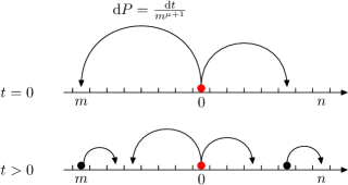
Figure 3.2: An illustration of the dynamics of the epidemics dynamics model of [208] in $d=1$. Initially ($t=0$), the only occupied site at $n=0$ infects other sites at a rate that decays as eq. (3.5). Later, $t>0$, infected sites go on to infect remaining sites.

Fisher and Hallatschek studied in [208] an epidemic dynamics model, which can be viewed as the long–range version of the Eden model introduced in section 1.3. It can be defined on a lattice in any dimension, and we shall restrict to $d=1$. For this, consider a linear lattice made of sites $n=-N/2,\dots,N/2-1$. Like the Eden model, every site can be either empty or occupied (infected). The dynamics is as follows, see Figure 3.2 for an illustration:

• Initially, at $t=0$, only the site $0$ is occupied, and all the others are empty.

• During each infinitesimal time interval $\mathrm{d}t$, and for any pair of sites $m$ and $n$, such that $m$ is occupied and $n$ is empty, $n$ becomes occupied with probability

  $$\mathrm{d}P_{mn}=\left|m-n\right|^{-\mu-1}\mathrm{d}t\,,$$ (3.5)

  That is, occupied sites “infect” all other sites with a rate that decays algebraically as function of the distance. All these events are uncorrelated.

• Once a site is occupied, it remains so forever.

The work [208] required $\mu>0$ in eq. (3.5) so that $\sum_{m}P_{mn}$ does not diverge in the infinite system $N\to\infty$ limit. In the epidemic dynamics context, the divergence would be unrealistic because the total rate at which a site send offspring elsewhere must be finite.

The main question treated in [208] is: how does the size of the colony (the set of occupied sites), $L(t)$, grows as a function of time (for $t\to\infty$)? The answer turned out to be quite non–trivial, and enjoys a rich dependence on the value of $\mu$. To get a feeling, let us consider the extreme cases:

• As $\mu\to\infty$, $\mathrm{d}P_{mn}=\mathrm{d}t$ if and only if $\left|m-n\right|=1$, and vanishes otherwise. So the model becomes a short–range one: the 1d Eden model. Trivially, the colony is always a full interval whose size grows linear in time: $L(t)=2t$, because only the sites at the boundary can infect its nearest neighbour: all other attempts are suppressed.

• When $\mu\to 0$, $\sum_{m}\mathrm{d}P_{mn}$ becomes divergent at $\left|m-n\right|$ large. The model is then approximatively “infinite–range”, in which all attempts increase actually $L(t)$. Since the number of attempts is proportional to $L(t)$, $L(t)=e^{ct}$ grows exponentially.

Now, for intermediate values of $\mu$, [208] showed that

$$L(t)\stackrel{{\scriptstyle t\to\infty}}{{\propto}}\begin{dcases}t\,,&\mu>2\,,\\ t^{\frac{1}{\mu-1}}\,,&\mu\in(1,2)\,,\\ \exp(ct^{\eta})\,,&\mu\in(0,1)\,,\\ \end{dcases}\quad\text{ where }\eta(\mu)=\log_{2}\left(\frac{2}{\mu+1}\right)\,.$$ (3.6)

Observe that the short–range behaviour extends to all values $\mu>2$. This condition equivalent to the condition that $\sum_{m}m^{2}\mathrm{d}P/\mathrm{d}t=\sum_{m}m^{-\mu+2}$ converges at $m\to\infty$. This means that the dispersion of offspring has a finite diffusion constant [208]. When $\mu<2$, the diffusion becomes anomalous (Lévy flights), and it is expected the colony size grows supra-linearly. In particular, the algebraic regime $\mu\in(1,2)$ can be understood by dimensional analysis [208]. For this, we notice that if the model were defined in the continuum, then eq. (3.5) would read

$$\mathrm{d}P=\left|x-y\right|^{-\mu-1}\mathrm{d}t\mathrm{d}x\mathrm{d}y\,,$$ (3.7)

where $x,y$ are continuous spatial coordinates, with the same dimension as $L$, while the left hand side is dimensionless. Therefore eq. (3.7) implies $[1]=[L]^{-\mu+1}[t]$, which is the same power law as the $\mu\in(1,2)$ case of (3.6) . However, there is another non–trivial qualitative change at $\mu=1$, and an exponential regime at $\mu(0,1)$, which cannot be explained by dimensional analysis (which fails at $\mu=1$). As we shall discuss in section 3.2.3, the colony grows in a fundamentally different way in this regime.

3.2.2 First–passage percolation

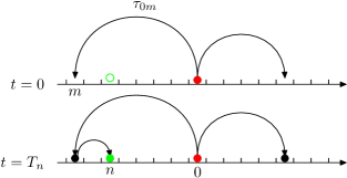
Figure 3.3: An illustration of the long–range first–passage percolation model and its correspondence to the epidemics model, see also Figure 3.2. For each pair of vertices (like $0$ and $m$ in the top panel), one assigns a waitiing time $\tau_{0m}$ which is an exponential random variable of mean value $\left|m\right|^{\mu+1}$, see eq. (3.8). Then one studies the first passage time $T_{n}$, defined as the first moment when $n$ is infected (bottom panel).

As we have seen in section 1.3, the Eden growth model is equivalent to a first–passage percolation (FPP) model. The same can be said about the epidemic dynamics model just discussed, which gives rise to a long–range first–passage percolation (FPP) model. This model is defined by a symmetric matrix of independent random waiting times $\tau_{mn}$ having exponential distribution:

$$\tau_{nn}\equiv+\infty\,,\,\mathbb{P}(\tau_{m\neq n}>t\geq 0)=\exp\left(-\frac{t}{\left|m-n\right|^{\mu+1}}\right)\,.$$ (3.8)

The relation with the epidemic model is ensured by the fact that the mean waiting time $\overline{\tau_{mn}}$ is the inverse of the rate $\mathrm{d}P_{mn}/\mathrm{d}t$ in eq. (3.5). The key observable is the first passage time, $T_{n}$, defined as the moment when the site $n$ becomes occupied. To define the $T_{n}$ in terms of $\tau_{mn}$, let us call a path (polymer) between two points $0$ and $m$ any finite sequence of sites $\mathfrak{p}=(0=m_{0},m_{1},\dots,m_{s}=n)$, $s$ being its length, $s=s[\mathfrak{p}]$. Note that the paths are not directed and the sites can be visited multiple times. The total waiting time of a path is defined as the sum over the edges

$$T[\mathfrak{p}]=\sum_{i=1}^{s}\tau_{m_{i},m_{i-1}}\,.$$ (3.9)

Then, the following analogue of eq. (1.17) holds

$$T_{n}=\min_{\mathfrak{p}:0\rightarrow n}T[\mathfrak{p}]\,.$$ (3.10)

Because of the long–range dispersion, the minimum is over any paths. The fundamental question is to determine how $T_{n}$ grows as a function of $n$.

This question is answered rigorously by Chatterjee and Dey [209] (the work was independent to Fisher–Hallatscheck’s [208]), and the answer reads as

$$T_{n}\stackrel{{\scriptstyle n\to\infty}}{{\propto}}\begin{dcases}\left|n\right|\,,&\mu>2\,,\\ \left|n\right|^{\mu-1}&\mu\in(1,2)\,,\\ \exp\left(c\sqrt{\ln\left|n\right|}\right)&\mu=1\,,\\ \left(\ln\left|n\right|\right)^{\kappa(\mu)}\,,&\mu\in(0,1)\\ O(1)\,,\,&\mu\leq 0\,,\end{dcases}\quad\text{ where }\kappa(\mu)=\frac{\ln 2}{\ln\frac{2}{\mu+1}}=\eta(\mu)^{-1}\,,$$ (3.11)

where $\eta(\mu)$ is defined in (3.6). One can check that $T_{n}$ and $L(t)$ are inverse functions of each other in all cases when they can be compared, which is expected. The $\mu=1$ case is a marginal case that is also obtained in [208]. The $\mu\leq 0$ result justifies excluding this regime from the epidemics point of view: the growth of $L(t)$ is not exponential, but spontaneous (an exponential growth requires carefully logarithmic fine–tuning of eq. (3.8), as shown in [209]).

3.2.3 Stretch-exponential regime

Let us explain the results (3.11) or (3.6) in the stretch exponential regime $\mu\in(0,1)$, following [208]. This regime is especially important because it is the inspiration of our original arguments in section 3.4.2.

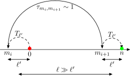
Figure 3.4: An illustration of the typical minimizing path in the $\mu\in(0,1)$ regime. It is made of a long bond $m_{i},m_{i+1}$ of length $\ell_{k}\sim\left|n\right|$, and two sub–polymers (drawn in dashed curves) connecting $0\to m_{i}$ and $m_{i+1}\to n$, each of which repeating the structure.

The key characteristics of the stretch exponential regime is the structure of the minimizing path of eq. (3.10), denoted $\mathfrak{p}=(0=m_{0},\dots,m_{s}=n)$, see Figure 3.4 for illustration. It has typically a bond $m_{i},m_{i+1}$ of length $\left|m_{i}-m_{i+1}\right|\sim\ell=\left|n\right|$ comparable to the distance between two end–points, and such that $\tau_{m_{i},m_{i+1}}\sim O(1)$. According to eq. (3.8), the probability that this happens for one bond length $\ell$ is $\ell^{-\mu-1}\ll 1$. However, if one defines the following scale

$$(\ell^{\prime})^{2}\ell^{-\mu-1}=1\Leftrightarrow\ell=(\ell^{\prime})^{\frac{2}{\mu+1}}\ll\ell$$ (3.12)

when $\mu<1$ and $\ell\gg 1$, then the minimum of the set of $4\ell^{\prime 2}$ bonds, $\tau_{mm^{\prime}}$ for $\left|m\right|\leq\ell^{\prime}$ and $\left|m-n\right|\leq\ell^{\prime}$, will be an exponential random variable of mean value $1/4$. So there must be some $m,m^{\prime}$ that can play the rôle of $m_{i},m_{i+1}$. However, we have no control over their distance from $0$ (and $n$, respectively) other than $\left|m-0\right|,\left|m^{\prime}-n\right|\sim\ell^{\prime}$. Thus, the waiting time two halves of the polymers $0\to m$ and $m^{\prime}\to n$ can be estimated by $T_{\ell^{\prime}}$. Summarizing, we have the following recursion relation for $T_{\ell}$

$$T_{\ell}=T[\mathfrak{p}]=\underbrace{\tau_{m_{i},m_{i+1}}}_{O(1)}+\underbrace{\sum_{j=1}^{i}\tau_{m_{j},m_{j-1}}}_{T_{\ell^{\prime}/2}}+\underbrace{\sum_{j=i+1}^{s-1}\tau_{m_{j},m_{j+1}}}_{T_{\ell^{\prime}/2}}\sim 2T_{\ell^{\prime}}\,.$$ (3.13)

Now, both eq. (3.12) and (3.13) can be repeated. When $\mu<1$, eq. (3.12) defines a sequence of lengths

$$\ell_{k}=\ell_{k-1}^{\frac{2}{\mu+1}}\Rightarrow\ln\ell_{k}=\left(\frac{2}{\mu+1}\right)^{k}\ln\ell_{0}\Rightarrow\ln\ln\ell_{k}=\ln\ln\ell_{0}+k\ln\frac{2}{\mu+1}$$ (3.14)

where $\ell_{0}>1$ can be fixed arbitrary. On the other hand, eq. (3.13) implies

$$T_{\ell_{k}}=2^{k}T_{\ell_{0}}\Rightarrow\ln T_{\ell_{k}}=\ln T_{\ell_{0}}+k\ln 2\,.$$ (3.15)

Combining eq. (3.14) and (3.15) to eliminate $k$, we recover the $\mu\in(0,1)$ case of eq. (3.11), namely:

$$\ln T_{\ell}=\frac{\ln 2}{\ln\frac{2}{\mu+1}}\ln\ln\ell+c\Rightarrow T_{\ell}=\left(\ln\ell\right)^{\kappa(\mu)}\,.$$

Note that such a strategy is not possible when $\mu\geq 1$ because eq. (3.12) would imply $\ell^{\prime}\gg\ell$.

In terms of the epidemic dynamics, the above discussion entails that when $\mu<1$, the colony grows in an explosive manner: from time to time, the colony sends a offspring to a distance which is far greater than the present colony size. The offspring becomes the seed of a new satellite. The colony growth is dominated by the multiplication of satellites. In contrast, when $\mu>1$, the growth is incremental, in the sense that the dominating dispersion length is much smaller than then the colony size.

3.3 Beta Banded Random Matrices (BBRM)

3.3.1 Motivation, definition and main results

In this section, we study the Beta Banded Random Matrices (BBRM), following [5]. Before defining it, we summarize the two motivations behind it.

• The first motivation is to find better 1D long–range proxies than PBRM for the Anderson localization transitions in $d>2$ dimensions. As we have seen in section 3.1.2, the phase diagram of PBRM is oversimplified because direct hopping dominates the transport in the space that PBRM describe. Moreover, the argument that leads to the phase diagram is quite general. Indeed, the PBRM’s phase diagram would not be changed if we changed the distribution of its matrix elements to

  $$P(H_{mn})=\sqrt{g}P_{0}(\sqrt{g}H)\,,\,g=\beta\left|n-m\right|^{1+\mu}\,,\,\left|m-n\right|\gg 1\,,$$ (3.16)

  where $P_{0}$ is any narrow enough distribution (e.g., uniform in $[-1,1]$) such that the moments obey

  $$\overline{H_{mn}^{p}}\propto g^{-p/2}\,,\,\left|m-n\right|\gg 1\,,\,p=1,2,3\dots.$$ (3.17)

  This means that all matrix elements corresponding to a certain (large) distance $|n-m|$ have the same order of magnitude $g_{mn}^{-1/2}$. So, in order to change the phase diagram, a natural direction is to look at banded random matrices whose elements’ distribution is radically different.

• The second motivation is that the long–range epidemics/FPP model gives rise naturally to BBRM via a mapping, and the results and methods of [208, 209] (discussed in section 3.2) lead to predictions on BBRM. This mapping will be explained in section 3.3.3.

Now let us define the BBRM. It is inspired directly by the long range FFP model in section 3.2.2. Formally, it can be defined as

$$Q_{nm}=\exp(-\beta\tau_{nm})\,,\,n,m=1,\dots,N\,,$$ (3.18)

where $\tau_{nm}$ is the matrix of waiting times eq. (3.8), and $\beta$ is the extra parameter of the matrix model. Equivalently, the BBRM ensemble is defined as a real symmetric $N\times N$ matrix whose diagonal entries are all ro ($Q_{nn}\equiv 0$) and all off-diagonal entries $Q_{nm}$ are independent random variables in $(0,1)$, with a Beta distribution,

$$\mathbb{P}(Q_{mn}<q)=q^{1/g}\,,\,g=\beta\left|m-n\right|^{\mu+1}\,,\,q\in(0,1)\,.$$ (3.19)

So the BBRM model has the same parameters $\mu,\beta$ as PBRM.

Figure 3.5: Taken from [5]. Schematic phase diagram of BBRM s. The decay of the eigenstates $\phi$ in different regimes are indicated. In the regime $\mu\in(0,1)$, there is a mobility edge $\lambda(\beta;\mu)$ (blue curves) separating localized eigenstates (red region) and extended eigenstates (green region). The localized states have a very peculiar decay, Eq. (3.20). When $\mu>1$, all the eigenstates are localized, but with a stretched exponential decay for $\mu<2$, Eq. (3.21).

We now summarize the main results of [5] on this model (see Figure 3.5):

• When $\mu\in(0,1)$, the model enjoys a localization transition with mobility edges, separating extended states in the middle of the spectrum from localized states elsewhere. This is the most important result of [5]. We will discuss it in section 3.3.4.

• When $\mu\in(0,1)$, the localized states have a peculiar decay. Indeed, if $\phi_{m}$ is a states localized around $m$, we have

  $$\left|\langle n|\phi_{m}\rangle\right|=\exp\left(-C\ln^{\kappa(\mu)}(\left|n-m\right|/\xi)\right)\,,\,\text{ where }\kappa(\mu)=\frac{\ln 2}{\ln(2/(\mu+1))}$$ (3.20)

  is the same exponent as in (3.11).

• When $\mu>1$, all eigenstates are localized, with a stretch exponential decay:

  $$\left|\langle n|\phi_{0}\rangle\right|\sim\exp\left(-C\left|n\right|^{\min(\mu,2)-1}\right)\,,\,\mu>1\,.$$ (3.21)

  The predictions eq. (3.21) and (3.20) come from the mapping to FPP model, as will discuss in section (3.3.3).

3.3.2 Basics: broad distribution, density of states

This section discusses two elementary aspects of BBRM that are preliminary to further investigations.

Broad distribution of matrix elements

First, let us recall some basic statistical properties of its matrix elements:

$$\mathbb{P}(Q_{mn}<q)=q^{1/g}\,,\,g=\beta\left|m-n\right|^{\mu+1}\,,\,q\in(0,1)\,.$$ (3.22)

Note that the dependence on $m,n$ and $\beta$ is through $g$. When $g=1$, $Q_{mn}$ is uniformly distributed, when $g\rightarrow 0$, $Q_{mn}\rightarrow 1$ becomes non-random. This justifies calling $\beta\rightarrow 0$ the weak disorder limit, and $\beta\rightarrow\infty$ the strong disorder limit consequently.

Figure 3.6: Taken from [5]. The magnitudes of matrix elements of PBRM (line) and BBRM (dots) on one line of the matrix,as a function of the distance from the diagonal. For both matrices, we used the parameters $\mu=.5,\beta=0.1$. The red dashed line depicts the standard deviation common to both. Many elements of the BBRM are too small to be drawn on the plot.

It is the behaviours of $Q_{mn}$ as $g\to\infty$ that are crucially different from that of PBRM. Indeed, it is an example of what we shall call broad distributions in section 3.4: the typical value $Q_{mn}$ is very small compared to its integer moments, which are contributed by occurrences of black swans of magnitude $O(1)$ with probability $1/g$ (see Figure 3.6). More quantitatively,

• Its moments are

  $$\overline{Q_{mn}^{k}}=\frac{1}{1+kg}\,,$$ (3.23)

  $$\overline{\exp(-tQ_{mn})}=\sum_{k=0}^{\infty}\frac{(-t)^{k}}{k!}\frac{1}{1+kg}=g^{-1}t^{-1/g}(\Gamma(1/g)-\Gamma(1/g,t))\,.$$ (3.24)

  where $\Gamma(x,z)=\int_{z}^{+\infty}\mathrm{d}ye^{-y}y^{x-1}$ is the incomplete Gamma function. As a consequence, the second moment of BBRM matrix elements have the same decay as PBRM, eq. (3.3). However, all its integer moments decay as $1/g$, which is different from eq. (3.17).

• $Q_{mn}$ can be characterised by the property that $-\ln Q_{mn}$ is exponentially distributed with mean value $g$ (see also eq. (3.18)):

  $$\mathbb{P}(-\ln Q_{mn}>l)=\exp(-l/g)\,,\,l\geq 0\,.$$ (3.25)

  Therefore, its typical value, defined as the exponential of the mean of log, is

  $$Q^{\text{typ}}_{mn}\stackrel{{\scriptstyle\text{def}}}{{=}}\exp(\overline{\ln Q_{mn}})=\exp(-g)\,.$$ (3.26)

  As $g\rightarrow\infty$, $Q^{\text{typ}}_{mn}\ll\overline{Q^{k}_{mn}}$. The same can be said about its median, which is $m(Q_{mn})=\exp(-g\ln 2)$.

• Eq. (3.25) implies also that the occurence probability of black swans

  $$\mathbb{P}(Q_{mn}>a)\sim\frac{-\ln a}{g}\,,\,g\rightarrow\infty\,,0<a<1\text{ fixed.}$$ (3.27)

In summary (see also Figure 3.6), when the parameters $\mu$ and $\beta$ are the same, BBRM’s typical matrix elements decay in fact faster than PBRM, yet the latter does not have the atypically large elements of BBRM.

Density of states (DoS)

It is always helpful to have an idea of the density of states (DoS)of the random matrix model at hand. The general definition of the DoS for any random matrix is:

$$\rho(\lambda)=\frac{1}{N}\sum_{i=1}^{N}\overline{\delta(\lambda-\lambda_{i})}\,,$$ (3.28)

where $\lambda_{1},\dots,\lambda_{N}$ are the eigenvalues of the matrix. When averaged over disorder, $\rho(\lambda)$ is usually a continuous function that vanishes outside some finite interval $[\lambda_{-},\lambda_{+}]$ (a notable exception is the Lévy matrix [210, 211], for which $\lambda_{+}=+\infty$). For example, we recall [201] that the DoS of the PBRM is always given by Wigner’s semi–circle law (upon a rescaling)

$$\rho(\lambda)=\frac{2}{\lambda_{+}\pi}\sqrt{1-(\lambda/\lambda_{+})^{2}}\,.$$

Figure 3.7: Taken from [5]. Left: Rescaled DoS $\rho(\hat{\lambda})$ of the BBRM for $\mu=-.5$ and $\beta=1$, where $\hat{\lambda}=a+b\lambda$ is the rescaled eigenvalue so that the mean and variance are that of the semicircle law. Right: DoS of the BBRM for $\mu=.5$ and various $\beta$. The curve $\beta=20$ is compared to the prediction eq. (3.29), plotted in dashed line.

In general, the width of the support of the DoS can be estimated by

$$\overline{\lambda^{2}}\stackrel{{\scriptstyle\text{def.}}}{{=}}\int\rho(\lambda)\lambda^{2}\mathrm{d}\lambda=\frac{1}{N}\sum_{i}\overline{\lambda_{i}^{2}}=\frac{1}{N}\overline{\mathrm{Tr}\hat{H}^{2}}=\frac{1}{N}\sum_{nm}\overline{H_{mn}^{2}}$$

For both PBRM and BBRM, the last quantity $\sim\sum_{n=1}^{N}\beta^{-1}\left|n\right|^{-\mu-1}$ (by eq. (3.23) and eq. (3.17)). So, when $\mu<0$, $\overline{\lambda^{2}}\sim N^{-\mu}$ diverges as $N\to\infty$. In such cases, according to a theorem of [212], BBRM’s density of state must also be a semicircle law. This is corroborated by the numerical measure, which we show in Figure 3.7 (left panel).

However, when $\mu>0$, due to the absence of diagonal disorder ($Q_{nn}=0$), its DoS $\rho(\lambda)$ is in fact quite peculiar. It develops a divergence at $\lambda=0$, and a non-analyticity at $\lambda=\pm 1$ as $\beta$ increases. For $\beta\gg 1$, most elements are vanishing, and a crude estimate of DoS is given by the distribution of the eigenvalues $\pm Q_{01}$ of the $2\times 2$ sub-matrix $\begin{pmatrix}0&Q_{01}\\ Q_{01}&0\end{pmatrix}$. This leads to:

$$\rho(\lambda)\approx\left|\lambda\right|^{-1+1/\beta}/(2\beta)\,,\,\text{ if }\left|\lambda\right|<1$$ (3.29)

and $\rho(\lambda)\approx 0$ for $\left|\lambda\right|>1$. In Figure 3.7 (right panel), we show a numerical check of this claim. We observe also that even for $\beta\sim 1$, the DoS of BBRM differs significantly from the semi–circle law.

3.3.3 Mapping to the epidemic dynamics

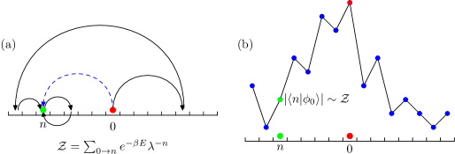
Figure 3.8: The relation between the polymer model and Anderson localisation. (a) In the polymer model, which is a finite temperature extension of the growth model, we sum over all paths connecting two points $0$ and $n$, ranging from the direct path (blue, dashed) and detoured paths with loops, for example, the one in black. (b) The amplitude at site $n$ of (strong-disorder) BBRM eigenstates localized around $0$ is in turn related to the polymer partition function by (3.36).

This section, based on [5] (Supplemental Material, section D), will explain the relation between the BBRM and the long–range FPP model, and then use it to derive the decay rate of the localized states of BBRM, eq. (3.21) and (3.20).

The relation between BBRM and the long–range FPP follows directly from the relation of the long–range FPP and a statistical model of long–range “polymers” in random media, analogous to the one discussed in section 1.3. The latter polymer model is defined by a grand canonical partition function $\mathcal{Z}$ which is a sum over all the paths from $0$ to $n$, with energy given by eq. (3.9). The inverse temperature is $\beta$, and the chemical potential associated to the length of the polymer will be denoted $\tau$ (to avoid clash with $\mu$). Namely, we have (see Figure 3.8, (a) for an illustration)

$$\mathcal{Z} =\sum_{s=0}^{\infty}\sum_{\begin{subarray}{c}\mathfrak{p}:(m_{0},\dots,m_{s})\\ m_{0}=0,m_{s}=n\end{subarray}}\exp(-\beta T[\mathfrak{p}]+s\beta\tau)$$

$$=\sum_{s=0}^{\infty}\sum_{m_{1}}\dots\sum_{m_{s-1}}\exp\left(-\beta\sum_{i=1}^{s}(\tau_{m_{i}m_{i-1}}-\tau)\right)\,.$$ (3.30)

This is the long–range version of the polymer model, defined in eq. (1.18) of section 1.3. Now, using eq. (3.18) and the definition of matrix multiplication, eq. (3.30) can be written as a resolvent of the BBRM

$$\mathcal{Z} =\sum_{s=0}^{\infty}\sum_{m_{1}}\dots\sum_{m_{s-1}}\prod_{i=1}^{s}\left(Q_{m_{i}m_{i-1}}\lambda^{-1}\right)=\langle n|(1-\hat{Q}/\lambda)^{-1}|0\rangle\,,\,\lambda=e^{-\beta\tau}\,,$$ (3.31)

On the other hand, The zero–temperature, zero–chemical potential limit of the free energy is just the first passage time $T_{n}$ defined in eq. (3.10) (this is a long–range analogue of eq. (1.19)):

$$T_{n}=\left[-\beta^{-1}\ln\mathcal{Z}\right]_{\beta\to\infty,\tau\to 0}=\left[-\beta^{-1}\ln\left|\langle n|(1-\hat{Q}/\lambda)^{-1}|0\rangle\right|\right]_{\beta\to\infty,\tau\to 0}\,,$$ (3.32)

where we applied eq (3.31). This equation allows to translate the known asymptotic growth of $T_{n}$ (eq. (3.11)) to the decay of eigenstates in the strong disorder $\beta\to\infty$ limit. To this end, let us fix some $\lambda\neq 0$ while let $\beta\to\infty$, so $\tau=-\beta^{-1}\ln\lambda\to 0$ by eq. (3.31). So eq. (3.32) can be rewritten as

$$\ln\left|\langle n|(1-\hat{Q}/\lambda)^{-1}|0\rangle\right|\stackrel{{\scriptstyle\beta\gg 1}}{{\approx}}-\beta T_{n}\,,\,\lambda\neq 0\,.$$ (3.33)

The decay of the left hand side is related that of eigenstates in a quite standard way, as we briefly review. For this, we write $\hat{Q}$ in the basis of its eigenstates $|\lambda^{\prime}\rangle$ of $\mathbf{Q}$ (with energy $\lambda^{\prime}$):

$$\langle n|(1-\hat{Q}/\lambda)^{-1}|0\rangle=\sum_{\lambda^{\prime}}\frac{\langle n|\lambda^{\prime}\rangle\langle\lambda^{\prime}|0\rangle}{1-\lambda^{\prime}/\lambda}\,.$$ (3.34)

Because of the denominator, the sum is dominated by eigenstates with energy close to $\lambda$, and the decay of those eigenstates determines the behaviour $\langle n|\lambda^{\prime}\rangle\langle\lambda^{\prime}|0\rangle$ as a function of $n$. Indeed, when $|\lambda^{\prime}\rangle$ is localized around some site $m$ with decay $\ln\left|\langle n|\lambda^{\prime}\rangle\right|\propto-T_{\left|m-n\right|}$, we have $\ln\left|\langle n|\lambda^{\prime}\rangle\langle\lambda^{\prime}|0\rangle\right|=-T_{\left|m\right|}-T_{\left|n-m\right|}\leq-T_{\left|n\right|}$ (the last convexity inequality can be checked for all cases of eq. (3.11)), so the eigenstates localized at $0$ or $n$ will dominate (3.34) and give the same contribution:

$$\ln\left|\langle n|(1-\hat{Q}/\lambda)^{-1}|0\rangle\right|\approx\ln\left|\langle n|\phi_{0}\rangle\right|\,,$$ (3.35)

where $|\phi_{0}\rangle$ is an eigenstate localized around $0$ having energy $\approx\lambda$. Combined with (3.33), we have

$$-\ln\left|\langle n|\phi_{0}\rangle\right|\stackrel{{\scriptstyle\beta\gg 1}}{{\approx}}\beta T_{n}\,,\,$$ (3.36)

In particular, if $T_{n}$ does not increase with $\left|n\right|$, the state $|\phi_{0}\rangle$ in fact extended (this is the case when $\mu<0$). As we have noted, the above equation is valid for $\lambda\neq 0$. More precisely, the requirement is that $\tau=\left|\beta^{-1}\ln\lambda\right|\ll 1$. So for a given large $\beta$, eq. (3.36) covers the whole spectrum except an exponentially small interval $(-e^{-c\beta},e^{-c\beta})$ around $0$.

$\mu\in$	$T_{n}\propto$	BBRM $\left|\langle n|\phi_{0}\rangle\right|\sim$	PBRM $\left|\langle n|\phi_{0}\rangle\right|\sim$
$(-1,0]$	$\stackrel{{\scriptstyle L\rightarrow\infty}}{{\longrightarrow}}0$	extended	extended
$(0,1)$	$\left(\ln\left|n\right|\right)^{\kappa(\mu)}$	$\exp\left(-c\ln^{\kappa(\mu)}\left|n\right|\right)$/extended	extended
$\{1\}$	$e^{c\sqrt{\ln\left|n\right|}}$	$\exp\left(-e^{c\sqrt{\ln\left|n\right|}}\right)$ / extended	critical
$(1,2)$	$\left|n\right|^{\mu-1}$	$\exp\left(-c\left|n\right|^{\mu-1)}\right)$	$\left|n\right|^{-(\mu+1)/2}$
$(2,\infty)$	$\left|n\right|$	$\exp\left(-c\left|n\right|\right)$	$\left|n\right|^{-(\mu+1)/2}$

Table 3.1: Summary of asymptotic first-passage time [208, 209] of the first-passage percolation model and their implication on the eigenstate decay of BBRM. $\kappa(\mu)=\ln 2/\ln\frac{2}{\mu+1}$. The results on PBRM [201] are also shown to compare. In the $\mu\in(0,1)$ regime, BBRM has localization transitions and extended eigenstates, see section 3.3.4. In the $\mu<0$ regime, $T_{n}\rightarrow 0$ in the $L\rightarrow\infty$ limit. By (3.36), this means the eigenstates are extended even in the $\beta\gg 1$ limit.

In Table 3.1, we list the results eq. (3.11) and their translation by (3.36). In particular, eq. (3.21) and (3.20) are contained in the cases $\mu>1$ and $\mu\in(0,1)$, respectively. We also quoted the analogous results for the PBRM, known in [201]. Note that BBRM eigenstates decay always faster than PBRM ones. In particular both BBRM and PBRM eigenstates are all localized when $\mu>1$, the decay are qualitatively different. The PBRM eigenstates are always algebraically decaying, and the decay rate is simply by the typical magnitude of the hopping element $\left|H_{0n}\right|\sim\left|n\right|^{-(\mu+1)/2}$. On the other hand, the BBRM eigenstates have an exponential decay when $\mu\geq 2$, recovering the short–range Anderson model behaviour. For $\mu<1$, as we show in [5] (Supplemental Material, section E), the non–trivial decay rates of BBRM can be interpreted in terms of Anderson models in higher dimensions.

The alert Reader may have noticed that eq. (3.36) makes only predictions in the $\beta\gg 1$ strong disorder limit, and we have tacitly extended them to all localized eigenstates. The usual argument supporting this is a scaling/renormalization group one like that in [200]: as long as one is in the localized phase, even when the disorder is weak ($\beta$ not large), its behaviour at sufficient large scale flows to the $\beta\to\infty$ fixed point. Moreover, in [5], we measured numerically the decay of eigenstates of BBRM with various values of $\mu>1$, with $\beta=.25$, and compared to eq. (3.21) (see Figure 3.9 for numerics details and data). The results confirm the assertion that the predictions in the strong disorder limit do extend to small $\beta$. The same test is much less conclusive in the $\mu\in(0,1)$ regime, because not all eigenstates are localized: there is a localization transition. We claimed this in section 3.3.1 (see Figure 3.5), and will start discussing it in the next section 3.3.4.

Figure 3.9: Taken from [5]. Numerical test of the (stretched) exponential decay of the localized states of BBRM for . The prediction eq. (3.21) is plotted as lines for $\mu=2.5,1.8,1.5,1.2$ (from top to bottom). To obtain the numerical data, we diagonalize BBRM s of size $N\times N$, $N=2^{11}$, with $\beta=.25$, and retain the $N/4$-th to $3N/4$-th eigenstates (ordered by eigenvalue) of each realisation. For each eigenstate $|\phi\rangle$, we define its localization centre $n_{\max}$ as the site with maximum amplitude $\left|\langle\phi|{n}\rangle\right|$. We then obtain the distribution of $\ln\left|\langle\phi|n_{\max}\rangle/\langle\phi|n\rangle\right|$ for each $\left|n-n_{\max}\right|$, and plot the median as data points.

Contextual remark

We remark that the mapping above is a new instance of the well–known interplay between polymer in random media and localization [213, 214, 215, 211]. A highlight of this connection has been the relation between the conductance fluctuations in the short-range 2D Anderson model to the $(1+1)$-d KPZ [17] universality class [28, 216, 217]. As we have seen in 1.3, the $(1+1)$-d KPZ class is believed of govern the fluctuations of the first–passage time $T(x,y)$ in the short range Eden growth model in 2D. More precisely, denoting $x,y=r\cos\theta,r\sin\theta$, we have

$$T(x,y)=a(\theta)r+br^{1/3}\chi_{TW}\,,r\to\infty\,.$$ (3.37)

So the leading behaviour is linear $\propto r$, while $a(\theta)$ is some non-universal function controlling the limit shape of the colony. The fluctuation around $a(\theta)$ has the $(1+1)$-d KPZ universal scaling $r^{1/3}$ (but $b$ is a non–universal pre–factor), and $\chi_{TW}$ is a universal Tracy–Widom distribution (see [18] for review of the KPZ universality class in $(1+1)$-d and beyond). Note that eq. (3.37) is another instance of the statistics Ansatz eq. (1.2). In [216], it is shown that the log–conductance of the 2D Anderson’s model in the insulator phase, as a function of the length $r$ of the sample, satisfies also eq. (3.37) (further observation of other universal KPZ predictions was made in [217]). Assuming that the conductance is essentially given by the resolvent eq. (3.34), these results are to be expected in light of the mapping of this section.

For the long–range model considered here, it is the leading behaviour that becomes non–trivial functions of $n$, as given by $T_{n}$ in Table 3.1. The fluctuation laws are not known yet.

3.3.4 Localization transition

The existence of localization transition and extended state in BBRM with $\mu\in(0,1)$ is the main claim of [5]. In this section, we shall support the claim with a first, heuristic, argument based on long–range percolation, and with numerical simulations. In section 3.4, another more general argument will be presented.

Long–range percolation argument

This argument, presented in [5] (main text and Supplemental Material, section D), concerns the BBRM in the strong disorder $\beta\gg 1$ regime. It starts with the observation that the grand canonical partition function eq. (3.31) is an infinite series that can diverge. Indeed, for any pair $m,m^{\prime}$, the sub-series made up back–and–forth paths $(0,m,m^{\prime},m,m^{\prime},\dots,m,m^{\prime},n)$, $\ell=1,2,\dots$, which is $Q_{0m}Q_{m,m^{\prime}}Q_{m^{\prime}n}\lambda^{-3}\sum_{k=0}^{\infty}(Q_{mm^{\prime}}/\lambda)^{2k}$, diverges when

$$Q_{mn}>\lambda=e^{-\beta\tau}\Leftrightarrow\tau_{mn}<\tau\,,$$ (3.38)

see eq. (3.30). Such a divergence is associated with condensation phenomena in statistical physics. At the onset of divergence $Q_{mn}=\left|\lambda\right|-\varepsilon$, the “polymer” tends to occupy infinite number of times on the link $m\leftrightarrow m^{\prime}$. Beyond that point, the statistical mechanics model is non–physical. However, from the quantum mechanics (matrix eigenstates) point of view, such divergence should be re-summed and interpreted as a resonance between the sites $m$ and $m^{\prime}$. From (3.8) and (3.38), one sees that the probability of such resonance is

$$p_{nm}=1-e^{-\tau/\left|n-m\right|^{\mu+1}}\sim\frac{\tau}{\left|n-m\right|^{\mu+1}}\,,\,\left|m-n\right|\to\infty\,.$$ (3.39)

The random graph made of resonating edges defines thus a long–range percolation problem [218].

When $\tau=0$ ($\lambda=1$), the graph is completely disconnected; when $\tau=\infty$, the graph is completely connected. In the limit of large systems, a sharp percolation transition is expected at some $\tau_{c}$. When $\tau<\tau_{c}$, we have the “insulating” phase, where connected clusters of the graph are of finite size. When $\tau>\tau_{c}$, we have the “percolating” phase, where infinite clusters appear. A necessary criterion for the existence of the percolating phase at finite $\tau$ is the presence of a resonance crossing any site $i$, of the system. This probability is given by

$$p_{i}=1-\prod_{n<0}\prod_{m>0}(1-p_{nm})=1-\exp(-\tau\sum_{\ell>0}\ell^{-\mu})$$

where $\ell=n-m$. So when $\mu>1$, the sum over $\ell$ is convergent and $p_{i}<1$, which makes percolation impossible (because one needs to accomplish infinitely many conditions with probability $p_{i}<1$). When $\mu<1$, on the other hand, $p_{i}=1$, and a percolation transition can occur; its existence was indeed proven in [219, 220].

Now, the percolation of the graph of resonance bonds is generally associated with the de-localization of the eigenstate. Therefore, the above results indicate that extended states cannot exist when $\mu>1$. When $\mu<1$, there are extended states with exponentially small eigenvalues $\left|\lambda\right|<\lambda_{c}\approx e^{-\beta\tau_{c}}$ as $\beta\rightarrow\infty$. Since we know from the mapping to FPP that the eigenstates with $\lambda\sim O(1)$ (as $\beta\to\infty$) are localized, we expect a localization transition with mobility edges, at position

$$\lambda_{c}\approx e^{-\beta\tau_{c}}\,,\beta\gg 1\,.$$ (3.40)

This argument is quite heuristic, because percolation does not necessarily imply de–localisation. For example, in 2D short–range lattices, percolation is possible, but the Anderson model does not have an extended phase . However, in our case, the estimate eq. (3.40) captures qualitatively the phase diagram seen in the numerics (see below): the extended phase is indeed in the middle of the spectrum, and its size shrinks (rapidly) as $\beta$ increases.

In the hindsight, we remark that a relation between BBRM and long–range percolation is not a surprise, because the latter is known to be closely related to the long–range FPP model that inspired our definition of the BBRM. Indeed, it has been shown [221, 222] that, if $0$ and $n$ are two lattice points that are connected in the long–range percolation model, then the formulas of $T_{n}$ in Table 3.1 describe also the asymptotic behaviour of the shortest path connecting them on the random graph. This observation will also inspire the generalization of the BBRM results to more general random matrices, in section 3.4.

Numerical study of the localization transition

There are two ways of numerically studying the localization transition: i. studying the eigenstates themselves, and ii. studying the level statistics of the eigenvalues.

The most common observable of the eigenstates is the (generalized) inverse participation ratio (IPR). Recall that for a normalised state $\phi$, it is defined as

$$P_{q}=\sum_{n=1}^{N}\left|\langle\phi|n\rangle\right|^{2q}\,.$$ (3.41)

It is the same definition as in eq. (2.80) in section 2.1.4, if we identify the Gibbs measure $p_{\beta,n}$ with the occupying probability $\left|\langle\phi|n\rangle\right|^{2}$.. The asymptotic behaviours (as $N\to\infty$) of $P_{q}$ the extended and localized phase are

$$P_{q}\sim\begin{dcases}N^{0}&\text{localized phase}\,,\\ N^{1-q}&\text{extended phase}\,.\end{dcases}$$ (3.42)

One can see this by studying the extreme cases. The most localized state is a single site state $|\phi\rangle=|n_{0}\rangle$, for which $P_{q}=1$ for any $q$. The most de-localized state is uniformly distributed, $|\phi\rangle=N^{-1/2}\sum_{n=1}^{N}e^{\mathbf{i}\theta_{n}}|n\rangle$, for which $P_{q}=N^{1-q}$ exactly. At the localization transition, $P_{q}\sim N^{-\tau_{q}}$ for some non-linear exponent function $\tau_{q}$ characterizing the multi–fractal properties of the critical eigenstate . In what follows, the term IPR refers to the case $q=2$, on which we focus exclusively.

Figure 3.10: Taken from [5]. Measure of the IPR of BBRM eigenstates as function of eigenvalue $\lambda$, at $\mu=0.5$ and with various size of matrices, $N=2^{7},\dots,2^{14}$ (darker colours indicate larger systems). According to eq. (3.42), extended (localised) states would have $y$ coordinate $-\overline{\ln P_{2}}/\ln N\to 1$ ($\to 0$, respectively) when $N\to\infty$. Left panel: $\beta=5$. Dashed lines indicate the mobility edges, estimated at $\lambda_{c}\approx-0.65(5)$ and $\lambda_{c}\approx 0.70(5)$; they are not accurate estimates, because of the pronounced correction to scaling effect: the crossing of curves move to the outside when $N$ increases. Taking into this effect, a crude estimate of the critical IPR is $\tau_{c}=\left[\overline{\ln P_{2}}/\ln N\right]_{\lambda_{c}}\approx 0.36(5)$. Right panel: The same measure for $\mu=0.5$, $\beta=1$. As $N$ increases (darker colour), the eigenstates with $\lambda\in(-3,3)$ becomes more and more de-localised.

In Figure 3.11 (Left panel), we show the numerical measure of the IPR $P_{2}$ for the BBRM ensemble with $\mu=0.5$, $\beta=5$. For this we generate samples of BBRM, and numerically diagonalize them (using LAPACK wrapped in the numpy package). We observe clear mobility edges separating extended states in the middle of the spectrum (containing $\lambda=0$) and localized states near the edges. We considered other values of $\beta$ than $5.0$. For larger values, the results are qualitatively the same, but the extended phase shrinks to the point $\lambda=0$. For $\beta\approx 1$ (see Figure 3.11, Right panel, the extended phase expands rapidly, and we cannot decide whether the mobility edges disappear or are located near the edge of the spectrum. Thus, we cannot exclude the existence of a value $\beta_{\inf}(\mu)$ such that all eigenstates are extended when $\beta<\beta_{\inf}$.

Now we turn to the level statistics. Because of the non-trivial shape of the DoS (see Figure 3.7), the most suitable observable is the gap ratio proposed in [223]. Denoting $\lambda_{1}\leq\dots\leq\lambda_{N}$ the ordered eigenvalues of a matrix, and $\delta_{i}=\lambda_{i+1}-\lambda_{i}$ the level spacings (gaps), we consider the following ratio between successive gaps

$$r_{i}=\min(\delta_{i},\delta_{i+1})/\max(\delta_{i},\delta_{i+1})\,.$$ (3.43)

The advantage of this observable is that it cancels out the dimension of energy, and does not depend on the DoS. Its mean value is universal in localized and extended phases [224]

$$\overline{r}=\begin{dcases}r_{P}=2\ln-1\approx 0.39&\text{localized phase}\,,\\ r_{GOE}\approx 4-2\sqrt{3}\approx 0.53\,,&\text{extended phase}.\end{dcases}$$ (3.44)

The localized value $r_{P}$ comes from Poisson level statistics, while in the extended phase, $r_{GOE}$ is the value of the GOE ensemble; its approximate and numerical values were studied in [224]. It is then convenient to define the rescaled gap ratio

$$\chi\stackrel{{\scriptstyle\text{def.}}}{{=}}\frac{\overline{r}-r_{P}}{r_{GOE}-r_{P}}\Rightarrow\chi\rightarrow\begin{dcases}0&\text{localized phase / Poisson},\\ 1&\text{extended phase / GOE}.\end{dcases}$$ (3.45)

Figure 3.11: Taken from [5]. Left Panel. Numerical measure of ratio $\chi$, Eq. (3.45) for the BBRM model with $\mu=0.5$, $\beta\in(1,10)$ and of sis $N=2^{7}$ (light color) to $2^{14}$ (dark color). Eigenvalues in $(0.5,1.5)$ are binned into $5$ bins of equal width. More than $10^{5}$ different gaps are averaged over for each data point. Right panel. A zoom-in to the critical regime. We locate the critical value of the rescaled gap ratio observable $\chi_{c}\approx.28(2)$.

We measured this quantity for BBRM with $\mu=0.5$ for several values of $\beta\in[1,10]$, and for a few windows of $\lambda$ of width $0.2$. As we can see in Figure 3.11 (left panel), $\chi$ goes from the GOE (extended) value to the Poisson (localised) value when $\beta$ increases from $1$ to $10$, and the change becomes sharper as the system sis increases. In the right panel of Figure 3.11, we look more closely at $\beta\sim 5.5$ and three windows of eigenvalues to examine the critical region. We observe that the critical value $\beta_{c}$ depends clearly on energy $\lambda$, going from $\beta_{c}(.7<\lambda<.9)\approx 5.8$ to $\beta_{c}(1.1<\lambda<1.3)\approx 5.2$. This means that the function $\beta_{c}(\lambda)$ is non–trivially decreasing; inverting this function, we conclude that for $\beta\approx 5.2$ ($5.8$), the BBRM model has a mobility edges at $\lambda_{c}(\beta)\approx 1.3$ ($0.8$, respectively). Moreover, we remark that the critical value of the rescaled gap ratio $\chi_{c}\approx.28(2)$ is independent of $\lambda$; this indicates that for a given $\mu\in(0,1)$, there is one unique critical point of localization transition.

However, notice that this estimate does not agree quantitatively with the IPR estimate, see Figure 3.10. In fact, we observe that $\left|\lambda_{c}^{\text{IPR}}\right|<\left|\lambda_{c}^{\text{ratio}}\right|$, i.e., there is a critical regime which seems to be localized according to IPR but extended according to level statistics. Such a discrepancy has been observed in other matrix models, like the Lévy random matrix [210, 211] and the Anderson model on the Bethe lattice [199]. In the latter case, this turns out to be a signature of a “critical” phase [190, 191], which is neither extended nor localised, and in which the eigenstates are multi–fractal. In the Lévy matrix case, such discrepancy is due to large finite size effect that was carefully taken into account very recently in [211], in which the previously ([210]) conjectured critical phase is convincingly ruled out. In light of these lessons, we shall refrain from advancing any statement concerning critical phase in BBRM.

To conclude this section, we comment on another banded random matrix model in the literature that exhibits mobility edge: the one with non–random hopping, studied in [225]. By definition, its off diagonal elements are deterministic, positive, and depend only on the distance to diagonal, in an algebraic manner: in 1D, $H_{mn}=\left|m-n\right|^{-\mu-1}$, for $\left|m-n\right|\geq 1$. On the diagonal, one has i.i.d. elements, uniformly distributed in $[-\beta,\beta]$, where $\beta$ is the strength of the disorder. It is shown in [225] that when $\mu<\frac{1}{2}$, and when $\beta$ is small enough, the matrix ensemble has a mobility edge. In this sense, this model can be seen as the first long–range banded random matrix ensemble to overcome the pathology of PBRM. Nevertheless, the de–localization phase in this model is quite peculiar: the extended states are situated near the lower edge of the spectrum (rather than in the middle). The reason for this (explained in [225]) is that, for the pure ($\beta=0$) system, the level spacing near the low edge of the spectrum scales as $\delta\lambda\sim N^{-\mu}$ (this can be seen by solving the pure system by plane waves). At weak disorder ($\beta\ll 1$), the matrix elements of the their perturbation scale as $N^{-\frac{1}{2}}$. When $\mu<\frac{1}{2}$, as $N\to\infty$, the plane–waves with longest wave–lengths are thus too far away from the rest of the spectrum to be perturbed. Therefore, these extended states are localized in the momentum (Fourier) space, and are distinct from the ergodic extended states (which are extended in every basis) in the Anderson model. The level statistics in the extended phase is also different from the GOE ensemble. In summary, the localization transition in the model of [225] should not be confused with the one unveiled in this thesis.

3.4 Broadly distributed banded matrices

In the previous section we have considered the BBRM model, whose matrix elements have a specific distribution (eq. (3.22)), which is inspired by the epidemics model. Its most interesting property is the existence of localization transition in the regime $\mu\in(0,1)$. This begs an important question: can we generalize this result to more general banded matrix models? This section proposes an answer to this question, advanced in [5]:

A localization transition prevails in the $\mu\in(0,1)$ regime provided $Q_{nm}$ is a banded random matrix with broadly distributed elements.

In section 3.4.1, we will define the term “broadly distributed”, and discuss the crucial self–averaging property. Then, section 3.4.2 will discuss the arguments of [5] supporting the above claim. By construction, these arguments apply to any ensemble of banded random matrices with broadly distributed elements; the class of these matrix models will be called the broadly distributed class.

3.4.1 Broad distributions and self–averaging

The elements of a random banded matrix is called broadly distributed if

$$\overline{\left|Q_{mn}\right|^{k}}\stackrel{{\scriptstyle g\gg 1}}{{\sim}}\frac{c(k)}{g}\Leftrightarrow\ln\overline{e^{-t\left|Q_{mn}\right|}}\stackrel{{\scriptstyle g\gg 1}}{{=}}-\frac{1}{g}f(t)+O(1/g^{2})\,,\,g=\beta\left|m-n\right|^{\mu+1}.$$ (3.46a)

where $$f(t)=\sum_{k>0}(-1)^{k-1}c(k)t^{k}/k! g$$ is some function independent of that grows at most logarithmically

$$f(t\rightarrow+\infty)=O(\ln t)\,.$$ (3.46b)

The first condition eq. (3.46a) is essential, while eq. (3.46b) is a technical criterion. As we shall see, it is not at all restrictive, and allows some arguments to be technically easier.

Let us check that the BBRM model fits into the definition. Indeed, by eq. (3.23), we have more explicitly

$$f_{\textbf{B}}(t)=\log(t)+\Gamma(0,t)+\gamma_{E}\,,\,c(k)=1/k\,,$$ (3.47)

where $\gamma_{E}=0.57\dots$ is the Euler constant and $\Gamma(0,t)=\int_{t}^{+\infty}\mathrm{d}ye^{-y}/y$ is exponentially decaying at $t$. So eq. (3.46b) is also satisfied. Since the criterion eq. (3.46) concerns only the absolute value $\left|Q_{mn}\right|$, it is also satisfied by the BBRM with random signs $(\epsilon_{mn}Q_{mn})$, where $\epsilon_{mn}\in\{\pm 1\}$ are independent signs.

Another important example is the randomised sparse matrices associated to long range percolation [226, 227]. In this case, the pdf of $Q_{mn}$ is

$$P(Q_{mn})=g^{-1}P_{0}(Q_{mn})+\left(1-g^{-1}\right)\delta(Q_{mn})\,,\,$$ (3.48)

where $P_{0}(x)$ is the pdf of a standard Gaussian or a uniform distribution. In other words, $Q_{mn}=0$ with probability $1-1/g$, and is an $O(1)$ random variable with fixed distribution otherwise. Then, eq. (3.46) is satisfied with

$$f(t)=\int\mathrm{d}v(1-e^{-t\left|v\right|})P_{0}(v)\leq 1\ll\ln t\,.$$ (3.49)

Moreover, eq. (3.46a) is satisfied without $O(1/g^{2})$ correction. In this respect, the definition eq. (3.46) is essentially that of a relaxed sparseness, which does not require the majority of the elements to be exactly zero, but sufficiently small so that the moments come from the sparse minority.

Now we proceed to show that the other properties of BBRM matrix elements discussed in section 3.3.2 can be reproduced by the criterion eq. (3.46). For this we denote $Q=\left|Q_{mn}\right|\geq 0$. Then the Laplace transform of $Q$ can be written as the cumulative distribution of $\ln Q$ convoluted with an random variable $\mathsf{Gum}$ drawn from the standard Gumbel distribution, independent of $Q$ (compare to eq. (2.11)):

$$\overline{\exp{(-tQ)}}=\overline{\exp(-\exp(\ln Q+\ln t))}=\mathbb{P}(-\ln Q-\mathsf{Gum}>\ln t)$$ (3.50)

where $\theta(x)$ is the Heaviside step function. Now eq. (3.46a) with $t=1$ implies

$$\mathbb{P}(-\ln Q-\mathsf{Gum}<\ln t)=f(t)/g+O(1/g^{2})\,.$$ (3.51)

Since $\mathsf{Gum}\sim O(1)$, this implies $Q\sim O(1)$ with probability $\propto 1/g$. So the “black swan” property, eq. (3.27), is common to all broadly distributed banded matrices.

Now we look at the typical magnitude of $Q^{\text{typ}}$. It can be estimated by the value $\ln t$ for which the cumulative $\mathbb{P}(-\ln Q-G<\ln t)=1/2$, namely when $f(t)=g/2$ by eq. (3.51). This gives $-\ln Q\sim y\sim\ln f^{\text{inv}}(g)$ and

$$Q^{\text{typ}}\sim 1/f^{\text{inv}}(g)<\exp(-cg)\,.$$ (3.52)

where $f^{\text{inv}}$ is the inverse function of $f$ which grows at least exponentially according to eq. (3.46b). So the only purpose of this technical condition is to guarantee that the typical elements are at least exponentially small.

Self–averaging property

For broadly distributed $Q_{mn}$, the typical value is very small compared to its moments when $g=\beta\left|m-n\right|^{\mu+1}$ is large. On the other hand, since all moments exist, for any fixed $g$, the central limit theorem applies. That is, if $Q_{i},\dots,Q_{M}$ are $M$ independent copies of $\left|Q_{mn}\right|$, the sum

$$S\stackrel{{\scriptstyle\text{def}}}{{=}}\sum_{i=1}^{M}Q_{i}$$ (3.53)

tends to a Gaussian as $M\rightarrow\infty$ (after proper rescaling), whose moments and typical value are the same. So, when does the crossover happens?

The answer is $M\sim g$. In light of eq. (3.27), this is intuitive since this is when the rare event $Q_{mn}\sim O(1)$ begins to occur for one of $Q_{1},\dots,Q_{M}$. Indeed, the distribution of $S$ has a well-defined limit $S_{T}$ when $M,g\rightarrow\infty$ with $M/g=T$ kept constant. For this, recall the expansion $\overline{\exp(-tQ_{mn})}=1-f(t)/g+O(1/g^{2})$, Eq. (3.46a), which implies that:

$$\overline{\exp(-tS)}=\left[\overline{\exp(-tQ_{mn})}\right]^{M}\stackrel{{\scriptstyle}}{{\longrightarrow}}\exp(-Tf(t))\,,\,M=Tg\rightarrow\infty\,.$$ (3.54)

So, the distribution of $S$ has a limit $S_{T}$ depending on $T$, given in terms of Laplace transform $\overline{\exp(-tS_{T})}=\exp(-Tf(t))\,.$ For BBRM, by (3.47), the cumulants of $S_{T}$ have a simple form:

$$\overline{S_{T}^{k}}^{c}=(-1)^{k-1}T\frac{\mathrm{d}^{k}f}{\mathrm{d}t^{k}}(0)=T/k\quad\text{(BBRM)}.$$ (3.55)

From (3.54) we conclude that when $M\sim g$, the distribution of the sum becomes $g$-independent in the $g\rightarrow\infty$ limit. Therefore, when $M\gg g$, we enter the central limit theorem regime, in which $S/\sqrt{M/g}$ tends to a Gaussian. On the other hand, when $M\ll g$, $T\ll 1$, eq. (3.54) implies $\overline{\exp(-tS_{T})}\sim 1-Tf(t)+O(T^{2})$, so the sum $S_{T}$ becomes itself broadly distributed, with $1/T$ playing the rôle of $g$.

The reason for which we consider this problem is that in the following section, we will encounter more complicated sums of type $\sum_{i=1}^{M}Q_{i}c_{i}$ where $c_{1},\dots,c_{M}$ are the pondering coefficients; in this respect, the above considerations are a useful warm–up in which $c_{i}=1$.

3.4.2 General argument for localization transition

In this section, we consider a general banded matrix $Q_{mn}$ with broadly distributed elements in the sense of eq. (3.46), for some $\mu\in(0,1)$; in particular, our analysis applies to BBRM and randomised sparse banded matrices (eq. (3.48)). Our main goal is to argue that there is a localization transition. The method is directly inspired by that used in the epidemics/FPP model [208, 209] considered in section 3.2.3.

Figure 3.12: An illustration of the block diagonalization procedure. (a) depicts a diagonal block of size $\ell_{k+1}\times\ell_{k+1}$, which is divided in into block–matrices of si $\ell_{k}\times\ell_{k}$. We pick two blocks of sites labelled by $m$ and $n$ respectively. The diagonal $\ell_{k}$–blocks are banded matrices (represented as squares with gradient–colour). The choice of the scales (eq. (3.59)) ensures that the off–diagonal block has a few large elements $Q_{mn}\sim O(1)$ (represented as a dot) while the typical elements are negligibly small. (b) depicts the matrix $\widetilde{Q}^{(k)}_{\alpha\gamma}$ (eq. (3.56)) after diagonalizing the $\ell_{k}$–diagonal blocks, so the latter become diagonal. Off–diagonal, the unitary transformations smear out the sparseness of $Q_{mn}$, so that the transformed elements $\widetilde{Q}^{(k)}_{\alpha\gamma}$ are no longer broadly distributed.

Referring to Figure 3.12 for an illustration, the basic idea is to take a sequence of lengths $\ell_{0}<\ell_{1}<\dots<\ell_{k}\ll\ell_{k+1}\ll\dots$, which will be determined later. At step $k$, we divide the matrix $Q$ into blocks of size $\ell_{k}\times\ell_{k}$ and let $|\phi_{\alpha}^{(k)}\rangle$ be the eigenstates of the matrix of diagonal blocks. In that basis, the transformed matrix elements are

$$\widetilde{Q}^{(k)}_{\alpha\gamma}=\sum_{(n,m)}\langle\phi_{\alpha}^{(k)}|n\rangle Q_{nm}\langle m|\phi_{\gamma}^{(k)}\rangle\,,$$ (3.56)

where the sum over all pairs $(n,m)$ where $n$ ($m$) is in the block of $\alpha$ ($\gamma$, respectively). Thus, eq. (3.56) is a sum of $M=\ell_{k}^{2}$ terms, and can be re–written as:

$$S[c_{i}]=\sum_{i=1}^{M}Q_{i}c_{i}\text{ where }M=\ell_{k}^{2}$$

$$\left\{c_{1},\dots,c_{M}\right\}=\left\{\langle\phi_{\alpha}^{(k)}|n\rangle\langle m|\phi_{\gamma}^{(k)}\rangle\right\}$$ (3.57)

are the $M$ coefficients in eq. (3.56), and $Q_{i},i=1,\dots,M$ are the elements $Q_{mn}$ in eq. (3.56). For simplicity, we approximate all the distances by the maximal value $\left|m-n\right|=\ell_{k+1}$, so that $Q_{i}$’s have identical distribution. Observe that the coefficients $c_{i}$ depend on the diagonal blocks, so are independent from the $Q_{i}$ in an off–diagonal block, see Fig 3.12.

The length scales $\ell_{k}$ are chosen to ensure that in each off–diagonal block, there is at least one black swan $\left|Q_{mn}\right|\sim O(1)$. This amounts to requiring

$$\ell_{k}^{2}=M=\beta\ell_{k+1}^{\mu+1}\,,$$ (3.58)

which gives a sequence of length scales

$$\ln(\ell_{k}/\xi)=\left(\frac{2}{1+\mu}\right)^{k}\ln(\ell_{0}/\xi),\quad\xi\stackrel{{\scriptstyle\text{def.}}}{{=}}\beta^{\frac{1}{1-\mu}}\,.$$ (3.59)

Note that $\ell_{k}$ is an increasing series if and only if $\mu<1$ and $\ell_{0}>\xi$. We shall fix $\ell_{0}$ that is a few times $\xi_{0}$. Now, for $\beta\ll 1$, all elements in the $\ell_{0}$ blocks are of $O(1)$, and the iteration starts with $|\phi_{\alpha}^{(0)}\rangle$ which are extended. On the other hand, if $\beta\gg 1$, the block eigenstates will be localised at step $0$. Our goal is to carry each of the starting situations through the iteration, by considering them separately.

Extended case

Let us assume that at step $k$, the block eigenstates $\phi_{\alpha}^{(k)}$ in eq. (3.57) are extended. Then, the amplitudes $\left|\langle n|\phi_{\alpha}^{(k)}\right|\rangle\sim\sqrt{1/\ell_{k}}$ independently of $n$. Therefore, it is reasonable to assume $c_{1},\dots,c_{M}$ in eq. (3.57) as identically distributed independent random variables, whose distribution is as $v/\ell_{k}$, where $v$ is some fixed distribution. Then, using eq. (3.46a) and then eq. (3.58), we have

$$\overline{\exp(-tS[c_{i}])}=\left(\overline{\exp(-vtQ/\ell_{k})}\right)^{M}=\left(1-g_{k+1}^{-1}\int f(tv/\ell_{k})P(v)\mathrm{d}v+O(g_{k+1}^{-2})\right)^{M}$$

$$\stackrel{{\scriptstyle M=g_{k+1}}}{{\longrightarrow}}\exp(-f_{1}(t/\ell_{k}))\,,\,f_{1}(s)=\int f(tv)P(v)\mathrm{d}v\,.$$ (3.60)

This means that $S[c_{i}]=S_{0}/\ell_{k}$ where $S_{0}$ is some fixed random variable (with Laplace transform $\overline{\exp(-tS_{0})}=\exp(-f_{1}(t))$). Therefore, all transformed matrix elements have typical magnitude $\widetilde{Q}^{(k)}_{\alpha\gamma}\sim 1/\ell_{k}$: the matrix $\widetilde{Q}^{(k)}$ is no longer sparse or broadly distributed but is rather like the PBRM. This allows us to employ the resonance argument in section 3.1.2, and compare $\widetilde{Q}^{(k)}_{\alpha\gamma}\sim 1/\ell_{k}$ to the typical level spacing on scale $k+1$, which is $\delta_{k+1}\propto 1/\ell_{k+1}$ (because the eigenvalues are of order unity and there are $\ell_{k+1}$ of them). Since $\ell_{k}\gg\ell_{k+1}$, we conclude that $\ell_{k+1}$ are still extended. Repeating this procedure ad infinitum we conclude the eigenstates are extended when $\beta\ll 1$.

We stress that the block diagonalization procedure is essential for showing the existence of extended phase, because recall from eq. (3.52) that the typical original matrix elements for $\left|n-m\right|\sim 1/\ell_{k+1}$ are exponentially small $Q_{nm}=O(\exp(-c\ell_{k+1}))\ll 1/\ell_{k+1}$, although there are a few “black swans” of order unity dominating the second moment $\overline{Q_{nm}^{2}}\approxeq\overline{H_{nm}^{2}}$ ($H$ is the PBRM matrix); it is precisely the diagonalization at smaller scale that spreads the magnitudes evenly and reduces the situation to PBRM like.

The analysis above also sheds light on following numerical observations in section 3.3.4 . Indeed, the de–localization of eigenstates of broadly distributed matrices depends on two ingredients: a rapidly increasing sequence of scales (eq. (3.59) means that $\ell_{k}=\exp(c^{\prime}e^{ck})$ is double exponential), and the occurrence of rare events. The former should be relevant for the strong finite size effects. The latter is also the case for the Lévy matrix [210, 211], in which one observes the similar discrepancy between eigenstate and level statistics properties in finite systems. However, the Lévy matrix is a fully–connected model whose mobility edge can be exactly calculated [211], so it is not obvious to how its methods and results could be adapted to the current models, which have a non–trivial spatial structure.

Localized case

Now we turn to the localized case. Again, we put ourselves at step $k$, and try to estimate the sum eq. (3.57), by assuming that the eigenstates $|\phi_{\alpha}^{(k)}\rangle$ are localized, with a decay rate $\left|\langle\phi_{\alpha}|n\rangle\right|\sim\pm\exp(-a(\left|n-n_{\alpha}\right|))$, where $n_{\alpha}$ is the localized centre (similarly for $\gamma$).

Since $\left|n-n_{\alpha}\right|$ ranges from $1$ to $\sim\ell_{k}$, so the coefficients $c_{i}$ in eq. (3.57) have very different magnitudes, from $1$ (which occurs for few $i$’s) to $e^{-2a(\ell_{k})}$ (which occurs for typical $i$’s). Since $(c_{i})$ is uncorrelated from $(Q_{i})$, and $\left|Q_{i}\right|\sim O(1)$ also for a few $i$’s, the event $Q_{i}c_{i}\sim 1$ happens with vanishing probability $1/M$. So we are left with two (extreme) types of contributions to the sum (3.57):

• From the terms with $c_{i}\sim 1$; since there are only $O(1)$ such terms, black swans in $Q_{nm}$ cannot occur (except in rare events of probability $\sim 1/M$), so we have $Q_{nm}\sim Q^{\text{typ}}$ and the total contribution of these terms is $\mathrm{I}\sim Q^{\text{typ}}.$

• From the terms with typical $c_{i}\sim e^{-2a(\ell_{k})}$; since there are $\sim M$ of them, there will be $O(1)$ black swans $Q_{nm}\sim 1$, so the total contribution is $\mathrm{II}\sim e^{-2a(\ell_{k})}$.

Now, since our model is long–range, it is safe to assume that $a(\ell)<c\ell$ grows at most linearly. Then eq. (3.52) ($Q^{\text{typ}}<\exp(-cg_{k+1})$) implies

$$\mathrm{I}<\exp(-cg_{k+1})=\exp(-c\ell_{k}^{2})\ll\exp(-c\ell_{k})<\mathrm{II}\,.$$

This indicates that the sum eq. (3.57) is dominated by the latter case

$$\widetilde{Q}^{(k)}_{\alpha\gamma}\sim\exp(-2a(\ell_{k}))\,.$$ (3.61)

This conclusion is further supported by more technical arguments and a numerical check in [5] (Supplemental Material, C.2, and Appendix 1).

Now we apply eq. (3.61) to estimate the decay of eigenstates of generation $k+1$, at first order in perturbation theory. Indeed, eq. (3.4) gives

$$e^{-a(\ell_{k+1})}=\langle m|\phi^{(k+1)}_{\alpha}\rangle=\sum_{\gamma}\frac{\widetilde{Q}^{(k)}_{\alpha\gamma}}{\lambda_{\alpha}-\lambda_{\gamma}}\langle m|\phi^{(k)}_{\gamma}\rangle+\dots$$

where the site $m$ belongs to the $\ell_{k}$ block whose eigenstates do not contain $|\phi^{(k)}_{\alpha}\rangle$ but the states $|\phi^{(k)}_{\gamma}\rangle$. We note that since the states $\phi^{(k)}_{\gamma}$ are localized, so $\langle m|\phi^{(k)}_{\gamma}\rangle$ is small except for a few $\gamma$’s localized around $m$. For these $\gamma$’s, $\left|\lambda_{\alpha}-\lambda_{\gamma}\right|\sim O(1)$ (resonance comes with vanishing probability), giving a contribution of magnitude $\sim\widetilde{Q}^{(k)}_{\alpha\gamma}$. On the other hand, the energy mismatch can be as small as $\propto 1/\ell_{k}$ for a few $\gamma$’s (note that there are $\ell_{k}$ $\gamma$’s, not $\ell_{k+1}$), for which the magnitude of $\langle m|\phi^{(k)}_{\gamma}\rangle\sim e^{-a(\ell_{k})}$, so such contributions have magnitude $\sim\widetilde{Q}^{(k)}_{\alpha\gamma}\ell_{k}e^{-a(\ell_{k})}$. Now if we assume that $a(\ell)\gg\ln\ell$, i.e., the eigenstates decay faster than algebraically, the first kind of contribution dominates, giving

$$e^{-a(\ell_{k+1})}=\langle m|\phi^{(k+1)}_{\alpha}\rangle=\widetilde{Q}^{(k)}_{\alpha\gamma}\sim\exp(-2a(\ell_{k}))\Rightarrow a(\ell_{k+1})=2a(\ell_{k})\,.$$

This is the same recursion as eq. (3.13) for $T_{k}$, so the solution is also the same:

$$a(\ell)\propto\ln^{\kappa(\mu)}(\ell/\xi)\,,\,\kappa(\mu)=\frac{\ln 2}{\ln\frac{2}{1+\mu}}>1\,,$$ (3.62)

justifying the assumption $a(\ell)\gg\ln\ell$.

Not surprisingly, this is the same decay rate as predicted by eq. (3.20), for the BBRM model in the strong disorder limit; for that specific model, the predictions is obtained by the mapping to the FPP model. Here, adapting the methods in section 3.2.3 to the “quantum” setting, we argued that the decay rate applies to general broadly distributed banded matrices.

Discussions

Summarizing the two cases, we have shown that the class of broadly distributed banded random matrices, defined by the criteria eq. (3.46), captures the key characteristics of the BBRM model in the $\mu\in(0,1)$ regime: the existence of localization transition and the peculiar decay rate of the localized states. In fact, our arguments can be seen as a renormalization group that runs through the scales defined by eq. (3.59). In renormalization–group terms, we have shown that the $\beta\to\infty$ and $\beta\to 0$ limits are attractive fixed points.

We emphasize that not all the properties of the BBRM in this regime extend to the broadly distributed class. For example, the existence of mobility edges for large $\beta$ depends crucially on the absence of diagonal disorder. In this respect, the arguments and evidences in section 3.3.4 supporting the existence of mobility edges in the BBRM ensemble are important, despite being model–specific.

More generally, it is more subtle to argue for the existence or the absence of mobility edges, i.e., localization transition by varying the $\lambda$ (not $\beta$). Indeed, in the above arguments, the dependence on $\lambda$ is implicitly present when we make comparisons to the level spacing. The latter depends on the DoS, which in turn depends on $\lambda$. Therefore, it is reasonable to argue that the critical disorder strength $\beta_{c}$, which depends on the microscopic (close to the diagonal) properties of the matrix ensemble, has also a non–trivial $\lambda$ dependence: $\beta_{c}(\lambda)$. As a consequence, for at least the values $\left\{\beta|\beta=\beta_{c}(\lambda)\right\}$, the matrix ensemble with disorder parameter $\beta$ prepossess mobility edges. By this argument, we expect that the existence of mobility edges is generic in the broadly distributed class.

Numerics: randomised sparse matrices

(a) (b)
(c) (d)

Figure 3.13: (a–c): The IPR of the eigenstates of the randomised sparse matrix defined in eq. (3.64), plotted for parameters $\mu=0.5$, $\beta=1,2$ and $5$, for matrix sizes $N=2^{7},\dots,2^{13}.$ The numerical protocol is identical to that of Figure 3.10. We recall the for ideally extended (localised) states, the $y$ value is $1$ ($0$, respectively). In panel (b), the estimated position of mobility edges $\lambda_{c}=\pm 1.0(2)$ is also indicated. The estimated IPR exponent is $\tau_{c}=\left[\overline{\ln P_{2}}/\ln N\right]_{\lambda_{c}}\approx 0.36(5)$, comparable to the corresponding BBRM value, see Figure 3.10. (d): The DoS for the same parameters of $\mu$ and $\beta$, with $N=2^{7}$ and $2^{13}$. In all plots, lighter colours represent smaller system sizes.

To demonstrate the above points, let us consider a specific model in the broadly distributed class: a randomized sparse matrix. To define it, let us denote

$$\tilde{g}=\tilde{g}_{mn}=\begin{dcases}1+\beta\left|m-n\right|^{\mu+1}\,,\,&\left|m-n\right|\geq 2\,,\\ 1\,,\,&\left|m-n\right|=0,1\,.\end{dcases}$$ (3.63)

Therefore, $\tilde{g}$ has the same asymptotic decay as $g$ in eq. (3.46a)). The matrix elements have the following distribution

$$P(Q_{mn})=\delta(Q_{nm})\left(1-\tilde{g}^{-1}\right)+\tilde{g}^{-1}\theta\left(\frac{1}{2}-\left|Q_{mn}\right|\right)\,.$$ (3.64)

In other words, with probability $\tilde{g}^{-1}$, $Q_{mn}$ is drawn from a uniform distribution in $[-\frac{1}{2},\frac{1}{2}]$; otherwise, the matrix elements vanish $Q_{mn}=0$. This random matrix ensemble is clearly a member of the broadly distributed class. The modification of $\tilde{g}$ (with respect to $g$) at small distances ensures that in the $\beta\to\infty$ limit, the model tends to a 1D short–range hopping model (in fact, a modified Anderson model, in which the hopping becomes also random). Note that the near–diagonal behaviour of the present ensemble is very different from the BBRM. In particular, the diagonal elements are uniformly distributed in the present case (they are $0$ for BBRM). As a consequence, the DoS of the present model has no singularity, in contrast to BBRM (see Figure 3.7). In fact, as we observe numerically in Figure 3.13 (d), $\rho(\lambda)$ is roughly constant in the interval $[-\frac{1}{2},\frac{1}{2}]$ for the range of $\beta\in[1,5]$ plotted. As $\beta$ increases further, this description will break down and two DoS peaks will grow at $\lambda=\pm\frac{1}{2}$, as one can expect from the DoS of the 1D Anderson model.

Now, using the same numerical method as in section 3.3.4 (Figure 3.10), we look at the localization properties of the eigenstates through their IPR. The results, for $\mu=0.5$ and $\beta=1,2,5$ are shown in Figure 3.13 (a–c). For a weak disorder $\beta=1$, all the eigenstates tend to be extended (as the matrix size increases), except those near the edges of the spectrum, whose behaviour are not clear. For a strong disorder $\beta=5$, all the eigenstates tend to be localised: there are no mobility edges, in contrast to the strong disorder BBRM model (for $\mu\in(0,1)$).

For $\beta=2$, however, there appear to be mobility edges separating the extended states in the middle of the spectrum from the localized ones near the edges. Therefore, the qualitative picture is identical to the BBRM case. At a more quantitative level, we observe a similarly strong correction–to–scaling effect: the crossing point moves towards to edges as $N$ increases. Taking this into account, our estimate for the mobility edges is $\lambda_{c}\approx\pm 1.0(2)$ (in this model there is $\lambda\to-\lambda$ symmetry), with critical IPR exponent $\tau_{c}=\left[\overline{\ln P_{2}}/\ln N\right]_{\lambda_{c}}\approx 0.36(5)$, which is in agreement with the BBRM model for the same $\mu$. (see Figure 3.10). Although the agreement is preliminary and subject to more careful numerical analyses (for both models), it is tempting to conjecture that the critical behaviour of the broadly distributed class may depend only on the “effective dimension” $\mu$.

In summary, the preliminary numerical study of the randomized sparse banded matrix model (defined in eq. (3.64)), a member of the broadly distributed class, confirms the existence of predicted localization transition, and the expected mobility edges. Note that the sparseness of this matrix ensemble, which has not been exploited in the numerics presented above, makes this model an advantageous example for the future investigation of the broadly distributed class. In particular, an interesting direction for future numerical work could be inspired by the powerful methods of [228].

3.5 Summary and perspectives

The original material of this Chapter can be divided into two parts: the results specific to the particular model of Beta Banded Random Matrices (BBRM)(section 3.3), and their generalization to a larger class of banded random matrices with broadly distributed elements. Recall that the latter class can be characterized by the following: the distribution of the matrix element $Q_{mn}$ depends only on the distance to the diagonal through an algebraic law, $g=\beta\left|m-n\right|^{\mu+1}$. With probability $1/g$, $Q_{mn}$ is a “black swan” of order unity; while the other typical elements decay at least exponentially fast $Q_{mn}\sim\exp(-cg)$.

Although these Hamiltonians (matrices) are defined on a regular lattice, both the model–specific and general analyses point to the importance of the graph formed by the edges where the matrix element is atypically large. By definition, this graph is statistically identical to that of the 1D long–range percolation problem. In the hindsight, the subject matter of this Chapter is rather Anderson localization transition on random graphs. Compared to the regular random graphs on which the Anderson localization transition attracts a recent interest [191], the random graphs underlying our banded matrices are not mean–field, and retain the notion of spatial distance.

The comparison to regular–random–graph Anderson model raises another natural question, that of the existence of a critical, i.e., de–localized but non–extended (ergodic) phase. Such a phase is a finite interval of the disorder parameter (with $\lambda$ fixed, usually at the centre of DoS in the literature), in which the eigenstates have a non–trivial multi–fractal spectrum; equivalently, the IPR satisfy neither of the cases in eq. (3.42). Their existence in the regular–random–graph (and the Bethe–lattice) Anderson model is the primary motivation behind op. cit. (and [199, 190], respectively). Another random matrix model with a critical phase is the generalized Rosenzweig–Porter [229] model proposed recently [230]. It is also a mean–field (in the sense of fully–connected) model. This situation makes it very interesting to determine the (non)–existence of critical phase in the broadly distributed class. Unfortunately, we cannot attack this question in a trustworthy manner with the analytical and numerical methods presented in this thesis, and should leave it to future study.

Given the naturalness of the definition of the broadly distributed class, we should not underestimate its potential connections to more experiment–driven models in the literature. The latter should also be a guide for future study and extension of our theoretical toy. We wish to suggest two topics in this respect:

• The first is the vibration modes of random spring network defined by a sparse random set of spatial points; such models are studied recently in [197, 198] in the context of electronic glass. In general, the random matrix (denoted $K$) arising in this context satisfies the semi–positive sum rule:

  $$K_{mn}\leq 0\,,m\neq n\,,\,K_{nn}=-\sum_{m\neq n}K_{nm}\,,\,$$ (3.65)

  in addition to being real symmetric. Therefore, the eigenvalues of $K$ are all non–negative, and the lowest eigenstate has constant coefficients (it is the zero–mode reflecting the translation invariance of the system). It is formally straightforward to implement the sum rule eq. (3.65) in, e.g., the BBRM. However, we expect that the spectral and localization properties will be qualitative changed; in particular, in cases where there are mobility edges, the extended states may move to the low–energy (frequency) edge of the spectrum (rather than in its centre).

  Despite the differences, it is remarkable that the methods of [198] to study the localization transition in their models have similar points to ours, including a coarse–graining procedure and a mapping to the long–range percolation model.

• The second is the many–body localization transition with long–range resonance interaction of type $\left|\mathbf{r}\right|^{-\mu-d}\hat{S}(\mathbf{0})\hat{S}(\mathbf{r})$, studied in [231, 232, 233], where $\hat{S}(\mathbf{r})$ is the spin operator of some electron (for example) at position $\mathbf{r}\in\mathbb{R}^{d}$, $d$ being dimension. In op. cit., it was shown that in when $\mu\in(0,d)$, single–particle Anderson de–localization is impossible but many–body resonance de–localization is possible. Interestingly, setting $d=1$, the above “interesting” range of $\mu$ is exactly the where the broadly distributed class has localization transitions. Moreover, given the close relation between the broadly distributed class and long–range percolation and FPP, we note that many results of these models extend to $d$ dimensions (with $\left|m-n\right|^{\mu+1}\leadsto\left|\mathbf{r}-\mathbf{r}^{\prime}\right|^{\mu+d}$), in which the stretch–exponential regime (section 3.2.3) is $\mu\in(0,d)$. These coincidences all suggest some deeper relations, which have not been elucidated. Working them out may lead to an exciting situation where an interacting (many–body) problem becomes related to a one–particle case.

To conclude, we point out that in both of the connections discussed, the models we quoted are defined off–lattice and in a general dimension. We believe that this is a good approach to extend this Chapter to higher dimensions, so that the short–range Anderson de–localization does not interfere with the long–range phenomena we are interested in.

Chapter 4 Epilogue

In this thesis, we have applied the formalism of equilibrium statistical mechanics to two prototypical problems with quenched disorder: that of classical, thermal particles in a logarithmically correlated random potential (logREM) in Chapter 2; and that of a quantum particle in a disordered environment whose structure is close to the graph of the 1D long–range percolation problem (banded random matrices of the broadly distributed class) in Chapter 3.

Our theoretical motivation behind the study of both problems is the existence of phase transitions: freezing transition, termination point transition, and others in logREM, and the localization transition in the random matrices. In both cases, the low–temperature (strong–disorder) phase is governed by the zero–temperature limit (strong–coupling fixed point in the renormalization group language). For the REM, the frozen phase free energy is dominated by the minima of the potential, while the termination point phase IPR are dominated by the largest Gibbs measure weights (in rare samples). For the BBRM, the decay of the localized phase is governed, by the ground state energy (first–passage time) of the polymer in disordered media model (FPP model, respectively). Most of the analytical treatments in both Chapters are concentrated on the existence of transition(s) and the properties of the low–temperature phase: replica symmetry breaking (RSB)for the logREM, and the quantum–statistical mappings (as well as mapping–inspired general arguments) in Chapter 3.

This focus suggests that much is to be done in the future at or near criticality, by the development of field theory and renormalization group methods in both contexts. We stress that this question is of qualitative importance and is not limited in computing, for example, the critical IPR and the position of mobility edges in the localization transitions of the broadly distributed class. Indeed, as we have discussed in section 3.5, we cannot exclude the existence of a finite critical phase. For such questions, exact–diagonalization based numerical study would be never conclusive enough (not only in our context, but also for the models in the literature [199, 190, 230, 191]; see however recent advances [228]), while much more predictive power could be obtained by a combination with adapted analytical techniques, e.g., super–symmetric field theory [234, 235, 236, 56], Wegner flow equation [237], or strong–disorder renormalization methods à la Levitov [238, 239, 207] or à la Imry–Ma [240, 241].

For the logREM, there are similar qualitative questions that are left open. For example, it is generally recognid that whole frozen ($\beta>1$) phase is critical. However, the theoretical evidences for such a claim are scattered: the selected velocity (extensive free energy) frees at the critical–temperature value; the 1RSB of logREM is a degenerated full RSB solution, which has marginally stable modes in general; the finite–size corrected overlap distribution is a power law in the whole frozen phase. On the other hand, the numerical signature is the pronounced finite–si corrections in the whole $\beta>1$ phase to the $M\to\infty$ limit predictions. To fit these pieces together requires a deeper understanding of the freezing transition, which we believe can be achieved by creatively combining the RSB picture, the insights of the recent Liouville field theory (LFT)–logREM mapping, and the KPP–functional renormalization group point of view already present in the pioneering work [11].

LogREM are a remarkable situation where problems defined in finite dimensions can be mapped to mean–field (hierarchical) models, so that the RSB method can be applied. Note that the basis of this statement is the asymptotic and emergent ultra–metricity thanks to the log correlation in finite–dimensions. An important question is to what extent the RSB is valid, and when this is not the case, how to correct it. Clearly, this question in general is central in the domain of disordered statistical mechanics, and is investigated along many lines of attack, e.g., functional renormalization group [242, 243, 244, 245], replica–field theory [246, 247], and the study of artificial yet non–mean field models such as [248]. Returning to the context of this thesis, we know the model of directed polymers on the Cayley tree (DPCT)can be studied by RSB ; on the other hand, the directed polymer model in $(1+1)$-d is deeply understood analytically (since it is in the $(1+1)$–d KPZ universality class and amenable to integrability techniques), without referring to RSB at all. Now, the polymer model used in in Chapter 3 is defined on an effectively high–dimensional space. Furthermore, in the stretch–exponential regime where there are localization transitions, the long–range percolation random graph has an arguably hierarchical structure. This raises the crucial question of whether RSB can applied to this regime. In fact, the question is equivalent to that of the relevance of other mean–field spin–glass methods, such as the cavity method [9, 10], which was used in the Lévy random matrix model [210, 211] and Bethe–lattice Anderson model [249, 250, 251]. One can further argue that, in fine, the strong–disorder method of Levitov (see [56, 202] for applications in critical PBRM) reduces the problem at hand to a variant of the DPCT model. In summary, the stretch–exponential regime of the broadly distributed class provides a new finite–dimensional laboratory for the disordered systems theory.

We would like to devote the concluding discussion to the dynamical aspects. Most of the problems studied in this thesis have dynamical counterparts, although the theoretical framework of this thesis has prevented us from addressing them directly . Such questions arise naturally in the setting of Chapter 3, where the eigenvector properties of the random matrices have determining consequences on the corresponding diffusive/quantum dynamics of the particle, and on the corresponding random spring network (see section 3.5 around eq. (3.65) for further details). In particular, it would be interesting to elucidate the relation of the above dynamics to the epidemics growth at the other end of the mapping (see section 3.3.3).

For the logREM, one may consider three types of dynamics: that of the thermal particle(s), that of quantum particles, and that of the random potential itself. We have indeed touched upon the former problem when studying the joint minimum–maximum in section 2.4.4 (see also [4]); indeed, a standard definition of the problem is the one in which the particle follows an over–damped Langevin dynamics in a quenched log–correlated potential. However, besides thermal activations, it would be more interesting to drive the particle, by smoothly changing a deterministic part of the potential. In this case, even the zero–temperature dynamics (the change of the minimum) becomes non–trivial, and the particle is expected to move discontinuously by making sudden jumps, called avalanches. In general disordered systems, Their statistical properties have intricate relations with the statics of the problem [245, 252], and in particular can be related to the RSB solution. Moreover, as shown in [82], the same protocol can be used to study the shocks in the decaying Burgers turbulence with log–correlated initial data. For exciting recent mathematical progress on this direction, see [253] and references therein.

As we mentioned in section 2.1.3, localisation transitions in 2D disordered quantum mechanics (more precisely, certain non–conventional symmetry classes) were amongst the historical motivations of logREM. Indeed, these models are known to be abundant of non–analytic behaviours reminiscent of the freezing transition. Some of them (e.g., concerning the multi–fractality of the zero–energy state in the disordered Dirac fermion model) are directly related to the termination point transition and its quenched counterpart. Others, e.g., the divergence of the DoS at zero–energy in bipartite hopping models [55, 54], can be addressed only in a setting beyond this thesis. Given the progress on logREM we reported, in particular, the relation to LFT, it is important to revisit this rich literature equipped with the new insights.

The dynamics of the random potential is more widely open: for example, the $(2+1)$-D Edwards–Wilkinson equation [68] and the anisotropic KPZ equation have the 2D GFF as stationary state. How can we describe the evolution of the minima process under these dynamics? Going beyond log–correlated fields, we may ask the same question for the isotropic KPZ equation in $(2+1)$-D, whose stationary state is algebraically rough and breaks up–down symmetry. Then, even the statics could be the subject of another thesis.

References

- [1] A. I. Davidson, Foucault and his interlocutors, University of Chicago Press (1997).
- [2] P. W. Anderson et al., More is different, Science 177(4047), 393 (1972), doi:10.1142/9789812385123_others01.
- [3] X. Cao, A. Rosso and R. Santachiara, Extreme value statistics of 2D Gaussian free field: effect of finite domains, Journal of Physics A: Mathematical and Theoretical 49(2), 02LT02 (2016), doi:10.1088/1751-8113/49/2/02LT02.
- [4] X. Cao and P. Le Doussal, Joint min-max distribution and Edwards-Anderson’s order parameter of the circular 1/f-noise model, EPL (Europhysics Letters) 114(4), 40003 (2016), doi:10.1209/0295-5075/114/40003.
- [5] X. Cao, A. Rosso, J.-P. Bouchaud and P. Le Doussal, Genuine localisation transition in a long-range hopping model, arXiv:1607.04173 (2016).
- [6] X. Cao, Y. V. Fyodorov and P. Le Doussal, One step replica symmetry breaking and extreme order statistics of logarithmic REMs, SciPost Physics 1, 011 (2016), doi:10.21468/SciPostPhys.1.2.011.
- [7] X. Cao, P. Le Doussal, A. Rosso and R. Santachiara, Liouville field theory and log-correlated Random Energy Models, Physical Review Letters 118, 090601 (2017), doi:10.1103/PhysRevLett.118.090601.
- [8] B. Derrida, Random-energy model: Limit of a family of disordered models, Physical Review Letters 45(2), 79 (1980), doi:https://doi.org/10.1103/PhysRevLett.45.79.
- [9] M. Mézard, G. Parisi and M. Virasoro, Spin Glass Theory and Beyond, World Scientific, doi:10.1142/9789812799371 (1987).
- [10] V. Dotsenko, An introduction to the theory of spin glasses and neural networks, vol. 54, World Scientific (1995).
- [11] D. Carpentier and P. Le Doussal, Glass transition of a particle in a random potential, front selection in nonlinear renormalization group, and entropic phenomena in liouville and sinh-gordon models, Physical Review E 63(2), 026110 (2001), doi:10.1103/PhysRevE.63.026110.
- [12] Y. G. Sinai, The limiting behavior of a one-dimensional random walk in a random medium, Theory of Probability & Its Applications 27(2), 256 (1983), doi:10.1137/1127028.
- [13] G. Schehr and S. N. Majumdar, Exact record and order statistics of random walks via first-passage ideas, First-Passage Phenomena and Their Applications 35, 226 (2014).
- [14] Y. V. Fyodorov and J.-P. Bouchaud, Freezing and extreme-value statistics in a random energy model with logarithmically correlated potential, Journal of Physics A: Mathematical and Theoretical 41(37), 372001 (2008), doi:10.1088/1751-8113/41/37/372001.
- [15] M. Eden et al., A two-dimensional growth process, In Proceedings of the Fourth Berkeley Symposium on Mathematical Statistics and Probability, Volume 4: Contributions to Biology and Problems of Medicine. The Regents of the University of California (1961).
- [16] D. Richardson, Random growth in a tessellation, Math. Proc. Cam. Phil. Soc. 74, 515 (1973), doi:10.1017/S0305004100077288.
- [17] M. Kardar, G. Parisi and Y.-C. Zhang, Dynamic scaling of growing interfaces, Physical Review Letters 56(9), 889 (1986).
- [18] T. Halpin-Healy and K. A. Takeuchi, A kpz cocktail-shaken, not stirred…, Journal of Statistical Physics 160(4), 794 (2015), doi:10.1007/s10955-015-1282-1.
- [19] P. Calabrese, P. Le Doussal and A. Rosso, Free-energy distribution of the directed polymer at high temperature, EPL (Europhysics Letters) 90(2), 20002 (2010), doi:10.1209/0295-5075/90/20002.
- [20] V. Dotsenko, Bethe ansatz derivation of the tracy-widom distribution for one-dimensional directed polymers, EPL (Europhysics Letters) 90(2), 20003 (2010), doi:10.1209/0295-5075/90/20003.
- [21] V. Dotsenko, Replica bethe ansatz derivation of the tracy–widom distribution of the free energy fluctuations in one-dimensional directed polymers, Journal of Statistical Mechanics: Theory and Experiment 2010(07), P07010 (2010), doi:10.1088/1742-5468/2010/07/P07010.
- [22] J. M. Hammersley, First-Passage Percolation, Journal of the Royal Statistical Society. Series B (Methodological) 28(3), 491 (1966).
- [23] A. Auffinger, J. Hanson and M. Damron, 50 years of first passage percolation, arXiv:1511.03262 (2015).
- [24] C. A. Tracy and H. Widom, Fredholm determinants, differential equations and matrix models, Communications in Mathematical Physics 163(1), 33 (1994), doi:10.1007/BF02101734.
- [25] C. A. Tracy and H. Widom, Distribution functions for largest eigenvalues and their applications, Proceedings of the ICM 1, 587 (2002).
- [26] K. Johansson, Shape fluctuations and random matrices, Communications in Mathematical Physics 209(2), 437 (2000), doi:10.1007/s002200050027.
- [27] B. Derrida and H. Spohn, Polymers on disordered trees, spin glasses, and traveling waves, Journal of Statistical Physics 51(5-6), 817 (1988), doi:10.1007/BF01014886.
- [28] E. Medina, M. Kardar, Y. Shapir and X. R. Wang, Interference of directed paths in disordered systems, Physical Review Letters 62, 941 (1989), doi:10.1103/PhysRevLett.62.941.
- [29] E. Medina and M. Kardar, Quantum interference effects for strongly localized electrons, Physical Review B 46, 9984 (1992), doi:10.1103/PhysRevB.46.9984.
- [30] B. Derrida, Random-energy model: An exactly solvable model of disordered systems, Physical Review B 24(5), 2613 (1981), doi:10.1103/PhysRevB.24.2613.
- [31] S. F. Edwards and P. W. Anderson, Theory of spin glasses, Journal of Physics F: Metal Physics 5(5), 965 (1975), doi:10.1088/0305-4608/5/5/017.
- [32] D. Sherrington and S. Kirkpatrick, Solvable model of a spin-glass, Physical Review Letters 35, 1792 (1975), doi:10.1103/PhysRevLett.35.1792.
- [33] J. R. L. de Almeida and D. J. Thouless, Stability of the sherrington-kirkpatrick solution of a spin glass model, Journal of Physics A: Mathematical and General 11(5), 983 (1978), doi:10.1088/0305-4470/11/5/028.
- [34] G. Parisi, Infinite number of order parameters for spin-glasses, Physical Review Letters 43, 1754 (1979), doi:10.1103/PhysRevLett.43.1754.
- [35] G. Parisi, A sequence of approximated solutions to the s-k model for spin glasses, Journal of Physics A: Mathematical and General 13(4), L115 (1980), doi:10.1088/0305-4470/13/4/009.
- [36] M. Talagrand, Spin glasses: a challenge for mathematicians: cavity and mean field models, vol. 46, Springer Science & Business Media, doi:10.1017/S096354830421656X (2003).
- [37] B. Derrida, A generalization of the random energy model which includes correlations between energies, Journal de Physique Lettres 46(9), 401 (1985), doi:10.1051/jphyslet:01985004609040100.
- [38] B. Derrida and E. Gardner, Solution of the generalised random energy model, Journal of Physics C: Solid State Physics 19(13), 2253 (1986), doi:10.1088/0022-3719/19/13/015.
- [39] D. Ruelle, A mathematical reformulation of Derrida’s REM and GREM, Communications in Mathematical Physics 108(2), 225 (1987).
- [40] V. Tikhomirov, A study of the diffusion equation with increase in the amount of substance, and its application to a biological problem, In V. E. Tikhomirov, ed., Selected Works of A. N. Kolmogorov, vol. 25 of Mathematics and Its Applications (Soviet Series), pp. 242–270. Springer Netherlands, ISBN 978-94-010-5347-1, doi:10.1007/978-94-011-3030-1_38 (1991).
- [41] M. Schmidt and N. Kistler, From derrida’s random energy model to branching random walks: from 1 to 3, Electron. Commun. Probab. 20, 12 pp. (2015), doi:10.1214/ECP.v20-4189.
- [42] M. Bramson, Convergence of solutions of the kolmogorov equation to travelling waves, Memoirs of the American Mathematical Society 44, 285 (1983), doi:10.1090/memo/0285.
- [43] F. Hamel, J. Nolen, J.-M. Roquejoffre and L. Ryzhik, A short proof of the logarithmic Bramson correction in Fisher-KPP equations, Netw. Heterog. Media 8, 275 (2013).
- [44] M. Rubinstein, B. Shraiman and D. R. Nelson, Two-dimensional magnets with random dzyaloshinskii-moriya interactions, Physical Review B 27, 1800 (1983), doi:10.1103/PhysRevB.27.1800.
- [45] D. Carpentier and P. Le Doussal, Disordered models and coulomb gases: Renormalization via traveling waves, Physical Review Letters 81, 2558 (1998), doi:10.1103/PhysRevLett.81.2558.
- [46] C. Mudry and X.-G. Wen, Does quasi-long-range order in the two-dimensional xy model really survive weak random phase fluctuations?, Nuclear Physics B 549(3), 613 (1999), doi:http://dx.doi.org/10.1016/S0550-3213(99)00159-5.
- [47] C. Chamon, C. Mudry and X.-G. Wen, Localization in two dimensions, gaussian field theories, and multifractality, Physical review letters 77(20), 4194 (1996), doi:10.1103/PhysRevLett.77.4194.
- [48] H. E. Castillo, C. de C. Chamon, E. Fradkin, P. M. Goldbart and C. Mudry, Exact calculation of multifractal exponents of the critical wave function of dirac fermions in a random magnetic field, Physical Review B 56, 10668 (1997), doi:10.1103/PhysRevB.56.10668.
- [49] I. I. Kogan, C. Mudry and A. M. Tsvelik, Liouville theory as a model for prelocalized states in disordered conductors, Physical Review Letters 77, 707 (1996), doi:10.1103/PhysRevLett.77.707.
- [50] B. Horovitz and P. Le Doussal, Freezing transitions and the density of states of two-dimensional random dirac hamiltonians, Physical Review B 65(12), 125323 (2002), doi:10.1103/PhysRevB.65.125323.
- [51] R. Gade, Anderson localization for sublattice models, Nuclear Physics B 398(3), 499 (1993), doi:10.1016/0550-3213(93)90601-K.
- [52] A. W. W. Ludwig, M. P. A. Fisher, R. Shankar and G. Grinstein, Integer quantum hall transition: An alternative approach and exact results, Physical Review B 50, 7526 (1994), doi:10.1103/PhysRevB.50.7526.
- [53] C. Mudry, C. Chamon and X.-G. Wen, Two-dimensional conformal field theory for disordered systems at criticality, Nuclear Physics B 466(3), 383 (1996), doi:http://dx.doi.org/10.1016/0550-3213(96)00128-9.
- [54] O. Motrunich, K. Damle and D. A. Huse, Particle-hole symmetric localization in two dimensions, Physical Review B 65, 064206 (2002), doi:10.1103/PhysRevB.65.064206.
- [55] C. Mudry, S. Ryu and A. Furusaki, Density of states for the -flux state with bipartite real random hopping only: A weak disorder approach, Physical Review B 67, 064202 (2003), doi:10.1103/PhysRevB.67.064202.
- [56] F. Evers and A. D. Mirlin, Anderson transitions, Reviews of Modern Physics 80(4), 1355 (2008), doi:10.1103/RevModPhys.80.1355.
- [57] V. Berezinskii, Destruction of long-range order in one-dimensional and two-dimensional systems having a continuous symmetry group I. classical systems, Soviet Journal of Experimental and Theoretical Physics 32, 493 (1971).
- [58] V. Berezinskii, Destruction of long-range order in one-dimensional and two-dimensional systems possessing a continuous symmetry group. ii. quantum systems, Soviet Journal of Experimental and Theoretical Physics 34, 610 (1972).
- [59] J. M. Kosterlitz and D. J. Thouless, Ordering, metastability and phase transitions in two-dimensional systems, Journal of Physics C: Solid State Physics 6(7), 1181 (1973).
- [60] B. Nienhuis, Exact critical point and critical exponents of models in two dimensions, Physical Review Letters 49, 1062 (1982), doi:10.1103/PhysRevLett.49.1062.
- [61] A. Belavin, A. Polyakov and A. Zamolodchikov, Infinite conformal symmetry in two-dimensional quantum field theory, Nuclear Physics B 241(2), 333 (1984), doi:http://dx.doi.org/10.1016/0550-3213(84)90052-X.
- [62] V. S. Dotsenko and V. A. Fateev, Conformal algebra and multipoint correlation functions in 2d statistical models, Nuclear Physics B 240(3), 312 (1984), doi:10.1016/0550-3213(84)90269-4.
- [63] P. Di Francesco, H. Saleur and J.-B. Zuber, Relations between the coulomb gas picture and conformal invariance of two-dimensional critical models, Journal of Statistical Physics 49(1-2), 57 (1987), doi:10.1007/BF01009954.
- [64] S. Sheffield, Gaussian free fields for mathematicians, Probability Theory and Related Fields 139(3), 521 (2007), doi:10.1007/s00440-006-0050-1.
- [65] J. Cardy, Sle for theoretical physicists, Annals of Physics 318(1), 81 (2005), doi:http://dx.doi.org/10.1016/j.aop.2005.04.001, Special Issue.
- [66] B. Duplantier, Conformal random geometry, In Mathematical statistical physics, École d’ÉtÉ de physique des houches session LXXXIII, vol. 83 of Les Houches, pp. 101 – 217. Elsevier, doi:http://dx.doi.org/10.1016/S0924-8099(06)80040-5 (2006).
- [67] B. Duplantier and S. Sheffield, Duality and the knizhnik-polyakov-zamolodchikov relation in liouville quantum gravity, Physical Review Letters 102, 150603 (2009), doi:10.1103/PhysRevLett.102.150603.
- [68] S. F. Edwards and D. R. Wilkinson, The surface statistics of a granular aggregate, Proceedings of the Royal Society of London A: Mathematical, Physical and Engineering Sciences 381(1780), 17 (1982), doi:10.1098/rspa.1982.0056, http://rspa.royalsocietypublishing.org/content/381/1780/17.full.pdf.
- [69] D. E. Wolf, Kinetic roughening of vicinal surfaces, Physical Review Letters 67, 1783 (1991), doi:10.1103/PhysRevLett.67.1783.
- [70] M. Prähofer and H. Spohn, An exactly solved model of three-dimensional surface growth in the anisotropic kpz regime, Journal of Statistical Physics 88(5), 999 (1997), doi:10.1007/BF02732423.
- [71] A. Borodin and P. L. Ferrari, Anisotropic growth of random surfaces in 2+1 dimensions, Communications in Mathematical Physics 325(2), 603 (2014), doi:10.1007/s00220-013-1823-x.
- [72] A. Borodin and P. L. Ferrari, Anisotropic kpz growth in 2+1 dimensions: fluctuations and covariance structure, Journal of Statistical Mechanics: Theory and Experiment 2009(02), P02009 (2009), doi:10.1088/1742-5468/2009/02/P02009.
- [73] E. Altman, L. M. Sieberer, L. Chen, S. Diehl and J. Toner, Two-dimensional superfluidity of exciton polaritons requires strong anisotropy, Physical Review X 5, 011017 (2015), doi:10.1103/PhysRevX.5.011017.
- [74] D. Carpentier and P. Le Doussal, Topological transitions and freezing in xy models and coulomb gases with quenched disorder: renormalization via traveling waves, Nuclear Physics B 588(3), 565 (2000), doi:http://dx.doi.org/10.1016/S0550-3213(00)00468-5.
- [75] Y. V. Fyodorov and H.-J. Sommers, Classical particle in a box with random potential: exploiting rotational symmetry of replicated hamiltonian, Nuclear Physics B 764(3), 128 (2007), doi:10.1016/j.nuclphysb.2006.11.029.
- [76] Y. V. Fyodorov, P. Le Doussal and A. Rosso, Statistical mechanics of logarithmic rem: duality, freezing and extreme value statistics of 1/f noises generated by gaussian free fields, Journal of Statistical Mechanics: Theory and Experiment 2009(10), P10005 (2009), doi:10.1088/1742-5468/2009/10/P10005.
- [77] F. J. Dyson, Statistical theory of the energy levels of complex systems. i, Journal of Mathematical Physics 3(1), 140 (1962), doi:dx.doi.org/10.1063/1.1703773.
- [78] P. J. Forrester, Log-gases and random matrices (LMS-34), Princeton University Press, ISBN 9781400835416 (2010).
- [79] P. Forrester and S. Warnaar, The importance of the selberg integral, Bulletin of the American Mathematical Society 45(4), 489 (2008), doi:10.1090/S0273-0979-08-01221-4.
- [80] Y. V. Fyodorov and P. Le Doussal, Moments of the position of the maximum for gue characteristic polynomials and for log-correlated gaussian processes, Journal of Statistical Physics 164(1), 190 (2016), doi:10.1007/s10955-016-1536-6.
- [81] I. Dumitriu and A. Edelman, Matrix models for beta ensembles, Journal of Mathematical Physics 43(11), 5830 (2002), doi:10.1063/1.1507823.
- [82] Y. V. Fyodorov, P. Le Doussal and A. Rosso, Freezing transition in decaying burgers turbulence and random matrix dualities, EPL (Europhysics Letters) 90(6), 60004 (2010), doi:10.1209/0295-5075/90/60004.
- [83] B. Duplantier and S. Sheffield, Duality and the knizhnik-polyakov-zamolodchikov relation in liouville quantum gravity, Physical Review Letters 102, 150603 (2009), doi:10.1103/PhysRevLett.102.150603.
- [84] S. E. Korshunov, Possible destruction of the ordered phase in josephson-junction arrays with positional disorder, Physical Review B 48, 1124 (1993), doi:10.1103/PhysRevB.48.1124.
- [85] M.-C. Cha and H. A. Fertig, Disorder-induced phase transitions in two-dimensional crystals, Physical Review Letter 74, 4867 (1995), doi:10.1103/PhysRevLett.74.4867.
- [86] L.-H. Tang, Vortex statistics in a disordered two-dimensional xy model, Physical Review B 54, 3350 (1996), doi:10.1103/PhysRevB.54.3350.
- [87] S. E. Korshunov and T. Nattermann, Absence of reentrance in superconducting arrays with positional disorder, Physical Review B 53, 2746 (1996), doi:10.1103/PhysRevB.53.2746.
- [88] S. Scheidl, Glassy vortex state in a two-dimensional disordered xy model, Physical Review B 55, 457 (1997), doi:10.1103/PhysRevB.55.457.
- [89] Y. V. Fyodorov, Pre-freezing of multifractal exponents in random energy models with a logarithmically correlated potential, Journal of Statistical Mechanics: Theory and Experiment 2009(07), P07022 (2009), doi:10.1088/1742-5468/2009/07/P07022.
- [90] Y. Fyodorov, P. Le Doussal and A. Rosso, Counting function fluctuations and extreme value threshold in multifractal patterns: The case study of an ideal 1/f noise, Journal of Statistical Physics 149(5), 898 (2012), doi:10.1007/s10955-012-0623-6.
- [91] J.-P. Kahane, Le chaos multiplicatif, Comptes rendus de l’Académie des sciences. Série 1, Mathématique 301(6), 329 (1985).
- [92] R. Rhodes, V. Vargas et al., Gaussian multiplicative chaos and applications: a review, Probability Surveys 11 (2014), doi:10.1214/13-PS218.
- [93] T. Madaule, R. Rhodes and V. Vargas, Glassy phase and freezing of log-correlated gaussian potentials, Ann. Appl. Probab. 26(2), 643 (2016), doi:10.1214/14-AAP1071.
- [94] B. Duplantier, R. Rhodes, S. Sheffield and V. Vargas, Critical gaussian multiplicative chaos: Convergence of the derivative martingale, Ann. Probab. 42(5), 1769 (2014), doi:10.1214/13-AOP890.
- [95] F. David, A. Kupiainen, R. Rhodes and V. Vargas, Liouville quantum gravity on the riemann sphere, Communications in Mathematical Physics 342(3), 869 (2016), doi:10.1007/s00220-016-2572-4.
- [96] V. Fateev, A. Zamolodchikov and A. Zamolodchikov, Boundary Liouville field theory I. Boundary state and boundary two-point function, arXiv: hep-th/0001012 (2000).
- [97] D. Ostrovsky, Mellin transform of the limit lognormal distribution, Communications in Mathematical Physics 288(1), 287 (2009), doi:10.1007/s00220-009-0771-y.
- [98] D. Ostrovsky, Theory of barnes beta distributions, Electron. Commun. Probab 18, 59 (2013), doi:10.1214/ECP.v18-2445.
- [99] D. Ostrovsky, Selberg integral as a meromorphic function, International Mathematics Research Notices 2013(17), 3988 (2013), doi:10.1093/imrn/rns170.
- [100] D. Ostrovsky, On barnes beta distributions, selberg integral and riemann xi, Forum Mathematicum 28(1), 1 (2016), doi:10.1515/forum-2013-0149.
- [101] D. Ostrovsky, On barnes beta distributions and applications to the maximum distribution of the 2d gaussian free field, Journal of Statistical Physics 164(6), 1292 (2016), doi:10.1007/s10955-016-1591-z.
- [102] D. Ostrovsky, On riemann zeroes, lognormal multiplicative chaos, and selberg integral, Nonlinearity 29(2), 426 (2016), doi:10.1088/0951-7715/29/2/426.
- [103] B. Derrida and P. Mottishaw, Finite size corrections in the random energy model and the replica approach, Journal of Statistical Mechanics: Theory and Experiment 2015(1), P01021 (2015), doi:10.1088/1742-5468/2015/01/P01021.
- [104] Derrida, Bernard and Mottishaw, Peter, On the genealogy of branching random walks and of directed polymers, EPL 115(4), 40005 (2016), doi:10.1209/0295-5075/115/40005.
- [105] J.-P. Bouchaud and M. Mézard, Universality classes for extreme-value statistics, Journal of Physics A: Mathematical and General 30(23), 7997 (1997), doi:10.1088/0305-4470/30/23/004.
- [106] R. Rammal, G. Toulouse and M. A. Virasoro, Ultrametricity for physicists, Reviews of Modern Physics 58(3), 765 (1986), doi:10.1103/RevModPhys.58.765.
- [107] D. Panchenko, The parisi ultrametricity conjecture, Annals of Mathematics 177(1), 383 (2013), doi:10.4007/annals.2013.177.1.8.
- [108] E. Bolthausen, Ultra-metricity in mean field spin glasses, Astérisque 367, 255 (2015).
- [109] Y. V. Fyodorov and J.-P. Bouchaud, On the explicit construction of parisi landscapes in finite dimensional euclidean spaces, JETP Letters 86(7), 487 (2007), doi:10.1134/S0021364007190137.
- [110] Y. V. Fyodorov and J.-P. Bouchaud, Statistical mechanics of a single particle in a multiscale random potential: Parisi landscapes in finite-dimensional euclidean spaces, Journal of Physics A: Mathematical and Theoretical 41(32), 324009 (2008), doi:10.1088/1751-8113/41/32/324009.
- [111] Y. V. Fyodorov, Multifractality and freezing phenomena in random energy landscapes: An introduction, Physica A: Statistical Mechanics and its Applications 389(20), 4229 (2010), doi:10.1016/j.physa.2010.01.020, Proceedings of the 12th International Summer School on Fundamental Problems in Statistical Physics.
- [112] M. Biskup and O. Louidor, Extreme local extrema of two-dimensional discrete gaussian free field, Communications in Mathematical Physics 345(1), 271 (2016), doi:10.1007/s00220-015-2565-8.
- [113] Y. V. Fyodorov and O. Giraud, High values of disorder-generated multifractals and logarithmically correlated processes, Chaos, Solitons & Fractals 74, 15 (2015), doi:10.1016/j.chaos.2014.11.018.
- [114] H. Jack, A class of symmetric polynomials with a parameter, Proceedings of the Royal Society of Edinburgh. Section A. Mathematical and Physical Sciences 69(01), 1 (1970), doi:10.1017/S0080454100008517.
- [115] R. Stanley, Enumerative Combinatorics II, Cambridge Cambridge University Press, ISBN 0-521-56069-1 (1999).
- [116] I. G. Macdonald, Symmetric functions and Hall polynomials, Oxford University Press (1995).
- [117] A. Borodin and I. Corwin, Macdonald processes, Probability Theory and Related Fields 158(1), 225 (2014), doi:10.1007/s00440-013-0482-3.
- [118] A. Borodin and L. Petrov, Integrable probability: From representation theory to macdonald processes, Probab. Surveys 11, 1 (2014), doi:10.1214/13-PS225.
- [119] I. Corwin, Macdonald processes, quantum integrable systems and the Kardar-Parisi-Zhang universality class, arXiv:1403.6877 (2014).
- [120] V. Pasquier, A lecture on the calogero-sutherland models, In A. Alekseev, A. Hietamäki, K. Huitu, A. Morozov and A. Niemi, eds., Integrable Models and Strings: Proceedings of the 3rd Baltic Rim Student Seminar Held at Helsinki, Finland, 13–17 September 1993, pp. 36–48. Springer Berlin Heidelberg, Berlin, Heidelberg, ISBN 978-3-540-48810-1, doi:10.1007/3-540-58453-6_3 (1994).
- [121] F. Lesage, V. Pasquier and D. Serban, Dynamical correlation functions in the calogero-sutherland model, Nuclear Physics B 435(3), 585 (1995), doi:http://dx.doi.org/10.1016/0550-3213(94)00453-L.
- [122] D. Bernard, Some simple (integrable) models of fractional statistics, arXiv: hep-th/9411017 (1994).
- [123] B. A. Bernevig and F. D. M. Haldane, Model fractional quantum hall states and jack polynomials, Physical Review Letters 100, 246802 (2008), doi:10.1103/PhysRevLett.100.246802.
- [124] B. Estienne and R. Santachiara, Relating jack wavefunctions to theories, Journal of Physics A: Mathematical and Theoretical 42(44), 445209 (2009), doi:10.1088/1751-8113/42/44/445209.
- [125] B. Estienne, B. A. Bernevig and R. Santachiara, Electron-quasihole duality and second-order differential equation for read-rezayi and jack wave functions, Physical Review B 82, 205307 (2010), doi:10.1103/PhysRevB.82.205307.
- [126] B. Estienne and B. A. Bernevig, Spin-singlet quantum hall states and jack polynomials with a prescribed symmetry, Nuclear Physics B 857(2), 185 (2012), doi:http://dx.doi.org/10.1016/j.nuclphysb.2011.12.007.
- [127] M. Laskin, T. Can and P. Wiegmann, Collective field theory for quantum hall states, Physical Review B 92(23), 235141 (2015), doi:10.1103/PhysRevB.92.235141.
- [128] T. Can, M. Laskin and P. Wiegmann, Fractional quantum hall effect in a curved space: gravitational anomaly and electromagnetic response, Physical Review Letters 113(4), 046803 (2014), doi:10.1103/PhysRevLett.113.046803.
- [129] T. Can, M. Laskin and P. B. Wiegmann, Geometry of quantum hall states: Gravitational anomaly and transport coefficients, Annals of Physics 362, 752 (2015), doi:10.1016/j.aop.2015.02.013.
- [130] D. G. Aarts, M. Schmidt and H. N. Lekkerkerker, Direct visual observation of thermal capillary waves, Science 304(5672), 847 (2004), doi:10.1126/science.1097116.
- [131] V. W. A. de Villeneuve, v. S. W. van Leeuwen, J. M. J. and and L. H. N. W., Statistics of fluctuating colloidal fluid-fluid interfaces, The Journal of Chemical Physics 129(16), 164710 (2008), doi:10.1063/1.3000639.
- [132] B. Derrida, Velocity and diffusion constant of a periodic one-dimensional hopping model, Journal of Statistical Physics 31(3), 433 (1983), doi:10.1007/BF01019492.
- [133] P. Le Doussal and V. M. Vinokur, Creep in one dimension and phenomenological theory of glass dynamics, Physica C: Superconductivity 254(1), 63 (1995), doi:10.1016/0921-4534(95)00545-5.
- [134] D. S. Dean, S. Gupta, G. Oshanin, A. Rosso and G. Schehr, Diffusion in periodic, correlated random forcing landscapes, Journal of Physics A: Mathematical and Theoretical 47(37), 372001 (2014), doi:10.1088/1751-8113/47/37/372001.
- [135] H. E. Castillo and P. Le Doussal, Freezing of dynamical exponents in low dimensional random media, Physical review letters 86(21), 4859 (2001), doi:10.1103/PhysRevLett.86.4859.
- [136] É. Brunet and B. Derrida, A branching random walk seen from the tip, Journal of Statistical Physics 143(3), 420 (2011), doi:10.1007/s10955-011-0185-z.
- [137] L.-P. Arguin, A. Bovier and N. Kistler, Genealogy of extremal particles of branching brownian motion, Communications on Pure and Applied Mathematics 64(12), 1647 (2011), doi:10.1002/cpa.20387.
- [138] L.-P. Arguin, A. Bovier and N. Kistler, Poissonian statistics in the extremal process of branching brownian motion, The Annals of Applied Probability 22, 1693 (2012), doi:10.1214/11-AAP809.
- [139] E. Aïdékon, J. Berestycki, É. Brunet and Z. Shi, Branching brownian motion seen from its tip, Probability Theory and Related Fields 157(1-2), 405 (2013), doi:10.1007/s00440-012-0461-0.
- [140] L.-P. Arguin, A. Bovier and N. Kistler, The extremal process of branching brownian motion, Probability Theory and Related Fields 157(3-4), 535 (2013), doi:10.1007/s00440-012-0464-x.
- [141] E. Subag and O. Zeitouni, Freezing and decorated poisson point processes, Communications in Mathematical Physics 337(1), 55 (2015), doi:10.1007/s00220-015-2303-2.
- [142] M. Biskup and O. Louidor, Full extremal process, cluster law and freezing for two-dimensional discrete Gaussian Free Field, arXiv:1606.00510 (2016).
- [143] M. Biskup and O. Louidor, Conformal symmetries in the extremal process of two-dimensional discrete Gaussian Free Field, arXiv:1410.4676 (2014).
- [144] A. M. Polyakov, Quantum geometry of bosonic strings, Physics Letters B 103(3), 207 (1981), doi:10.1016/0370-2693(81)90743-7.
- [145] A. Zamolodchikov and A. Zamolodchikov, Lectures on Liouville theory and matrix models (2007).
- [146] S. Carlip, Conformal field theory, (2 + 1)-dimensional gravity and the btz black hole, Classical and Quantum Gravity 22(12), R85 (2005), doi:10.1088/0264-9381/22/12/R01.
- [147] M. Goulian and M. Li, Correlation functions in liouville theory, Physical Review Letters 66(16), 2051 (1991), doi:10.1103/PhysRevLett.66.2051.
- [148] H. Dorn and H.-J. Otto, Two-and three-point functions in liouville theory, Nuclear Physics B 429(2), 375 (1994), doi:10.1016/0550-3213(94)00352-1.
- [149] A. Zamolodchikov and A. Zamolodchikov, Conformal bootstrap in liouville field theory, Nuclear Physics B 477(2), 577 (1996), doi:10.1016/0550-3213(96)00351-3.
- [150] A. Kupiainen, R. Rhodes and V. Vargas, Conformal Ward and BPZ Identities for Liouville quantum field theory, arXiv:1512.01802 (2015).
- [151] F. David, R. Rhodes and V. Vargas, Liouville quantum gravity on complex tori, Journal of Mathematical Physics 57(2), 022302 (2016).
- [152] B. Duplantier, R. Rhodes, S. Sheffield and V. Vargas, Log-correlated Gaussian fields: an overview, arXiv:1407.5605 (2014).
- [153] A. Kupiainen, Liouville Conformal Field Theory: A ProbabilisticApproach.
- [154] J. Teschner, Liouville theory revisited, Classical and Quantum Gravity 18(23), R153 (2001), doi:10.1088/0264-9381/18/23/201.
- [155] J. Teschner and G. Vartanov, Supersymmetric gauge theories, quantization of , and conformal field theory, Advances in Theoretical and Mathematical Physics 19(1) (2015), doi:10.1007/978-3-319-18769-3_12.
- [156] A. A. Belavin and A. B. Zamolodchikov, Integrals over moduli spaces, ground ring, and four-point function in minimal liouville gravity, Theoretical and mathematical physics 147(3), 729 (2006), doi:10.1007/s11232-006-0075-8.
- [157] K. Aleshkin and V. Belavin, On the construction of the correlation numbers in minimal liouville gravity, Journal of High Energy Physics 2016(11), 142 (2016), doi:10.1007/JHEP11(2016)142.
- [158] N. Seiberg, Notes on Quantum Liouville Theory and Quantum Gravity, pp. 363–395, Springer US, Boston, MA, ISBN 978-1-4615-3772-4, doi:10.1007/978-1-4615-3772-4_24 (1991).
- [159] I. V. Girsanov, On transforming a certain class of stochastic processes by absolutely continuous substitution of measures, Theory of Probability & Its Applications 5(3), 285 (1960), doi:10.1137/1105027.
- [160] S. Ribaut and R. Santachiara, Bootstrap 2D Python.
- [161] S. Ribault, Conformal field theory on the plane, arXiv:1406.4290 (2014).
- [162] S. Ribault and R. Santachiara, Liouville theory with a central charge less than one, Journal of High Energy Physics 2015(8), 1 (2015), doi:10.1007/JHEP08(2015)109.
- [163] A. Dobrinevski, P. Le Doussal and K. J. Wiese, Interference in disordered systems: A particle in a complex random landscape, Physical Review E 83, 061116 (2011), doi:10.1103/PhysRevE.83.061116.
- [164] H. Lacoin, R. Rhodes and V. Vargas, Complex gaussian multiplicative chaos, Communications in Mathematical Physics 337(2), 569 (2015), doi:10.1007/s00220-015-2362-4.
- [165] T. Can, Y. H. Chiu, M. Laskin and P. Wiegmann, Emergent conformal symmetry and geometric transport properties of quantum hall states on singular surfaces, Physical Review Letters 117, 266803 (2016), doi:10.1103/PhysRevLett.117.266803.
- [166] D. J. Gross and A. A. Migdal, Nonperturbative two-dimensional quantum gravity, Physical Review Letters 64, 127 (1990), doi:10.1103/PhysRevLett.64.127.
- [167] G. Schaeffer, Bijective census and random generation of Eulerian planar maps with prescribed vertex degrees, Electron. J. Combin 4(1), 20 (1997).
- [168] J. Bouttier, P. Di Francesco, E. Guitter et al., Planar maps as labeled mobiles, Electron. J. Combin 11(1), R69 (2004).
- [169] J.-F. Le Gall, Uniqueness and universality of the brownian map, Ann. Probab. 41(4), 2880 (2013), doi:10.1214/12-AOP792.
- [170] B. Duplantier, J. Miller and S. Sheffield, Liouville quantum gravity as a mating of trees, arXiv:1409.7055 (2014).
- [171] P. Bourgade and J. P. Keating, Quantum Chaos, Random Matrix Theory, and the Riemann -function, pp. 125–168, Springer Basel, Basel, ISBN 978-3-0348-0697-8, doi:10.1007/978-3-0348-0697-8_4 (2013).
- [172] J. P. Keating and N. C. Snaith, Random matrix theory and (1/2+it), Communications in Mathematical Physics 214(1), 57 (2000), doi:10.1007/s002200000261.
- [173] J. P. Keating and N. C. Snaith, Random matrices and l-functions, Journal of Physics A: Mathematical and General 36(12), 2859 (2003), doi:10.1088/0305-4470/36/12/301.
- [174] Y. V. Fyodorov, G. A. Hiary and J. P. Keating, Freezing transition, characteristic polynomials of random matrices, and the riemann zeta function, Physical Review Letters 108, 170601 (2012), doi:10.1103/PhysRevLett.108.170601.
- [175] Y. V. Fyodorov and J. P. Keating, Freezing transitions and extreme values: random matrix theory, and disordered landscapes, Philosophical Transactions of the Royal Society of London A: Mathematical, Physical and Engineering Sciences 372(2007) (2013), doi:10.1098/rsta.2012.0503, http://rsta.royalsocietypublishing.org/content/372/2007/20120503.full.pdf.
- [176] Y. V. Fyodorov and N. J. Simm, On the distribution of the maximum value of the characteristic polynomial of gue random matrices, Nonlinearity 29(9), 2837 (2016), doi:10.1088/0951-7715/29/9/2837.
- [177] L.-P. Arguin, D. Belius and P. Bourgade, Maximum of the characteristic polynomial of random unitary matrices, Communications in Mathematical Physics pp. 1–49 (2016), doi:10.1007/s00220-016-2740-6.
- [178] L.-P. Arguin, D. Belius and A. J. Harper, Maxima of a randomized Riemann Zeta function, and branching random walks, arXiv:1506.00629 (2015).
- [179] E. Paquette and O. Zeitouni, The maximum of the CUE field, arXiv:1602.08875 (2016).
- [180] R. Chhaibi, T. Madaule and J. Najnudel, On the maximum of the C--E field, arXiv:1607.00243 (2016).
- [181] G. Lambert, D. Ostrovsky and N. Simm, Subcritical multiplicative chaos for regularized counting statistics from random matrix theory, arXiv:1612.02367 (2016).
- [182] F. Ferrari, S. Klevtsov and S. Zelditch, Simple matrix models for random bergman metrics, Journal of Statistical Mechanics: Theory and Experiment 2012(04), P04012 (2012), doi:10.1088/1742-5468/2012/04/P04012.
- [183] F. Ferrari, S. Klevtsov and S. Zelditch, Random geometry, quantum gravity and the kähler potential, Physics Letters B 705(4), 375 (2011), doi:http://dx.doi.org/10.1016/j.physletb.2011.09.098.
- [184] P. W. Anderson, Absence of diffusion in certain random lattices, Physical Review 109(5), 1492 (1958), doi:10.1103/PhysRev.109.1492.
- [185] J. Chabé, G. Lemarié, B. Grémaud, D. Delande, P. Szriftgiser and J. C. Garreau, Experimental observation of the anderson metal-insulator transition with atomic matter waves, Physical Review Letters 101, 255702 (2008), doi:10.1103/PhysRevLett.101.255702.
- [186] F. J. Dyson, The dynamics of a disordered linear chain, Physical Review 92, 1331 (1953), doi:10.1103/PhysRev.92.1331.
- [187] D. Basko, I. Aleiner and B. Altshuler, Metal–insulator transition in a weakly interacting many-electron system with localized single-particle states, Annals of Physics 321(5), 1126 (2006), doi:http://dx.doi.org/10.1016/j.aop.2005.11.014.
- [188] R. Nandkishore and D. A. Huse, Many-body localization and thermalization in quantum statistical mechanics, Annual Reviews of Condensed Matter Physics 6(1), 15 (2015), doi:10.1146/annurev-conmatphys-031214-014726.
- [189] B. L. Altshuler, Y. Gefen, A. Kamenev and L. S. Levitov, Quasiparticle lifetime in a finite system: A nonperturbative approach, Physical Review Letters 78, 2803 (1997), doi:10.1103/PhysRevLett.78.2803.
- [190] A. De Luca, B. L. Altshuler, V. E. Kravtsov and A. Scardicchio, Anderson localization on the bethe lattice: Nonergodicity of extended states, Physical Review Letters 113, 046806 (2014), doi:10.1103/PhysRevLett.113.046806.
- [191] B. L. Altshuler, E. Cuevas, L. B. Ioffe and V. E. Kravtsov, Nonergodic phases in strongly disordered random regular graphs, Physical Review Letters 117, 156601 (2016), doi:10.1103/PhysRevLett.117.156601.
- [192] M. L. Manning and A. J. Liu, Vibrational modes identify soft spots in a sheared disordered packing, Physical Review Letters 107, 108302 (2011), doi:10.1103/PhysRevLett.107.108302.
- [193] M. L. Manning and A. J. Liu, A random matrix definition of the boson peak, EPL (Europhysics Letters) 109(3), 36002 (2015), doi:10.1209/0295-5075/109/36002.
- [194] W. Schirmacher, G. Diezemann and C. Ganter, Harmonic vibrational excitations in disordered solids and the “boson peak”, Physical Review Letters 81, 136 (1998), doi:10.1103/PhysRevLett.81.136.
- [195] P. Charbonneau, E. I. Corwin, G. Parisi, A. Poncet and F. Zamponi, Universal non-debye scaling in the density of states of amorphous solids, Physical Review Letters 117, 045503 (2016), doi:10.1103/PhysRevLett.117.045503.
- [196] L. Berthier, P. Charbonneau, Y. Jin, G. Parisi, B. Seoane and F. Zamponi, Growing timescales and lengthscales characterizing vibrations of amorphous solids, Proceedings of the National Academy of Sciences 113(30), 8397 (2016), doi:10.1073/pnas.1607730113, http://www.pnas.org/content/113/30/8397.full.pdf.
- [197] A. Amir, Y. Oreg and Y. Imry, Localization, anomalous diffusion, and slow relaxations: A random distance matrix approach, Physical Review Letters 105, 070601 (2010), doi:10.1103/PhysRevLett.105.070601.
- [198] A. Amir, J. J. Krich, V. Vitelli, Y. Oreg and Y. Imry, Emergent percolation length and localization in random elastic networks, Physical Review X 3, 021017 (2013), doi:10.1103/PhysRevX.3.021017.
- [199] G. Biroli, A. Ribeiro-Teixeira and M. Tarzia, Difference between level statistics, ergodicity and localization transitions on the bethe lattice, arXiv:1211.7334 (2012).
- [200] E. Abrahams, P. W. Anderson, D. C. Licciardello and T. V. Ramakrishnan, Scaling theory of localization: Absence of quantum diffusion in two dimensions, Physical Review Letters 42, 673 (1979), doi:10.1103/PhysRevLett.42.673.
- [201] A. D. Mirlin, Y. V. Fyodorov, F.-M. Dittes, J. Quezada and T. H. Seligman, Transition from localized to extended eigenstates in the ensemble of power-law random banded matrices, Physical Review E 54, 3221 (1996), doi:10.1103/PhysRevE.54.3221.
- [202] A. D. Mirlin and F. Evers, Multifractality and critical fluctuations at the anderson transition, Physical Review B 62, 7920 (2000), doi:10.1103/PhysRevB.62.7920.
- [203] E. Cuevas, V. Gasparian and M. Ortuno, Anomalously large critical regions in power-law random matrix ensembles, Physical Review Letters 87(5), 056601 (2001), doi:10.1103/PhysRevLett.87.056601.
- [204] V. L. Quito, P. Titum, D. Pekker and G. Refael, Localization transition in one dimension using wegner flow equations, Physical Review B 94, 104202 (2016), doi:10.1103/PhysRevB.94.104202.
- [205] A. D. Mirlin, Y. V. Fyodorov, A. Mildenberger and F. Evers, Exact relations between multifractal exponents at the anderson transition, Physical Review Letters 97, 046803 (2006), doi:10.1103/PhysRevLett.97.046803.
- [206] Y. V. Fyodorov and A. D. Mirlin, Scaling properties of localization in random band matrices: A -model approach, Physical Review Letters 67, 2405 (1991), doi:10.1103/PhysRevLett.67.2405.
- [207] L. S. Levitov, Critical hamiltonians with long range hopping, Annalen der Physik 8(7-9), 697 (1999), doi:10.1002/(SICI)1521-3889(199911)8:7/9<697::AID-ANDP697>3.0.CO;2-W.
- [208] O. Hallatschek and D. S. Fisher, Acceleration of evolutionary spread by long-range dispersal, Proceedings of the National Academy of Sciences 111(46), E4911 (2014), doi:10.1073/pnas.1404663111.
- [209] S. Chatterjee and P. S Dey, Multiple phase transitions in long-range first-passage percolation on square lattices, Comm. Pure Appl. Math. 69(2), 203 (2016), doi:10.1002/cpa.21571.
- [210] P. Cizeau and J.-P. Bouchaud, Theory of lévy matrices, Physical Review E 50(3), 1810 (1994), doi:10.1103/PhysRevE.50.1810.
- [211] E. Tarquini, G. Biroli and M. Tarzia, Level statistics and localization transitions of lévy matrices, Physical Review Letters 116, 010601 (2016), doi:10.1103/PhysRevLett.116.010601.
- [212] M. Kuś, M. Lewenstein and F. Haake, Density of eigenvalues of random band matrices, Physical Review A 44(5), 2800 (1991), doi:10.1103/PhysRevA.44.2800.
- [213] V. L. Nguyen, B. Z. Spivak and B. I. Shklovskii, Tunnel Hops in Disordered Systems, Sov. Phys.-JETP 62, 1021 (1985).
- [214] A. Gangopadhyay, V. Galitski and M. Müller, Magnetoresistance of an anderson insulator of bosons, Physical Review Letters 111, 026801 (2013), doi:10.1103/PhysRevLett.111.026801.
- [215] F. Pietracaprina, V. Ros and A. Scardicchio, Forward approximation as a mean-field approximation for the anderson and many-body localization transitions, Physical Review B 93, 054201 (2016), doi:10.1103/PhysRevB.93.054201.
- [216] A. Somoza, M. Ortuno and J. Prior, Universal distribution functions in two-dimensional localized systems, Physical Review Letters 99(11), 116602 (2007), doi:10.1103/PhysRevLett.99.116602.
- [217] A. M. Somoza, P. Le Doussal and M. Ortuño, Unbinding transition in semi-infinite two-dimensional localized systems, Physical Review B 91, 155413 (2015), doi:10.1103/PhysRevB.91.155413.
- [218] L. S. Schulman, Long range percolation in one dimension, Journal of Physics A: Mathematical and General 16(17), L639 (1983), doi:10.1088/0305-4470/16/17/001.
- [219] M. Aizenman and C. M. Newman, Discontinuity of the percolation density in one dimensional percolation models, Communications in Mathematical Physics 107(4), 611 (1986).
- [220] C. M. Newman and L. S. Schulman, One dimensional percolation models: The existence of a transition for , Communications in Mathematical Physics 104(4), 547 (1986).
- [221] M. Biskup, On the scaling of the chemical distance in long-range percolation models, Ann. Probab. 32(4), 2938 (2004), doi:10.1214/009117904000000577.
- [222] M. Biskup, Graph diameter in long-range percolation, Random Structures & Algorithms 39(2), 210 (2011), doi:10.1002/rsa.20349.
- [223] V. Oganesyan and D. A. Huse, Localization of interacting fermions at high temperature, Physical Review B 75, 155111 (2007), doi:10.1103/PhysRevB.75.155111.
- [224] Y. Y. Atas, E. Bogomolny, O. Giraud and G. Roux, Distribution of the ratio of consecutive level spacings in random matrix ensembles, Physical Review Letters 110, 084101 (2013), doi:10.1103/PhysRevLett.110.084101.
- [225] A. Rodríguez, V. Malyshev, G. Sierra, M. Martín-Delgado, J. Rodríguez-Laguna and F. Domínguez-Adame, Anderson transition in low-dimensional disordered systems driven by long-range nonrandom hopping, Physical Review Letters 90(2), 027404 (2003), doi:10.1103/PhysRevLett.90.027404.
- [226] S. Ayadi, Semicircle law for random matrices of long-range percolation model, Random Operators and Stochastic Equations 17(1), 1 (2009), doi:10.1515/ROSE.2009.001.
- [227] S. Ayadi, Asymptotic properties of random matrices of long-range percolation model, Random Operators and Stochastic Equations 17(4), 295 (2009), doi:10.1515/ROSE.2009.019.
- [228] I. García-Mata, O. Giraud, B. Georgeot, J. Martin, R. Dubertrand and G. Lemarié, Scaling theory of the Anderson transition in random graphs: ergodicity and universality, arXiv:1609.05857 (2016).
- [229] N. Rosenzweig and C. E. Porter, “repulsion of energy levels” in complex atomic spectra, Physical Review 120, 1698 (1960), doi:10.1103/PhysRev.120.1698.
- [230] V. Kravtsov, I. Khaymovich, E. Cuevas and M. Amini, A random matrix model with localization and ergodic transitions, New Journal of Physics 17(12), 122002 (2015), doi:10.1088/1367-2630/17/12/122002.
- [231] A. L. Burin, Many-body delocalization in a strongly disordered system with long-range interactions: Finite-size scaling, Physical Review B 91, 094202 (2015), doi:10.1103/PhysRevB.91.094202.
- [232] A. L. Burin, Energy delocalization in strongly disordered systems induced by the long-range many-body interaction, arXiv: cond-mat/0611387 (2006).
- [233] N. Y. Yao, C. R. Laumann, S. Gopalakrishnan, M. Knap, M. Müller, E. A. Demler and M. D. Lukin, Many-body localization in dipolar systems, Physical Review Letters 113, 243002 (2014), doi:10.1103/PhysRevLett.113.243002.
- [234] K. Efetov, Supersymmetry and theory of disordered metals, Advances in Physics 32(1), 53 (1983), doi:10.1080/00018738300101531.
- [235] Y. V. Fyodorov and A. D. Mirlin, Scaling properties of localization in random band matrices: a -model approach, Physical Review Letters 67(18), 2405 (1991).
- [236] K. Efetov, Supersymmetry in disorder and chaos, Cambridge University Press (1999).
- [237] F. Wegner, Flow-equations for hamiltonians, Annalen der Physik 506(2), 77 (1994), doi:10.1002/andp.19945060203.
- [238] L. S. Levitov, Absence of localization of vibrational modes due to dipole-dipole interaction, EPL (Europhysics Letters) 9(1), 83 (1989), doi:10.1209/0295-5075/9/1/015.
- [239] L. S. Levitov, Delocalization of vibrational modes caused by electric dipole interaction, Physical Review Letters 64, 547 (1990), doi:10.1103/PhysRevLett.64.547.
- [240] Y. Imry and S.-K. Ma, Random-field instability of the ordered state of continuous symmetry, Physical Review Letters 35, 1399 (1975), doi:10.1103/PhysRevLett.35.1399.
- [241] F. Iglói and C. Monthus, Strong disorder rg approach of random systems, Physics Reports 412(5–6), 277 (2005), doi:http://dx.doi.org/10.1016/j.physrep.2005.02.006.
- [242] P. Le Doussal and K. J. Wiese, Functional renormalization group at large n for disordered elastic systems, and relation to replica symmetry breaking, Physical Review B 68, 174202 (2003), doi:10.1103/PhysRevB.68.174202.
- [243] K. J. Wiese and P. Le Doussal, Functional Renormalization for Disordered Systems, Basic Recipes and Gourmet Dishes, Markov Processes And Related Fields 13, 777 (2007), 29 pages.
- [244] P. Le Doussal, Exact results and open questions in first principle functional {RG}, Annals of Physics 325(1), 49 (2010), doi:http://dx.doi.org/10.1016/j.aop.2009.10.010, January 2010 Special Issue.
- [245] P. Le Doussal, M. Müller and K. J. Wiese, Cusps and shocks in the renormalized potential of glassy random manifolds: How functional renormalization group and replica symmetry breaking fit together, Physical Review B 77, 064203 (2008), doi:10.1103/PhysRevB.77.064203.
- [246] M. Mézard and G. Parisi, Replica field theory for random manifolds, Journal de Physique I 1(6), 809 (1991), doi:10.1051/jp1:1991171.
- [247] P. Charbonneau and S. Yaida, A nontrivial critical fixed point for replica-symmetry-breaking transitions, arXiv:1607.04217 (2016).
- [248] M. Castellana, A. Decelle, S. Franz, M. Mézard and G. Parisi, Hierarchical random energy model of a spin glass, Physical Review Letters 104, 127206 (2010), doi:10.1103/PhysRevLett.104.127206.
- [249] R. Abou-Chacra, D. Thouless and P. Anderson, A self–consistent theory of localization, Journal of Physics C: Solid State Physics 6(10), 1734 (1973), doi:10.1088/0022-3719/6/10/009.
- [250] R. Abou-Chacra and D. J. Thouless, Self-consistent theory of localization. ii. localization near the band edges, Journal of Physics C: Solid State Physics 7(1), 65 (1974), doi:10.1088/0022-3719/7/1/015.
- [251] B. Altshuler, L. Ioffe and V. Kravtsov, Multifractal states in self-consistent theory of localization: analytical solution, arXiv:1610.00758 (2016).
- [252] S. Franz and S. Spigler, Mean-field avalanches in jammed spheres, arXiv:1608.01265 (2016).
- [253] M. Biskup, J. Ding and S. Goswami, Return probability and recurrence for the random walk driven by two-dimensional Gaussian free field, arXiv:1611.03901 (2016).