Practical Algorithms for Best-K Identification in
Multi-Armed Bandits

Abstract

In the Best-$K$ identification problem (Best-$K$-Arm), we are given $N$ stochastic bandit arms with unknown reward distributions. Our goal is to identify the $K$ arms with the largest means with high confidence, by drawing samples from the arms adaptively. This problem is motivated by various practical applications and has attracted considerable attention in the past decade. In this paper, we propose new practical algorithms for the Best-$K$-Arm problem, which have nearly optimal sample complexity bounds (matching the lower bound up to logarithmic factors) and outperform the state-of-the-art algorithms for the Best-$K$-Arm problem (even for $K=1$) in practice.

1 Introduction

The stochastic multi-armed bandit models the situation where an agent seeks a balance between exploration and exploitation in the face of uncertainty in the environment. In the multi-armed bandit model, we are given $N$ bandit arms, each associated with a reward distribution with an unknown mean. Each pull of an arm results in a reward sampled independently from the corresponding reward distribution. The agent is then asked to meet a specific objective by pulling the arms adaptively.

In the Best-$K$-Arm problem, the objective is to identify the $K$ arms with the largest means with high confidence, while minimizing the number of samples. Best-$K$-Arm has attracted significant attention and has been extensively studied in the past decade [KS10, GGLB11, GGL12, KTAS12, BWV13, KK13, ZCL14, KCG15, CGL16, SJR17, CLQ17].

On the theoretical side, sample complexity bounds of Best-$K$-Arm have been obtained and refined in a series of recent work [GGLB11, KTAS12, CLK⁺14, CGL16, CLQ17]. Recently, Chen et al. [CLQ17] obtained nearly tight bounds for Best-$K$-Arm. They proposed an elimination-based algorithm that matches their new sample complexity lower bound (up to doubly-logarithmic factors) on any Best-$K$-Arm instance with Gaussian reward distributions.

In practice, however, elimination-based algorithms tend to have large hidden constants in their complexity bounds, and may not be efficient enough unless the parameters are carefully tuned. On the other hand, most existing practical Best-$K$-Arm algorithms (e.g., [KTAS12, CLK⁺14]) are based on the upper confidence bounds, which are originally applied to the regret-minimization multi-armed bandit problem by Auer et al. [ACBF02]. Most of these algorithms contain an $O(H\log H)$ term in their sample complexity bounds, where $H=\sum_{i\in\mathcal{I}}\Delta_{i}^{-2}$ is the complexity measure of instance $\mathcal{I}$. Here, we let $\mu_{[j]}$ denote the $j$-th largest mean among all arms, and define $\Delta_{i}=\begin{cases}\mu_{i}-\mu_{[K+1]},&\mu_{i}\geq\mu_{[K]}\\ \mu_{[K]}-\mu_{i},&\mu_{i}\leq\mu_{[K+1]}\end{cases}$ as the gap of the arm $i$ with mean $\mu_{i}$. In the worst case, these sample complexity upper bounds may exceed the best known theoretical bound in [CLQ17] by a factor of $\log H$, which is much larger than $\log N$ if the gaps are small. Thus, it remains unclear whether there are Best-$K$-Arm algorithms that simultaneously achieve near-optimal sample complexity bounds and desirable practical performances.

For the Best-1-Arm problem (the special case with $K=1$), Jamieson et al. [JMNB14] proposed the lil’UCB algorithm based on a finite form of the law of iterated logarithm (LIL, see Lemma 2.1). Later, Jamieson et al. [JN14] proposed another algorithm, lil’LUCB, by combining the LIL confidence bound and the LUCB algorithm [KTAS12]. lil’LUCB was reported to achieve state-of-the-art performance on Best-1-Arm in practice.

In this paper, we propose two new algorithms for the Best-$K$-Arm problem, lil’RandLUCB and lil’CLUCB, based on the LIL confidence bound and several previous ideas in [KTAS12, CLK⁺14], together with some additional new tricks that further improve the practical performance. We summarize our contributions as follows.

Algorithms for Best-$K$-Arm.

We propose two new Best-$K$-Arm algorithms, lil’RandLUCB and lil’CLUCB. Both algorithms achieve a sample complexity of

$$O\left(\sum_{i\in\mathcal{I}}\Delta_{i}^{-2}\left(\log\delta^{-1}+\log N+\log\log\Delta_{i}^{-1}\right)\right),$$

which matches the $\Omega(H\log\delta^{-1})$ lower bound [CLK⁺14, Theorem 2] up to $\log N$ and $\log\log\Delta_{[i]}^{-1}$ factors.

Extension to combinatorial pure exploration.

The combinatorial pure exploration (CPE) problem, originally proposed in [CLK⁺14], generalizes the cardinality constraint in Best-$K$-Arm (i.e., to choose a subset of arms of size exactly $K$) to general combinatorial structures. We show that the lil’CLUCB algorithm can be extended to the CPE problem, and obtain an improved sample complexity upper bound for CPE.

Better practical performance.

We conducted extensive experiments to compare our new algorithms with existing Best-$K$-Arm algorithms in terms of practical performance. On various instances, lil’RandLUCB takes significantly fewer samples than previous Best-$K$-Arm algorithms do, especially as the number of arms increases. Moreover, lil’RandLUCB outperforms the state-of-the-art lil’LUCB algorithm [JN14] in the Best-1-Arm problem.

We remark that in a very recent work, Simchowitz et al. [SJR17], independently of our work, proposed the LUCB++ algorithm for Best-$K$-Arm based on very similar ideas (see Footnote 4 in Section 3 for more details). Our experimental results indicate that our algorithm lil’RandLUCB consistently outperforms LUCB++ in both Best-$K$-Arm and Best-1-Arm.

1.1 Related Work

A well-studied special case of Best-$K$-Arm is the Best-1-Arm problem, in which we are only required to identify the single arm with the largest mean. Although Best-1-Arm has an even longer history dating back to the last century, understanding the exact sample complexity of Best-1-Arm remains open and continues to attract significant attention. Nearly tight sample complexity bounds as well as practical algorithms for Best-1-Arm were obtained in a series of recent work [MT04, EDMM06, AB10, KKS13, JMNB14, JN14, CL15, CL16, GK16, CLQ16].

In this work, we restrict our attention to algorithms that identify the exact optimal subset. Alternatively, in the probably approximately correct learning (PAC learning) setting, it suffices to find an approximate solution to the pure exploration problem. The sample complexity of Best-1-Arm, Best-$K$-Arm, and the general combinatorial pure exploration in the PAC learning setting has also been extensively studied [MT04, EDMM06, KS10, KTAS12, ZCL14, CLTL15, CGL16].

We also focus on the problem of identifying the top $K$ arms with given confidence using as few samples as possible. This is known as the fixed confidence setting in the bandit literature. In contrast, the fixed budget setting, initiated by [AB10], models the situation that the number of samples (i.e., the budget) is fixed in advance, while the objective is to minimize the risk of outputing an incorrect answer. The fixed budget setting of the pure exploration problem in multi-armed bandits have also been thoroughly studied recently [GGLB11, BWV13, BCB⁺12, GGL12, KKS13, CLK⁺14, KCG15, CL16, GLG⁺16].

2 Preliminaries

Notations.

For an instance $\mathcal{I}$ of the Best-$K$-Arm problem, $\mu_{i}$ denotes the mean of arm with index $i$, while $\mu_{[i]}$ denotes the $i$-th largest mean in $\mathcal{I}$. The gap of arm $i$ is defined as

$$\Delta_{i}=\begin{cases}\mu_{i}-\mu_{[K+1]},&\mu_{i}\geq\mu_{[K]},\\ \mu_{[K]}-\mu_{i},&\mu_{i}\leq\mu_{[K+1]}\text{,}\end{cases}$$

and $\Delta_{[i]}$ denotes the gap of the arm with the $i$-th highest mean. $H=\sum_{i\in\mathcal{I}}\Delta_{i}^{-2}$ is the complexity measure of the instance $\mathcal{I}$. For a specific instance, we let $\mathrm{OPT}$ denote the set of the $K$ arms with the largest means, while $\overline{\mathrm{OPT}}$ stands for $\mathcal{I}\setminus\mathrm{OPT}$.

Throughout this paper, $\log$ stands for the natural logarithm. $\mathbbm{1}\left\{A\right\}$ denotes the indicator random variable for event $A$.

Finite Form of LIL.

The following lemma is a finite form of the law of iterated logarithm [JMNB14, Lemma 3].

Lemma 2.1 (Finite Form of LIL).

Let $X_{1},X_{2},\ldots$ be i.i.d. centered $\sigma$-sub-Gaussian random variables, i.e., for any $t\in\mathbb{R}$ and $i\in\mathbb{N}$, $\textbf{E}\left[e^{tX_{i}}\right]\leq e^{\sigma^{2}t^{2}/2}$. Then for any $\epsilon\in(0,1)$ and $\delta\in(0,\log(1+\epsilon)/e)$, with probability at least $1-c_{\epsilon}\delta^{1+\epsilon}$,

$$\frac{1}{t}\sum_{s=1}^{t}X_{s}\leq U(t,\delta)$$

holds for all $t\geq 1$. Here,

$$U(t,\omega)=(1+\sqrt{\epsilon})\sqrt{\frac{2\sigma^{2}(1+\epsilon)}{t}\log\left[\frac{\log((1+\epsilon)t)}{\omega}\right]}$$

and

$$c_{\epsilon}=\frac{2+\epsilon}{\epsilon}\left[\frac{1}{\log(1+\epsilon)}\right]^{1+\epsilon}\text{.}$$

For brevity, we adopt the notations $U(t,\omega)$ and $c_{\epsilon}$ throughout the paper.

3 lil’RandLUCB

lil’RandLUCB is inspired by the LUCB algorithm [KTAS12] and the LIL confidence bound [JMNB14]. The algorithm uses a time-independent confidence radius based on LIL (Lemma 2.1), whereas the confidence radius of LUCB is time-dependent. lil’RandLUCB also draws samples more efficiently than LUCB by taking advantage of a novel randomized sampling rule.

lil’RandLUCB starts by sampling each arm once and proceeds similarly as LUCB does. Let $T_{i}(t)$ denote the number of samples drawn from arm $i$ up to time $t$, and let $\widehat{\mu}_{i,T_{i}(t)}$ be the empirical mean of arm $i$ at time $t$. In each iteration, lil’RandLUCB computes the confidence radius for each arm: inspired by LUCB++, we choose a confidence radius of $u_{i,T_{i}(t)}=U(T_{i}(t),\delta/2(N-K))$ for each arm in $\mathrm{High}_{t}$, the set of the $K$ arms with the highest empirical means at time $t$. A confidence radius of $u_{i,T_{i}(t)}=U(T_{i}(t),\delta/2K)$ is used for arms in $\mathrm{Low}_{t}=\mathcal{I}\setminus\mathrm{High}_{t}$. The upper confidence bound (UCB) for each arm $i\in\mathrm{Low}_{t}$ is then computed as $\widehat{\mu}_{i,T_{i}(t)}+u_{i,T_{i}(t)}$, while the lower confidence bound (LCB) of arm $i\in\mathrm{High}_{t}$ is given by $\widehat{\mu}_{i,T_{i}(t)}-u_{i,T_{i}(t)}$.

The algorithm terminates and outputs $\mathrm{High}_{t}$ if the lowest LCB in $\mathrm{High}_{t}$ (achieved by arm $h_{t}$) is greater than or equal to the highest UCB in $\mathrm{Low}_{t}$ (achieved by $l_{t}$). Otherwise, we apply the following sampling rule: instead of sampling both $h_{t}$ and $l_{t}$ as in LUCB and LUCB++, we sample $h_{t}$ with probability $T_{l_{t}}(t)/(T_{h_{t}}(t)+T_{l_{t}}(t))$, and sample $l_{t}$ otherwise. In other words, we tend to pull the arm from which we have drawn fewer samples.

The lil’RandLUCB algorithm is formally defined in Algorithm 1.

Initialization: Sample each arm once, and let $T_{i}(N)\leftarrow 1$ for each $i\in\mathcal{I}$;

for $t=N,N+1,...$ do

       $\mathrm{High}_{t}$ $\leftarrow$ $K$ arms with the highest empirical means;

       $\mathrm{Low}_{t}\leftarrow\mathcal{I}\setminus\mathrm{High}_{t}$;

       for $i\in\mathrm{High}_{t}$ do  $u_{i,T_{i}(t)}\leftarrow U\left(T_{i}(t),\delta/[2(N-K)]\right)$ ;

       for $i\in\mathrm{Low}_{t}$ do  $u_{i,T_{i}(t)}\leftarrow U\left(T_{i}(t),\delta/(2K)\right)$ ;

       $h_{t}\leftarrow\operatorname*{argmin}_{i\in\textrm{High}_{t}}\widehat{\mu}_{i,T_{i}(t)}-u_{i,T_{i}(t)}$;

       $l_{t}\leftarrow\operatorname*{argmax}_{i\in\textrm{Low}_{t}}\widehat{\mu}_{i,T_{i}(t)}+u_{i,T_{i}(t)}$;

       if $\widehat{\mu}_{h_{t},T_{h_{t}}(t)}-u_{h_{t},T_{h_{t}}(t)}\geq\widehat{\mu}_{l_{t},T_{l_{t}}(t)}+u_{l_{t},T_{l_{t}}(t)}$ then  return $\mathrm{High}_{t}$ ;

       With probability $T_{l_{t}}(t)/(T_{h_{t}}(t)+T_{l_{t}}(t))$, sample $h_{t}$; otherwise, sample $l_{t}$;

       for $i\in\mathcal{I}$ do $T_{i}(t+1)\leftarrow T_{i}(t)+\mathbbm{1}\left\{i\text{ is sampled}\right\}$;

      

end for

Algorithm 1 $\textsf{lil'RandLUCB}(\mathcal{I},K,\delta)$

The following theorem, whose proof appears in Appendix B, states the performance guarantees of the lil’RandLUCB algorithm.

Theorem 3.1 (lil’RandLUCB).

With probability at least $1-c_{\epsilon}\delta$, where $c_{\epsilon}$ is defined in Lemma 2.1, lil’RandLUCB outputs the correct answer and takes

$$O\left(\sum_{i\in\mathcal{I}}\Delta_{i}^{-2}\left(\log\delta^{-1}+\log N+\log\log\Delta_{i}^{-1}\right)\right)$$

samples in expectation.

4 lil’CLUCB

4.1 Algorithm for Best-$K$-Arm

In this section, we combine LIL (Lemma 2.1) with the CLUCB algorithm [CLK⁺14] to obtain lil’CLUCB, which achieves the same sample complexity bound as lil’RandLUCB does in Best-$K$-Arm, and can be generalized to the combinatorial pure exploration problem (see Section 4.2).

In lil’CLUCB, the confidence radius of an arm $i$ at time $t$ is set to $U(T_{i}(t),\delta/N)$. The algorithm starts by sampling each arm once. In each round, let $M_{t}$ be the set of $K$ arms with the highest empirical mean. We define the “revised” mean of each arm in $M_{t}$ as its empirical mean minus its confidence radius (i.e., its lower confidence bound); the revised mean of each arm not in $M_{t}$ is its upper confidence bound. Let $\widetilde{M}_{t}$ be the set of the $K$ arms with the highest revised mean. The algorithm terminates and outputs $M_{t}$ if $M_{t}=\widetilde{M}_{t}$. Otherwise, the algorithm samples the arm with the largest confidence radius in $M_{t}\bigtriangleup\widetilde{M}_{t}$, the symmetric difference between $M_{t}$ and $\widetilde{M}_{t}$. A formal description of lil’CLUCB is shown in Algorithm 2 in Appendix C. The theoretical guarantee of lil’CLUCB is stated in Theorem 4.1, whose proof is deferred to Appendix D.

Theorem 4.1 (lil’CLUCB).

For any $\delta\in(0,1)$, with probability at least $1-c_{\epsilon}\delta^{1+\epsilon}/N^{\epsilon}$, lil’CLUCB returns the correct answer and takes at most

$$O\left(\sum_{i\in\mathcal{I}}\Delta_{i}^{-2}\left(\log\delta^{-1}+\log N+\log\log\Delta_{i}^{-1}\right)\right)$$

samples.

4.2 Generalization to Combinatorial Pure Exploration

In the CPE problem, we are given a decision class $\mathcal{M}\subseteq 2^{[N]}$, which is a collection of feasible subsets of arms. The goal is to identify the set $\mathrm{OPT}=\operatorname*{argmax}_{M\in\mathcal{M}}\mu(M)$, where $\mu(M)=\sum_{i\in M}\mu_{i}$ is the total mean of subset $M$. We allow the algorithm to access a maximization oracle, which, on input $\mathbf{v}$, returns $\operatorname*{argmax}_{M\in\mathcal{M}}\sum_{i\in M}\mathbf{v}(i)$.

The lil’CLUCB algorithm can be generalized to the combinatorial pure exploration (CPE) problem. The generalized version of lil’CLUCB has a better theoretical guarantee than the CLUCB algorithm [CLK⁺14]. The generalized lil’CLUCB algorithm is similar to lil’CLUCB except that the algorithm calls the maximization oracle with parameters $\widehat{\mu}$ and $\widetilde{\mu}$ to obtain $M_{t}$ and $\widetilde{M}_{t}$. A more detailed description of the algorithm appears in Appendix E.

The hardness of an instance of CPE is captured by the complexity measure $H=\sum_{i\in\mathcal{I}}\Delta_{i}^{-2}$, where the gap $\Delta_{i}$ in CPE is defined as

$$\Delta_{i}=\begin{cases}\mu(\mathrm{OPT})-\max_{M\in\mathcal{M},i\notin M}\mu(M),&i\in\mathrm{OPT},\\ \mu(\mathrm{OPT})-\max_{M\in\mathcal{M},i\in M}\mu(M),&i\notin\mathrm{OPT}.\end{cases}$$

Another important quantity for the analysis of sample complexity in CPE is the width of the decision class $\mathcal{M}$, denoted by $0pt(\mathcal{M})$ [CLK⁺14, Section 3.1]. For instance, the width of matroid (which includes Best-$K$-Arm as a special case) is at most 2. The next theorem, proved in Appendix E, states the sample complexity of the generalized lil’CLUCB algorithm.

Theorem 4.2 (Generalized lil’CLUCB).

Suppose the reward distribution of each arm is $\sigma$-sub-Gaussian. For any $\delta\in(0,1)$ and decision class $\mathcal{M}\subseteq 2^{[N]}$, with probability at least $1-c_{\epsilon}\delta^{1+\epsilon}/N^{\epsilon}$, lil’CLUCB outputs the correct answer and takes at most

$$O\left(0pt(\mathcal{M})^{2}\sigma^{2}\sum_{i\in\mathcal{I}}\Delta_{i}^{-2}\left(\log\delta^{-1}+\log N+\log\log\Delta_{i}^{-1}\right)\right)$$

samples.

This improves the previous $O\Bigg{(}0pt(\mathcal{M})^{2}\sigma^{2}H\log(NH/\delta)\Bigg{)}$ upper bound in [CLK⁺14]. Note that the $H\log H$ term in the previous bound can be much larger than the $\sum_{i\in\mathcal{I}}\Delta_{i}^{-2}\log\log\Delta_{i}^{-1}$ term in our sample complexity bound.

5 Experiments

In this section, we investigate the practical performance of our new algorithms for Best-$K$-Arm and compare them to the state-of-the-art algorithms. In all our experiments, the rewards are Gaussian random variables with variance $1/4$. The confidence level, i.e., the probability of making a mistake, is set to $\nu=0.01$. The definition of $U(t,\omega)$ in Lemma 2.1 is also slightly modified to

$$(1+\sqrt{\epsilon})\sqrt{\frac{2\sigma^{2}(1+\epsilon)}{t}\log\left[\frac{\log((1+\epsilon)t+2)}{\omega}\right]},$$

in order to avoid negative numbers inside the $\log$.

5.1 Best-$K$-Arm Experiments

Setup.

We evaluate the Best-$K$-Arm algorithms on the following two sets of instances:

• “1-sparse” instances: $\mu_{[1]}=\cdots=\mu_{[K]}=1/2$ and $\mu_{[K+1]}=\cdots=\mu_{[N]}=0$. $K$ is set to either $2$ or $N/2$.

• “$\alpha$-Exponential” instances: $\mu_{[i]}=\frac{N-K}{N}+\frac{K}{N}\left(\frac{K-i}{K}\right)^{\alpha}$ for $i\leq K$ and $\mu_{[i]}=\frac{N-K}{N}-\frac{N-K}{N}\left(\frac{i-K}{N-K}\right)^{\alpha}$ for $i>K$. Here $\alpha=0.3$, and $K$ is set to either $2$ or $N/2$.

We test the following five algorithms: LUCB [KTAS12], lil’LUCB [JN14], LUCB++ [SJR17], lil’RandLUCB (Algorithm 1) and lil’CLUCB (Algorithm 2). For the algorithms based on the LIL confidence bounds, we set the parameters $\epsilon$ and $\delta$ such that the error probability (see Theorem 3.1) is smaller than the required confidence level $\nu=0.01$.

Besides the five algorithms above with provable performance guarantees (which we call the “faithful versions”), we also evaluate the “heuristic versions” of these algorithms (except LUCB). In particular, similar to previous experiments by Jamieson et al. [JMNB14], we set the parameters to $\epsilon=0$ and $\delta=\nu$. These parameters may not satisfy the theoretical conditions for the performance guarantee, but are sufficient for any practical usage.

Results.

The results are shown in Figure 1. On instances with $K=2$, lil’RandLUCB draws significantly fewer samples than the other four algorithms do, especially on instances with many arms. When $K=N/2$, lil’RandLUCB outperforms LUCB and lil’CLUCB, and has a similar performance to LUCB++ (which coincides with lil’LUCB when $K=N/2$). This indicates that the randomized sampling rule in lil’RandLUCB is more efficient in practice, especially in the case when $K$ is small. Moreover, it is more practical than the sampling rule of lil’CLUCB.

Our explanation is that in the asymmetric case where $K$ is small, if both marginal arms (i.e. $h_{t}$ and $l_{t}$ in lil’RandLUCB) are sampled, we would take significantly more samples from each of the top $K$ arms than from each of the other $N-K$ arms. The randomized sampling rule succeeds in balancing the number of samples from each of those two groups of arms. The stopping condition is thus reached earlier when the randomized sampling rule is adopted. However, this idea of balancing the samples is overdone by the deterministic sampling rule of Gabillon et al. [GGL12], which enforces the same number of draws from each of the marginal arms. As a result, the deterministic sampling rule is found to be no more efficient than pulling both marginal arms. In the symmetric case where $K=N/2$, however, the number of samples from each of the top $K$ arms and each of the other $N-K$ arms are roughly the same, so the overall effect of the random sampling rule is similar to sampling from both marginal arms.

5.2 Best-1-Arm Experiments

Setup.

For the special case of Best-1-Arm, we evaluate the five algorithms tested in Section 5.1 and the lil’UCB algorithm [JMNB14]. All these algorithms are tested on the following three sets of instances in [JMNB14]:

• “1-sparse” instances: $\mu_{[1]}=1/2$ and $\mu_{[i]}=0$ for $i>1$.

• “lil-Exponential” instances: $\mu_{[1]}=1$ and $\mu_{[i]}=1-((i-1)/N)^{\alpha}$ for $i>1$. We set $\alpha$ to either $0.3$ or $0.6$.

Results.

The results are shown in Figure 2. We note that the performance of the faithful version of lil’UCB is worse than those of other algorithms by an order of magnitude. For clearness, we exclude the presentation of it from the charts. We note that lil’RandLUCB significantly outperforms all the other algorithms on the “1-sparse” and “$\alpha=0.3$” instances, especially when the number of arms gets larger. In the “$\alpha=0.6$” scenario, lil’RandLUCB and LUCB++ have similar performances. All these algorithms take much fewer samples than LUCB and lil’CLUCB do, and have much better performance than lil’LUCB when the heuristic verions are considered.

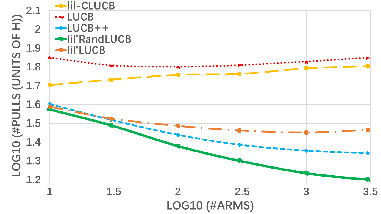
(a) (Faithful) 1-Sparse, $K=2$

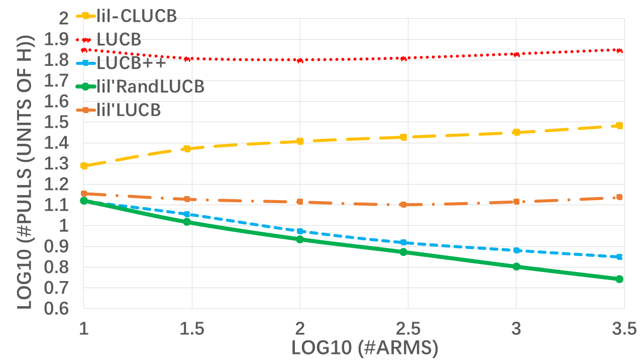
(b) (Heuristic) 1-Sparse, $K=2$

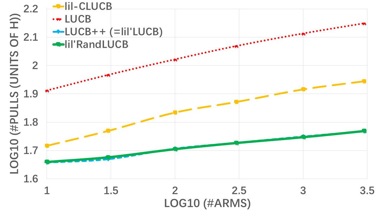
(c) (Faithful) 1-Sparse, $K=N/2$

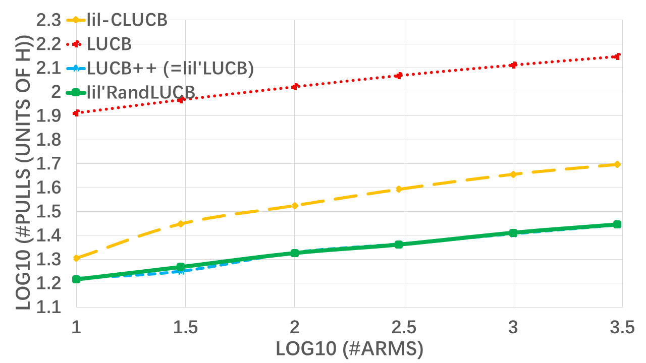
(d) (Heuristic) 1-Sparse, $K=N/2$

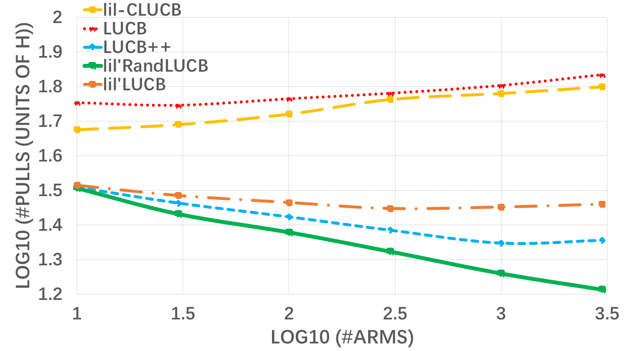
(e) (Faithful) 0.3-Exponential, $K=2$

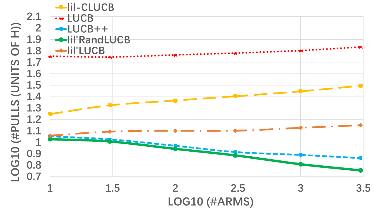
(f) (Heuristic) 0.3-Exponential, $K=2$

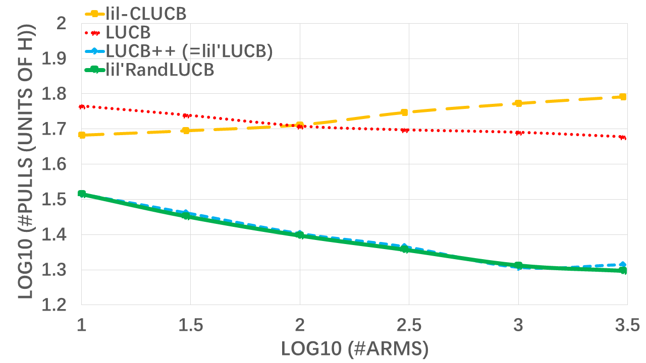
(g) (Faithful) 0.3-Exponential, $K=N/2$

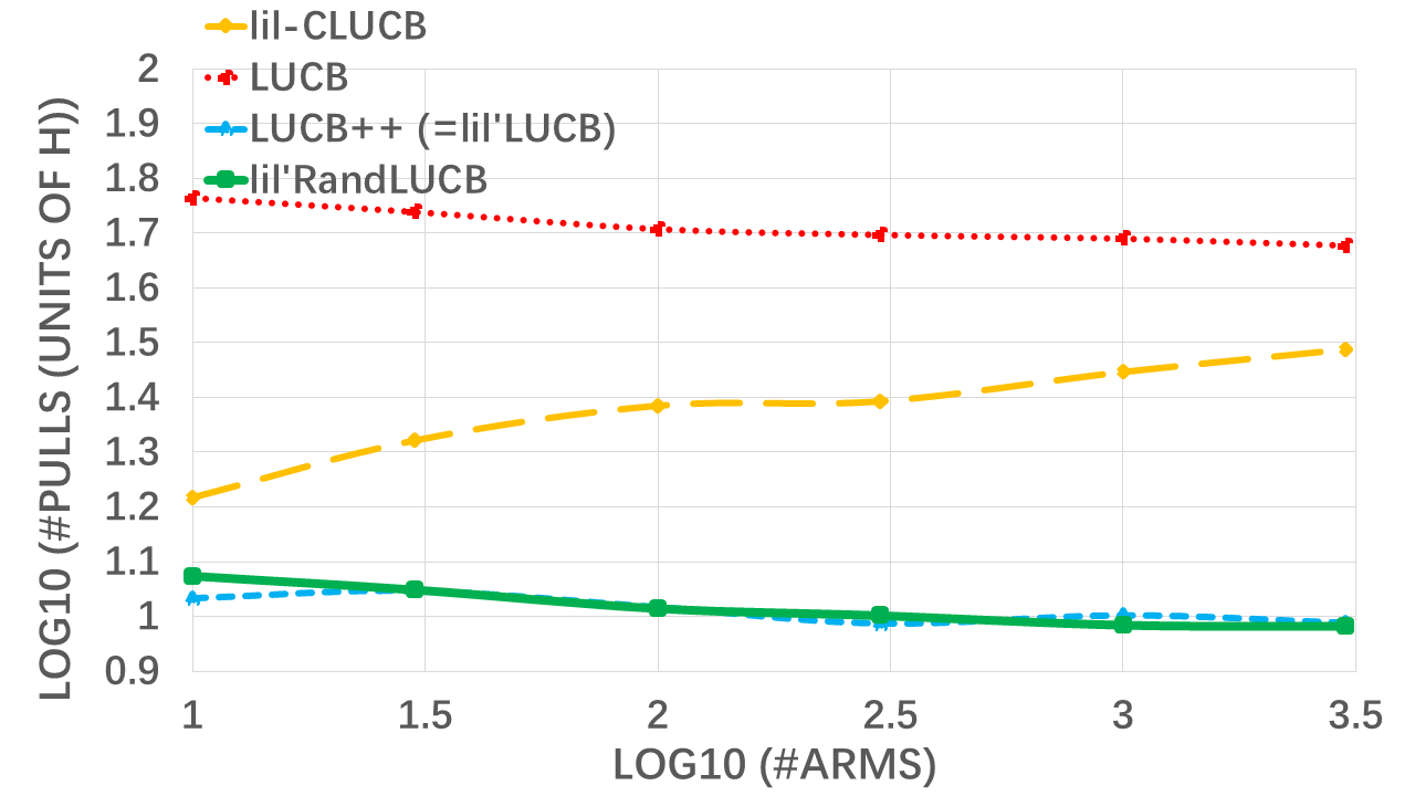
(h) (Heuristic) 0.3-Exponential, $K=N/2$

Figure 1: Results for Best-$K$-Arm, where $K=2$ or $K=N/2$.

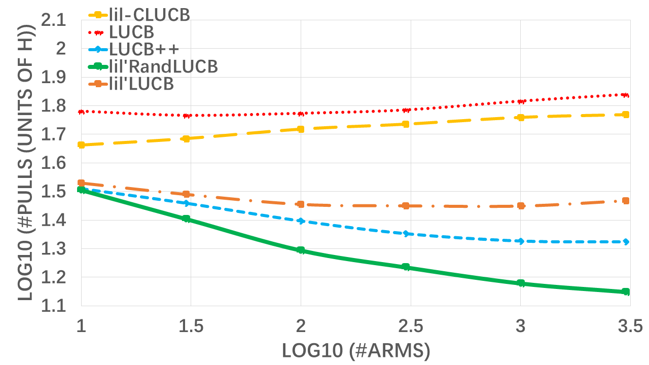
(a) (Faithful) 1-Sparse, K=1

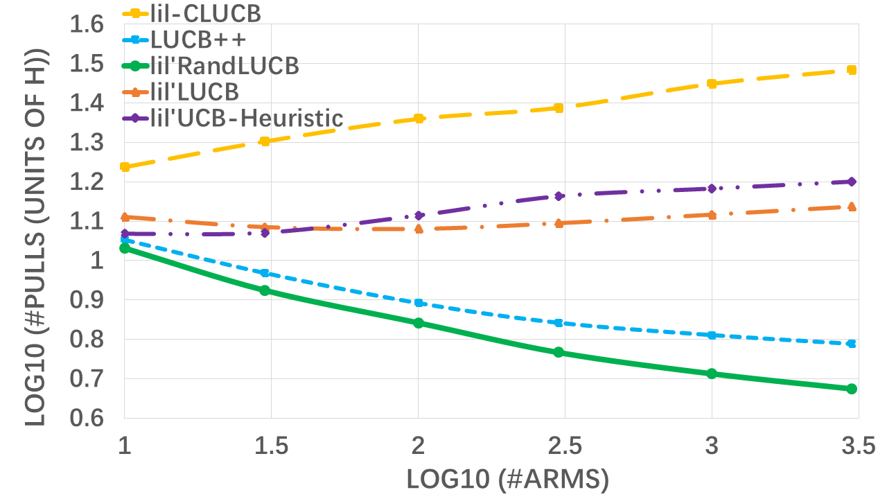
(b) (Heuristic) 1-Sparse, K=1

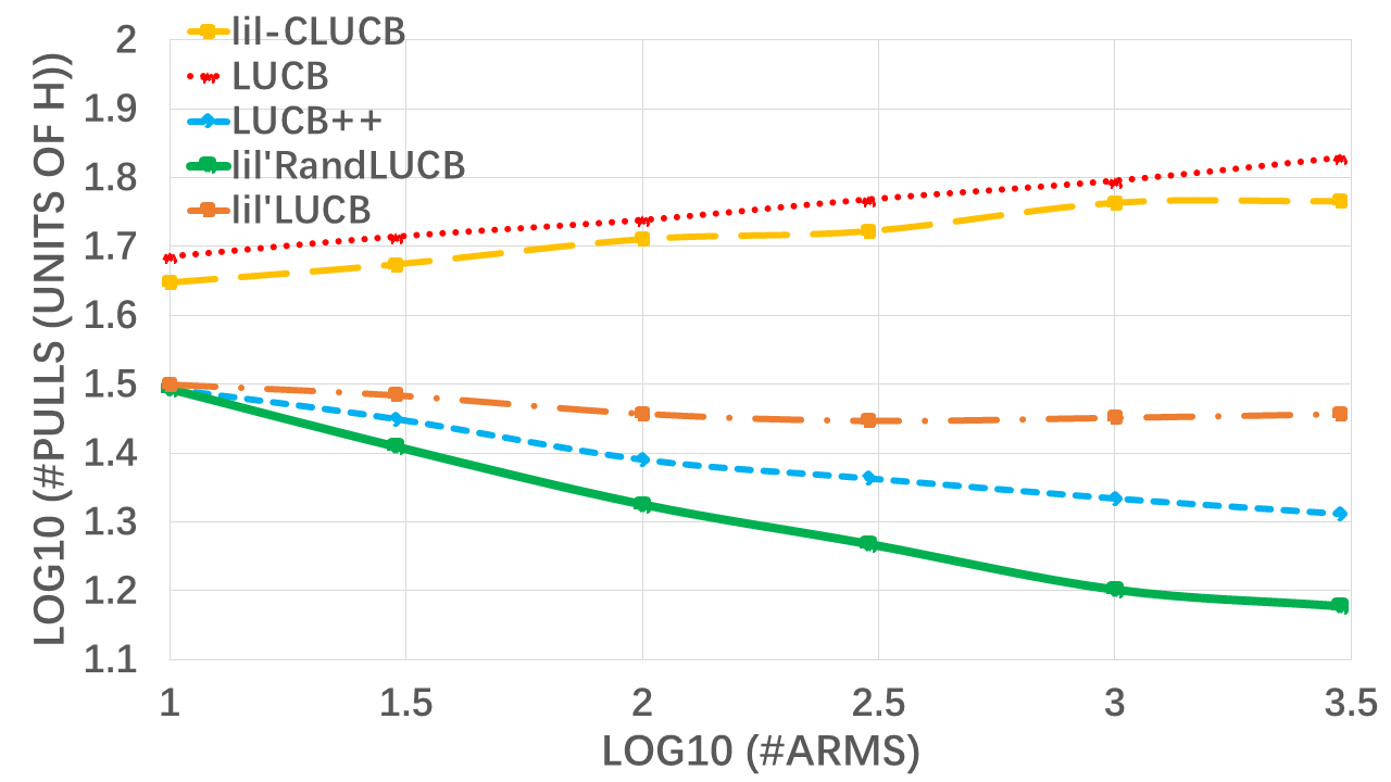
(c) (Faithful) $\alpha=0.3$, K=1

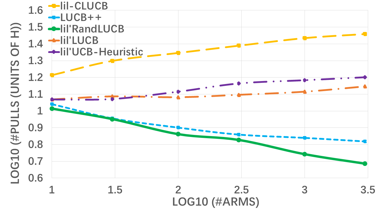
(d) (Heuristic) $\alpha=0.3$, K=1

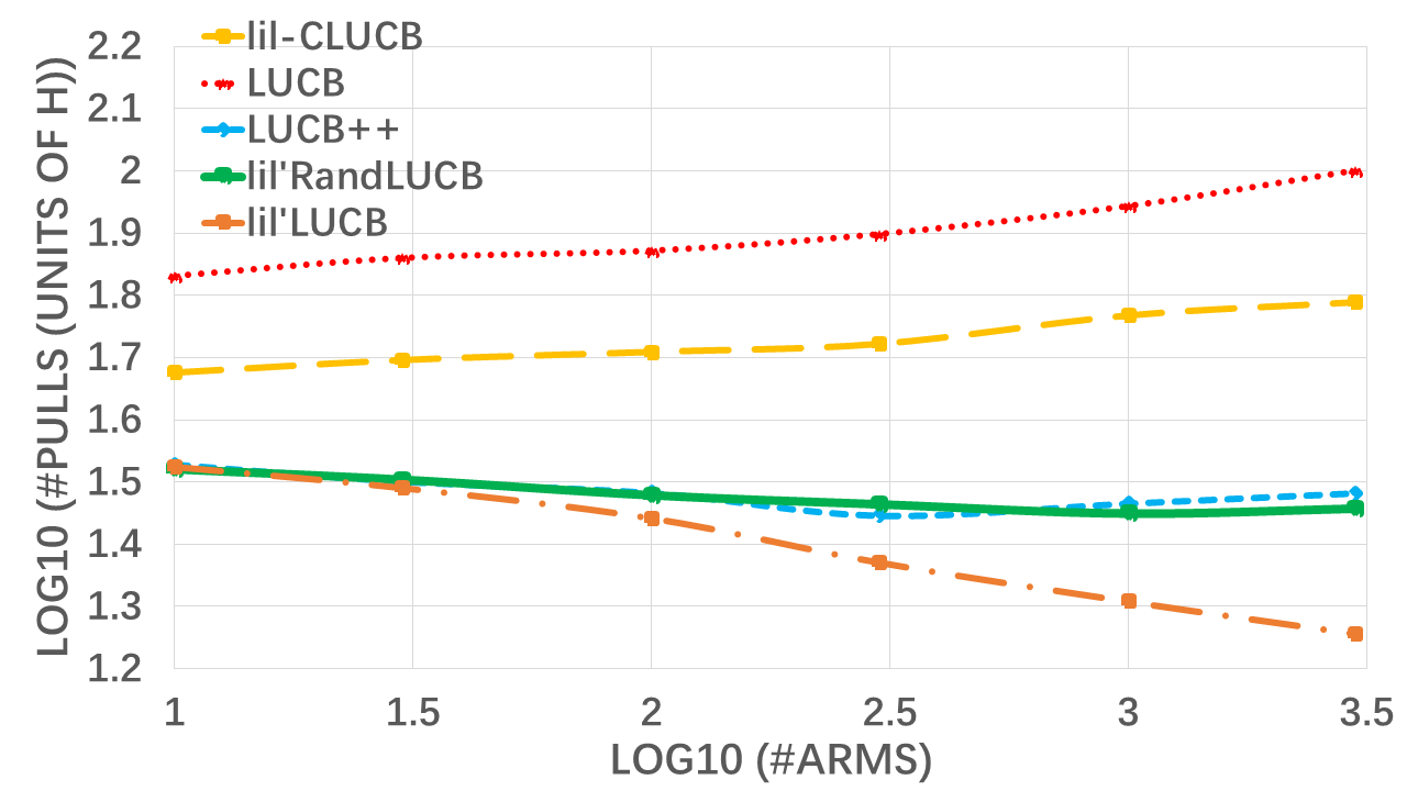
(e) (Faithful) $\alpha=0.6$, K=1

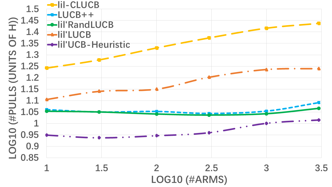
(f) (Heuristic) $\alpha=0.6$, K=1

Figure 2: Results for Best-1-Arm.

Appendix A A Technical Lemma

The following lemma follows from a direct calculation.

Lemma A.1.

For $t\geq 1,\epsilon\in(0,1),c>0,0<\omega\leq 1$,

$$\frac{1}{t}\log\Bigg{(}\frac{\log((1+\epsilon)t)}{\omega}\Bigg{)}\geq c\implies t\leq\frac{1}{c}\log\Bigg{(}\frac{2\log((1+\epsilon)/(c\omega))}{\omega}\large\Bigg{)}.$$

For $t\geq 1,s\geq 3,\epsilon\in(0,1],0<\omega\leq\delta\leq e^{-e}$,

$$\frac{1}{t}\log\Bigg{(}\frac{\log((1+\epsilon)t)}{\omega}\Bigg{)}\geq\frac{c}{s}\log\Bigg{(}\frac{\log((1+\epsilon)s)}{\delta}\Bigg{)}\implies t\leq\frac{s}{c}\cdot\frac{\log(2\log(\frac{1}{cw})/\omega)}{\log(1/\delta)}.$$

Appendix B Missing Proofs for lil’RandLUCB

In this section we present the missing proof of Theorem 3.1, which we restate below for convenience.

Theorem 3.1 (restated) With probability at least $1-c_{\epsilon}\delta$, lil’RandLUCB outputs the correct answer and takes

$$O\left(\sum_{i\in\mathcal{I}}\Delta_{i}^{-2}\left(\log\delta^{-1}+\log N+\log\log\Delta_{i}^{-1}\right)\right)$$

samples in expectation.

We start with the following simple lemma, which relates the difference between the means of two arms to their gaps.

Lemma B.1.

For any arm $i\in\mathrm{OPT}$ and arm $j\in\overline{\mathrm{OPT}}$, $\mu_{i}-\mu_{j}\geq(\Delta_{i}+\Delta_{j})/2$. For any two arms $i,j\in\mathrm{OPT}$, $\mu_{i}-\mu_{j}=\Delta_{i}-\Delta_{j}$.

Proof.

Recall that $\mu_{[t]}$ and $\Delta_{[t]}$ denote the mean and the gap of the $t$-th largest arm, respectively. Then for any $i\in\mathrm{OPT}$ and $j\in\overline{\mathrm{OPT}}$,

$$\mu_{i}-\mu_{j}=\Delta_{[i]}+\Delta_{[j]}-\Delta_{[K]}\geq\Delta_{[i]}+\Delta_{[j]}-(\Delta_{[i]}+\Delta_{[j]})/2=(\Delta_{[i]}+\Delta_{[j]})/2.$$

Moreover, for any $i,j\in\mathrm{OPT}$,

$$\mu_{i}-\mu_{j}=(\mu_{i}-\mu_{[K+1]})-(\mu_{j}-\mu_{[K+1]})=\Delta_{i}-\Delta_{j}.$$

∎

Now we prove Theorem 3.1.

Proof of Theorem 3.1.

We define $\mathcal{E}$ as the event that for all arm $i\in\mathrm{OPT}$ and integer $j\geq 1$, it holds that $\left|\widehat{\mu}_{i,j}-\mu_{i}\right|<U\left(j,\delta/(2K)\right)$. Moreover, for arm $i\in\overline{\mathrm{OPT}}$ and $j\geq 1$, $\left|\widehat{\mu}_{i,j}-\mu_{i}\right|<U\left(j,\delta/[2(N-K)]\right)$. By Lemma 2.1 and a union bound, event $\mathcal{E}$ happens with probability at least

$$1-K\cdot c_{\epsilon}\left(\delta/(2K)\right)^{1+\epsilon}-(N-K)\cdot c_{\epsilon}\left(\delta/[2(N-K)]\right)^{1+\epsilon}$$

$$\geq 1-K\cdot c_{\epsilon}\left(\delta/(2K)\right)-(N-K)\cdot c_{\epsilon}\left(\delta/[2(N-K)]\right)$$

$$\geq 1-c_{\epsilon}\delta.$$

It remains to prove the correctness and the sample complexity bound of lil’RandLUCB conditioning on event $\mathcal{E}$.

Conditional correctness.

Suppose for the purpose of contradiction the algorithm terminates at time $t$ and returns $\mathrm{High}_{t}\neq\mathrm{OPT}$. In this case, there exists $i\in\mathrm{High}_{t}\cap\overline{\mathrm{OPT}}$ and $j\in\mathrm{Low}_{t}\cap\mathrm{OPT}$. Recall that $h_{t}$ is the arm in $\mathrm{High}_{t}$ with the lowest lower confidence bound and $l_{t}$ is the arm in $\mathrm{Low}_{t}$ with the highest upper confidence bound. The definition of $h_{t}$ and event $\mathcal{E}$ guarantees that conditioning on $\mathcal{E}$,

$$\mu_{i}>\widehat{\mu}_{i,T_{i}(t)}-U\left(T_{i}(t),\delta/[2(N-K)]\right)\geq\widehat{\mu}_{h_{t},T_{h_{t}}(t)}-U\left(T_{h_{t}}(t),\delta/[2(N-K)]\right).$$

Similarly,

$$\mu_{j}<\widehat{\mu}_{j,T_{j}(t)}+U\left(T_{j}(t),\delta/(2K)\right)\leq\widehat{\mu}_{l_{t},T_{l_{t}}(t)}+U\left(T_{l_{t}}(t),\delta/(2K)\right).$$

The stopping condition at round $t$ implies that

$$\widehat{\mu}_{h_{t},T_{h_{t}}(t)}-U\left(T_{h_{t}}(t),\delta/[2(N-K)]\right)\geq\widehat{\mu}_{l_{t},T_{l_{t}}(t)}+U\left(T_{l_{t}}(t),\delta/(2K)\right).$$

The three inequalities above together yield $\mu_{i}>\mu_{j}$, which contradicts the assumption that $i\in\overline{\mathrm{OPT}}$ and $j\in\mathrm{OPT}$. Thus, lil’RandLUCB outputs the correct answer conditioning on event $\mathcal{E}$.

Sample complexity bound.

We upper bound the sample complexity of lil’RandLUCB by means of a charging argument. We define the critical arm at time $t$, denoted by $\mathrm{cr}_{t}$, as the arm that has been pulled fewer times between $h_{t}$ and $l_{t}$, i.e., $\mathrm{cr}_{t}=\operatorname*{argmin}_{i\in\{h_{t},l_{t}\}}T_{i}(t)$. We “charge” the critical arm a cost of $1$, no matter whether it is actually pulled at this time step. It remains to upper bound the total cost that we charge each arm. To this end, we prove the following two claims:

• Once an arm has been sampled a certain number of times, it will never be critical in the future.

• The expected number of samples drawn from an arm is lower bounded by the total cost it is charged.

This directly gives an upper bound on the cost that we charge each arm, and thus an upper bound on the total sample complexity.

First claim: no charging after enough samples.

For a fixed time step $t$, define $\widehat{\mu}_{i}=\widehat{\mu}_{i,T_{i}(t)}$ and $r_{i}=U\left(T_{i}(t),\delta/(2N)\right).$ Since $\delta/(2N)$ is smaller than $\delta/(2K)$ and $\delta/[2(N-K)]$, $r_{i}$ is greater than or equal to both $U(T_{i}(t),\delta/(2K))$ and $U(T_{i}(t),\delta/[2(N-K)]).$ It follows that conditioning on event $\mathcal{E}$, $|\widehat{\mu}_{i}-\mu_{i}|<r_{i}$ holds for every arm $i$.

In the following, we show that $r_{\mathrm{cr}_{t}}\geq\Delta_{\mathrm{cr}_{t}}/8$. In other words, let $\tau_{i}$ denote the smallest integer such that $U\left(\tau_{i},\delta/(2N)\right)<\Delta_{i}/8$. Then once arm $i$ has been sampled $\tau_{i}$ times, it will never become critical later.

We prove the inequality in the following three cases separately.

Case 1. $h_{t}\in\overline{\mathrm{OPT}}$, $l_{t}\in\mathrm{OPT}$. Since $h_{t}\in\mathrm{High}_{t}$ and $l_{t}\in\mathrm{Low}_{t}$, we have $\widehat{\mu}_{h_{t}}\geq\widehat{\mu}_{l_{t}}$. It follows that conditioning on event $\mathcal{E}$,

$$\mu_{h_{t}}+r_{h_{t}}>\widehat{\mu}_{h_{t}}\geq\widehat{\mu}_{l_{t}}>\mu_{l_{t}}-r_{l_{t}},$$

which implies that

$$r_{h_{t}}+r_{l_{t}}>\mu_{l_{t}}-\mu_{h_{t}}\geq(\Delta_{h_{t}}+\Delta_{l_{t}})/2.$$

The last step applies Lemma B.1. Recall that arm $\mathrm{cr}_{t}$ has been pulled fewer times than the other arm up to time $t$, and thus the arm has a larger confidence radius than the other arm. Then,

$$r_{\mathrm{cr}_{t}}\geq(r_{h_{t}}+r_{l_{t}})/2\geq(\Delta_{h_{t}}+\Delta_{l_{t}})/4\geq\Delta_{\mathrm{cr}_{t}}/4.$$

Case 2. $h_{t}\in\mathrm{OPT}$, $l_{t}\in\overline{\mathrm{OPT}}$. Since the stopping condition of lil’RandLUCB is not met, we have

$$\begin{split}\widehat{\mu}_{h_{t}}-r_{h_{t}}&\leq\widehat{\mu}_{h_{t}}-U\left(T_{h_{t}}(t),\delta/[2(N-K)]\right)\\ &<\widehat{\mu}_{l_{t}}+U\left(T_{l_{t}}(t),\delta/(2K)\right)\leq\widehat{\mu}_{l_{t}}+r_{l_{t}}.\end{split}$$

It follows that conditioning on $\mathcal{E}$,

$$\mu_{h_{t}}-2r_{h_{t}}<\widehat{\mu}_{h_{t}}-r_{h_{t}}<\widehat{\mu}_{l_{t}}+r_{l_{t}}<\mu_{l_{t}}+2r_{l_{t}},$$

which implies that, by Lemma B.1,

$$r_{h_{t}}+r_{l_{t}}>(\mu_{h_{t}}-\mu_{l_{t}})/2\geq(\Delta_{h_{t}}+\Delta_{l_{t}})/4.$$

Thus,

$$r_{\mathrm{cr}_{t}}\geq(r_{h_{t}}+r_{l_{t}})/2\geq(\Delta_{h_{t}}+\Delta_{l_{t}})/8\geq\Delta_{\mathrm{cr}_{t}}/8.$$

Case 3. $h_{t},l_{t}\in\mathrm{OPT}$ or $h_{t},l_{t}\in\overline{\mathrm{OPT}}$. By symmetry, it suffices to consider the former case. Since the arm $l_{t}$, which is among the best $K$ arms, is in $\mathrm{Low}_{t}$ by mistake, there must be another arm $j$ such that $j\in\overline{\mathrm{OPT}}\cap\mathrm{High}_{t}$. Recall that $h_{t}$ is the arm with the smallest lower confidence bound in $\mathrm{High}_{t}$. Thus we have

$$\begin{split}\mu_{h_{t}}-2r_{h_{t}}&<\widehat{\mu}_{h_{t}}-r_{h_{t}}\\ &\leq\widehat{\mu}_{h_{t}}-U\left(T_{h_{t}}(t),\delta/[2(N-K)]\right)\\ &\leq\widehat{\mu}_{j}-U\left(T_{j}(t),\delta/[2(N-K)]\right)<\mu_{j},\end{split}$$

and it follows from Lemma B.1 that

$$r_{h_{t}}>(\mu_{h_{t}}-\mu_{j})/2\geq(\Delta_{h_{t}}+\Delta_{j})/4\geq\Delta_{h_{t}}/4.$$ (1)

Thus, if $\mathrm{cr}_{t}=h_{t}$, the claim directly holds. It remains to consider the case $\mathrm{cr}_{t}=l_{t}$.

Since $\widehat{\mu}_{h_{t}}\geq\widehat{\mu}_{l_{t}}$, we have

$$\mu_{l_{t}}-r_{l_{t}}<\widehat{\mu}_{l_{t}}\leq\widehat{\mu}_{h_{t}}<\mu_{h_{t}}+r_{h_{t}},$$

and it follows from Lemma B.1 that

$$r_{h_{t}}+r_{l_{t}}>\mu_{l_{t}}-\mu_{h_{t}}=\Delta_{l_{t}}-\Delta_{h_{t}}.$$ (2)

Since we charge $\mathrm{cr}_{t}=l_{t}$, it holds that $r_{l_{t}}\geq r_{h_{t}}$, and thus by (1) and (2),

$$r_{l_{t}}\geq(r_{h_{t}}+r_{l_{t}})/6+2r_{h_{t}}/3>(\Delta_{l_{t}}-\Delta_{h_{t}})/6+\Delta_{h_{t}}/6=\Delta_{l_{t}}/6.$$

This finishes the proof of the claim.

Second claim: lower bound samples by costs.

We note that when we charge arm $\mathrm{cr}_{t}$ with a cost of $1$ at time step $t$, it holds that $T_{\mathrm{cr}_{t}}(t)\leq(T_{h_{t}}(t)+T_{l_{t}}(t))/2$. According to lil’RandLUCB, arm $\mathrm{cr}_{t}$ is pulled at time $t$ with probability at least $1/2$. Recall that $\tau_{i}$ is defined as the smallest integer such that $U(\tau_{i},\delta/(2N))<\Delta_{i}/8$. Let random variable $X_{i}$ denote that number of times that arm $i$ is charged before it has been pulled $\tau_{i}$ times. Since in expectation, an arm will get a sample after being charged at most twice, we have $\textbf{E}[X_{i}]\leq 2\tau_{i}$.

By Lemma A.1,

$$\tau_{i}=O\left(\Delta_{i}^{-2}\left(\log\delta^{-1}+\log N+\log\log\Delta_{i}^{-1}\right)\right).$$

Therefore, the sample complexity of the algorithm conditioning on event $\mathcal{E}$ is upper bounded by

$$\sum_{i\in\mathcal{I}}\textbf{E}[X_{i}]=O\left(\sum_{i\in\mathcal{I}}\tau_{i}\right)=O\left(\sum_{i\in\mathcal{I}}\Delta_{i}^{-2}\left(\log\delta^{-1}+\log N+\log\log\Delta_{i}^{-1}\right)\right).$$

∎

Appendix C lil’CLUCB Algorithm

In this section, we give a formal description of the lil’CLUCB algorithm. The algorithm is shown in Algorithm 2.

Initialization: Sample each arm once, and let $T_{i}(N)\leftarrow 1$ for each $i\in\mathcal{I}$;

for $t=N,N+1,...$ do

       $M_{t}\leftarrow$ $K$ arms with the highest empirical means;

       for $i\in\mathcal{I}$ do  $u_{i,T_{i}(t)}\leftarrow U(T_{i}(t),\delta/N)$ ;

       for $i\in M_{t}$ do  $\widetilde{\mu}_{i,T_{i}(t)}\leftarrow\widehat{\mu}_{i,T_{i}(t)}-u_{i,T_{i}(t)}$ ;

       for $i\in\mathcal{I}\setminus M_{t}$ do  $\widetilde{\mu}_{i,T_{i}(t)}\leftarrow\widehat{\mu}_{i,T_{i}(t)}+u_{i,T_{i}(t)}$ ;

       $\widetilde{M}_{t}$ $\leftarrow$ the $K$ arms with the largest mean with respect to $\widetilde{\mu}$;

       if $M_{t}=\widetilde{M_{t}}$ then return $M_{t}$;

       Sample $I_{t}\leftarrow\operatorname*{argmax}_{i\in M_{t}\bigtriangleup\widetilde{M_{t}}}u_{i,T_{i}(t)}$;

       for $i\in\mathcal{I}$ do  $T_{i}(t+1)\leftarrow T_{i}(t)+\mathbbm{1}\left\{i=I_{t}\right\}$ ;

      

end for

Algorithm 2 $\textsf{lil'CLUCB}(\mathcal{I},K,\delta)$

Appendix D Missing Proofs for lil’CLUCB

In this section we show the proof for Theorem 4.1. The theorem is a straightforward corollary of the following lemmas.

Lemma D.1 (Validity of Confidence Bound).

With probability at least $1-c_{\epsilon}\delta^{1+\epsilon}/N^{\epsilon}$, the confidence bound for each arm is valid, i.e., for each $i\in\mathcal{I}$ and every $t\in\mathbb{N}$, we have

$$|\mu_{i}-\widehat{\mu}_{i,T_{i}(t)}|<U(T_{i}(t),\delta/N).$$

We denote the event that confidence bounds for all arms are valid as $\mathcal{E}$. For the following, we always condition on the event $\mathcal{E}$. It is not hard to see that given $\mathcal{E}$ holds, the algorithm always outputs the optimal solution.

Lemma D.2 (Correctness).

Given that the event $\mathcal{E}$ holds, the algorithm always outputs the correct answer.

Proof.

Suppose that the algorithm terminates at time $t$. For the purpose of contradiction, we assume that the set $M_{t}$ is not the same as $\mathrm{OPT}$. Then there exists an arm $e\in M_{t}\setminus\mathrm{OPT}$, and an arm $e^{\prime}\in\mathrm{OPT}\setminus M_{t}$. Since $M_{t}=\widetilde{M_{t}}$, $e\in\widetilde{M_{t}}\setminus\mathrm{OPT}$, and $e^{\prime}\in\mathrm{OPT}\setminus\widetilde{M_{t}}$. So $\widetilde{\mu}_{e,T_{e}(t)}\geq\widetilde{\mu}_{e^{\prime},T_{e^{\prime}}(t)}$. But since $\mu_{e^{\prime}}>\mu_{e}$, and due to validity of confidence bound, we have that $\widetilde{\mu}_{e^{\prime},T_{e^{\prime}}(t)}=\widehat{\mu}_{e^{\prime},T_{e^{\prime}}(t)}+u_{e^{\prime},T_{e^{\prime}}(t)}>\mu_{e^{\prime}}>\mu_{e}>\widehat{\mu}_{e,T_{e}(t)}-u_{e,T_{e}(t)}=\widetilde{\mu}_{e,T_{e}(t)}$, which leads to a contradiction. Therefore, given $\mathcal{E}$ the algorithm always outputs the correct answer.
∎

Now we analyze the sample complexity of lil’CLUCB. The next lemma shows that whenever the confidence radius of an arm is sufficiently small, then that arm will not be further sampled.

Lemma D.3.

Given that the event $\mathcal{E}$ holds. For any arm $e\in\mathcal{I}$, suppose $u_{e,T_{e}(t)}<\Delta_{e}/4$ at time $t$, then arm $e$ will not be sampled in that round. Notice that this is equivalent to saying that arm $e$ will not be sampled again, since the confidence radius is independent of time.

Proof.

We prove this lemma by considering all possible cases seperately. Suppose arm $e$ is sampled at some time $t$, then by the sampling strategy, $e$ must be in the symmetric difference between $M_{t}$ and $\widetilde{M}_{t}$, i.e. $M_{t}\bigtriangleup\widetilde{M}_{t}$. For simplicity of notation, we use $u_{i}$ to denote the confidence radius of arm $i$ at that moment. Then, $u_{e}\geq u_{a},\forall a\in M_{t}\bigtriangleup\widetilde{M}_{t}$. For the purpose of contradiction, we assume that $u_{e,T_{e}(t)}<\Delta_{e}/4$. We show that for each of the four cases below, we can obtain a contradiction: (1) $e\in\mathrm{OPT}\wedge e\in M_{t}\setminus\widetilde{M}_{t}$, (2) $e\in\mathrm{OPT}\wedge e\in\widetilde{M}_{t}\setminus M_{t}$, (3) $e\notin\mathrm{OPT}\wedge e\in M_{t}\setminus\widetilde{M}_{t}$ and (4) $e\notin\mathrm{OPT}\wedge e\in\widetilde{M}_{t}\setminus M_{t}$.

Case (1): Suppose that $e\in\mathrm{OPT}\wedge e\in M_{t}\setminus\widetilde{M}_{t}$. Then there exists $e^{\prime}\in\widetilde{M}_{t}$, s.t. $e^{\prime}\notin\mathrm{OPT}$. If $e^{\prime}\in\widetilde{M}_{t}\setminus M_{t}$, then $\mu_{e^{\prime}}+2u_{e^{\prime}}\geq\widehat{\mu}_{e^{\prime}}+u_{e^{\prime}}\geq\widehat{\mu}_{e}-u_{e}\geq\mu_{e}-2u_{e}$. Therefore, $\Delta_{e}>4\mu_{e}\geq\mu_{e}-\mu_{e^{\prime}}\geq\Delta_{e}$, which is a contradiction. Therefore, $e^{\prime}\in\widetilde{M}_{t}\cap M_{t}$. But then $\mu_{e^{\prime}}\geq\widehat{\mu}_{e^{\prime}}-u_{e^{\prime}}\geq\widehat{\mu}_{e}-u_{e}\geq\mu_{e}-2u_{e}$, which again leads to a contradiction.

Case (2): Suppose that $e\in\mathrm{OPT}\wedge e\in\widetilde{M}_{t}\setminus M_{t}$. Then there exists $e^{\prime}\in M_{t}$, but $e^{\prime}\notin\mathrm{OPT}$. Then $\widehat{\mu}_{e^{\prime}}\geq\widehat{\mu}_{e}$. If $e^{\prime}\in M_{t}\setminus\widetilde{M}_{t}$, then $\mu_{e^{\prime}}+u_{e^{\prime}}\geq\mu_{e}-u_{e}$, which leads to $\Delta_{e}\leq\mu_{e}-\mu_{e^{\prime}}\leq 2u_{e}<\Delta_{e}$, which is a contradiction. Therefore, it must be the case that each arm in $M_{t}\setminus\widetilde{M}_{t}$ belongs to $\mathrm{OPT}$, and we pick one of such arms $e^{\prime\prime}$. Then $\mu_{e^{\prime}}\geq\widehat{\mu}_{e^{\prime}}-u_{e^{\prime}}\geq\widehat{\mu}_{e^{\prime\prime}}-u_{e^{\prime\prime}}\geq\widehat{\mu}_{e}-u_{e^{\prime\prime}}\geq\mu_{e}-u_{e}-u_{e^{\prime\prime}}$. But since $u_{e}\geq u_{e^{\prime\prime}}$, then the above inequality implies $2u_{e}\geq\mu_{e}-\mu_{e^{\prime}}$, which is a contradiction.

Case (3): Suppose that $e\notin\mathrm{OPT}\wedge e\in M_{t}\setminus\widetilde{M}_{t}$. If there exists $e^{\prime}\in\mathrm{OPT}$ and $e^{\prime}\in\widetilde{M}_{t}\setminus M_{t}$, then $\mu_{e}+u_{e}\geq\widehat{\mu}_{e}\geq\widehat{\mu}_{e^{\prime}}\geq\mu_{e^{\prime}}-u_{e^{\prime}}$. But $u_{e}\geq u_{e^{\prime}}$, and therefore leads to a contradiction. So it must be the case that each arm in $\widetilde{M}_{t}\setminus M_{t}$ does not belong to $\mathrm{OPT}$. Therefore, there exists an arm $e^{\prime}\in\mathrm{OPT}$ but $e^{\prime}\notin M_{t}\cup\widetilde{M}_{t}$, and an arm $e^{\prime\prime}\in\widetilde{M}_{t}\setminus M_{t}$ such that $e^{\prime\prime}\notin\mathrm{OPT}$. Thus $\mu_{e}+u_{e}+u_{e^{\prime\prime}}\geq\widehat{\mu}_{e}+u_{e^{\prime\prime}}\geq\widehat{\mu}_{e^{\prime\prime}}+u_{e^{\prime\prime}}\geq\widehat{\mu}_{e^{\prime}}+u_{e^{\prime}}\geq\mu_{e^{\prime}}$, which leads to a contradiction $2u_{e}\geq\Delta_{e}$.

Cases (4): Suppose that $e\notin\mathrm{OPT}\wedge e\in\widetilde{M}_{t}\setminus M_{t}$. Then there exists an arm $e^{\prime}\in\mathrm{OPT}$ that is not in $\widetilde{M}_{t}$. If $e^{\prime}\in M_{t}\setminus\widetilde{M}_{t}$, then by the construction of $\widetilde{M}_{t}$, we have that $\mu_{e}+2u_{e}\geq\widehat{\mu}_{e}+u_{e}\geq\widehat{\mu}_{e^{\prime}}-u_{e^{\prime}}\geq\mu_{e^{\prime}}-2u_{e^{\prime}}$. Since $u_{e}>u_{e^{\prime}}$, it follows that $\Delta_{e}\leq\mu_{e^{\prime}}-\mu_{e}\leq 4u_{e}<\Delta_{e}$, which is a contradiction. If $e^{\prime}\notin M_{t}$, then $\mu_{e}+2u_{e}\geq\widehat{\mu}_{e}+u_{e}\geq\widehat{\mu}_{e^{\prime}}+u_{e^{\prime}}\geq\mu_{e^{\prime}}$, which also leads to a contradiction.
∎

Using the preceding lemma, we can bound the number of samples taken by lil’CLUCB.

Lemma D.4 (Sample Complexity).

Given the event $\mathcal{E}$ holds, then for each arm $i$, the total number of samples taken from arm $i$ is bounded by

$$O\left(\Delta_{i}^{-2}\left(\log\delta^{-1}+\log N+\log\log\Delta_{i}^{-1}\right)\right).$$

Therefore, the sample complexity of lil’CLUCB is

$$O\left(\sum_{i\in\mathcal{I}}\Delta_{i}^{-2}\left(\log\delta^{-1}+\log N+\log\log\Delta_{i}^{-1}\right)\right).$$

Proof.

Let $T_{i}$ be the total number of samples obtained from arm $i$. By the proceding lemma and by putting all the constant factors together, there exists some constant $C_{1}$, such that for each arm $i\in\mathcal{I}$, such that the following inequality holds.

$$\sqrt{\frac{1}{T_{i}}\log(N\log(T_{i})/\delta)}\leq C_{1}\Delta_{i}$$

Solving for this inequality, we have that there exists some constant $C_{2}$ such that

$$T_{i}\leq\frac{C_{2}}{\Delta_{i}^{2}}\log(N\log(N/\Delta_{e}^{2}\delta)/\delta)=O\left(\Delta_{i}^{-2}\left(\log\delta^{-1}+\log N+\log\log\Delta_{i}^{-1}\right)\right).$$

The lemma follows by summing over all arms. ∎

Appendix E Generalization of lil’CLUCB

In this section, we give more details on the generalization of lil’CLUCB to the combinatorial pure exploration (CPE) setting. The description of our generalized lil’CLUCB is given in algorithm 3. lil’CLUCB differs from CLUCB in that it uses a time-independent confidence radius, which allows us to obtain a better sample complexity upper bound.

Initialization: sample each arm once, $T_{i}(N)\leftarrow 1$ for each $i\in\mathcal{I}$;

for $t=N,N+1,...$ do

       $\mathbf{\widehat{\mu}}\leftarrow$ the vector of empirical means for all arms;

       $M_{t}$ $\leftarrow$ Oracle($\widehat{\mu}$);

       for $i\in\mathcal{I}$ do  $u_{i,T_{i}(t)}\leftarrow U(T_{i}(t),\delta/N)$ ;

       for $i\in M_{t}$ do  $\widetilde{\mu}_{i,T_{i}(t)}\leftarrow\widehat{\mu}_{i,T_{i}(t)}-u_{i,T_{i}(t)}$ ;

       for $i\in\mathcal{I}\setminus M_{t}$ do  $\widetilde{\mu}_{i,T_{i}(t)}\leftarrow\widehat{\mu}_{i,T_{i}(t)}+u_{i,T_{i}(t)}$ ;

       $\widetilde{M}_{t}$ $\leftarrow$ Oracle($\widetilde{\mu}$);

       if $M_{t}=\widetilde{M_{t}}$ then  return $M_{t}$ ;

       Sample $I_{t}\leftarrow\operatorname*{argmax}_{i\in M_{t}\bigtriangleup\widetilde{M_{t}}}u_{i,T_{i}(t)}$;

       for $i\in\mathcal{I}$ do  $T_{i}(t+1)\leftarrow T_{i}(t)+\mathbbm{1}\left\{i=I_{t}\right\}$ for each $i\in\mathcal{I}$ ;

      

end for

Algorithm 3 (Generalized) $\textsf{lil'CLUCB}(\mathcal{I},K,\delta)$. Parameter: $\epsilon$

Now we give the proof for Theorem 4.2, which is restated below.

Theorem 4.2 (restated) Suppose the reward distribution of each arm is $\sigma$-sub-Gaussian. For any $\delta\in(0,1)$ and decision class $\mathcal{M}\subseteq 2^{[N]}$, with probability at least $1-c_{\epsilon}\delta^{1+\epsilon}/N^{\epsilon}$, lil’CLUCB outputs the correct answer and takes at most

$$O\left(0pt(\mathcal{M})^{2}\sigma^{2}\sum_{i\in\mathcal{I}}\Delta_{i}^{-2}\left(\log\delta^{-1}+\log N+\log\log\Delta_{i}^{-1}\right)\right)$$

samples.

Proof.

By Lemma 2.1 and the stopping condition of lil’CLUCB, lil’CLUCB outputs the correct answer with probability at least $1-c_{\epsilon}\delta^{1+\epsilon}/N^{\epsilon}$. By [CLK⁺14, Lemma 10], once the confidence radius of an arm $i$ is smaller than $\Delta_{i}/(30pt(\mathcal{M}))$, that arm will no longer be pulled. Combined with Lemma A.1, the total number of samples obtained from arm $i$ is at most

$$O\left(0pt\left(\mathcal{M}\right)^{2}\sigma^{2}\Delta_{i}^{-2}\left(\log\delta^{-1}+\log N+\log\log\Delta_{i}^{-1}\right)\right).$$

Summing up over all arms proves the theorem. ∎

References

- [AB10] Jean-Yves Audibert and Sébastien Bubeck. Best arm identification in multi-armed bandits. In COLT-23th Conference on Learning Theory-2010, pages 13–p, 2010.
- [ACBF02] Peter Auer, Nicolo Cesa-Bianchi, and Paul Fischer. Finite-time analysis of the multiarmed bandit problem. Machine learning, 47(2-3):235–256, 2002.
- [BCB+12] Sébastien Bubeck, Nicolo Cesa-Bianchi, et al. Regret analysis of stochastic and nonstochastic multi-armed bandit problems. Foundations and Trends® in Machine Learning, 5(1):1–122, 2012.
- [BWV13] Sébastien Bubeck, Tengyao Wang, and Nitin Viswanathan. Multiple identifications in multi-armed bandits. In International Conference on Machine Learning, pages 258–265, 2013.
- [CGL16] Lijie Chen, Anupam Gupta, and Jian Li. Pure exploration of multi-armed bandit under matroid constraints. In 29th Annual Conference on Learning Theory, pages 647–669, 2016.
- [CL15] Lijie Chen and Jian Li. On the optimal sample complexity for best arm identification. arXiv preprint arXiv:1511.03774, 2015.
- [CL16] Alexandra Carpentier and Andrea Locatelli. Tight (lower) bounds for the fixed budget best arm identification bandit problem. In 29th Annual Conference on Learning Theory, pages 590–604, 2016.
- [CLK+14] Shouyuan Chen, Tian Lin, Irwin King, Michael R Lyu, and Wei Chen. Combinatorial pure exploration of multi-armed bandits. In Advances in Neural Information Processing Systems, pages 379–387, 2014.
- [CLQ16] Lijie Chen, Jian Li, and Mingda Qiao. Towards instance optimal bounds for best arm identification. arXiv preprint arXiv:1608.06031, 2016.
- [CLQ17] Lijie Chen, Jian Li, and Mingda Qiao. Nearly instance optimal sample complexity bounds for top-k arm selection. In Artificial Intelligence and Statistics, pages 101–110, 2017.
- [CLTL15] Wei Cao, Jian Li, Yufei Tao, and Zhize Li. On top-k selection in multi-armed bandits and hidden bipartite graphs. In Advances in Neural Information Processing Systems, pages 1036–1044, 2015.
- [EDMM06] Eyal Even-Dar, Shie Mannor, and Yishay Mansour. Action elimination and stopping conditions for the multi-armed bandit and reinforcement learning problems. Journal of machine learning research, 7(Jun):1079–1105, 2006.
- [GGL12] Victor Gabillon, Mohammad Ghavamzadeh, and Alessandro Lazaric. Best arm identification: A unified approach to fixed budget and fixed confidence. In Advances in Neural Information Processing Systems, pages 3212–3220, 2012.
- [GGLB11] Victor Gabillon, Mohammad Ghavamzadeh, Alessandro Lazaric, and Sébastien Bubeck. Multi-bandit best arm identification. In Advances in Neural Information Processing Systems, pages 2222–2230, 2011.
- [GK16] Aurélien Garivier and Emilie Kaufmann. Optimal best arm identification with fixed confidence. In Conference on Learning Theory (COLT), 2016.
- [GLG+16] Victor Gabillon, Alessandro Lazaric, Mohammad Ghavamzadeh, Ronald Ortner, and Peter Bartlett. Improved learning complexity in combinatorial pure exploration bandits. In Proceedings of the 19th International Conference on Artificial Intelligence and Statistics, pages 1004–1012, 2016.
- [JMNB14] Kevin Jamieson, Matthew Malloy, Robert Nowak, and Sébastien Bubeck. lil’ucb: An optimal exploration algorithm for multi-armed bandits. In Proceedings of The 27th Conference on Learning Theory, pages 423–439, 2014.
- [JN14] Kevin Jamieson and Robert Nowak. Best-arm identification algorithms for multi-armed bandits in the fixed confidence setting. In Information Sciences and Systems (CISS), 2014 48th Annual Conference on, pages 1–6. IEEE, 2014.
- [KCG15] Emilie Kaufmann, Olivier Cappé, and Aurélien Garivier. On the complexity of best arm identification in multi-armed bandit models. The Journal of Machine Learning Research, 2015.
- [KK13] Emilie Kaufmann and Shivaram Kalyanakrishnan. Information complexity in bandit subset selection. In Conference on Learning Theory, pages 228–251, 2013.
- [KKS13] Zohar Karnin, Tomer Koren, and Oren Somekh. Almost optimal exploration in multi-armed bandits. In Proceedings of The 30th International Conference on Machine Learning, pages 1238–1246, 2013.
- [KS10] Shivaram Kalyanakrishnan and Peter Stone. Efficient selection of multiple bandit arms: Theory and practice. In Proceedings of the 27th International Conference on Machine Learning (ICML-10), pages 511–518, 2010.
- [KTAS12] Shivaram Kalyanakrishnan, Ambuj Tewari, Peter Auer, and Peter Stone. Pac subset selection in stochastic multi-armed bandits. In Proceedings of the 29th International Conference on Machine Learning (ICML-12), pages 655–662, 2012.
- [MT04] Shie Mannor and John N Tsitsiklis. The sample complexity of exploration in the multi-armed bandit problem. Journal of Machine Learning Research, 5(Jun):623–648, 2004.
- [SJR17] Max Simchowitz, Kevin Jamieson, and Benjamin Recht. The simulator: Understanding adaptive sampling in the moderate-confidence regime. arXiv preprint arXiv:1702.05186, 2017.
- [ZCL14] Yuan Zhou, Xi Chen, and Jian Li. Optimal pac multiple arm identification with applications to crowdsourcing. In Proceedings of The 31st International Conference on Machine Learning, pages 217–225, 2014.