Variation of field enhancement factor near the emitter tip

Abstract

The field enhancement factor at the emitter tip and its variation in a close neighbourhood determines the emitter current in a Fowler-Nordheim like formulation. For an axially symmetric emitter with a smooth tip, it is shown that the variation can be accounted by a $\cos{\tilde{\theta}}$ factor in appropriately defined normalized co-ordinates. This is shown analytically for a hemiellipsoidal emitter and confirmed numerically for other emitter shapes with locally quadratic tips.

I Introduction

The field of vacuum nanoelectronics involves field electron emitters with sharp tips having radius of curvature in the nanometer regime. Due to the high aspect ratio, such emitters can have a large field enhancement factor, $\gamma_{a}$, at the apex (tip). Several models have been studied to gain insight into the dependence of height ($h$) and apex radius of curvature ($R_{a}$) on $\gamma_{a}$ EV2002 ; forbes2003 ; podenok ; read ; roveri ; bonard ; smith . Of these, the hemiellipsoid and hyperboloid emitters are analytically tractable kos ; pogorelov while the floating sphere at plane potential has been studied extensively but its predictions ($\gamma_{a}\simeq h/R_{a}$) far exceed the known results for $\gamma_{a}$ especially for sharp emitters ZPCL ; forbes2016 . A much studied numerical model is a cylindrical post with a hemispherical top choice for which various fitting formulas for $\gamma_{a}$ exist. A straightforward estimate forbes2003 is $\gamma_{a}\simeq 0.7(h/R_{a})$ while more eleborate ones EV2002 ; forbes2003 ; podenok ; read ; bonard are expressed as $\gamma_{a}\simeq a(b+h/R_{a})^{\sigma}$ with $0.9<\sigma\leq 1$. The $h/R_{a}$ dependence of $\gamma_{a}$ can be expected for various other vertically placed emitter shapes, though there are very few concrete results.

While there is some understanding of the local field enhancement at the emitter apex, its variation in the neighbourhood of the tip is not as clear. For the hemisphere on a plane, $\gamma(\theta)=\gamma_{a}\cos\theta$, where $\gamma_{a}=3$ and the origin is the center of the (hemi)sphere. For the hemiellipsoid or the hyperboloid, the local field at the emitter surface is known, though a geometric formula analogous to the hemisphere (the $\cos\theta$ dependence) is not known to exist. A recent numerical study bertan on the hemiellipsoid using the Ansys-Maxwell software includes the variation of $\gamma$ with angle $\theta$ from the center of the ellipsoid. For a hemisphere on a cylindrical post with the origin at the center of the hemisphere, the variation with $\theta$ was reported to be quadratic podenok while another study read found a $\cos^{1/2}\theta$ factor to be appropriate. In both cases, the angle is measured from the centre of the sphere. For a conical emitter rounded at the apex, Spindt et al Spindt found the $\theta$ dependence (measured from the centre of curvature at the tip) to be small close to the apex though a later study Li shows a sharper variation for small $\theta$. Clearly, more studies are required to understand the variation of $\gamma$ close to the apex.

The importance of the apex and its immediate neighbourhood arises from the fact that for sharp emitters, the enhancement factor generally falls rapidly away from the apex even for a decrease in height by only $R_{a}$. As a result, the tunneling transmission coefficient can fall by several orders of magnitude rendering the rest of the emitter inconsequential. The emitter current can thus be expressed as

$$I=\int_{0}^{\rho_{max}}2\pi\rho\sqrt{1+(dz/d\rho)^{2}}J({\bf{r}})~{}d\rho$$ (1)

where ${\bf{r}}=(\rho,z)$ is a point on the emitter surface, $\rho=\sqrt{x^{2}+y^{2}}$ and $\rho_{max}$ is a cutoff set by accuracy requirements. Here $J({\bf{r}})$ is the local current density FN ; Nordheim ; murphy ; jensen2003 ; forbes_deane ; jap2014 on the emitter surface, calculated by taking into account the local field enhancement factor $\gamma({\bf{r}})$. The enhancement factor $\gamma({\bf{r}})$ around the apex thus holds the key in any field emission calculation.

In the following, we shall first study the field enhancement factor for the hemiellipsoid and cast it in a generalized form $\gamma=\gamma_{a}\cos{\tilde{\theta}}$ where $\tilde{\theta}$ is defined using normalized co-ordinates ($\tilde{\rho},\tilde{z}$). We shall then deal with locally quadratic emitter tips and show numerically that the enhancement factor variation is well described by this generalization.

II Field Enhancement for the Hemiellipsoid

The vertical hemiellipsoid on a grounded conducting plane placed in an external electrostatic field ($E_{0}\hat{z}$) pointing along the axial direction is one of few analytically solvable models that have helped in understanding local field enhancement. It is convenient to work in prolate spheroidal coordinate system ($\xi,\eta,\phi$). These are related to the Cartesian coordinates by the following relations:

$$x=L\sqrt{({\eta^{2}}-1)(1-{\xi^{2}})}\cos{\phi}$$

$$y=L\sqrt{({\eta^{2}}-1)(1-{\xi^{2}})}\sin{\phi}$$

$$z=L\xi\eta,$$ (2)

where $L=\sqrt{h^{2}-b^{2}}$, $h$ is the height and $b$ is the radius of the base of the hemiellipsoid respectively. Note that a surface obtained by fixing $\eta=\eta_{0}$ in this coordinate system is an ellipsoid. For a prolate hemiellipsoid on a grounded plane in the presence of an external electrostatic field $-E_{0}\hat{z}$, the solution of Laplace equation may be written askos ; jap2016 ,

$$V(\eta,\xi)=\xi\eta\left[C^{\prime}+D^{\prime}\left({\frac{1}{2}}\ln{\frac{\eta+1}{\eta-1}}-{\frac{1}{\eta}}\right)\right],$$ (3)

where $C^{\prime}=LE_{0}$ and

$$D^{\prime}=-LE_{0}\left({\frac{1}{2}}\ln{\frac{\eta_{0}+1}{\eta_{0}-1}}-{\frac{1}{\eta_{0}}}\right)^{-1}$$ (4)

where $\eta=\eta_{0}$ is the surface of the emitter.

In order to relate this to the enhancement factor, $\gamma$, we need to find the normal derivative of the potential, $V$ at the surface of the emitter. To do so, we first note that

$${\bf E}_{local}=-\hat{\eta}\left[{\frac{1}{h_{\eta}}}{\frac{\partial V}{\partial\eta}}\right]_{\eta=\eta_{0}}$$ (5)

where

$$h_{\eta}=\sqrt{\frac{L^{2}}{\eta_{0}^{2}-1}(\eta_{0}^{2}-\xi^{2})}.$$ (6)

The magnitude of the local electric field normal to the surface $\eta=\eta_{0}$ is thus given by

$$E_{local}=-{\frac{\xi}{h_{\eta}}}\left[C^{\prime}+{\frac{D^{\prime}}{2}}\ln{\frac{\eta_{0}+1}{\eta_{0}-1}}-{\frac{D^{\prime}\eta_{0}}{\eta_{0}^{2}-1}}\right]$$ (7)

Note that at the apex of the hemiellipsoid $\xi=1$. Thus

$$\frac{\gamma}{\gamma_{a}}=\frac{\xi\sqrt{\eta_{0}^{2}-1}}{\sqrt{\eta_{0}^{2}-\xi^{2}}}$$ (8)

Further, with $\xi=z/h$, $L^{2}=h^{2}-b^{2}$, $R_{a}=b^{2}/h$ and $z^{2}/h^{2}+\rho^{2}/b^{2}=1$, we have

$$\gamma=\gamma_{a}\xi\sqrt{\frac{b^{2}}{\frac{b^{2}}{h^{2}}z^{2}+h^{2}-z^{2}}}$$ (9)

so that

$$\gamma=\gamma_{a}\xi\sqrt{\frac{b^{2}}{\frac{b^{2}}{h^{2}}z^{2}+\frac{h^{2}}{b^{2}}\rho^{2}}}$$ (10)

and finally

$$\gamma=\gamma_{a}\frac{z/h}{\sqrt{(z/h)^{2}+(\rho/R_{a})^{2}}}.$$ (11)

With $\tilde{z}=z/h$ and $\tilde{\rho}=\rho/R_{a}$, we define

$$\cos\tilde{\theta}=\frac{\tilde{z}}{\sqrt{{\tilde{z}}^{2}+{\tilde{\rho}}^{2}}}$$ (12)

so that $\gamma=\gamma_{a}\cos\tilde{\theta}$. In the limit of the hemisphere where $h=R=R_{a}$, $\tilde{\theta}=\theta$. Thus, both the hemiellipsoid and hemisphere can be described by Eq. 11.

III Quadratic surfaces

Generic smooth axially symmetric vertical emitter tips can be described as $z=z(\rho)$. A Taylor expansion at the apex yields

$$z = h+\frac{1}{2}\Big{(}\frac{d^{2}z}{d\rho^{2}}\Big{)}_{\rho=0}\rho^{2}+\ldots$$ (13)

$$\simeq h\Big{[}1-\frac{1}{2}\frac{\rho}{R_{a}}\frac{\rho}{h}\Big{]}$$ (14)

where $R_{a}$ is the magnitude of the apex radius of curvature and $h$ is the height of the emitter. We have assumed that the quadratic term is non-zero since $(d^{2}z/d\rho^{2})_{\rho=0}=0$ implies that the tip is flat rather than having a small radius of curvature characteristic of field emitters. Also, since field emission occurs close to the tip, we shall ignore higher order terms in $\rho$ as in Eq. 14.

The ellipsoid for instance can be expanded as

$$z=h\Big{[}1-\frac{1}{2}\frac{\rho}{R_{a}}\frac{\rho}{h}-\frac{1}{8}\Big{(}\frac{\rho}{R_{a}}\Big{)}^{2}\Big{(}\frac{\rho}{h}\Big{)}^{2}-\frac{1}{16}\Big{(}\frac{\rho}{R_{a}}\Big{)}^{3}\Big{(}\frac{\rho}{h}\Big{)}^{3}-\ldots\Big{]}$$ (15)

which reduces to

$$z=R\Big{[}1-\frac{1}{2}\Big{(}\frac{\rho}{R}\Big{)}^{2}-\frac{1}{8}\Big{(}\frac{\rho}{R}\Big{)}^{4}-\frac{1}{16}\Big{(}\frac{\rho}{R}\Big{)}^{6}-\ldots\Big{]}$$ (16)

for the sphere. For hemiellipsoidal emitters with large $h$, a quadratic truncation seems adequate.

Such quadratic emitter tips can thus be considered generic for purposes of field emission. They may be mounted on a variety of bases, ranging from the classical cylindrical post typical of carbon nanotubes to the conical bases of a Spindt array Spindt or even be part of compound structures. We shall study the applicability of Eq. 11 for such emitter tips numerically.

IV Numerical Studies

We shall adopt the nonlinear line charge model jap2016 ; harris_inf3 to determine the electrostatic potential and thus the field enhancement factor. It consists of a vertically placed line charge of height ${\cal L}$ on a grounded plane in the presence of an external electrostatic field $E_{0}$. The line charge together with its image and the external field produces a zero-potential surface that coincides with the emitter surface under study. The shape of the zero-potential surface crucially depends on the line charge density. Thus for a linear line charge density the shapes generated are hemiellipsoidal, while non-linear line charge densities can generate a wide variety of shapes including a conical base with a quadratic top.

For our purposes, we consider a polynomial line charge density $\Lambda(z)=\sum_{n=0}^{N}c_{n}z^{n}$ with the coefficients $c_{n}$ chosen appropriately. The potential at a point external to the emitter can thus be expressed as

$$V(x,y,z) = \frac{1}{4\pi\epsilon_{0}}\Big{[}\int_{0}^{L}ds\frac{\Lambda(s)}{(\rho^{2}+(z-s)^{2})^{1/2}}$$

$$- \int_{0}^{L}ds\frac{\Lambda(s)}{(\rho^{2}+(z+s)^{2})^{1/2}}\Big{]}-E_{0}z$$

where $\rho^{2}=x^{2}+y^{2}$. The local electrostatic field, ${\bf{E}}=-\nabla(V)$, can thus be used to determine the field enhancement factor $\gamma$ on the surface of the emitter. We have validated the method successfully using the hemiellipsoidal emitter over a range of aspect ratios. We have chosen a variety of emitter shapes for our study with parameters values that allow a span of the apex enhancement factor from a few 100s to 12000.

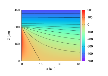
Figure 1: A contour plot of the potential for a grounded conical emitter of height $h=300~{}\mu$m and base radius $b=16~{}\mu$m in an external electrostatic field $E_{0}=1$ MV/m.

Figure 2: The conical tip is rounded due to the nature of the line charge distribution. The apex radius of curvature $R_{a}=4.56$ nm in this case. A quadratic $z=h-a\rho^{2}$ (solid line) fits well in the neighbourhood of the tip.

Fig. 1 shows the potential profile of a single circular cone-shaped emitter on an infinite grounded metallic plate, placed in an external field ${\bf{E}}=\hat{z}E_{0}$ where $E_{0}=1$ MV/m. The height of the cone is $300~{}\mu$m while the base radius $b=16~{}\mu$m. The line charge density is such that the tip is rounded at the apex. The zero contour profile near the tip is shown in Fig. 2 along with a quadratic fit $z=h-a_{2}\rho^{2}$ with $a_{2}=109.65~{}\mu{\rm m}^{-1}$. The excellent agreement shows that the region near the tip is locally a quadratic surface, with the apex radius of curvature $R_{a}=1/(2a_{2})\simeq 4.56$ nm. The variation of the enhancement factor $\gamma(z)$ near the apex is shown in Fig. 3. along with the curve $\gamma_{a}\cos\tilde{\theta}$ (see Eq. 11), calculated using the height $h$ and the apex radius of curvature $R_{a}$. The agreement shows that, close to the apex, the variation in the field enhancement factor is well described by the formula derived for an hemiellipsoid.

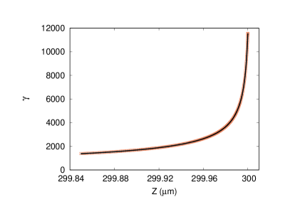
Figure 3: The variation of the enhancement factor $\gamma$ near the tip of the cone is compared with $\gamma_{a}\cos\tilde{\theta}$.

We next consider 2 surfaces of height $1500~{}\mu$m and base radius $b=20~{}\mu$m with a quadratic tops. In the first case, the apex radius of curvature $R_{a}=0.77~{}\mu$m while for the second $R_{a}=1.18~{}\mu$m. The apex enhancement factor are $\gamma_{a}=571$ and $\gamma_{a}=402$ respectively. The variation of the enhancement factor $\gamma$ is shown in Fig. 4. In both cases, Eq. 11 describes the variation well.

As a final example, we consider a cylindrical post with a top that is locally quadratic, typical of carbon nanotubes. The height of the system is $101~{}\mu$m while the base radius is $1~{}\mu$m. The potential profile in the presence of an external electrostatic field $E_{0}=1$ MV/m, is shown in Fig. 5. The apex radius of curvature $R_{a}=0.1278~{}\mu$m. Fig. 6 shows the variation of the enhancement factor $\gamma$. As before, Eq. 11 describes the variation in enhancement factor very well.

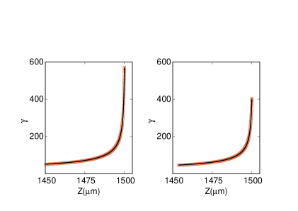
Figure 4: The variation of the enhancement factor $\gamma$ near the tip of 2 surfaces of height 1500 $\mu$m and base radius 20 $\mu$m, having apex radius of curvature 0.77 $\mu$m (left) and 1.18 $\mu$m (right). Their apex enhancement factors (the value of $\gamma$ at $z=1500~{}\mu$m) are 571 and 402 respectively. For both cases, Eq. 11 is also plotted (solid lines) and found to describe the variation well.

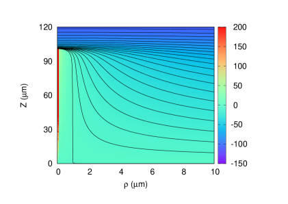
Figure 5: A contour plot of the potential for a grounded emitter shaped as a cylindrical post with a generic top. The total height $h=101~{}\mu$m while the base radius $b=1~{}\mu$m and the external electrostatic field $E_{0}=1$ MV/m. The apex enhancement factor $\gamma_{a}=285$.

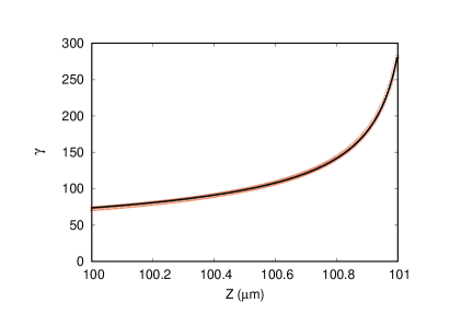
Figure 6: The variation of the enhancement factor $\gamma$ near the tip for the cylindrical post with a locally quadratic non-spherical top. The apex enhancement factor is 285. The solid line is Eq. 11 with $h=101~{}\mu$m and $R_{a}=0.1278~{}\mu$m.

The variation in field enhancement factor expressed in Eq. 11 is thus found to hold for a variety of shapes apart from the hemiellipsoid for which it was derived. We have tested its veracity for numerous other shapes that have not been presented here, including compound shapes formed by mounting an emitter on a pedestral such as a cylinder.

V Discussion and Conclusion

Before summarizing our results, we make a couple of observations. First, we believe the results presented here to be generic and hence applicable to a wide class of emitters provided the anode is flat and the anode-cathode gap large compared to the height of the emitter. There is however a discrepancy with the numerical results reported for the hemisphere on a cylindrical post podenok ; read ; roveri where the surface variation of $\gamma$ seems to differ from Eq. 11 and appears to be qualitatively closer to the numerical result presented in Fig. 4 of [13] for a hemiellipsoid ellip ; notdone . It may also be noted that result of Dyke et al dyke53 for a cone with a spherical top does not fall within the ambit of the present work since the anode in their work dyke53 belongs to the same family as the cathode.

Second, a somewhat related problem is the distribution of excess charge on the surface of a conductor and its relation to the local curvature of the conductor. In the absence of an external field, the surface charge density $\sigma\sim\kappa_{G}^{1/4}$ for quadratic surfaces (such as an ellipsoid, paraboloid or a hyperboloid) where $\kappa_{G}$ is the local Gaussian curvature gaussian . For an ellipsoid,

$$\kappa_{G}=\frac{1}{R_{a}^{2}}\frac{1}{\big{[}(z/h)^{2}+(\rho/R_{a})^{2}\big{]}^{2}}$$ (18)

so that

$$\sigma\sim\frac{1}{\sqrt{(z/h)^{2}+(\rho/R_{a})^{2}}}.$$ (19)

For $z\sim h$, this is similar to Eq. 11 which describes the local field variation on the surface of a conductor, though in the presence of an external field ${\bf{E}}=-\hat{z}E_{0}$.

In conclusion, we have studied the variation in the field enhancement factor on the surface of a conductor close to it apex, in the presence of an external electrostatic field along the symmetry axis ($\hat{z}$). For the hemiellipsoid, we have expressed the variation exactly over the entire surface as a generalized $\cos\tilde{\theta}$ factor, similar to the hemisphere on a conducting plane. We have numerically tested the validity of the $\cos\tilde{\theta}$ factor extensively for other emitter shapes and found it to describe the variation effectively near the apex. Since the enhancement factor falls sharply away from the apex, such a description is adequate for purposes of field emission. Thus, a simplified description of emitters consists of tips that can be expressed as $z=h-\frac{1}{2R_{a}}\rho^{2}$, where both the height $h$ and apex radius $R_{a}$ are experimentally measurable parameters which can in turn be used to predict the field enhancement variation.

 

VI References

References

- (1) C. J. Edgcombe and U. Valdre, Phil. Mag. B 82, 987 (2002).
- (2) R. G. Forbes, C.J. Edgcombe and U. Valdrè, Ultramicroscopy 95, 65 (2003).
- (3) S. Podenok, M. Sveningsson, K. Hansen and E.E.B. Campbell, Nano 1, 87 (2006).
- (4) F. H. Read and N. J. Bowring, Nucl. Ins. Meth. Phys. Res. 519, 305 (2004).
- (5) D. S. Roveri, G. M. Sant’Anna, H. H. Bertan, J. F. Mologni, M. A. R. Alves and E. S. Braga, Ultramicroscopy, 160, 247 (2016).
- (6) J-M. Bonard, K. A. Dean, B. F. Coll and C. Klinke, Phys. Rev. Lett. 89, 197602 (2002).
- (7) R. C. Smith and S. R. P. Silva, J. App. Phys. 106, 014314 (2009).
- (8) H. G. Kosmahl, IEEE Trans. Electron Devices 38, 1534,1991.
- (9) E. G. Pogorelov, A. I. Zhbanov and Y.-C. Chang, Ultramicroscopy 109, 373 (2009).
- (10) A. I. Zhbanov, E. G. Pogorelov, Y.-C. Chang, and Y.-G. Lee, J. Appl. Phys. 110, 114311 (2011).
- (11) R. G. Forbes, J. App. Phys. 120, 054302 (2016).
- (12) The cylindrical post with a hemispherical top has been the model of choice for studying nanotubes bonard ; smith though differently shaped emitter tips mounted on a cylinderical post are perhaps more appropriate.
- (13) H. H. Bertan, D. S. Roveri, G. M. Sant’Anna, J. F. Mologni, E. S. Braga and M. A. R. Alves, Journal of Electrostatics, 81, 59 (2016).
- (14) C. A. Spindt, I. Brodie, L. Humphrey, and E. R. Westerberg, J. Appl. Phys. 47, 5248 (1976).
- (15) N. Li and B. Zeng, 25th International Vacuum Nanoelectronics Conference, Jeju, 2012, pp. 1-2. doi: 10.1109/IVNC.2012.6316885
- (16) R. H. Fowler and L. Nordheim, Proc. R. Soc. A 119, 173 (1928).
- (17) L. Nordheim, Proc. R. Soc. A 121, 626 (1928);
- (18) E. L. Murphy and R. H. Good, Phys. Rev. 102, 1464 (1956).
- (19) K. L. Jensen J. Vac. Sci. Technol. B, 21, 1528 (2003).
- (20) R. G. Forbes and J. H. B. Deane, Proc. Roy. Soc. A 463, 2907 (2007).
- (21) D. Biswas and R. Kumar,J. App. Phys. 115, 114302 (2014).
- (22) D. Biswas, G. Singh and R. Kumar, J. App. Phys. 120, 124307 (2016).
- (23) J. R. Harris, K. L. Jensen and D. A. Shiffler, J. Phys. D, 48, 385203 (2015).
- (24) A hemiellipsoid should follow Eq. 11 exactly provided the anode is flat and sufficiently far away from the cathode. We have verified this numerically as well using the line charge model. The results in [13] (in particular Fig. 4) for the ellipsoid therefore seems to be an aberration.
- (25) We have not been able generate to suitable nonlinear line charge density to model a cylindrical post with an exact hemispherical top.
- (26) W. P. Dyke, J. K. Trolan, W. W. Dolan, and G. Barnes, J. Appl. Phys. 34, 570 (1953).
- (27) See for example, D. J. Cross, J. Math. Phys. 55, 123504 (2014) or K. Bhattacharya, Phys. Scr. 91, 035501 (2016).