TTP17-026
The $n_{f}^{2}$ contributions to fermionic
four-loop form factors

Abstract

We compute the four-loop contributions to the photon quark and Higgs quark form factors involving two closed fermion loops. We present analytical results for all non-planar master integrals of the two non-planar integral families which enter our calculation.

PACS numbers: 11.15.Bt, 12.38.Bx, 12.38.Cy

1 Introduction

There are various aspects of form factors which promote them to important objects in any quantum field theory. In the framework of QCD form factors constitute building blocks for various production and decay processes, most prominently for Higgs boson production and the Drell-Yan process. Furthermore, form factors are the simplest Green’s functions with a non-trivial infrared structure which makes them ideal objects to investigate general infrared properties of gauge theories [1, 2, 3, 4, 5, 6, 7].

The main objects of this work are massless fermionic form factors where the fermions couple via a vector and scalar coupling to an external current. In the framework of the Standard Model they can be interpreted as photon quark and Higgs quark form factors. In the following we provide brief definitions of these objects.

The quark-antiquark-photon form factor is conveniently obtained from the photon quark vertex function $\Gamma^{\mu}_{q}$ by applying an appropriate projector. In $d=4-2\epsilon$ space-time dimensions we have

$$F_{q}(q^{2}) = -\frac{1}{4(1-\epsilon)q^{2}}\mbox{Tr}\left(q_{2}\!\!\!\!\!/\,\,\,\Gamma^{\mu}_{q}\,q_{1}\!\!\!\!\!/\,\,\,\gamma_{\mu}\right)\,,$$ (1)

with $q=q_{1}+q_{2}$. $q_{1}$ and $q_{2}$ are the incoming quark and antiquark momenta and $q$ is the momentum of the photon.

In analogy, the Higgs quark form factor is constructed from the Higgs quark vertex function $\Gamma_{q}$. For definiteness we consider in the following the coupling to bottom quarks and write

$$F_{b}(q^{2}) = -\frac{1}{2q^{2}}\mbox{Tr}\left(q_{2}\!\!\!\!\!/\,\,\,\Gamma_{b}\,q_{1}\!\!\!\!\!/\,\,\,\right)\,.$$ (2)

Sample Feynman diagrams contributing to $F_{q}$ and $F_{b}$ are shown in Fig. 1.

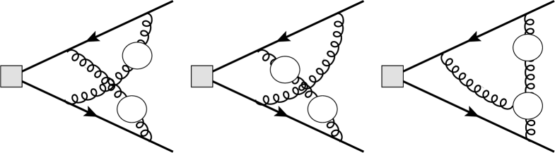
Figure 1: Sample Feynman diagrams contributing to $F_{q}$ and $F_{b}$ at the four-loop order and containing two closed fermion loops. The gray box indicates either a scalar or a vector coupling of the fermions to the external current. Solid and curly lines represent quarks and gluons, respectively. All particles are massless.

Two- and three-loop corrections to $F_{q}$ have been computed in Refs. [8, 9, 10, 11, 12, 13, 14, 15] and $F_{b}$ has been considered in Refs. [16, 17]. Four-loop results for $F_{q}$ in the planar limit have been obtained in Refs. [18, 19] and fermionic corrections with three closed quark loops have been computed in Ref. [20].

In this paper we consider fermionic contributions to $F_{q}$ and $F_{b}$. More precisely, we compute four-loop corrections with two closed fermion loops (which in our notation are proportional to $n_{f}^{2}$). This is the simplest well-defined gauge invariant subset which involves non-planar integral families. It is the main result of this work to study in detail these families and provide analytic results for all non-planar master integrals which are part of these families. Note, that all planar families including all master integrals have been considered in a systematic way in Refs. [18, 19, 21]. Non-planar integral families are already present in the $n_{f}^{3}$ contribution to the Higgs gluon form factor which has been considered in Ref. [20]. Very recently the $1/\epsilon^{2}$ pole of the four-loop form factor within ${\cal N}=4$ super Yang-Mills theory has been computed using numerical methods [22].

If $\epsilon^{0}$ terms at four loops shall be computed the lower-order corrections need to be expanded to higher orders in $\epsilon$. In particular, the one-, two- and three-loop results are needed to order $\epsilon^{6}$, $\epsilon^{4}$ and $\epsilon^{2}$, respectively. The three-loop $\epsilon^{2}$ terms for $F_{q}$ have been computed in Ref. [13] and cross-checked in Ref. [19]. As a preparatory calculation for the results obtained in this work we could confirm the three-loop corrections to the gluonic from factor up to order $\epsilon^{2}$ as given in Ref. [13]. Furthermore, we provide the first independent check for the three-loop $\epsilon^{0}$ term of $F_{b}$ [17] and extend it to order $\epsilon^{2}$ which is not yet available in the literature.

It is convenient to parametrize the form factor in terms of the bare strong coupling constant and write

$$F_{q} = 1+\sum_{n\geq 1}\left(\frac{\alpha_{s}^{0}}{4\pi}\right)^{n}\left(\frac{\mu^{2}}{-q^{2}-i0}\right)^{n\epsilon}F_{q}^{(n)}\,,$$

$$F_{b} = y^{0}\left[1+\sum_{n\geq 1}\left(\frac{\alpha_{s}^{0}}{4\pi}\right)^{n}\left(\frac{\mu^{2}}{-q^{2}-i0}\right)^{n\epsilon}F_{b}^{(n)}\right]\,,$$ (3)

where $y^{0}=m_{b}^{0}/v$ is the bare Yukawa coupling and $m_{b}^{0}$ and $v$ are the bare bottom quark mass and Higgs vacuum expectation value, respectively. The renormalized counterparts of the form factors are easily obtained by multiplicative renormalization of the parameters $\alpha_{s}^{0}$ and $y^{0}$ using three- and four-loop renormalization constants, respectively, which can be obtained from Refs. [23, 24, 25, 26] (see also Appendix F and the ancillary file of Ref. [27] for an explicit result of $Z_{y}$ up to four loops in terms of SU$(N_{c})$ colour factors).

The pole part of the logarithm of the renormalized form factor has a universal structure which is given by (see, e.g., Ref. [28, 29, 13])

$$\log(F_{x})=$$ (4)

$$\mbox{}\frac{\alpha_{s}}{4\pi}\Bigg{\{}\frac{1}{\epsilon^{2}}\Bigg{[}-\frac{1}{2}C_{F}\gamma_{\text{cusp}}^{0}\Bigg{]}+\frac{1}{\epsilon}\Bigg{[}\gamma_{x}^{0}\Bigg{]}\Bigg{\}}$$

$$\mbox{}+\left(\frac{\alpha_{s}}{4\pi}\right)^{2}\Bigg{\{}\frac{1}{\epsilon^{3}}\Bigg{[}\frac{3}{8}\beta_{0}C_{F}\gamma_{\text{cusp}}^{0}\Bigg{]}+\frac{1}{\epsilon^{2}}\Bigg{[}-\frac{1}{2}\beta_{0}\gamma_{x}^{0}-\frac{1}{8}C_{F}\gamma_{\text{cusp}}^{1}\Bigg{]}+\frac{1}{\epsilon}\Bigg{[}\frac{\gamma_{x}^{1}}{2}\Bigg{]}\Bigg{\}}$$

$$\mbox{}+\left(\frac{\alpha_{s}}{4\pi}\right)^{3}\Bigg{\{}\frac{1}{\epsilon^{4}}\Bigg{[}-\frac{11}{36}\beta_{0}^{2}C_{F}\gamma_{\text{cusp}}^{0}\Bigg{]}+\frac{1}{\epsilon^{3}}\Bigg{[}C_{F}\left(\frac{2}{9}\beta_{1}\gamma_{\text{cusp}}^{0}+\frac{5}{36}\beta_{0}\gamma_{\text{cusp}}^{1}\right)+\frac{1}{3}\beta_{0}^{2}\gamma_{x}^{0}\Bigg{]}$$

$$\mbox{}+\frac{1}{\epsilon^{2}}\Bigg{[}-\frac{1}{3}\beta_{1}\gamma_{x}^{0}-\frac{1}{3}\beta_{0}\gamma_{x}^{1}-\frac{1}{18}C_{F}\gamma_{\text{cusp}}^{2}\Bigg{]}+\frac{1}{\epsilon}\Bigg{[}\frac{\gamma_{x}^{2}}{3}\Bigg{]}\Bigg{\}}$$

$$\mbox{}+\left(\frac{\alpha_{s}}{4\pi}\right)^{4}\Bigg{\{}\frac{1}{\epsilon^{5}}\Bigg{[}\frac{25}{96}\beta_{0}^{3}C_{F}\gamma_{\text{cusp}}^{0}\Bigg{]}+\frac{1}{\epsilon^{4}}\Bigg{[}C_{F}\left(-\frac{13}{96}\beta_{0}^{2}\gamma_{\text{cusp}}^{1}-\frac{5}{12}\beta_{1}\beta_{0}\gamma_{\text{cusp}}^{0}\right)-\frac{1}{4}\beta_{0}^{3}\gamma_{x}^{0}\Bigg{]}$$

$$\mbox{}+\frac{1}{\epsilon^{3}}\Bigg{[}C_{F}\left(\frac{5}{32}\beta_{2}\gamma_{\text{cusp}}^{0}+\frac{3}{32}\beta_{1}\gamma_{\text{cusp}}^{1}+\frac{7}{96}\beta_{0}\gamma_{\text{cusp}}^{2}\right)+\frac{1}{4}\beta_{0}^{2}\gamma_{x}^{1}+\frac{1}{2}\beta_{1}\beta_{0}\gamma_{x}^{0}\Bigg{]}$$

$$\mbox{}+\frac{1}{\epsilon^{2}}\Bigg{[}-\frac{1}{4}\beta_{2}\gamma_{x}^{0}-\frac{1}{4}\beta_{1}\gamma_{x}^{1}-\frac{1}{4}\beta_{0}\gamma_{x}^{2}-\frac{1}{32}C_{F}\gamma_{\text{cusp}}^{3}\Bigg{]}+\frac{1}{\epsilon}\Bigg{[}\frac{\gamma_{x}^{3}}{4}\Bigg{]}\Bigg{\}}+\ldots\,,$$

where the ellipse denote higher order terms in $\alpha_{s}$ and $\epsilon$. We have $x\in\{q,b\}$. $C_{F}$ and $C_{A}$ are the eigenvalues of the quadratic Casimir operators of the fundamental and adjoint representation for the SU$(N_{c})$ colour group, respectively. In Eq. (4) $\mu^{2}=-q^{2}$ has been chosen. The cusp and collinear anomalous dimensions are defined through

$$\gamma_{x} = \sum_{n\geq 0}\left(\frac{\alpha_{s}{(\mu^{2})}}{4\pi}\right)^{n}\gamma_{x}^{n}\,,$$ (5)

with $x\in\{\text{cusp},q,b\}$. Note that $\gamma_{q}=\gamma_{b}$ which, together with the universality of $\gamma_{\rm cusp}$, is an important check of our calculation. The coefficients of the $\beta$ function in Eq. (4) are given by

$$\beta_{0} = \frac{11C_{A}}{3}-\frac{2n_{f}}{3}\,,$$

$$\beta_{1} = -\frac{10C_{A}n_{f}}{3}+\frac{34C_{A}^{2}}{3}-2C_{F}n_{f}\,,$$

$$\beta_{2} = -\frac{205}{18}C_{A}C_{F}n_{f}-\frac{1415}{54}C_{A}^{2}n_{f}+\frac{79}{54}C_{A}n_{f}^{2}+\frac{2857C_{A}^{3}}{54}+\frac{11}{9}C_{F}n_{f}^{2}+C_{F}^{2}n_{f}\,.$$ (6)

where we have used $T=1/2$ with $T$ being the index of the fundamental representation. $n_{f}$ counts the number of massless active quarks.

Note that the three leading pole terms of the four-loop contribution to $\log(F_{x})$ are determined from lower-order coefficients and serve as an important consistency check. The $1/\epsilon^{2}$ and $1/\epsilon^{1}$ terms have new ingredients, $\gamma_{\rm cusp}^{3}$ and $\gamma_{x}^{3}$, which we can extract by comparison of Eq. (4) with our explicit calculation of the form factor.

The remainder of the paper is organized as follows: In the next section we provide details to the techniques which have been used to compute non-planar four-loop vertex integrals. Results for the $n_{f}^{2}$ contributions are presented in Section 3. $F_{q}$ and $F_{b}$ are discussed in Sections 3.1 and 3.2, respectively. In particular, we provide results for the $n_{f}^{2}$ terms of the four-loop cusp and collinear anomalous dimensions and the finite parts of the form factors. Section 4 contains our conclusions. In the Appendix we provide analytic results for all non-planar master integrals which are present in the non-planar integral families needed for our calculation. The analytic results presented in this paper are also provided in computer-readable form in an ancillary file [30].

2 Technical details

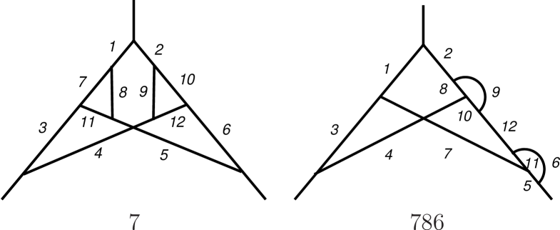
Figure 2: Graphs associated with the non-planar families 7 and 786 needed for the $n_{f}^{2}$ contribution to $F_{q}$ and $F_{b}$. The numbers $n$ next to the lines correspond to the indices of the propagators, i.e. to the $n^{\rm th}$ integer argument of the functions representing the integrals. In addition to the 12 propagators we have for each family six linear independent numerator factors. However, the corresponding indices are always zero for our master integrals.

The amplitudes, which contribute to the form factors, are prepared with the help of a well-tested setup. In a first step they are generated with qgraf [31]. For the fermionic form factors we have in total 1, 15 and 337 diagrams at one, two and three loops. At four-loop order we have 77 diagrams proportional to $n_{f}^{2}$ and one diagram proportional to $n_{f}^{3}$ (cf. Fig. 1 for sample diagrams). Next, we transform the output to FORM [32] notation using q2e and exp [33, 34]. The program exp furthermore maps each Feynman diagram to families for massless four-loop vertices with two different non-vanishing external momenta. Then we perform the Dirac algebra and obtain a set of input integrals for each family. It turns out that fourteen planar and two non-planar families are involved in the $n_{f}^{2}$ contribution of the fermionic form factors. The graphs associated with the non-planar families are shown in Fig. 2.

For the reduction to master integrals we use FIRE [35, 36, 37] which we apply in combination with LiteRed [38, 39]. Using FIRE we reveal 26 and 40 one-scale master integrals for the two non-planar families 7 and 786, respectively. For the analytical computation of these master integrals we follow the same strategy as in our previous work [19] which we briefly summarize for convenience:

1. We introduce a second mass scale by removing one of the quark momenta, $q_{2}$, from the light cone, i.e., we have $q_{2}^{2}\not=0$. Furthermore we define $q_{2}^{2}=xq^{2}$. With the help of FIRE we obtain 91 (101) two-scale master integrals for family 7 (786). The differential equations for these master integrals with respect to $x$ are obtained with the help of LiteRed [38, 39].

2. To solve our differential equations we turn from the primary basis to a canonical basis [40], where the corresponding master integrals satisfy a system of differential equations with the right-hand side proportional to $\epsilon$ and with only so-called Fuchsian singularities with respect to $x$. To construct our canonical basis we apply the private implementation of one of the authors (R.N.L.) of the algorithm discussed in Ref. [44].

3. Since our equations are in a canonical (or $\epsilon$) form, we write down a solution in a straightforward way order-by-order in $\epsilon$ in terms of harmonic polylogarithms (HPL) [47] with letters 0 and 1.

4. We determine the boundary conditions for the canonical master integrals, which are given as linear combinations of the primary master integrals, for $x=1$. The primary master integrals are regular at this point and become of propagator type. Thus they are expressed as linear combinations of 28 master integrals. Their analytic $\epsilon$-expansions are well-known [48, 49] up to weight 12. They have been cross-checked numerically in Ref. [50].

5. We solve our differential equations asymptotically near the point $x=0$ and fix these solutions by matching them to our solution at general $x$. Here we use the package HPL [51] to extract the leading order behaviour of the elements of the canonical basis in the limit $x\to 0$. The asymptotic solutions are linear combinations of powers $x^{k\epsilon}$ with $k=0,1,\ldots,8$. We pick up asymptotic terms with $k=0$ and obtain the so-called naive values of the canonical master integrals at $x=0$.

6. From the analytic results for the naive part we obtain analytical results for the sought-after one-scale master integrals after changing back to the primary basis.

To make the transition from the point $x=1$ to the point $x=0$ (cf. items 4. and 5. in the above list) we could apply the prescriptions explained in our previous paper [19]. However, we prefer to use the following slightly modified approach which we find more effective.

Let us assume that we have a differential equation in $\epsilon$-form

$$\partial_{x}\mathbf{J}(x)=\epsilon M(x)\mathbf{J}(x)\,,\quad M(x)=\sum_{a}\frac{M_{a}}{x-a}\,.$$ (7)

In our case, the sum over $a$ includes two terms, with $a=0$ and $a=1$. The formal solution of this equation is the path-ordered exponent

$$U(x,x_{0})=P\exp\left[\epsilon\int\limits_{x_{0}}^{x}{\rm d}\xi M(\xi)\right]\;.$$ (8)

This evolution operator can be readily expanded in $\epsilon$ with iterated integrals as coefficients. Since we want to put boundary conditions at $x=1$, we need to consider the limit $x_{0}\to 1$. Due to the presence of non-analytic terms of the form $(1-x_{0})^{\epsilon}$, this limit is not well defined when expanding in $\epsilon$. This can be fixed by factoring out the non-analytic piece

$$U(x,x_{0})=\widetilde{U}(x,x_{0})(1-x_{0})^{-\epsilon M_{1}}\;,$$ (9)

where $\widetilde{U}(x,x_{0})$ has a finite limit for $x_{0}\to 1$. Therefore, we can write down the general solution as

$$\mathbf{J}(x) = {\lim_{x_{0}\to 1}U(x,x_{0})\mathbf{C}_{x_{0}}}$$ (10)

$$= {\lim_{x_{0}\to 1}U(x,x_{0})(1-x_{0})^{-\epsilon M_{1}}(1-x_{0})^{\epsilon M_{1}}\mathbf{C}_{x_{0}}}$$

$$= \widetilde{U}(x,1)\mathbf{C}\,,$$

where $\mathbf{C}_{x_{0}}$ and $\mathbf{C}$ are column vectors of constants (depending on $\epsilon$). $\mathbf{C}_{x_{0}}$ depends in addition on $x_{0}$ whereas $\mathbf{C}$ does not. The “reduced” evolution operator $\widetilde{U}(x,1)$ can be easily expanded in $\epsilon$ with the coefficients being harmonic polylogarithms of $x$. The column of constants can be fixed by considering the asymptotics of the canonical master integrals for $x\to 1$. In this limit we have

$$\mathbf{J}(x)\sim(1-x)^{\epsilon M_{1}}\mathbf{C}\,.$$ (11)

Note, that we want to relate $\mathbf{C}$ to the coefficients of the asymptotic expansion of the primary master integrals, $\mathbf{j}(x)$, which are obtained from the canonical ones via $\mathbf{j}(x)=T(\epsilon,x)\mathbf{J}(x)$. This might seem nontrivial since $T(\epsilon,x)$ (and $T^{-1}(\epsilon,x)$) have multiple poles for $x\to 1$. Therefore, we need to know several terms of the asymptotic expansion of $\mathbf{J}(x)$. We identically rewrite Eq. (10) as

$$\mathbf{J}(x)=(1-x)^{\epsilon M_{1}}{\overline{U}}(x,1)\mathbf{C}\,.$$ (12)

The operator $\overline{U}(x,1)=(1-x)^{-\epsilon M_{1}}\widetilde{U}(x,1)$ can be expanded in $1-x$ up to sufficiently high power which makes it possible to connect the column of constants in $\mathbf{C}$ with the specific coefficients of the asymptotic expansion of the primary master integrals at $x=1$.

We stress that the described method is extremely economic in the sense that the overall number of asymptotic coefficients of the primary master integrals (each being a function of $\epsilon$) to be fixed can be minimized and is equal to the number of constants in $\mathbf{C}$. In addition, since the integrals are all analytic in the point $x=1$, we set to zero all coefficients in front of non-integer powers of $1-x$ in the generic solution. This reduces even further the number of coefficients which we need to calculate. We finally find that the boundary conditions are entirely fixed by those entries of $\mathbf{j}(1)$ which are present among the 28 integrals from Refs. [48, 49]. Note that within our present approach it is not necessary to calculate several expansion terms of the primary masters near $x=1$, in contrast to Ref. [19]. The analysis at $x=0$ is simplified in a similar way.

Repeating similar considerations for the point $x=0$, we finally connect the coefficients of the asymptotic expansion of the primary master integrals for $x\to 0$ with those for $x\to 1$. In particular, we extract the naive values of the primary master integrals at $x=0$.

Following the procedure outlined in this Section we could compute all master integrals contained in the families 7 and 786 up to weight 8. Analytic expressions for the 24 non-planar master integrals are given in the Appendix.

3 $n_{f}^{2}$ results for form factors

In this Section we discuss the results which we have obtained for the various form factors using the techniques outlined in the previous Section and the analytic results for the master integrals given in the Appendix. We have used a general QCD gauge parameter $\xi$ in the gluon propagator and have expanded each Feynman amplitude up to the linear term. We have checked that the coefficient of $\xi$ vanishes for the bare form factors once all master integrals are mapped to a minimal set.

3.1 Photon quark form factor

For the $n_{f}^{2}$ term of the photon quark form factor only the following three non-planar master integrals are needed:

$$G_{110110100111}^{\text{(7)}},G_{110110100112}^{\text{(7)}},G_{111101101110}^{\text{(786)}}$$ (13)

Analytic results are given in the Appendix. We insert these results together with the ones for the planar master integrals, expand in $\epsilon$ and renormalize $\alpha_{s}$. After taking the logarithm we can compare to Eq. (4) and extract the cusp and collinear anomalous dimension. We obtain

$$\gamma_{\rm cusp}^{0} = 4\,,$$

$$\gamma_{\rm cusp}^{1} = \left(\frac{268}{9}-\frac{4\pi^{2}}{3}\right)C_{A}-\frac{40n_{f}}{9}\,,$$

$$\gamma_{\rm cusp}^{2} = C_{A}^{2}\left(\frac{88\zeta_{3}}{3}+\frac{44\pi^{4}}{45}-\frac{536\pi^{2}}{27}+\frac{490}{3}\right)$$

$$\mbox{}+n_{f}\left[C_{A}\left(-\frac{112\zeta_{3}}{3}+\frac{80\pi^{2}}{27}-\frac{836}{27}\right)+C_{F}\left(32\zeta_{3}-\frac{110}{3}\right)\right]-\frac{16n_{f}^{2}}{27}\,,$$

$$\gamma_{\rm cusp}^{3} = \gamma_{\text{cusp}}^{3,n_{f}^{0}}+\gamma_{\text{cusp}}^{3,n_{f}^{1}}n_{f}$$ (14)

$$\mbox{}+n_{f}^{2}\Bigg{[}C_{A}\left(\frac{2240\zeta_{3}}{27}-\frac{56\pi^{4}}{135}-\frac{304\pi^{2}}{243}+\frac{923}{81}\right)+C_{F}\left(-\frac{640\zeta_{3}}{9}+\frac{16\pi^{4}}{45}+\frac{2392}{81}\right)\Bigg{]}$$

$$\mbox{}+\left(\frac{64\zeta_{3}}{27}-\frac{32}{81}\right)n_{f}^{3}\,,$$

and

$$\gamma_{q}^{0} = -3C_{F}\,,$$

$$\gamma_{q}^{1} = \left(26\zeta_{3}-\frac{11\pi^{2}}{6}-\frac{961}{54}\right)C_{A}C_{F}+\left(\frac{65}{27}+\frac{\pi^{2}}{3}\right)C_{F}n_{f}+\left(-24\zeta_{3}+2\pi^{2}-\frac{3}{2}\right)C_{F}^{2}\,,$$

$$\gamma_{q}^{2} = n_{f}\Bigg{[}\left(-\frac{964\zeta_{3}}{27}+\frac{11\pi^{4}}{45}+\frac{1297\pi^{2}}{243}-\frac{8659}{729}\right)C_{A}C_{F}+\left(\frac{256\zeta_{3}}{9}-\frac{14\pi^{4}}{27}-\frac{13\pi^{2}}{9}\right.$$

$$\left.\mbox{}+\frac{2953}{54}\right)C_{F}^{2}\Bigg{]}+\left(-\frac{8}{3}\pi^{2}\zeta_{3}-\frac{844\zeta_{3}}{3}-120\zeta_{5}+\frac{247\pi^{4}}{135}+\frac{205\pi^{2}}{9}-\frac{151}{4}\right)C_{A}C_{F}^{2}$$

$$\mbox{}+\left(-\frac{44}{9}\pi^{2}\zeta_{3}+\frac{3526\zeta_{3}}{9}-136\zeta_{5}-\frac{83\pi^{4}}{90}-\frac{7163\pi^{2}}{486}-\frac{139345}{2916}\right)C_{A}^{2}C_{F}$$

$$\mbox{}+\left(-\frac{8\zeta_{3}}{27}-\frac{10\pi^{2}}{27}+\frac{2417}{729}\right)C_{F}n_{f}^{2}+\left(\frac{16\pi^{2}\zeta_{3}}{3}-68\zeta_{3}+240\zeta_{5}-\frac{8\pi^{4}}{5}-3\pi^{2}\right.$$

$$\left.\mbox{}-\frac{29}{2}\right)C_{F}^{3}\,,$$

$$\gamma_{q}^{3} = n_{f}^{2}\Bigg{[}\left(-\frac{64}{27}\pi^{2}\zeta_{3}-\frac{7436\zeta_{3}}{243}+\frac{592\zeta_{5}}{9}-\frac{19\pi^{4}}{135}-\frac{41579\pi^{2}}{8748}+\frac{97189}{34992}\right)C_{A}C_{F}$$ (15)

$$\mbox{}+\left(\frac{56\pi^{2}\zeta_{3}}{27}+\frac{2116\zeta_{3}}{81}-\frac{520\zeta_{5}}{9}+\frac{1004\pi^{4}}{1215}-\frac{493\pi^{2}}{81}-\frac{9965}{972}\right)C_{F}^{2}\Bigg{]}$$

$$\mbox{}+\left(-\frac{712\zeta_{3}}{243}-\frac{16\pi^{4}}{1215}-\frac{4\pi^{2}}{81}+\frac{18691}{6561}\right)C_{F}n_{f}^{3}+n_{f}\gamma_{q}^{3,n_{f}^{1}}+\gamma_{q}^{3,n_{f}^{0}}\,,$$

where $\zeta_{n}$ is Riemann’s zeta function evaluated at $n$. The coefficients $\gamma_{\text{cusp}}^{3,n_{f}^{0}}$, $\gamma_{\text{cusp}}^{3,n_{f}^{1}}$, $\gamma_{q}^{3,n_{f}^{0}}$ and $\gamma_{q}^{3,n_{f}^{1}}$ are only known in the large-$N_{c}$ limit [18, 19]. The one- to three-loop results for $\gamma_{\text{cusp}}$ and $\gamma_{q}$ can be found in Refs. [52, 53, 54, 55, 12, 29, 13] and the $n_{f}^{3}$ terms of $\gamma_{\text{cusp}}^{3}$ has been obtained in Refs. [56, 57]. The $n_{f}^{2}$ term of $\gamma_{\text{cusp}}^{3}$ agrees with [58]. The terms in $\gamma_{q}^{3}$ which are beyond the large-$N_{c}$ limit are new.

For completeness we also present results for the finite part of $F_{q}$ which is conveniently done for the bare form factors since at each loop order the $\mu$ dependence factorizes. In analogy to Eq. (3) we write

$$\log(F_{q}) = \sum_{n\geq 1}\left(\frac{\alpha_{s}^{0}}{4\pi}\right)^{n}\left(\frac{\mu^{2}}{-q^{2}-i0}\right)^{n\epsilon}\log(F_{q})|^{(n)}\,.$$ (16)

The $n_{f}^{3}$ and $n_{f}^{2}$ terms of $\log(F_{q})|^{(4)}$ are given by

$$\log(F_{q})|^{(4)}_{n_{f}^{2},n_{f}^{3}}=$$ (17)

$$\mbox{}\frac{1}{\epsilon^{5}}\Bigg{[}\frac{1}{27}C_{F}n_{f}^{3}-\frac{11}{18}C_{A}C_{F}n_{f}^{2}\Bigg{]}+\frac{1}{\epsilon^{4}}\Bigg{[}n_{f}^{2}\left(\left(\frac{\pi^{2}}{18}-\frac{395}{54}\right)C_{A}C_{F}-\frac{2C_{F}^{2}}{9}\right)+\frac{11}{27}C_{F}n_{f}^{3}\Bigg{]}$$

$$\mbox{}+\frac{1}{\epsilon^{3}}\Bigg{[}n_{f}^{2}\left(\left(\frac{19\zeta_{3}}{3}-\frac{5\pi^{2}}{6}-\frac{75619}{1296}\right)C_{A}C_{F}+\left(-6\zeta_{3}+\frac{2\pi^{2}}{3}-\frac{481}{108}\right)C_{F}^{2}\right)$$

$$\mbox{}+\left(\frac{254}{81}+\frac{5\pi^{2}}{81}\right)C_{F}n_{f}^{3}\Bigg{]}+\frac{1}{\epsilon^{2}}\Bigg{[}n_{f}^{2}\left(\left(\frac{2170\zeta_{3}}{27}+\frac{13\pi^{4}}{60}-\frac{1022\pi^{2}}{81}-\frac{2953141}{7776}\right)C_{A}C_{F}\right.$$

$$\left.\mbox{}+\left(-52\zeta_{3}-\frac{7\pi^{4}}{90}+\frac{197\pi^{2}}{27}-\frac{14309}{324}\right)C_{F}^{2}\right)+\left(-\frac{82\zeta_{3}}{81}+\frac{55\pi^{2}}{81}+\frac{29023}{1458}\right)C_{F}n_{f}^{3}\Bigg{]}$$

$$\mbox{}+\frac{1}{\epsilon}\Bigg{[}n_{f}^{2}\left(\left(-\frac{206}{27}\pi^{2}\zeta_{3}+\frac{61459\zeta_{3}}{81}+\frac{784\zeta_{5}}{9}+\frac{503\pi^{4}}{810}-\frac{424399\pi^{2}}{3888}-\frac{102630137}{46656}\right)C_{A}C_{F}\right.$$

$$\left.\mbox{}+\left(\frac{74\pi^{2}\zeta_{3}}{9}-\frac{15121\zeta_{3}}{27}+62\zeta_{5}+\frac{31\pi^{4}}{135}+\frac{16993\pi^{2}}{324}-\frac{1308889}{3888}\right)C_{F}^{2}\right)$$

$$\mbox{}+\left(-\frac{902\zeta_{3}}{81}+\frac{151\pi^{4}}{2430}+\frac{1270\pi^{2}}{243}+\frac{331889}{2916}\right)C_{F}n_{f}^{3}\Bigg{]}+n_{f}^{2}\left(\left(-\frac{1714\zeta_{3}^{2}}{3}-\frac{218\pi^{2}\zeta_{3}}{9}\right.\right.$$

$$\left.\left.\mbox{}+\frac{2897315\zeta_{3}}{486}+\frac{150886\zeta_{5}}{135}-\frac{709\pi^{6}}{17010}-\frac{1861\pi^{4}}{2430}-\frac{5825827\pi^{2}}{7776}-\frac{3325501813}{279936}\right)C_{A}C_{F}\right.$$

$$\left.\mbox{}+\left(\frac{2702\zeta_{3}^{2}}{3}+\frac{1820\pi^{2}\zeta_{3}}{27}-\frac{859249\zeta_{3}}{162}+\frac{1580\zeta_{5}}{3}+\frac{17609\pi^{6}}{17010}+\frac{1141\pi^{4}}{1620}+\frac{76673\pi^{2}}{243}\right.\right.$$

$$\left.\left.\mbox{}-\frac{25891301}{11664}\right)C_{F}^{2}\right)+\left(-\frac{410}{243}\pi^{2}\zeta_{3}-\frac{20828\zeta_{3}}{243}-\frac{2194\zeta_{5}}{135}+\frac{1661\pi^{4}}{2430}+\frac{145115\pi^{2}}{4374}\right.$$

$$\left.\mbox{}+\frac{10739263}{17496}\right)C_{F}n_{f}^{3}\,.$$

The four-loop term in the large-$N_{c}$ limit can be extracted from Ref. [19]; all other terms are new.

3.2 Higgs quark form factor

The calculation of $F_{b}$ proceeds in close analogy to $F_{q}$. It is interesting to note that about 20% fewer integrals are needed in the case of $F_{b}$. However, the complexity of the most complicated integrals is the same and thus the CPU time needed for the reduction to master integrals is comparable for the two calculations.

After renormalizing $\alpha_{s}$ and $y$ and taking the logarithm we again compare to Eq. (4) and extract the cusp and collinear anomalous dimension. We obtain the same results as in Eqs. (14) and (15) which constitutes a strong check for our calculation.

If we define $\log(F_{b})$ expressed in terms of bare $\alpha_{s}$ and $y$ in analogy to Eq. (16) we get for the $n_{f}^{3}$ and $n_{f}^{2}$ terms of $\log(F_{b})|^{(4)}$

$$\log(F_{b})|^{(4)}_{n_{f}^{2},n_{f}^{3}}=$$

$$\mbox{}\frac{1}{\epsilon^{5}}\Bigg{[}\frac{1}{27}C_{F}n_{f}^{3}-\frac{11}{18}C_{A}C_{F}n_{f}^{2}\Bigg{]}+\frac{1}{\epsilon^{4}}\Bigg{[}n_{f}^{2}\left(\left(\frac{\pi^{2}}{18}-\frac{197}{54}\right)C_{A}C_{F}-\frac{2C_{F}^{2}}{9}\right)+\frac{5}{27}C_{F}n_{f}^{3}\Bigg{]}$$

$$\mbox{}+\frac{1}{\epsilon^{3}}\Bigg{[}n_{f}^{2}\left(\left(\frac{19\zeta_{3}}{3}-\frac{5\pi^{2}}{6}-\frac{19819}{1296}\right)C_{A}C_{F}+\left(-6\zeta_{3}+\frac{2\pi^{2}}{3}-\frac{283}{108}\right)C_{F}^{2}\right)$$

$$\mbox{}+\left(\frac{65}{81}+\frac{5\pi^{2}}{81}\right)C_{F}n_{f}^{3}\Bigg{]}+\frac{1}{\epsilon^{2}}\Bigg{[}n_{f}^{2}\left(\left(\frac{1846\zeta_{3}}{27}+\frac{13\pi^{4}}{60}-\frac{491\pi^{2}}{81}-\frac{417697}{7776}\right)C_{A}C_{F}\right.$$

$$\left.\mbox{}+\left(-64\zeta_{3}-\frac{7\pi^{4}}{90}+\frac{119\pi^{2}}{27}-\frac{1244}{81}\right)C_{F}^{2}\right)+\left(-\frac{82\zeta_{3}}{81}+\frac{25\pi^{2}}{81}+\frac{2537}{729}\right)C_{F}n_{f}^{3}\Bigg{]}$$

$$\mbox{}+\frac{1}{\epsilon}\Bigg{[}n_{f}^{2}\left(\left(-\frac{206}{27}\pi^{2}\zeta_{3}+\frac{35089\zeta_{3}}{81}+\frac{784\zeta_{5}}{9}+\frac{251\pi^{4}}{810}-\frac{121495\pi^{2}}{3888}-\frac{7185425}{46656}\right)C_{A}C_{F}\right.$$

$$\left.\mbox{}+\left(\frac{74\pi^{2}\zeta_{3}}{9}-\frac{12079\zeta_{3}}{27}+62\zeta_{5}-\frac{38\pi^{4}}{135}+\frac{6871\pi^{2}}{324}-\frac{258229}{3888}\right)C_{F}^{2}\right)+\left(-\frac{410\zeta_{3}}{81}\right.$$

$$\left.\mbox{}+\frac{151\pi^{4}}{2430}+\frac{325\pi^{2}}{243}+\frac{11408}{729}\right)C_{F}n_{f}^{3}\Bigg{]}+\Bigg{[}n_{f}^{2}\left(\left(-\frac{1714\zeta_{3}^{2}}{3}+\frac{14\pi^{2}\zeta_{3}}{9}+\frac{1209401\zeta_{3}}{486}\right.\right.$$

$$\left.\left.\mbox{}+\frac{144946\zeta_{5}}{135}-\frac{709\pi^{6}}{17010}+\frac{2129\pi^{4}}{2430}-\frac{1168375\pi^{2}}{7776}-\frac{73152481}{279936}\right)C_{A}C_{F}+\left(\frac{2702\zeta_{3}^{2}}{3}\right.\right.$$

$$\left.\left.\mbox{}+\frac{632\pi^{2}\zeta_{3}}{27}-\frac{489655\zeta_{3}}{162}-760\zeta_{5}+\frac{17609\pi^{6}}{17010}-\frac{4693\pi^{4}}{1620}+\frac{94031\pi^{2}}{972}-\frac{2614421}{11664}\right)C_{F}^{2}\right)$$

$$\mbox{}+\left(-\frac{410}{243}\pi^{2}\zeta_{3}-\frac{5330\zeta_{3}}{243}-\frac{2194\zeta_{5}}{135}+\frac{151\pi^{4}}{486}+\frac{12685\pi^{2}}{2187}+\frac{159908}{2187}\right)C_{F}n_{f}^{3}\Bigg{]}\,.$$

To obtain this result the $\epsilon^{2}$ terms of the three-loop form factor are needed. We refrain from listing them explicitly but present the expressions, which are not yet available in the literature, in the ancillary file [30].

4 Conclusions

We have computed the complete $n_{f}^{2}$ contributions for the massless four-loop fermionic form factors $F_{q}$ and $F_{b}$ and provide the corresponding cusp and collinear anomalous dimensions. This requires to consider two non-planar integral families. We systematically construct the solution applying algorithmic procedures and obtain analytic results for all master integrals contained in these families. Although only three non-planar master integrals are needed for the form factors we present analytic results for all 24 non-planar integrals, one of the main results of this paper. They constitute important ingredients for future calculations, e.g., the $n_{f}^{1}$ and the $n_{f}$-independent parts. Furthermore, we extend the three-loop result for the Higgs fermion form factor to order $\epsilon^{2}$. All analytic results can be downloaded from [30].

Appendix: Explicit results for non-planar master integrals

The 26 master integrals in family 7 (cf. Fig. 2) are

$$G_{000001111001}^{\text{(7)}},G_{000000111111}^{\text{(7)}},G_{000001111110}^{\text{(7)}},G_{000101111100}^{\text{(7)}},G_{010000110111}^{\text{(7)}},G_{110000011011}^{\text{(7)}},$$

$$G_{000001111111}^{\text{(7)}},G_{000101111110}^{\text{(7)}},G_{010000111111}^{\text{(7)}},G_{010001111011}^{\text{(7)}},G_{010001111012}^{\text{(7)}},G_{010110110101}^{\text{(7)}},$$

$$G_{011010110101}^{\text{(7)}},G_{110001101011}^{\text{(7)}},G_{000110111111}^{\text{(7)}},G_{001111111100}^{\text{(7)}},G_{010010111111}^{\text{(7)}},G_{010110110111}^{\text{(7)}},$$

$$G_{011010111101}^{\text{(7)}},G_{011010111102}^{\text{(7)}},G_{011011111001}^{\text{(7)}},G_{110000111111}^{\text{(7)}},G_{110001111011}^{\text{(7)}},G_{110011101011}^{\text{(7)}},$$

$$G_{110110100111}^{\text{(7)}},G_{110110100112}^{\text{(7)}},$$ (19)

and the 40 master integrals in family 786 are chosen as

$$G_{001010011010}^{\text{(786)}},G_{001001111010}^{\text{(786)}},G_{011010001110}^{\text{(786)}},G_{100010011110}^{\text{(786)}},G_{100101001110}^{\text{(786)}},G_{100101011010}^{\text{(786)}},$$

$$G_{110010010110}^{\text{(786)}},G_{011001101110}^{\text{(786)}},G_{011001110110}^{\text{(786)}},G_{011010011110}^{\text{(786)}},G_{100001111110}^{\text{(786)}},G_{100101111010}^{\text{(786)}},$$

$$G_{100110011011}^{\text{(786)}},G_{100110011110}^{\text{(786)}},G_{101001011110}^{\text{(786)}},G_{101001011120}^{\text{(786)}},G_{110001110110}^{\text{(786)}},G_{110110001110}^{\text{(786)}},$$

$$G_{111001001110}^{\text{(786)}},G_{011001111110}^{\text{(786)}},G_{100101111110}^{\text{(786)}},G_{100111011110}^{\text{(786)}},G_{101001111110}^{\text{(786)}},G_{101011011110}^{\text{(786)}},$$

$$G_{101101111010}^{\text{(786)}},G_{101110011011}^{\text{(786)}},G_{101111011010}^{\text{(786)}},G_{110101101110}^{\text{(786)}},G_{111001110110}^{\text{(786)}},G_{111010010111}^{\text{(786)}},$$

$$G_{111010010112}^{\text{(786)}},G_{111010011110}^{\text{(786)}},G_{111011010110}^{\text{(786)}},G_{111110001110}^{\text{(786)}},G_{101111011110}^{\text{(786)}},G_{111001111110}^{\text{(786)}},$$

$$G_{111011011110}^{\text{(786)}},G_{111011011120}^{\text{(786)}},G_{111101101110}^{\text{(786)}},G_{111111001110}^{\text{(786)}}.$$ (20)

The planar integrals have already been used in Ref. [19] to obtain $F_{q}$ in the large-$N_{c}$ limit. Their analytic results will be provided in Ref. [21]. Here, we concentrate on the non-planar integrals.

Family 7 has twelve non-planar master integrals. Five of them can be mapped to family 786 using

$$G_{010110110111}^{\text{(7)}} \to G_{101001111110}^{\text{(786)}}\,,$$

$$G_{011011111001}^{\text{(7)}} \to G_{101110011011}^{\text{(786)}}\,,$$

$$G_{110001111011}^{\text{(7)}} \to G_{111010011110}^{\text{(786)}}\,,$$

$$G_{110011101011}^{\text{(7)}} \to G_{111110001110}^{\text{(786)}}\,,$$

$$G_{110110100111}^{\text{(7)}} \to G_{111010010111}^{\text{(786)}}\,.$$ (21)

The analytic results of the remaining seven integrals expanded up to weight eight are given by

$$G_{000110111111}^{\text{(7)}}=$$

$$\frac{5\zeta_{5}}{\epsilon}+9\zeta_{3}^{2}+55\zeta_{5}+\frac{\pi^{6}}{30}+\epsilon\Bigg{[}99\zeta_{3}^{2}+\frac{67\pi^{4}\zeta_{3}}{90}-\frac{47\pi^{2}\zeta_{5}}{3}+455\zeta_{5}+\frac{591\zeta_{7}}{2}+\frac{11\pi^{6}}{30}\Bigg{]}$$

$$\mbox{}+\epsilon^{2}\Bigg{[}-\frac{76s_{8a}}{5}-5\pi^{2}\zeta_{3}^{2}+819\zeta_{3}^{2}-\frac{302\zeta_{5}\zeta_{3}}{3}+\frac{737\pi^{4}\zeta_{3}}{90}-\frac{517\pi^{2}\zeta_{5}}{3}+3355\zeta_{5}+\frac{6501\zeta_{7}}{2}$$

$$\mbox{}+\frac{23689\pi^{8}}{378000}+\frac{91\pi^{6}}{30}\Bigg{]}\,,$$

$$G_{001111111100}^{\text{(7)}}=$$

$$\frac{1}{2\epsilon^{4}}+\frac{7}{\epsilon^{3}}+\frac{1}{\epsilon^{2}}\Bigg{[}63-\frac{\pi^{2}}{2}\Bigg{]}+\frac{1}{\epsilon}\Bigg{[}-\frac{107\zeta_{3}}{3}-7\pi^{2}+465\Bigg{]}+-\frac{1498\zeta_{3}}{3}-\frac{119\pi^{4}}{180}-63\pi^{2}$$

$$\mbox{}+3069+\epsilon\Bigg{[}33\pi^{2}\zeta_{3}-4506\zeta_{3}-\frac{2437\zeta_{5}}{5}-\frac{833\pi^{4}}{90}-465\pi^{2}+18873\Bigg{]}$$

$$\mbox{}+\epsilon^{2}\Bigg{[}\frac{11593\zeta_{3}^{2}}{9}+462\pi^{2}\zeta_{3}-33446\zeta_{3}-\frac{34118\zeta_{5}}{5}-\frac{6721\pi^{6}}{11340}-\frac{7519\pi^{4}}{90}-3069\pi^{2}$$

$$\mbox{}+110621\Bigg{]}+\epsilon^{3}\Bigg{[}\frac{162302\zeta_{3}^{2}}{9}+\frac{12757\pi^{4}\zeta_{3}}{270}+4170\pi^{2}\zeta_{3}-222702\zeta_{3}+\frac{6871\pi^{2}\zeta_{5}}{15}$$

$$\mbox{}-\frac{307822\zeta_{5}}{5}-\frac{46762\zeta_{7}}{7}-\frac{6721\pi^{6}}{810}-\frac{55841\pi^{4}}{90}-18873\pi^{2}+626545\Bigg{]}$$

$$\mbox{}+\epsilon^{4}\Bigg{[}-712s_{8a}-\frac{10169}{9}\pi^{2}\zeta_{3}^{2}+163134\zeta_{3}^{2}+\frac{528478\zeta_{5}\zeta_{3}}{15}+\frac{89299\pi^{4}\zeta_{3}}{135}+30966\pi^{2}\zeta_{3}$$

$$\mbox{}-1386486\zeta_{3}+\frac{96194\pi^{2}\zeta_{5}}{15}-456778\zeta_{5}-93524\zeta_{7}-\frac{43481\pi^{8}}{680400}-\frac{60439\pi^{6}}{810}-\frac{41349\pi^{4}}{10}$$

$$\mbox{}-110621\pi^{2}+3459765\Bigg{]}\,,$$

$$G_{010010111111}^{\text{(7)}}=$$

$$\frac{5\zeta_{5}}{\epsilon}+7\zeta_{3}^{2}-2\pi^{2}\zeta_{3}+45\zeta_{5}+\frac{71\pi^{6}}{2268}$$

$$\mbox{}+\epsilon\Bigg{[}47\zeta_{3}^{2}-\frac{7\pi^{4}\zeta_{3}}{18}-34\pi^{2}\zeta_{3}+\frac{40\pi^{2}\zeta_{5}}{3}+285\zeta_{5}+\frac{907\zeta_{7}}{4}+\frac{3023\pi^{6}}{11340}\Bigg{]}$$

$$\mbox{}+\epsilon^{2}\Bigg{[}-\frac{582s_{8a}}{5}+\frac{53}{3}\pi^{2}\zeta_{3}^{2}+127\zeta_{3}^{2}-\frac{722\zeta_{5}\zeta_{3}}{3}-\frac{367\pi^{4}\zeta_{3}}{90}-386\pi^{2}\zeta_{3}+128\pi^{2}\zeta_{5}$$

$$\mbox{}+1425\zeta_{5}+\frac{9097\zeta_{7}}{4}+\frac{341261\pi^{8}}{1701000}+\frac{2473\pi^{6}}{1620}\Bigg{]}\,,$$

$$G_{011010111101}^{\text{(7)}}=$$

$$\frac{3\zeta_{3}}{2\epsilon^{2}}+\frac{1}{\epsilon}\Bigg{[}\frac{39\zeta_{3}}{2}+\frac{11\pi^{4}}{360}\Bigg{]}+-\frac{5}{2}\pi^{2}\zeta_{3}+\frac{351\zeta_{3}}{2}+\frac{3\zeta_{5}}{2}+\frac{143\pi^{4}}{360}$$

$$\mbox{}+\epsilon\Bigg{[}-\frac{263\zeta_{3}^{2}}{2}-\frac{57\pi^{2}\zeta_{3}}{2}+\frac{2715\zeta_{3}}{2}+\frac{79\zeta_{5}}{2}-\frac{2519\pi^{6}}{22680}+\frac{143\pi^{4}}{40}\Bigg{]}$$

$$\mbox{}+\epsilon^{2}\Bigg{[}-\frac{3299\zeta_{3}^{2}}{2}-\frac{2491\pi^{4}\zeta_{3}}{540}-\frac{433\pi^{2}\zeta_{3}}{2}+\frac{19383\zeta_{3}}{2}-\frac{269\pi^{2}\zeta_{5}}{6}+\frac{1111\zeta_{5}}{2}$$

$$\mbox{}-\frac{2213\zeta_{7}}{4}-\frac{29219\pi^{6}}{22680}+\frac{1991\pi^{4}}{72}\Bigg{]}+\epsilon^{3}\Bigg{[}316s_{8a}+\frac{755}{6}\pi^{2}\zeta_{3}^{2}-\frac{28491\zeta_{3}^{2}}{2}-\frac{13531\zeta_{5}\zeta_{3}}{5}$$

$$\mbox{}-\frac{6329\pi^{4}\zeta_{3}}{108}-\frac{2677\pi^{2}\zeta_{3}}{2}+\frac{131859\zeta_{3}}{2}-\frac{3263\pi^{2}\zeta_{5}}{6}+\frac{11955\zeta_{5}}{2}-\frac{13445\zeta_{7}}{2}-\frac{13939\pi^{8}}{24300}$$

$$\mbox{}-\frac{2811\pi^{6}}{280}+\frac{71071\pi^{4}}{360}\Bigg{]}\,,$$

$$G_{011010111102}^{\text{(7)}}=$$

$$\frac{1}{\epsilon^{6}}\Bigg{[}-\frac{1}{36}\Bigg{]}+\frac{1}{\epsilon^{5}}\Bigg{[}-\frac{1}{18}\Bigg{]}+\frac{1}{\epsilon^{4}}\Bigg{[}-\frac{1}{9}\Bigg{]}+\frac{1}{\epsilon^{3}}\Bigg{[}\frac{89\zeta_{3}}{54}-\frac{2}{9}\Bigg{]}+\frac{1}{\epsilon^{2}}\Bigg{[}\frac{89\zeta_{3}}{27}+\frac{7\pi^{4}}{120}-\frac{4}{9}\Bigg{]}$$

$$\mbox{}+\frac{1}{\epsilon}\Bigg{[}\frac{7\pi^{2}\zeta_{3}}{9}+\frac{178\zeta_{3}}{27}+\frac{2117\zeta_{5}}{90}+\frac{7\pi^{4}}{60}-\frac{8}{9}\Bigg{]}$$

$$\mbox{}-\frac{9271\zeta_{3}^{2}}{162}+\frac{14\pi^{2}\zeta_{3}}{9}+\frac{356\zeta_{3}}{27}+\frac{2117\zeta_{5}}{45}+\frac{2573\pi^{6}}{34020}+\frac{7\pi^{4}}{30}-\frac{16}{9}+\epsilon\Bigg{[}-\frac{9271\zeta_{3}^{2}}{81}$$

$$\mbox{}-\frac{667\pi^{4}\zeta_{3}}{180}+\frac{28\pi^{2}\zeta_{3}}{9}+\frac{712\zeta_{3}}{27}+9\pi^{2}\zeta_{5}+\frac{4234\zeta_{5}}{45}+\frac{21151\zeta_{7}}{252}+\frac{2573\pi^{6}}{17010}+\frac{7\pi^{4}}{15}-\frac{32}{9}\Bigg{]}$$

$$\mbox{}+\epsilon^{2}\Bigg{[}\frac{848s_{8a}}{5}-\frac{1528}{27}\pi^{2}\zeta_{3}^{2}-\frac{18542\zeta_{3}^{2}}{81}-\frac{230803\zeta_{5}\zeta_{3}}{135}-\frac{667\pi^{4}\zeta_{3}}{90}+\frac{344\pi^{2}\zeta_{3}}{9}+\frac{1424\zeta_{3}}{27}$$

$$\mbox{}+18\pi^{2}\zeta_{5}+\frac{15668\zeta_{5}}{45}+\frac{21151\zeta_{7}}{126}-\frac{500903\pi^{8}}{3402000}+\frac{2573\pi^{6}}{8505}+\frac{14\pi^{4}}{15}-\frac{64}{9}\Bigg{]}\,,$$

$$G_{110000111111}^{\text{(7)}}=$$

$$+\frac{1}{\epsilon^{4}}\Bigg{[}\frac{1}{12}\Bigg{]}+\frac{1}{\epsilon^{3}}+\frac{1}{\epsilon^{2}}\Bigg{[}\frac{91}{12}-\frac{\pi^{2}}{36}\Bigg{]}+\frac{1}{\epsilon}\Bigg{[}-\frac{37\zeta_{3}}{9}-\frac{\pi^{2}}{3}+\frac{93}{2}\Bigg{]}+\frac{\pi^{2}\zeta_{3}}{3}-48\zeta_{3}+\frac{5\zeta_{5}}{3}$$

$$\mbox{}-\frac{37\pi^{4}}{540}-\frac{95\pi^{2}}{36}+\frac{3025}{12}+\epsilon\Bigg{[}\frac{5\zeta_{3}^{2}}{3}+\frac{115\pi^{2}\zeta_{3}}{27}-\frac{3131\zeta_{3}}{9}-\frac{2038\zeta_{5}}{45}+\frac{88\pi^{6}}{8505}-\frac{193\pi^{4}}{270}$$

$$\mbox{}-\frac{955\pi^{2}}{54}+1262\Bigg{]}+\epsilon^{2}\Bigg{[}\frac{2543\zeta_{3}^{2}}{27}+\frac{71\pi^{4}\zeta_{3}}{270}+\frac{1039\pi^{2}\zeta_{3}}{27}-\frac{53390\zeta_{3}}{27}-\frac{\pi^{2}\zeta_{5}}{9}-\frac{79163\zeta_{5}}{135}$$

$$\mbox{}+\frac{407\zeta_{7}}{12}-\frac{799\pi^{6}}{14580}-\frac{7261\pi^{4}}{1620}-\frac{35449\pi^{2}}{324}+\frac{71767}{12}\Bigg{]}+\epsilon^{3}\Bigg{[}-\frac{346s_{8a}}{15}-\frac{94}{3}\pi^{2}\zeta_{3}^{2}$$

$$\mbox{}+\frac{25763\zeta_{3}^{2}}{27}-\frac{1694\zeta_{5}\zeta_{3}}{9}+\frac{1073\pi^{4}\zeta_{3}}{270}+\frac{26051\pi^{2}\zeta_{3}}{81}-\frac{761281\zeta_{3}}{81}+\frac{383\pi^{2}\zeta_{5}}{135}-\frac{1657792\zeta_{5}}{405}$$

$$\mbox{}-\frac{278843\zeta_{7}}{252}-\frac{461\pi^{8}}{70875}-\frac{14227\pi^{6}}{15309}-\frac{24929\pi^{4}}{1215}-\frac{157496\pi^{2}}{243}+\frac{54491}{2}\Bigg{]}\,,$$

$$G_{110110100112}^{\text{(7)}}=$$ (22)

$$+\frac{1}{\epsilon^{4}}\Bigg{[}-\frac{\pi^{2}}{36}\Bigg{]}+\frac{1}{\epsilon^{3}}\Bigg{[}-\frac{\zeta_{3}}{3}-\frac{\pi^{2}}{18}\Bigg{]}+\frac{1}{\epsilon^{2}}\Bigg{[}-\frac{2\zeta_{3}}{3}-\frac{\pi^{4}}{30}-\frac{\pi^{2}}{9}\Bigg{]}$$

$$\mbox{}+\frac{1}{\epsilon}\Bigg{[}\frac{37\pi^{2}\zeta_{3}}{27}-\frac{4\zeta_{3}}{3}+6\zeta_{5}-\frac{\pi^{4}}{15}-\frac{2\pi^{2}}{9}\Bigg{]}+\frac{361\zeta_{3}^{2}}{9}+\frac{74\pi^{2}\zeta_{3}}{27}-\frac{8\zeta_{3}}{3}+12\zeta_{5}+\frac{71\pi^{6}}{1890}$$

$$\mbox{}-\frac{2\pi^{4}}{15}-\frac{4\pi^{2}}{9}+\epsilon\Bigg{[}\frac{722\zeta_{3}^{2}}{9}+\frac{44\pi^{4}\zeta_{3}}{15}+\frac{148\pi^{2}\zeta_{3}}{27}-\frac{16\zeta_{3}}{3}+\frac{886\pi^{2}\zeta_{5}}{45}+24\zeta_{5}+\frac{3925\zeta_{7}}{8}$$

$$\mbox{}+\frac{71\pi^{6}}{945}-\frac{4\pi^{4}}{15}-\frac{8\pi^{2}}{9}\Bigg{]}+\epsilon^{2}\Bigg{[}-\frac{869s_{8a}}{5}-\frac{2738}{81}\pi^{2}\zeta_{3}^{2}+\frac{1444\zeta_{3}^{2}}{9}+\frac{11224\zeta_{5}\zeta_{3}}{15}+\frac{88\pi^{4}\zeta_{3}}{15}$$

$$\mbox{}+\frac{296\pi^{2}\zeta_{3}}{27}-\frac{32\zeta_{3}}{3}+\frac{1772\pi^{2}\zeta_{5}}{45}+48\zeta_{5}+\frac{3925\zeta_{7}}{4}+\frac{365909\pi^{8}}{972000}+\frac{142\pi^{6}}{945}-\frac{8\pi^{4}}{15}$$

$$\mbox{}-\frac{16\pi^{2}}{9}\Bigg{]}\,,$$

where

$$s_{8a} = \zeta_{8}+\zeta_{5,3}\approx 1.0417850291827918834\,.$$ (23)

$\zeta_{m_{1},\dots,m_{k}}$ are multiple zeta values given by

$$\zeta_{m_{1},\dots,m_{k}} = \sum\limits_{i_{1}=1}^{\infty}\sum\limits_{i_{2}=1}^{i_{1}-1}\dots\sum\limits_{i_{k}=1}^{i_{k-1}-1}\prod\limits_{j=1}^{k}\frac{\mbox{sgn}(m_{j})^{i_{j}}}{i_{j}^{|m_{j}|}}\,.$$ (24)

Family 786 has 17 non-planar master integrals. Their analytic results read

$$G_{101001111110}^{\text{(786)}}=$$

$$+\frac{1}{\epsilon^{2}}\Bigg{[}\frac{3\zeta_{3}}{2}\Bigg{]}+\frac{1}{\epsilon}\Bigg{[}\frac{39\zeta_{3}}{2}+\frac{11\pi^{4}}{360}\Bigg{]}+\Bigg{[}-\frac{1}{2}\pi^{2}\zeta_{3}+\frac{351\zeta_{3}}{2}+\frac{23\zeta_{5}}{2}+\frac{143\pi^{4}}{360}\Bigg{]}$$

$$\mbox{}+\epsilon\Bigg{[}-\frac{211\zeta_{3}^{2}}{2}-\frac{13\pi^{2}\zeta_{3}}{2}+\frac{2715\zeta_{3}}{2}+\frac{299\zeta_{5}}{2}-\frac{121\pi^{6}}{3240}+\frac{143\pi^{4}}{40}\Bigg{]}$$

$$\mbox{}+\epsilon^{2}\Bigg{[}-\frac{2743\zeta_{3}^{2}}{2}-\frac{2257\pi^{4}\zeta_{3}}{540}-\frac{117\pi^{2}\zeta_{3}}{2}+\frac{19383\zeta_{3}}{2}+\frac{28\pi^{2}\zeta_{5}}{3}+\frac{2691\zeta_{5}}{2}-\frac{1925\zeta_{7}}{4}$$

$$\mbox{}-\frac{1573\pi^{6}}{3240}+\frac{1991\pi^{4}}{72}\Bigg{]}+\epsilon^{3}\Bigg{[}\frac{1603s_{8a}}{5}+\frac{98}{3}\pi^{2}\zeta_{3}^{2}-\frac{24687\zeta_{3}^{2}}{2}-\frac{28928\zeta_{5}\zeta_{3}}{15}-\frac{29341\pi^{4}\zeta_{3}}{540}$$

$$\mbox{}-\frac{905\pi^{2}\zeta_{3}}{2}+\frac{131859\zeta_{3}}{2}+\frac{364\pi^{2}\zeta_{5}}{3}+\frac{20815\zeta_{5}}{2}-\frac{25025\zeta_{7}}{4}-\frac{907097\pi^{8}}{2268000}-\frac{1573\pi^{6}}{360}$$

$$\mbox{}+\frac{71071\pi^{4}}{360}\Bigg{]}\,,$$

$$G_{101011011110}^{\text{(786)}}=$$

$$+\frac{1}{\epsilon^{2}}\Bigg{[}-\frac{3\zeta_{3}}{2}\Bigg{]}+\frac{1}{\epsilon}\Bigg{[}-\frac{33\zeta_{3}}{2}-\frac{\pi^{4}}{40}\Bigg{]}+\Bigg{[}-\frac{5}{6}\pi^{2}\zeta_{3}-\frac{201\zeta_{3}}{2}-\frac{71\zeta_{5}}{2}-\frac{91\pi^{4}}{360}\Bigg{]}$$

$$\mbox{}+\epsilon\Bigg{[}\frac{5\zeta_{3}^{2}}{2}-\frac{33\pi^{2}\zeta_{3}}{2}-\frac{501\zeta_{3}}{2}-\frac{913\zeta_{5}}{2}-\frac{3673\pi^{6}}{22680}-\frac{29\pi^{4}}{24}\Bigg{]}$$

$$\mbox{}+\epsilon^{2}\Bigg{[}-\frac{793\zeta_{3}^{2}}{2}-\frac{283\pi^{4}\zeta_{3}}{180}-\frac{1259\pi^{2}\zeta_{3}}{6}+\frac{5991\zeta_{3}}{2}+\frac{79\pi^{2}\zeta_{5}}{2}-\frac{7529\zeta_{5}}{2}-\frac{6675\zeta_{7}}{4}$$

$$\mbox{}-\frac{18701\pi^{6}}{7560}+\frac{713\pi^{4}}{360}\Bigg{]}+\epsilon^{3}\Bigg{[}\frac{4632s_{8a}}{5}+\frac{2339}{18}\pi^{2}\zeta_{3}^{2}-\frac{17473\zeta_{3}^{2}}{2}+\frac{26513\zeta_{5}\zeta_{3}}{15}-\frac{4421\pi^{4}\zeta_{3}}{108}$$

$$\mbox{}-\frac{4341\pi^{2}\zeta_{3}}{2}+\frac{118371\zeta_{3}}{2}+\frac{1107\pi^{2}\zeta_{5}}{2}-\frac{48421\zeta_{5}}{2}-\frac{51301\zeta_{7}}{2}-\frac{1726121\pi^{8}}{1701000}$$

$$\mbox{}-\frac{575791\pi^{6}}{22680}+\frac{13823\pi^{4}}{120}\Bigg{]}\,,$$

$$G_{101101111010}^{\text{(786)}}=$$

$$\frac{1}{4\epsilon^{4}}+\frac{1}{\epsilon^{3}}\Bigg{[}\frac{13}{4}-\frac{\pi^{2}}{12}\Bigg{]}+\frac{1}{\epsilon^{2}}\Bigg{[}-\frac{5\zeta_{3}}{2}-\frac{5\pi^{2}}{6}+\frac{109}{4}\Bigg{]}+\frac{1}{\epsilon}\Bigg{[}-\frac{112\zeta_{3}}{3}-\frac{19\pi^{4}}{144}-\frac{35\pi^{2}}{6}$$

$$\mbox{}+\frac{753}{4}\Bigg{]}+\frac{157\pi^{2}\zeta_{3}}{36}-\frac{1024\zeta_{3}}{3}-\frac{125\zeta_{5}}{4}-\frac{1043\pi^{4}}{720}-\frac{71\pi^{2}}{2}+\frac{4677}{4}$$

$$\mbox{}+\epsilon\Bigg{[}\frac{953\zeta_{3}^{2}}{6}+\frac{803\pi^{2}\zeta_{3}}{18}-\frac{7570\zeta_{3}}{3}-\frac{2471\zeta_{5}}{5}-\frac{893\pi^{6}}{18144}-\frac{883\pi^{4}}{80}-\frac{403\pi^{2}}{2}+\frac{27225}{4}\Bigg{]}$$

$$\mbox{}+\epsilon^{2}\Bigg{[}\frac{16979\zeta_{3}^{2}}{9}+\frac{20909\pi^{4}\zeta_{3}}{2160}+\frac{2896\pi^{2}\zeta_{3}}{9}-16670\zeta_{3}+\frac{6563\pi^{2}\zeta_{5}}{120}-\frac{46481\zeta_{5}}{10}+\frac{3805\zeta_{7}}{32}$$

$$\mbox{}-\frac{75931\pi^{6}}{90720}-\frac{52279\pi^{4}}{720}-\frac{2199\pi^{2}}{2}+\frac{151933}{4}\Bigg{]}+\epsilon^{3}\Bigg{[}-299s_{8a}-\frac{3638}{27}\pi^{2}\zeta_{3}^{2}$$

$$\mbox{}+\frac{138134\zeta_{3}^{2}}{9}+\frac{26623\zeta_{5}\zeta_{3}}{6}+\frac{22397\pi^{4}\zeta_{3}}{216}+\frac{6100\pi^{2}\zeta_{3}}{3}-103214\zeta_{3}+\frac{6773\pi^{2}\zeta_{5}}{12}$$

$$\mbox{}-\frac{349893\zeta_{5}}{10}-\frac{108151\zeta_{7}}{56}+\frac{1637173\pi^{8}}{3628800}-\frac{241853\pi^{6}}{30240}-\frac{319363\pi^{4}}{720}-\frac{35129\pi^{2}}{6}$$

$$\mbox{}+\frac{823921}{4}\Bigg{]}\,,$$

$$G_{101110011011}^{\text{(786)}}=$$

$$-\frac{1}{4\epsilon^{4}}-\frac{13}{4\epsilon^{3}}+\frac{1}{\epsilon^{2}}\Bigg{[}\frac{\pi^{2}}{12}-\frac{109}{4}\Bigg{]}+\frac{1}{\epsilon}\Bigg{[}\frac{40\zeta_{3}}{3}+\frac{13\pi^{2}}{12}-\frac{753}{4}\Bigg{]}+\frac{538\zeta_{3}}{3}+\frac{53\pi^{4}}{180}+\frac{109\pi^{2}}{12}$$

$$\mbox{}-\frac{4677}{4}+\epsilon\Bigg{[}-\frac{46}{9}\pi^{2}\zeta_{3}+\frac{4702\zeta_{3}}{3}+\frac{846\zeta_{5}}{5}+\frac{79\pi^{4}}{20}+\frac{251\pi^{2}}{4}-\frac{27225}{4}\Bigg{]}$$

$$\mbox{}+\epsilon^{2}\Bigg{[}-\frac{4055\zeta_{3}^{2}}{9}-\frac{625\pi^{2}\zeta_{3}}{9}+11378\zeta_{3}+\frac{11428\zeta_{5}}{5}+\frac{1345\pi^{6}}{4536}+\frac{413\pi^{4}}{12}+\frac{1559\pi^{2}}{4}$$

$$\mbox{}-\frac{151933}{4}\Bigg{]}+\epsilon^{3}\Bigg{[}-\frac{56162\zeta_{3}^{2}}{9}-\frac{2107\pi^{4}\zeta_{3}}{108}-\frac{5527\pi^{2}\zeta_{3}}{9}+74906\zeta_{3}-\frac{706\pi^{2}\zeta_{5}}{15}$$

$$\mbox{}+\frac{100384\zeta_{5}}{5}+\frac{89139\zeta_{7}}{56}+\frac{1963\pi^{6}}{504}+\frac{8963\pi^{4}}{36}+\frac{9075\pi^{2}}{4}-\frac{823921}{4}\Bigg{]}$$

$$\mbox{}+\epsilon^{4}\Bigg{[}\frac{3308s_{8a}}{5}+\frac{10597}{54}\pi^{2}\zeta_{3}^{2}-\frac{507488\zeta_{3}^{2}}{9}-11699\zeta_{5}\zeta_{3}-\frac{808\pi^{4}\zeta_{3}}{3}-\frac{13553\pi^{2}\zeta_{3}}{3}$$

$$\mbox{}+466338\zeta_{3}-\frac{9583\pi^{2}\zeta_{5}}{15}+\frac{732928\zeta_{5}}{5}+\frac{1154873\zeta_{7}}{56}-\frac{1191469\pi^{8}}{4536000}+\frac{50021\pi^{6}}{1512}$$

$$\mbox{}+\frac{97961\pi^{4}}{60}+\frac{151933\pi^{2}}{12}-\frac{4378933}{4}\Bigg{]}\,,$$

$$G_{101111011010}^{\text{(786)}}=$$

$$\frac{1}{4\epsilon^{4}}+\frac{15}{4\epsilon^{3}}+\frac{1}{\epsilon^{2}}\Bigg{[}-3\zeta_{3}-\frac{\pi^{2}}{4}+\frac{143}{4}\Bigg{]}+\frac{1}{\epsilon}\Bigg{[}-\frac{293\zeta_{3}}{6}-\frac{23\pi^{4}}{360}-\frac{11\pi^{2}}{3}+\frac{1107}{4}\Bigg{]}$$

$$\mbox{}+\Bigg{[}\frac{17\pi^{2}\zeta_{3}}{6}-\frac{2017\zeta_{3}}{4}-\frac{77\zeta_{5}}{2}-\frac{779\pi^{4}}{720}-\frac{821\pi^{2}}{24}+\frac{7599}{4}\Bigg{]}+\epsilon\Bigg{[}246\zeta_{3}^{2}$$

$$\mbox{}+\frac{187\pi^{2}\zeta_{3}}{4}-\frac{102037\zeta_{3}}{24}-\frac{12809\zeta_{5}}{20}+\frac{487\pi^{6}}{7560}-\frac{16277\pi^{4}}{1440}-\frac{4151\pi^{2}}{16}+\frac{48267}{4}\Bigg{]}$$

$$\mbox{}+\epsilon^{2}\Bigg{[}\frac{29987\zeta_{3}^{2}}{9}+\frac{290\pi^{4}\zeta_{3}}{27}+\frac{34609\pi^{2}\zeta_{3}}{72}-\frac{513681\zeta_{3}}{16}+\frac{52\pi^{2}\zeta_{5}}{3}-\frac{53407\zeta_{5}}{8}$$

$$\mbox{}+\frac{1771\zeta_{7}}{2}+\frac{7391\pi^{6}}{15120}-\frac{54919\pi^{4}}{576}-\frac{55901\pi^{2}}{32}+\frac{290551}{4}\Bigg{]}+\epsilon^{3}\Bigg{[}-1104s_{8a}-\frac{2014}{9}\pi^{2}\zeta_{3}^{2}$$

$$\mbox{}+\frac{62409\zeta_{3}^{2}}{2}+\frac{96836\zeta_{5}\zeta_{3}}{15}+\frac{19859\pi^{4}\zeta_{3}}{135}+\frac{577855\pi^{2}\zeta_{3}}{144}-\frac{7274999\zeta_{3}}{32}+\frac{5638\pi^{2}\zeta_{5}}{15}$$

$$\mbox{}-\frac{4519813\zeta_{5}}{80}+\frac{231549\zeta_{7}}{28}+\frac{46621\pi^{8}}{37800}+\frac{70573\pi^{6}}{30240}-\frac{458701\pi^{4}}{640}-\frac{697507\pi^{2}}{64}$$

$$\mbox{}+\frac{1682259}{4}\Bigg{]}\,,$$

$$G_{111001110110}^{\text{(786)}}=$$

$$\frac{1}{12\epsilon^{4}}+\frac{13}{12\epsilon^{3}}+\frac{1}{\epsilon^{2}}\Bigg{[}\frac{109}{12}-\frac{\pi^{2}}{36}\Bigg{]}+\frac{1}{\epsilon}\Bigg{[}-\frac{28\zeta_{3}}{9}-\frac{13\pi^{2}}{36}+\frac{251}{4}\Bigg{]}+-\frac{418\zeta_{3}}{9}$$

$$\mbox{}-\frac{29\pi^{4}}{270}-\frac{109\pi^{2}}{36}+\frac{1559}{4}+\epsilon\Bigg{[}\frac{55\pi^{2}\zeta_{3}}{27}-\frac{4078\zeta_{3}}{9}-\frac{16\zeta_{5}}{15}-\frac{41\pi^{4}}{27}-\frac{251\pi^{2}}{12}+\frac{9075}{4}\Bigg{]}$$

$$\mbox{}+\epsilon^{2}\Bigg{[}\frac{3593\zeta_{3}^{2}}{27}+\frac{742\pi^{2}\zeta_{3}}{27}-\frac{11042\zeta_{3}}{3}-\frac{1873\zeta_{5}}{15}+\frac{293\pi^{6}}{7560}-\frac{1894\pi^{4}}{135}-\frac{1559\pi^{2}}{12}$$

$$\mbox{}+\frac{151933}{12}\Bigg{]}+\epsilon^{3}\Bigg{[}\frac{56888\zeta_{3}^{2}}{27}+\frac{2849\pi^{4}\zeta_{3}}{324}+\frac{6508\pi^{2}\zeta_{3}}{27}-\frac{81290\zeta_{3}}{3}+\frac{1067\pi^{2}\zeta_{5}}{90}-\frac{33379\zeta_{5}}{15}$$

$$\mbox{}+\frac{107831\zeta_{7}}{84}+\frac{2927\pi^{6}}{7560}-\frac{1622\pi^{4}}{15}-\frac{3025\pi^{2}}{4}+\frac{823921}{12}\Bigg{]}+\epsilon^{4}\Bigg{[}-\frac{2556s_{8a}}{5}-\frac{6131}{81}\pi^{2}\zeta_{3}^{2}$$

$$\mbox{}+\frac{585038\zeta_{3}^{2}}{27}+\frac{101287\zeta_{5}\zeta_{3}}{45}+\frac{51769\pi^{4}\zeta_{3}}{405}+\frac{15812\pi^{2}\zeta_{3}}{9}-188038\zeta_{3}+\frac{7408\pi^{2}\zeta_{5}}{45}$$

$$\mbox{}-\frac{127781\zeta_{5}}{5}+\frac{2737267\zeta_{7}}{168}+\frac{1794577\pi^{8}}{1944000}+\frac{15179\pi^{6}}{7560}-\frac{34106\pi^{4}}{45}-\frac{151933\pi^{2}}{36}$$

$$\mbox{}+\frac{4378933}{12}\Bigg{]}\,,$$

$$G_{111010011110}^{\text{(786)}}=$$

$$\frac{1}{24\epsilon^{4}}+\frac{7}{12\epsilon^{3}}+\frac{1}{\epsilon^{2}}\Bigg{[}\frac{125}{24}-\frac{\pi^{2}}{72}\Bigg{]}+\frac{1}{\epsilon}\Bigg{[}-\frac{23\zeta_{3}}{9}-\frac{7\pi^{2}}{36}+\frac{455}{12}\Bigg{]}$$

$$\mbox{}-\frac{349\zeta_{3}}{9}-\frac{79\pi^{4}}{1080}-\frac{125\pi^{2}}{72}+\frac{1967}{8}+\epsilon\Bigg{[}\frac{50\pi^{2}\zeta_{3}}{27}-\frac{3415\zeta_{3}}{9}-\frac{158\zeta_{5}}{15}-\frac{293\pi^{4}}{270}$$

$$\mbox{}-\frac{455\pi^{2}}{36}+\frac{5929}{4}\Bigg{]}+\epsilon^{2}\Bigg{[}\frac{3493\zeta_{3}^{2}}{27}+\frac{673\pi^{2}\zeta_{3}}{27}-\frac{27545\zeta_{3}}{9}-\frac{3007\zeta_{5}}{15}+\frac{83\pi^{6}}{2835}$$

$$\mbox{}-\frac{2239\pi^{4}}{216}-\frac{1967\pi^{2}}{24}+\frac{204205}{24}\Bigg{]}+\epsilon^{3}\Bigg{[}\frac{53789\zeta_{3}^{2}}{27}+\frac{10697\pi^{4}\zeta_{3}}{1620}+\frac{5629\pi^{2}\zeta_{3}}{27}-\frac{66661\zeta_{3}}{3}$$

$$\mbox{}+\frac{1538\pi^{2}\zeta_{5}}{45}-\frac{7130\zeta_{5}}{3}+\frac{98507\zeta_{7}}{168}+\frac{205\pi^{6}}{648}-\frac{4403\pi^{4}}{54}-\frac{5929\pi^{2}}{12}+\frac{566335}{12}\Bigg{]}$$

$$\mbox{}+\epsilon^{4}\Bigg{[}-\frac{1677s_{8a}}{5}-\frac{9011}{162}\pi^{2}\zeta_{3}^{2}+\frac{534284\zeta_{3}^{2}}{27}+\frac{112502\zeta_{5}\zeta_{3}}{45}+\frac{32201\pi^{4}\zeta_{3}}{324}+\frac{73315\pi^{2}\zeta_{3}}{54}$$

$$\mbox{}-\frac{454363\zeta_{3}}{3}+\frac{84103\pi^{2}\zeta_{5}}{180}-\frac{67891\zeta_{5}}{3}+\frac{191359\zeta_{7}}{24}+\frac{1062491\pi^{8}}{1701000}+\frac{79579\pi^{6}}{45360}$$

$$\mbox{}-\frac{69251\pi^{4}}{120}-\frac{204205\pi^{2}}{72}+\frac{6129101}{24}\Bigg{]}\,,$$

$$G_{111011010110}^{\text{(786)}}=$$

$$-\frac{1}{12\epsilon^{4}}-\frac{11}{12\epsilon^{3}}+\frac{1}{\epsilon^{2}}\Bigg{[}-\frac{71}{12}-\frac{5\pi^{2}}{36}\Bigg{]}+\frac{1}{\epsilon}\Bigg{[}\frac{28\zeta_{3}}{9}-\frac{67\pi^{2}}{36}-\frac{319}{12}\Bigg{]}$$

$$\mbox{}+\frac{463\zeta_{3}}{18}-\frac{31\pi^{4}}{270}-\frac{287\pi^{2}}{18}-\frac{269}{4}+\epsilon\Bigg{[}\frac{731\pi^{2}\zeta_{3}}{108}+\frac{1841\zeta_{3}}{36}+\frac{4339\zeta_{5}}{60}-\frac{1997\pi^{4}}{1080}$$

$$\mbox{}-\frac{8047\pi^{2}}{72}+\frac{835}{4}\Bigg{]}+\epsilon^{2}\Bigg{[}\frac{4609\zeta_{3}^{2}}{108}+\frac{20273\pi^{2}\zeta_{3}}{216}-\frac{78925\zeta_{3}}{72}+\frac{88993\zeta_{5}}{120}+\frac{2459\pi^{6}}{12960}$$

$$\mbox{}-\frac{41221\pi^{4}}{2160}-\frac{33637\pi^{2}}{48}+\frac{54833}{12}\Bigg{]}$$

$$\mbox{}+\epsilon^{3}\Bigg{[}\frac{287959\zeta_{3}^{2}}{216}+\frac{34867\pi^{4}\zeta_{3}}{3240}+\frac{363883\pi^{2}\zeta_{3}}{432}-\frac{865033\zeta_{3}}{48}+\frac{1247\pi^{2}\zeta_{5}}{18}+\frac{939131\zeta_{5}}{240}$$

$$\mbox{}+\frac{1875815\zeta_{7}}{672}+\frac{404363\pi^{6}}{181440}-\frac{697471\pi^{4}}{4320}-\frac{393983\pi^{2}}{96}+\frac{516097}{12}\Bigg{]}+\epsilon^{4}\Bigg{[}-\frac{9407s_{8a}}{10}$$

$$\mbox{}-\frac{69871}{324}\pi^{2}\zeta_{3}^{2}+\frac{8620349\zeta_{3}^{2}}{432}+\frac{6038\zeta_{5}\zeta_{3}}{45}+\frac{1137997\pi^{4}\zeta_{3}}{6480}+\frac{5424973\pi^{2}\zeta_{3}}{864}$$

$$\mbox{}-\frac{17813807\zeta_{3}}{96}+\frac{168103\pi^{2}\zeta_{5}}{180}+\frac{2973053\zeta_{5}}{480}+\frac{49508561\zeta_{7}}{1344}+\frac{95485771\pi^{8}}{54432000}$$

$$\mbox{}+\frac{5863657\pi^{6}}{362880}-\frac{3526939\pi^{4}}{2880}-\frac{13246403\pi^{2}}{576}+\frac{3863977}{12}\Bigg{]}\,,$$

$$G_{111110001110}^{\text{(786)}}=$$

$$-\frac{1}{6\epsilon^{4}}-\frac{5}{3\epsilon^{3}}+\frac{1}{\epsilon^{2}}\Bigg{[}-\frac{29}{3}-\frac{5\pi^{2}}{18}\Bigg{]}+\frac{1}{\epsilon}\Bigg{[}\frac{47\zeta_{3}}{9}-\frac{31\pi^{2}}{9}-37\Bigg{]}+\frac{326\zeta_{3}}{9}-\frac{151\pi^{4}}{540}-\frac{247\pi^{2}}{9}$$

$$\mbox{}-49+\epsilon\Bigg{[}\frac{361\pi^{2}\zeta_{3}}{27}+\frac{170\zeta_{3}}{9}+\frac{1187\zeta_{5}}{15}-\frac{110\pi^{4}}{27}-\frac{539\pi^{2}}{3}+723\Bigg{]}+\epsilon^{2}\Bigg{[}\frac{923\zeta_{3}^{2}}{27}$$

$$\mbox{}+\frac{4462\pi^{2}\zeta_{3}}{27}-\frac{5846\zeta_{3}}{3}+\frac{1642\zeta_{5}}{3}+\frac{223\pi^{6}}{2835}-\frac{1031\pi^{4}}{27}-\frac{3167\pi^{2}}{3}+\frac{27997}{3}\Bigg{]}$$

$$\mbox{}+\epsilon^{3}\Bigg{[}\frac{40046\zeta_{3}^{2}}{27}+\frac{8161\pi^{4}\zeta_{3}}{405}+\frac{35422\pi^{2}\zeta_{3}}{27}-\frac{76862\zeta_{3}}{3}+\frac{1616\pi^{2}\zeta_{5}}{9}+\frac{3446\zeta_{5}}{15}$$

$$\mbox{}+\frac{213683\zeta_{7}}{84}-\frac{191\pi^{6}}{1260}-\frac{4408\pi^{4}}{15}-5809\pi^{2}+\frac{231793}{3}\Bigg{]}+\epsilon^{4}\Bigg{[}-560s_{8a}-\frac{25913}{81}\pi^{2}\zeta_{3}^{2}$$

$$\mbox{}+\frac{597926\zeta_{3}^{2}}{27}+\frac{60682\zeta_{5}\zeta_{3}}{45}+\frac{119101\pi^{4}\zeta_{3}}{405}+\frac{76982\pi^{2}\zeta_{3}}{9}-231202\zeta_{3}+\frac{98404\pi^{2}\zeta_{5}}{45}$$

$$\mbox{}-\frac{152482\zeta_{5}}{5}+\frac{548876\zeta_{7}}{21}+\frac{2242787\pi^{8}}{1360800}-\frac{44237\pi^{6}}{3780}-\frac{91172\pi^{4}}{45}-\frac{275869\pi^{2}}{9}$$

$$\mbox{}+\frac{1621429}{3}\Bigg{]}\,,$$

$$G_{111010010111}^{\text{(786)}}=$$

$$\frac{1}{12\epsilon^{4}}+\frac{13}{12\epsilon^{3}}+\frac{1}{\epsilon^{2}}\Bigg{[}\frac{109}{12}+\frac{5\pi^{2}}{36}\Bigg{]}+\frac{1}{\epsilon}\Bigg{[}-\frac{73\zeta_{3}}{9}+\frac{65\pi^{2}}{36}+\frac{251}{4}\Bigg{]}-\frac{895\zeta_{3}}{9}-\frac{19\pi^{4}}{540}$$

$$\mbox{}+\frac{545\pi^{2}}{36}+\frac{1559}{4}+\epsilon\Bigg{[}-\frac{185}{27}\pi^{2}\zeta_{3}-\frac{6931\zeta_{3}}{9}-\frac{2896\zeta_{5}}{15}-\frac{181\pi^{4}}{540}+\frac{1255\pi^{2}}{12}+\frac{9075}{4}\Bigg{]}$$

$$\mbox{}+\epsilon^{2}\Bigg{[}\frac{6419\zeta_{3}^{2}}{27}-\frac{2405\pi^{2}\zeta_{3}}{27}-\frac{14309\zeta_{3}}{3}-\frac{36133\zeta_{5}}{15}-\frac{214\pi^{6}}{405}-\frac{817\pi^{4}}{540}+\frac{7795\pi^{2}}{12}$$

$$\mbox{}+\frac{151933}{12}\Bigg{]}+\epsilon^{3}\Bigg{[}\frac{73268\zeta_{3}^{2}}{27}+\frac{892\pi^{4}\zeta_{3}}{405}-\frac{20165\pi^{2}\zeta_{3}}{27}-\frac{76169\zeta_{3}}{3}-\frac{1102\pi^{2}\zeta_{5}}{9}$$

$$\mbox{}-\frac{286879\zeta_{5}}{15}-\frac{679841\zeta_{7}}{168}-\frac{607\pi^{6}}{90}+\frac{137\pi^{4}}{180}+\frac{15125\pi^{2}}{4}+\frac{823921}{12}\Bigg{]}$$

$$\mbox{}+\epsilon^{4}\Bigg{[}\frac{1237s_{8a}}{5}+\frac{13690}{81}\pi^{2}\zeta_{3}^{2}+\frac{506270\zeta_{3}^{2}}{27}+\frac{422812\zeta_{5}\zeta_{3}}{45}+\frac{5833\pi^{4}\zeta_{3}}{405}-\frac{46435\pi^{2}\zeta_{3}}{9}$$

$$\mbox{}-117487\zeta_{3}-\frac{14119\pi^{2}\zeta_{5}}{9}-\frac{614281\zeta_{5}}{5}-\frac{4406629\zeta_{7}}{84}-\frac{11991739\pi^{8}}{6804000}-\frac{14911\pi^{6}}{270}$$

$$\mbox{}+\frac{16381\pi^{4}}{180}+\frac{759665\pi^{2}}{36}+\frac{4378933}{12}\Bigg{]}\,,$$

$$G_{111010010112}^{\text{(786)}}=$$

$$-\frac{1}{18\epsilon^{5}}-\frac{2}{9\epsilon^{4}}+\frac{1}{\epsilon^{3}}\Bigg{[}-\frac{2}{3}-\frac{\pi^{2}}{36}\Bigg{]}+\frac{1}{\epsilon^{2}}\Bigg{[}\frac{116\zeta_{3}}{27}-\frac{\pi^{2}}{9}-\frac{16}{9}\Bigg{]}+\frac{1}{\epsilon}\Bigg{[}\frac{464\zeta_{3}}{27}+\frac{8\pi^{4}}{135}-\frac{\pi^{2}}{3}$$

$$\mbox{}-\frac{40}{9}\Bigg{]}+\frac{37\pi^{2}\zeta_{3}}{27}+\frac{464\zeta_{3}}{9}+\frac{3557\zeta_{5}}{45}+\frac{32\pi^{4}}{135}-\frac{257\pi^{2}}{54}-\frac{32}{3}$$

$$\mbox{}+\epsilon\Bigg{[}-\frac{11323\zeta_{3}^{2}}{81}+\frac{148\pi^{2}\zeta_{3}}{27}+\frac{2458\zeta_{3}}{27}+\frac{14228\zeta_{5}}{45}+\frac{691\pi^{6}}{3402}+\frac{32\pi^{4}}{45}-\frac{1985\pi^{2}}{54}-\frac{224}{9}\Bigg{]}$$

$$\mbox{}+\epsilon^{2}\Bigg{[}-\frac{45292\zeta_{3}^{2}}{81}-\frac{319\pi^{4}\zeta_{3}}{81}+\frac{148\pi^{2}\zeta_{3}}{9}-\frac{1910\zeta_{3}}{27}+\frac{1246\pi^{2}\zeta_{5}}{45}+\frac{14228\zeta_{5}}{15}+\frac{675607\zeta_{7}}{504}$$

$$\mbox{}+\frac{1382\pi^{6}}{1701}-\frac{371\pi^{4}}{135}-\frac{4705\pi^{2}}{18}-\frac{512}{9}\Bigg{]}+\epsilon^{3}\Bigg{[}\frac{167s_{8a}}{5}-\frac{2738}{81}\pi^{2}\zeta_{3}^{2}-\frac{45292\zeta_{3}^{2}}{27}$$

$$\mbox{}-\frac{614624\zeta_{5}\zeta_{3}}{135}-\frac{1276\pi^{4}\zeta_{3}}{81}+\frac{19018\pi^{2}\zeta_{3}}{81}-\frac{20230\zeta_{3}}{9}+\frac{4984\pi^{2}\zeta_{5}}{45}+\frac{151444\zeta_{5}}{45}$$

$$\mbox{}+\frac{675607\zeta_{7}}{126}+\frac{2968111\pi^{8}}{6804000}+\frac{1382\pi^{6}}{567}-\frac{991\pi^{4}}{27}-\frac{98941\pi^{2}}{54}-128\Bigg{]}\,,$$

$$G_{101111011110}^{\text{(786)}}=$$

$$+\frac{1}{\epsilon^{3}}\Bigg{[}-\frac{1}{12}\pi^{2}\zeta_{3}-5\zeta_{5}\Bigg{]}+\frac{1}{\epsilon^{2}}\Bigg{[}-\frac{37\zeta_{3}^{2}}{2}-\frac{1793\pi^{6}}{45360}\Bigg{]}+\frac{1}{\epsilon}\Bigg{[}-\frac{197}{360}\pi^{4}\zeta_{3}+\frac{29\pi^{2}\zeta_{5}}{6}-\frac{963\zeta_{7}}{2}\Bigg{]}$$

$$\mbox{}+380s_{8a}+\frac{1045}{36}\pi^{2}\zeta_{3}^{2}-\frac{269\zeta_{5}\zeta_{3}}{6}-\frac{1047407\pi^{8}}{2721600}\,,$$

$$G_{111001111110}^{\text{(786)}}=$$

$$+\frac{1}{\epsilon}\Bigg{[}2\pi^{2}\zeta_{3}+10\zeta_{5}\Bigg{]}+10\zeta_{3}^{2}+20\pi^{2}\zeta_{3}+100\zeta_{5}+\frac{176\pi^{6}}{2835}$$

$$\mbox{}+\epsilon\Bigg{[}100\zeta_{3}^{2}+\frac{25\pi^{4}\zeta_{3}}{36}+168\pi^{2}\zeta_{3}-\frac{3\pi^{2}\zeta_{5}}{2}+840\zeta_{5}+\frac{1509\zeta_{7}}{8}+\frac{352\pi^{6}}{567}\Bigg{]}$$

$$\mbox{}+\epsilon^{2}\Bigg{[}-\frac{962s_{8a}}{5}-\frac{547}{3}\pi^{2}\zeta_{3}^{2}+840\zeta_{3}^{2}-\frac{4870\zeta_{5}\zeta_{3}}{3}+\frac{125\pi^{4}\zeta_{3}}{18}+1360\pi^{2}\zeta_{3}-15\pi^{2}\zeta_{5}$$

$$\mbox{}+6800\zeta_{5}+\frac{7545\zeta_{7}}{4}-\frac{24163\pi^{8}}{567000}+\frac{704\pi^{6}}{135}\Bigg{]}\,,$$

$$G_{111101101110}^{\text{(786)}}=$$

$$+\frac{1}{\epsilon^{4}}\Bigg{[}\frac{\pi^{2}}{12}\Bigg{]}+\frac{1}{\epsilon^{3}}\Bigg{[}\frac{7\zeta_{3}}{2}+\frac{\pi^{2}}{3}\Bigg{]}+\frac{1}{\epsilon^{2}}\Bigg{[}14\zeta_{3}+\frac{17\pi^{4}}{72}+\pi^{2}\Bigg{]}$$

$$\mbox{}+\frac{1}{\epsilon}\Bigg{[}-\frac{71}{18}\pi^{2}\zeta_{3}+42\zeta_{3}+\frac{133\zeta_{5}}{2}+\frac{17\pi^{4}}{18}+\frac{8\pi^{2}}{3}\Bigg{]}$$

$$\mbox{}-\frac{1429\zeta_{3}^{2}}{6}-\frac{142\pi^{2}\zeta_{3}}{9}+112\zeta_{3}+266\zeta_{5}+\frac{1927\pi^{6}}{7560}+\frac{17\pi^{4}}{6}+\frac{20\pi^{2}}{3}$$

$$\mbox{}+\epsilon\Bigg{[}-\frac{2858\zeta_{3}^{2}}{3}-\frac{8879\pi^{4}\zeta_{3}}{540}-\frac{142\pi^{2}\zeta_{3}}{3}+280\zeta_{3}-\frac{489\pi^{2}\zeta_{5}}{10}+798\zeta_{5}+\frac{395\zeta_{7}}{4}+\frac{1927\pi^{6}}{1890}$$

$$\mbox{}+\frac{68\pi^{4}}{9}+16\pi^{2}\Bigg{]}+\epsilon^{2}\Bigg{[}\frac{2582s_{8a}}{5}+\frac{6085}{54}\pi^{2}\zeta_{3}^{2}-2858\zeta_{3}^{2}-\frac{126577\zeta_{5}\zeta_{3}}{15}-\frac{8879\pi^{4}\zeta_{3}}{135}$$

$$\mbox{}-\frac{1136\pi^{2}\zeta_{3}}{9}+672\zeta_{3}-\frac{978\pi^{2}\zeta_{5}}{5}+2128\zeta_{5}+395\zeta_{7}-\frac{1170293\pi^{8}}{2268000}+\frac{1927\pi^{6}}{630}+\frac{170\pi^{4}}{9}$$

$$\mbox{}+\frac{112\pi^{2}}{3}\Bigg{]}\,,$$

$$G_{111111001110}^{\text{(786)}}=$$

$$+\frac{1}{\epsilon^{3}}\Bigg{[}6\zeta_{3}\Bigg{]}+\frac{1}{\epsilon^{2}}\Bigg{[}60\zeta_{3}+\frac{2\pi^{4}}{15}\Bigg{]}+\frac{1}{\epsilon}\Bigg{[}-6\pi^{2}\zeta_{3}+504\zeta_{3}+78\zeta_{5}+\frac{4\pi^{4}}{3}\Bigg{]}$$

$$\mbox{}+\Bigg{[}-632\zeta_{3}^{2}-60\pi^{2}\zeta_{3}+4080\zeta_{3}+780\zeta_{5}-\frac{38\pi^{6}}{135}+\frac{56\pi^{4}}{5}\Bigg{]}+\epsilon\Bigg{[}-6320\zeta_{3}^{2}-\frac{1343\pi^{4}\zeta_{3}}{45}$$

$$\mbox{}-504\pi^{2}\zeta_{3}+32736\zeta_{3}+2\pi^{2}\zeta_{5}+6552\zeta_{5}-4476\zeta_{7}-\frac{76\pi^{6}}{27}+\frac{272\pi^{4}}{3}\Bigg{]}$$

$$\mbox{}+\epsilon^{2}\Bigg{[}5088s_{8a}+600\pi^{2}\zeta_{3}^{2}-53088\zeta_{3}^{2}-\frac{84184\zeta_{5}\zeta_{3}}{5}-\frac{2686\pi^{4}\zeta_{3}}{9}-4080\pi^{2}\zeta_{3}+262080\zeta_{3}$$

$$\mbox{}+20\pi^{2}\zeta_{5}+53040\zeta_{5}-44760\zeta_{7}-\frac{76469\pi^{8}}{14175}-\frac{1064\pi^{6}}{45}+\frac{10912\pi^{4}}{15}\Bigg{]}\,,$$

$$G_{111011011110}^{\text{(786)}}=$$

$$+\frac{1}{\epsilon}\Bigg{[}\frac{7\pi^{4}\zeta_{3}}{360}-\frac{5\pi^{2}\zeta_{5}}{3}-\frac{441\zeta_{7}}{16}\Bigg{]}+\Bigg{[}-\frac{87s_{8a}}{2}-\frac{23}{6}\pi^{2}\zeta_{3}^{2}-\frac{473\zeta_{5}\zeta_{3}}{2}-\frac{8069\pi^{8}}{777600}\Bigg{]}\,,$$

$$G_{111011011120}^{\text{(786)}}=$$ (25)

$$+\frac{1}{\epsilon^{5}}\Bigg{[}-\frac{\pi^{2}}{96}\Bigg{]}+\frac{1}{\epsilon^{4}}\Bigg{[}\frac{7\zeta_{3}}{16}\Bigg{]}+\frac{1}{\epsilon^{3}}\Bigg{[}\frac{463\pi^{4}}{8640}\Bigg{]}+\frac{1}{\epsilon^{2}}\Bigg{[}\frac{1247\zeta_{5}}{48}-\frac{127\pi^{2}\zeta_{3}}{144}\Bigg{]}$$

$$\mbox{}+\frac{1}{\epsilon}\Bigg{[}\frac{38761\pi^{6}}{362880}-\frac{1079\zeta_{3}^{2}}{12}\Bigg{]}-\frac{78923\pi^{4}\zeta_{3}}{12960}+\frac{18301\pi^{2}\zeta_{5}}{720}-\frac{161\zeta_{7}}{24}$$

$$\mbox{}+\epsilon\Bigg{[}\frac{3291s_{8a}}{5}+\frac{55183}{216}\pi^{2}\zeta_{3}^{2}-\frac{330689\zeta_{5}\zeta_{3}}{90}-\frac{122374187\pi^{8}}{653184000}\Bigg{]}\,.$$

References

[1]
A. H. Mueller,
Phys. Rev. D 20 (1979) 2037.
doi:10.1103/PhysRevD.20.2037
[2]
J. C. Collins,
Phys. Rev. D 22 (1980) 1478.
doi:10.1103/PhysRevD.22.1478
[3]
A. Sen,
Phys. Rev. D 24 (1981) 3281.
doi:10.1103/PhysRevD.24.3281
[4]
L. Magnea and G. F. Sterman,
Phys. Rev. D 42 (1990) 4222.
doi:10.1103/PhysRevD.42.4222
[5]
G. P. Korchemsky and A. V. Radyushkin,
Phys. Lett. B 279 (1992) 359
doi:10.1016/0370-2693(92)90405-S
[hep-ph/9203222].
[6]
I. A. Korchemskaya and G. P. Korchemsky,
Phys. Lett. B 287 (1992) 169.
doi:10.1016/0370-2693(92)91895-G
[7]
G. F. Sterman and M. E. Tejeda-Yeomans,
Phys. Lett. B 552 (2003) 48
doi:10.1016/S0370-2693(02)03100-3
[hep-ph/0210130].
[8]
G. Kramer and B. Lampe,
Z. Phys. C 34 (1987) 497
[Erratum-ibid. C 42 (1989) 504].
[9]
T. Matsuura and W. L. van Neerven,
Z. Phys. C 38 (1988) 623.
[10]
T. Matsuura, S. C. van der Marck and W. L. van Neerven,
Nucl. Phys. B 319 (1989) 570.
[11]
T. Gehrmann, T. Huber and D. Maitre,
Phys. Lett. B 622 (2005) 295
[arXiv:hep-ph/0507061].
[12]
P. A. Baikov, K. G. Chetyrkin, A. V. Smirnov, V. A. Smirnov and
M. Steinhauser,
Phys. Rev. Lett. 102 (2009) 212002
doi:10.1103/PhysRevLett.102.212002
[arXiv:0902.3519 [hep-ph]].
[13]
T. Gehrmann, E. W. N. Glover, T. Huber, N. Ikizlerli and C. Studerus,
JHEP 1006 (2010) 094
doi:10.1007/JHEP06(2010)094
[arXiv:1004.3653 [hep-ph]].
[14]
R. N. Lee and V. A. Smirnov,
JHEP 1102 (2011) 102
doi:10.1007/JHEP02(2011)102
[arXiv:1010.1334 [hep-ph]].
[15]
T. Gehrmann, E. W. N. Glover, T. Huber, N. Ikizlerli and C. Studerus,
JHEP 1011 (2010) 102
doi:10.1007/JHEP11(2010)102
[arXiv:1010.4478 [hep-ph]].
[16]
C. Anastasiou, F. Herzog and A. Lazopoulos,
JHEP 1203 (2012) 035
doi:10.1007/JHEP03(2012)035
[arXiv:1110.2368 [hep-ph]].
[17]
T. Gehrmann and D. Kara,
JHEP 1409 (2014) 174
doi:10.1007/JHEP09(2014)174
[arXiv:1407.8114 [hep-ph]].
[18]
J. M. Henn, A. V. Smirnov, V. A. Smirnov and M. Steinhauser,
JHEP 1605 (2016) 066
doi:10.1007/JHEP05(2016)066
[arXiv:1604.03126 [hep-ph]].
[19]
J. Henn, A. V. Smirnov, V. A. Smirnov, M. Steinhauser and R. N. Lee,
doi:10.1007/JHEP03(2017)139
arXiv:1612.04389 [hep-ph].
[20]
A. von Manteuffel and R. M. Schabinger,
arXiv:1611.00795 [hep-ph].
[21]
J. M. Henn, A. V. Smirnov and V. A. Smirnov, to appear.
[22]
R. H. Boels, T. Huber and G. Yang,
arXiv:1705.03444 [hep-th].
[23]
O. V. Tarasov, A. A. Vladimirov and A. Y. Zharkov,
Phys. Lett. 93B (1980) 429,
doi:10.1016/0370-2693(80)90358-5.
[24]
S. A. Larin and J. A. M. Vermaseren,
Phys. Lett. B 303 (1993) 334
doi:10.1016/0370-2693(93)91441-O
[hep-ph/9302208].
[25]
K. G. Chetyrkin,
Phys. Lett. B 404 (1997) 161
doi:10.1016/S0370-2693(97)00535-2
[hep-ph/9703278].
[26]
J. A. M. Vermaseren, S. A. Larin and T. van Ritbergen,
Phys. Lett. B 405 (1997) 327
doi:10.1016/S0370-2693(97)00660-6
[hep-ph/9703284].
[27]
P. Marquard, A. V. Smirnov, V. A. Smirnov, M. Steinhauser and D. Wellmann,
Phys. Rev. D 94 (2016) no.7, 074025
doi:10.1103/PhysRevD.94.074025
[arXiv:1606.06754 [hep-ph]].
[28]
G. P. Korchemsky and A. V. Radyushkin,
Nucl. Phys. B 283 (1987) 342.
doi:10.1016/0550-3213(87)90277-X
[29]
T. Becher and M. Neubert,
JHEP 0906 (2009) 081
Erratum: [JHEP 1311 (2013) 024]
doi:10.1088/1126-6708/2009/06/081, 10.1007/JHEP11(2013)024
[arXiv:0903.1126 [hep-ph]].
[31]
P. Nogueira,
J. Comput. Phys. 105 (1993) 279.
[32]
J. Kuipers, T. Ueda, J. A. M. Vermaseren and J. Vollinga,
Comput. Phys. Commun. 184 (2013) 1453
doi:10.1016/j.cpc.2012.12.028
[arXiv:1203.6543 [cs.SC]].
[33]
R. Harlander, T. Seidensticker and M. Steinhauser,
Phys. Lett. B 426 (1998) 125
[hep-ph/9712228].
[34]
T. Seidensticker,
hep-ph/9905298.
[35]
A. V. Smirnov,
JHEP 0810 (2008) 107
doi:10.1088/1126-6708/2008/10/107
[arXiv:0807.3243 [hep-ph]].
[36]
A. V. Smirnov and V. A. Smirnov,
Comput. Phys. Commun. 184 (2013) 2820
doi:10.1016/j.cpc.2013.06.016
[arXiv:1302.5885 [hep-ph]].
[37]
A. V. Smirnov,
Comput. Phys. Commun. 189 (2015) 182
doi:10.1016/j.cpc.2014.11.024
[arXiv:1408.2372 [hep-ph]].
[38]
R. N. Lee,
arXiv:1212.2685 [hep-ph].
[39]
R. N. Lee,
J. Phys. Conf. Ser. 523 (2014) 012059
doi:10.1088/1742-6596/523/1/012059
[arXiv:1310.1145 [hep-ph]].
[40]
J. M. Henn,
Phys. Rev. Lett. 110 (2013) 251601
doi:10.1103/PhysRevLett.110.251601
[arXiv:1304.1806 [hep-th]].
[41]
O. Gituliar and V. Magerya,
PoS LL 2016 (2016) 030
[arXiv:1607.00759 [hep-ph]].
[42]
O. Gituliar and V. Magerya,
arXiv:1701.04269 [hep-ph].
[43]
M. Prausa,
arXiv:1701.00725 [hep-ph].
[44]
R. N. Lee,
JHEP 1504 (2015) 108
doi:10.1007/JHEP04(2015)108
[arXiv:1411.0911 [hep-ph]].
[45]
C. Meyer,
arXiv:1611.01087 [hep-ph].
[46]
C. Meyer,
arXiv:1705.06252 [hep-ph].
[47]
E. Remiddi and J. A. M. Vermaseren,
Int. J. Mod. Phys. A 15 (2000) 725
doi:10.1142/S0217751X00000367
[hep-ph/9905237].
[48]
P. A. Baikov and K. G. Chetyrkin,
Nucl. Phys. B 837 (2010) 186
doi:10.1016/j.nuclphysb.2010.05.004
[arXiv:1004.1153 [hep-ph]].
[49]
R. N. Lee, A. V. Smirnov and V. A. Smirnov,
Nucl. Phys. B 856 (2012) 95
doi:10.1016/j.nuclphysb.2011.11.005
[arXiv:1108.0732 [hep-th]].
[50]
A. V. Smirnov and M. Tentyukov,
Nucl. Phys. B 837 (2010) 40
doi:10.1016/j.nuclphysb.2010.04.020
[arXiv:1004.1149 [hep-ph]].
[51]
D. Maitre,
Comput. Phys. Commun. 174 (2006) 222
[arXiv:hep-ph/0507152].
[52]
A. Vogt,
Phys. Lett. B 497 (2001) 228
doi:10.1016/S0370-2693(00)01344-7
[hep-ph/0010146].
[53]
C. F. Berger,
Phys. Rev. D 66 (2002) 116002
doi:10.1103/PhysRevD.66.116002
[hep-ph/0209107].
[54]
S. Moch, J. A. M. Vermaseren and A. Vogt,
Nucl. Phys. B 688 (2004) 101
doi:10.1016/j.nuclphysb.2004.03.030
[hep-ph/0403192].
[55]
S. Moch, J. A. M. Vermaseren and A. Vogt,
Phys. Lett. B 625 (2005) 245
[arXiv:hep-ph/0508055].
[56]
J. A. Gracey,
Phys. Lett. B 322 (1994) 141
doi:10.1016/0370-2693(94)90502-9
[hep-ph/9401214].
[57]
M. Beneke and V. M. Braun,
Nucl. Phys. B 454 (1995) 253
doi:10.1016/0550-3213(95)00439-Y
[hep-ph/9506452].
[58]
J. Davies, A. Vogt, B. Ruijl, T. Ueda and J. A. M. Vermaseren,
Nucl. Phys. B 915 (2017) 335
doi:10.1016/j.nuclphysb.2016.12.012
[arXiv:1610.07477 [hep-ph]].