Multiwavelength study of X-ray Luminous Clusters in the Hyper Suprime-Cam Subaru Strategic Program S16A field

Abstract

We present a joint X-ray, optical and weak-lensing analysis for X-ray luminous galaxy clusters selected from the MCXC (Meta-Catalog of X-Ray Detected Clusters of Galaxies) cluster catalog in the Hyper Suprime-Cam Subaru Strategic Program (HSC-SSP) survey field with S16A data, As a pilot study of our planned series papers, we measure hydrostatic equilibrium (H.E.) masses using XMM-Newton data for four clusters in the current coverage area out of a sample of 22 MCXC clusters. We additionally analyze a non-MCXC cluster associated with one MCXC cluster. We show that H.E. masses for the MCXC clusters are correlated with cluster richness from the CAMIRA catalog (Oguri et al. 2017), while that for the non-MCXC cluster deviates from the scaling relation. The mass normalization of the relationship between the cluster richness and H.E. mass is compatible with one inferred by matching CAMIRA cluster abundance with a theoretical halo mass function. The mean gas mass fraction based on H.E. masses for the MCXC clusters is $\langle f_{\rm gas}\rangle=0.125\pm 0.012$ at spherical overdensity $\Delta=500$, which is $\sim 80-90$ percent of the cosmic mean baryon fraction, $\Omega_{b}/\Omega_{m}$, measured by cosmic microwave background experiments. We find that the mean baryon fraction estimated from X-ray and HSC-SSP optical data is comparable to $\Omega_{b}/\Omega_{m}$. A weak-lensing shear catalog of background galaxies, combined with photometric redshifts, is currently available only for three clusters in our sample. Hydrostatic equilibrium masses roughly agree with weak-lensing masses, albeit with large uncertainty. This study demonstrates that further multiwavelength study for a large sample of clusters using X-ray, HSC-SSP optical and weak lensing data will enable us to understand cluster physics and utilize cluster-based cosmology.

1 Introduction

Galaxy clusters are the largest collapsed objects in the Universe, and the evolution of the dark halo mass is sensitive to the growth of matter density perturbations controlled by dark matter and dark energy. Thus, observations of the high-mass exponential tail of the mass function over wide redshift ranges can constrain cosmological parameters (e.g. Vikhlinin et al. 2009b; Mantz et al. 2016).

The anticipated wealth of data from both ongoing and upcoming multiwavelength galaxy cluster surveys like Hyper Suprime-Cam Subaru Strategic Program (HSC-SSP; Miyazaki et al. 2012, 2015; Aihara et al. 2017a, b), Canada-France-Hawaii Telescope Legacy Survey (CFHTLS; Shan et al. 2012) the Dark Energy Survey (DES; Dark Energy Survey Collaboration et al. 2016), XXL (Pierre et al. 2016), Extended Roentgen Survey with an Imaging Telescope Array (eROSITA; Cappelluti et al. 2011), Planck (Planck Collaboration et al. 2015), South Pole Telescope (SPT; Bleem et al. 2015), South Pole Telescope Polarimeter (SPTPol; Austermann et al. 2012), Atacama Cosmology Telescope (ACT; Hasselfield et al. 2013) and Atacama Cosmology Telescope Polarimeter (ACTPol; Louis et al. 2016), now launches us into a new era of cluster-based cosmology and cluster study. A persistent challenge that affects the ultimate scientific impact of all of these surveys is the need for accurate measurements of the mass for individual clusters.

In the last two decades, X-ray observations (e.g. Vikhlinin et al. 2006; Zhang et al. 2008; Sun et al. 2009; Martino et al. 2014; Mahdavi et al. 2013; Donahue et al. 2014) of the intracluster medium (ICM) have been used to measure gas temperature and density distributions and estimate the total mass under the assumption of hydrostatic equilibrium (H.E.). However, it is known that clusters are not exactly in H.E. because of some non-thermal phenomena in clusters such as radiative cooling and feedback from supernovae and active galactic nuclei (AGNs) in cluster central regions (e.g. Kravtsov et al. 2005; Pratt et al. 2010; Planelles et al. 2013). Also the efficiency of accretion-shock heating of the infalling gas (e.g. Kawaharada et al. 2010; Lapi et al. 2010; Walker et al. 2012; Fujita et al. 2013; Okabe et al. 2014b; Avestruz et al. 2016) is still not well understood. The deviation between the H.E. mass and an actual total mass depends on the hydrodynamical states of individual clusters. The mean deviation among a cluster sample is called “mass bias”. Indeed, the mass bias may be as one of the main causes of the tension in cosmological parameters obtained by the Planck cluster number counts (Planck Collaboration et al. 2015) and the Planck cosmic microwave background (CMB) analysis (Planck Collaboration 2015). Therefore, X-ray observations have posed a challenge to this fundamental assumption.

On the other hand, weak lensing (WL) distortions of background galaxy images provide us with a unique opportunity to reconstruct the mass distribution in clusters without any assumptions of dynamical states (Bartelmann & Schneider 2001), making WL complementary to X-ray analysis. In the past decade, a tremendous progress of WL analysis was made by prime focus cameras at large ground-based telescopes, like Subaru/Suprime-Cam (e.g. Okabe & Umetsu 2008; Okabe et al. 2010, 2013, 2016; Oguri et al. 2010, 2012; Umetsu et al. 2011, 2016; Miyatake et al. 2013; Medezinski et al. 2015) or wide field surveys (e.g. Mandelbaum et al. 2006; Melchior et al. 2016; Simet et al. 2017). WL mass estimates are, however, sensitive to assumptions about the 3D shapes and halo orientations (e.g. Oguri et al. 2005) and substructures (e.g. Okabe et al. 2014a) in the cluster gravitational potential, as well as any other large-scale structure between the lensed sources and the observer (e.g. Hoekstra 2003). Numerical simulations (e.g. Meneghetti et al. 2010; Becker & Kravtsov 2011) have shown that WL mass estimates have scatter caused by a combination of the above effects.

In order to constrain the H.E. mass bias and to test the validity of the H.E. assumption, which are of fundamental importance for cosmological applications, previous studies (e.g. Zhang et al. 2010; von der Linden et al. 2014; Okabe et al. 2014b; Donahue et al. 2014; Hoekstra et al. 2015; Smith et al. 2016), compiled a large number of clusters having both H.E. masses and WL masses. They compared the two masses to indirectly constrain the non-thermal pressure component involved in turbulence and/or bulk motions and its radial dependence, assuming a random orientation of halo asphericity. As before, joint studies based on complementary X-ray, optical and WL datasets are definitely important in the new era of cluster physics and cluster-based cosmology.

The Hyper Suprime-Cam Subaru Strategic Program (HSC-SSP; Aihara et al. 2017a, b) is an ongoing wide-field imaging survey using the HSC (Miyazaki et al. 2015) which is a new prime focus camera of the 8.2m-aperture Subaru Telescope. The HSC-SSP survey is composed of three layers of different depths (Wide, Deep and UltraDeep). The Wide layer is designed to obtain five-band ($grizy$) imaging over $1400$ deg². The HSC-SSP survey has both excellent imaging quality ($\sim$$0.^{\prime\prime}7$ seeing in $i$-band) and deep observations ($r\lower 2.15277pt\hbox{$\;\buildrel<\over{\sim}\;$}26$ AB mag). The current status of the survey covers $456$ deg² with non full-depth and $178$ deg² with the full-depth and full-colour (Aihara et al. 2017a). The HSC-SSP survey enables optical detection of two thousand galaxy clusters (Oguri et al. 2017) in $\sim 232$ deg² and will reconstruct mass distribution of clusters up to $z\sim 1$ and beyond.

In this paper, we present H.E. mass measurements of galaxy clusters in the current HSC-SSP field using XMM-Newton X-ray data, and compare X-ray observables with optical and WL measurements. The H.E. mass measurement requires long integration times with an X-ray satellite and therefore we selected X-ray luminous galaxy clusters from an existing X-ray cluster catalog as a first study of the HSC-SSP survey.

The paper is organized as follows. We briefly summarize our target selection in Section 2. The X-ray, optical and WL measurements are described in Sections 3, 4 and 5, respectively. The main results and discussion are presented in Section 6. All results use a flat $\Lambda$CDM cosmology with $H_{0}=70~{}{\rm km~{}s^{-1}Mpc^{-1}}$, $\Omega_{m,0}=0.3$ and $\Omega_{\Lambda}=0.7$.

2 Target Selection

With the aim of measuring H.E. masses, we select our sample of X-ray luminous clusters in the HSC-SSP field using the MCXC (Meta-Catalog of X-Ray Detected Clusters of Galaxies) cluster catalog (Piffaretti et al. 2011) which is a homogeneously-measured cluster catalog derived from several public catalogs based on the ROSAT all sky survey. The cluster selection from the MCXC catalog satisfies the following criteria : $z<0.4$, $L_{X}(<r_{500})E(z)^{-7/3}>10^{44}~{}{\rm erg~{}s^{-1}}$ and $f_{X}>10^{-12}~{}{\rm erg~{}s^{-1}cm^{-2}}$ in the HSC-SSP survey region, where $L_{X}$ is the X-ray luminosity in the $0.1-2.4$ keV energy band, $f_{X}$ is the X-ray flux and $E(z)=(\Omega_{m0}(1+z)^{3}+\Omega_{\Lambda})^{1/2}$. Adopting the mass-luminosity scaling relation (Piffaretti et al. 2011), the luminosity selection with the correction term $E(z)^{-7/3}$ may be assumed to be equivalent to the mass selection, $M_{500}\lower 2.15277pt\hbox{$\;\buildrel>\over{\sim}\;$}2\times 10^{14}\mathrel{h_{70}^{-1}M_{\odot}}$. Here, $M_{500}$ is the mass enclosed by the overdensity radius, $r_{500}$, inside of which the mean mass density is $500$ times the critical mass density, $\rho_{\rm cr}$, at the redshift, $z$. In the eventual full area of the HSC-SSP survey of $\sim 1400$ deg², 22 clusters can be selected from the MCXC all sky X-ray survey (Figure 1). To date, four X-ray luminous clusters (Table 1) are in an area suitable for investigating cluster physics with the HSC-SSP S16A data ($\sim 232$ deg²; Oguri et al. 2017). We obtained XMM-Newton data for the three clusters through our own program (Table 2). In the data analysis, we serendipitously observed a companion cluster to the west of MCXCJ1415.2-0030. As shown in Table 1, its redshift is very close to that of MCXCJ1415 and its richness, $N_{\rm cor}$, is higher than the originally-selected cluster (Oguri et al. 2017). We cannot rule out the possibility that the companion cluster is the dominant component of the system. We additionally carry out X-ray analysis for this cluster, because it is important to precisely measure a gas density profile for MCXC1415 and the contamination of its companion cluster. The cluster is hereafter referred to as MCXCJ1415.2-0030W. This paper compiles the analysis of the four MCXC clusters and the companion cluster in the S16A field. The details of the X-ray analysis for the full sample will appear in a future paper.

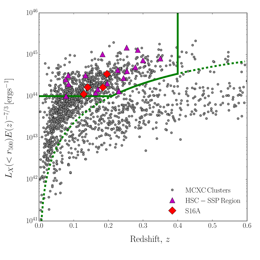
Figure 1: Target selection: X-ray luminosity versus redshift for the MCXC clusters based on the ROSAT all sky survey. The green solid lines indicate our sample selection. The green dotted line is a flux threshold of $10^{-12}~{}{\rm erg~{}s^{-1}cm^{-2}}$. Red diamonds and magenta triangles denote the targeting clusters in the paper and the full area ($\sim 1400$ deg²) of the HSC-SSP survey, respectively.

Table 1: Cluster sample: ^a Cluster name. ^b Alternative name. ^c Cluster redshift from the MCXC catalog. ^d X-ray centroid. ^e BCG position. ^f The center of CAMIRA catalog. ^g Cluster optical richness. ^h WL mass measurement satisfying the the full-depth and full-colour conditions for the current HSC-SSP footprint. ^† We retrieved the data from the CAMIRA catalog (Oguri et al. 2017).

Namea	Alternative nameb	redshiftc	$(\alpha,\delta)_{\rm xmm}^{d}$	$(\alpha,\delta)_{\rm bcg}^{e\dagger}$	$(\alpha,\delta)_{\rm camira}^{f\dagger}$	$N_{\rm cor}^{g\dagger}$	WLh
MCXCJ0157.4-0550	ABELL 281	0.12890	(29.294, -5.869)	(29.279, -5.887)	(29.301, -5.918)	41.3	no
MCXCJ0231.7-0451	ABELL 362	0.18430	(37.927, -4.882)	(37.922, -4.882)	(37.922, -4.883)	116.4	yes
MCXCJ0201.7-0212	ABELL 291	0.19600	(30.429, -2.196)	(30.430, -2.197)	(30.445, -2.198)	76.2	no
MCXCJ1415.2-0030	ABELL 1882A	0.14030	(213.785, -0.491)	(213.785, -0.494)	(213.785, -0.493)	43.0	yes
MCXCJ1415.2-0030W	ABELL 1882B	0.14400†	(213.601, -0.377)	(213.600, -0.379)	(213.618, -0.330)	68.8	yes

3 X-ray Analysis

In order to measure the total cluster mass with X-rays from the ICM gas, which is assumed to be in H.E. with the cluster gravitational potential, we need the gas density and temperature profiles. European Photo Imaging Camera (EPIC; Turner et al. 2001; Strüder et al. 2001) on board the XMM-Newton satellite offers an opportunity to perform extremely sensitive imaging/spectroscopic observations for clusters. EPIC data were analyzed with the ESAS (Extended Source Analysis Software) package (Snowden et al. 2008). The details of the data analysis are described in the following sections. In this work, we used SAS version 16.0.0 and HEAsoft version 6.19 with the latest CALDB as of November 2016.

3.1 Data reduction

The EPIC data were processed and screened in the standard way by using the ESAS pipeline. The data were filtered for intervals of high background due to soft proton flares, defined to be periods when the rates were out of the $2\sigma$ range of a rate distribution. Point sources are removed from three EPIC (MOS1, MOS2, and pn) images with simultaneous maximum likelihood PSF fitting. The radius to mask a point source is chosen so that the surface brightness of the point source is one quarter of the surrounding background. If the radius is less than half of the power diameter (HPD$\sim 15^{\prime\prime}$), we reset the radius to HPD. Table 2 summarizes the cluster data observed with XMM-Newton.

Table 2: X-ray data in the S16A field. ^aCluster name. ^bObservational ids. ^c Net exposure time of each instrument after the data reduction. ^†Data observed through our program. ^♮ Archival data.

Namea	obsidb	Net exposure (ks)c
		MOS1	MOS2	pn
MCXCJ0157.4-0550	0781200101†	27.8	27.2	16.1
MCXCJ0231.7-0451	0762870201†	22.5	22.3	15.5
MCXCJ0201.7-0212	0655343801♮	22.4	22.4	14.9
MCXCJ1415.2-0030	0762870501†	19.3	19.0	13.0
MCXCJ1415.2-0030W	0145480101♮	11.0	11.7	7.0

3.2 Spectral fit

In order to determine the gas temperature profile, a spectral fit is performed in the same way as in Snowden et al. (2008), where all spectra extracted from regions of interest are simultaneously fitted with a common model, including particle and cosmic background components which are assumed to be uniform across the detector except for instrumental lines. In this work, we used all three EPIC instruments of the MOS1,MOS2 and pn cameras. Three spectra, one from each instrument, are extracted from concentric annuli centered on an intensity-weighted centroid of the cluster. As for the intensity-weighted centroid, we first select an intensity peak and then iteratively determine intensity-weighted centroids. within the radius of $500~{}h_{70}^{-1}$ kpc from the centroid. At each iteration, we exclude regions, of which sizes are the same as those of the excluded point sources (Sec. 3.1), at their axially symmetric positions with respect to the centroid computed by the previous iteration. This process is important in order to avoid central shifts by the excluded point sources. The calculation is converged within several iterations. Each spectrum is binned in energy to have at least 35 counts per spectral bin including background. Since the finite PSF effect can not be ignored for spectral fits of cluster diffuse emission, we consider contaminations from surrounding annuli using cross-talk auxiliary response files (ARFs) in the spectral fitting. The cross-talk contribution to the spectrum in a given annulus from a surrounding annulus is handled as an additional model component.

The instrumental background spectrum, which is stable with time, is modeled with data acquired with the filter wheel closed, available in ESAS CALDB, and is subtracted from the observed spectrum. The other particle backgrounds consisting of a continuum produced by soft protons and instrumental lines are determined by adding a power-law spectrum and narrow Gaussian lines with fixed central energies to the fitting model, respectively. The power-law model representing the soft proton background is added only in MCXCJ0157.4-0550 because, for the other clusters, the spectrum in the outermost region of interest is not affected by the contamination of the soft proton background and therefore corresponding model is negligible.

The cosmic diffuse background consists of cosmic X-ray background (CXB), Galactic diffuse emission, and solar wind charge exchange (SWCX) emission lines, all of which are added to the fitting model. The CXB component is modeled with a power-law spectrum with a fixed index of 1.46 according to Snowden et al. (2008). The Galactic diffuse emission is fitted with the sum of absorbed and non-absorbed thermal plasma emission models, with the temperature ranging from 0.25 to 0.7 keV and from 0.1 to 0.3 keV, respectively. The SWCX lines are two narrow Gaussian models with fixed central energies of 0.56 and 0.65 keV, which correspond to OVII and OVIII lines, respectively. The CXB and Galactic diffuse emission are constrained by simultaneously fitting a spectrum extracted from the $1^{\circ}$–$2^{\circ}$ annulus region surrounding the cluster using the ROSAT all sky survey (RASS) data (Snowden et al. 1997).

The ICM emission spectrum is fitted by a thermal plasma emission model, APEC (Smith et al. 2001), with the Galactic photoelectric absorption model, phabs (Balucinska-Church & McCammon 1992). In the identical annuli of the three EPIC detectors, each spectrum has common model parameters for ICM emission except for a normalization factor for cross-calibration. The metal abundance relative to solar from Anders & Grevesse (1989) in each annulus is co-varied among the three instruments. When the metallicity at large radii is not constrained, it is the same as the value determined in the adjacent inner annulus. The power-law indices of the soft proton background are different free parameters in the MOS and pn, but are common in all annuli for each detector. The normalization for the soft proton background in individual annuli varies according to a scale factor computed from ESAS CALDB which contains actual soft proton events (see Fig.4 in Snowden et al. 2008). Cluster redshift, the hydrogen column density for the Galactic absorption, and instrumental line center energies are also common but fixed. The hydrogen column densities use weighted averages from Kalberla et al. (2005) at cluster positions.

To properly treat the finite size of the PSF in XMM-Newton affect, we considered cross-talk ARFs (Snowden et al. 2008) of neighboring three or less annuli in the spectral fit. A change of best-fit temperatures derived with and without cross-talk ARFs occurs at very central region of which radial width is $\sim 1^{\prime}$. We summarize the result of the spectral-fit in Appendix A and Table 4. Figure 2 is a typical spectrum of MOS1 in the center region of MCXCJ0157.4-0550.

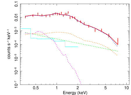
Figure 2: Observed MOS1 spectrum in the center region of MCXCJ0157.4-0550 with various fitting model components. In the actual fitting, all 24 spectra are jointly fitted with the common model. The red points show the observed spectrum with the instrumental background subtracted. The red solid line is the sum of all components. The blue, magenta, orange and green dotted lines are the thermal emission spectrum of the cluster, Galactic diffuse emission, CXB, and the residual soft proton component, respectively. The light blue line is the RASS spectrum.

3.3 Surface brightness profile

The X-ray surface brightness profiles over entire detector regions are derived from the 0.4–2.3 keV image, from which the instrumental background is already subtracted. We assume that the surface brightness profile follows a linear combination of $\beta$ models (Cavaliere & Fusco-Femiano 1976; Jones & Forman 1984), to analytically describe multi-scale and/or multi-component of the X-ray emitting gas. The model profile is described as follows,

$$S_{X}^{\rm tot}(R)=\sum_{i=1}^{n}S_{X,i}(R)+B$$ (1)

where $S_{X,i}$ is a single $\beta$ model,

$$S_{X}(R)=S_{0}\left(1+\left(R/r_{c}\right)^{2}\right)^{1/2-3\beta},$$ (2)

and $R$ is the projected distance from the center and $B$ is a constant offset representing the CXB of each instrument. We monitor whether the best-fit $B$s are in good agreement with the blank sky. We confirmed that the surface brightness in the target fields and blank sky are fairly constant at radii where the CXB dominates. The $\beta$ model is convolved with each corresponding instrument point spread function (PSF) and is simultaneously fitted to the corresponding surface brightness profile of all three EPIC detectors; $\chi^{2}=\chi^{2}_{\rm MOS1}+\chi^{2}_{\rm MOS2}+\chi^{2}_{\rm pn}$. We first fit the $\beta$ model to the data and, if it yields an apparent poor fit, we add another component to the model. All our data can be well expressed by $n\leq 2$. Given the best-fit parameters, we can decompose the three dimensional density profile with a linear combination,

$$n_{i}^{2}(r)=n_{0,i}^{2}\left(1+\left(r/r_{c,i}\right)^{2}\right)^{-3\beta_{i}}.$$ (3)

Here, $r$ is the three-dimensional distance from the center. We compute the emissivity in the given energy band from the best-fit parameters of spectral analysis and conversion factors between $S_{X}$ and $n_{e}$ considering detector sensitivities. The surface brightness is in general measured over larger radii than that for spectral analysis, and the conversion factor at large radii is extrapolated with a linear function of the radius. If we convert using the central emissivity only, the electron number density is underestimated by $\sim 10\%$ at $\sim r_{500}$.

To fairly model multiple components for an internal substructure in MCXCJ0157.4-0550 (Section 6.1; Figures 3 and 4) and a contamination from the close-pair cluster, MCXCJ1415.2-0030 and MCXCJ1415.2-0030W (Section 6.4), we take into account X-ray emission from gas components offset from the main cluster when determining the surface brightness. The off-centering effect in the surface brightness is calculated by

$$S_{\rm X,off}(R)=\frac{1}{2\pi}\int_{0}^{2\pi}d\theta S_{\rm X}(\sqrt{R^{2}+d_{\rm off}^{2}-2Rd_{\rm off}\cos\theta}).$$ (4)

Here $d_{\rm off}$ is the off-centering distance on the sky. When we model without the off-centering effect, the outer slope $\beta$ is misestimated and the H.E. mass estimates are biased. As a sanity check, we compute the surface brightness profiles excluding the area within which the best-fit number density for the off-centered component is more than $10^{-2}$ of its central density and confirm that the best-fit results do not change.

3.4 Temperature profile

The temperature profile is modeled with a generalized universal profile (Martino et al. 2014; Okabe et al. 2014b),

$$T_{\rm 3D}(r)=T_{0}\frac{(r/r_{t})^{a}}{(1+(r/r_{t})^{2})^{c/2}}.$$ (5)

The temperature profile projected along the line-of-sight is estimated with a weight $w$,

$$T_{\rm 2D}=\frac{\int T_{\rm 3D}wdV}{\int wdV},$$ (6)

in each annulus. We here assume the spectroscopic-like temperature (Mazzotta et al. 2004; Martino et al. 2014) with $w=n^{2}T_{3D}^{-3/4}$. When the low photon-statistics prevents us from constraining a temperature profile, we assume the inner slope $a=0$ and/or the outer slope $c=1$, following an universal temperature profile out to $r_{200}$ based on joint Subaru WL and Suzaku X-ray analysis (Okabe et al. 2014b). We also assume a constant profile for MCXCJ1415.2-0030W because the temperatures are measured only in two annuli. The measurement uncertainty for the number density is also propagated to the temperature fitting.

3.5 H.E. Mass profile

Given the best-fit parameters, the three-dimensional spherical total mass is estimated with the H.E. assumption,

$$M_{\rm H.E.}(r)=-\frac{k_{B}T_{\rm 3D}(r)r}{\mu m_{p}G}\left[\frac{d\ln\rho_{g}(r)}{d\ln r}+\frac{d\ln T_{\rm 3D}(r)}{d\ln r}\right],$$ (7)

where $\mu=0.5964$ is the mean molecular weight for the metallicity $Z=0.3$ and $\rho_{g}=1.9257\mu n_{e}m_{p}$ is the gas density profile. Here, $n_{e}$ is the electron density and $m_{p}$ is the proton mass. We then estimated the total mass, $M_{500}$, within $r_{500}$ and the spherical gas mass, $M_{\rm gas}(r)$, calculated by integrating $\rho_{g}$ out to the radius, $r_{500}$.

Table 3: H.E. mass, WL mass, gas mass and stellar mass estimations at $\Delta=500$. Gas and stellar masses are enclosed within $r_{500}$ derived from H.E. masses.

Name	$M_{500}^{\rm H.E.}$	$M_{500}^{\rm WL}$	$M_{\rm gas}(<r_{500}^{\rm H.E.})$	$M_{*}(<r_{500}^{\rm H.E.})$
	($10^{14}\mathrel{h_{70}^{-1}M_{\odot}}$)	($10^{14}\mathrel{h_{70}^{-1}M_{\odot}}$)	($10^{13}h_{70}^{-5/2}M_{\odot}$)	($10^{12}h_{70}^{-2}M_{\odot}$)
MCXCJ0157.4-0550	$1.37_{-0.08}^{+0.09}$	-	$2.12_{-0.11}^{+0.12}$	$2.63_{-0.05}^{+0.05}$
MCXCJ0231.7-0451	$3.43_{-0.65}^{+0.77}$	$7.96_{-1.89}^{+2.58}$	$4.39_{-0.40}^{+0.42}$	$8.87_{-0.34}^{+0.31}$
MCXCJ0201.7-0212	$3.21_{-0.44}^{+0.51}$	-	$4.28_{-0.30}^{+0.32}$	$5.75_{-0.16}^{+0.15}$
MCXCJ1415.2-0030	$1.54_{-0.23}^{+0.34}$	$2.09_{-0.90}^{+1.43}$	$1.08_{-0.12}^{+0.16}$	$5.39_{-0.18}^{+0.23}$
MCXCJ1415.2-0030W	$0.44^{+0.07}_{-0.07}$	$0.80_{-0.58}^{+0.87}$	$0.60_{-0.15}^{+0.17}$	$3.78_{-0.44}^{+0.37}$

4 Optical Catalog

We retrieved the cluster richness, $N_{\rm cor}$, and the stellar masses, $M_{*}$, from the CAMIRA cluster catalog (Oguri et al. 2017) which is constructed using the HSC-SSP Wide S16A data. The CAMIRA algorithm makes use of a stellar population synthesis model to predict colours of red sequence galaxies at a given redshift for an arbitrary set of bandpass filters and a three dimensional richness map with a compensated spatial filter. The details of the CAMIRA cluster algorithm are described in Oguri (2014) and Oguri et al. (2017). The smoothing scale for the compensated spatial filter is $R_{0}=0.8h^{-1}{\rm Mpc}$ in physical units. The total stellar mass for red galaxies of each cluster is estimated by convolution with the spatial filter. Since blue galaxies are a subdominant component in stellar mass at low redshifts, we estimate the stellar mass only using red galaxies. We confirmed that the photometric redshifts provided by the CAMIRA cluster catalog excellently agree with the spectroscopic redshifts.

We here use the stellar masses rather than optical luminosities because the HSC-SSP multi-band datasets are capable of estimating the stellar masses (Oguri et al. 2017). Following Miyazaki et al. (2015), we convert the total stellar masses ($M_{*}^{\rm CAMIRA}$) of each CAMIRA cluster into one enclosed within a measurement radius ($M_{*}(<r_{\Delta})$) . The conversion factor, $A\equiv M_{*}(<r_{\Delta})/M_{*}^{\rm CAMIRA}$, can be calculated as follows. We first assume that the stellar mass density profile is described by a universal mass density profile (Navarro et al. 1996, 1997, hereafter NFW) with the mass and concentration relation of Diemer & Kravtsov (2014) with the Planck cosmology (Planck Collaboration 2015). Here, the NFW profile is expressed in the form:

$$\rho_{\rm NFW}(r)=\frac{\rho_{s}}{(r/r_{s})(1+r/r_{s})^{2}},$$ (8)

where $\rho_{s}$ is the central density parameter and $r_{s}$ is the scale radius. The halo concentration is defined by $c_{\Delta}=r_{\Delta}/r_{s}$, where $r_{\Delta}$ is the overdensity radius. Given the mass and its assumed concentration, the conversion factor, $A$, is obtained as the ratio derived by integrating the projected NFW profile out to the measurement radius and to infinity, with a convolution of the spatial filter. When a measurement center is offset from the CAMIRA center, we calculate the azimuthally averaged, projected NFW density around the measurement center and then integrate it out to the measurement radius in a similar manner to the equation 4. As mentioned in Miyazaki et al. (2015), this correction technique takes into account the three dimensional deprojection. We measure stellar masses at $\Delta=500$ derived by X-ray mass measurements and estimate gas and baryon fractions with the X-ray gas measurements (Section 6.7). Some very luminous galaxies in clusters are missed by flags in the CAMIRA catalog because their luminosity cannot be accurately measured due to saturation. If an offset between the CAMIRA and X-ray centers are large, the number of missing luminous galaxies is relatively large. To include missing luminous galaxies, we add stellar masses of luminous member galaxies identified by SDSS spectroscopic observations. The stellar masses and gas fractions including the luminous galaxies are $\sim 3-47\%$ and $\lower 2.15277pt\hbox{$\;\buildrel<\over{\sim}\;$}14\%$ higher, respectively.

5 Weak-lensing Mass Measurement

We carry out WL analysis using the WL shear data estimated by re-Gaussianization method (Hirata & Seljak 2003) which is implemented in the HSC pipeline (see details in Mandelbaum et al. 2017a). Both precise shape measurement and photometric redshift estimation are essential for the WL related studies, which offers the strict conditions on the depth of data and the availability of five-band photometry. For this reason, the WL shear catalog is restricted to the full-depth and full-colour footprint. Three out of five clusters are located in the those regions, namely, MCXCJ0231.7-0451, MCXCJ1415.2-0030 and MCXCJ1415.2-0030W, for which we measure WL masses (Table 1).

In cluster lensing, a contamination of unlensed member galaxies in the source catalog significantly underestimates lensing signals at small radii, because the fraction of member and background galaxies is increasing with decreasing radius. It is known as the dilution effect (Broadhurst et al. 2005). Previous studies (e.g. Okabe et al. 2013, 2014b; Okabe & Smith 2016) have shown that if there is no background selection, lensing signals for massive clusters at $z\sim 0.2$ are underestimated by $\sim 40\%$. Previous studies (Okabe et al. 2013; Okabe & Smith 2016; Medezinski et al. 2010, 2015; Umetsu et al. 2016) securely selected background galaxies using colour information and succeeded in keeping the level of contamination below a few percent. We here briefly summarize the method. It is very difficult to discriminate between faint members and background galaxies by magnitude information because of large photometric uncertainty and the intrinsic scatter of color distribution. We select a colour space region in which member galaxies are negligible by monitoring a consistency among three independent information of colour, lensing signal and available, external photometric redshift catalog (Ilbert et al. 2013). Since passively-evolving member galaxies are localized in colour space, the mean tangential distortion strength in the colour space close to the red sequence is significantly underestimated because member galaxies are not lensed. However, the mean lensing signals, which are computed by the ensemble shear and the photometric redshift, outside of red-sequence color-space are flatten due to a reduction in contamination by member galaxies. By modeling the colour distribution of faint member galaxies, we have succeed in keeping the contamination limit at less than a few $\%$. In this procedure, we considered both shape noises and errors of photometric redshifts.

Based on a similar philosophy, Medezinski et al. (2017) have developed a new scheme to make a secure selection of background galaxies. We utilized lensing signals and four-band magnitudes ($griz$) of the HSC-SSP survey, internal photometric redshifts (Tanaka et al. 2017) computed by machine learning (MLZ; Carrasco Kind & Brunner 2014) calibrated with spectroscopic data. We have succeeded in selecting background galaxies in the $rz$ and $gi$ colour plane as the best combination for the HSC-SSP survey. Based on Medezinski et al. (2017, see for details), we select background galaxies for WL mass measurements (see also Miyatake et al. in prep). The number of background galaxies after the color cuts is $\lower 2.15277pt\hbox{$\;\buildrel<\over{\sim}\;$}11\,{\rm arcmin}^{-2}$.

Given the shape catalog of background galaxies, we measure the reduced tangential shear $\langle\Delta\Sigma_{+}\rangle(r_{i})$ computed by azimuthally averaging the measured galaxy ellipticity, $e_{\alpha}$ ($\alpha=1,2$), for $n$-th galaxy in a given $i$-th annulus ($r_{\rm inn}<r_{i}<r_{\rm out})$, centering at the brightest cluster galaxies (BCGs),

$$\langle\Delta\Sigma_{+}\rangle(r_{i})=\frac{\sum_{n}e_{+,n}w_{n}\langle\Sigma_{{\rm cr},n}^{-1}\rangle^{-1}}{2{\mathcal{R}}_{i}(1+K_{i})\sum_{n}w_{n}},$$ (9)

where the tangential ellipticity is

$$e_{+} = -(e_{1}\cos 2\varphi+e_{2}\sin 2\varphi),$$ (10)

and the inverse of the mean critical surface mass density ($\langle\Sigma_{{\rm cr}}^{-1}\rangle$), the weighting function ($w_{n}$), the shear responsivity (${\mathcal{R}}$), and the calibration factor ($K$) are defined below. The inverse of the mean critical surface mass density is computed by the probability function $P(z)$ of the MLZ photometric redshift,

$$\langle\Sigma_{{\rm cr}}^{-1}\rangle=\frac{\int^{\infty}_{z_{l}}\hat{\Sigma}_{{\rm cr}}^{-1}(z_{l},z_{s})P(z_{s})dz_{s}}{\int^{\infty}_{0}P(z_{s})dz_{s}}.$$ (11)

Here, $z_{l}$ and $z_{s}$ are the cluster and source redshift, respectively. The critical surface mass density for individual background galaxies is expressed by $\hat{\Sigma}_{{\rm cr}}=c^{2}D_{s}/4\pi GD_{l}D_{ls}$, where $D_{s}$, $D_{l}$ and $D_{ls}$ are the angular diameter distances from the observer to the sources, from the observer to the lens, and from the lens to the sources, respectively. Since $\hat{\Sigma}_{\rm cr}$ becomes zero for $z_{s}<z_{l}$, the lower bound of the integration is truncated by $z_{l}$. The weighting function $w_{n}$ is given by

$$w_{n}=\frac{1}{e_{{\rm rms},n}^{2}+\sigma_{e,n}^{2}}\langle\Sigma_{{\rm cr},n}^{-1}\rangle^{2},$$ (12)

where $e_{\rm rms}$ and $\sigma_{e}$ are the root mean square of intrinsic ellipticity and the measurement error per component ($\alpha=1$ or $2$), respectively. Here, the intrinsic ellipticity expresses the ellipticity for the intrinsic shape of galaxies. The shear responsivity is computed based on the ellipticity definition,

$${\mathcal{R}_{i}}=1-\frac{\sum_{n}e_{\rm rms,n}^{2}w_{n}}{\sum_{n}w_{n}},$$ (13)

(see also Mandelbaum et al. 2005; Reyes et al. 2012). We correct the measured values using the shear calibration factor $(m,c)$ for individual objects (Mandelbaum et al. 2017a), because of systematic error of shape measurements. The measured ensemble shear, $\langle\gamma\rangle$, can be expressed by $(1+m)\gamma_{\rm true}+c$ with the input shear $\gamma_{\rm true}$, as defined by STEP (Shear TEsting Programme) simulations (Heymans et al. 2006; Massey et al. 2007). Here, a multiplicative calibration bias $m$ and an additive residual shear offset $c$ are estimated based on GREAT3-like simulations (Mandelbaum et al. 2017b, 2014, 2015) as a part of the GREAT (GRavitational lEnsing Accuracy Testing) project. The calibration factor, $K$, is computed by

$$K_{i}=\frac{\sum_{n}m_{n}w_{n}}{\sum_{n}w_{n}}.$$ (14)

We also conservatively subtract

$$\tilde{c}_{i}=\frac{\sum_{n}c_{+,n}w_{n}\langle\Sigma_{{\rm cr},n}^{-1}\rangle^{-1}}{(1+K)\sum_{n}w_{n}}$$ (15)

from $\langle\Delta\Sigma_{+}\rangle(r_{i})$ (equation 9). The additional offset term is negligible ${\mathcal{O}}(<10^{-4})$ compared to $\langle\Delta\Sigma_{+}\rangle\sim{\mathcal{O}}(10^{-1})$.

Following Okabe & Smith (2016), we employ a maximum-likelihood method to model the shear profiles, and express the log-likelihood as follows:

$$-2\ln{\mathcal{L}} = \ln(\det(C_{ij}))+$$

$$\sum_{i,j}(\Delta\Sigma_{+,i}-f_{{\rm model}}(r_{i}))C_{ij}^{-1}(\Delta\Sigma_{+,j}-f_{{\rm model}}(r_{j})),$$

where the subscripts $i$ and $j$ are for the $i-$ and $j-$th radial bins, respectively. We adopt that $r_{i}$ is the weighted harmonic mean radius of the background galaxies. Here, $f_{\rm model}$ is the reduced shear prediction for a specific mass model,

$$f_{{\rm model}}(r_{i})=\frac{\Delta\tilde{\Sigma}_{\rm model}(r_{i})}{1-{\mathcal{L}}_{z,i}\Sigma_{\rm model}(r_{i}))},$$ (17)

with $\Delta\tilde{\Sigma}_{\rm model}=\gamma_{+}\langle\Sigma_{\rm cr,n}^{-1}\rangle^{-1}$ and $\Sigma_{\rm model}=\kappa\langle\Sigma_{\rm cr,n}^{-1}\rangle^{-1}$. Here, $\gamma_{+}$ is the dimensionless tangential shear and $\kappa$ is the convergence, respectively. The covariance matrix, $C=C_{g}+C_{s}+C_{\rm LSS}$, in equation 5 is composed of the shape noise $C_{g}$, the uncertainty of source redshift $C_{s}$ and the photometric redshift error computed by $P(z)$ and uncorrelated large-scale structure (LSS), $C_{\rm LSS}$, along the line-of-sight (Schneider et al. 1998). The covariance matrix for shape noise is obtained as weighted variance

$$C_{g,ij}=\left(\frac{1}{4R_{i}^{2}(1+K_{i})^{2}\sum w_{n}}\right)\delta_{ij},$$ (18)

where $\delta_{ij}$ is a kronecker delta function. The photometric error for individual galaxies is estimated by

$$\delta\langle\Sigma_{{\rm cr}}^{-1}\rangle=\frac{\int^{\infty}_{z_{l}}(\hat{\Sigma}_{{\rm cr}}^{-1}(z_{l},z_{s})-\langle\Sigma_{{\rm cr}}^{-1}\rangle)^{2}P(z_{s})dz_{s}}{\int^{\infty}_{0}P(z_{s})dz_{s}},$$ (19)

and then we propagate it into the measurement as $C_{s}$. The covariance matrix, $C_{\rm LSS}$, is given by

$$C_{{\rm LSS},ij}=\langle\Sigma_{{\rm cr},i}^{-1}\rangle^{-1}\langle\Sigma_{{\rm cr},j}^{-1}\rangle^{-1}\int\frac{ldl}{2\pi}P_{\kappa}(l)J_{2}(l\theta_{i})J_{2}(l\theta_{j}),$$ (20)

where $P_{\kappa}(l)$ is the weak-lensing power spectrum (e.g. Schneider et al. 1998; Hoekstra 2003), calculated by multipole $l$, the source redshift, and a given cosmology. We employ the Planck cosmology (Planck Collaboration 2015) for $\Omega_{b0}$, $\sigma_{8}$ and the spectral index $n_{s}$. Here, $J_{2}(l\theta_{i})$ is the Bessel function of the first kind and second order at the $i$-th annulus (Hoekstra 2003).

The source redshift at each radial bin are calculated from lensing-efficiency weighted value, as follows

$${\mathcal{L}}_{z,i}=\frac{\sum_{n}\langle\Sigma_{\rm cr,n}^{-1}\rangle w_{n}}{\sum_{n}w_{n}}.$$ (21)

Following numerical simulations (Navarro et al. 1996) and previous observational results (e.g. Okabe et al. 2013, 2016; Oguri et al. 2012; Umetsu et al. 2016), we adopt the NFW profile (Navarro et al. 1996) as the mass model. Similar to the X-ray analysis, we define the three-dimensional spherical mass, $M_{500}$, enclosed by the radius, $r_{500}$. We basically fit for two parameters : the mass and the halo concentration. The resulting masses are shown in Table 3.

6 Results and Discussion

We carried out X-ray analysis and joint X-ray and optical analysis for the four MCXC clusters and the non-MCXC cluster (Table 1) in the current coverage region for the HSC-SSP survey. As mentioned in Section 5, the sample for WL mass measurement is only the three clusters (Table 1) due to the full-colour and full-depth conditions. Thus, we shall use the WL mass estimates only for X-ray and WL mass comparisons.

Since this paper is a sort of pilot studies to directly compare multi-wavelength datasets, we shall first discuss results for individual clusters based on both X-ray and optical datasets. We then perform studies of a correlation between H.E. masses and richness, a mass comparison and baryon fraction for the current sample of clusters.

6.1 MCXCJ0157.4-0550

MCXCJ0157.4-0550 is an on-going cluster merger at $z=0.1289$ as shown in Figure 4. The system is composed of the western main gas halo and the northeast subhalo. Optically-luminous galaxies are concentrated in the western region where the X-ray morphology is highly elongated along the west-east direction. The CAMIRA center is slightly offset from both X-ray and the BCG centers, because some luminous galaxies are missing in the HSC CAMIRA catalog. A comma-shaped feature in the X-ray emission is discovered at $\sim 1.6r_{500}\sim r_{200}$ ( $r_{200}$ based on H.E. mass estimation (Section 3.5)), which suggests ram pressure stripping of the sub-cluster. An optically-luminous galaxy is located at the sub-cluster X-ray peak. The redshift retrieved from the SDSS, $0.1286$, is very close to the cluster redshift, suggesting that the substructure is infalling in the plane of the sky. It is consistent with the fact that a prominent tail is observed. The comma-shaped feature also implies that the infalling gas observed in the X-ray has large angular-momentum. If we improperly treat the substructure in the X-ray surface brightness ($S_{x}$) modeling, it may change the outer density slope (Equation 2) of the main halo and eventually affect the H.E. mass estimation. Furthermore, we cannot rule out a possibility that the slopes in the disturbed (east) and undisturbed (west) sectors are different. Since our analysis measures azimuthally-averaged X-ray quantities to estimate spherical H.E. masses under the assumption of spherical symmetry, it is not good to divide into azimuthally-dependent sub-sectors in order to estimate the azimuthally-averaged outer slope. To solve these problems, we implement the subtraction using the off-centering effect (Equation 4) in a model of the azimuthally averaged surface brightness profile centering the western gas halo. As a first approximation, we assume the $\beta$ model for the western main gas halo and the northeast subhalo. The resulting profile well describes the observed surface brightness (Figure 3).

The H.E. mass is estimated only for the main cluster. The total gas mass within $\sim r_{200}$ computed for both the main gas and the gas substructure is $\sim 8\%$ higher than that estimated by the main cluster component, while the gas mass within $r_{500}$ does not change.

Unfortunately, this cluster is located outside of the full-depth and full-colour region of the HSC-SSP S16A data, and thus the WL shape data are not available. A mass comparison for this cluster will be carried out in a future study.

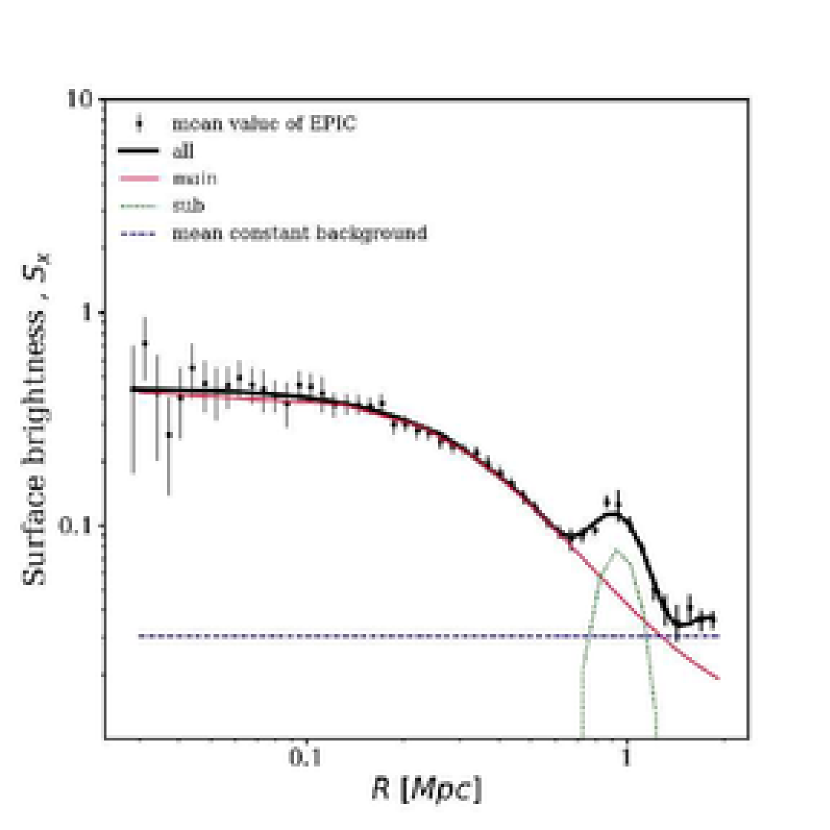
Figure 3: The X-ray surface brightness profile for MCXCJ0157.4-0550 in arbitrary units averaged over three instruments. The projected distance is described by $R$. The profile is corrected with different effective areas and background levels of MOS and pn. The center is the flux-weighted X-ray centroid of the western main cluster. Thin red solid, green dotted and blue dashed lines show the model profile of the western main cluster, the off-centered sub cluster and the mean constant background, respectively. The thick black solid line is the sum over all components, which describes the observed profile very well.

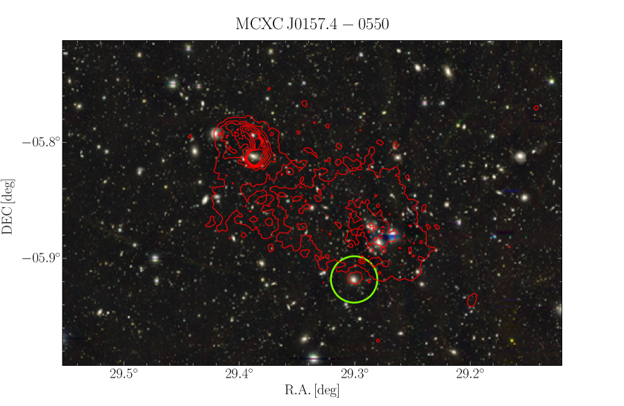
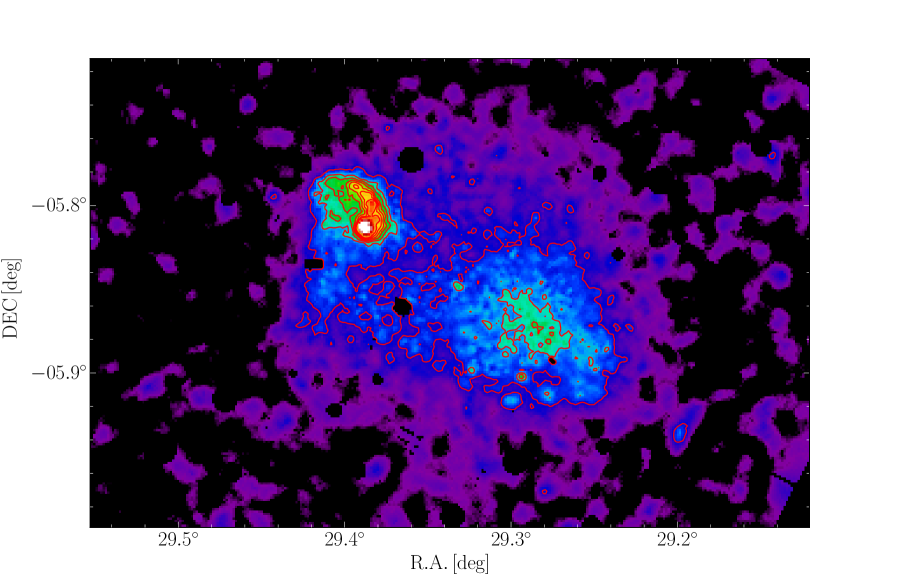
Figure 4: Left : HSC $gri$ pseudo colour image for MCXCJ0157.4-0550, overlaid with vignetting-corrected X-ray contours excluding point sources in red colour. The green circle has a $1.^{\prime}2$ radius and is centered on the CAMIRA cluster. The BCG is located at $(\alpha,\delta)=(29.279,-5.887)$. Right: Adaptively smoothed image in $0.4-2.3$keV excluding point sources. The contours with the vignetting correction are 7 levels linearly spaced from [10-100] ${\rm cts~{}s}^{-1}{\rm deg}^{-2}$. The northeast gas substructure clearly shows a comma-shaped feature, suggesting ram-pressure stripping.

6.2 MCXCJ0231.7-0451

We present new observations of the cluster ($z=0.1843$) located in the XXL survey region with XMM-Newton. An X-ray luminous point source at $\sim 3.^{\prime}5$ east of the X-ray center is found. Faint X-ray emission from another CAMIRA cluster at $z=0.2760$ is also detected around the edge of the X-ray detectors (Figure 5). These X-ray sources are excluded in our analysis.

The cluster is referred to as XXL091 in the XXL survey (Eckert et al. 2016), and has $M_{\rm gas}=5.00^{+0.80}_{-0.83}\times 10^{13}\mathrel{h_{70}^{-1}M_{\odot}}$ within $r_{500}^{\rm MT}=1149\pm 161h_{70}^{-1}{\rm kpc}$. Here, $r_{500}^{\rm MT}$ is derived from a scaling relation between WL mass and X-ray temperature (Lieu et al. 2016). We find that our measurement $M_{\rm gas}=5.10^{+0.85}_{-0.84}\times 10^{13}\mathrel{h_{70}^{-1}M_{\odot}}$ within the same radius is in good agreement with Eckert et al. (2016).

The mass estimation of the Planck SZ observation (Planck Collaboration et al. 2015) gives $M_{500}^{\rm SZ}=3.96^{+0.49}_{-0.49}\times 10^{14}\mathrel{h_{70}^{-1}M_{\odot}}$, which agrees with our H.E. mass estimate $M_{500}^{\rm H.E.}=3.43^{+0.77}_{-0.65}\times 10^{14}\mathrel{h_{70}^{-1}M_{\odot}}$.

Our WL mass measurement gives, $M_{500}^{\rm WL}=7.96_{-1.89}^{+2.58}\times 10^{14}\mathrel{h_{70}^{-1}M_{\odot}}$, which agrees within errors with the CFHT WL mass measurement $M_{500}^{{\rm WL}}=6.2^{+2.1}_{-1.8}\times 10^{14}\mathrel{h_{70}^{-1}M_{\odot}}$ (Lieu et al. 2016).

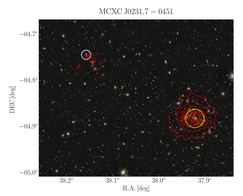
Figure 5: Optical image of MCXCJ0231.7-0451, overlaid with vignetting-corrected X-ray contours in red colour. Green circles show $1.^{\prime}2$ radius centering CAMIRA clusters. The western diffuse X-ray emission is from the target cluster. Faint X-ray emission from another CAMIRA cluster with $N_{\rm cor}=33.70$ at ($29.203,-6.119$) and $z=0.2760$, marked by a light-blue circle with $0.^{\prime}6$ radii, is also detected around the edges of the instruments. The contours with the vignetting correction are 7 levels linearly spaced from [10-100] ${\rm cts~{}s}^{-1}{\rm deg}^{-2}$.

6.3 MCXCJ0201.7-0212

This cluster is known as Abell 291, and has a cool core (Okabe et al. 2010, 2016; Martino et al. 2014). Since the HSC-SSP S16A data of the cluster do not satisfy the full-depth and full-colour conditions for WL mass measurement, we carry out X-ray and optical analysis.

We analyzed the same X-ray data used in Martino et al. (2014). The gas density profile is well described by a double $\beta$ model. The CAMIRA center is slightly offset from the X-ray centroid and the BCG (Figure 6), because a few bright galaxies are missing in the CAMIRA catalog. Our H.E. mass estimate, $M_{500}^{\rm H.E.}=3.21_{-0.44}^{+0.51}\times 10^{14}\mathrel{h_{70}^{-1}M_{\odot}}$, agrees with a previous X-ray study $M_{500}=2.92\pm 0.56\times 10^{14}\mathrel{h_{70}^{-1}M_{\odot}}$ (Martino et al. 2014). These H.E. mass estimates are slightly lower than the corresponding estimated WL mass $M_{500}^{\rm WL}=4.46^{+1.01}_{-0.96}\times 10^{14}\mathrel{h_{70}^{-1}M_{\odot}}$ (Okabe & Smith 2016), but the difference is not statistically significant. A mass comparison using the HSC-SSP data is left for future works.

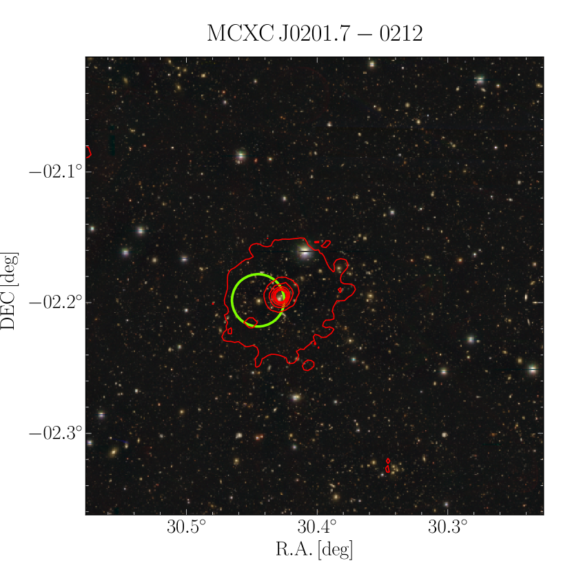
Figure 6: MCXCJ0201.7-0212. The colours are the same as those in Figure 4. The contours with the vignetting correction are 7 levels linearly spaced from [10-1000] ${\rm cts~{}s}^{-1}{\rm deg}^{-2}$.

6.4 MCXCJ1415.2-0030 and MCXCJ1415.2-0030W

The system is mainly composed of the originally-identified MCXC cluster, MCXCJ1415.2-0030, at the east and its companion cluster at $\sim 2$ Mpc northwest of the MCXC cluster. We refer to the western cluster as MCXCJ1415.2-0030W for convenience. The X-ray emission shows no evidence for disturbance due to merger activity. Besides the two clusters, two faint, diffuse X-ray emissions are found in the field (Figure 7). The northern emission $(\alpha,\delta)=(213.740,-0.350)$ and the north-western emission $(\alpha,\delta)=(213.541,-0.272)$ are associated with galaxies at $z=0.1389$ and $z=0.1398$, respectively. These components of which radii are $\sim 0.^{\prime}7-0.^{\prime}8$ are excluded in the following X-ray analysis. In the CAMIRA catalog, those galaxies are identified as a part of MCXCJ1415.2-0030W, giving a large richness. The X-ray emission from the eastern MCXC cluster coincides with the CAMIRA center, while the western emission is $\sim 3^{\prime}$ offset from the CAMIRA center. This is because the western CAMIRA cluster includes the northern and north-western groups. We find no evidence that the BCGs of the eastern and western clusters are significantly offset from the X-ray centroids. The X-ray luminosity of the eastern MCXC cluster is brighter than that of the western cluster, while the richness for the western cluster is higher. Owers et al. (2013, Figure 4 therein) have shown based on spectroscopic data that member galaxies of the eastern and western clusters are spread over $\sim 4$ Mpc and $\sim 1$ Mpc, respectively.

We analyzed X-ray data for these two clusters in order to measure gas temperatures and surface brightness profiles. To carefully estimate density outer-slopes, we computed two surface brightness profiles centering on each of the two clusters and simultaneously fit them with the two surface brightness models with the off-centering effect. We found that the observed profiles are well-described by the sum of X-ray emission of the two clusters, requiring no extra component such as a filamentary gas component bridge between the two clusters. In the surface brightness profile centered on MCXCJ1415.2-0030, the flux of the cluster, the other cluster and the background at $R\sim 1~{}{\rm Mpc}$ account for $\sim 1\%$, $\sim 13\%$ and $\sim 86\%$, respectively. In the temperature measurements for each cluster, we selected the background-dominated region for the annulus. Again, if we ignore the flux contamination from the other cluster in the surface brightness modelling, we overestimate the background component and eventually misestimate the outer slopes.

Based on the H.E. assumption, we estimate $M_{500}^{\rm H.E.}=1.54_{-0.23}^{+0.34}\times 10^{14}\mathrel{h_{70}^{-1}M_{\odot}}$ for MCXCJ1415.2-0030 and $M_{500}^{\rm H.E.}=0.44_{-0.07}^{+0.07}\times 10^{14}\mathrel{h_{70}^{-1}M_{\odot}}$ for MCXCJ1415.2-0030W (Table 3), respectively. It suggests that the originally-identified MCXC cluster is the main cluster.

We also carry out WL mass measurements for the two clusters. We adopt a maximum radius for each tangential shear profile centered on each BCG of $\sim 1.3h_{70}^{-1}$Mpc. Since the maximum radius is much less than the projected distance between the two clusters, the off-centering effect of lensing signal is negligible, $\sim{\mathcal{O}}(10^{-5})\times\langle\Sigma_{\rm cr}^{-1}\rangle^{-1}$ (Yang et al. 2006), in contrast to X-ray analysis. This is caused by the fact that $\Delta\Sigma_{+,\rm off}=\bar{\Sigma}_{\rm off}-{\Sigma}_{\rm off}$, where the the surface mass density for the off-centering component at the measured radius ($\Sigma_{\rm off}(R)$) is comparable to the mean surface mass density within the radius ($\bar{\Sigma}_{\rm off}(<R)$). The WL masses are $M_{500}^{\rm WL}=2.09_{-0.90}^{+1.43}\times 10^{14}\mathrel{h_{70}^{-1}M_{\odot}}$, for MCXCJ1415.2-0030 and $M_{500}^{\rm WL}=0.80_{-0.58}^{+0.87}\times 10^{14}\mathrel{h_{70}^{-1}M_{\odot}}$ MCXCJ1415.2-0030W (Table 3), respectively. Since the signal-to-noise ratio of the tangential shear profile for MCXCJ1415.2-0030W is small, we used one parameter, $M_{500}$, assuming the halo concentration based on the median value of the mass versus concentration relation (Diemer & Kravtsov 2014). A sum of best-fit viral radii $\sim 2.6~{}{\rm Mpc}$ is comparable to the projected separation $\sim 2~{}{\rm Mpc}$ and non-disturbed gas distribution, suggesting that the two clusters are at early phase of cluster merger. The H.E. mass for the western companion cluster is comparable to the WL mass.

Virial mass estimation (Owers et al. 2013) using spectroscopic data has shown that $M_{500}^{\rm vir}=1.5\pm 0.3\times 10^{14}\mathrel{h_{70}^{-1}M_{\odot}}$ for the main cluster (A1882A) and $M_{500}^{\rm vir}=1.0\pm 0.5\times 10^{14}\mathrel{h_{70}^{-1}M_{\odot}}$ for the companion cluster (A1882B), respectively. Dynamical mass estimates are in good agreement with our WL masses. Owers et al. (2013) also concluded based on joint X-ray and kinematics analysis that the system is likely to be before cluster merger. Our results agree with their conclusions.

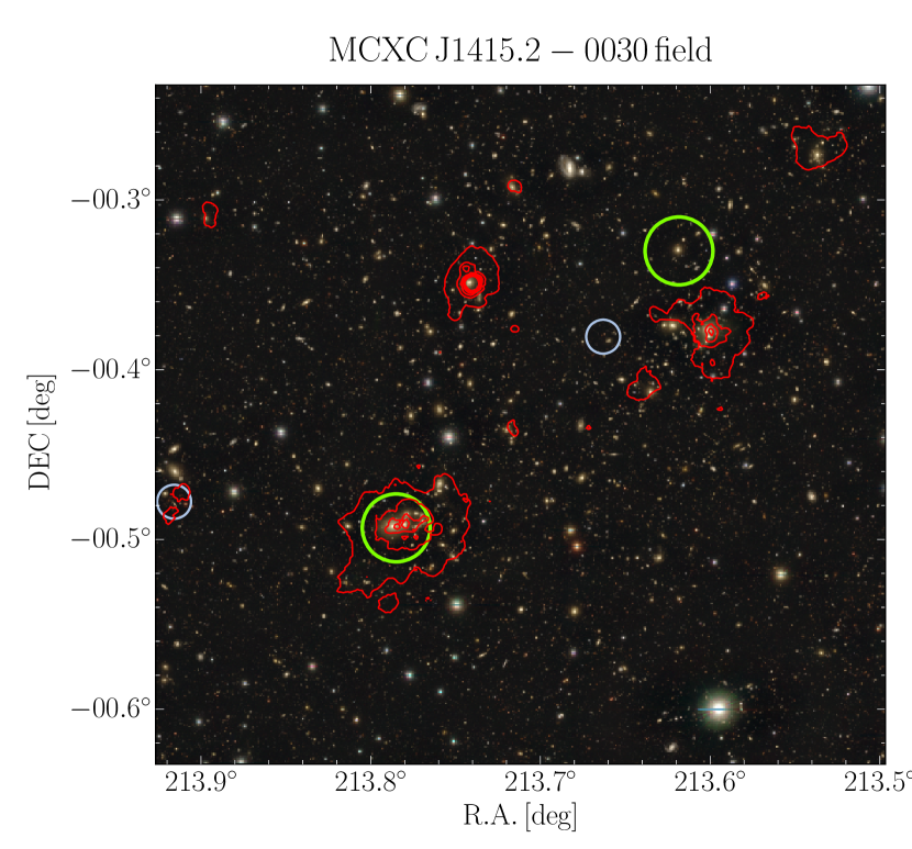
Figure 7: MCXCJ1415.2-003 field, overlaid with vignetting-corrected X-ray contours in red colour. Four diffuse X-ray sources are found in this field. MCXCJ1415.2-0030 and MCXCJ1415.2-0030W are at middle-left and middle-right of the panel, respectively. The other two diffuse X-ray emissions surrounding the system are found at $(\alpha,\delta)=(213.740,-0.350)$ and $(\alpha,\delta)=(213.541,-0.272)$. The green circles have a $1.^{\prime}2$ radius and are centered on the CAMIRA clusters. Two high-z CAMIRA clusters ($z>0.9$ and $N_{\rm cor}\lower 2.15277pt\hbox{$\;\buildrel>\over{\sim}\;$}15$) are found in the field, marked by light-blue circles with $0.^{\prime}6$ radii. The contours with the vignetting correction are 7 levels linearly spaced from [10-100] ${\rm cts~{}s}^{-1}{\rm deg}^{-2}$.

6.5 Richness vs $M_{\rm H.E.}$

We compare the H.E. masses for the MCXC clusters with the CAMIRA cluster richness. Since the cluster richness is generally proportional to the number of member galaxies, it is expected to be a good mass proxy. Indeed, Oguri et al. (2017) have compared public X-ray temperatures and luminosities in the XXL and XMM-LSS fields with their CAMIRA cluster richnesses, and found good correlations. The slope in the richness and temperature scaling relation (Oguri et al. 2017) is found to be shallower than that predicted by a self-similar solution. The temperatures are measured within a fixed radius, $300$ kpc, and thus are potentially and partially affected by baryonic physics. We here study a correlation between the H.E. masses and cluster richness.

Figure 8 compares the richness with the H.E. mass. The H.E. masses for the original sample of the MCXC clusters are $M_{500}\gtsim 1.5\times 10^{14}\mathrel{h_{70}^{-1}M_{\odot}}$, which is consistent with the masses we expected from choosing high luminosity clusters for this study, $M_{500}\gtsim 2\times 10^{14}\mathrel{h_{70}^{-1}M_{\odot}}$ (Section 2). A small discrepancy is acceptable when we consider intrinsic scatter in the scaling relation (Piffaretti et al. 2011). We fit the relation with a signal-power law model

$$\log\left(\frac{M_{500}^{\rm H.E.}}{10^{14}\mathrel{h_{70}^{-1}M_{\odot}}}\right)=a\log N_{\rm cor}+b$$ (22)

We here consider the relation consistent with our measurements for the four MCXC clusters and obtain $a=0.84\pm 0.15$ and $b=-2.73\pm 0.61$. The best-fit slope agrees with $\sim 1$ predicted by $N_{\rm cor}\propto M$ (Lin et al. 2004). The best-fit normalization suggests that $M_{500}^{\rm H.E.}\sim 6\times 10^{13}\mathrel{h_{70}^{-1}M_{\odot}}$ at $N_{\rm cor}=15$. When we fix $a=1$, we obtain $b=-3.41\pm 0.50$ and $M_{500}^{\rm H.E.}\sim 5\times 10^{13}\left(N_{\rm cor}/15\right)\mathrel{h_{70}^{-1}M_{\odot}}$. Oguri et al. (2017) have shown that $N_{\rm cor}=15$ roughly corresponds to $M_{200\rm m}\sim 10^{14}\mathrel{h^{-1}M_{\odot}}$, if the number of discovered clusters agrees with the prediction of a cluster mass function computed by Tinker et al. (2010) with $\sigma_{8}=0.82$. Here, $200\rm m$ means that the mean density is 200 times the mean matter density of the Universe. Assuming the median halo concentration $c_{200\rm m}=6$ (Diemer & Kravtsov 2014), $M_{200\rm m}\sim 10^{14}\mathrel{h^{-1}M_{\odot}}$ gives $M_{500}\sim 7\times 10^{13}\mathrel{h_{70}^{-1}M_{\odot}}$. Our H.E. mass estimation roughly agrees with the expectations of Oguri et al. (2017). More precise comparison using a large number of clusters will be carried out in future works.

Interestingly, the H.E. mass for the non-MCXC cluster, MCXCJ1415.2-0030W, is significantly lower than the best-fit base line. The deviation might be explained by two possibilities or their combination. First, at the early stage of cluster merger, the ICM would strongly deviate from H.E., consistent with our finding that the WL mass is higher (Section 6.4). Second, the richness would be overestimated because the CAMIRA member galaxies of MCXCJ1415.2-0030W include the other group components. We also fit the mass-richness scaling relation for the five clusters with $a=1$ fixed, and confirm that the normalization, $b=-3.74\pm 0.45$ does not significantly change.

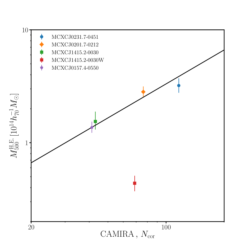
Figure 8: A comparison between CAMIRA richness (Oguri et al. 2017) and HE mass at $\Delta=500$. A solid line is the best-fit for the four MCXC clusters. The H.E. mass for the non-MCXC cluster is significantly lower than the best-fit base line.

6.6 Mass comparison

We compare WL masses with H.E. masses at $\Delta=500$, as a first attempt of our further studies. The full-depth and full-colour conditions allows us to compare the two masses only for the three clusters. The X-ray and WL mass measurements are described in Sections 3.5 and 5, respectively. As in previous studies of hydrostatic mass bias (Mahdavi et al. 2013; von der Linden et al. 2014; Okabe et al. 2014b; Hoekstra et al. 2015; Smith et al. 2016), a comparison of H.E. and WL mass gives an indirect constraint on the degree to which the assumption that clusters are in H.E. is valid for cosmological applications. We deliberately perform a simpler calculation of mass bias because of the observational limitation of the current sample. The mass comparison adopts the masses enclosed within the overdensity radii independently determined by different measurements. When we compare the masses measured within the same apertures, the results do not change and thus the aperture mismatching is a subdominant effect. We adopt the unweighted geometric mean to quantify the mass bias $b_{m}$,

$$b_{m}=1-\prod_{i}^{n}\left(\frac{M_{\rm H.E.}}{M_{\rm WL}}\right)_{i}^{1/n}.$$ (23)

When we exchange $M_{\rm H.E.}$ for $M_{\rm WL}$ in the equation, the second term of this quantity becomes the inverse in contrast to an estimation with $\sum_{i}\left(M_{\rm H.E.}/M_{\rm WL}\right)_{i}/n$. If the H.E. mass is statistically consistent with the WL mass, the bias parameter, $b_{m}$ is equal to zero. We obtain $b_{m}=0.44_{-0.45}^{+0.31}$, for the three clusters at $\Delta=500$ (Figure 9). We also obtain $b_{m}=0.34_{-0.19}^{+0.16}$ for the two MCXC clusters. Since the measurement errors for WL masses of the two MCXC clusters are relatively small, the error of $b_{m}$ becomes smaller. It indicates that the H.E. mass at $\Delta=500$ is consistent with the WL mass in the current sample at the $2\sigma$ level.

When we use the same radii determined by weak-lensing masses, we obtain $b_{m}=0.40_{-0.49}^{+0.39}$ for the three clusters and $b_{m}=0.34_{-0.41}^{+0.28}$ for the two clusters, respectively. We here consider the error propagation of measurement uncertainties of the WL radii. The result does not significantly change. When we measure WL masses with X-ray centers, the best-fit WL masses are changed only by a few percent because the offset distances between X-ray centroids and BCG positions are very small.

Although our results are statistically poor because of a small sample of clusters, we compare with the literature. Direct comparisons between weak-lensing masses and X-ray masses are not trivial, because previous studies applied their own methods: the boost factor correction (e.g. von der Linden et al. 2014; Hoekstra et al. 2015) or no correction (e.g. Okabe et al. 2016; Umetsu et al. 2016) in WL analyses and emission-weighted temperatures (e.g. Zhang et al. 2008; Mahdavi et al. 2013) or spectroscopic-like temperature (e.g. Mazzotta et al. 2004; Martino et al. 2014) in X-ray analyses. Smith et al. (2016) obtained the average bias $b_{m}=0.05\pm 0.05$ for fifty clusters at $z\sim 0.2$, and Mahdavi et al. (2013) computed $b_{m}=0.12\pm 0.05$ with their WL radii. Using the same sample between the two papers, the major difference ($\sim 10\%$) would come from X-ray mass measurements (Smith et al. 2016). We here assume that the difference is mainly caused by temperature definitions and discuss this possibility. Mazzotta et al. (2004) discovered using realistic simulations that the H.E. mass estimations with emission-weighted temperatures would be underestimated by $\sim 10\%$ and those with spectroscopic-like temperature would recover the input mass. When we estimate the H.E masses with emission-weighted temperatures, the masses are indeed lower $\sim 10\%$ than our results. Therefore, the possibility does not conflict with a difference between the two papers (Mahdavi et al. 2013; Smith et al. 2016). However, the current uncertainty for the averaged bias is too large to discuss the details. When we compile the full sample of $22$ clusters, we expect that the uncertainty for the average bias will be comparable to those for previous studies for $50$ clusters (Hoekstra et al. 2015; Smith et al. 2016). We therefore will compare WL and H.E. masses for the full sample, and investigate the redshift dependence and radial dependence of the mass bias.

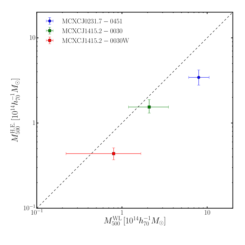
Figure 9: Mass comparison of WL and H.E. masses for the three clusters at $\Delta=500$.

6.7 Baryon Fraction

The ratio of baryonic-to-total mass in massive clusters is expected to closely match the cosmic mean baryon fraction, $\Omega_{b}/\Omega_{m}$ measured from CMB experiments if baryons are trapped in potential wells (e.g. Evrard 1997; Kravtsov et al. 2005). However, the baryon budget in galaxy clusters is sensitive to non-gravitational process; stars are formed from gas through radiative cooling and AGN feedback may push the gas outside the potential well. Thus, measurements of the cluster baryon fraction are important to understand baryonic physics and the interplay between baryons and dark matter. Furthermore, assuming that the gas mass fraction is constant across redshifts, gas mass fraction measurements potentially provide a cosmological probe (e.g. Allen et al. 2008).

This paper focuses on the baryon fraction at $\Delta=500$ based on the H.E. mass, because the result based on the WL mass is statistically poor. We define gas and baryon fraction as follows:

$$f_{\rm gas}(<r) = \frac{M_{\rm gas}(<r)}{M_{\rm H.E.}(<r)},$$

$$f_{\rm b}(<r) = \frac{M_{\rm gas}(<r)+M_{\rm*}(<r)}{M_{\rm H.E.}(<r)}.$$

Here, $M_{\rm gas}$, $M_{*}$ and $M_{\rm H.E.}$ are gas, stellar and H.E. masses (Table 3), respectively. Gas mass is measured from X-ray analysis. Stellar masses are delivered from the deprojection estimation of the CAMIRA cluster catalog using the HSC-SSP five-band photometry (Section 4). Measurement uncertainty of the total mass propagates through the over-density radius into gas and stellar masses. Figure 10 shows the gas and baryon fractions based on H.E. masses.

We also investigated how much the stellar mass estimation is changed if blue galaxies are included. We selected blue galaxies of which colors are bluer by $1-3\sigma$ than those of the red-sequence galaxies within $r_{500}$ and estimated their stellar mass in a cylinder volume subtracted by $(2-3)r_{500}$ as the background region. The total stellar masses are changed only by sub-$\%$. Even if we neither subtract the background components nor change the background region, the result does not significantly change. It is not surprising because the faint and blue galaxies are not dominant contributors to the light or stellar mass in cluster central regions, in contrast to the bright and red galaxies. We note that the stellar mass estimation for blue galaxies is within the projected cylinder volume because the characteristic spatial distribution for the blue galaxies (essentially a hollowed-out sphere) makes it impractical to carry out the deprojection method. We stress that we estimated the total stellar mass using red galaxies in a spherical volume using the deprojection method (Section 4).

In contrast to previous observational studies (e.g. Lin et al. 2003; Vikhlinin et al. 2009b) showing that gas mass fraction increases and stellar mass fraction decreases with a total mass increasing, we find no significant evidence of a halo mass dependence of $f_{\rm gas}$ and $f_{*}$ in the current sample. The relation might be difficult to measure given the intrinsic scatter and the small sample size. We therefore focus on a comparison between the averages for $f_{\rm gas}$ and $f_{*}$ for the current sample and the literature. Based on the defined selection function of the MCXC clusters, we compute unweighted averages of gas and baryon fractions for the four MCXC clusters.

To investigate a mass dependence of $f_{\rm gas}$ using the literature, we plot the averaged fraction enclosed within $r_{500}$ and mass plane (left panel of Figure 11). The average value is $\langle f_{\rm gas}\rangle=0.125\pm 0.012$, which is in agreement with previous studies based on H.E. mass or Sunyaev-Zel’dovich effect (SZE) mass (e.g. Vikhlinin et al. 2009a; Martino et al. 2014; Sun et al. 2009; Chiu et al. 2016) and based on WL masses (e.g. Zhang et al. 2010; Mahdavi et al. 2013; Okabe et al. 2014b). All points are unweighted averages from tables in the literature. Differences for those gas fractions at $M_{500}\sim 2.4\times 10^{14}\mathrel{h_{70}^{-1}M_{\odot}}$ and $\sim 7\times 10^{14}\mathrel{h_{70}^{-1}M_{\odot}}$ are $\sim 8\%$ and $\sim 6\%$, respectively. However, the gas fraction of the XXL survey (Eckert et al. 2016) is systematically lower than in other studies in a wide mass range. The deviation is at the $\sim 5.3\sigma$ level, where we use the $8\%$ scatter. In our sample of the four MCXC clusters, the gas mass fraction is $\sim 0.8\pm 0.1$ of the cosmic mean baryon fraction $\Omega_{b}/\Omega_{m}$ for WMAP (Hinshaw et al. 2013) and $\sim 0.9\pm 0.1$ for Planck (Planck Collaboration 2015), though the two experiments have reported slightly discrepant results. The values are slightly higher than $f_{\rm gas}\Omega_{m}/\Omega_{b}\sim 0.6$ from numerical simulations (e.g. Kravtsov et al. 2005; Planelles et al. 2013; Battaglia et al. 2013).

The average baryon fraction for the four MCXC clusters, $\langle f_{\rm b}\rangle=0.146\pm 0.012$, is comparable to $\Omega_{b}/\Omega_{m}$ (right panel of Figure 11). Our result is also comparable to previous observational studies (Lin et al. 2003, 2012; Giodini et al. 2009; Laganá et al. 2011; Chiu et al. 2016). A difference between those baryon fractions at $M_{500}\sim 2.4\times 10^{14}\mathrel{h_{70}^{-1}M_{\odot}}$ is only $\sim 7\%$. There are some discrepancies in $f_{b}$ even between different numerical simulations. Kravtsov et al. (2005) have shown that the total baryon fraction agrees with $\Omega_{b}/\Omega_{m}$, while Planelles et al. (2013) have pointed out that it accounts for $\sim 85\%$ because some fraction of gas is displaced outside potential wells by AGN activities.

We also note that, if there were H.E. mass bias, the gas and baryon fractions would be overestimated. Observations of baryon budget in galaxy clusters are still open questions. Since small clusters and groups are sensitive to baryonic physics (e.g. Kravtsov et al. 2005; Planelles et al. 2013; Battaglia et al. 2013), future progress of the HSC-SSP survey and future studies based on WL masses will play a key role in this subject.

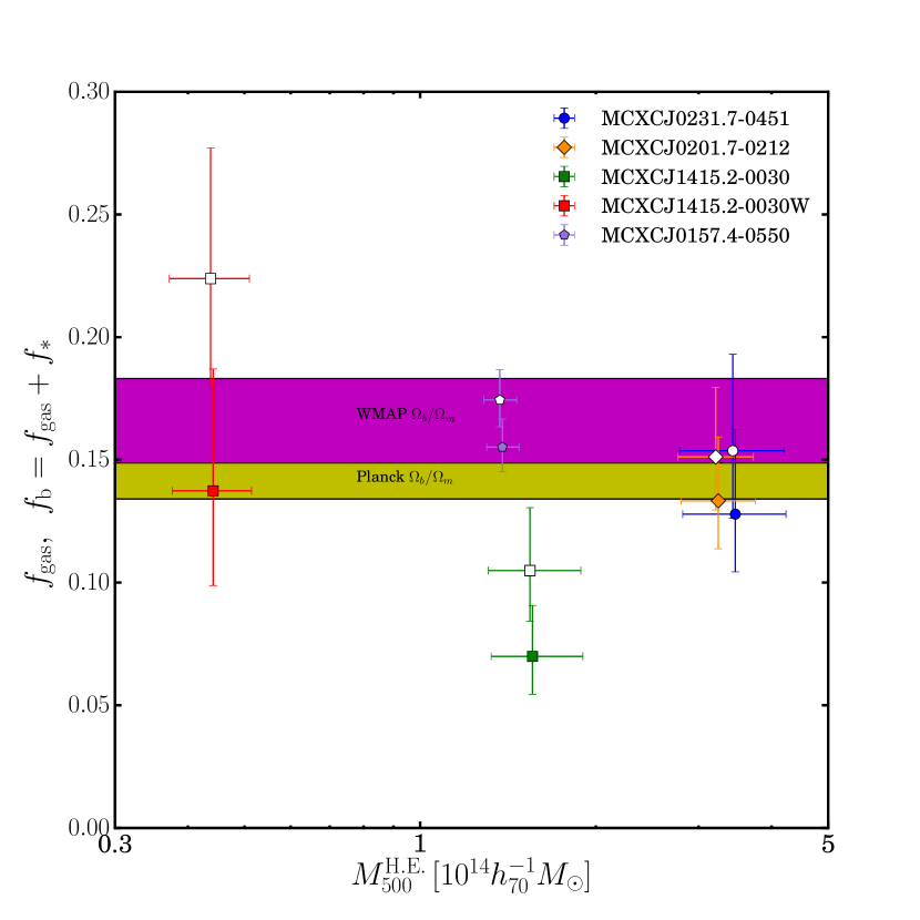
Figure 10: Gas fraction (filled symbols), $f_{\rm gas}$, and baryon fraction (opened symbols), $f_{\rm b}$, within $r_{500}$ based on H.E. masses. The horizontal filled regions are the cosmic mean baryon fraction $\Omega_{b}/\Omega_{m}$ for WMAP (Hinshaw et al. 2013) and Planck (Planck Collaboration 2015) with their respective $1\sigma$ uncertainties. For a visual purpose, the H.E. masses of the gas fractions are multiplied by $1.01$.

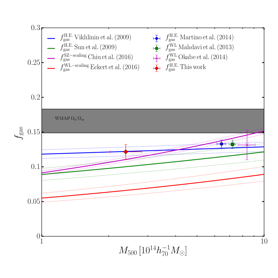
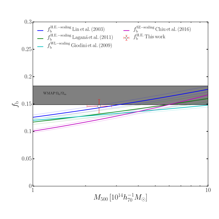
Figure 11: Comparison with the literature : gas fraction (left) and baryon fraction (right). Left : Red diamond is the average for $f_{\rm gas}$ for the four MCXC clusters. Blue circle, green square and magenta cross are $\langle f_{\rm gas}\rangle$ from Martino et al. (2014), Mahdavi et al. (2013) and Okabe et al. (2014b), respectively. Blue, green, magenta and red solid lines are scaling functions between gas fraction and mass from Vikhlinin et al. (2009a), Sun et al. (2009), Chiu et al. (2016), and Eckert et al. (2016), respectively. Dotted lines are $1\sigma$ uncertainties of the scaling functions. For simplicity, we plot $\Omega_{b}/\Omega_{m}$ for WMAP (Hinshaw et al. 2013). Upper superscripts denote methods of total mass estimation. Right : White diamond are the average for $f_{\rm b}$ for the four MCXC clusters, derived by this study. Blue, green, cyan and magenta solid lines are scaling functions between baryon fraction and mass from Lin et al. (2003), Laganá et al. (2011), Giodini et al. (2009), and Chiu et al. (2016). respectively.

7 Summary

We selected X-ray luminous clusters from the MCXC cluster catalog (Piffaretti et al. 2011) to measure H.E. masses for galaxy clusters in the HSC-SSP survey region. Based on the XMM-Newton and HSC-SSP datasets, we carried out a multiwavelength study of four MCXC clusters in the S16A field and a non-MCXC cluster associated with one MCXC cluster.

We found a correlation between cluster richness and H.E. mass for the MCXC clusters. The mass normalization agrees with expectations by comparing the CAMIRA cluster abundance with a theoretical prediction of cluster mass function with $\sigma_{8}=0.82$ (Oguri et al. 2017). However, an infalling cluster to one MCXC cluster is highly deviant from the scaling relation, which could be caused by mass underestimation and/or richness overestimation. The average cluster gas mass fraction based on H.E. masses, $\langle f_{\rm b}\rangle=0.146\pm 0.012$, accounts for $\sim 80-90\%$ of the cosmic mean baryon fraction. In comparison with gas and baryon fractions from the literature based on various mass measurements (Vikhlinin et al. 2009a; Martino et al. 2014; Mahdavi et al. 2013; Okabe et al. 2014b; Sun et al. 2009; Eckert et al. 2016; Giodini et al. 2009; Chiu et al. 2016), our measurements are somewhat higher than previous studies but overall are agreed. Differences of gas and baryon fractions between these studies are $\sim 8\%$ and $\sim 7\%$ at $M_{500}\sim 2.4\times 10^{14}\mathrel{h_{70}^{-1}M_{\odot}}$, respectively. We also note a possibility that the average gas and baryon fraction is somehow overestimated if there were H.E. mass bias. Therefore, future studies using WL masses for a large number of clusters/groups will be important to understand the baryon budgets and improve the current level of the quality.

The full-depth and full-colour conditions of the HSC-SSP survey allows us to compare H.E. mass with WL mass for the three clusters. The estimated mass bias, $b_{m}=0.44^{+0.31}_{-0.45}$, allows for the possibility that the H.E. masses agree with the WL ones. In order to quantify the validly of H.E. assumption, we need to carry out WL analysis for the full sample of clusters.

Further joint studies using a large number of clusters are vitally important to improve statistical uncertainty. Pointed X-ray observations with XMM-Newton and Chandra with sufficient integration times are essential to fairly compare X-ray observables with WL and optical measurements. The approach is complementary to the forthcoming X-ray survey from eROSITA, whose typical exposure in the HSC-SSP survey region is too shallow to estimate H.E. masses. A collaboration with the on-going XXL survey is powerful to understand cluster physics and carry out cluster-based cosmology. In similar ways, joint studies with the ACTPol SZE observations (Miyatake et al. in prep) provide us with an unique route for cluster studies. Future studies based on survey-type datasets will also reveal how much cluster properties are changed by cluster selection methods, like X-ray, SZE, optical and WL techniques. The paper has demonstrated the power and impact of the HSC-SSP survey on other wavelengths and shown the first result as a series of multiwavelength studies.

The Hyper Suprime-Cam (HSC) collaboration includes the astronomical communities of Japan and Taiwan, and Princeton University. The HSC instrumentation and software were developed by the National Astronomical Observatory of Japan (NAOJ), the Kavli Institute for the Physics and Mathematics of the Universe (Kavli IPMU), the University of Tokyo, the High Energy Accelerator Research Organization (KEK), the Academia Sinica Institute for Astronomy and Astrophysics in Taiwan (ASIAA), and Princeton University. Funding was contributed by the FIRST program from Japanese Cabinet Office, the Ministry of Education, Culture, Sports, Science and Technology (MEXT), the Japan Society for the Promotion of Science (JSPS), Japan Science and Technology Agency (JST), the Toray Science Foundation, NAOJ, Kavli IPMU, KEK, ASIAA, and Princeton University.

This paper makes use of software developed for the Large Synoptic Survey Telescope. We thank the LSST Project for making their code available as free software at http://dm.lsst.org

The Pan-STARRS1 Surveys (PS1) have been made possible through contributions of the Institute for Astronomy, the University of Hawaii, the Pan-STARRS Project Office, the Max-Planck Society and its participating institutes, the Max Planck Institute for Astronomy, Heidelberg and the Max Planck Institute for Extraterrestrial Physics, Garching, The Johns Hopkins University, Durham University, the University of Edinburgh, Queen’s University Belfast, the Harvard-Smithsonian Center for Astrophysics, the Las Cumbres Observatory Global Telescope Network Incorporated, the National Central University of Taiwan, the Space Telescope Science Institute, the National Aeronautics and Space Administration under Grant No. NNX08AR22G issued through the Planetary Science Division of the NASA Science Mission Directorate, the National Science Foundation under Grant No. AST-1238877, the University of Maryland, and Eotvos Lorand University (ELTE) and the Los Alamos National Laboratory.

Based on data collected at the Subaru Telescope and retrieved from the HSC data archive system, which is operated by Subaru Telescope and Astronomy Data Center at National Astronomical Observatory of Japan.

This work was supported by the Funds for the Development of Human Resources in Science and Technology under MEXT, Japan and Core Research for Energetic Universe in Hiroshima University (the MEXT program for promoting the enhancement of research universities, Japan). This work was supported in part by World Premier International Research Center Initiative (WPI Initiative), MEXT, Japan. This work was supported by MEXT KAKENHI No. 26800097(NO), 26800093/15H05892(MO), 15K05080 (YF), 26400218 (MT) and 15K17610 (SU). HM is supported by the Jet Propulsion Laboratory, California Institute of Technology, under a contract with the National Aeronautics and Space Administration.

The paper is dedicated to the memory of our friend, Dr. Yuying Zhang, who sadly passed away in 2016. She gave helpful suggestions on our X-ray analysis.

Appendix A Results of Spectral fit

We summarize results of simultaneous fit for the spectrum in Table 4. The technical details are described in Sec. 3.

Table 4: Cluster details. ^aCluster name. ^bCluster-centric annulus ^c counts in the energy band of 0.3-11 KeV of each instrument. ^d Best-fit temperature and ^e Best-fit abundance

Namea	Annulusb	counts$\pm$errorc			Temperatured	Abandancee
	(arcsec)	MOS1	MOS2	PN	(keV)	($Z_{\odot}$)
MCXCJ0157.4-0550	0- 60	834	829	1400	$3.51_{-0.26}^{+0.32}$	$0.26$
	60-100	1038	1163	1975	$3.02_{-0.22}^{+0.27}$	$0.18$
	100-140	1196	1267	1955	$3.28_{-0.25}^{+0.33}$	$0.18$
	140-180	1228	1303	2085	$2.84_{-0.23}^{+0.30}$	$0.20$
	180-270	2867	2732	4647	$2.73_{-0.13}^{+0.28}$	$0.16$
	270-360	2920	2640	5306	$2.54_{-0.10}^{+0.31}$	$0.10$
	360-600	7778	8959	17871	-
	600-900	3117	5036	13795	-
MCXCJ0231.7-0451	0- 40	1411	1355	3084	$5.64_{-0.34}^{+0.40}$	$0.52$
	40- 60	1381	1353	2739	$5.03_{-0.37}^{+0.37}$	$0.12$
	60- 80	1339	1229	2492	$4.33_{-0.27}^{+0.36}$	$0.46$
	80-100	1182	1198	2455	$5.03_{-0.47}^{+0.52}$	$0.33$
	100-140	1936	1882	3737	$4.09_{-0.22}^{+0.23}$	$0.20$
	140-180	1155	1174	2052	$4.50_{-0.44}^{+0.55}$	$0.20$
	180-270	1665	1591	3373	$3.10_{-0.38}^{+0.54}$	$0.20$
	270-400	1633	1798	4002	-
MCXCJ0201.7-0212	0- 40	7690	7369	16494	$3.30_{-0.05}^{+0.05}$	$0.41$
	40- 60	2617	2379	4139	$4.23_{-0.27}^{+0.36}$	$0.28$
	60- 80	1649	1686	3218	$4.26_{-0.36}^{+0.48}$	$0.14$
	80-100	1157	1151	2440	$4.47_{-0.69}^{+0.58}$	$0.14$
	100-140	1667	1710	3198	$3.38_{-0.20}^{+0.41}$	$0.17$
	140-180	1044	1034	1750	$4.28_{-0.49}^{+0.67}$	$0.17$
	180-270	1596	1719	2486	$2.43_{-0.28}^{+0.27}$	$0.17$
	270-360	1324	1502	2463	-
MCXCJ1415.2-0030	0- 50	509	519	889	$3.12_{-0.25}^{+0.25}$	$0.22$
	50- 90	690	683	1102	$3.99_{-0.41}^{+0.46}$	$0.29$
	90-140	761	736	1522	$3.00_{-0.34}^{+0.31}$	$0.47$
	140-180	481	444	890	$2.03_{-0.38}^{+0.54}$	$0.21$
	180-270	969	953	1984	$1.71_{-0.13}^{+0.12}$	$0.12$
	270-360	1302	1225	2653	-	-
MCXCJ1415.2-0030W	0-80	191	229	417	$2.06_{-0.22}^{+0.29}$	$0.34$
	80-140	198	246	430	$1.80_{-0.28}^{+0.94}$	$0.33$
	140-270	772	803	1473	-

References

- Aihara et al. (2017a) Aihara, H., Armstrong, R., Bickerton, S., et al. 2017a, ArXiv e-prints
- Aihara et al. (2017b) Aihara, H., Arimoto, N., Armstrong, R., et al. 2017b, ArXiv e-prints
- Allen et al. (2008) Allen, S. W., Rapetti, D. A., Schmidt, R. W., et al. 2008, MNRAS, 383, 879
- Anders & Grevesse (1989) Anders, E., & Grevesse, N. 1989, Geochim. Cosmochim. Acta, 53, 197
- Austermann et al. (2012) Austermann, J. E., Aird, K. A., Beall, J. A., et al. 2012, in Proc. SPIE, Vol. 8452, Millimeter, Submillimeter, and Far-Infrared Detectors and Instrumentation for Astronomy VI, 84521E
- Avestruz et al. (2016) Avestruz, C., Nagai, D., & Lau, E. T. 2016, ArXiv e-prints
- Balucinska-Church & McCammon (1992) Balucinska-Church, M., & McCammon, D. 1992, ApJ, 400, 699
- Bartelmann & Schneider (2001) Bartelmann, M., & Schneider, P. 2001, Phys. Rep., 340, 291
- Battaglia et al. (2013) Battaglia, N., Bond, J. R., Pfrommer, C., & Sievers, J. L. 2013, ApJ, 777, 123
- Becker & Kravtsov (2011) Becker, M. R., & Kravtsov, A. V. 2011, ApJ, 740, 25
- Bleem et al. (2015) Bleem, L. E., Stalder, B., de Haan, T., et al. 2015, ApJS, 216, 27
- Broadhurst et al. (2005) Broadhurst, T., Takada, M., Umetsu, K., et al. 2005, ApJ, 619, L143
- Cappelluti et al. (2011) Cappelluti, N., Predehl, P., Böhringer, H., et al. 2011, Memorie della Societa Astronomica Italiana Supplementi, 17, 159
- Carrasco Kind & Brunner (2014) Carrasco Kind, M., & Brunner, R. J. 2014, MNRAS, 438, 3409
- Cavaliere & Fusco-Femiano (1976) Cavaliere, A., & Fusco-Femiano, R. 1976, A&A, 49, 137
- Chiu et al. (2016) Chiu, I., Mohr, J., McDonald, M., et al. 2016, MNRAS, 455, 258
- Dark Energy Survey Collaboration et al. (2016) Dark Energy Survey Collaboration, Abbott, T., Abdalla, F. B., et al. 2016, MNRAS, 460, 1270
- Diemer & Kravtsov (2014) Diemer, B., & Kravtsov, A. V. 2014, ArXiv e-prints
- Donahue et al. (2014) Donahue, M., Voit, G. M., Mahdavi, A., et al. 2014, ApJ, 794, 136
- Eckert et al. (2016) Eckert, D., Ettori, S., Coupon, J., et al. 2016, A&A, 592, A12
- Evrard (1997) Evrard, A. E. 1997, MNRAS, 292, 289
- Fujita et al. (2013) Fujita, Y., Ohira, Y., & Yamazaki, R. 2013, ApJ, 767, L4
- Giodini et al. (2009) Giodini, S., Pierini, D., Finoguenov, A., et al. 2009, ApJ, 703, 982
- Hasselfield et al. (2013) Hasselfield, M., Hilton, M., Marriage, T. A., et al. 2013, J. Cosmology Astropart. Phys, 7, 008
- Heymans et al. (2006) Heymans, C., Van Waerbeke, L., Bacon, D., et al. 2006, MNRAS, 368, 1323
- Hinshaw et al. (2013) Hinshaw, G., Larson, D., Komatsu, E., et al. 2013, ApJS, 208, 19
- Hirata & Seljak (2003) Hirata, C., & Seljak, U. 2003, MNRAS, 343, 459
- Hoekstra (2003) Hoekstra, H. 2003, MNRAS, 339, 1155
- Hoekstra et al. (2015) Hoekstra, H., Herbonnet, R., Muzzin, A., et al. 2015, The Canadian Cluster Comparison Project: detailed study of systematics and updated weak lensing masses
- Ilbert et al. (2013) Ilbert, O., McCracken, H. J., Le Fèvre, O., et al. 2013, A&A, 556, A55
- Jones & Forman (1984) Jones, C., & Forman, W. 1984, ApJ, 276, 38
- Kalberla et al. (2005) Kalberla, P. M. W., Burton, W. B., Hartmann, D., et al. 2005, A&A, 440, 775
- Kawaharada et al. (2010) Kawaharada, M., Okabe, N., Umetsu, K., et al. 2010, ApJ, 714, 423
- Kravtsov et al. (2005) Kravtsov, A. V., Nagai, D., & Vikhlinin, A. A. 2005, ApJ, 625, 588
- Laganá et al. (2011) Laganá, T. F., Zhang, Y.-Y., Reiprich, T. H., & Schneider, P. 2011, ApJ, 743, 13
- Lapi et al. (2010) Lapi, A., Fusco-Femiano, R., & Cavaliere, A. 2010, A&A, 516, A34
- Lieu et al. (2016) Lieu, M., Smith, G. P., Giles, P. A., et al. 2016, A&A, 592, A4
- Lin et al. (2003) Lin, Y.-T., Mohr, J. J., & Stanford, S. A. 2003, ApJ, 591, 749
- Lin et al. (2004) —. 2004, ApJ, 610, 745
- Lin et al. (2012) Lin, Y.-T., Stanford, S. A., Eisenhardt, P. R. M., et al. 2012, ApJ, 745, L3
- Louis et al. (2016) Louis, T., Grace, E., Hasselfield, M., et al. 2016, ArXiv e-prints
- Mahdavi et al. (2013) Mahdavi, A., Hoekstra, H., Babul, A., et al. 2013, ApJ, 767, 116
- Mandelbaum et al. (2006) Mandelbaum, R., Seljak, U., Kauffmann, G., Hirata, C. M., & Brinkmann, J. 2006, MNRAS, 368, 715
- Mandelbaum et al. (2005) Mandelbaum, R., Hirata, C. M., Seljak, U., et al. 2005, MNRAS, 361, 1287
- Mandelbaum et al. (2014) Mandelbaum, R., Rowe, B., Bosch, J., et al. 2014, ApJS, 212, 5
- Mandelbaum et al. (2015) Mandelbaum, R., Rowe, B., Armstrong, R., et al. 2015, MNRAS, 450, 2963
- Mandelbaum et al. (2017a) Mandelbaum, R., Miyatake, H., Hamana, T., et al. 2017a, ArXiv:1705.06745
- Mandelbaum et al. (2017b) Mandelbaum, R., Lanusse, F., Leauthaud, A., et al. 2017b, ArXiv e-prints
- Mantz et al. (2016) Mantz, A. B., Allen, S. W., Morris, R. G., & Schmidt, R. W. 2016, MNRAS, 456, 4020
- Martino et al. (2014) Martino, R., Mazzotta, P., Bourdin, H., et al. 2014, MNRAS, 443, 2342
- Massey et al. (2007) Massey, R., Heymans, C., Bergé, J., et al. 2007, MNRAS, 376, 13
- Mazzotta et al. (2004) Mazzotta, P., Rasia, E., Moscardini, L., & Tormen, G. 2004, MNRAS, 354, 10
- Medezinski et al. (2010) Medezinski, E., Broadhurst, T., Umetsu, K., et al. 2010, MNRAS, 405, 257
- Medezinski et al. (2015) Medezinski, E., Umetsu, K., Okabe, N., et al. 2015, ArXiv e-prints
- Medezinski et al. (2017) Medezinski, E., Oguri, M., Nishizawa, A. J., et al. 2017, ArXiv 1706.00427
- Melchior et al. (2016) Melchior, P., Gruen, D., McClintock, T., et al. 2016, ArXiv e-prints
- Meneghetti et al. (2010) Meneghetti, M., Rasia, E., Merten, J., et al. 2010, A&A, 514, A93
- Miyatake et al. (2013) Miyatake, H., Nishizawa, A. J., Takada, M., et al. 2013, MNRAS, 429, 3627
- Miyatake et al. (in prep) Miyatake et al. in prep, PASJ
- Miyazaki et al. (2012) Miyazaki, S., Komiyama, Y., Nakaya, H., et al. 2012, in Proc. SPIE, Vol. 8446, Ground-based and Airborne Instrumentation for Astronomy IV, 84460Z
- Miyazaki et al. (2015) Miyazaki, S., Oguri, M., Hamana, T., et al. 2015, ApJ, 807, 22
- Navarro et al. (1996) Navarro, J. F., Frenk, C. S., & White, S. D. M. 1996, ApJ, 462, 563
- Navarro et al. (1997) —. 1997, ApJ, 490, 493
- Oguri (2014) Oguri, M. 2014, MNRAS, 444, 147
- Oguri et al. (2012) Oguri, M., Bayliss, M. B., Dahle, H., et al. 2012, MNRAS, 420, 3213
- Oguri et al. (2010) Oguri, M., Takada, M., Okabe, N., & Smith, G. P. 2010, MNRAS, 405, 2215
- Oguri et al. (2005) Oguri, M., Takada, M., Umetsu, K., & Broadhurst, T. 2005, ApJ, 632, 841
- Oguri et al. (2017) Oguri, M., Lin, Y.-T., Lin, S.-C., et al. 2017, ArXiv e-prints
- Okabe et al. (2014a) Okabe, N., Futamase, T., Kajisawa, M., & Kuroshima, R. 2014a, ApJ, 784, 90
- Okabe & Smith (2016) Okabe, N., & Smith, G. P. 2016, MNRAS, 461, 3794
- Okabe et al. (2013) Okabe, N., Smith, G. P., Umetsu, K., Takada, M., & Futamase, T. 2013, ApJ, 769, L35
- Okabe et al. (2010) Okabe, N., Takada, M., Umetsu, K., Futamase, T., & Smith, G. P. 2010, PASJ, 62, 811
- Okabe & Umetsu (2008) Okabe, N., & Umetsu, K. 2008, PASJ, 60, 345
- Okabe et al. (2014b) Okabe, N., Umetsu, K., Tamura, T., et al. 2014b, PASJ, 66, 99
- Okabe et al. (2016) —. 2016, MNRAS, 456, 4475
- Owers et al. (2013) Owers, M. S., Baldry, I. K., Bauer, A. E., et al. 2013, ApJ, 772, 104
- Pierre et al. (2016) Pierre, M., Pacaud, F., Adami, C., et al. 2016, A&A, 592, A1
- Piffaretti et al. (2011) Piffaretti, R., Arnaud, M., Pratt, G. W., Pointecouteau, E., & Melin, J.-B. 2011, A&A, 534, A109
- Planck Collaboration (2015) Planck Collaboration. 2015, ArXiv e-prints
- Planck Collaboration et al. (2015) Planck Collaboration, Ade, P. A. R., Aghanim, N., et al. 2015, ArXiv e-prints
- Planelles et al. (2013) Planelles, S., Borgani, S., Dolag, K., et al. 2013, MNRAS, 431, 1487
- Pratt et al. (2010) Pratt, G. W., Arnaud, M., Piffaretti, R., et al. 2010, A&A, 511, A85
- Reyes et al. (2012) Reyes, R., Mandelbaum, R., Gunn, J. E., et al. 2012, MNRAS, 425, 2610
- Schneider et al. (1998) Schneider, P., van Waerbeke, L., Jain, B., & Kruse, G. 1998, MNRAS, 296, 873
- Shan et al. (2012) Shan, H., Kneib, J.-P., Tao, C., et al. 2012, ApJ, 748, 56
- Simet et al. (2017) Simet, M., McClintock, T., Mandelbaum, R., et al. 2017, MNRAS, 466, 3103
- Smith et al. (2016) Smith, G. P., Mazzotta, P., Okabe, N., et al. 2016, MNRAS, 456, L74
- Smith et al. (2001) Smith, R. K., Brickhouse, N. S., Liedahl, D. A., & Raymond, J. C. 2001, ApJ, 556, L91
- Snowden et al. (2008) Snowden, S. L., Mushotzky, R. F., Kuntz, K. D., & Davis, D. S. 2008, A&A, 478, 615
- Snowden et al. (1997) Snowden, S. L., Egger, R., Freyberg, M. J., et al. 1997, ApJ, 485, 125
- Strüder et al. (2001) Strüder, L., Briel, U., Dennerl, K., et al. 2001, A&A, 365, L18
- Sun et al. (2009) Sun, M., Voit, G. M., Donahue, M., et al. 2009, ApJ, 693, 1142
- Tanaka et al. (2017) Tanaka, M., Coupon, J., Hsieh, B.-C., et al. 2017, ArXiv e-prints
- Tinker et al. (2010) Tinker, J. L., Robertson, B. E., Kravtsov, A. V., et al. 2010, ApJ, 724, 878
- Turner et al. (2001) Turner, M. J. L., Abbey, A., Arnaud, M., et al. 2001, A&A, 365, L27
- Umetsu et al. (2011) Umetsu, K., Broadhurst, T., Zitrin, A., et al. 2011, ApJ, 738, 41
- Umetsu et al. (2016) Umetsu, K., Zitrin, A., Gruen, D., et al. 2016, ApJ, 821, 116
- Vikhlinin et al. (2006) Vikhlinin, A., Kravtsov, A., Forman, W., et al. 2006, ApJ, 640, 691
- Vikhlinin et al. (2009a) Vikhlinin, A., Burenin, R. A., Ebeling, H., et al. 2009a, ApJ, 692, 1033
- Vikhlinin et al. (2009b) Vikhlinin, A., Kravtsov, A. V., Burenin, R. A., et al. 2009b, ApJ, 692, 1060
- von der Linden et al. (2014) von der Linden, A., Mantz, A., Allen, S. W., et al. 2014, MNRAS, 443, 1973
- Walker et al. (2012) Walker, S. A., Fabian, A. C., Sanders, J. S., & George, M. R. 2012, MNRAS, 427, L45
- Yang et al. (2006) Yang, X., Mo, H. J., van den Bosch, F. C., et al. 2006, MNRAS, 373, 1159
- Zhang et al. (2008) Zhang, Y.-Y., Finoguenov, A., Böhringer, H., et al. 2008, A&A, 482, 451
- Zhang et al. (2010) Zhang, Y.-Y., Okabe, N., Finoguenov, A., et al. 2010, ApJ, 711, 1033