The first-year shear catalog of the Subaru Hyper Suprime-Cam SSP Survey

Abstract

We present and characterize the catalog of galaxy shape measurements that will be used for cosmological weak lensing measurements in the Wide layer of the first year of the Hyper Suprime-Cam (HSC) survey. The catalog covers an area of 136.9 deg² split into six fields, with a mean $i$-band seeing of $0.58$ and $5\sigma$ point-source depth of $i\sim 26$. Given conservative galaxy selection criteria for first year science, the depth and excellent image quality results in unweighted and weighted source number densities of 24.6 and 21.8 arcmin^-2, respectively. We define the requirements for cosmological weak lensing science with this catalog, then focus on characterizing potential systematics in the catalog using a series of internal null tests for problems with point-spread function (PSF) modeling, shear estimation, and other aspects of the image processing. We find that the PSF models narrowly meet requirements for weak lensing science with this catalog, with fractional PSF model size residuals of approximately $0.003$ (requirement: 0.004) and the PSF model shape correlation function $\rho_{1}<3\times 10^{-7}$ (requirement: $4\times 10^{-7}$) at 0.5^∘ scales. A variety of galaxy shape-related null tests are statistically consistent with zero, but star-galaxy shape correlations reveal additive systematics on on $>1^{\circ}$ scales that are sufficiently large as to require mitigation in cosmic shear measurements. Finally, we discuss the dominant systematics and the planned algorithmic changes to reduce them in future data reductions.

1 Introduction

The currently accepted cosmological model that is broadly consistent with multiple observations, $\Lambda$CDM, is dominated by dark ingredients: dark matter, which we observe through its gravitational effects, and dark energy, the presence of which was inferred due to the accelerated expansion of the universe as detected using supernovae (Riess et al., 1998; Perlmutter et al., 1999). Weak gravitational lensing provides us with a way of observing the total matter density (including dark matter), via the deflections of light due to intervening matter along the line-of-sight, which both magnifies and distorts galaxy shapes (for recent reviews, see Weinberg et al., 2013; Kilbinger, 2015). The lensing measurement that is commonly used to constrain the amplitude and growth of matter fluctuations is ‘cosmic shear’, the auto-correlation of galaxy shape distortions. When measured in redshift bins (‘tomography’), cosmic shear is particularly powerful at tracing structure growth as a function of time. Since the initial detections of cosmic shear a decade ago (Bacon et al., 2000; Van Waerbeke et al., 2000; Rhodes et al., 2001; Hoekstra et al., 2002), ever larger datasets and increasingly sophisticated measurement techniques have led to steadily decreasing errors, both statistical and systematic (e.g., most recently, Heymans et al., 2013; Becker et al., 2016; Jee et al., 2016; Hildebrandt et al., 2017).

What has driven the development of ever-larger lensing surveys is the realization more than a decade ago that weak lensing measurements of structure growth - particularly as a function of time - can place powerful constraints on the initial amplitude of matter fluctuations, the matter density, and the nature of dark energy (e.g., Hu, 2002; Huterer, 2002; Takada & Jain, 2004; Benabed & van Waerbeke, 2004; Bernstein & Jain, 2004; Ishak et al., 2004; Takada & White, 2004). Moreover, the scale dependence of structure growth can be used to constrain the neutrino mass (e.g., Abazajian & Dodelson, 2003). The galaxy-shear cross-correlation function (or galaxy-galaxy lensing) can be combined with galaxy clustering to provide information about structure growth and dark energy (e.g., Mandelbaum et al., 2013; More et al., 2015; Leauthaud et al., 2017; Kwan et al., 2017) and, when combined with redshift-space distortions, about gravity on cosmological scales (e.g., Blake et al., 2016; Alam et al., 2017). In addition, weak lensing by clusters of galaxies also contains information about dark energy (e.g., Oguri & Takada, 2011), and provides an important means to calibrate mass-observable relations of clusters for using cluster abundances to constrain cosmology (e.g., Leauthaud et al., 2010; Okabe et al., 2010; Donahue et al., 2014; von der Linden et al., 2014; Hoekstra et al., 2015; Okabe & Smith, 2016; Battaglia et al., 2016).

Currently there are three ongoing wide-area sky surveys that have weak lensing among their primary science cases: the Kilo-Degree Survey (KiDS: de Jong et al., 2013), the Dark Energy Survey (DES), and the survey that is the subject of this paper: the Hyper Suprime-Cam survey (HSC). In the context of these other surveys, the unique aspect of the HSC survey is its combination of depth and high-resolution imaging that gives it a longer redshift baseline. For low-redshift cosmological constraints, the primary consideration is area, making DES more powerful; while for higher-redshift constraints, the depth and resolution of HSC gives it the best constraining power. Moreover, the excellent image quality in HSC should enable the reduction of systematic uncertainties in weak lensing shear, which is important to avoid a systematics-dominated measurement. In the coming decade, three larger surveys will begin that will place even stronger cosmological constraints than is possible with ongoing surveys: Euclid (Laureijs et al., 2011), LSST (LSST Science Collaboration et al., 2009), and WFIRST (Spergel et al., 2015). As the deepest of the ongoing weak lensing surveys, the HSC survey may be considered a path-finder for LSST in many respects, as it will encounter many of the issues faced in the LSST image processing when it comes to the challenges posed by deep ground-based images, albeit with far fewer exposures at any given point within the survey footprint.

While weak lensing is a powerful cosmological measurement, it is also very technically challenging due to the small size of the shear signals, which are dwarfed by the noise introduced by the much larger intrinsic shapes of galaxies (shape noise). When averaging over the large galaxy samples needed to make this statistical measurement, it is also important to ensure that systematic errors are reduced below the statistical floor so that the cosmological constraints are not biased. Observationally, there are several sources of bias related to the process of inferring coherent galaxy shape distortions (e.g., Mandelbaum et al., 2015; Jarvis et al., 2016), which is typically done by measuring shapes for each galaxy and then taking appropriate weighted averages or correlation functions. The redshift distribution of the lensed galaxies must be well-understood so as to properly interpret the observed shape distortions in terms of mass density and structure growth, so this is another possible source of systematic error (e.g., Bonnett et al., 2016; Samuroff et al., 2017). Finally, there are several astrophysical uncertainties, such as intrinsic alignments of galaxy shapes (Joachimi et al., 2015; Kiessling et al., 2015; Kirk et al., 2015; Troxel & Ishak, 2015) and the impact of baryonic effects on the matter power spectrum (Zentner et al., 2013; Mead et al., 2015).

The goal of this paper is to address the first of these problems: the difficulty in robustly inferring weak lensing shear from the galaxy images in the context of the convolution by the point-spread function (PSF) and other image processing issues. Here we focus primarily on internal tests (within the catalog without reference to simulations) to demonstrate that shear-related systematics in the HSC first-year shear catalog, constructed based on the data taken between 2014 March and 2016 April, are reduced to below the level needed for first-year HSC lensing science. Some systematics cannot be assessed using internal tests; we refer to additional papers that characterize those systematics and their contributions to the error budget.

We begin in Section 2 with a summary of the software used for analysis of the HSC survey images for shear inference and null testing. In Section 3, we define the requirements on the PSF modeling, shear inference, and other aspects of the image analysis to ensure that the first-year HSC survey weak lensing analysis is not dominated by systematics. We show tests of the PSF modeling process in Section 4, and of the shape measurements and shear inference in Section 5. Simulations used to characterize the shear catalog are described in Section 6. Tests of other aspects of the image processing are shown in Section 7. While the photometric redshifts for the HSC wide survey are characterized in Tanaka et al. (2017), and their performance for weak lensing will be quantified in other papers, we briefly comment on issues related to photometric redshifts for the shear catalog in Section 8. We summarize the key elements of the systematic error budget and areas for future work in Section 9.

2 Data and analysis software

In this section, we define the dataset used for first year science, and the key software used to analyze it and produce the shear catalog described in this paper. As there are separate papers describing the survey overview and design of HSC survey (Aihara et al., 2017b), the HSC camera (Miyazaki et al., in prep.) and the HSC analysis pipeline (Bosch et al., 2017), our discussions of these will be brief. We refer interested readers to those papers for more detail, as well as to Aihara et al. (2017a) – hereafter the HSC DR1 paper – for more general information about the dataset.

2.1 First year dataset

Figure 1: Map of the $i$-band PSF FWHM across each field. The holes in area coverage are due to masking bright stars, while the other aspects of the area coverage are determined as described in Section 2.2.

Figure 2: Number of exposures contributing to the coadd in the $i$ band across each field. The way exposures are tiled across each survey area results in the repeated pattern of overlap regions with more than the typical number of exposures; see Aihara et al. (2017b) for discussion of the tiling strategy.

Among the 8-10m class telescopes, Subaru is the one with by far the largest field of view. Hyper Suprime-Cam (HSC) takes advantage of the accessible field of view of the Subaru telescope (1.5^∘ diameter corresponding to 1.77 deg²), and thus has a survey power about 8 times larger than that of the previous camera, Suprime-Cam.

The focal plane includes a total of 116 Hamamatsu Deep Depletion CCDs, each $2\,\rm K\times 4K$ pixels. Four of the CCDs are used for guiding and eight for automatically monitoring focus, leaving 104 science detectors with a circular-shaped field-of-view of 1.77 deg². These chips, which are three-side buttable and have four independent readout amplifiers, have excellent characteristics: low read noise, excellent charge transfer efficiency, few cosmetic defects, and most importantly, high quantum efficiency from 4000Å to 10,000Å. The CCD pixels are 15 $\mu$m on a side, corresponding to $0.168^{\prime\prime}$ at the focal plane.

In this paper we use the S16A internal release data of the HSC Survey, which was released in 2016 August (see below for more details). The HSC weak lensing analysis is based on the Wide layer data among the three survey layers (the others are the Deep and UltraDeep layers). The survey fields are chosen based on the following considerations (also see Aihara et al., 2017b, for details): The HSC survey footprint should overlap the Sloan Digital Sky Survey (SDSS) Baryon Oscillation Spectroscopic Survey (BOSS; Dawson et al., 2013) footprint, because the BOSS data provide a huge spectroscopic sample of galaxies up to $z\sim 0.7$, which will be used to calibrate photometric redshifts via the cross-correlation method and as inputs to the cluster-finding algorithm, and for cosmological analyses that combine galaxy clustering and lensing statistics. The fields should be well distributed over a wide range of RA, such that fields are reachable at all times of the year. The fields should overlap other multi-wavelength datasets to maximize scientific outputs when combined with the HSC data. The major datasets that offer unique synergy with HSC data are the arc-minute-resolution, high-sensitivity CMB survey by the Atacama Cosmology Telescope (ACT; Swetz et al. 2011) in Chile, and its polarization extension ACTPol (Thornton et al., 2016); X-ray data from XMM-XXL (Pierre et al., 2016) and eROSITA; near-/mid-infrared imaging surveys (e.g., VIKING/VIDEO and UKIDSS); and deep spectroscopic surveys such as VVDS (Le Fèvre et al., 2013), DEEP2, zCOSMOS, VIPERS, GAMA, HectoMap (Hwang et al., 2016), and AEGIS (Davis et al., 2007). Finally, the fields should be low in Galactic dust extinction and as spatially continuous as possible, to enable cosmological analysis on large scales.

We designed the observation strategy of the HSC-Wide layer to better control systematic errors inherent in the weak lensing (WL) measurements. First, since the WL shear estimation uses the $i$-band data, we took the $i$-band imaging data when the seeing is better than $\sim 0.8^{\prime\prime}$, where the on-site quick-look software (Furusawa et al., in prep.) was used to monitor the data quality with a lag of only a few minutes. Almost all data used for the first-year science meet this requirement, as we show below. Second, we employed a large-angle dithering strategy (about one third of the HSC FoV radius, but without rotational dithering) so that objects appear in different positions of the focal plane in each exposure, thus (at least partially) canceling out various optical and detector effects over the multiple exposures. For each field we took a total of 20 minutes exposure time in the $i$-band, split into 6 exposures. Third, we separated the different exposures for each field by at least a half hour in order to have an independent sampling of the atmospheric PSF. Finally, we maintained a high elevation for the observations of each target field in order to have high atmospheric transparency; most of the data are taken at 60 degrees elevation (airmass$\sim$1.2) or higher.

2.2 Area coverage of shear catalog

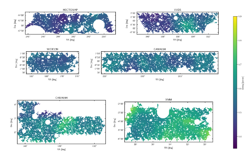
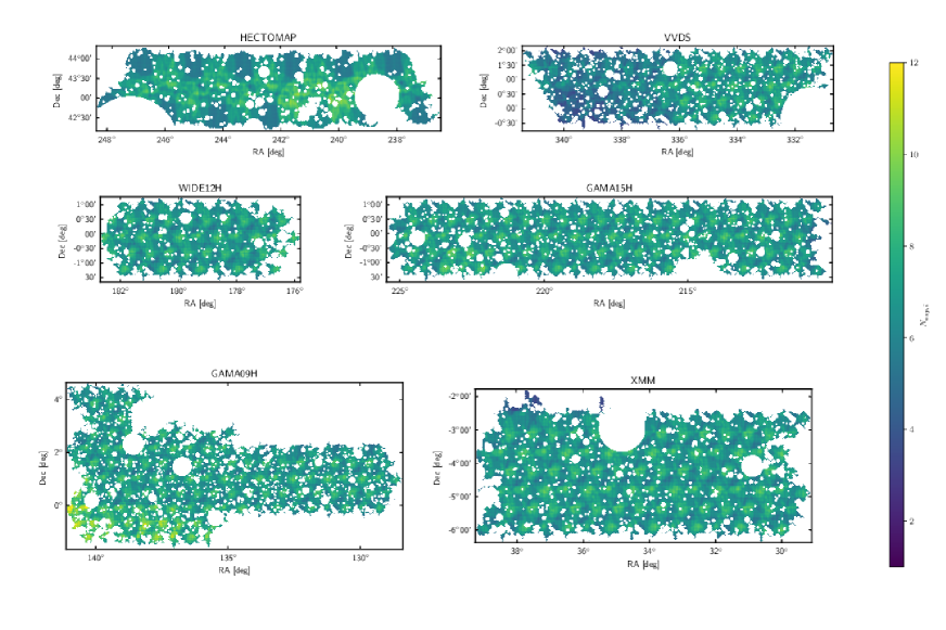
The data we use in this paper were taken during March 2014 through April 2016 with about 90 nights in total. Note that the publicly-released HSC DR1 data is based on data taken during March 2014 through Nov 2015 with a total of 61.5 nights. However, the same analysis pipeline was run on the 90 night dataset used for the shear catalog described in this work (as described in the HSC DR1, which mentions this internal data release), ensuring consistency of all aspects of image processing between the publicly-released subset of the data and the full catalog. Maps of the $i$-band PSF FWHM and number of $i$-band exposures across this 90-night dataset are shown in figures 1 and 2, and illustrate that the catalog covers six distinct fields that will hereafter be referred to as HECTOMAP, VVDS, WIDE12H, GAMA15H, GAMA09H, and XMM.

For the weak lensing shear catalog, we make a number of well-motivated cuts on this dataset:

• Weak lensing full depth and full color (WLFDFC) cut: We restrict ourselves to regions that reach the approximate full depth of the survey in all 5 broadband filters ($grizy$), to achieve better uniformity of the shear calibration and photometric redshift quality across the survey. This cut is non-trivial mainly because of issues like chip gaps which could result in lattice-like features in the area coverage depending on how the cut is applied. In detail, this cut is imposed by requiring the number of visits within HEALPix pixels with NSIDE=1024 to be $(g,r,i,z,y)\geq(4,4,4,6,6)$ and $i_{\rm lim}>25.6$ (using a limiting magnitude definition described below). We allowed the $i$-band number of exposures to be smaller than the ideal value (6) so as to avoid removing part of the VVDS field where visits with excellent seeing (resulting in poor PSF modeling as described in the HSC DR1 paper) were removed from the coadds. Given the very good seeing, the limiting magnitude can nevertheless meet our target.

  The limiting magnitude is estimated as follows. First we obtain a limiting magnitude for each patch from the database. This limiting magnitude is defined as the magnitude at which the PSF photometry has $S/N\sim 5\sigma$ (for details, see the HSC DR1 paper). However, we cannot immediately use this limiting magnitude because it fails in some patches due to the failure of forced measurements. Instead, we perform a linear fit on the limiting magnitude as a function of seeing, which is again obtained from the database, and the number of visits (ignoring the dependence on transparency), and use this linear fit for the limiting magnitude in all the patches. Note that this WLFDFC cut is defined differently from the full depth cut in the HSC DR1 paper, with the most important difference being that it is more inclusive in the VVDS field in regions where some exposures were removed.

• PSF model failures: as detailed at the start of Section 4, we eliminate regions with demonstrable PSF modeling failures in the coadd PSF (defined in Section 2.3) according to a cut given in that section.

• We remove disconnected regions created by the above two cuts in the HEALPix pixelization, in order to obtain a contiguous survey area.

• We require that the galaxies not lie within the bright object masks (which will be described in Section 2.3).

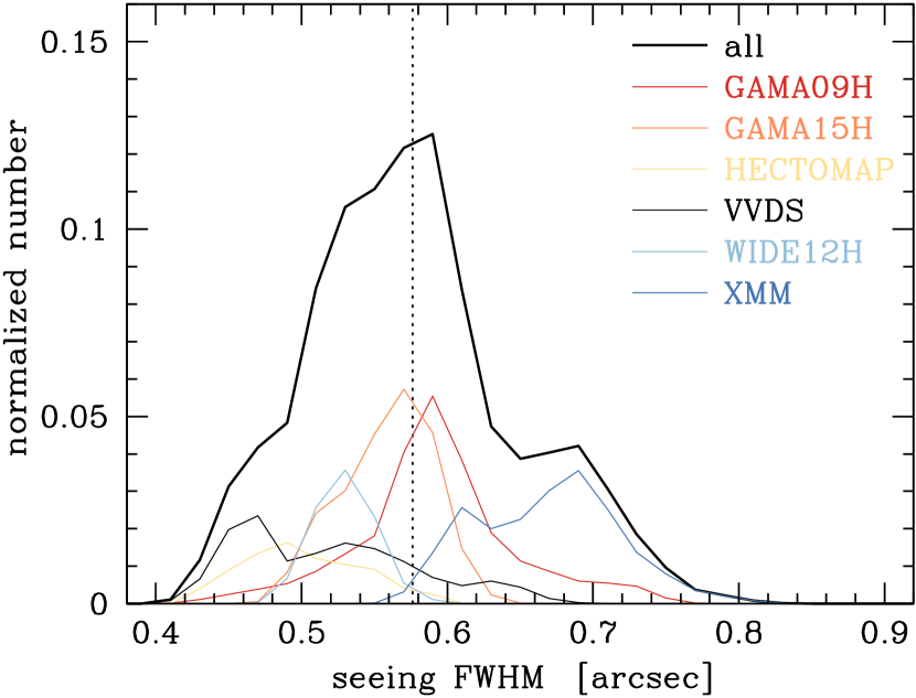
After these cuts, the total area of the catalog is 136.9 deg². As shown in figure 1, the best-seeing fields are HECTOMAP and VVDS, while WIDE12H and GAMA15H are around the median value of seeing, GAMA09H has some areas that are worse than the median, and XMM has clearly the worst imaging conditions. Not surprisingly given the imposition of cuts to achieve approximately full depth in all filters, the regions all have a fairly similar number of contributing exposures (figure 2). The slight deficit in VVDS is a result of data processing (removing exposures in which PSFs could not be modeled well, see introduction to Section 4) rather than observations. Figure 3 shows the distribution of $i$-band PSF FWHM values for the objects in the shear catalog.

Figure 3: Unweighted histogram of the $i$-band PSF FWHM values for galaxies in the shear catalog across each field and overall. The vertical dotted line indicates the average PSF FWHM value of $\sim 0.58$.

2.3 HSC software pipeline

The processing of single frame HSC images is described in detail in Bosch et al. (2017). We only mention here the details of hscPipe that are important for weak lensing measurements. Also, the software is constantly evolving; this paper describes a snapshot of it as of the time these data were processed, hscPipe v4.0.2, though the photometric redshifts rely on subsequent processing of the photometry from v4.0.3 as described in Tanaka et al. (2017).

We utilize software being developed for the Large Synoptic Survey Telescope (LSST; Axelrod et al. 2010; Jurić et al. 2015). Basic routines are performed to remove the signature of the instrument including flat-fielding, bias subtraction, correction of non-uniformity of plate scale, removal of bad pixels, and so on. Measurement and detection of objects occurs in two phases. The first phase only measures the brightest objects ($S/N\gtrsim 50$) to characterize the PSF separately for each CCD and do an initial astrometric and photometric calibration. From this initial bright object catalog, we select potential star candidates for PSF estimation by looking at clustering in size. We use a k-means clustering algorithm which iteratively assigns objects to the cluster with the closest mean. We have found that fixing the number of clusters to four and identifying star candidates as the cluster with the smallest average size has worked reasonably well. We typically select $\sim 80$ star candidates per CCD.

2.3.1 PSF modeling

The selected stars are fed into the PSFEx (Bertin, 2011) package to model the position-dependent PSF. We altered PSFex so that it could be used as an external library in the LSST software, independent of SExtractor. Currently, we reserve 20$\%$ of the stars as a cross-validation sample and do not use them in the modeling. The PSF model is constructed in the native pixel basis and we use a second order polynomial per CCD for interpolation. Using a higher order polynomial is not worth the cost of the extra parameters, as it was found to produce only minor improvements in some CCDs at the focal plane edge.

2.3.2 The brighter-fatter effect

We also apply a correction to account for the brighter-fatter effect (Antilogus et al., 2014; Gruen et al., 2015). Charge that enters the detector is deflected by a lateral electric field due to accumulated charge in the pixel. This alters the drift lines pushing some of the charge to land in adjacent pixels, thus causing bright stars to appear slightly larger than faint ones. Ignoring this effect will cause the PSF used for determining faint galaxy shapes to be incorrect. We use an algorithm to revert this effect (Coulton et al., in prep.) where we assume the lateral electric field is curl-free and can be written as the gradient of a kernel that is translationally invariant and proportional to the accumulated charge. We construct this kernel from flat-field images. After applying this correction, the dependence of PSF model size on magnitude is reduced below the scientific requirements (see figure 6, top right panel).

2.3.3 Coaddition process

For our first-year science analysis, all measurements of galaxies in HSC are performed on coadded images, including shear estimation. Coaddition is performed without PSF homogenization (PSF matching of different exposures); instead we extend the “StackFit” approach of Jee & Tyson (2011) by computing the effective PSF on the coadd at the position of each galaxy from the PSF models of the input images rather than from the coadd itself (see also Annis et al., 2014). Because convolution is a linear operation and we have applied the same coordinate transformations and weights to the PSFs and the input images, the PSF on this coadd (“coadd PSF”) can theoretically be predicted exactly (aside from astrometric registration errors, which also affect non-coadd measurements), but will be discontinuous in regions where the set of input images changes. Because our measurements assume that the PSF is constant over the scale of individual objects, we do not attempt to include the effect of small-scale changes in the input image set due to masked pixels on input images (e.g., cosmic rays or bad columns) in the PSF. Instead, we simply mask the regions of the coadd for which the set of input images is not constant across detected objects, and reject galaxies that overlap these regions from our sample. Null tests of the PSF models are performed on the coadd to ensure that the stacked PSF models adequately describe the coadd PSF (Section 4).

This approach to coaddition also requires a strictly linear combination of images (i.e., a weighted mean). Using per-pixel robust estimation or outlier rejection (such as a median or sigma-clipping) to combine images with different PSFs would not merely invalidate our PSF estimation approach – they would ensure that the coadd does not have any well-defined PSF at all, because different input images would be systematically clipped in the cores and wings of objects. To reject artifacts such as cosmic rays and saturated pixels from images, we instead identify the actual artifacts on the input images, using the following procedure:

1. We build a preliminary coadd with no outlier rejection.

2. We build a second preliminary coadd using strong outlier rejection (mean with iterative 3-sigma clipping).

3. We subtract the two preliminary coadds and threshold to find pixels at which they differ.

4. We monitor the input images for each such region in an automated way, and keep only regions where one or two input images contributed to the difference.

5. We expand each region on each of the input images that contributed to it to include all simply-connected pixels above some threshold.

6. We build a new coadd with no outlier rejection, with the input image regions defined above ignored and these locations masked on the final coadd. The coadded PSF models do not take into account pixels that are ignored in this manner and hence are subtly incorrect in these regions.

These coadd masks are then used to filter the galaxy catalog, ensuring that it does not include any objects for which the PSF model is incorrect due to rejected pixels.

2.3.4 Detection and deblending

Coadds for different bands are built independently, and detections (above-threshold regions and peaks within them) are identified separately in each band. We then merge the detections across all bands, merging co-located peaks to eliminate redundant detections and computing new above-threshold regions as the union of the per-band region. Each simply connected region is considered a family of blended objects. We then independently deblend and measure in each band. This deblending takes the number of objects in each family and their approximate positions as fixed from the previous step, ensuring that these per-band measurements are broadly consistent, but we currently do not otherwise ensure that per-pixel assignments of flux to deblended child objects are consistent across bands. This approach to deblending is likely to change in future versions of the software pipeline.

2.3.5 Measurement algorithms

The measurement algorithms run at this stage include centroiding, shape measurement, and PSF, galaxy model, Kron, and aperture fluxes. After measurement, we select a “reference” band for each object, using the $i$ band for all objects with $S/N>10$ and falling back to other bands as necessary in the order $r$, $z$, $y$, $g$. Measurements in the reference band are then used to drive another round of per-band “forced” measurements, with centroids and shapes held fixed at the values from the reference band. Fluxes measured in this forced mode are used to compute colors and photometric redshifts.

2.3.6 Bright object masks

Bright stars affect galaxy detection and photometry most notably through the luminous PSF pattern, ghosting, and by altering the local sky background. We mask all stars that saturate the typical exposures, accounting for the fact that the saturation limit depends on the filter and on the observing conditions (such as transparency and seeing). To do so, we use a sample of bright stars that is complete in all optical bands down to ${\rm mag}<17.5$. This conservative limit, estimated from PSF magnitudes in each HSC band, ensures that all saturated stars in our survey are properly masked (at the expense of a small fraction of non-saturated stars that are also masked). We note that these masks are only used to remove sources from the shape catalog that are located near a bright object, however, they were not used at any other step during data processing.

We first use the Tycho-2 star catalog (Høg et al., 2000) to identify all bright stars in our fields, and supplement this with the NOMAD catalog (Zacharias et al., 2004) at fainter magnitudes ($10.0<{\rm minimum}(B,V,R)<17.5$), which is a compilation of a number of all-sky star catalogs. The main caveat of the NOMAD catalog is that it is contaminated by a small fraction of bright galaxies (visual inspection suggests that about 10% of the objects are galaxies). Given this contamination by galaxies, the masks will be called bright object masks from now on. We note that masking galaxies brighter than $17.5$ has no impact on the galaxy shape catalog, composed of much fainter sources, however, we warn that any other science analysis making use of galaxies brighter than $17.5$ in any band should not use the bright object masks. This caveat about inclusion of bright galaxies from the NOMAD catalog is valid for the bright object masks used here, which were an early version called ‘Sirius’. The version described in Coupon et al. (2017) and called ‘Arcturus’ are updated to remove the bright galaxies, and so are called ‘bright star’ rather than ‘bright object’ masks. The updated version, which is suitable for use in a broader range of science cases, will be included in subsequent data releases.

To build individual masks, we characterize, per bin of bright-object magnitude, the radial extent to which bright objects affect neighbouring source counts by measuring the two-point cross-correlation function between bright stars and all HSC detected sources (without any cut on the pipeline flags). At small radius, we observe a rapid decrease in the density of detected sources. At large radius, however, we observe an enhancement of detected sources; the luminous halo of the bright object boosts the local background and leads to an increased number of noise detections. This feature is more prominent for faint detections but occurs around the same radius, for a given bright object magnitude, regardless of the detected source magnitude. We conservatively use the position of this feature to set the extent of the mask. The size of the mask is kept fixed across the five HSC filters and the reference bright-object magnitude ($m_{\rm BS}$) is chosen to be the brightest of the optical magnitudes provided by each respective catalog, $B$, $V$, and $R$ from the NOMAD catalog and the SDSS-emulated $g$, $r$ and $i$ (Pickles & Depagne, 2010) from the Tycho-2 catalog. For each bright object, we build a circular mask whose radius depends on the bright-object magnitude ($m_{\rm BS}$) according to:

$$r_{\rm{mask}}\,\mathrm{[arcsec]}=200\times 10^{0.25(7.0-m_{\rm BS})}+12\times 10^{0.05(16.0-m_{\rm BS})}\,,$$ (1)

where the parameters reproduce the measured radius at which the source detection near the bright object starts to feature an enhancement. The total masked area due to bright objects in the WLFDFC region is 16%. We note that equation (1) diverges at bright magnitudes, and as a result significantly overestimates the size of the required mask for a few very bright stars (mag$<4-5$). This problem is also updated in the mask version described in Coupon et al. (2017).

2.4 Shear estimation algorithm

Since the initial development of algorithms for estimating shear that correct for the effects of the PSF on galaxy images using measurements of moments of the PSF and galaxy shape (e.g., Kaiser et al., 1995), the field has seen tremendous development in the variety and accuracy of methods. This evolution has been demonstrated through a series of community challenges (Heymans et al., 2006; Massey et al., 2007b; Bridle et al., 2009, 2010; Kitching et al., 2010, 2012; Mandelbaum et al., 2014, 2015). In the most recent of these, GREAT3, the types of methods used included those based on estimation of per-galaxy shapes via measurements of moments, fitting parametric light profiles, decomposition into basis functions, and machine learning, as well as methods that involve inferring ensemble shears without per-galaxy shapes. The majority of methods that are actively used for weak lensing science achieved multiplicative bias in the $\lesssim 2$% range, meaning that for a true ensemble shear $g$ the estimated ensemble shear $\hat{g}=(1+m)g$ for a multiplicative bias $|m|\lesssim 0.02$. As we will show in Section 3, these methods would meet the requirements for first-year weak lensing science with HSC, but not necessarily full HSC survey science requirements.

There are a number of important issues for shear estimation methods that are based on averages of per-galaxy shape estimates. One of these is “noise bias” (e.g., Bernstein & Jarvis, 2002; Hirata et al., 2004; Kacprzak et al., 2012; Melchior & Viola, 2012; Refregier et al., 2012), wherein the pixel noise modifies the shape of the likelihood surface and causes the maximum-likelihood estimator of per-galaxy shapes to be biased. Another is “model bias”: a number of studies have convincingly demonstrated that when estimating shears using a method that assumes a particular galaxy model, the shears can be biased if the galaxy light profiles are not correctly described by that model (e.g., Voigt & Bridle, 2010; Melchior et al., 2010). More generally, any method based on the use of second moments to estimate shears cannot be completely independent of the details of the galaxy light profiles, such as the overall galaxy morphology and presence of detailed substructure (Massey et al., 2007a; Bernstein, 2010; Zhang & Komatsu, 2011). Selection biases, for example due to the selection criteria correlating with the lensing shear or PSF anisotropy, also play an important role (e.g., Hirata et al., 2004; Jarvis et al., 2016). In general, these basic mathematical issues in estimating shear from per-galaxy shapes require either external calibration using simulations, or some form of self-calibration (e.g., Fenech Conti et al., 2017; Huff & Mandelbaum, 2017; Sheldon & Huff, 2017). An alternative is to use a method that is designed to infer an unbiased estimate of the ensemble shear but not necessarily (or at all) an unbiased estimate of per-galaxy shapes (Bernstein & Armstrong, 2014; Schneider et al., 2015; Bernstein et al., 2016).

The first year shear catalog for HSC weak lensing was produced using a moments-based shape measurement method for which the shear is estimated by averaging the shapes, described below; for this method, we use suites of simulations (Section 6.2) to remove the aforementioned forms of biases to which the method is naturally prone. A forthcoming paper (Armstrong et al., in prep.) will describe a catalog produced using a Bayesian ensemble shear inference method (Bernstein et al., 2016; Bernstein & Armstrong, 2014).

Galaxy shapes are estimated on the coadded $i$-band images using the re-Gaussianization PSF correction method (Hirata & Seljak, 2003). This method was extensively used and characterized for science in the Sloan Digital Sky Survey (SDSS; Mandelbaum et al. 2005; Reyes et al. 2012; Mandelbaum et al. 2013), and then incorporated into the GalSim (Rowe et al., 2015) open-source software package after further optimization for speed. The HSC pipeline relies on the GalSim implementation of this algorithm.

The basic principle of galaxy shape estimation using this method is to fit a Gaussian profile with elliptical isophotes to the image, and to define the components of the distortion

$$(e_{\mathrm{1}},e_{\mathrm{2}})=\frac{1-(b/a)^{2}}{1+(b/a)^{2}}(\cos 2\phi,\sin 2\phi),$$ (2)

where $b/a$ is the axis ratio and $\phi$ is the position angle of the major axis with respect to the equatorial coordinate system (sky coordinates). In the course of the re-Gaussianization PSF-correction method, corrections are applied to account for dilution of the observed shape by the PSF, including the non-Gaussianity of both the PSF and the galaxy surface brightness profiles (Hirata & Seljak, 2003). The ensemble average distortion is then an estimator for the shear $g$,

$$(\hat{g}_{\mathrm{1}},\hat{g}_{\mathrm{2}})=\frac{1}{2\cal R}\langle(e_{\mathrm{1}},e_{\mathrm{2}})\rangle,$$ (3)

where ${\cal R}$ is called the ‘shear responsivity’ and represents the response of the distortion (equation 2) to a small shear (Kaiser et al., 1995; Bernstein & Jarvis, 2002); ${\cal R}\approx 1-e_{\mathrm{rms}}^{2}$, where $e_{\mathrm{rms}}$ is the RMS intrinsic distortion per component. The equations used for the actual shear estimation process are given in Appendix C. The notation used in this paper is that shear components called $(1,2)$ are in sky coordinates, while those denoted $(+,\times)$ are in a coordinate system defined for pairs of objects. In that case $\hat{g}_{+}$ (tangential shear) is defined with respect to the vector connecting the pair and $\hat{g}_{\times}$ with respect to the axes rotated by $45^{\circ}$.

It is useful to be able to apply selection criteria based on how well-resolved the galaxy is compared to the PSF. For this purpose, we use the resolution factor $R_{2}$ which is defined using the trace of the moment matrix of the PSF $T_{\mathrm{P}}$ and of the observed (PSF-convolved) galaxy image $T_{\mathrm{I}}$ as

$$R_{2}=1-\frac{T_{\mathrm{P}}}{T_{\mathrm{I}}}.$$ (4)

Well-resolved objects have $R_{2}\sim 1$ and poorly resolved objects have $R_{2}\sim 0$.

The estimation of the shear responsivity in light of shape measurement errors that make it difficult to infer the intrinsic shape dispersion, and the exact selection criteria to place on the resolution factor and other galaxy properties, are discussed in Section 5.

2.5 Systematics analysis software

For our systematics tests we use the software Stile, Systematics Tests In LEnsing. It is open-source and publicly available, and was developed specifically to enable easy calculation of a wide range of null tests for a large-area lensing survey such as HSC.

The Stile code consists of a set of Python classes that perform systematics tests, plus ancillary code for data handling. The code used for this paper performs five main types of tests.

• The CorrelationFunctionSysTest. This acts as a wrapper for the software TreeCorr (Jarvis et al., 2004), performing different kinds of correlation functions with appropriate parameter values.

• The WhiskerPlotSysTest. This produces whisker plots of star and PSF ellipticities and their residuals.

• The ScatterPlotSysTest. This takes two columns of data and produces a scatter plot and optionally a fitted trendline.

• The HistogramSysTest, which produces histograms.

• The StatSysTest. This produces basic statistical quantities such as mean, median, and percentile rankings.

The CorrelationFunction, WhiskerPlot, and ScatterPlotSysTests all have predefined systematics test types (such as the $\rho$ statistics, equations (26)–(30), for the CorrelationFunctionSysTest and whisker plots of the PSF-star residuals for the WhiskerPlotSysTest). Additional tests can be added by making subclasses of the existing tests, without much unnecessary overhead. The existing tests handle details such as forming residuals or other combinations of parameters if necessary, finding automatic bin widths for the histograms, and fitting trendlines to scatter plots. They also have plotting routines if applicable, though we used specially-created plotting routines for the plots in this paper, rather than Stile defaults (which do not currently allow us to plot multiple fields at once).

TreeCorr (Jarvis, 2015) is a fast correlation function code that uses a ball tree method (similar to a k-d tree). In this work we use its methods for point-shear correlation functions $\langle g\rangle$ (TreeCorr type ‘ng’), shear-shear correlation functions $\langle g\,g\rangle$ (TreeCorr type ‘gg’), and scalar-scalar correlation functions $\langle\kappa\kappa\rangle$ (TreeCorr type ‘kk’).

The Stile tests operate on Python data arrays that can be accessed by column name. A unified set of column names is expected, but the data can otherwise be in any format. The Stile code also has the ability to interface with the LSST/HSC pipeline; we used this functionality during early data processing but not in the final versions of the tests presented here, which used versions of catalogs that have all weak lensing selection criteria applied.

More detailed information (including calculation details and usage instructions) can be found in the package documentation on GitHub.

3 Requirements

Before presenting the results of systematics tests, we need to define the requirements for the catalog to enable first-year HSC weak lensing science. For the purpose of setting requirements, we consider two cosmological measurements as the goal of first-year HSC weak lensing science: the shear-shear correlation function using the entire shear catalog (no tomography), and the galaxy-shear correlation function (i.e., galaxy-galaxy lensing) using the SDSS-III/BOSS (Dawson et al., 2013) CMASS sample (Reid et al., 2016). The latter will be combined with galaxy clustering measurements to enable cosmological parameter constraints, as an alternate cosmological method to cosmic shear. For this paper, the calculations for setting requirements involve (a) estimating statistical errors in the fiducial weak lensing analyses for the first-year HSC data; (b) assessing how systematic errors propagate into cosmological observables; (c) comparing those systematic errors to the statistical errors; and (d) requiring each systematic error to contribute below some fraction of the statistical errors. In principle, one can set requirements by doing the full forecasting of how those systematics in the cosmological observables propagate into systematics on cosmological parameter constraints (e.g., Jarvis et al., 2016). We did not adopt that approach in this paper, though we do present estimates of how our requirements, as currently calculated, propagate into cosmological parameter constraints. The overall process described here is broadly consistent with that used for several ongoing and future surveys (Amara & Réfrégier, 2008; Massey et al., 2013; Jarvis et al., 2016; Hildebrandt et al., 2017), differing only in small details of the implementation.

In the following we will often assess the requirements in terms of “multiplicative” and/or “additive” biases in shear estimation, which are defined as $\hat{g}=(1+m)g^{\rm true}+c$, respectively (Mandelbaum et al., 2015). Some systematic errors, such as those that induce additive biases in shears, only contribute to cosmic shear. Others, such as multiplicative biases in the shear, affect both cosmic shear and galaxy-galaxy lensing. In that case, we assess the requirements on the systematic separately for both measurements, and adopt the more stringent requirement. We will also consider additive and multiplicative biases to be completely uncorrelated and hence constrain the two separately. In practice, selection biases or other effects could couple these, but we expect this to be a higher-order effect that is not of concern in first-year HSC analysis.

In this context, the word “requirements” has a very specific meaning: the requirements are defined such that if a systematic requirement is met, then the systematic is small enough that it can be ignored as part of the error budget in a science analysis. If one of our systematic requirements is not met, then it does not mean science cannot be done; rather, it means that the systematic is not small enough compared to our statistical errors that we can safely ignore it, but rather needs to be explicitly accounted for (e.g., modeled and marginalized over) in a way that shows that it is a non-negligible portion of the error budget. It is the goal of this paper to check for the various types of systematics that can affect weak lensing analyses, and classify them as ones meeting requirements (subdominant part of the error budget) versus those that are similar in magnitude to or exceeding our requirements, requiring further work to explicitly account for them in a science analysis. For those systematics that can be detected using null tests, we carry out those tests; for others, we describe how the systematic is tested in a separate paper (if requiring external simulations or data). Future science papers can then start with a focus on the small subset of problems that are identified as important for that science case in this work.

In general, we require that systematic uncertainties be limited to $\lesssim 0.5\sigma$ of the statistical errors on the measurements. Note that these are requirements on the systematic uncertainties, not biases. Known biases should be removed from the measurements before using them for science. The choice of a $\lesssim 0.5\sigma$ threshold for defining requirements is somewhat arbitrary. Ultimately for any science analysis, both statistical and systematic errors must be reported and used to assess the relative importance of systematics. If the science case differs from the examples used in this section, a potentially lower $S/N$ could justify a higher tolerance for systematic uncertainty. However, we use this $0.5\sigma$ threshold as a way of asserting that in general, for our highest-$S/N$ cosmological science cases, our goal is for statistical error to dominate over systematic error. If statistical and systematic errors are independent and add in quadrature, then this $0.5\sigma$ threshold would mean that the systematic errors inflate the overall (total statistical $+$ systematic) error budget by 12 per cent.

The connection between systematics requirements and statistical errors also means that the requirements become more stringent once more of the survey is complete. A rough estimate of the final requirements (without accounting for details of survey edge effects) is that they will be a factor of $\sim 2.7$ times tighter than the ones presented in this work. We do not compare our current estimates of systematic uncertainties with the tighter, full-survey requirements because the HSC pipeline as described in Bosch et al. (2017) will be evolving in certain ways that are highly relevant to weak lensing, e.g., adoption of improved PSF modeling and shear estimation routines, so our current results are irrelevant to the full survey dataset. However, this factor of $\sim 2.7$ can be helpful to bear in mind when identifying important directions for future work.

Note that there are many sources of multiplicative bias in shear estimates. When discussing multiplicative bias in the subsections below, we will derive a constraint on the uncertainty in the shear calibration (after correcting for known calibration biases) across all of these sources of error: star/galaxy separation failure (i.e., stellar contamination of the galaxy sample); PSF model size errors; shear-related biases like model bias, noise bias, and selection bias; and photometric redshift biases. In general, our constraints are on the uncertainty in the component-averaged shear calibration. While many methods of shear estimation exhibit a slight difference in calibration bias for the component that is along vs. diagonal compared to the pixel direction, any practical shear measurement involves an average over those two components, so we place requirements on the systematic uncertainty of the average.

3.1 Covariances

An important part of setting requirements is understanding the statistical errors in the relevant measurements. Overly optimistic statistical uncertainties due to neglecting important error contributions will result in overly stringent requirements on systematics, which may be difficult to meet in practice. To account for all important sources of error in shear-shear correlations (including galaxy shape noise, cosmic variance, and super-sample covariance) and in galaxy-shear correlations (including the above, plus lens shot noise error terms) (Takada & Hu, 2013), we use mock galaxy catalogs that include various effects: properties of source galaxies, lensing effects on each source galaxy due to the foreground large-scale structure (cosmic shear), weights, and the survey geometry. These are catalog simulations rather than image simulations, but the impact of shape noise and measurement error due to noise in the images is included properly as described below. Here we briefly summarize the mock catalogs of HSC data, which we will use to derive requirements on shape measurements for the science analysis with the shape catalog described in this paper. More detailed descriptions of mock catalogs will be presented in Shirasaki et al. (in prep.).

We first describe the mock shear catalogs of HSC source galaxies. We follow the method developed in Shirasaki & Yoshida (2014) (also see Shirasaki et al., 2017) to perform ray-tracing on a large number of cosmological light-cone simulations. We generate $48$ full-sky light-cones using outputs of different box-size $N$-body simulations for the nine-year WMAP cosmology (Hinshaw et al., 2013). For details of the cosmological parameters and $N$-body simulations, see also Shirasaki et al. (2017). We used the multiple-lens plane algorithm on the sphere to simulate the light-ray path and lensing of a source galaxy by the structure along its line-of-sight. The ray-tracing simulations are designed to simulate the weak lensing effect on source galaxies at different redshifts, over a full sky given in the HEALPix format of 0.43 arcmin pixel scale. Although the original $N$-body simulations have a higher resolution, we use this pixel scale because we use this mock catalog to estimate the covariance matrix of lensing observables. The covariance at scales smaller than this pixel scale is dominated by shape noise or shot noise, which we account for by preserving pairs of two source galaxies or lens-source galaxies at scales below the HEALPix pixel scale in the galaxy-galaxy lensing calculation.

The simulation consists of 38 different source planes each separated by a comoving separation of $\Delta\chi=150\,h^{-1}{\rm Mpc}$, thus covering source planes up to redshift $z_{s}\simeq 5.3$. The angular resolution and the redshift coverage are suitable for our purpose of creating mock catalogs for the first-year data of HSC. We incorporate our simulations with observed photometric redshifts and angular positions of $real$ galaxies. In brief, (1) we insert each galaxy, taken from the real HSC catalog, into the nearest angular pixel in the nearest redshift source plane, (2) we randomly rotate the orientation of its shape to erase the real lensing effect, and (3) we simulate the lensing distortion effect on the source galaxy by adding the lensing shear and the intrinsic shape, and (4) repeat the procedures (1)–(3) for all the source galaxies. Note that, for every realization, we randomly sample the source redshift from the posterior probability distribution of photometric redshift for each galaxy. Thus, our mock catalogs include effects of properties of source galaxies (e.g., magnitudes, ellipticities and spatial variations in the number densities), statistical uncertainties in photometric redshifts as well as the survey geometry. Since the six HSC S16A regions are separated from each other as shown in figures 1 and 2, we generate 21 different mock catalogs from 21 different rotations of the spherical coordinates preserving the relative positional locations of the HSC S16A fields on the sky. This allows us to generate 21 independent mock catalogs from each full sky simulation without overlap. This results in a total of 1008 realizations of HSC mock shear catalogs, generated from the 48 full-sky lensing simulations.

In what follows, we will also derive requirements on the level of residual systematic errors for galaxy-galaxy weak lensing. For this purpose, we create mock catalogs of CMASS galaxies, which are our primary targets for the galaxy-galaxy lensing measurements, based on the halo occupation distribution (HOD) approach. To do this, we use the catalog of halos that are built from the same $N$-body simulation outputs used for the ray-tracing simulations. To identify halos in each $N$-body simulation output, we used the software Rockstar (Behroozi et al., 2013) that identifies halos from the clustering of $N$-body particles in phase space. Our $N$-body simulations allow us to resolve dark matter halos with masses greater than a few times $10^{12}h^{-1}\,M_{\odot}$ with more than 50 $N$-body particles at redshifts $z\lower 2.15277pt\hbox{$\;\buildrel<\over{\sim}\;$}0.7$, which cover the range of redshifts of CMASS galaxies. We assign three-dimensional positions for all halos (angular position and redshift) in the light cone depending upon their positions in the $N$-body simulation output.

We populate galaxies in these dark matter halos with an HOD that is constrained based on the number density and spatial clustering of CMASS galaxies in the redshift range $z\in[0.43,0.55]$ and $z\in[0.55,0.7]$ but spanning the entire SDSS BOSS footprint. We constrain a simple 5 parameter HOD (see e.g, White et al., 2011) based on the analytical modelling framework developed in van den Bosch et al. (2013). This HOD is used to populate mock CMASS galaxies in the halos of the light cone. This galaxy catalog in conjunction with the source catalog output from the same light-cone are then used to perform 1008 mock measurements of galaxy-galaxy weak lensing. These measurements are then used to compute a covariance matrix.

3.2 Requirements for galaxy-galaxy lensing

For galaxy-galaxy lensing (hereafter abbreviated “g-g”), it is possible to remove additive systematics in the shear via cross-correlation with a random catalog that has the same area coverage as the lens sample (e.g., Mandelbaum et al., 2013). As a result, we are primarily concerned with placing requirements on systematics that cause a systematic uncertainty in the overall amplitude of the shear. We will place two requirements in this section:

• an overall requirement on uncertainty in the shear calibration (across all sources of multiplicative bias, as described in the introduction to this section) to achieve our goal of having it contribute at $<0.5\sigma$ in all bins in CMASS galaxy-galaxy lensing with the first-year shear catalog, and

• a more specific and more stringent requirement that systematic uncertainty due to PSF modeling errors alone contribute at $<0.25\sigma$. Here the relevant PSF modeling errors are PSF size errors, which propagate into a multiplicative shear bias.

3.2.1 Multiplicative bias in shear

To place a requirement on systematic uncertainty due to any source of uncorrected multiplicative bias in the shear for CMASS galaxy-galaxy lensing, we consider the expected fractional uncertainty in the lensing signal $\Delta\Sigma$. In particular, given a data vector $\vec{x}$ consisting of the predictions for $\Delta\Sigma$ in bins of projected separation $r_{p}$ from the CMASS galaxies, and the expected covariance matrix from the mock catalogs $\mathbf{C}$, we can define the total SNR for CMASS galaxy-galaxy lensing as

$$\text{SNR}_{\text{g-g}}=[\vec{x}^{T}\cdot\mathbf{C}^{-1}\cdot\vec{x}]^{1/2}.$$ (5)

We obtain $\text{SNR}_{\text{g-g}}=29.9$ on scales from 0.5–30$h^{-1}$Mpc for the sample of CMASS galaxies from $z\in[0.43,0.7]$, including CMASS galaxies in BOSS regions covering a wider area surrounding each HSC field. We require the overall uncertainty in the shear calibration allowed for CMASS g-g lensing, $|\delta m_{\text{all-g-g}}|$, to be below $0.5/\text{SNR}_{\text{g-g}}$, thus,

$$|\delta m_{\text{all-g-g}}|<\frac{0.5}{\text{SNR}_{\text{g-g}}}=0.017\,.$$ (6)

3.2.2 PSF model size errors

Here we want to place a more specific requirement on systematic uncertainty due to coherent PSF model size errors, which can be considered a source of shear calibration uncertainty $|\delta m_{\text{PSF-g-g}}|$ that we would like to be less than half the overall shear calibration uncertainty budget, $|\delta m_{\text{PSF-g-g}}|<0.5|\delta m_{\text{all-g-g}}|$ or $0.25/\text{SNR}_{\text{g-g}}$. In other words, we need to leave some of the overall calibration budget for other sources of systematics that cause multiplicative bias in shear besides the PSF model size errors. We then need to relate $|\delta m_{\text{PSF-g-g}}|\lesssim 0.5|\delta m_{\text{all-g-g}}|$ to some statistic that we can measure from the catalog, in order to place a requirement on that statistic.

In this case, we can use the formalism from Hirata et al. (2004), who show that the shear calibration uncertainty for a given PSF model size error for a galaxy of resolution factor $R_{2}$ is

$$\delta m_{\text{PSF-g-g}}(R_{2})=-\left(R_{2}^{-1}-1\right)\frac{T_{*}-T_{\text{PSF}}}{T_{\text{PSF}}}.$$ (7)

Here, $T_{*}$ and $T_{\text{PSF}}$ are the trace of the second moment matrix of stars and PSFs. Well-resolved objects ($R_{2}$ near 1) are minimally affected by PSF model errors, while this systematic becomes very large as $R_{2}$ approaches zero. To relate this to quantities that we measure, we first consider that the fractional error in the trace (which is a measure of area) is double that of the linear size $\sigma$ which we use to quantify PSF model size errors. We furthermore place a constraint on the average PSF model size error, because stochastic errors in PSF model sizes will average out and will not cause a bias in galaxy-galaxy lensing. Hence

$$\langle\delta m_{\text{PSF-g-g}}(R_{2})\rangle=-2\left\langle\left(R_{2}^{-1}-1\right)\frac{\sigma_{*}-\sigma_{\text{PSF}}}{\sigma_{\text{PSF}}}\right\rangle,$$ (8)

and asserting the independence of galaxy properties like $R_{2}$ and PSF model properties, we can average over those properties separately:

$$\langle\delta m_{\text{PSF-g-g}}(R_{2})\rangle=-2\left\langle R_{2}^{-1}-1\right\rangle\left\langle\frac{\sigma_{*}-\sigma_{\text{PSF}}}{\sigma_{\text{PSF}}}\right\rangle.$$ (9)

As will be described later, our catalog has a lower limit of $R_{2}=0.3$. The weighted mean of $R_{2}^{-1}-1$ over the whole catalog is $0.8$. However, we would also like our requirements to be met by sub-populations of the catalog selected by e.g., photometric redshift or magnitude, so we will conservatively use a value of $\left\langle R_{2}^{-1}-1\right\rangle=1.0$ when placing the requirement. So we will require

$$\left\langle\frac{\sigma_{*}-\sigma_{\text{PSF}}}{\sigma_{\text{PSF}}}\right\rangle<\frac{|\delta m_{\text{PSF-g-g}}|}{2}\,\,\,<\,\,\,\frac{|\delta m_{\text{all-g-g}}|}{4}<0.004.$$ (10)

3.3 Requirements for cosmic shear

For cosmic shear, we care about both additive and multiplicative shear biases, including their spatial correlation function. We will place several requirements in this section:

• an overall requirement on shear calibration uncertainty (from all sources of multiplicative bias, as described in the introduction to this section) to achieve our goal of having it contribute at $<0.5\sigma$ in cosmic shear with the first-year shear catalog (Section 3.3.1),

• a more specific and more stringent requirement that calibration uncertainties due to PSF size modeling errors contribute at $<0.25\sigma$ (Section 3.3.2),

• a requirement that the systematic uncertainty due to overall additive biases from all sources (PSF shape errors, selection biases, insufficient correction for PSF anisotropy) are sufficiently small to ensure that the resulting additive bias term contributes at $<1\sigma$ on all scales (Section 3.3.3), and

• a requirement that the uncertainty on the PSF shape errors and their spatial correlation are sufficiently small to ensure that the resulting additive bias term contributes at $<0.5\sigma$ on all scales (it can be removed, but we do not want to be making very large corrections to the signal) in Section 3.3.4.

3.3.1 Multiplicative bias in shear

Following a similar methodology as in Section 3.2.1, we place requirements on the shear calibration uncertainty (from all sources of bias) for cosmic shear measurements. We use the same formalism to define an effective SNR on the shear-shear (“s-s”) correlations without tomography ($\text{SNR}_{\text{s-s}}$). In this case we assume the observable quantity will be the shear correlation functions $\xi_{\pm}(\theta)$. Assuming we have per-object shear estimates $\hat{g}$ which for pairs of galaxies can be decomposed into components $\hat{g}_{+}$ and $\hat{g}_{\times}$, then $\xi_{\pm}$ can be defined as

$$\xi_{\pm}(\theta)=\langle\hat{g}_{+}\hat{g}_{+}\rangle\pm\langle\hat{g}_{\times}\hat{g}_{\times}\rangle.$$ (11)

Hence our data vector $\vec{x}$ consists of the $\xi_{+}$ and $\xi_{-}$ values in $\theta$ bins, and $\mathbf{C}$ is its covariance matrix. To avoid scales which could be affected by either baryonic effects or theoretical uncertainties in the matter power spectrum, we use $\xi_{+}$ and $\xi_{-}$ measurements on scales $\theta>4$ and $>40$ arcminutes, respectively (Abbott et al., 2016). For the maximum angular scales, we set $\theta_{\rm max}=285$ arcminutes. We have checked that the SNR is not very sensitive to values of $\theta_{\rm max}$ above $50$ arcminutes, due to the limited sizes of our fields.

With a multiplicative bias model that looks like

$$\hat{g}=(1+m_{\text{all}})g,$$ (12)

where $g$ and $\hat{g}$ are the true and estimated shear, then in the limit that $|m_{\text{all}}|\ll 1$, this bias primarily affects the shear-shear correlations as

$$\langle\hat{g}\hat{g}\rangle\approx(1+2m_{\text{all}})\langle gg\rangle.$$ (13)

We therefore require the overall value of $2|\delta m_{\text{all}}|$ (systematic uncertainty in shear calibration) to be $\lesssim 0.5/\text{SNR}_{\text{s-s}}$, or

$$|\delta m_{\text{all-ss}}|\lesssim\frac{0.25}{\text{SNR}_{\text{s-s}}}.$$ (14)

For the cosmic shear measurements, we obtain a SNR of $12.6$ from the simulations, which results in

$$|\delta m_{\text{all-ss}}|\lesssim 0.020.$$ (15)

Given that the SNR of the cosmic shear measurement is slightly less than half that of the SNR of the CMASS g-g lensing measurement, the requirements for the multiplicative bias uncertainty are slightly more stringent for g-g lensing than for cosmic shear. We adopt the requirement $|\delta m|<0.017$ throughout and omit the subscripts “all-ss” and “all-g-g” hereafter.

So far the discussion has focused on the question of how systematics contaminate the observable quantities, such as the shear correlation function. However, we can also check how $|\delta m|<0.017$ translates into a bias on cosmological parameter estimates. We do this for the case of cosmic shear over the adopted range of scales, when modeling statistical errors only – i.e., without marginalizing over systematic uncertainties that are commonly marginalized over, such as intrinsic alignments and baryonic effects on the matter power spectrum. In that sense, our results are somewhat conservative, since marginalizing over these other effects will increase the statistical error and thus our tolerance for systematic uncertainty in the shear signal. We do not consider additional data, such as priors from the Cosmic Microwave Background data. Our cosmological parameter set for this analysis is $(\sigma_{8},\Omega_{m},n_{s},\Omega_{b},\theta_{*})$ with wide top-hat priors, and we marginalize over the last three quantities while considering the best-constrained combination of $\sigma_{8}$ and $\Omega_{m}$, which is here denoted $S_{8}\equiv\sigma_{8}(\Omega_{m}/0.3)^{0.5}$. We find the expected $1\sigma$ statistical uncertainty on $S_{8}$ is $\sigma(S_{8})=0.029$. The bias on $S_{8}$ as a function of $|\delta m|$ is found to be

$$|\Delta S_{8}|=(9.3\times 10^{-3})\left|\frac{\delta m}{0.017}\right|=0.32\,\sigma(S_{8})\,\left|\frac{\delta m}{0.017}\right|$$ (16)

Hence our requirements threshold corresponds to a bias in $S_{8}$ that is subdominant to the statistical errors, as expected.

3.3.2 PSF model size errors

As shown in equation (3.17) of Jarvis et al. (2016), the additive shift in the shear-shear correlation function $\xi_{+}(\theta)$ due to PSF model size errors, $\delta\xi_{+}$, can be written as

$$\delta\xi_{+}=2\left\langle\frac{T_{\text{PSF}}}{T_{\text{gal}}}\frac{\delta T_{\text{PSF}}}{T_{\text{PSF}}}\right\rangle\xi_{+}(\theta).$$ (17)

Here $T_{\text{gal}}$ is the trace of the second moment matrix of the galaxy itself (before PSF convolution). For the purpose of placing requirements, we use the theoretical model for $\xi_{+}(\theta)$ given the HSC redshift distribution. We also assert the independence of the first fraction (related to the typical galaxy resolution) and the second fraction (related to the PSF model size errors). As before, we set $\langle R_{2}^{-1}-1\rangle=1$ to place requirements, corresponding to $\langle T_{\text{PSF}}/T_{\text{gal}}\rangle=1$, and again set the fractional PSF model area error to twice the fractional PSF radius error. This gives

$$\delta\xi_{+}=4\left\langle\frac{\delta\sigma_{\text{PSF}}}{\sigma_{\text{PSF}}}\right\rangle\xi_{+}(\theta).$$ (18)

We would like to constrain this potential additive error to be $\lesssim 0.5$ times the statistical error, or

$$4\left\langle\frac{\delta\sigma_{\text{PSF}}}{\sigma_{\text{PSF}}}\right\rangle\xi_{+}(\theta)\lesssim 0.5\sigma_{\xi_{+}}(\theta).$$ (19)

The resulting requirement on our observable quantity is

$$\left\langle\frac{\delta\sigma_{\text{PSF}}}{\sigma_{\text{PSF}}}\right\rangle\lesssim\frac{\sigma_{\xi_{+}}(\theta)}{8\xi_{+}(\theta)}.$$ (20)

However, we do not want our requirement to depend on our $\theta$ binning, as it would if we used the above equation. We therefore use $\xi_{+}(\theta)$ and its full covariance matrix to turn $\sigma_{\xi_{+}}(\theta)/\xi_{+}(\theta)$ on the right-hand side into $1/\text{SNR}_{\rm s-s}$. Using the integrated signal-to-noise ratio leads to conservative requirements, assuming perfect correlations between the bins. Using a value of $\text{SNR}_{\text{s-s}}=12.6$ as above gives a requirement of

$$\left\langle\frac{\delta\sigma_{\text{PSF}}}{\sigma_{\text{PSF}}}\right\rangle\lesssim\frac{1}{8\,\text{SNR}_{\text{s-s}}}\approx 0.01\,.$$ (21)

This is less stringent than the PSF model size requirement for g-g lensing (0.004, as given in Section 3.2.2) and hence we adopt the g-g lensing-based requirement instead of this one.

3.3.3 Additive bias in shear

In this section, we place a requirement on the overall coherent additive biases in the shear. These additive biases have multiple potential origins: PSF model shape errors (which we will consider more specifically in Section 3.3.4), inadequate removal of PSF anisotropy in the shear estimation method, noise bias, selection bias, and more. To place this requirement, we consider coherent additive shears in the shear estimates as $\hat{g}=g+c$ (neglecting for this purpose the multiplicative biases). As demonstrated in Mandelbaum et al. (2015), insufficient removal of PSF anisotropy in the PSF correction method typically results in $c$ having the form $a~{}e_{\text{PSF}}$, where $a$ is a prefactor; however, the additive term has a different impact if it is due to PSF modeling errors (Section 3.3.4). In the case of insufficient removal of PSF anisotropy, the observed shear correlation function is $\langle\hat{g}\hat{g}\rangle=\langle gg\rangle+\langle cc\rangle$, under the assumption that the systematics do not correlate with lensing shear (although the assumption could be violated, e.g. by selection bias). That is, we place a requirement on any unknown and therefore unremovable additive term in the shear correlation function, $\langle cc\rangle\equiv\delta\xi_{+,\text{sys}}$. This requirement will depend on $\theta$, and is simply set by requiring it to be below $\sigma_{\xi_{\pm}}$ at each scale. To avoid a binning dependence of this requirement, we use the same scheme from Section 3.2.2 of introducing a conservative integrated SNR, giving a requirement on overall additive bias of

$$\langle cc\rangle<\frac{\xi_{+}(\theta)}{\text{SNR}_{\text{s-s}}}=\frac{\xi_{+}(\theta)}{12.6}.$$ (22)

In the case that this additive term is dominated by insufficient PSF correction, i.e., $c=a~{}g_{\text{PSF}}$, we can furthermore place a constraint on the typical value of $a$. Alternatively, we can require that this particular additive term be $<0.5\sigma_{\xi_{\pm}}$ to allow some margin for other sources of the additive term. In this case, the additive term looks like $a^{2}\langle g_{\text{PSF}}g_{\text{PSF}}\rangle=a^{2}\langle g_{*}g_{*}\rangle$ (we use star shear estimates as a proxy for PSF model shear estimates). For a known value of $a$ as quantified using simulations, we can remove the term, leaving the uncertainty in the additive term due to any residual $\delta(a^{2})$. Hence we can write

$$\delta(a^{2})<\frac{0.5\sigma_{\xi_{\pm}}(\theta)}{\langle g_{*}g_{*}\rangle(\theta)}.$$ (23)

Using the same (conservative) integrated SNR argument as in Section 3.3.2 to avoid a binning-dependence of the requirement, this becomes

$$\delta(a^{2})<\frac{\xi_{+}(\theta)}{2\langle g_{*}g_{*}\rangle(\theta)\,\text{SNR}_{\text{s-s}}}=\frac{\xi_{+}(\theta)}{25\langle g_{*}g_{*}\rangle(\theta)}.$$ (24)

The scale-dependence of the star-star shape correlation (denominator) in the HSC survey is much flatter than that of the cosmic shear correlation function (numerator); hence the function in Eq. (24) is a declining function of scale, ranging from $2\times 10^{-3}$ at our minimum scale of $\theta=4$ arcmin to $3\times 10^{-4}$ at $\theta=1$ degree (beyond which we have little statistical power). Since we have already conservatively used the integrated SNR to define the prefactor in this equation, we do not need to conservatively choose the lowest $\delta(a^{2})$ value as well; rather, we use the geometric mean of these values, requiring $\delta(a^{2})<8\times 10^{-4}$.

Following similar methodology as in the end of Sec. 3.3.1, we check how cosmological parameter constraints (specifically $S_{8}$ as defined there) depend on $\delta(a^{2})$. We find that

$$|\Delta S_{8}|=0.06\,\sigma(S_{8})\,\sqrt{\frac{\delta(a^{2})}{8\times 10^{-4}}}.$$ (25)

The fact that the prefactor in this equation is $\ll 1$ means that this requirement based on integrated SNR is still relatively conservative.

3.3.4 PSF model shape errors

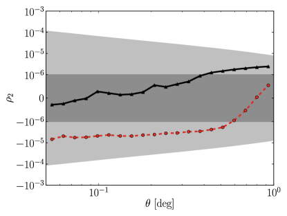
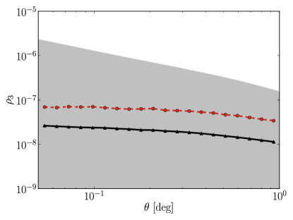
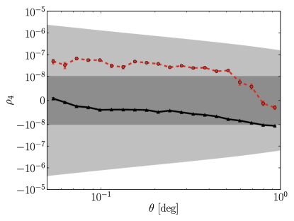
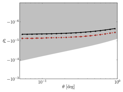
Finally, we need to place a requirement on how PSF model shape errors propagate into an additive term in the shear-shear correlations. The expression for these additive terms is found in equation (3.17) in Jarvis et al. (2016), and depends on the five $\rho$ statistics, two of which were defined in Rowe (2010) and the final three in Jarvis et al. (2016). If we define $\delta g_{\text{PSF}}^{*}\equiv g_{*}-g_{\text{PSF}}$, evaluating the PSF model at the positions of the stars, then the first two $\rho$ statistics are defined as

$$\rho_{1}(\theta) \equiv\left\langle\delta g_{\text{PSF}}^{*}(\vec{r})\delta g_{\text{PSF}}(\vec{r}+\vec{\theta})\right\rangle$$ (26)

$$\rho_{2}(\theta) \equiv\left\langle g_{\text{PSF}}^{*}(\vec{r})\delta g_{\text{PSF}}(\vec{r}+\vec{\theta})\right\rangle.$$ (27)

Conceptually, $\rho_{1}$ is the auto-correlation function of PSF model shape residuals, while $\rho_{2}$ is its cross-correlation with the PSF shape itself. The remaining $\rho$ statistics involve $T_{\text{psf}}$, the trace of the second moment matrix of the PSF. They are used to estimate the systematic uncertainty in the shear correlation function due to PSF modeling errors.

$$\rho_{3}(\theta) \equiv\left\langle\left(g_{\text{PSF}}^{*}\frac{\delta T_{\text{PSF}}}{T_{\text{PSF}}}\right)(\vec{r})\left(g_{\text{PSF}}\frac{\delta T_{\text{PSF}}}{T_{\text{PSF}}}\right)(\vec{r}+\vec{\theta})\right\rangle$$ (28)

$$\rho_{4}(\theta) \equiv\left\langle\delta g_{\text{PSF}}^{*}(\vec{r})\left(g_{\text{PSF}}\frac{\delta T_{\text{PSF}}}{T_{\text{PSF}}}\right)(\vec{r}+\vec{\theta})\right\rangle$$ (29)

$$\rho_{5}(\theta) \equiv\left\langle g_{\text{PSF}}^{*}(\vec{r})\left(g_{\text{PSF}}\frac{\delta T_{\text{PSF}}}{T_{\text{PSF}}}\right)(\vec{r}+\vec{\theta})\right\rangle$$ (30)

We define a maximum tolerable additive systematic on $\xi_{+}(\theta)$ due to PSF model shape errors, by requiring that each $\rho$ statistic contribute less than $0.5\delta\xi_{+,\text{sys}}$. In that case, our requirements on the $\rho$ statistics are

$$|\rho_{1,3,4}(\theta)|<\left\langle\frac{T_{\text{PSF}}}{T_{\text{gal}}}\right\rangle^{-2}\delta\xi_{+,\text{sys}}$$ (31)

and

$$|\rho_{2,5}(\theta)|<|a|^{-1}\left\langle\frac{T_{\text{PSF}}}{T_{\text{gal}}}\right\rangle^{-1}\delta\xi_{+,\text{sys}}$$ (32)

where $a$ and $\delta\xi_{+,\text{sys}}$ are defined as in Section 3.3.3. As in Section 3.3.2, we adopt a value of $\langle T_{\text{PSF}}/T_{\text{gal}}\rangle=1$ for setting requirements. The value of $|a|$ is estimated using simulations in Mandelbaum et al. (2017) as described in Section 6.2 in this paper; we calculate its lensing-weighted average as approximately 0.02. Finally, using the same (conservative) integrated SNR argument as in Section 3.3.2 to avoid a binning-dependence of the requirement, these requirements become

$$|\rho_{1,3,4}(\theta)|<\frac{\xi_{+}(\theta)}{2\,\text{SNR}_{\text{s-s}}}=\frac{\xi_{+}(\theta)}{25}$$ (33)

and

$$|\rho_{2,5}(\theta)|<\frac{\xi_{+}(\theta)}{2|a|\,\text{SNR}_{\text{s-s}}}=\frac{\xi_{+}(\theta)}{25|a|}.$$ (34)

3.4 Overall summary of requirements

In Table 1 we summarize the key requirements in this section. In the case of requirements on the same quantity provided by galaxy-galaxy lensing and cosmic shear, we have always adopted the more stringent requirement (from g-g lensing in our case).

Table 1: Summary of key requirements from Section 3.

Systematic uncertainty	Origin
Overall multiplicative bias	Galaxy-galaxy lensing, Section 3.2.1, equation (6)
Multiplicative bias due to PSF model size errors	Galaxy-galaxy lensing, Section 3.2.2, equation (10)
Overall additive bias correlation function	Cosmic shear, Section 3.3.3, equation (22)
Additive bias due to insufficient correction for PSF anisotropy	Cosmic shear, Section 3.3.3, equation (24)
PSF model shape errors	Cosmic shear, Section 3.3.4, equations (33) and (34)

Figure 4: $i$-band PSF magnitude distribution of the PSF star sample in each field.

4 PSF modeling tests

In this section, we describe tests of the fidelity of the PSF modeling. Bosch et al. (2017) show tests of PSF modeling on individual exposures, including plots of PSF model size and shape residuals as a function of focal plane position, while this paper focuses on tests of the coadd PSF, since that is the relevant quantity for shear estimation.

We begin with a definition of the star samples used for internal (to the data) tests of PSF models, and then describe the PSF model tests. Note that no external simulations were used for tests of PSF models. This is because the tests internal to the data that we will show below suggest that PSF modeling errors are not a limiting systematic for first-year HSC data. In future years, when statistical errors are reduced due to the larger data volume and other systematic errors are reduced through further study, PSF modeling will require more scrutiny, perhaps including external simulations.

The above statement about the impact of PSF modeling errors is valid only after some area cuts were placed on the fidelity of the PSF model size. Tests indicated that PSF models had serious problems in very good seeing ($<0.45$) as shown in more detail in Bosch et al. (2017).

To bypass this problem, we introduced two cuts, both of which were briefly mentioned in Section 2.2 but will be described in more detail here. The first cut removes visits in the VVDS field with PSFs which are too good to be modeled by PSFEx properly before these visits go into the coadding process. In most cases such visits have seeing better than $0.45^{\prime\prime}$ at the center of the field-of-view. This reduction is denoted as S16A.wide2, with details described in the HSC DR1 paper.

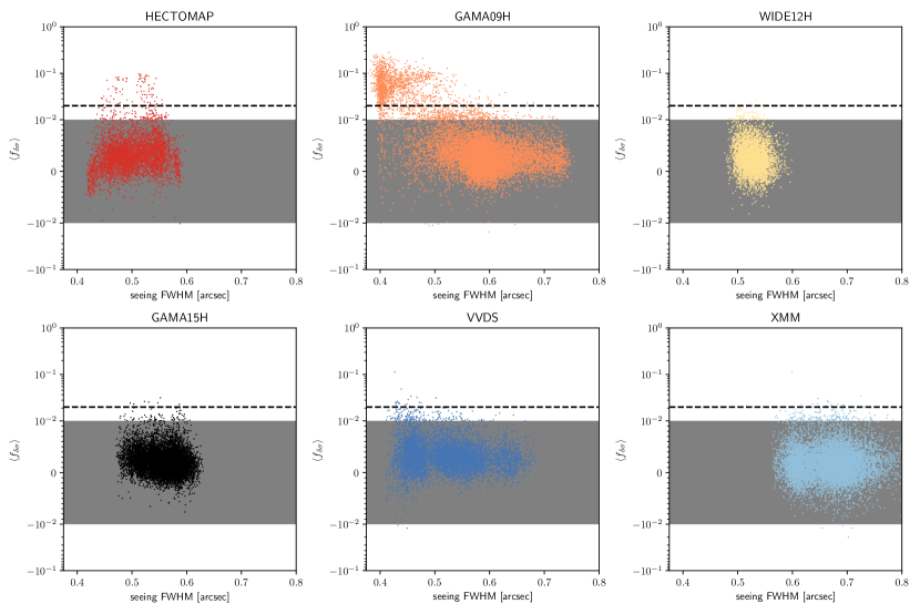
The second cut is to ensure that the PSF size is adequately modeled. For this purpose, we calculate the fractional size residual of PSF stars (defined as described in Section 2.3) which is defined by $f_{\delta\sigma}=(\sigma_{\rm PSF}-\sigma_{*})/\sigma_{*}$, where $\sigma_{*}$ and $\sigma_{\rm PSF}$ are the determinant radius of PSF stars and PSF models (from the adaptive second moments) reconstructed at the PSF star positions, respectively. To suppress measurement noise, we average the fractional size residuals $f_{\delta\sigma}$ within a HEALPix pixel with ${\tt NSIDE}=1024$, which corresponds to an area of $\sim 12\ {\rm arcmin}^{2}$. The number of PSF stars in a HEALPix pixel varies from $\sim 10$ to $\sim 24$. We then plot the fractional size residual $f_{\delta\sigma}$ as a function of seeing FWHM (also based on the average size of PSF stars averaged within HEALPix pixels), as shown in figure 5. In the GAMA09H field, we find a cloud of HEALPix pixels with very good seeing ($\sim 0.45^{\prime\prime}$) and large fractional size residual ($f_{\delta\sigma}\sim 0.02$–0.2, with strictly positive values indicating a systematic bias). We find that the inclusion of these regions degrades several of our PSF model-related null tests for the GAMA09H field, so that it fails the requirements quite severely. After we remove such areas by applying the $f_{\delta\sigma}<0.02$ cut, which removes $\sim 4$% of the total WLFDFC area (primarily in GAMA09H but affecting HECTOMAP slightly, as well), $\rho_{1}$ goes down and meets the requirement.

This two-step approach was necessary because the first cut was intended to eliminate the problem as originally noticed in VVDS, but later there were areas that were found to fail our requirements in GAMA09H, necessitating a second cut that could be applied in postprocessing.

All tests described below use the final area of the shear catalog, after imposing these cuts on PSF model quality.

Figure 5: The average fractional size residual $\langle f_{\delta\sigma}\rangle=\langle(\sigma_{\rm PSF}-\sigma_{*})/\sigma_{*}\rangle$ between PSF stars and PSF models reconstructed at star positions, averaged over the PSF stars within HEALPix pixels with ${\tt NSIDE}=1024$, and shown for each HEALPix pixel as a function of seeing. A symlog scale is used to allow negative residuals to be shown. The dashed line shows the fractional size cut we apply, removing all points above the line and therefore eliminating the cloud of points with large strictly positive $\langle f_{\delta\sigma}\rangle$ values that often but not always have very good seeing. The best-seeing visits in the VVDS region were already removed before production of this figure. Regions with a dark grey background show the linear part of the symlog scale, with the rest being logarithmic.

4.1 Star samples used

As described in more detail in Section 2.3, PSF star selection relies on clustering of high-SNR objects in size, typically resulting in $\sim 90$ star candidates per CCD chip. Currently, $\sim$20$\%$ of the stars in a given exposure are randomly chosen and reserved for cross-validation and are not used for PSF modeling. We found that the quality of the modeling was almost independent of the number of stars as long as there were at least 20 stars used. This was true for $\sim 99\%$ of the individual visists. Therefore, reserving 20$\%$ of the stars did not degrade the quality of the PSF models.

We define two star samples for PSF modeling tests. The first includes stars used for the PSF determination by PSFEx and the other includes bright, secure star detections that were not used for PSF. Because the star sample used in PSFEx is derived on individual exposures, different exposures will not necessarily select the same set of stars. We label stars that were used on $\geq 20\%$ of the input visits as having been used in the modeling; because most of the Wide survey has six exposures in $i$, this typically requires a star to be selected for PSF determination in at least two exposures.

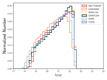
The other set of stars we define are secure star detections that were not used for PSF determination, but that were otherwise selected with the same flag and other cuts. The latter are important to use for testing in case over-fitting results in an overly optimistic result on our null tests using PSF stars, and/or to pick up on PSF interpolation failures. For both catalogs, we first remove objects whose photometry might be suspected due to a contamination at the edges of CCDs and pixels with saturation, interpolation, and cosmic rays, and with bad centroid and shape measurement flags. We then select stars by iclassification_extendedness=0 (a star/galaxy classifier based on the $i$-band images; Bosch et al. 2017) and restrict to a bright sample using $i$-band PSF magnitude $<22.5$. As shown in figure 4, this is quite close to the effective magnitude limit of PSF stars. This choice is motivated by the finding (figure 13 of the HSC DR1 paper) that the star sample in this magnitude range is highly pure, but contamination by galaxies becomes more important at fainter magnitudes.

The PSF star sample is flagged by setting icalib_psf_used=True. Figure 4 shows the distribution of $i$-band PSF magnitudes of this sample for different fields. The magnitude of PSF stars ranges from $i_{\rm PSF}\sim 18$ to $22.5$.

4.2 Internal tests

For weak lensing, we need to validate both the PSF model sizes and shapes. Errors in the former result in multiplicative biases in shear estimates, while errors in the latter result in additive biases in shears. For our tests, we use the effective stacked PSF (see Section 2.3 for details), and compare with measurements of the stars in the coadd. Bosch et al. (2017) shows the result of PSF model tests on individual visits. As described in Section 4.1, we carry out the majority of our tests separately with two secure star samples: those that were and were not used to construct the PSF models.

Figure 6: Top left: Distribution of the fractional size residual of the PSF star sample in each field. The size is defined by the determinant radius. The gray shaded regions indicate the requirements on the mean residual for the first-year HSC survey data. The vertical dashed lines show the median of the fractional size residual of each field; the results are highly consistent across fields. Top right: Same as the top left, but for non-PSF stars, reweighted in order to match the SNR distribution of the PSF stars used to make the top left panel. Bottom left: Solid lines are median and bootstrap error of residual size of the PSF stars after brighter-fatter correction, as a function of the $i$-band PSF magnitude. Dashed lines are without brighter-fatter correction, as calculated using the first 61.5 nights of data through November 2015 (hence the observed area is different from what went into the solid lines). The gray shaded regions indicates the requirements on the mean residual for the first-year HSC survey data. Bottom right: The correlation function of the fractional size residuals as a function of separation $\theta$. Solid and dashed lines show results for PSF and non-PSF stars, respectively.

4.2.1 PSF model size

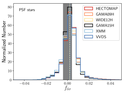
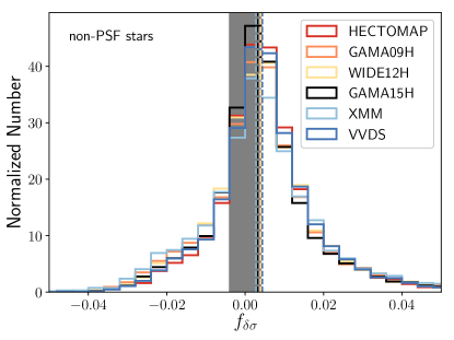
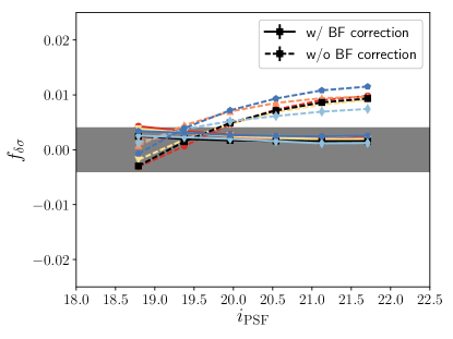
The results for all PSF model size tests are shown in figure 6. For the size, we use the determinant radius $\sigma$ for the star images and the PSF model, based on the adaptive second moments, to calculate the fractional size residual $f_{\delta\sigma}=(\sigma_{\rm PSF}-\sigma_{*})/\sigma_{*}$.

As shown in the top left panel of figure 6, the distribution of fractional PSF size residuals is narrowly peaked at 0 for all fields. Nearly all stars used for this test (PSF stars only) fall within the shaded region defined by our first year requirements. The median values shown as vertical dashed lines fall within the first year requirements region. The top right panel shows the same thing, but for non-PSF stars. To make this plot, we have reweighted the stars to ensure that their SNR distribution matches that for PSF stars, to ensure that different levels of noise in the $\sigma_{*}$ estimates does not change the width of the distribution. Here the scatter is clearly larger; the median values are close to the edge of our requirements, but still pass. Given the conservative assumptions made in defining the requirements, this is acceptable performance. However, for the full survey, we may need an improved PSF modeling algorithm to achieve the more stringent resulting requirements. Note that with this histogram alone, we cannot distinguish whether the additional width indicates overfitting in the PSF modeling process, or use of an insufficient PSF model interpolation scheme. In Bosch et al. (2017), a similar test carried out with the single-epoch images that are used directly for PSF modeling produced results that are qualitatively similar to what we see here in the coadd.

It does not seem obvious that the distribution of the quantity shown in figure 6 is the same as the quantity shown on the horizontal axis of figure 5. The primary reason for this is that figure 6 shows the results for individual stars, which is substantially noisier than the results averaged within HEALPix pixels shown in figure 5. For the earlier plot, our goal was to identify outlier regions, so we had to average over stars to reduce the noise that dominates the shape of the per-star histograms in the later plot. A much more minor contributor to the differences between figures is that the quantity plotted has a different denominator in each case. For the earlier plot, we used $\sigma_{*}$ because $\sigma_{\text{PSF}}$ has significant errors in the outlier regions we had hoped to identify. For the later plot, we used $\sigma_{\text{PSF}}$ to reduce noise.

The lower left panel is a comparison of the average fractional size residual in bins of fixed $i$-band PSF magnitude for two versions of the HSC pipeline: an older version without correction for the brighter-fatter effect, and the version used for science including a brighter-fatter correction. As shown, the version of the pipeline (dashed curves) without this correction shows the characteristic signature of this systematic error: stars appear larger than the PSF model at the brightest magnitudes, and smaller than the PSF model at fainter magnitudes. This trend is almost completely removed by the brighter-fatter correction, giving PSF size residual curves that are almost independent of magnitude. The brighter-fatter correction is necessary to ensure that we meet our requirements for first-year weak lensing science. This test again uses only the PSF star sample, however the efficacy of the brighter-fatter correction should be the same for all stars at fixed magnitude, so we do not expect results to differ for the non-PSF star sample (which has the same magnitude range).

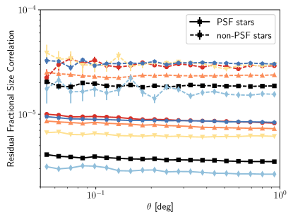
Finally, the bottom right panel of figure 6 shows the spatial correlation function of the PSF fractional size residuals. Note that curves are shown separately for PSF stars (solid) and non-PSF stars (dashed). All of these curves are nearly independent of spatial separation and differ from field to field, unlike the distribution of fractional size residuals, which are consistent across fields. We can also see that the fields with the best seeing, VVDS and HECTOMAP (see figure 1), have the worst PSF model size residual correlation functions. Finally, comparing the PSF stars and non-PSF stars, we can see that the latter have a larger value of this correlation function, again flat with scale. The field-to-field trends are similar to what we saw for the PSF stars. This increase in the correlation function as we move from PSF stars to non-PSF stars is suggestive of either problems with the PSF model interpolation or overfitting. However, the plot does not provide us with information to distinguish between these options.

The important result of this section, however, is that while our PSF model size diagnostic for non-PSF stars (which are likely more representative of PSF model fidelity at galaxy positions) is worse than when we use PSF stars, the results are still within our first-year HSC science requirements.

One notable aspect of these results is the fact that $\langle\sigma_{*}-\sigma_{\text{PSF}}\rangle<0$, that is, on average the stars on the coadd are slightly smaller than the stacked PSF model at the 0.1% level. In general, we expect that the impact of relative astrometric errors will be to make the stars on the coadd appear slightly broader than the stacked PSF model. Given the sign of the average PSF size residual, we infer that the impact of relative astrometric errors cannot be responsible for this difference.

Figure 7: Distributions of PSF residual shape of the non-PSF star sample in each field.

Figure 8: PSF residual shape correlations, or $\rho$ statistics, $\rho_{1}$ through $\rho_{5}$ (defined in Section 4.2.2) as a function of separation $\theta$ on the sky. The top left panel shows $\rho_{1}$ for each field to illustrate the significant field-to-field differences. The color scheme for the fields is the same as in figure 7 (with an additional black curve showing the field-averaged results), while solid and dashed lines show results for PSF and non-PSF stars, respectively. The remaining panels show the $\rho$ statistics averaged over the whole shape catalogue area along with our science requirements for first-year survey science as determined in Section 3.3.4. Here too the solid and dashed lines show results for PSF and non-PSF stars, respectively. Since the $\rho$ statistics can be negative, the vertical axes use a symlog scale. Regions with a dark grey background show the linear part of the symlog scale, with the rest being logarithmic. Regions with a light grey background are within the first-year survey requirements for cosmic shear.

4.2.2 PSF model shape

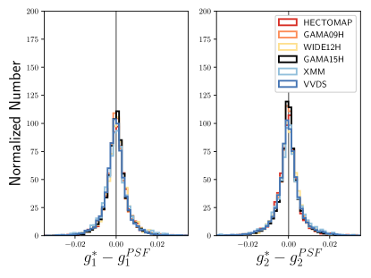
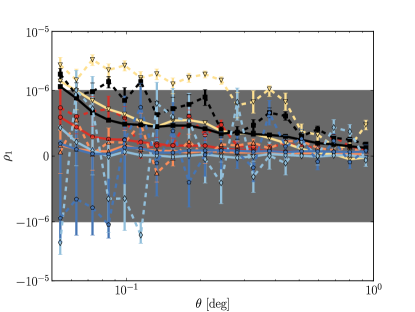
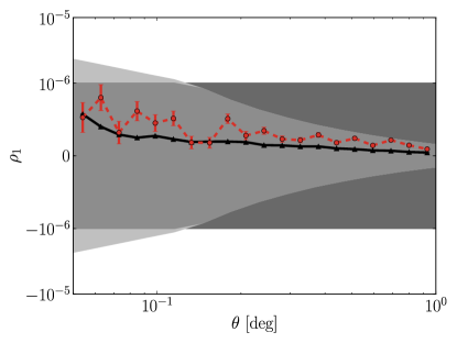
The results for all PSF model shape tests are shown in figure 7 and 8. While the shape definition returned by our shape measurement algorithms is the distortion defined in equation (2), we divide by two to obtain shear estimates (this conversion is correct for stars and PSFs).

Figure 7 shows the distribution of star $-$ PSF shears for the PSF star sample in each field. The typical width of the distributions is $<0.01$, with the means quite close to zero.

The panels in figure 8 show the $\rho$ statistics, defined in this paper in equations (26)–(30) based on previous work (Rowe, 2010; Jarvis et al., 2016). These statistics are constructed from spatial correlation functions of PSF model shape and size residuals. Requirements on the $\rho$ statistics were discussed in Section 3.3.4.

On all $\rho$ statistics, we show results for PSF stars (solid lines) and non-PSF stars (dashed lines). Clearly the results are not consistent in the two cases. As shown in the top left panel of figure 8, there is clearly field-to-field variation in $\rho_{1}$; the same is true for the other $\rho$ statistics.

The remaining panels of figure 8 show the survey-averaged $\rho$ statistics compared with first-year survey requirements. The results are consistently worse for the non-PSF stars than for PSF stars, possibly due to inaccurate PSF interpolation or over-fitting; however, the results are within our (relatively conservative) first-year requirements in all cases. The discrepancy between results with PSF stars and non-PSF stars is particularly striking for $\rho_{2}$ and $\rho_{4}$. These are the only two of the $\rho$ statistics that incorporate a PSF model shape correlated against a PSF model shape error.

We have the least margin on $\rho_{1}$, which when measured with non-PSF stars, is close to our requirements envelope for $\theta>0.3^{\circ}$. This finding, combined with the mean PSF model size residual in the previous subsection, suggests that an improved PSF modeling algorithm may be needed to achieve our weak lensing science goals with the full HSC survey area.

5 Shear catalog

In this section, we describe the shear catalog, including the galaxy selection criteria (Section 5.1), its basic properties (Section 5.2) and null tests (Section 5.3). We refer the interested reader to Appendix A for more details on the quantities provided in the catalogs.

5.1 Galaxy selection

In this subsection, we discuss the galaxy selection criteria that are imposed after all area cuts summarized in Section 2.2. We describe these cuts and their purpose qualitatively, while in Appendix B, we give the exact flags and database columns to enable reproducibility. Users who apply their own cuts that are less stringent than the ones given here should be aware that the validation tests in this catalog were not performed for galaxies that failed the cuts given below.

We begin with a set of cuts on HSC pipeline flags, where all of the below cuts are imposed in the $i$ band and most of these are explained further in the HSC DR1 paper. First, we required that idetect$\_$is$\_$primary be set; this flag is used to identify a single version of each astrophysical object, by rejecting duplicates due to overlap between different patches or tracts as well as still-blended parent objects (whose children are also measured). We also imposed cuts to avoid objects with problematic image processing, including the following scenarios: extremely large groups of objects that the deblender skipped (usually caused by bright stars); those with a failure in the centroiding algorithm; those too close to an image boundary; those with a pixel very close to the object center that was flagged as interpolated, saturated, a cosmic ray hit, otherwise bad, or just short of saturation (where nonlinearity corrections are less certain); and those for which the shape measurement algorithm returned an error code or a value of NaN for the shape measurement uncertainty. Finally, we required that the object have been classified as extended (not a point source) by the HSC pipeline.

In addition to flag cuts, we impose the following cuts on $i$-band object properties:

• The unforced cmodel $i$-band magnitude should be below $24.5$ after extinction correction. There are two reasons for this conservative cut. First, our spectroscopic training sample used to calibrate photometric redshifts has very few objects fainter than this, which results in significant systematic uncertainty in the photo-$z$ calibration. Second, the simulations that we use to calibrate our shear estimates are based on the HST COSMOS survey, with galaxies with parametric model fits limited to $I<25.2$. Given that the inserted galaxies have some scatter in their observed magnitudes, $24.5$ seems to be the practical limit before we start running out of galaxies due to the limitations of our parent sample. In future years of HSC survey analysis, we hope to relax this cut and take a more full advantage of the depth of HSC data for our lensing shear catalogs.

• The unforced cmodel $S/N$ should be $\geq 10$. Note that given the magnitude cut above, this cut is not very important in practice, as the $S/N$ distribution drops sharply below $S/N=$20.

• Resolution factor (equation 4) $R_{2}\geq 0.3$. A completely unresolved object will have $R_{2}=0$, while a fully resolved one will have $R_{2}=1$.

• Total magnitude of the distortion (after PSF correction) defined in equation (2) should satisfy $|e|<2$. Due to noise, the distribution of distortion values extends into the non-physical $|e|>1$ regime. Truncating the distribution too aggressively at $1$ leads to a negative shear bias; however, some truncation is needed to enable mean shear statistics to converge.

• The catalog estimate of the shape measurement uncertainty due to pixel noise, $\sigma_{e}$, should lie in the range $[0,0.4]$. This cut removes only a tiny fraction of highly anomalous objects, $<1$% of those that pass the other cuts.

• Multi-band detection cut, defined by requiring at least two other bands (out of $grzy$) to have a cmodel detection significance exceeding 5. This cut removes a very small fraction of objects, $<1$%, that pass our other cuts. In addition to ensuring enough color information to compute a photometric redshift, this cut also helps remove junk detections, asteroids (Hildebrandt et al., 2017), and so on.

• The blendedness parameter, iblendedness$\_$abs$\_$flux, which quantifies the relative contamination of the object light profile by the light from other nearby objects, should be less than $10^{-0.375}$. As defined in section 4.9.11 in Bosch et al. (2017), the blendedness parameter would have a value of 0 for isolated objects by definition, while objects detected as being strongly blended would have a blendedness value approaching 1. The cut value was determined in two stages. First, an examination of the distribution of $R_{2}$ values in narrow bins in $\log_{10}{b}$ showed that above this value, the distribution of $R_{2}$ was skewed in an unphysical way towards very high resolution factor even for quite faint objects. Second, visual inspection of the objects above that cut value revealed that they preferentially lie very near bright galaxies, and were either spurious detections or real detections of objects with completely unreliable photometry and shape measurement due to contamination by light from the nearby bright galaxy (Murata et al., in prep.). This cut value removes of order 1% of the objects that would pass the other cuts, and should be considered a method of junk removal; it does not constitute an attempt to remove mildly blended objects from the catalog. While a bug in the blendedness calculation was identified after introduction of this cut, as noted in Bosch et al. (2017) and quantified in Murata et al. (in prep.), the bug resulted in a very small remapping of the blendedness values that does not cause significant problems for our use of this cut value.

• As noted in Section 2.3.3, the object must lie in a region where all overlapping exposures contributed to the coadd, so the coadded PSF model (which does not account for missing pixels within sensors) is correct. Due to a bug in hscPipe, this filtering was not complete; a small number of objects lying on CCD boundaries, sensor defects, or cosmic rays were not flagged by the pipeline and could not be removed in this cut. The internal PSF quality tests in Section 4.2 are sensitive to this problem, however, and demonstrate that its effects do not cause the PSF model errors to exceed our requirements.

For the sake of scientific reproducibility, the publicly released shear catalog has a flag indicating whether all lensing cuts are passed by each object. Users do not have to separately try to impose all flags and cuts on galaxy properties.

Figure 9: The effective (weighted) galaxy number density as a function of seeing in each field. Green points are the density as computed on a regular grid with spacing of 0.5 arcmin on the tangent-projected sky using Gaussian smoothing with $\sigma\sim 1.06$ arcmin. The red curves on each panel are the mean number density as a function of seeing in each field, while the black points with errorbars show the mean and standard deviation at fixed FWHM across the entire survey.

Figure 10: Unweighted (raw) number density of sources passing all lensing cuts in each field.

Figure 11: Weighted number density of sources passing all lensing cuts in each field.

Figure 12: Top left, top right, bottom left, and bottom right panels show the lensing-weighted distributions of galaxy $R_{2}$ values, $i$-band cmodel $S/N$, $i$-band cmodel magnitude, and total distortion magnitude $|e|$ for each survey region after all selection criteria were imposed. The $|e|$ distribution extends into the unphysical $|e|>1$ regime because $e$ is defined by taking the ratio of two noisy quantities, and thus noise fluctuations can create an unphysical tail.

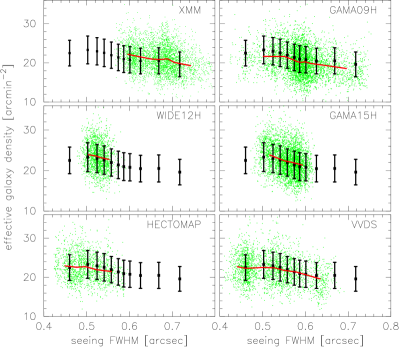
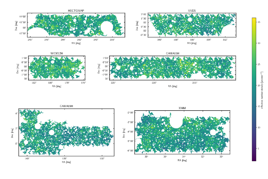
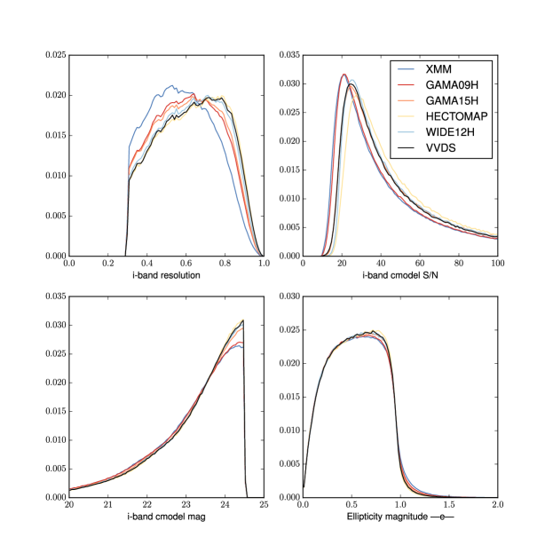
With $>12$ million galaxies in the catalog after these cuts, and an area of 136.9 deg², the average source galaxy number density without any lensing weights is 24.6 arcmin^-2. Inclusion of lensing weights (described in Section 5.2) gives $n_{\text{eff}}=21.8$ arcmin^-2. Cuts on photo-$z$ quality or photo-$z$ values will reduce this number further, but the level of reduction depends on the photo-$z$ algorithm.

5.2 Basic characterization

Here we present the basic characterization of the galaxy properties in the shape catalog.

Figure 13: Stacked tangential (upper) and cross (lower) shear profiles around random points, averaged across the entire survey. The number density of the random points is 50 deg^-2. Errors are estimated from mock catalogs which follow the same spatial distribution of galaxies as the HSC shear catalog and includes cosmic shear from ray-tracing simulations (see Oguri et al. 2017 for more details). The $\chi^{2}$ and $p$-value for the null hypothesis for each field are summarized in Table 2.

Figures 10 and 11 show the unweighted and weighted (respectively) galaxy number densities after all selection criteria from Section 5.1 are imposed on the sample. Here, the weight is the inverse variance weight based on the quadrature sum of shape noise and measurement error,

$$w=\frac{1}{\sigma_{\text{SN}}^{2}+\sigma_{e}^{2}}.$$ (35)

Both quantities in this weight were estimated using simulations, see Section 6. Note that the weighted and unweighted number densities differ by only $\sim 12$% because the shape catalog does not go to very low $S/N$ detections. The trend in number density as a function of seeing is shown in figure 9 separately for each field.

Finally, figure 12 shows the lensing-weighted distributions of several galaxy properties in each survey field separately. As shown, the distributions of resolution factor $R_{2}$ vary noticeably, in a way that is consistent with per-field trends in seeing (figure 1). For example, the fields with the best (worst) seeing have the highest (lowest) resolution factors. There are similar trends for $S/N$, except that VVDS has only typical $S/N$ despite having nearly the best seeing because of the omission of some exposures (figure 2). However, the magnitude and distortion distributions are similar across all fields.

Table 2: $\chi^{2}$ values and $p$-values for testing whether stacked $+$ and $\times$ shear profiles around random points (like figure 13 but also showing numbers separately for each field), $+$ and $\times$ shear profiles around bright stars in figure 14, and $\times$ shear profiles around CMASS galaxies in figure 15, are consistent with zero signal. The last row shows $\chi^{2}$ values and $p$-values for all fields combined. The $\chi^{2}$ values for the first two columns have 15 degrees of freedom, while those for the last three columns have 20 degrees of freedom.

Field	Random $g_{+}$	Random $g_{\times}$	Bright star $g_{+}$	Bright star $g_{\times}$	CMASS $g_{\times}$
	$\chi^{2}$ ($p$-value)	$\chi^{2}$ ($p$-value)	$\chi^{2}$ ($p$-value)	$\chi^{2}$ ($p$-value)	$\chi^{2}$ ($p$-value)
GAMA09	22.80 (0.09)	15.11 (0.44)	32.24 (0.04)	22.73 (0.30)	27.17 (0.13)
GAMA15	14.34 (0.50)	7.30 (0.95)	21.41 (0.37)	11.25 (0.94)	49.81 (0.00)
HECTOMAP	15.95 (0.39)	15.41 (0.42)	28.39 (0.10)	17.91 (0.59)	18.69 (0.54)
VVDS	24.25 (0.06)	14.99 (0.45)	14.32 (0.81)	30.94 (0.06)	12.58 (0.90)
WIDE12H	29.24 (0.02)	15.61 (0.41)	23.29 (0.28)	16.21 (0.70)	14.94 (0.78)
XMM	9.79 (0.83)	11.09 (0.75)	25.08 (0.20)	27.15 (0.13)	17.54 (0.62)
All fields combined	20.04 (0.17)	11.65 (0.71)	28.04 (0.11)	27.35 (0.13)	27.66 (0.12)

Figure 14: Average tangential and $\times$ shear around bright stars across the entire survey, defined as all stars with $i$-band magnitude $\leq 22.5$ (and passing other cuts as defined in Section 4.1). We restrict ourselves to small scales here so that we can investigate the impact of nearby stars on shear estimates, for example due to their inducing errors in sky background estimation.

Figure 15: Average cross shear around SDSS CMASS galaxies across the entire survey at all redshifts. This quantity should be zero due to symmetry.

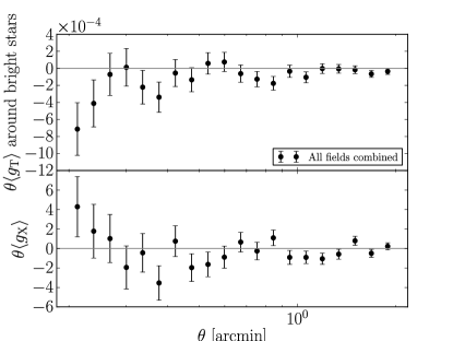
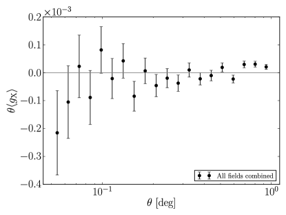
5.3 Null tests

In this section, we present a set of null tests for the galaxy shape catalog. Note that all null tests include statistical corrections for additive and multiplicative biases following a formalism similar to Appendix C.

As a first test, we calculate the mean shear estimates $\langle g_{1}\rangle$ and $\langle g_{2}\rangle$ within each of the six survey fields in sky coordinates, which are quite close to CCD coordinates for most of our fields. To ascertain the significance of any non-zero values, we must estimate errorbars including not only shape noise but also cosmic shear using many realizations of mock shear catalogs based on $N$-body simulations with the same area coverage as the HSC survey. Of the twelve numbers calculated (weighted mean values of two shear components in six fields), we compute the $p$-value for a fit to zero signal. Only one of the twelve $p$-values is below a nominal threshold of 0.05, and that one is still quite marginal ($p=0.03$), giving no reason to suspect a systematic from this test.

Figures 13 and 14 show the stacked $+$ and $\times$ shear signals as a function of angular separation from random points and bright stars, respectively. The first of these goes to scales of 100 arcmin, to investigate large-scale systematic shear (which is revealed as the angular scales get large enough that some of the annuli around the random points are incomplete). The second is on small scales only, and the goal in this case is to test for possible apparent tangential or radial shears due to sky background misestimation near bright objects. Finally, figure 15 shows the $\times$ shear component around BOSS CMASS galaxies out to large scales. As shown, there is no evidence for any statistically significant detection for any of our survey fields, over any range of scales. The $\chi^{2}$ and $p$-values for a fit to zero signal are shown in Table 2.

Figure 16: Average $g_{1}$ values as a function of various parameters; $i$-band cmodel $S/N$ (upper left), $i$-band cmodel magnitude (upper right), the resolution factor, (lower left), and PSF FWHM (lower right). Here $g_{1}$ is defined in the sky coordinates, which are very close to CCD coordinates for most of our fields. As in figure 13, errorbars are from mock shear catalogs and therefore include cosmic shear.

Figure 17: Star-star (left) and star-galaxy (right) shear correlation functions $\xi_{+}$. Solid and dashed lines were calculated using PSF and non-PSF stars, respectively. Error bars are shown, but are generally smaller than the size of the plotted points. For this plot, we have only shown $\xi_{+}$ because it carries nearly all the useful information. However, we note that $\xi_{-}$ is consistent with zero for all fields on the scales on which we have shown $\xi_{+}$, except for HECTOMAP and VVDS. HECTOMAP has a slight negative $\xi_{-}$ at scales $>0.7^{\circ}$: $\leq 10^{-5}$ for the star-galaxy correlation and $\leq 10^{-4}$ for the star-star correlation, well below the $\xi_{+}$ measurement. VVDS has a slight negative $\xi_{-}$ of $\leq 10^{-5}$ in the star-star correlation only at scales $>0.7^{\circ}$.

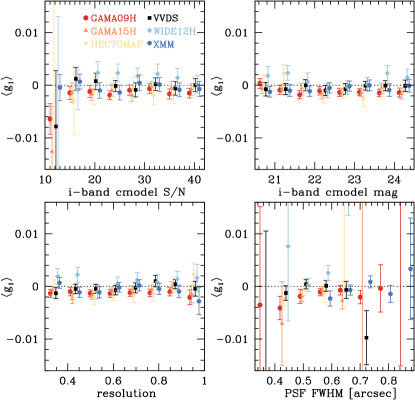
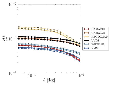
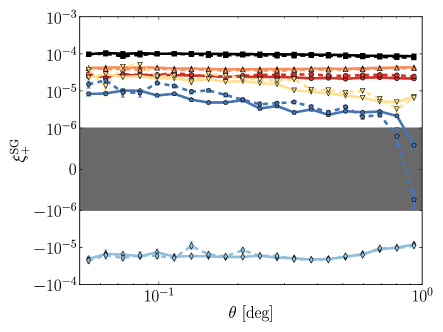
Figure 16 shows $\langle g_{1}\rangle$ in sky coordinates as a function of four properties of the $i$-band images: cmodel $S/N$ and magnitude, galaxy size, and PSF FWHM. Note that for most of our observations, sky coordinates are very close to CCD coordinates, so this plot has the potential to reveal systematics that correlate with the pixel directions. Results are similar for the other shear component (not shown). We find that the average shear values are consistent with zero, and the average shear values do not show any strong dependence on galaxy properties explored here. In some fields (e.g., GAMA09H and HECTOMAP), average shear values are persistently positive or negative in almost all bins. This is most likely due to the cosmic variance (cosmic shear) which produces correlated residuals between different bins of the galaxy properties. Bin-to-bin correlation coefficients range from 0.3–0.6. Other possible explanations for a nonzero mean shear signal, such as selection bias or incomplete correction for PSF anisotropy, would typically result in some dependence on galaxy properties – inconsistent with what is shown in this plot.

As an indication of PSF anisotropy leakage into galaxy shapes (combined with PSF shape modeling errors giving additive errors), figure 17 shows the star-star and star-galaxy shape correlation functions in each survey field, as measured using the PSF and non-PSF stars. In both panels, the star shapes are used directly without correction for the PSF, because the goal is to ascertain what fraction of the original PSF shape (as traced by star shapes) leaks into the galaxy shapes. First we consider the left-hand panel, the star-star correlations, where only $\xi_{+}$ (Eq. 11) is shown. These curves are fairly flat over separations of a degree, indicating that the PSF shape exhibits slow spatial variations in the coadd. The magnitude of the curves, from $2\times 10^{-3}$ for HECTOMAP down to $5\times 10^{-4}$ for XMM, reflects the typical PSF shape magnitudes from 0.05 down to 0.02 in these fields. The inverse correlation between seeing size and typical PSF shape may be caused by either increased contributions from optical distortions (Miyazaki et al., in prep.) in the very best seeing, or the fact that the amplitude of the atmospheric PSF ellipticity itself is inversely proportional to PSF size (Hamana et al., 2013).

One possible cause for a residual correlation between the shapes of stars and the PSF-corrected galaxy shapes is use of an insufficient PSF correction method. In the simplest case, where the measured ensemble shear is a linear combination of the true shear and the PSF shape due to residual PSF anisotropy in the galaxy shapes, $\langle\hat{g}_{\rm gal}\rangle=(1+m)\langle g\rangle+\langle ag_{\rm PSF}\rangle$, we should find a star-galaxy correlation that looks like

$$\langle g_{*}\hat{g}_{\rm gal}\rangle=(1+m)\langle g_{*}g_{\rm true}\rangle+a\langle g_{*}g_{\rm PSF}\rangle\sim a\langle g_{*}g_{*}\rangle,$$ (36)

meaning that the star-galaxy correlation function should be simply a rescaled version of the star-star correlation function with the same scale-dependence. Examining the correlation functions presented in figure 17, however, we see that this simple rescaling does not hold. Moreover, the relationship between the amplitudes of the star-star and star-galaxy correlations changes from field to field (not only in magnitude, but also in sign). We therefore conclude that the prescription in equation (36) must be an incomplete description of the star-galaxy correlations, with some other systematic error contributing. One candidate is a contribution from PSF modeling errors, which would give another term proportional to $\rho_{2}$ (shown in figure 8).

Next, we carry out an empirical test for the possible impact of either PSF ellipticity modeling errors or residual PSF anisotropy in galaxy shapes on cosmic shear two-point correlation function measurements. In the same prescription as equation (36), a residual correlation caused by PSF anisotropy leakage can be modeled by $\Delta\langle gg\rangle\sim a^{2}\langle g_{\ast}g_{\ast}\rangle$, and can be evaluated by the combination of

$$\xi_{\rm sys}\equiv\frac{\langle g_{*}\hat{g}_{\rm gal}\rangle^{2}}{\langle g_{*}g_{*}\rangle}.$$ (37)

PSF ellipticity modeling errors would also contribute additive terms, as discussed in Sec. 3.3.4. This null test therefore detects both types of systematic errors combined. Figure 18 shows $\xi_{\rm sys}$ for each field along with the standard $\Lambda$CDM prediction of $\xi_{+}$, the galaxy shear correlation function. The amplitude of $\xi_{\rm sys}$ varies among fields as expected from the above findings, and can be comparable to $\xi_{\rm gg}$ on degree scales, suggesting that marginalization over a template for $\xi_{\rm sys}$ may be needed on those scales. As was shown above, the amplitude of PSF anisotropy leakage may depend weakly on galaxy properties (primarily resolution factor), suggesting that an appropriate galaxy selection may reduce the amplitude of $\xi_{\rm sys}$. However, selection bias itself can cause some nonzero $\xi_{\rm sys}$, as can PSF modeling errors (illustrated through our small but non-zero $\rho$ statistics). Having identified this as a systematic that is likely to be important on the scales we would like to use for our analysis, we defer the detailed exploration of how to model this effect to reduce its impact on cosmological lensing analysis to future work. However, note that standard template marginalization schemes are a promising candidate for mitigation of this effect, given that its scaling with $\theta$ differs strongly from the scaling of cosmological lensing signals with $\theta$.

Figure 18: Separate panels show (for each survey field) the shape-shape correlation function $\xi_{+}(\theta)$ for PSF star shapes as points with errorbars; the predicted cosmic shear correlation function with a WMAP9 cosmology using the $n(z)$ from HSC photometric redshifts without any correction for photo-$z$ errors (which illustrates the approximate magnitude of the expected cosmic shear signal) as dashed lines; and $\xi_{\text{sys}}$, defined as $\xi_{\text{sg}}^{2}/\xi_{\text{ss}}$, as crosses.

Figure 19: Moments of B-mode mass map PDFs as a function of smoothing scale $\theta_{s}$. Mass maps are created using the standard Kaiser & Squires (1993) inversion technique (see Oguri et al. 2017 for more details). We show second (upper left), third (upper right), and fourth (lower left) moments, which are “de-noised” by subtracting moments originating from the shot noise (see, e.g., Van Waerbeke et al. 2013). Since the boundary of the survey region also induces some B-mode in mass maps, we subtract the average moments from the mock catalogs from the observed moments to correct for the boundary effect (see text for more details). Errors are also estimated from the mock catalogs. In the absence of systematic errors, these quantities should all be consistent with zero.

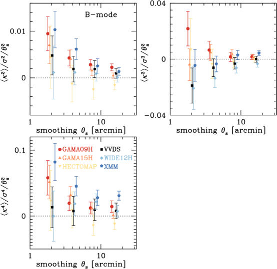
We can convert an observed shear field to a projected mass density (convergence) field because both are second derivatives of the gravitational potential (Kaiser & Squires, 1993). Weak gravitational lensing produces mostly “E-mode” convergence fields, whereas many potential systematic effects produce both “E-mode” and “B-mode” convergence fields. As a result, B-mode convergence fields (mass maps), which are produced by curl-like patterns in the shear field, are used to check for the presence of certain residual systematics in weak lensing shear catalogs (e.g., Massey et al., 2010). While not all systematics will produce a B-mode signature, this is nonetheless an important null test. Here we present some results of our mass map analysis. Additional mass map analysis and further details about the mass map production is presented in Oguri et al. (2017).

Figure 19 shows the second, third, and fourth moments of the B-mode mass map probability distribution function (PDFs) as a function of smoothing scale, separately for each survey field. These moments are “de-noised” by subtracting moments originating from the shot noise (see, e.g., Van Waerbeke et al. 2013), and should therefore be consistent with zero in the absence of systematics. It is known that boundary and masking effects also produce non-zero moments in the B-mode mass map PDFs, even after subtracting the shot noise contribution. We account for these effects using mock shear catalogs (Oguri et al., 2017). The mock shear catalogs have the same spatial distribution of galaxies as the HSC shear catalog, but their ellipticity values are replaced with simulated values that include the intrinsic ellipticity and cosmic shear from ray-tracing simulations (Shirasaki et al., 2017; Takahashi et al., 2017). Since the mock shear catalogs have the same masking pattern and spatial inhomogeneity as the HSC shear catalog, we remove the boundary and masking effects by subtracting the average moment values computed using the mock shear catalogs from those computed using the real HSC shear catalog. As shown in this figure, the moments after the correction for the boundary and masking effects are mostly consistent with zero within $\sim 2\sigma$ level. This means that the B-mode mass map PDFs are sufficiently close to Gaussian, as expected in the case of no systematic effects. Small deviations from zero must originate from PSF leakage as examined above, or PSF modeling errors as we will discuss below.

Mass maps can also provide a complementary check of the PSF leakage and PSF modeling errors. Figure 20 provides an alternative view of star-galaxy cross correlations. We cross-correlated mass maps and “star mass maps” which are mass maps constructed using star ellipticities (for more detail, see Oguri et al., 2017). We then quantify the correlation of two maps, $\kappa_{1}(\boldsymbol{\theta}_{i})$ and $\kappa_{2}(\boldsymbol{\theta}_{i})$ (which are normalized to zero mean, i.e., $\langle\kappa_{1}\rangle=\langle\kappa_{2}\rangle=0$), using the Pearson correlation coefficient $\rho_{\kappa_{1}\kappa_{2}}$ defined as

$$\rho_{\kappa_{1}\kappa_{2}}=\frac{\sum_{i}\kappa_{1}(\boldsymbol{\theta}_{i})\kappa_{2}(\boldsymbol{\theta}_{i})}{\left[\sum_{i}\left\{\kappa_{1}(\boldsymbol{\theta}_{i})\right\}^{2}\right]^{1/2}\left[\sum_{i}\left\{\kappa_{2}(\boldsymbol{\theta}_{i})\right\}^{2}\right]^{1/2}},$$ (38)

where $\boldsymbol{\theta}_{i}$ specifies the sky position of each pixel of the map, and the index $i$ runs over all the pixels of the map. For the star mass maps, we consider two cases, one with star ellipticities, and the other case with star ellipticities after the PSF correction. If our PSF corrections are perfect, we will have no residual star ellipticities after PSF corrections. Therefore, the latter case explores the potential impact of PSF modeling errors (see figure 6) on weak lensing analysis. We find that the Pearson correlation coefficients are within $2\sigma$ of zero for most cases. An exception is the correlation of B-mode mass maps and B-mode star mass maps after PSF corrections, which show deviations larger than $2\sigma$ in some cases. This means that PSF modeling errors affect B-mode mass maps, which is one of the sources of small deviations of moments of B-mode mass map PDFs shown in figure 19. We perform a more thorough analysis of cross-correlations of mass maps and maps of potential sources of systematic effects in Oguri et al. (2017).

Figure 20: Pearson cross-correlation coefficients (equation 38) of mass maps and star maps constructed using star ellipticities. For star ellipticities, we consider both cases with and without the PSF correction (which is done simply by subtracting the model PSF shape from star shapes, i.e., $g_{\rm star}-g_{\rm PSF}$). Here we use all stars in both samples from Section 4.1 for the analysis.

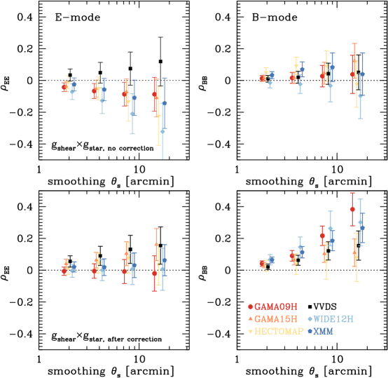
6 Simulations

In this section, we summarize the results of characterizing the shear catalog using simulated images. Two image simulation pipelines were used to address different problems, as described in the subsections below. These are completely distinct from the catalog-level simulations used to produce covariances in Section 3. While the results described below primarily serve as short summaries of the conclusions of separate papers, they are important to mention in this paper because the image simulations are our primary means to answer several critical questions about the shape catalog that cannot be directly or cleanly answered through other means: What is the rate of unrecognized blends? Do the measured shapes exhibit coherent alignments with bright objects due to image processing errors such as sky subtraction errors? What are the primary sources of shear calibration biases, and how can we quantify and correct for them? These are such critical elements of weak lensing science that we summarize the results of the simulation work and their main conclusions here.

6.1 Synthetic Object Pipeline

The HSC Synthetic Object Pipeline (hereafter SynPipe; Huang et al. 2017; Murata et al. in prep.) is a module that interfaces with hscPipe and which can be used to insert synthetic objects into real HSC images. This is a versatile simulation module that can be used for a variety of purposes such as evaluating the completeness of a survey and testing the robustness of photometry measurements. Of relevance to this paper, we use SynPipe to evaluate the overall performance of hscPipe, to estimate the level of galaxy blending within the HSC Wide survey, to perform independent cross-checks on the results from our GREAT3-like simulations (Section 6.2), and finally to evaluate the number of background galaxies lost to blending and masking effects around bright foreground galaxies (Medezinski et al., 2017).

The details of SynPipe are provided in Huang et al. (2017), and are briefly summarized here. SynPipe uses GalSim (Rowe et al., 2015) v1.4 as a backend to reliably create realizations of synthetic objects. These can be stars, galaxies described by single- or double-Sérsic models, or galaxies described by the sum of a de Vaucouleurs and an exponential profile. SynPipe is similar in spirit to the BALROG simulation package used for the DES survey as described by Suchyta et al. (2016), with two main differences. The first is that SynPipe interfaces with hscPipe and can therefore be used to create synthetic objects with properties measured in the same way as HSC data. Second, unlike BALROG, which inserts synthetic galaxies into co-added images, SynPipe operates by injecting synthetic objects directly into images at the single exposure level. Synthetic objects processed though SynPipe therefore go through the same detection, stacking, and measurement process as real stars and galaxies observed by HSC.

HSC is the deepest of the existing wide field lensing surveys. This means that HSC source galaxies will be subject to blending effects that may impact photo-$z$ and shear estimates and are hence a source of systematic error. In Murata et al. (in prep.), we use SynPipe to attempt to quantify the effects of galaxy blends for the HSC wide survey. We refer the reader to Murata et al. (in prep.) for the full details of our study, and briefly summarize our main findings here. Synthetic galaxies are classified into systems that are “cleanly” recovered versus those which are subject to unrecognized blending (this occurs when hscPipe was unable to deblend a synthetic galaxy from a neighbouring real galaxy due to the failure to recognize multiple peaks in the object). After imposing weak lensing cuts, we find that the unrecognized blend rate increases because unrecognized blends have increased flux and apparent size, leading them to scatter into our sample across the $i=24.5$ and $R_{2}=0.3$ cuts, which are the most relevant cuts for defining our sample (see figure 12).

It is important to note that the simulations from Section 6.2 that are used to quantify shear systematics (additive and multiplicative biases) include a realistic rate of unrecognized blends. This realistic unrecognized blend rate is achieved by including galaxies from space-based imaging with all surrounding structures, whether galaxies or stars, and relying on the HSC pipeline to detect, deblend, and select galaxies for weak lensing analysis. The simulations were then used to derive our multiplicative and additive shear bias corrections. Hence the impact of unrecognized blends on shear are already corrected for, while the impact on photometric redshift estimates cannot be studied with either set of simulations described in this section (because they are single-band only). The impact of unrecognized blends on photometric redshift estimation for the weak lensing sample is deferred to future work.

In Murata et al. (in prep.) we also search for evidence of “orientation” bias. This is an effect in which our detection algorithm may preferentially select galaxies with certain orientations in the vicinity of neighbouring bright galaxies or in which neighbouring bright galaxies may create a bias in our shape measurements. We find evidence for a strong orientation bias effect around bright galaxies with $i<21$. The shapes of synthetic galaxies preferentially point towards the locations of $i<21$ galaxies on scales below about 6 arcseconds (30 kpc at $z=0.4$), however this orientation bias is not present on larger scales. Because galaxy clusters contain many bright galaxies, it is possible that this orientation bias may affect cluster lensing studies, especially for lower redshift galaxy clusters.

6.2 GREAT3-like simulations

To estimate the level of ensemble shear biases such as noise bias, model bias, and bias due to intrinsic limitations of the re-Gaussianization method, and to estimate selection biases, we use a set of simulations that are similar in spirit to those used for the GREAT3 challenge (Mandelbaum et al., 2014, 2015) and that do not involve injecting objects into real data, unlike the SynPipe simulations. In these simulations, galaxies are placed on a $100\times 100$ grid with the same lensing shear applied to each galaxy on that grid and analyzed using hscPipe. Galaxies are simulated in 90-degree rotated pairs to cancel out the shape noise to lowest order. With a set of many such grids, it is possible to test the recovery of shears, including both additive and multiplicative biases.

In order to include a realistic level of blending, parent galaxy samples were defined using HSC survey data (with different observations that have different observing conditions) in the COSMOS field. By matching the HSC detections in that region against the HST-COSMOS images, and including a large chunk of the actual space-based image without attempting to mask out nearby objects, realistic galaxy morphologies, unrecognized blending effects, and contamination of light profiles by neighboring objects are naturally included in this simulation despite its grid configuration. We found that the failure to include nearby galaxies in the simulations meant that (a) the simulated galaxy population looked very different from the real one (galaxies too small compared to those that are observed), and (b) the shear calibration was over-estimated by a very large amount, $\sim 9$% when averaged over the entire sample.

After defining this parent galaxy sample, the simulations were produced in a way that is meant to represent coadded images. Full coadd PSF images were drawn from random locations in the survey, along with the sky variance at the same random locations. Using that set of random locations, it was possible to create a set of simulations with a distribution of observing conditions matching those in the real HSC survey. The parent galaxy sample from the HST-COSMOS images had the HST-COSMOS PSF deconvolved, then were sheared, convolved with the randomly-selected HSC PSFs, and resampled to the HSC pixel scale. Because of the image resampling and combination process, the noise in the coadds exhibits pixel-to-pixel correlations, but these correlations can be manipulated by adding a small amount of additional noise. Instead of fully whitening the noise, the average noise correlation function in the HSC coadds was measured and used to produce the noise fields in the simulations.

For more details of how these simulations were created, see Mandelbaum et al. (2017). As demonstrated there, the observed distribution of galaxy properties after following this procedure for producing the simulations looks remarkably similar to the distribution of object properties in the real HSC data, with the means of the $|e|$, $R_{2}$, magnitude, and SNR distributions in the simulations and data agreeing at the 0.1, 1, 1, and 5% level.

These simulations were used for four main purposes, resulting in the development of fitting formulae that were used to populate fields in the catalog and database:

1. Shape measurement error (i.e., statistical uncertainty in per-object shapes due to pixel noise): as demonstrated in, e.g., Reyes et al. (2012), the naive shape measurement errors from re-Gaussianization underestimate the real statistical errors by typically 30%. Using the multiple noise realizations of the same galaxy, we determined a fitting formula for shape measurement errors and their dependence on galaxy properties.

2. Intrinsic shape noise: the response of the ensemble average ellipticities (distortions) to lensing shears depends on the intrinsic shape noise. We used the shape measurement errors described previously, together with the observed shape dispersion in the real data, to produce a fitting formula for the intrinsic shape noise as a function of galaxy properties with typical $\sigma_{e}\sim 0.4$ or $\sigma_{\gamma}\sim 0.24$. These numbers increase at large $R_{2}$ likely due to the presence of unrecognized blends, which increase the intrinsic shape dispersion (Dawson et al., 2016).

3. Shear calibration bias: we tested the ensemble shear recovery using these simulations, and produced a fitting formulae for the average calibration bias as a function of galaxy properties. This can be used to correct the ensemble average shear estimated using subpopulations of the catalog for the sources of calibration bias listed above.

4. Additive biases: we also produced a fitting formula for the additive bias due to residual PSF anisotropy, i.e., $\hat{g}=(1+m)g+ae_{\text{PSF}}$. Using the formula for $a$ as a function of galaxy properties, and the PSF shape as a function of position in the survey, we can generate estimates of the additive bias per shape component for each galaxy. These numbers can be used as inputs to ensemble shear estimators.

Selection biases due to the quantities used for selecting galaxies (Section 5.1) correlating with the shear and/or PSF anisotropy can be a highly significant source of selection bias in ensemble shear estimation (e.g., Hirata et al., 2004; Mandelbaum et al., 2005; Jarvis et al., 2016). Fortunately, these simulations make it possible to estimate which quantities used for selection can generate a selection bias, and the magnitude of selection biases for subsamples of the catalog. There we ascertained using the simulations that without any additional selection criteria, the multiplicative selection bias due to our lower limit on resolution factor is $1.0\%\pm 0.3\%$, and presented a method for how to extend this result to subsamples of the catalog. We also found that multiplicative selection biases due to other cuts such as our magnitude cut are statistically consistent with zero, as are additive biases due to any of our cuts. Note that unlike the previously-discussed estimates, there is no per-object estimate of selection bias; by definition, it is only defined for ensembles. None of the plots in this paper are corrected for selection bias; corrections will be applied for each science paper depending on the sample used.

The conclusions of that work are that when considering model bias due to realistic galaxy morphology, noise bias, the impact of light from nearby objects, unrecognized blends, and selection bias due to weights and selection criteria applied to the sample, additive biases are controlled at a level well below the requirements given in this paper. The multiplicative bias corrections defined in that work were found to have a modest dependence on how the galaxy sample was defined, such that when applying additional cuts on photometric redshifts, the uncertainty in shear calibration may be as large as $\sim 1/3$ the requirements given in this paper. Factoring in these effects plus those mentioned above (sensitivity of the results to the galaxy population in the simulations), that work estimates a systematic uncertainty in the multiplicative shear calibration of 0.01, which is within our requirement of 0.017. As a consequence, additive or multiplicative biases due to shear systematics originating from the effects listed in this paragraph may be considered as controlled at the level of the requirements given in this paper.

While performing cosmological analyses with the shear catalogs, we will adopt a catalog level blinding approach which relies on manipulating the fitting formulae used to correct for the various biases mentioned above. In order to maintain this blinding, we do not provide the exact fitting formulae here.

7 Other tests related to image processing

In this section we show some additional tests of early stages of the image processing that could have an effect on shear systematics.

7.1 Sky subtraction

As shown in the SDSS (e.g., Aihara et al., 2011), errors in sky subtraction around bright objects (stars and galaxies) can cause systematic errors in the properties of faint nearby galaxies such as those that dominate our source catalog. This can result in inconsistent galaxy selection criteria in dense regions vs. the rest of the survey, coherent tangential shear biases around bright lens objects, and other systematic errors. Indeed, the HSC DR1 paper describes sky over-subtraction near bright galaxies, but the question of how this may result in coherent shear measurement systematics was not determined there.

One test of sky subtraction errors comes from the already-computed tangential shear profile around stars (after imposition of the bright star mask to remove regions that are badly affected by the light from bright stars). This was shown in figure 14, and demonstrates that there is no coherent tangential or radial shear around bright stars detected down to scales of $0.2$ arcmin. As discussed in Section 6.1, there are signs of orientation bias (coherent radial shear induced with respect to bright galaxies) in the source sample at separations of $\leq 6$, which could be a sign of sky subtraction issues on even smaller scales.

7.2 Relative astrometry

One potential source of systematic errors in shear is the coaddition process. Relative astrometric errors should lead to an additional blurring kernel in the stars and galaxies on the coadd (effectively another Gaussian convolution in the PSF), but the coadd PSF does not include this term. As shown in Section 4.2.1 we see no sign that the star images on the coadd are larger than the coadd PSF model – indeed, there is a $10^{-3}$-level discrepancy of the opposite sign – but nonetheless we can use the relative astrometric errors characterized in the HSC DR1 paper to estimate how important this effect may be for shear estimation.

As mentioned there, the internal astrometric accuracy is $\sim 10$ mas. Given a typical seeing size of $0.6$, and treating both the PSF and the blurring due to astrometric errors as Gaussians that can be added in quadrature, the effective PSF would be larger than the coadded PSF by 1 part in $10^{-4}$ (in terms of the linear size). Given that the systematic bias in the shear due to this effective PSF model size error would be a similar order of magnitude, we argue that this systematic error is subdominant to those discussed previously in this paper. This also explains why no signature of PSF broadening was seen in the tests of the coadded PSFs.

7.3 Star/galaxy separation

Failures in star/galaxy separation can cause two different types of systematic errors in weak lensing. First, if the sample of objects used to determine the PSF includes some small galaxies (or binary stars) then the PSF model will be systematically biased to larger size (and/or gain some spurious shape). Figure 13 of the HSC DR1 paper illustrates that the purity level of the bright star sample is very high. Here we rely on our direct empirical tests of PSF models that indicate that their sizes are sufficiently accurate to meet our requirements.

Second, if the shear catalog includes some stars or binary stars misidentified as galaxies, they will dilute the shear signal, resulting in a negative calibration bias. We assess the level of stellar contamination in the shear catalog using the HSC-COSMOS field, taking advantage of the HST observations also available in that region. The HSC-COSMOS data used here correspond to the HSC Deep survey layer, and hence individual exposure times are longer than in the Wide survey. Exposures with different seeing values were used to create Wide-depth stacks with effective seeing better than, around the median of, and worse than the HSC Wide layer on average. These stacks have seeing values of 0.5, 0.7, and 1.0, as described in Section 3.8 of the HSC DR1 paper, and have fewer exposures than in a typical Wide layer coadd due to the differences in exposure times.

We take as a reference the star-galaxy classification performed on the HST-COSMOS data by Leauthaud et al. (2007). Because these data are higher resolution than the HSC data, we regard the HST star catalog as the true, complete star catalog for our purposes. As shown in Leauthaud et al. (2007), the star-galaxy separation in HST-COSMOS is reliable down to a depth of $i\sim 25$, which is fainter than our shape catalog. We cross-match the two datasets in the COSMOS region with a maximum matching radius of $0.4$, which is smaller than the HSC PSF and which can be clearly distinguished as the distance at which spurious matches start to dominate the cross-matched catalog.

Figure 21 shows the fraction of objects in the shear catalogs constructed for each of these stacks that were classified as stars by Leauthaud et al. (2007). For typical seeing conditions, the contamination is below 0.2% for $i$-band magnitudes $<$22, increasing to about 0.5% for the faintest sources included in the shape catalog. Even in the worst seeing conditions (1), which are highly non-representative of the shear catalog overall, there is only a 1% contamination at the faintest magnitudes. For all three seeing conditions, the average over the catalog is at most 0.5% (0.3% for median seeing). We note that this low level of stellar contamination is due to a combination of the pipeline star/galaxy classifier and other cuts, such as the resolution cut, that is designed to remove objects (even galaxies) that are too poorly resolved for accurate shear estimation. Such contamination is well within the levels required for current science analyses, with the relevant requirement from Section 3 being $|\delta m|<0.017$. Our most relevant estimate is somewhere between the best and median seeing, given the seeing distribution of this catalog, and hence is about 15% of that requirement. For the current dataset we do not explore the stellar contamination or its impact on scientific results any further. We also note that the results are nearly indistinguishable with and without lensing weights.

Figure 21: Top: contamination of the shape catalog by stars incorrectly classified as galaxies by the HSC pipeline, calculated in the COSMOS field by comparing to a classification performed using HST data. We show the contamination as a function of $i$-band magnitude for three different values of seeing which are representative of good, typical and bad conditions across the HSC survey. Errorbars show Poisson uncertainties. Dotted lines show overall averages. Bottom: number of objects in each magnitude bin, for each dataset split by seeing. Both panels show unweighted results, however the results are nearly indistinguishable when incorporating the lensing weights.

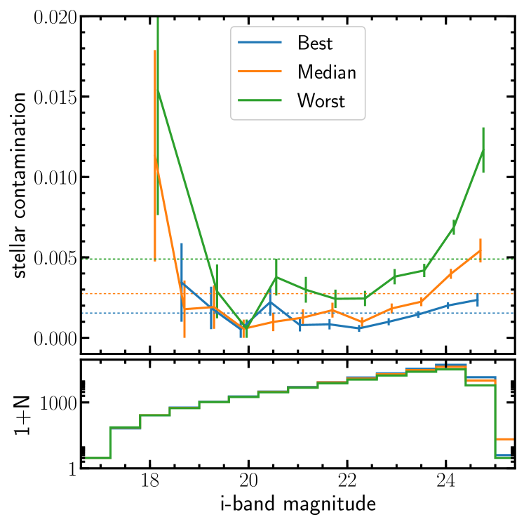
8 Photometric redshifts

Until now, we have focused exclusively on systematics related to shear estimation using the entire sample of galaxies for which shapes could be measured. In this section, we briefly comment on photometric redshifts, which are discussed in much more detail in Tanaka et al. (2017); Medezinski et al. (2017); Speagle et al. (in prep.); More et al. (in prep.). Our simulations analysis (Mandelbaum et al., 2017) will address the question of whether applying calibrations as a function of $S/N$ and resolution is sufficient to correct for redshift trends. In this paper, we focus on only the most basic aspects of photometric redshifts in the source catalog.

The first question is how the requirement that there be a photometric redshift available reduce the source number density. For one typical photometric redshift catalog out of the several available options, mlz (machine learning and photo-$z$), the requirement that there be a value of photometric redshift results in a 12% reduction in the source number density. However, this statement is method-dependent as will be explored by Speagle et al. (in prep.); More et al. (in prep.).

Next, we consider how photometric redshift cuts modify the observed distributions of galaxies properties, such as those shown in figure 12. For this purpose, we divide the source sample into three roughly equal subsamples by cutting at $z=0.6$ and $z=1$. Then we plot the lensing-weighted distributions of galaxy properties for the entire sample of galaxies with photo-$z$, and for those with photo-$z$ above $0.6$ and above $1.0$ (again using mlz). The resulting distributions are shown in figure 22. As shown, the distributions of resolution factor and distortion magnitude are not strongly modified when placing photometric redshift cuts, while requiring a higher photometric redshift skews the sample towards fainter magnitudes and lower signal-to-noise ratio. This suggests that shear biases such as noise bias will be the primary difference between source samples cut based on redshift, while effects that depend on the resolution factor distribution (e.g., the impact of PSF model size errors) will affect the samples similarly.

Figure 22: We show how the lensing-weighted distribution of galaxy properties across all survey fields combined changes when imposing lower limits on the photometric redshift from mlz. The resulting samples with these cuts are similar to those that might be used for tomographic analysis, or for galaxy-galaxy lensing source samples. Each panel shows a different galaxy property as labeled on the panel itself, and all distributions are renormalized to integrate to the same total.

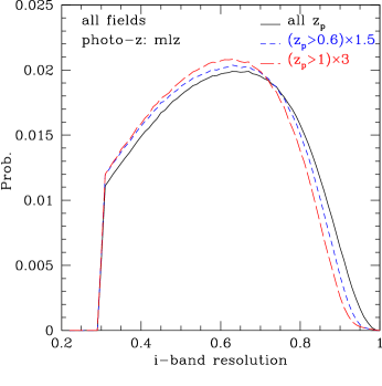
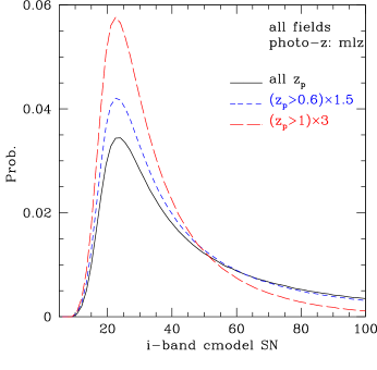
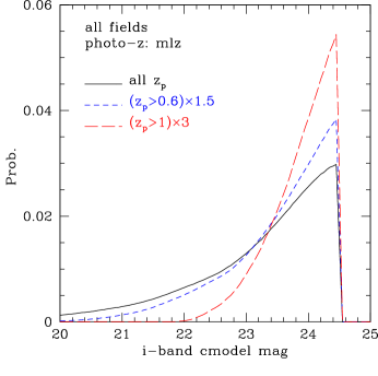
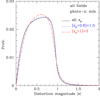
Finally, we note that we see evidence that the results of some null tests depend on the applied photo-$z$ cuts. Since this depends on the choice of photo-$z$ method and the cut itself, we defer tests of this effect to science papers, which will be motivated by more specific photo-$z$ cuts and will have null tests that depend on the science case.

While the impact of photometric redshift bias and scatter on the HSC weak lensing analysis is thoroughly quantified elsewhere (Medezinski et al., 2017; Speagle et al., in prep.; More et al., in prep.), and the biases in the signals depend on the adopted photometric redshift code, here we comment briefly on the current understanding of the residual systematic uncertainties (after correcting for known biases). As shown in Medezinski et al. (2017), when using a spectroscopic sample that has been reweighted to match the color and magnitude distribution of the weak lensing source sample, the calibration of lensing signals for samples with lenses at $z>0.4$ has an uncertainty of $\pm 2$%. This uncertainty is primarily statistical, and is driven by the limited size of spectroscopic samples covering the faint end of our source sample. This slightly exceeds the requirements given in Section 3 for constraints on the calibration of the lensing signals. There, the number given was that shear calibration must be known to better than 0.017 for it to avoid contributing significantly to the overall error budget. As this is a requirement on calibration, a similar requirement applies to uncertainty in lensing signal calibration due to photometric redshifts. Hence the results from Medezinski et al. (2017) suggest that our uncertainty in the calibration of the lensing signals due to photometric redshift uncertainties is a systematic that must be explicitly added to the error budget for cosmological weak lensing analysis with first-year data, due to it no longer being completely negligible compared to our statistical uncertainties. We caution that the specific values of this systematic uncertainty in Medezinski et al. (2017) are specific to the adopted $p(z)$ method and cuts in that work; for cosmological galaxy-galaxy lensing analyses, the same methodology will be applied to derive numbers that apply to that analysis (More et al., in prep.).

Ongoing spectroscopic campaigns such as the one described in Masters et al. (2017) will improve spectroscopic redshift coverage in areas of color and magnitude space where existing samples are relatively sparse, and thereby reduce this systematic uncertainty for future analyses. In addition, once a larger HSC survey area is available it will be possible to use clustering cross-correlations to reconstruct ensemble redshift distributions for photo-$z$-selected samples, as is used by the Dark Energy Survey as a cross-check to the spectroscopic sample reweighting presented in Hoyle et al. (2017).

9 Summary

In this paper, we have characterized the catalogs to be used for weak lensing science with the first data release of the HSC survey. These catalogs were produced using the moments-based re-Gaussianization method of PSF correction as applied to a linear coadd, for which the PSF model was constructed as a linear combination of the single-epoch PSF models. The tests of the quality of these catalogs presented in this paper are predominantly internal tests such as the calculation of standard weak lensing null tests. Some systematics cannot be assessed using null tests; these were only briefly summarized here, and are evaluated in detail in other work:

• Unrecognized blend rate as a function of galaxy properties, and spurious shear due to bright objects, are quantified using SynPipe in Murata et al. (in prep.).

• Multiplicative and additive biases due to the PSF correction algorithm used here, including model bias, noise bias, the impact of unrecognized blends, and selection biases, are quantified using simulations in Mandelbaum et al. (2017).

• The impact of photometric redshift errors (Tanaka et al., 2017) on weak lensing cosmology analyses are quantified in Medezinski et al. (2017); Speagle et al. (in prep.); More et al. (in prep.); Hikage et al. (in prep.).

Finally, null tests carried out at the map level in Oguri et al. (2017) by correlating the lensing mass maps against maps of quantities that can induce systematic error (e.g., PSF shape and size) produced null detections. These are nicely complementary to the null tests carried out in this paper at the level of 1- and 2-point correlation functions.

We emphasize that this work represents the technical underpinnings of HSC weak lensing science papers using this catalog only. Future data releases will cover more area and will be processed by a different software pipeline. As a result, the performance requirements become more stringent, but the results of the null tests and other tests to characterize performance of the catalog will also change. We particularly highlight the fact that several of our PSF model-related null tests (specifically the PSF model size residuals and $\rho_{1}$) meet our requirements with the current catalog, but would not meet the requirements for the full HSC survey area, which are a factor of $\sim 2.7$ more stringent. Of the improvements mentioned below in Section 9.2, the PSF model improvements are most clearly motivated by our current failure to meet the full-survey requirements on PSF model fidelity.

However, while our shear estimation method is not demonstrably producing multiplicative shear systematics that would exceed the full-survey requirement of $6\times 10^{-3}$, it seems unlikely that our simulation-based calibration method alone can reduce the shear calibration uncertainty much below our current uncertainty of $10^{-2}$. Hence, the difficulties in precise estimation of the shear calibration using simulations (rather than clearly evident systematics exceeding the full survey requirements) have motivated several of the shear methodology updates listed in Section 9.2 for future data releases. These methodology updates will result in us having two or three independent means of validating our shear calibration, providing the multiple cross-checks that will be needed to reduce that part of the systematic error budget.

9.1 Systematic error budget

In this section we present a brief quantitative summary of the elements of the systematic error budget, for which the key components are listed in Table 1 and the requirements themselves were derived in Section 3. For each row in the table, we discuss what systematic effects contribute and at what level.

The first row in the table is the uncertainty in the overall multiplicative bias in the galaxy-galaxy lensing signal. While the discussion in Section 3 focused primarily on multiplicative biases in shear, in principle any effect that causes a multiplicative bias would contribute to this row. The relevant effects discussed in this paper are (i) stellar contamination (Section 7.3), (ii) astrometric errors (Section 7.2), (iii) photometric redshift errors (Section 8 summarizing results from other work), and (iv) a range of shear-related multiplicative biases (Section 6.2 summarizing results from other work). Of these, (i), (ii), and (iv) were found to be below our requirements, but (iii) exceeds our nominal requirements and hence must be tracked as a separate, significant component of the systematic error budget.

The second row in the table is the uncertainty in the shear calibration due to uncertainty in PSF model size errors. As shown in Section 4.2, the mean of the PSF fractional size error (evaluated with the non-PSF star sample) is just barely within our requirement of $4\times 10^{-3}$. Hence this systematic error component should in principle be tracked as a component of the systematic error budget. However, as mentioned above, we already need to track the photometric redshift error contribution to the systematic error budget, and that contribution is several times the size of the PSF model size error, so when added in quadrature, the PSF model size error is relatively unimportant.

The remainder of Table 1 relates to additive biases. As discussed in Section 6.2, simulations have shown that additive bias due to insufficient correction for PSF anisotropy can be removed effectively to well within the requirements. The other major component of the additive biases can come from PSF model shape errors, for which we placed requirements on the five $\rho$ statistics. As shown in Section 4.2.2, the $\rho$ statistics in this catalog do satisfy our (conservative) requirements, though $\rho_{1}$ is quite close to the requirements. This is likely the source of the spurious star-galaxy shape correlation function presented in Section 5.3, which on most scales was subdominant to the expected cosmic shear signal, but may need to be modeled out on scales exceeding $1^{\circ}$ (which fortunately do not dominate our cosmological constraining power, due to the cosmic variance errorbars).

9.2 Areas for future improvement

In the near future, we anticipate that another shear catalog using a very different method of shear inference (an implementation of the Bayesian Fourier Domain or BFD algorithm from Bernstein et al. 2016) will be produced and cross-comparisons will be made with the catalog described in this paper, providing a complementary cross-check on the first year HSC shear estimation process with the older re-Gaussianization method. This will be valuable given the very different assumptions behind the two methods.

The results of the tests in this paper and in Bosch et al. (2017) suggest several avenues for improvement in future data releases, where contiguous regions of at least twice the size of the regions in DR1 will necessitate a better handling of systematics. We enumerate the highest priority plans here:

1. We would like to have at least two shear estimation algorithms available concurrently rather than in succession; work in other surveys (e.g., Jarvis et al., 2016) has demonstrated the power of ensemble shear cross-comparisons between two methods applied to the same dataset.

2. At least one method should operate at the level of individual exposures rather than coadds.

3. Rather than assessing shear calibration only via simulations, which are limited due to imperfect knowledge of the galaxy population, future data releases should use some implementation of the metacalibration method (Huff & Mandelbaum, 2017; Sheldon & Huff, 2017), which assesses the response of the shear estimation method to a shear via resimulation of the data itself.

4. We need improved methods of understanding the impact of unrecognized blends on photometric redshifts, given the high unrecognized blend rate in this dataset.

5. Given the dominant role of photometric redshift uncertainty in our systematic error budget, it will be important to have spectroscopic training samples with better coverage of the faint end of our galaxy sample, and use complementary methods such as clustering redshifts (Newman, 2008; Rahman et al., 2015) that benefit from having wider survey areas, as discussed in section 8.

6. The PSF models will need to be improved if we are to meet our requirements in future years, and to recover the best-seeing areas that were removed for this analysis. We anticipate that this will involve replacement of the algorithm rather than improvement of the existing algorithm; this is actively being worked on now.

9.3 Outlook for first-year HSC weak lensing science

For weak lensing analyses that will result directly in cosmological parameter constraints, we note that blinding has been recognized in recent years as a valuable method for reducing confirmation bias. For these analyses, the HSC weak lensing group is adopting a combination of catalog-level and analysis-level blinding schemes. However, the unblinded catalogs are being used directly for non-cosmological analyses. A more detailed discussion of the blinding method is deferred to cosmological analysis papers.

To summarize, for the systematics that can be characterized with null tests, the catalogs presented in this work meet the requirements for first-year weak lensing science with HSC. This paper has presented requirements on a broader set of weak lensing systematics than can be characterized with null tests; additional papers will detail the methods used to assess the systematics that were not fully addressed here, referring in all cases to the requirements defined in this paper. Other work has identified the weak lensing signal calibration uncertainty due to photometric redshift errors as a systematic that exceeds our nominal (conservative) requirements, and thus must be added as a separate term in the systematic error budget for cosmological weak lensing analyses. The tests in this work have helped us identify the dominant sources of systematic error that will have to be tracked in cosmological weak lensing analyses (as summarized in Section 9.1), and also were useful for identifying future avenues for improvement in subsequent shear catalogs.

In this special issue of PASJ, some initial weak lensing science papers will be presented covering topics such as cluster-galaxy lensing and mass mapping, with more to come (including cosmological analyses) in the following months. This begins an exciting new era of cosmological weak lensing analysis with the HSC survey. Also, this catalog will be released publicly when cosmological results are published. Details of data access will be made public at that time.

The Hyper Suprime-Cam (HSC) collaboration includes the astronomical communities of Japan and Taiwan, and Princeton University. The HSC instrumentation and software were developed by the National Astronomical Observatory of Japan (NAOJ), the Kavli Institute for the Physics and Mathematics of the Universe (Kavli IPMU), the University of Tokyo, the High Energy Accelerator Research Organization (KEK), the Academia Sinica Institute for Astronomy and Astrophysics in Taiwan (ASIAA), and Princeton University. Funding was contributed by the FIRST program from Japanese Cabinet Office, the Ministry of Education, Culture, Sports, Science and Technology (MEXT), the Japan Society for the Promotion of Science (JSPS), Japan Science and Technology Agency (JST), the Toray Science Foundation, NAOJ, Kavli IPMU, KEK, ASIAA, and Princeton University.

This paper makes use of software developed for the Large Synoptic Survey Telescope. We thank the LSST Project for making their code available as free software at http://dm.lsst.org.

The Pan-STARRS1 Surveys (PS1) have been made possible through contributions of the Institute for Astronomy, the University of Hawaii, the Pan-STARRS Project Office, the Max-Planck Society and its participating institutes, the Max Planck Institute for Astronomy, Heidelberg and the Max Planck Institute for Extraterrestrial Physics, Garching, The Johns Hopkins University, Durham University, the University of Edinburgh, Queen’s University Belfast, the Harvard-Smithsonian Center for Astrophysics, the Las Cumbres Observatory Global Telescope Network Incorporated, the National Central University of Taiwan, the Space Telescope Science Institute, the National Aeronautics and Space Administration under Grant No. NNX08AR22G issued through the Planetary Science Division of the NASA Science Mission Directorate, the National Science Foundation under Grant No. AST-1238877, the University of Maryland, and Eotvos Lorand University (ELTE) and the Los Alamos National Laboratory.

Based on data collected at the Subaru Telescope and retrieved from the HSC data archive system, which is operated by Subaru Telescope and Astronomy Data Center, National Astronomical Observatory of Japan.

We thank Josh Meyers, Paul Price, and the anonymous referee for helpful comments that improved the quality of this work. This work is in part supported by JSPS KAKENHI (Grant Number 26800093, 15H03654, and JP17H01131) as well as MEXT Grant-in-Aid for Scientific Research on Innovative Areas (No. 15H05887, 15H05892, 15H05893, 15K21733). RM is supported by the US Department of Energy Early Career Award Program. HM is supported by the Jet Propulsion Laboratory, California Institute of Technology, under a contract with the National Aeronautics and Space Administration. MS is supported by the University of California Riverside Office of Research and Economic Development through the FIELDS NASA-MIRO program. SM is supported by the Japan Society for Promotion of Science grants JP15K17600 and JP16H01089. RyM is financially supported by the University of Tokyo-Princeton strategic partnership grant and Advanced Leading Graduate Course for Photon Science (ALPS). WC is supported by the WFIRST program.

Appendix A Catalog quantities

The HSC first-year shape catalog is a set of three catalogs which share the same objects in the same order. The main catalog includes the object positions, photometry and shapes, as listed in Table LABEL:tab:shape_catalog. The photo-z information is stored in two different catalogs. The first includes the point estimates listed in Table 2 in Tanaka et al. (2017), and the other is the photo-$z$ PDF.

Table 3: Quantities in shape catalog.

Column	Meaning
Basic quantities and flags
object_id	object ID
ira	right ascension (J2000.0) measured in $i-$band
idec	declination (J2000.0) measured in $i-$band
tract	tract ID
patch	patch ID
weak_lensing_flag	weak lensing flag
merge_peak_[grizy]	peak detected in $grizy-$band
[grizy]countinputs	number of $grizy-$band visits contributing at center
iflags_pixel_bright_object_center/any	source center is close to/source footprint includes BRIGHT_OBJECT pixels
iblendedness_flags	flag set if iblendedness_abs_flux could not be measured because a required input was missing
iblendedness_abs_flux	measure of how flux is affected by neighbors
Photometry
a_[grizy]	Galactic extinction in $grizy-$band
iflux_kron, iflux_kron_err	kron flux in $i-$band, and its error
iflux_kron_flags	kron flux flag in $i-$band
imag_kron, imag_kron_err	kron magnitude in $i-$band, and its error
imag_kron_flags	kron magnitude flag in $i-$band
iflux_cmodel, iflux_cmodel_err	cmodel flux in $i-$band, and its error
iflux_cmodel_flags	cmodel flux flag in $i-$band
imag_cmodel, imag_cmodel_err	cmodel magnitude in $i-$band, and its error
imag_cmodel_flags	cmodel magnitude flag in $i-$band
[grizy]flux_forced_cmodel	forced cmodel flux in $grizy-$band
[grizy]flux_forced_cmodel_err	forced cmodel flux error in $grizy-$band
[grizy]flux_forced_cmodel_flags	forced cmodel flag in $grizy-$band (True indicates failure)
[grizy]mag_forced_cmodel	forced cmodel magnitude in $grizy-$band
[grizy]mag_forced_cmodel_err	forced cmodel magnitude error in $grizy-$band
[grizy]flux_forced_kron	forced kron flux in $grizy-$band
[grizy]flux_forced_kron_err	forced kron flux error in $grizy-$band
[grizy]flux_forced_kron_flags	forced kron flag in $grizy-$band (True indicates failure)
[grizy]mag_forced_kron	forced kron magnitude in $grizy-$band
[grizy]mag_forced_kron_err	forced kron magnitude error in $grizy-$band
Regaussianization shapes based on data alone
ishape_hsm_regauss_e1/e2	Distortion in sky coordinates estimated by regaussianization method defined
	in distortion, i.e., $|e|=(a^{2}-b^{2})/(a^{2}+b^{2})$.
ishape_hsm_regauss_sigma	non-calibrated shape measurement noise
ishape_hsm_regauss_resolution	resolution of galaxy image defined in equation (4)
Quantities related to regaussianization shapes calibrated based on image simulations
ishape_hsm_regauss_derived_weight	weight for galaxy shapes
ishape_hsm_regauss_derived_sigma_e	shape measurement noise
ishape_hsm_regauss_derived_rms_e	rms galaxy shape of a population of galaxies
ishape_hsm_regauss_derived_bias_m	multiplicative bias
ishape_hsm_regauss_derived_bias_c1	additive bias for $e_{1}$
ishape_hsm_regauss_derived_bias_c2	additive bias for $e_{2}$
Non PSF-corrected shapes
ishape_sdss_ixx/ixy/iyy	Adaptive moments in arcsec2
ishape_sdss_psf_ixx/ixy/iyy	Adaptive moments of PSF evaluated at object position in arcsec2

Appendix B Galaxy cuts

Table 4 lists the exact column names used to impose the galaxy selection criteria discussed in Section 5.1. All cuts are imposed in the $i$-band, as indicated by the ‘i’ in front of the flag names.

Cut	Meaning
Basic flag cuts
idetect$\_$is$\_$primary $==$ True	Identify unique detections only
ideblend$\_$skipped $==$ False	Deblender skipped this group of objects
iflags$\_$badcentroid $==$ False	Centroid measurement failed
icentroid$\_$sdss$\_$flags $==$ False	centroid.sdss measurement failed
iflags$\_$pixel$\_$edge $==$ False	Object too close to image boundary for reliable measurements
iflags$\_$pixel$\_$interpolated$\_$center $==$ False	A pixel flagged as interpolated is close to object center
iflags$\_$pixel$\_$saturated$\_$center $==$ False	A pixel flagged as saturated is close to object center
iflags$\_$pixel$\_$cr$\_$center $==$ False	A pixel flagged as a cosmic ray hit is close to object center
iflags$\_$pixel$\_$bad $==$ False	A pixel flagged as otherwise bad is close to object center
iflags$\_$pixel$\_$suspect$\_$center $==$ False	A pixel flagged as near saturation is close to object center
iflags$\_$pixel$\_$clipped$\_$any $==$ False	Flagged as source footprint includes clipped pixels
ishape$\_$hsm$\_$regauss$\_$flags $==$ False	Error code returned by shape measurement code
ishape$\_$hsm$\_$regauss$\_$sigma $!=$ NaN	Shape measurement uncertainty should not be NaN
iclassification$\_$extendedness $!=0$	Extended object
Cuts on object properties
iflux$\_$cmodel/iflux$\_$cmodel$\_$err $\geq 10$	Galaxy has high enough $S/N$ in $i$ band
ishape$\_$hsm$\_$regauss$\_$resolution $\geq 0.3$	Galaxy is sufficiently resolved
(ishape$\_$hsm$\_$regauss$\_$e1${}^{2}+$ishape$\_$hsm$\_$regauss$\_$e2${}^{2})^{1/2}<2$	Total distortion cut
$0\leq$ishape$\_$hsm$\_$regauss$\_$sigma $\leq 0.4$	Estimated shape measurement error is reasonable
imag$\_$cmodel $-$ a$\_$i $\leq 24.5$	Magnitude cut
iblendedness$\_$abs$\_$flux $<10^{-0.375}$	Avoid spurious detections and those contaminated by blends
Require that at least two of the following four cuts be passed (not all)
gflux$\_$cmodel/gflux$\_$cmodel$\_$err $\geq 5$	Galaxy has high enough $S/N$ in $g$ band
rflux$\_$cmodel/rflux$\_$cmodel$\_$err $\geq 5$	Galaxy has high enough $S/N$ in $r$ band
zflux$\_$cmodel/zflux$\_$cmodel$\_$err $\geq 5$	Galaxy has high enough $S/N$ in $z$ band
yflux$\_$cmodel/yflux$\_$cmodel$\_$err $\geq 5$	Galaxy has high enough $S/N$ in $y$ band

Table 4: Selection criteria imposed on the shape catalog, as described in Section 5.1. The flags marked ^* come with the following caveat: hscPipe does not propagate pixels affected by cosmic rays and sensor defects to the coadd, so the actual effect of these for our purposes is that the coadded PSF model (which never accounts for masked pixels) is subtly incorrect. Due to a bug hscPipe does not set these flags on coadd measurements at all, however, so at present including them here is a no-op; in later versions of hscPipe in which the bug is fixed, filtering on these flags will reject objects with incorrect PSF models.

Appendix C Shear estimation

Here we describe the procedure for using the entries in the shear catalog to calculate average shear signals. This calculation will use the following shorthand for these catalog entries from Table LABEL:tab:shape_catalog:

• Distortions $e_{1}$, $e_{2}$ in sky coordinates: ishape_hsm_regauss_e1/e2

• Shape weights $w$: ishape_hsm_regauss_derived_weight

• Intrinsic shape dispersion per component $e_{\text{rms}}$: ishape_hsm_regauss_derived_rms_e (these are defined for the population as a function of galaxy properties like SNR and resolution, and hence are not the same for each galaxy)

• Multiplicative bias $m$: ishape_hsm_regauss_derived_bias_m

• Additive biases $c_{1}$, $c_{2}$: ishape_hsm_regauss_derived_bias_c1/c2

C.1 Galaxy-galaxy lensing

C.1.1 Basic calculation

After using the $e_{1}$ and $e_{2}$ values to calculate tangential shear values $e_{t}$ over which one wishes to average to get galaxy-galaxy or cluster-galaxy lensing profiles, the average tangential shear profile can be calculated using the following formulae, where $i$ is used to indicate lens-source pairs and the calculation is typically done in bins of angle $\theta$ or physical separation $r_{p}$. For simplicity our notation does not explicitly indicate this binning, so the formulae presented should be read as being used for each bin with lens-source pairs already identified.

As described in Section 2.4, our distortion estimates do not provide an unbiased estimator for the shear; we need to calculate a responsivity factor ${\cal R}$. This can be calculated based on the inverse variance weights $w_{i}$ and the per-object estimates of RMS distortion $e_{\text{RMS},i}$ as

$${\cal R}=1-\frac{\sum_{i}w_{i}e_{\text{rms},i}^{2}}{\sum_{i}w_{i}}.$$ (39)

While this simplified formula can in principle induce some systematic error, the systematic error will automatically be corrected when we test shear estimation on the simulations.

We can use the catalog estimates of calibration bias $m_{i}$ to derive an ensemble estimate for the calibration bias for our sample:

$$\hat{m}=\frac{\sum_{i}w_{i}m_{i}}{\sum_{i}w_{i}}$$ (40)

Finally, these can be combined with the standard average over tangential shear estimates to get the stacked shear estimator

$$\hat{g}=\frac{\sum_{i}w_{i}e_{t,i}}{2{\cal R}(1+\hat{m})\sum_{i}w_{i}}.$$ (41)

C.1.2 Additive bias terms

In principle, additive systematic errors can induce scale-dependent additive biases in the stacked shear profiles, particularly if these vary across the sky and/or the signal is calculated on large scales, where many of the annuli around lenses will be incomplete due to survey boundaries. While this systematic can be removed by subtracting the signal around random lenses that are distributed with the same area coverage as the real lenses (e.g., Mandelbaum et al., 2013), such a correction depends on a clear understanding of the factors that determine the lens sample angular selection function (e.g., if the lens selection depends on observing conditions, this must be modeled). Use of the additive biases $c_{1,2}$ values in the catalog can be used to more directly remove the additive systematic due to incomplete correction for the PSF anisotropy, though some additive systematics due to PSF modeling errors and selection biases may remain. To construct the additive term that must be subtracted from $\hat{g}$, the following calculation must be done. First, the $c_{1,2}$ values must be rotated into the tangential frame in the lens-source pair system, just like the $e_{1,2}$ values, to get $c_{t}$. Then define the weighted sum

$$\hat{c}=\frac{\sum_{i}w_{i}c_{t,i}}{\sum_{i}w_{i}}.$$ (42)

Finally, $\hat{c}/(1+\hat{m})$ should be subtracted from the $\hat{g}$ from equation (41).

The order of operations defining how $\hat{m}$ and $\hat{c}$ should be used comes from defining shear calibration biases as

$$\frac{\sum_{i}w_{i}e_{t,i}}{2{\cal R}\sum_{i}w_{i}}=(1+\hat{m})g_{\text{true}}+\hat{c}.$$ (43)

The first step, dividing by $1+\hat{m}$, is used to define the shear estimator in equation (41). This definition explains why the additive term to be removed is $\hat{c}/(1+\hat{m})$ rather than $\hat{c}$.

C.2 Pair-weighted statistics

Some plots in this paper show pair-weighted statistics, such as the star-galaxy shape correlation function in figure 17. Here we describe how to adapt the above calculations to such pair-weighted statistics. The star-galaxy correlation involves pairs consisting of one star and one galaxy. Using the galaxy sample, we can use equations (39) and (40) to calculate the responsivity ${\cal R}$ and overall calibration bias $\hat{m}$, respectively. However, the additive bias requires a per-object correction. Hence for this case, we define a per-object galaxy shear estimate as

$$\hat{g}_{i}=\frac{1}{1+\hat{m}}\left[\frac{e_{i}}{2{\cal R}}-c_{i}\right]$$ (44)

and then the $\hat{g}_{i}$ values are correlated with the star shapes. For the star shapes, we index the stars with a subscript $j$, and define $\hat{g}_{j}^{*}=e_{j}/2$ (using the relation between distortion and shear for intrinsically round objects). We equally weight the stars, i.e., $w_{j}=1$, and hence our estimator for the star-galaxy shape correlation function is

$$\xi_{\text{sg}}=\frac{\sum_{i}\sum_{j}w_{i}w_{j}\hat{g}_{i}\hat{g}_{j}^{*}}{\sum_{i}\sum_{j}w_{i}w_{j}}=\frac{\sum_{i}\sum_{j}w_{i}\hat{g}_{i}\hat{g}_{j}^{*}}{\sum_{i}\sum_{j}w_{i}}$$ (45)

defined within bins of separation $\theta$.

C.3 Additional complications

Finally, we note that if additional weight factors are desired, for example, to weight by lens properties, or to get inverse variance-weighted $\Delta\Sigma$ profiles (which require weighting by $1/\Sigma_{\text{crit}}^{2}$), the weights must be self-consistently updated in all of equations throughout appendix C.

References

- Abazajian & Dodelson (2003) Abazajian, K., & Dodelson, S. 2003, Physical Review Letters, 91, 041301
- Abbott et al. (2016) Abbott, T., Abdalla, F. B., Allam, S., et al. 2016, Phys. Rev. D, 94, 022001
- Aihara et al. (2011) Aihara, H., Allende Prieto, C., An, D., et al. 2011, ApJS, 193, 29
- Aihara et al. (2017a) Aihara, H., Armstrong, R., Bickerton, S., et al. 2017a, ArXiv e-prints, arXiv:1702.08449 (HSC DR1 paper)
- Aihara et al. (2017b) Aihara, H., Arimoto, N., Armstrong, R., et al. 2017b, arXiv:1704.05858
- Alam et al. (2017) Alam, S., Miyatake, H., More, S., Ho, S., & Mandelbaum, R. 2017, MNRAS, 465, 4853
- Amara & Réfrégier (2008) Amara, A., & Réfrégier, A. 2008, MNRAS, 391, 228
- Annis et al. (2014) Annis, J., Soares-Santos, M., Strauss, M. A., et al. 2014, ApJ, 794, 120
- Antilogus et al. (2014) Antilogus, P., Astier, P., Doherty, P., Guyonnet, A., & Regnault, N. 2014, Journal of Instrumentation, 9, C03048
- Armstrong et al. (in prep.) Armstrong, R., et al. in prep.
- Axelrod et al. (2010) Axelrod, T., Kantor, J., Lupton, R. H., & Pierfederici, F. 2010, in Proc. SPIE, Vol. 7740, Software and Cyberinfrastructure for Astronomy, 774015
- Bacon et al. (2000) Bacon, D. J., Refregier, A. R., & Ellis, R. S. 2000, MNRAS, 318, 625
- Battaglia et al. (2016) Battaglia, N., Leauthaud, A., Miyatake, H., et al. 2016, J. Cosmology Astropart. Phys, 8, 013
- Becker et al. (2016) Becker, M. R., Troxel, M. A., MacCrann, N., et al. 2016, Phys. Rev. D, 94, 022002
- Behroozi et al. (2013) Behroozi, P. S., Wechsler, R. H., & Wu, H.-Y. 2013, ApJ, 762, 109
- Benabed & van Waerbeke (2004) Benabed, K., & van Waerbeke, L. 2004, Phys. Rev. D, 70, 123515
- Bernstein & Jain (2004) Bernstein, G., & Jain, B. 2004, ApJ, 600, 17
- Bernstein (2010) Bernstein, G. M. 2010, MNRAS, 406, 2793
- Bernstein & Armstrong (2014) Bernstein, G. M., & Armstrong, R. 2014, MNRAS, 438, 1880
- Bernstein et al. (2016) Bernstein, G. M., Armstrong, R., Krawiec, C., & March, M. C. 2016, MNRAS, 459, 4467
- Bernstein & Jarvis (2002) Bernstein, G. M., & Jarvis, M. 2002, AJ, 123, 583
- Bertin (2011) Bertin, E. 2011, in Astronomical Society of the Pacific Conference Series, Vol. 442, Astronomical Data Analysis Software and Systems XX, ed. I. N. Evans, A. Accomazzi, D. J. Mink, & A. H. Rots, 435
- Blake et al. (2016) Blake, C., Joudaki, S., Heymans, C., et al. 2016, MNRAS, 456, 2806
- Bonnett et al. (2016) Bonnett, C., Troxel, M. A., Hartley, W., et al. 2016, Phys. Rev. D, 94, 042005
- Bosch et al. (2017) Bosch, J., Armstrong, R., Bickerton, S., et al. 2017, ArXiv e-prints, arXiv:1705.06766
- Bridle et al. (2009) Bridle, S., Shawe-Taylor, J., Amara, A., et al. 2009, Annals of Applied Statistics, 3, 6
- Bridle et al. (2010) Bridle, S., Balan, S. T., Bethge, M., et al. 2010, MNRAS, 405, 2044
- Coulton et al. (in prep.) Coulton, W., et al. in prep.
- Coupon et al. (2017) Coupon, J., Czakon, N., Bosch, J., et al. 2017, ArXiv e-prints, arXiv:1705.00622
- Davis et al. (2007) Davis, M., Guhathakurta, P., Konidaris, N. P., et al. 2007, ApJ, 660, L1
- Dawson et al. (2013) Dawson, K. S., Schlegel, D. J., Ahn, C. P., et al. 2013, AJ, 145, 10
- Dawson et al. (2016) Dawson, W. A., Schneider, M. D., Tyson, J. A., & Jee, M. J. 2016, ApJ, 816, 11
- de Jong et al. (2013) de Jong, J. T. A., Verdoes Kleijn, G. A., Kuijken, K. H., & Valentijn, E. A. 2013, Experimental Astronomy, 35, 25
- Donahue et al. (2014) Donahue, M., Voit, G. M., Mahdavi, A., et al. 2014, ApJ, 794, 136
- Fenech Conti et al. (2017) Fenech Conti, I., Herbonnet, R., Hoekstra, H., et al. 2017, MNRAS, 467, 1627
- Furusawa et al. (in prep.) Furusawa, H., et al. in prep.
- Gruen et al. (2015) Gruen, D., Bernstein, G. M., Jarvis, M., et al. 2015, Journal of Instrumentation, 10, C05032
- Hamana et al. (2013) Hamana, T., Miyazaki, S., Okura, Y., Okamura, T., & Futamase, T. 2013, PASJ, 65, 104
- Heymans et al. (2006) Heymans, C., Van Waerbeke, L., Bacon, D., et al. 2006, MNRAS, 368, 1323
- Heymans et al. (2013) Heymans, C., Grocutt, E., Heavens, A., et al. 2013, MNRAS, 432, 2433
- Hikage et al. (in prep.) Hikage, C., et al. in prep.
- Hildebrandt et al. (2017) Hildebrandt, H., Viola, M., Heymans, C., et al. 2017, MNRAS, 465, 1454
- Hinshaw et al. (2013) Hinshaw, G., Larson, D., Komatsu, E., et al. 2013, ApJS, 208, 19
- Hirata & Seljak (2003) Hirata, C., & Seljak, U. 2003, MNRAS, 343, 459
- Hirata et al. (2004) Hirata, C. M., Mandelbaum, R., Seljak, U., et al. 2004, MNRAS, 353, 529
- Hoekstra et al. (2015) Hoekstra, H., Herbonnet, R., Muzzin, A., et al. 2015, MNRAS, 449, 685
- Hoekstra et al. (2002) Hoekstra, H., Yee, H. K. C., Gladders, M. D., et al. 2002, ApJ, 572, 55
- Høg et al. (2000) Høg, E., Fabricius, C., Makarov, V. V., et al. 2000, A&A, 355, L27
- Hoyle et al. (2017) Hoyle, B., Gruen, D., Bernstein, G. M., et al. 2017, ArXiv e-prints, arXiv:1708.01532
- Hu (2002) Hu, W. 2002, Phys. Rev. D, 65, 023003
- Huang et al. (2017) Huang, S., Leauthaud, A., Murata, R., et al. 2017, ArXiv e-prints, arXiv:1705.01599
- Huff & Mandelbaum (2017) Huff, E., & Mandelbaum, R. 2017, ArXiv e-prints, arXiv:1702.02600
- Huterer (2002) Huterer, D. 2002, Phys. Rev. D, 65, 63001
- Hwang et al. (2016) Hwang, H. S., Geller, M. J., Park, C., et al. 2016, ApJ, 818, 173
- Ishak et al. (2004) Ishak, M., Hirata, C. M., McDonald, P., & Seljak, U. 2004, Phys. Rev. D, 69, 083514
- Jarvis (2015) Jarvis, M. 2015, TreeCorr: Two-point correlation functions, Astrophysics Source Code Library, ascl:1508.007
- Jarvis et al. (2004) Jarvis, M., Bernstein, G., & Jain, B. 2004, MNRAS, 352, 338
- Jarvis et al. (2016) Jarvis, M., Sheldon, E., Zuntz, J., et al. 2016, MNRAS, 460, 2245
- Jee & Tyson (2011) Jee, M. J., & Tyson, J. A. 2011, PASP, 123, 596
- Jee et al. (2016) Jee, M. J., Tyson, J. A., Hilbert, S., et al. 2016, ApJ, 824, 77
- Joachimi et al. (2015) Joachimi, B., Cacciato, M., Kitching, T. D., et al. 2015, Space Sci. Rev., 193, 1
- Jurić et al. (2015) Jurić, M., Kantor, J., Lim, K., et al. 2015, ArXiv e-prints, arXiv:1512.07914
- Kacprzak et al. (2012) Kacprzak, T., Zuntz, J., Rowe, B., et al. 2012, MNRAS, 427, 2711
- Kaiser & Squires (1993) Kaiser, N., & Squires, G. 1993, ApJ, 404, 441
- Kaiser et al. (1995) Kaiser, N., Squires, G., & Broadhurst, T. 1995, ApJ, 449, 460
- Kiessling et al. (2015) Kiessling, A., Cacciato, M., Joachimi, B., et al. 2015, Space Sci. Rev., 193, 67
- Kilbinger (2015) Kilbinger, M. 2015, Reports on Progress in Physics, 78, 086901
- Kirk et al. (2015) Kirk, D., Brown, M. L., Hoekstra, H., et al. 2015, Space Sci. Rev., 193, 139
- Kitching et al. (2010) Kitching, T., Balan, S., Bernstein, G., et al. 2010, AOAS, 5, 2231
- Kitching et al. (2012) Kitching, T. D., Balan, S. T., Bridle, S., et al. 2012, MNRAS, 423, 3163
- Kwan et al. (2017) Kwan, J., Sánchez, C., Clampitt, J., et al. 2017, MNRAS, 464, 4045
- Laureijs et al. (2011) Laureijs, R., Amiaux, J., Arduini, S., et al. 2011, ArXiv e-prints, arXiv:1110.3193
- Le Fèvre et al. (2013) Le Fèvre, O., Cassata, P., Cucciati, O., et al. 2013, A&A, 559, A14
- Leauthaud et al. (2007) Leauthaud, A., Massey, R., Kneib, J.-P., et al. 2007, ApJS, 172, 219
- Leauthaud et al. (2010) Leauthaud, A., Finoguenov, A., Kneib, J.-P., et al. 2010, ApJ, 709, 97
- Leauthaud et al. (2017) Leauthaud, A., Saito, S., Hilbert, S., et al. 2017, MNRAS, 467, 3024
- LSST Science Collaboration et al. (2009) LSST Science Collaboration, Abell, P. A., Allison, J., et al. 2009, ArXiv e-prints, arXiv:0912.0201
- Lupton et al. (2001) Lupton, R., Gunn, J. E., Ivezić, Z., Knapp, G. R., & Kent, S. 2001, in Astronomical Society of the Pacific Conference Series, Vol. 238, Astronomical Data Analysis Software and Systems X, ed. F. R. Harnden, Jr., F. A. Primini, & H. E. Payne, 269
- Mandelbaum et al. (2013) Mandelbaum, R., Slosar, A., Baldauf, T., et al. 2013, MNRAS, 432, 1544
- Mandelbaum et al. (2005) Mandelbaum, R., Hirata, C. M., Seljak, U., et al. 2005, MNRAS, 361, 1287
- Mandelbaum et al. (2014) Mandelbaum, R., Rowe, B., Bosch, J., et al. 2014, ApJS, 212, 5
- Mandelbaum et al. (2015) Mandelbaum, R., Rowe, B., Armstrong, R., et al. 2015, MNRAS, 450, 2963
- Mandelbaum et al. (2017) Mandelbaum, R., Lanusse, F., Leauthaud, A., et al. 2017, preprint (arXiv:1710.00885), arXiv:1710.00885
- Massey et al. (2010) Massey, R., Kitching, T., & Richard, J. 2010, Reports on Progress in Physics, 73, 086901
- Massey et al. (2007a) Massey, R., Rowe, B., Refregier, A., Bacon, D. J., & Bergé, J. 2007a, MNRAS, 380, 229
- Massey et al. (2007b) Massey, R., Heymans, C., Bergé, J., et al. 2007b, MNRAS, 376, 13
- Massey et al. (2013) Massey, R., Hoekstra, H., Kitching, T., et al. 2013, MNRAS, 429, 661
- Masters et al. (2017) Masters, D. C., Stern, D. K., Cohen, J. G., et al. 2017, ApJ, 841, 111
- Mead et al. (2015) Mead, A. J., Peacock, J. A., Heymans, C., Joudaki, S., & Heavens, A. F. 2015, MNRAS, 454, 1958
- Medezinski et al. (2017) Medezinski, E., Oguri, M., Nishizawa, A. J., et al. 2017, arXiv:1706.00427
- Melchior et al. (2010) Melchior, P., Böhnert, A., Lombardi, M., & Bartelmann, M. 2010, A&A, 510, A75
- Melchior & Viola (2012) Melchior, P., & Viola, M. 2012, MNRAS, 424, 2757
- Miyazaki et al. (in prep.) Miyazaki, S., et al. in prep.
- More et al. (2015) More, S., Miyatake, H., Mandelbaum, R., et al. 2015, ApJ, 806, 2
- More et al. (2013) More, S., van den Bosch, F. C., Cacciato, M., et al. 2013, MNRAS, 430, 747
- More et al. (in prep.) More, S., et al. in prep.
- Murata et al. (in prep.) Murata, R., et al. in prep.
- Newman (2008) Newman, J. A. 2008, ApJ, 684, 88
- Oguri & Takada (2011) Oguri, M., & Takada, M. 2011, Phys. Rev. D, 83, 023008
- Oguri et al. (2017) Oguri, M., Miyazaki, S., Hikage, C., et al. 2017, ArXiv e-prints, arXiv:1705.06792
- Okabe & Smith (2016) Okabe, N., & Smith, G. P. 2016, MNRAS, 461, 3794
- Okabe et al. (2010) Okabe, N., Takada, M., Umetsu, K., Futamase, T., & Smith, G. P. 2010, PASJ, 62, 811
- Perlmutter et al. (1999) Perlmutter, S., Aldering, G., Goldhaber, G., et al. 1999, ApJ, 517, 565
- Pickles & Depagne (2010) Pickles, A., & Depagne, É. 2010, PASP, 122, 1437
- Pierre et al. (2016) Pierre, M., Pacaud, F., Adami, C., et al. 2016, A&A, 592, A1
- Rahman et al. (2015) Rahman, M., Ménard, B., Scranton, R., Schmidt, S. J., & Morrison, C. B. 2015, MNRAS, 447, 3500
- Refregier et al. (2012) Refregier, A., Kacprzak, T., Amara, A., Bridle, S., & Rowe, B. 2012, MNRAS, 425, 1951
- Reid et al. (2016) Reid, B., Ho, S., Padmanabhan, N., et al. 2016, MNRAS, 455, 1553
- Reyes et al. (2012) Reyes, R., Mandelbaum, R., Gunn, J. E., et al. 2012, MNRAS, 425, 2610
- Rhodes et al. (2001) Rhodes, J., Refregier, A., & Groth, E. J. 2001, ApJ, 552, L85
- Riess et al. (1998) Riess, A. G., Filippenko, A. V., Challis, P., et al. 1998, AJ, 116, 1009
- Rowe (2010) Rowe, B. 2010, MNRAS, 404, 350
- Rowe et al. (2015) Rowe, B. T. P., Jarvis, M., Mandelbaum, R., et al. 2015, Astronomy and Computing, 10, 121
- Samuroff et al. (2017) Samuroff, S., Troxel, M. A., Bridle, S. L., et al. 2017, MNRAS, 465, L20
- Schneider et al. (2015) Schneider, M. D., Hogg, D. W., Marshall, P. J., et al. 2015, ApJ, 807, 87
- Sheldon & Huff (2017) Sheldon, E. S., & Huff, E. M. 2017, ApJ, 841, 24
- Shirasaki et al. (2017) Shirasaki, M., Takada, M., Miyatake, H., et al. 2017, MNRAS, 470, 3476
- Shirasaki & Yoshida (2014) Shirasaki, M., & Yoshida, N. 2014, ApJ, 786, 43
- Shirasaki et al. (in prep.) Shirasaki, M., et al. in prep.
- Speagle et al. (in prep.) Speagle, J., et al. in prep.
- Spergel et al. (2015) Spergel, D., Gehrels, N., Baltay, C., et al. 2015, ArXiv e-prints, arXiv:1503.03757
- Suchyta et al. (2016) Suchyta, E., Huff, E. M., Aleksić, J., et al. 2016, MNRAS, 457, 786
- Swetz et al. (2011) Swetz, D. S., Ade, P. A. R., Amiri, M., et al. 2011, ApJS, 194, 41
- Takada & Hu (2013) Takada, M., & Hu, W. 2013, Phys. Rev. D, 87, 123504
- Takada & Jain (2004) Takada, M., & Jain, B. 2004, MNRAS, 348, 897
- Takada & White (2004) Takada, M., & White, M. 2004, ApJ, 601, L1
- Takahashi et al. (2017) Takahashi, R., Hamana, T., Shirasaki, M., et al. 2017, ArXiv e-prints, arXiv:1706.01472
- Tanaka et al. (2017) Tanaka, M., Coupon, J., Hsieh, B.-C., et al. 2017, ArXiv e-prints, arXiv:1704.05988
- Thornton et al. (2016) Thornton, R. J., Ade, P. A. R., Aiola, S., et al. 2016, ApJS, 227, 21
- Troxel & Ishak (2015) Troxel, M. A., & Ishak, M. 2015, Phys. Rep., 558, 1
- van den Bosch et al. (2013) van den Bosch, F. C., More, S., Cacciato, M., Mo, H., & Yang, X. 2013, MNRAS, 430, 725
- Van Waerbeke et al. (2000) Van Waerbeke, L., Mellier, Y., Erben, T., et al. 2000, A&A, 358, 30
- Van Waerbeke et al. (2013) Van Waerbeke, L., Benjamin, J., Erben, T., et al. 2013, MNRAS, 433, 3373
- Voigt & Bridle (2010) Voigt, L. M., & Bridle, S. L. 2010, MNRAS, 404, 458
- von der Linden et al. (2014) von der Linden, A., Mantz, A., Allen, S. W., et al. 2014, MNRAS, 443, 1973
- Weinberg et al. (2013) Weinberg, D. H., Mortonson, M. J., Eisenstein, D. J., et al. 2013, Phys. Rep., 530, 87
- White et al. (2011) White, M., Blanton, M., Bolton, A., et al. 2011, ApJ, 728, 126
- Zacharias et al. (2004) Zacharias, N., Monet, D. G., Levine, S. E., et al. 2004, in Bulletin of the American Astronomical Society, Vol. 36, American Astronomical Society Meeting Abstracts, 1418
- Zentner et al. (2013) Zentner, A. R., Semboloni, E., Dodelson, S., et al. 2013, Phys. Rev. D, 87, 043509
- Zhang & Komatsu (2011) Zhang, J., & Komatsu, E. 2011, MNRAS, 414, 1047