Algorithms for $\ell_{p}$ Low-Rank Approximation

Abstract

We consider the problem of approximating a given matrix by a low-rank matrix so as to minimize the entrywise $\ell_{p}$-approximation error, for any $p\geq 1$; the case $p=2$ is the classical SVD problem. We obtain the first provably good approximation algorithms for this version of low-rank approximation that work for every value of $p\geq 1$, including $p=\infty$. Our algorithms are simple, easy to implement, work well in practice, and illustrate interesting tradeoffs between the approximation quality, the running time, and the rank of the approximating matrix.

1 Introduction

The problem of low-rank approximation of a matrix is usually studied as approximating a given matrix by a matrix of low rank so that the Frobenius norm of the error in the approximation is minimized. The Frobenius norm of a matrix is obtained by taking the sum of the squares of the entries in the matrix. Under this objective, the optimal solution is obtained using the singular value decomposition (SVD) of the given matrix. Low-rank approximation is useful in large data analysis, especially in predicting missing entries of a matrix by projecting the row and column entities (e.g., users and movies) into a low-dimensional space. In this work we consider the low-rank approximation problem, but under the general entrywise $\ell_{p}$ norm, for any $p\in[1,\infty]$.

There are several reasons for considering the $\ell_{p}$ version of low-rank approximation instead of the usually studied $\ell_{2}$ (i.e., Frobenius) version. For example, it is widely acknowledged that the $\ell_{1}$ version is more robust to noise and outliers than the $\ell_{2}$ version [2, 13, 24]. Several data mining and computer vision-related applications exploit this insight and resort to finding a low-rank approximation to minimize the $\ell_{1}$ error [15, 16, 20, 22]. Furthermore, the $\ell_{1}$ error is typically used as a proxy for capturing sparsity in many applications including robust versions of PCA, sparse recovery, and matrix completion; see, for example [2, 23]. For these reasons the problem has already received attention [10] and was suggested as an open problem by Woodruff in his survey on sketching techniques for linear algebra [21]. Likewise, the $\ell_{\infty}$ version (dubbed also as the Chebyshev norm) has been studied for the past many years [11, 12], though to the best of our knowledge, no result with theoretical guarantees was known for $\ell_{\infty}$ before our work. Our algorithm is also quite general, and works for every $p\geq 1$.

Working with $\ell_{p}$ error, however, poses many technical challenges. First of all, unlike $\ell_{2}$, the general $\ell_{p}$ space is not amenable to spectral techniques. Secondly, the $\ell_{p}$ space is not as nicely behaved as the $\ell_{2}$ space, for example, it lacks the notion of orthogonality. Thirdly, the $\ell_{p}$ version quickly runs into computational complexity barriers: for example, even the rank-$1$ approximation in $\ell_{1}$ has been shown to be NP-hard by Gillis and Vavasis [10]. However, there has been no dearth in terms of heuristics for the $\ell_{p}$ low-rank approximation problem, in particular for $p=1$ and $p=\infty$: this includes alternating convex (and, in fact, linear) minimization [14], methods based on expectation-maximization [19], minimization with augmented Lagrange multipliers [26], hyperplanes projections and linear programming [1], and generalizations of the Wiberg algorithm [6]. These heuristics, unfortunately, do not come with any performance guarantees. Polynomial-time algorithms for the general problem of rank-$k$ approximation has been stated as an open problem [21]. While theoretical approximation guarantees have been given for the rank-$1$ version for the $GF(2)$ and the Boolean cases [3], to the best of our knowledge there have been no provably good (approximation) algorithms for general matrices, or for rank more than one, or for general $\ell_{p}$.

1.1 Our Contributions

In this paper we obtain the first provably good algorithms for the $\ell_{p}$ rank-$k$ approximation problem for every $p\geq 1$. Let $n\times m$ be the dimensions of the input matrix. From an algorithmic viewpoint, there are three quantities of interest: the running time of the algorithm, the approximation factor guaranteed by the algorithm, and the actual number of vectors in the low-rank approximation that is output by the algorithm (even though we only desire $k$).

Given this setting, we show three main algorithmic results intended for the case when $k$ is not too large. First, we show that one can obtain a $(k+1)$-approximation to the rank-$k$ problem in time $m^{k}\operatorname{poly}(n,m)$; note that this running time is not polynomial once $k$ is larger than a constant. To address this, next we show that one can get an $O(k)$-approximation to the best $k$-factorization in time $O(\operatorname{poly}(nm))$; however, the algorithm returns $O(k\log m)$ columns, which is more than the desired $k$ (this is referred to as a bi-criteria approximation). Finally, we combine these two algorithms. We first show that the output of the second algorithm can further be refined to output exactly $k$ vectors, with an approximation factor of $\operatorname{poly}(k)$ and a running time of $O(\operatorname{poly}(n,m)(k\log n)^{k})$. The running time now is polynomial as long as $k=O(\log n/\log\log n)$. Next, we show that for any constant $p\geq 1$, we can obtain approximation factor $(k\log m)^{O(p)}$ and a running time of $\operatorname{poly}(n,m)$ for every value of $k$.

Our first algorithm is existential in nature: it shows that there are $k$ columns in the given matrix that can be used, along with an appropriate convex program, to obtain a $(k+1)$-approximation. Realizing this as an algorithm would therefore naïvely incur a factor $m^{k}$ in the running time. Our second algorithm works by sampling columns and iteratively “covering” the columns of the given matrix, for an appropriate notion of covering. In each round of sampling our algorithm uniformly samples from a remaining set of columns; we note here that it is critical that our algorithm is adaptive as otherwise uniform sampling would not work. While this is computationally efficient and maintains an $O(k)$-approximation to the best rank-$k$ approximation, it can end up with more than $k$ columns, in fact $O(k\log m)$. Our third algorithm fixes this issue by combining the first algorithm with the notion of a near-isoperimetric transformation for the $\ell_{p}$-space, which lets us transform a given matrix into another matrix spanning the same subspace but with small $\ell_{p}$ distortion.

A useful feature of our algorithms is that they are uniform with respect to all values of $p$. We test the performance of our algorithms, for $p=1$ and $p=\infty$, on real and synthetic data and show that they produce low-rank approximations that are substantially better than what the SVD (i.e., $p=2$) would obtain.

1.2 Related Work

In [18], a low-rank approximation was obtained which holds for every $p\in[1,2]$. Their main result is an $(O(\log m)\operatorname{poly}(k))$-approximation in $\operatorname{nnz}(A)+(n+m)\operatorname{poly}(k)$ time, for every $k$, where $\operatorname{nnz}(A)$ is the number of non-zero entries in $A$. In our work, we also obtain such a result for $p\in[1,2]$ via very different sampling-based methods, whereas the results in [18] are sketching-based. In addition to that, we obtain an algorithm with a $\operatorname{poly}(k)$ approximation factor which is independent of $m$ and $n$, though this latter algorithm requires $k=O(\log n/\log\log n)$ in order to be polynomial time.

Another result in  [18] shows how to achieve a $k\operatorname{poly}(\log k)$-approximation, in $n^{O(k)}$ time for $p\in[1,2]$. For $k$ larger than a constant, this is larger than polynomial time, whereas our algorithm with $\operatorname{poly}(k)$ approximation ratio is polynomial time for $k$ as large as $\Theta(\log n/\log\log n)$.

Importantly, our results hold for every $p\geq 1$, rather than only $p\in[1,2]$, so for example, include $p=\infty$.

In addition we note that there exist papers solving problems that, at first blush, might seem similar to ours. For instance, [5] study a convex relation, and a rounding algorithm to solve the subspace approximation problem (an $\ell_{p}$ generalization of the least squares fit), which is related to but different from our problem. Also, [7] offer a bi-criteria solution for another related problem of approximating a set of points by a collection of flats; they use convex relaxations to solve their problem and are limited to bi-criteria solutions, unlike ours. Finally, in some special settings robust PCA can be used to solve $\ell_{1}$ low-rank approximation [2]. However, robust PCA and $\ell_{1}$ low-rank approximation have some apparent similarities but they have key differences. Firstly, $\ell_{1}$ low-rank approximation allows to recover an approximating matrix of any chosen rank, whereas RPCA returns some matrix of some unknown (possibly full) rank. While variants of robust PCA have been proposed to force the output rank to be a given value [17, 25], these variants make additional noise model and incoherence assumptions on the input matrix, whereas our results hold for every input matrix. Secondly, in terms of approximation quality, it is unclear if near-optimal solutions of robust PCA provide near-optimal solutions for $\ell_{1}$ low-rank approximation.

Finally, we mention concrete example matrices $A$ for which the SVD gives a poor approximation factor for $\ell_{p}$-approximation error. First, suppose $p<2$ and $k=1$. Consider the following $n\times n$ block diagonal matrix composed of two blocks: a $1\times 1$ matrix with value $n$ and an $(n-1)\times(n-1)$ matrix with all $1$s. The SVD returns as a solution the first column, and therefore incurs polynomial in $n$ error for $p=2-\Omega(1)$. Now suppose $p>2$ and $k=1$. Consider the following $n\times n$ block diagonal matrix composed of two blocks: a $1\times 1$ matrix with value $n-2$ and an $(n-1)\times(n-1)$ matrix with all $1$s. The SVD returns as a solution the matrix spanned by the bottom block, and so also incurs an error polynomial in $n$ for $p=2+\Omega(1)$.

2 Background

For a matrix $M$, let $M_{i,j}$ denote the entry in its $i$th row and $j$th column and let $M_{i}$ denote its $i$th column. Let $M^{T}$ denote its transpose and let $|M|_{p}=\left(\sum_{i,j}|M_{i,j}|^{p}\right)^{1/p}$ denote its entry-wise $p$ norm. Given a set $S=\{i_{1},\ldots,i_{t}\}$ of column indices, let $M_{S}=M_{i_{1},\ldots,i_{t}}$ be the matrix composed of the columns of $M$ with the indices in $S$.

Given a matrix $M$ with $m$ columns, we will use $\operatorname{\mbox{\sl span}}M=\left\{\sum_{i=1}^{m}\alpha_{i}M_{i}\mid\alpha_{i}\in\mathbb{R}\right\}$ to denote the vectors spanned by its columns. If $M$ is a matrix and $v$ is a vector, we let $d_{p}(v,M)$ denote the minimum $\ell_{p}$ distance between $v$ and a vector in $\operatorname{\mbox{\sl span}}M$:

$$d_{p}(v,M)=\inf_{w\in\operatorname{\mbox{\sl span}}M}|v-w|_{p}.$$

Let $A\in\mathbb{R}^{n\times m}$ denote the input matrix and let $k>0$ denote the target rank. We assume, without loss of generality (w.l.o.g.), that $m\leq n$. Our first goal is, given $A$ and $k$, to find a subset $U\in\mathbb{R}^{n\times k}$ of $k$ columns of $A$ and $V\in\mathbb{R}^{k\times m}$ so as to minimize the $\ell_{p}$ error, $p\geq 1$, given by

$$|A-UV|_{p}.$$

Our second goal is, given $A$ and $k$, to find $U\in\mathbb{R}^{n\times k},V\in\mathbb{R}^{k\times m}$ to minimize the $\ell_{p}$ error, $p\geq 1$, given by

$$|A-UV|_{p}.$$

Note that in the second goal, we do not require $U$ be a subset of columns.

We refer to the first problem as the $k$-columns subset selection problem in the $\ell_{p}$ norm, denoted ${k}$-CSS_p, and to the second problem as the rank-$k$ approximation problem in the $\ell_{p}$ norm, denoted ${k}$-LRA_p. In the paper we often call $U,V$ the $k$-factorization of $A$. Note that a solution to ${k}$-CSS_p can be used as a solution to ${k}$-LRA_p, but not necessarily vice-versa.

In this paper we focus on solving the two problems for general $p$. Let $U^{\star}V^{\star}$ be a $k$-factorization of $A$ that is optimal in the $\ell_{p}$ norm, where $U^{\star}\in\mathbb{R}^{n\times k}$ and $V^{\star}\in\mathbb{R}^{k\times m}$, and let $\text{opt}_{k,p}(A)=|A-U^{\star}V^{\star}|_{p}$. An algorithm is said to be an $\alpha$-approximation, for an $\alpha\geq 1$, if it outputs $U\in\mathbb{R}^{n\times k},V\in\mathbb{R}^{k\times m}$ such that

$$|A-UV|_{p}\leq\alpha\cdot\mathrm{opt}_{k,p}(A).$$

It is often convenient to view the input matrix as $A=U^{\star}V^{\star}+\Delta=A^{\star}+\Delta$, where $\Delta$ is some error matrix of minimum $\ell_{p}$-norm. Let $\delta=|\Delta|_{p}=\mathrm{opt}_{k,p}(A)$.

We will use the following observation.

Lemma 1.

Let $U\in\mathbb{R}^{n\times k}$ and $v\in\mathbb{R}^{n\times 1}$. Suppose that there exists $x\in\mathbb{R}^{k\times 1}$ such that $\delta=\left|U\cdot x-v\right|_{p}$. Then, there exists a polynomial time algorithm that, given $U$ and $v$, finds $y\in\mathbb{R}^{k\times 1}$ such that $\left|U\cdot y-v\right|_{p}\leq\delta$.

Proof.

This $\ell_{p}$ regression problem is a convex program and well-known to be solvable in polynomial time. ∎

3 An $(m^{k}\operatorname{poly}(nm))$-time algorithm for ${k}$-LRA_p

In this section we will present an algorithm that runs in time $m^{k}\operatorname{poly}(nm)$ and produces a $(k+1)$-approximation to ${k}$-CSS_p (so also to ${k}$-LRA_p) of a matrix $A\in\mathbb{R}^{n\times m}$, $m\leq n$, for any $p\in[1,\infty]$. The algorithm simply tries all possible subsets of $k$ columns of $A$ for producing one of the factors, $U$, and then uses Lemma 1 to find the second factor $V$.

3.1 The existence of one factor in $A$

For simplicity, we assume that $|\Delta_{i}|_{p}>0$ for each column $i$. To satisfy this, we can add an arbitrary small random error to each entry of the matrix. For instance, for any $\gamma>0$, and to each entry of the matrix, we can add an independent uniform value in $[-\gamma,\gamma]$. This would guarantee that $|\Delta_{i}|_{p}>0$ for each $i\in[m]$.

Recall that $A=A^{\star}+\Delta$ is the perturbed matrix, and we only have access to $A$, not $A^{\star}$. Consider Algorithm 1 and its output $S$. Note that we cannot actually run this algorithm since we do not know $A^{\star}$. Thus, it is a hypothetical algorithm used for the purpose of our proof. That is, the algorithm serves as a proof that there exists a subset of $k$ columns of $A$ providing a good low rank approximation. In Theorem 3 we prove that the columns in $A$ indexed by the subset $S$ can be used as one factor of a $k$-factorization of $A$.

0:  A rank $k$ matrix $A^{\star}$ and perturbation matrix $\Delta$

0:  $k$ column indices of $A^{\star}$

1:  For each column index $i$, let $\tilde{A}^{\star}_{i}\leftarrow A^{\star}_{i}/|\Delta_{i}|_{p}$.

2:  Write $\tilde{A}^{\star}=\tilde{U}\cdot\tilde{V}$, s.t. $\tilde{U}\in\mathbb{R}^{n\times k},\tilde{V}\in\mathbb{R}^{k\times m}$.

3:  Let $S$ be the subset of $k$ columns of $\tilde{V}\in\mathbb{R}^{k\times m}$ that has maximum determinant in absolute value (note that the subset $S$ indexes a $k\times k$ submatrix).

4:  Output $S$.

Algorithm 1 Enumerating and selecting $k$ columns of $A$.

Before proving the main theorem of the subsection, we show a useful property of the matrix $\tilde{A}^{\star}$, that is, the matrix having the vector $A^{\star}_{i}/|\Delta_{i}|_{p}$ as the $i$th column. Then we will use this property to prove Theorem 3.

Lemma 2.

For each column $\tilde{A}^{\star}_{i}$ of $\tilde{A}^{\star}$, one can write $\tilde{A}^{\star}_{i}=\sum_{j\in S}M_{i}(j)\tilde{A}^{\star}_{j}$, where $|M_{i}(j)|\leq 1$ for all $i,j$.

Proof.

Fix an $i\in\{1,\ldots,m\}$. Consider the equation $\tilde{V}_{S}M_{i}=\tilde{V}_{i}$ for $M_{i}\in\mathbb{R}^{k}$. We can assume the columns in $\tilde{V}_{S}$ are linearly independent, since w.l.o.g., $\tilde{A}^{\star}$ has rank $k$. Hence, there is a unique solution $M_{i}=(\tilde{V}_{S})^{-1}\tilde{V}_{i}$. By Cramer’s rule, the $j$th coordinate $M_{i}(j)$ of $M_{i}$ satisfies $M_{i}(j)=\frac{\det(\tilde{V}^{j}_{S})}{\det(\tilde{V}_{S})}$, where $\tilde{V}^{j}_{S}$ is the matrix obtained by replacing the $j$th column of $\tilde{V}_{S}$ with $\tilde{V}_{i}$. By our choice of $S$, $|\det(\tilde{V}^{j}_{S})|\leq|\det(\tilde{V}_{S})|$, which implies $|M_{i}(j)|\leq 1$. Multiplying both sides of equation $\tilde{V}_{S}M_{i}=\tilde{V}_{i}$ by $\tilde{U}$, we have $\tilde{A}^{\star}_{S}M_{i}=\tilde{A}^{\star}_{i}$. ∎

Now we prove the main theorem of this subsection.

Theorem 3.

Let $U=A_{S}$. For $p\in[1,\infty]$, let $M_{1},\ldots,M_{m}$ be the vectors whose existence is guaranteed by Lemma 2 and let $V\in\mathbb{R}^{k\times n}$ be the matrix having the vector $|\Delta_{i}|_{p}\cdot\left(M_{i}(1)/|\Delta_{i_{1}}|_{p},\ldots,M_{i}(k)/|\Delta_{i_{k}}|_{p}\right)^{T}$ as its $i$th column. Then, $|A_{i}-(UV)_{i}|_{p}\leq(k+1)|\Delta_{i}|_{p}$ and hence $|A-UV|_{p}\leq(k+1)|\Delta|_{p}$.

Proof.

We consider the generic column $(UV)_{i}$.

$$(UV)_{i}\enspace=\enspace|\Delta_{i}|_{p}\sum_{j=1}^{k}\left(\frac{M_{i}(j)}{|\Delta_{i_{j}}|_{p}}A_{i_{j}}\right)$$

$$= |\Delta_{i}|_{p}\sum_{j=1}^{k}\left(\frac{M_{i}(j)}{|\Delta_{i_{j}}|_{p}}\left(A^{\star}_{i_{j}}+\Delta_{i_{j}}\right)\right)$$

$$= |\Delta_{i}|_{p}\sum_{j=1}^{k}\left(M_{i}(j)\tilde{A}^{\star}_{i_{j}}+M_{i}(j)\frac{\Delta_{i_{j}}}{|\Delta_{i_{j}}|_{p}}\right)$$

$$= |\Delta_{i}|_{p}\tilde{A}^{\star}_{i}+|\Delta_{i}|_{p}\sum_{j=1}^{k}\left(M_{i}(j)\frac{\Delta_{i_{j}}}{|\Delta_{i_{j}}|_{p}}\right)$$

$$= A^{\star}_{i}+\sum_{j=1}^{k}\left(|\Delta_{i}|_{p}\cdot M_{i}(j)\frac{\Delta_{i_{j}}}{|\Delta_{i_{j}}|_{p}}\right)\stackrel{{\scriptstyle\Delta}}{{=}}A^{\star}_{i}+E_{i}.$$

Observe that $E_{i}$ is the weighted sum of $k$ vectors, $\frac{\Delta_{i_{1}}}{|\Delta_{i_{1}}|_{p}},\ldots,\frac{\Delta_{i_{k}}}{|\Delta_{i_{k}}|_{p}}$, having unit $\ell_{p}$-norm. Observe further that, since the sum of their weights satisfies $|\Delta_{i}|_{p}\sum_{j=1}^{k}|M_{i}(j)|\leq k|\Delta_{i}|_{p}$, we have the $\ell_{p}$-norm of $E_{i}$ is not larger than $|E_{i}|_{p}\leq k|\Delta_{i}|_{p}$. The proof is complete using the triangle inequality:

$$|A_{i}-(UV)_{i}|_{p} \leq |A^{\star}_{i}-A_{i}|_{p}+|A^{\star}_{i}-(UV)_{i}|_{p}$$

$$= |\Delta_{i}|_{p}+|E_{i}|_{p}$$

$$\leq (k+1)|\Delta_{i}|_{p}.\quad\qed$$

3.2 An $m^{k}\operatorname{poly}(nm)$-time algorithm

In this section we give an algorithm that returns a $(k+1)$-approximation to the ${k}$-LRA_p problem in time $m^{k}\operatorname{poly}(nm)$.

0:  An integer $k$ and a matrix $A$

0:  $U\in\mathbb{R}^{n\times k},V\in\mathbb{R}^{k\times m}$ s.t. $|A-UV|_{p}\leq(k+1)\mathrm{opt}_{k,p}(A)$.

1:  for all $I\in\binom{[m]}{k}$ do

2:     Let $U=A_{I}$

3:     Use Lemma 1 to compute a matrix $V$ that minimizes the distance $d_{I}=|A-UV|_{p}$

4:  end for

5:  Return $U,V$ that minimizes $d_{I}$, for $I\in\binom{[m]}{k}$

Algorithm 2 A $(k+1)$-approximation to ${k}$-LRA_p.

The following statement follows directly from the existence of $k$ columns in $A$ that make up a factor $U$ having small $\ell_{p}$ error (Theorem 3).

Theorem 4.

Algorithm 2 obtains a $(k+1)$-approximation to ${k}$-LRA_p in time $m^{k}\operatorname{poly}(nm)$.

4 A $\operatorname{poly}(nm)$-time bi-criteria algorithm for ${k}$-CSS_p

We next show an algorithm that runs in time $\operatorname{poly}(nm)$ but returns $O(k\log m)$ columns of $A$ that can be used in place of $U$, with an error $O(k)$ times the error of the best $k$-factorization. In other words, it obtains more than $k$ columns but achieves a polynomial running time; we will later build upon this algorithm in Section 5 to obtain a faster algorithm for the ${k}$-LRA_p problem. We also show a lower bound: there exists a matrix $A$ for which the best possible approximation for the ${k}$-CSS_p, for $p\in(2,\infty)$, is $k^{\Omega(1)}$.

Definition 5 (Approximate coverage).

Let $S$ be a subset of $k$ column indices. We say that column $A_{i}$ is $c_{p}$-approximately covered by $S$ if for $p\in[1,\infty)$ we have $\min_{x\in\mathbb{R}^{k\times 1}}|A_{S}x-A_{i}|_{p}^{p}\leq c\frac{100(k+1)^{p}|\Delta|_{p}^{p}}{n}$, and for $p=\infty$, $\min_{x\in\mathbb{R}^{k\times 1}}|A_{S}x-A_{i}|_{\infty}\leq c(k+1)|\Delta|_{\infty}$. If $c=1$, we say $A_{i}$ is covered by $S$.

We first show that if we select a set $R$ columns of size $2k$ uniformly at random in $\binom{[m]}{2k}$, with constant probability we cover a constant fraction of columns of $A$.

Lemma 6.

Suppose $R$ is a set of $2k$ uniformly random chosen columns of $A$. With probability at least $2/9$, $R$ covers at least a $1/10$ fraction of columns of $A$.

Proof.

Let $i$ be a column index of $A$ selected uniformly at random and not in the set $R$. Let $T=R\cup\{i\}$ and let $\eta$ be the cost of the best $\ell_{p}$ rank-$k$ approximation to $A_{T}$. Note that $T$ is a uniformly random subset of $2k+1$ columns of $A$.

Case: $p<\infty$. Since $T$ is a uniformly random subset of $2k+1$ columns of $A$, ${\bf E}_{T}[\eta^{p}]=\frac{(2k+1)|\Delta|_{p}^{p}}{n}$. Let $\mathcal{E}_{1}$ denote the event “$\eta^{p}\leq\frac{10(2k+1)|\Delta|_{p}^{p}}{n}$”. By a Markov bound, $\Pr[\mathcal{E}_{1}]\geq 9/10$.

By Theorem 3, there exists a subset $L$ of $k$ columns of $A_{T}$ for which $\min_{X}|A_{L}X-A_{T}|_{p}^{p}\leq(k+1)^{p}\eta^{p}$. Since $i$ is itself uniformly random in the set $T$, it holds that ${\bf E}_{i}[\min_{x}|A_{L}x-A_{i}|_{p}^{p}\leq\frac{(k+1)^{p}\eta^{p}}{2k+1}$. Let $\mathcal{E}_{2}$ denote the event “$\min_{x}|A_{L}x-A_{i}|_{p}^{p}\leq\frac{10(k+1)^{p}\eta^{p}}{2k+1}$”. By a Markov bound, $\Pr[\mathcal{E}_{2}]\geq 9/10$.

Let $\mathcal{E}_{3}$ denote the event “$i\notin L$”. Since $i$ is uniformly random in the set $T$, $\Pr[\mathcal{E}_{3}]\geq\frac{k+1}{2k}>1/2$.

Clearly $\Pr[\mathcal{E}_{1}\wedge\mathcal{E}_{2}\wedge\mathcal{E}_{3}]\geq 3/10$. Conditioned on $\mathcal{E}_{1}\wedge\mathcal{E}_{2}\wedge\mathcal{E}_{3}$, we have

$$\min_{x}|A_{R}x-A_{i}|_{p}^{p} \stackrel{{\scriptstyle\mathcal{E}_{3}}}{{\leq}} \min_{x}|A_{L}x-A_{i}|_{p}^{p}$$

$$\stackrel{{\scriptstyle\mathcal{E}_{2}}}{{\leq}} \frac{10(k+1)^{p}\eta^{p}}{2k+1}$$

$$\stackrel{{\scriptstyle\mathcal{E}_{1}}}{{\leq}} \frac{100(k+1)^{p}|\Delta|_{p}^{p}}{n},$$

which implies that $i$ is covered by $R$. Note that the first inequality uses that $L$ is a subset of $R$ given $\mathcal{E}_{3}$, and so the regression cost using $A_{L}$ cannot be smaller than that of using $A_{R}$

Let $Z_{i}$ be an indicator variable if $i$ is covered by $R$ and let $Z=\sum_{i}Z_{i}$. We have ${\bf E}[Z]=\sum_{i}{\bf E}[Z_{i}]\geq\sum_{i}\frac{3}{10}=3m/10$; hence ${\bf E}[m-Z]\leq\frac{7m}{10}$. By a Markov bound, $\Pr[m-Z\geq\frac{9m}{10}]\leq\frac{7}{9}$.

Case $p=\infty$. Then $\eta\leq|\Delta|_{\infty}$ since $A_{T}$ is a submatrix of $A$. By Theorem 3, there exists a subset $L$ of $k$ columns of $A_{T}$ for which $\min_{X}|A_{L}X-A_{T}|_{\infty}\leq(k+1)\eta$. Defining $\mathcal{E}_{3}$ as before and conditioning on it, we have

$$\min_{x}|A_{R}x-A_{i}|_{\infty} \leq \min_{x}|A_{L}x-A_{i}|_{\infty}$$

$$\leq \min_{X}|A_{L}X-A_{T}|_{\infty}$$

$$\leq (k+1)|\Delta|_{\infty},$$

i.e., $i$ is covered by $R$. Again defining $Z_{i}$ to be the event that $i$ is covered by $R$, we have ${\bf E}[Z_{i}]\geq\frac{1}{2}$, and so ${\bf E}[m-Z]\leq\frac{m}{2}$, which implies $\Pr[m-Z\geq\frac{9m}{10}]\leq\frac{5}{9}<\frac{7}{9}$. ∎

We are now ready to introduce Algorithm 3. We can without loss of generality assume that the algorithm knows a number $N$ for which $|\Delta|_{p}\leq N\leq 2|\Delta|_{p}$. Indeed, such a value can be obtained by first computing $|\Delta|_{2}$ using the SVD. Note that although one does not know $\Delta$, one does know $|\Delta|_{2}$ since this is the Euclidean norm of all but the top $k$ singular values of $A$, which one can compute from the SVD of $A$. Then, note that for $p<2$, $|\Delta|_{2}\leq|\Delta|_{p}\leq n^{2-p}|\Delta|_{2}$, while for $p\geq 2$, $|\Delta|_{p}\leq|\Delta|_{2}\leq n^{1-2/p}|\Delta|_{p}$. Hence, there are only $O(\log n)$ values of $N$ to try, given $|\Delta|_{2}$, one of which will satisfy $|\Delta|_{p}\leq N\leq 2|\Delta|_{p}$. One can take the best solution found by Algorithm 3 for each of the $O(\log n)$ guesses to $N$.

0:  An integer $k$, and a matrix $A=A^{\star}+\Delta$.

0:  $O(k\log m)$ columns of $A$

   SelectColumns ($k,A$)

  if number of columns of $A\leq 2k$ then

     return all the columns of $A$

  else

     repeat

        Let $R$ be uniform at random $2k$ columns of $A$

     until at least $(1/10)$-fraction columns of $A$ are $c_{p}$-approximately covered

     Let $A_{\overline{R}}$ be the columns of $A$ not approximately covered by $R$

     return $A_{R}\cup$ SelectColumns ($k,A_{\overline{R}}$)

  end if

Algorithm 3 Selecting $O(k\log m)$ columns of $A$.

Theorem 7.

With probability at least $9/10$, Algorithm 3 runs in time $\operatorname{poly}(nm)$ and returns $O(k\log m)$ columns that can be used as a factor of the whole matrix inducing $\ell_{p}$ error $O(k|\Delta|_{p})$.

Proof.

First note, that if $|\Delta|_{p}\leq N\leq 2|\Delta|_{p}$ and if $i$ is covered by a set $R$ of columns, then $i$ is $c_{p}$-approximately covered by $R$ for a constant $c_{p}$; here $c_{p}=2^{p}$ for $p<\infty$ and $c_{\infty}=2$. By Lemma 6, the expected number of repetitions of selecting $2k$ columns until $(1/10)$-fraction of columns of $A$ are covered is $O(1)$. When we recurse on SelectColumns on the resulting matrix $A_{\overline{R}}$, each such matrix admits a rank-$k$ factorization of cost at most $|\Delta|_{p}$. Moreover, the number of recursive calls to SelectColumns can be upper bounded by $\log_{10}m$. In expectation there will be $O(\log m)$ total repetitions of selecting $2k$ columns, and so by a Markov bound, with probability $9/10$, the algorithm will choose $O(k\log m)$ columns in total and run in time $\operatorname{poly}(nm)$.

Let $S$ be the union of all columns of $A$ chosen by the algorithm. Then for each column $i$ of $A$, for $p\in[1,\infty)$, we have $\min_{x}|A_{S}x-A_{i}|_{p}^{p}\leq\frac{100(k+1)^{p}2^{p}|\Delta|_{p}^{p}}{n}$, and so $\min_{X}|A_{S}X-A|_{p}^{p}\leq 100(k+1)^{p}2^{p}|\Delta|_{p}^{p}$. For $p=\infty$ we instead have $\min_{x}|A_{S}x-A_{i}|_{\infty}\leq 2(k+1)|\Delta|_{\infty}$, and so $\min_{X}|A_{S}X-A|_{\infty}\leq 2(k+1)|\Delta|_{\infty}$. ∎

4.1 A lower bound for ${k}$-CSS_p

In this section we prove an existential result showing that there exists a matrix for which the best approximation to the ${k}$-CSS_p is $k^{\Omega(1)}$.

Lemma 8.

There exists a matrix $A$ such that the best approximation for the ${k}$-CSS_p problem, for $p\in(2,\infty)$, is $k^{\Omega(1)}$.

Proof.

Consider $A=(k+1)I_{k+1}$, where $I_{k+1}$ is the $(k+1)\times(k+1)$ identity matrix. And consider the matrix $B=(k+1)\cdot I_{k+1}-E$, where $E$ is the $(k+1)\times(k+1)$ all ones matrix. Note that $B$ has rank at most $k$, since the sum of its columns is $0$.

Case: $2<p<\infty$. If we choose any $k$ columns of $A$, then the $\ell_{p}$ cost of using them to approximate $A$ is $(k+1)$. On the other hand, $|A-B|_{\infty}=1$, which means that $\ell_{p}$ cost of $B$ is smaller or equal than $\left((k+1)^{2}\right)^{1/p}$.

Case: $p=\infty$. If we choose any $k$ columns of $A$, then the $\ell_{\infty}$ cost of using them to approximate $A$ is $k+1$. On the other hand, $|A-B|_{\infty}=1$, which means that $\ell_{\infty}$ cost of $B$ is smaller or equal than $1$. ∎

Note also that in [18] the authors show that for $p=1$ the best possible approximation is $\Omega(\sqrt{k})$ up to $\operatorname{poly}(\log k)$ factors.

5 A $((k\log n)^{k}\operatorname{poly}(mn))$-time algorithm for ${k}$-LRA_p

In the previous section we have shown how to get a rank-$O(k\log m)$, $O(k)$-approximation in time $\operatorname{poly}(nm)$ to the ${k}$-CSS_p and ${k}$-LRA_p problems. In this section we first show how to get a rank-$k$, $\operatorname{poly}(k)$-approximation efficiently starting from a rank-$O(k\log m)$ approximation. This algorithm runs in polynomial time as long as $k=O\left(\frac{\log n}{\log\log n}\right)$. We then show how to obtain a $(k\log m)^{O(p)}$-approximation ratio in polynomial time for every $k$.

Let $U$ be the columns of $A$ selected by Algorithm 3.

5.1 An isoperimetric transformation

The first step of our proof is to show that we can modify the selected columns of $A$ to span the same space but to have small distortion. For this, we need the following notion of isoperimetry.

Definition 9 (Almost isoperimetry).

A matrix $B\in\mathbb{R}^{n\times m}$ is almost-$\ell_{p}$-isoperimetric if for all $x$, we have

$$\frac{|x|_{p}}{2m}\leq|Bx|_{p}\leq|x|_{p}.$$

We now show that given a full rank $A\in\mathbb{R}^{n\times m}$, it is possible to construct in polynomial time a matrix $B\in\mathbb{R}^{n\times m}$ such that $A$ and $B$ span the same space and $B$ is almost-$\ell_{p}$-isoperimetric.

Lemma 10.

Given a full (column) rank $A\in\mathbb{R}^{n\times m}$, there is an algorithm that transforms $A$ into a matrix $B$ such that $\operatorname{\mbox{\sl span}}A=\operatorname{\mbox{\sl span}}B$ and $B$ is almost-$\ell_{p}$-isoperimetric. Furthermore the running time of the algorithm is $poly(nm)$.

Proof.

In [4], specifically, Equation (4) in the proof of Theorem 4, the authors show that in polynomial time it is possible to find a matrix $B$ such that $\operatorname{\mbox{\sl span}}B=\operatorname{\mbox{\sl span}}A$ and for all $x$,

$$|x|_{2}\leq|Bx|_{p}\leq\sqrt{m}|x|_{2},$$

for any $p\geq 1$.

If $p<2$, their result implies

$$\frac{|x|_{p}}{\sqrt{m}}\leq|x|_{2}\leq|Bx|_{p}\leq\sqrt{m}|x|_{2}\leq\sqrt{m}|x|_{p},$$

and so rescaling $B$ by $\sqrt{m}$ makes it almost-$\ell_{p}$-isoperimetric. On the other hand, if $p>2$, then

$$|x|_{p}\leq|x|_{2}\leq|Bx|_{p}\leq\sqrt{m}|x|_{2}\leq m|x|_{p},$$

and rescaling $B$ by $m$ makes it almost-$\ell_{p}$-isoperimetric. ∎

Note that the algorithm used in [4] relies on the construction of the Löwner–John ellipsoid for a specific set of points. Interestingly, we can also show that there is a more simple and direct algorithm to compute such a matrix $B$; this may be of independent interest. We provide the details of our algorithm in the supplementary material.

5.2 Reducing the rank to $k$

The main idea for reducing the rank is to first apply the almost-$\ell_{p}$-isoperimetric transformation to the factor $U$ to obtain a new factor $Z^{0}$. For such a $Z^{0}$, the $\ell_{p}$-norm of $Z^{0}V$ is at most the $\ell_{p}$-norm of $V$. Using this fact we show that $V$ has a low-rank approximation and a rank-$k$ approximation of $V$ translates into a good rank-$k$ approximation of $UV$. But a good rank-$k$ approximation of $V$ can be obtained by exploring all possible $k$-subsets of rows of $V$, as in Algorithm 2. More formally, in Algorithm 4 we give the pseudo-code to reduce the rank of our low-rank approximation from $O(k\log m)$ to $k$. Let $\delta=|\Delta|_{p}=\mathrm{opt}_{k,p}(A)$.

0:  $U\in\mathbb{R}^{n\times O(k\log m)}$, $V\in\mathbb{R}^{O(k\log m)\times m}$

0:  $W\in\mathbb{R}^{n\times k}$, $Z\in\mathbb{R}^{k\times m}$

1:  Apply Lemma 10 to $U$ to obtain matrix $W^{0}$

2:  Apply Lemma 1 to obtain matrix $Z^{0}$, s.t. $\forall i$, $|W^{0}Z^{0}_{i}-(UV)_{i}|_{p}$ is minimized

3:  Apply Algorithm 2 with input $(Z^{0})^{T}\in\mathbb{R}^{n\times O(k\log m)}$ and $k$ to obtain $X$ and $Y$

4:  Set $Z\leftarrow X^{T}$

5:  Set $W\leftarrow W^{0}Y^{T}$

6:  Output $W$ and $Z$

Algorithm 4 An algorithm that transforms an $O(k\log m)$-rank matrix decomposition into a $k$-rank matrix decomposition without inflating the error too much.

Theorem 11.

Let $A\in\mathbb{R}^{n\times m}$, $U\in\mathbb{R}^{n\times O(k\log m)}$, $V\in\mathbb{R}^{O(k\log m)\times m}$ be such that $|A-UV|_{p}=O(k\delta)$. Then, Algorithm 4 runs in time $O(k\log m)^{k}(mn)^{O(1)}$ and outputs $W\in\mathbb{R}^{n\times k},Z\in\mathbb{R}^{k\times m}$ such that $|A-WZ|_{p}=O((k^{4}\log k)\delta)$.

Proof.

We start by bounding the running time. Step $3$ is computationally the most expensive since it requires to execute a brute-force search on the $O(k\log m)$ columns of $(Z^{0})^{T}$. So the running time follows from Theorem 4.

Now we have to show that the algorithm returns a good approximation. The main idea behind the proof is that $UV$ is a low-rank approximable matrix. So after applying Lemma 10 to $U$ to obtain a low-rank approximation for $UV$ we can simply focus on $Z^{0}\in\mathbb{R}^{O(k\log m)\times n}$. Next, by applying Algorithm 2 to $Z^{0}$, we obtain a low-rank approximation in time $O(k\log m)^{k}(mn)^{O(1)}$. Finally we can use this solution to construct the solution to our initial problem.

We know by assumption that $|A-UV|_{p}=O(k\delta)$. Therefore, it suffices by the triangle inequality to show $|UV-WZ|_{p}=O((k^{4}\log k)\delta)$. First note that $UV=W^{0}Z^{0}$ since Lemma 10 guarantees that $\operatorname{\mbox{\sl span}}U=\operatorname{\mbox{\sl span}}W^{0}$. Hence we can focus on proving $|W^{0}Z^{0}-WZ|_{p}\leq O((k^{4}\log k)\delta)$.

We first prove two useful intermediate steps.

Lemma 12.

There exist matrices $U^{*}\in\mathbb{R}^{n\times k}$, $V^{*}\in\mathbb{R}^{k\times m}$ such that $|W^{0}Z^{0}-U^{*}V^{*}|_{p}=O(k\delta)$.

Proof.

There exist $U^{*}\in\mathbb{R}^{n\times k}$, $V^{*}\in\mathbb{R}^{k\times m}$ such that $|A-U^{*}V^{*}|_{p}\leq\delta$ and, furthermore, $|A-UV|_{p}=|A-W^{0}Z^{0}|_{p}=O(k\delta)$. The claim follows by the Minkowski inequality. ∎

Lemma 13.

There exist matrices $F\in\mathbb{R}^{O(k\log m)\times k}$, $D\in\mathbb{R}^{k\times n}$ such that $|W^{0}(Z^{0}-FD)|_{p}=O(k^{2}\delta)$.

Proof.

From Lemma 12, we know that $|W^{0}Z^{0}-U^{*}V^{*}|_{p}=O(k\delta)$. Hence, from Theorem 3, we know that there exists a matrix $C\in\mathbb{R}^{n\times k}$ composed of $k$ columns of $W^{0}Z^{0}$, and a matrix $D\in\mathbb{R}^{k\times m}$ such that $|W^{0}Z^{0}-CD|_{p}=O(k^{2}\delta)$. Furthermore, note that selecting $k$ columns of $W^{0}Z^{0}$ is equivalent to select the same columns in $Z^{0}$ and multiplying them by $W^{0}$. So we can express $C=W^{0}F$ for some matrix $F\in\mathbb{R}^{O(k\log m)\times k}$. Thus we can rewrite

$$|W^{0}Z^{0}-CD|_{p} = |W^{0}Z^{0}-W^{0}FD|_{p}$$

$$= |W^{0}(Z^{0}-FD)|_{p}$$

$$\leq O(k^{2}\delta).\quad\qed$$

Now from the guarantees of Lemma 10 we know that for any vector $y$, $|W^{0}y|_{p}\leq\frac{|y|_{p}}{k\log k}$. So we have $|Z^{0}-FD|_{p}\leq O((k^{3}\log k)\delta)$, Thus $|(Z^{0})^{T}-D^{T}F^{T}|_{p}\leq O((k^{3}\log k)\delta)$, so $(Z^{0})^{T}$ has a low-rank approximation with error at most $O((k^{3}\log k)\delta)$. So we can apply Theorem 3 again and we know that there are $k$ columns of $(Z^{0})^{T}$ such that the low-rank approximation obtained starting from those columns has error at most $O((k^{4}\log k)\delta)$. We obtain such a low-rank approximation from Algorithm 2 with input $(Z^{0})^{T}\in\mathbb{R}^{n\times O(k\log m)}$ and $k$. More precisely, we obtain an $X\in\mathbb{R}^{n\times k}$ and $Y\in\mathbb{R}^{k\times O(k\log m)}$ such that $|(Z^{0})^{T}-XY|_{p}\leq O((k^{4}\log k)\delta)$. Thus $|Z^{0}-Y^{T}X^{T}|_{p}\leq O((k^{4}\log k)\delta)$.

Now using again the guarantees of Lemma 10 for $W^{0}$, we get $|W^{0}(Z^{0}-Y^{T}X^{T})|_{p}\leq O((k^{4}\log k)\delta)$. So $|W^{0}(Z^{0}-Y^{T}X^{T})|_{p}=|W^{0}Z^{0}-WZ)|_{p}=|UV-WZ)|_{p}\leq O((k^{4}\log k)\delta)$. By combining it with $|A-UV|_{p}=O(k\delta)$ and using the Minkowski inequality, the proof is complete. ∎

5.3 Improving the Running Time

We now show how to improve the running time to $(mn)^{O(1)}$ for every $k$ and every constant $p\geq 1$, at the cost of a $\operatorname{poly}(k\log(m))$-approximation instead of the $\operatorname{poly}(k)$-approximation we had previously.

Theorem 14.

Let $A\in\mathbb{R}^{n\times m}$, $1\leq k\leq\min(m,n)$, and $p\geq 1$ be an arbitrary constant. Let $U\in\mathbb{R}^{n\times O(k\log m)}$ and $V\in\mathbb{R}^{O(k\log m)\times m}$ be such that $|A-UV|_{p}=O(k\delta)$. There is an algorithm which runs in time $(mn)^{O(1)}$ and outputs $W\in\mathbb{R}^{n\times k},Z\in\mathbb{R}^{k\times m}$ such that $|A-WZ|_{p}=(k\log m)^{O(p)}\delta$.

Proof.

The proof of Theorem 11 shows there exists a rank-$k$ matrix $X$ for which $|UXV^{T}-A|_{p}=O(k^{4}\log k)\delta$. Instead of the enumeration algorithm used in the proof of Theorem 11 to find such an $X$, we will instead use $\ell_{p}$-leverage score sampling [4].

It is shown in Theorem 6 of [4] that given $U$ one can in $\operatorname{poly}(mn)$ time and with probability $1-o(1)$, find a sampling and rescaling matrix $S$ with $(k\log m)^{O(p)}$ rows such that for all vectors $w$, $|SUw|_{p}=(1\pm 1/2)|Uw|_{p}$. Indeed, in their notation one can compute a well-conditioned-basis in $\operatorname{poly}(mn)$ time and then sample rows of $U$ according to the $p$-th power of the $p$-norms of the rows of the well-conditioned basis. Since $S$ is a sampling and rescaling matrix, we have ${\bf E}[|SY|_{p}^{p}]=|Y|_{p}^{p}$ for any fixed matrix $Y$.

Let $X^{*}$ be the rank-$k$ matrix minimizing $|UX^{*}V^{T}-A|_{p}$. By the triangle inequality, for an arbitrary $X$ we have

$$|SUXV^{T}-SA|_{p}=|SUX^{*}V^{T}-SUXV^{T}|_{p}\pm|SUX^{*}V^{T}-SA|_{p}.$$ (1)

By a Markov bound, $|SUX^{*}V^{T}-SA|_{p}^{p}\leq 100^{p}|UX^{*}V^{T}-A|_{p}^{p}$ with probability $1-1/100^{p}$, and so

$$|SUX^{*}V^{T}-SA|_{p}\leq 100|UX^{*}V^{T}-A|_{p}$$ (2)

with this probability. Moreover, with probability $1-o(1)$,

$$|SUX^{*}V^{T}-SUXV^{T}|_{p}=(1\pm 1/2)|UX^{*}V^{T}-UXV^{T}|_{p}$$ (3)

simultaneously for all $X$. By a union bound, both of these events occur with probability $1-1/100^{p}-o(1)$. In this case, it follows that if $X^{\prime}$ satisfies $|SUX^{\prime}V^{T}-SA|_{p}\leq\alpha\min_{rank\ k\ B}|SUBV^{T}-SA|_{p}$, then also $|SUX^{\prime}V^{T}-SA|_{p}\leq\alpha|SUX^{*}V^{T}-SA|_{p}$. Thus, using the triangle inequality, (2) and (3),

$$|UX^{\prime}V^{T}-A|_{p} \leq |UX^{\prime}V^{T}-UX^{*}V^{T}|_{p}+|UX^{*}V^{T}-A|_{p}$$

$$\leq (1+1/2)|SUX^{\prime}V^{T}-SUX^{*}V^{T}|_{p}+|UX^{*}V^{T}-A|_{p}$$

$$\leq (1+1/2)(|SUX^{\prime}V^{T}-SA|_{p}+|SUX^{*}V^{T}-SA|_{p})+|UX^{*}V^{T}-A|_{p}$$

$$\leq (1+1/2)((\alpha+1)|SUX^{*}V^{T}-SA|)+|UX^{*}V^{T}-A|_{p}$$

$$= O(\alpha)|UX^{*}V^{T}-A|_{p}.$$

Now consider the problem $|SUXV^{T}-SA|_{p}$. We can compute a well-conditioned basis in $\operatorname{poly}(mn)$ time and then sample columns of $V$ according to the $p$-th power of the $p$-norms of the columns of the well-conditioned basis. Let $T$ denote this sampling matrix, which has $(k\log m)^{O(p)}$ columns. We condition on analogous events to those in (2) and (3) above, which hold again with probability $1-1/100^{p}-o(1)$. Then if $X^{\prime\prime}$ is a $\beta$-approximate minimizer to $|SUX^{\prime\prime}V^{T}T-SAT|_{p}$, then analogously,

$$|SUX^{\prime\prime}V^{T}-SA|_{p}\leq O(\beta)|SUX^{\prime}V^{T}-SA|_{p}.$$ (4)

We thus have by several applications of the triangle inequality and the above,

$$|UX^{\prime\prime}V^{T}-A|_{p} \leq |UX^{\prime\prime}V^{T}-UX^{\prime}V^{T}|_{p}+|UX^{\prime}V^{T}-A|_{p}$$ (5)

$$\leq (1+1/2)|SUX^{\prime\prime}V^{T}-SUX^{\prime}V^{T}|_{p}+O(\alpha)|UX^{*}V^{T}-A|_{p}$$

$$\leq (1+1/2)(|SUX^{\prime\prime}V^{T}-SA|_{p}+|SUX^{\prime}V^{T}-SA|_{p})+O(\alpha\delta)$$

$$\leq O(\beta)|SUX^{\prime}V^{T}-SA|_{p}+O(\alpha\delta)$$

$$\leq O(\beta)(|SUX^{\prime}V^{T}-SUX^{*}V^{T}|_{p}+|SUX^{*}V^{T}-SA|_{p})+O(\alpha\delta)$$

$$\leq O(\beta)(|UX^{\prime}V^{T}-UX^{*}V^{T}|_{p})+O((\alpha+\beta)\delta)$$

$$\leq O(\beta)(|UX^{\prime}V^{T}-A|_{p}+\delta)+O((\alpha+\beta)\delta)$$

$$\leq O(\alpha\beta\delta).$$

Finally, observe that since $SUXV^{T}T-SAT$ is a $(k\log m)^{O(p)}\times(k\log m)^{O(p)}$ matrix for any $X$, it follows that its Frobenius norm is related up to a $(k\log m)^{O(p)}$ factor to its entrywise $p$-norm. Consequently, the Frobenius norm minimizer $X^{\prime\prime}$ is a $(k\log m)^{O(p)}$-approximate minimizer to the entrywise $p$-norm, and so $\beta=(k\log m)^{O(p)}$ in the notation above. It then follows from (4) that $\alpha=O(\beta)=(k\log m)^{O(p)}$ as well. Consequently, by (5), we have that $|UX^{\prime\prime}V^{T}-A|_{p}=(k\log m)^{O(p)}\delta$.

Finally, note that the Frobenius norm minimizer $X^{\prime\prime}$ to $|SUX^{\prime\prime}V^{T}T-SAT|_{p}$ can be solved in time $(k\log m)^{O(p)}$ time, using the result in [9]. This completes the proof. ∎

(a) FIDAP matrix ($\ell_{1}$)

(b) KOS matrix ($\ell_{\infty}$)

Figure 1: Comparing the performance of Algorithm 2 with SVD on the real data sets.

(a) Random matrix ($\ell_{1}$)

(b) Random matrix ($\ell_{\infty}$)

Figure 2: Comparing the performance of Algorithm 2 with SVD on the random matrix.

(a) $\pm 1$ matrix ($\ell_{1}$)

(b) $\pm 1$ matrix ($\ell_{\infty}$)

Figure 3: Comparing the performance of Algorithm 2 with SVD on the $\pm 1$ matrix.

6 Experiments

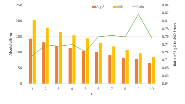
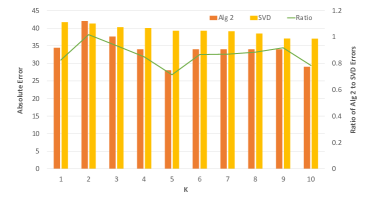
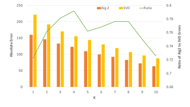
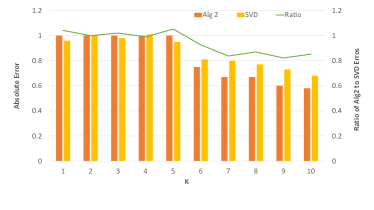
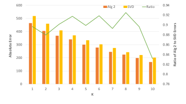
In this section, we show the effectiveness of Algorithm 2 compared to the SVD. We run our comparison both on synthetic as well as real data sets. For the real data sets, we use matrices from the FIDAP set and a word frequency dataset from UC Irvine . The FIDAP matrix is 27 $\times$ 27 with 279 real asymmetric non-zero entries. The KOS blog entries matrix, representing word frequencies in blogs, is 3430 $\times$ 6906 with 353160 non-zero entries. For the synthetic data sets, we use two matrices. For the first, we use a 20 $\times$ 30 random matrix with 184 non-zero entries—this random matrix was generated as follows: independently, we set each entry to $0$ with probability $0.7$, and to a uniformly random value in $[0,1]$ with probability $0.3$. Both matrices are full rank. For the second matrix, we use a random $\pm 1$ 20 $\times$ 30 matrix.

In all our experiments, we run a simplified version of Algorithm 2, where instead of running for all possible $\binom{[m]}{k}$ subsets of $k$ columns (which would be computationally prohibitive), we repeatedly sample $k$ columns, a few thousand times, uniformly at random. We then run the $\ell_{p}$-projection on each sampled set and finally select the solution with the smallest $\ell_{p}$-error. (While this may not guarantee provable approximations, we use this a reasonable heuristic that seems to work well in practice, without much computational overhead.) We focus on $p=1$ and $p=\infty$.

Figure 1 illustrates the relative performance of Algorithm 2 compared to the SVD for different values of $k$ on the real data sets. In the figure the green line is the ratio of the total error. The $\ell_{1}$-error for Algorithm 2 is always less than the corresponding error for the SVD and in fact consistently outperforms the SVD by roughly 40% for small values of $k$ on the FIDAP matrix. On the larger KOS matrix, the relative improvement in performance with respect to $\ell_{\infty}$-error is more uniform (around 10%).

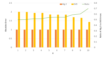
We observe similar trends for the synthetic data sets as well. Figures 2 and 3 illustrate the trends. Algorithm 2 performs consistently better than the SVD in the case of $\ell_{1}$-error for both the matrices. In the case of $\ell_{\infty}$-error, it outperforms SVD by around $10\%$ for higher values of $k$ on the random matrix. Furthermore, it consistently outperforms SVD, between 30% and 50%, for all values of $k$ on the random $\pm 1$ matrix.

To see why our $\ell_{\infty}$ error is always $1$ for a random $\pm 1$ matrix $A$, note that by setting our rank-$k$ approximation to be the zero matrix, we achieve an $\ell_{\infty}$ error of $1$. This is optimal for large values of $n$ and $m$ and small $k$ as can be seen by recalling the notion of the sign-rank of a matrix $A\in\{-1,1\}^{n\times m}$, which is the minimum rank of a matrix $B$ for which the sign of $B_{i,j}$ equals $A_{i,j}$ for all entries $i,j$. If the sign-rank of $A$ is larger than $k$, then for any rank-$k$ matrix $B$, we have $\|A-B\|_{\infty}\geq 1$ since necessarily there is an entry $A_{i,j}$ for which $|A_{i,j}-B_{i,j}|\geq 1$. It is known that the sign-rank of a random $m\times m$ matrix $A$, and thus also of a random $n\times m$ matrix $A$, is $\Omega(\sqrt{m})$ with high probability [8].

7 Conclusions

We studied the problem of low-rank approximation in the entrywise $\ell_{p}$ error norm and obtained the first provably good approximation algorithms for the problem that work for every $p\geq 1$. Our algorithms are extremely simple, which makes them practically appealing. We showed the effectiveness of our algorithms compared with the SVD on real and synthetic data sets. We obtain a $k^{O(1)}$ approximation factor for every $p$ for the column subset selection problem, and we showed an example matrix for this problem for which a $k^{\Omega(1)}$ approximation factor is necessary. It is unclear if better approximation factors are possible by designing algorithms that do not choose a subset of input columns to span the output low rank approximation. Resolving this would be an interesting and important research direction.

References

- [1] J.P. Brooks, J.H. Dulá, and E.L. Boone. A pure -norm principal component analysis. Computational Statistics & Data Analysis, 61:83–98, 2013.
- [2] Emmanuel J. Candès, Xiaodong Li, Yi Ma, and John Wright. Robust principal component analysis? JACM, 58(3):11:1–11:37, 2011.
- [3] C. Dan, K. A. Hansen, H. Jiang, L. Wang, and Y. Zhou. On low rank approximation of binary matrices. Technical Report 1511.01699v1, arXiv, 2015.
- [4] Anirban Dasgupta, Petros Drineas, Boulos Harb, Ravi Kumar, and Michael W. Mahoney. Sampling algorithms and coresets for regression. SICOMP, 38(5)(2060–2078), 2009.
- [5] Amit Deshpande, Madhur Tulsiani, and Nisheeth K. Vishnoi. Algorithms and hardness for subspace approximation. In SODA, pages 482–496, 2011.
- [6] A. Eriksson and A. van den Hengel. Efficient computation of robust low-rank matrix approximations using the norm. PAMI, 34(9):1681–1690, 2012.
- [7] Dan Feldman, Amos Fiat, Micha Sharir, and Danny Segev. Bi-criteria linear-time approximations for generalized -mean/median/center. In SoCG, pages 19–26, 2007.
- [8] Jürgen Forster. A linear lower bound on the unbounded error probabilistic communication complexity. J. Comput. Syst. Sci., 65(4):612–625, 2002.
- [9] Shmuel Friedland and Anatoli Torokhti. Generalized rank-constrained matrix approximations. SIAM Journal on Matrix Analysis and Applications, 29(2):656–659, 2007.
- [10] Nicolas Gillis and Stephen A. Vavasis. On the complexity of robust PCA and -norm low-rank matrix approximation. Technical Report 1509.09236, arXiv, 2015.
- [11] S. A. Goreinov and E. E. Tyrtyshnikov. The maximal-volume concept in approximation by low-rank matrices. Contemporary Mathematics, 208:47–51, 2001.
- [12] S. A. Goreinov and E. E. Tyrtyshnikov. Quasioptimality of skeleton approximation of a matrix in the Chebyshev norm. Doklady Mathematics, 83(3):374–375, 2011.
- [13] Peter J. Huber. Robust Statistics. John Wiley & Sons, New York,, 1981.
- [14] Qifa Ke and Takeo Kanade. Robust norm factorization in the presence of outliers and missing data by alternative convex programming. In CVPR, pages 739–746, 2005.
- [15] Cewu Lu, Jiaping Shi, and Jiaya Jia. Scalable adaptive robust dictionary learning. TIP, 23(2):837–847, 2014.
- [16] Deyu Meng and Fernando. D. L. Torre. Robust matrix factorization with unknown noise. In ICCV, pages 1337–1344, 2013.
- [17] Praneeth Netrapalli, U. N. Niranjan, Sujay Sanghavi, Animashree Anandkumar, and Prateek Jain. Non-convex robust PCA. In Advances in Neural Information Processing Systems 27: Annual Conference on Neural Information Processing Systems 2014, December 8-13 2014, Montreal, Quebec, Canada, pages 1107–1115, 2014.
- [18] Zhao Song, David P. Woodruff, and Pelin Zhong. Low rank approximation with entrywise -norm error. Technical Report 1611.00898, arXiv, 2016.
- [19] Naiyan Wang, Tiansheng Yao, Jingdong Wang, and Dit-Yan Yeung. A probabilistic approach to robust matrix factorization. In ECCV, pages 126–139, 2012.
- [20] Naiyan Wang and Dit-Yan Yeung. Bayesian robust matrix factorization for image and video processing. In ICCV, pages 1785–1792, 2013.
- [21] David P. Woodruff. Sketching as a tool for numerical linear algebra. Foundations and Trends in Theoretical Computer Science, 10(1-2):1–157, 2014.
- [22] L. Xiong, X. Chen, and J. Schneider. Direct robust matrix factorization for anomaly detection. In ICDM, pages 844–853, 2011.
- [23] H. Xu, C. Caramanis, and S. Sanghavi. Robust PCA via outlier pursuit. TOIT, 58(5):3047–3064, 2012.
- [24] L. Xu and A. L. Yuille. Robust principal component analysis by self-organizing rules based on statistical physics approach. IEEE Transactions on Neural Networks, 6(1):131–143, 1995.
- [25] Xinyang Yi, Dohyung Park, Yudong Chen, and Constantine Caramanis. Fast algorithms for robust pca via gradient descent. In D. D. Lee, M. Sugiyama, U. V. Luxburg, I. Guyon, and R. Garnett, editors, Advances in Neural Information Processing Systems 29, pages 4152–4160. Curran Associates, Inc., 2016.
- [26] Y. Zheng, G. Liu, S. Sugimoto, S. Yan, and M. Okutomi. Practical low-rank matrix approximation under robust -norm. In CVPR, pages 1410–1417, 2012.