Symmetric Gapped Interfaces of
SPT and SET States: Systematic Constructions
Juven Wang1
♯♯\sharp♯♯\sharpe-mail: juven@ias.edu,
Xiao-Gang Wen2
♮♮\natural♮♮\naturale-mail: xgwen@mit.edu
and Edward Witten1
♭♭\flat♭♭\flate-mail: witten@ias.edu
The arXiv:1705.06728 version is the original untrimmed version.
The Phys. Rev. X 8, 031048 (2018) published version is the trimmed version.
1School of Natural Sciences, Institute for Advanced Study, Einstein Drive, Princeton, NJ 08540, USA
2Department of Physics, Massachusetts Institute of Technology, Cambridge, MA 02139, USA
Symmetry protected topological (SPT) states have boundary ’t Hooft anomalies that obstruct an effective boundary theory realized in its own dimension with UV completion and with an on-site -symmetry. In this work, yet we show that a certain anomalous non-on-site symmetry along the boundary becomes on-site when viewed as an extended symmetry, via a suitable group extension . Namely, a non-perturbative global (gauge/gravitational) anomaly in becomes anomaly-free in .
This guides us to construct exactly soluble lattice path integral and Hamiltonian of symmetric gapped boundaries,
always existent for any SPT state in any spacetime dimension of any finite symmetry group, including on-site unitary and anti-unitary time-reversal symmetries. The resulting symmetric gapped boundary can be described either by an -symmetry extended boundary of bulk , or more naturally by a topological emergent -gauge theory with a global symmetry on a 3+1D bulk or above. The excitations on such a symmetric topologically ordered boundary can carry fractional quantum numbers of the symmetry , described by representations of . (Apply our approach to a 1+1D boundary of 2+1D bulk, we find that a deconfined gauge
boundary indeed has spontaneous symmetry breaking with long-range order. The deconfined symmetry-breaking phase crosses over smoothly to a confined phase without a phase transition.) In contrast to known gapped boundaries/interfaces obtained via symmetry breaking (either global symmetry breaking or Anderson-Higgs mechanism for gauge theory), our approach is based on symmetry extension. More generally, applying our approach to SPT states, topologically ordered gauge theories and symmetry enriched topologically ordered (SET) states, leads to generic boundaries/interfaces constructed with a mixture of symmetry breaking, symmetry extension, and dynamical gauging.
1 Introduction
After the realization that a spin-1/2 antiferromagnetic Heisenberg chain in 1+1 dimensions (1+1D) admits a gapless state [1, 2] that “nearly” breaks the spin rotation symmetry (i.e. it has “symmetry-breaking” spin correlation functions that decay algebraically), many physicists expected that spin chains with higher spin, having less quantum fluctuations, might also be gapless with algebraic long-range spin order. However, Haldane [3] first realized that antiferromagnetic Heisenberg spin chains in 1+1D with integer spins have a gapped disordered phase with short-range spin correlations. At first, it was thought that those states are trivial disordered states, like a product state of spin-0 objects. Later, it was discovered that they can have degenerate zero-energy modes at the ends of the chain [4], similar to the gapless edge states of quantum Hall systems. This discovery led to a suspicion that these gapped phases of antiferromagnetic integer spin chains might be topological phases.
Are Haldane phases topological or not topological? What kind of “topological” is it? That was the question. It turns out that only odd-integer-spin Haldane phases (each site with an odd-integer spin) are topological, while the even-integer-spin Haldane phases (each site with an even-integer spin) are really trivial (a trivial vacuum ground state like the product state formed by spin-0’s). The essence of nontrivial odd-integer-spin Haldane phases was obtained in LABEL:GW0931, based on a tensor network renormalization calculation [6], where simple fixed-point tensors characterizing quantum phases can be formulated. It was discovered that the spin-1 Haldane phase is characterized by a non-trivial fixed-point tensor – a corner-double-line tensor. The corner-double-line structure implies that the spin-1 Haldane phase is actually equivalent to a product state, once we remove its global symmetry. However LABEL:GW0931 showed that the corner-double-line tensor is robust against any local perturbations that preserve certain symmetries (namely, symmetry in the case of the integer spin chain), but it flows to the trivial fixed point tensor if we break the symmetry. This suggests that, in the presence of symmetry, even a simple product state can be non-trivial (i.e. , distinct from the product state of spin-0’s that has no corner-double-line structure), and such non-trivial symmetric product states were named Symmetry Protected Topological states (SPTs). (Despite its name, an SPT state has no intrinsic topological order in the sense defined in LABEL:W9039,CGW1038. By this definition, an SPT state with no topological order cannot be deformed into a trivial disordered gapped phase in a symmetry-preserving fashion.)
Since SPT states are equivalent to simple product states if we remove their global symmetry, one quickly obtained their classification in 1+1D [9, 10, 11], in terms of projective representations [12] of the symmetry group . As remarked above, one found that only the odd-integer-spin Haldane phases are non-trivial SPT states. The even-integer-spin Haldane phases are trivial gapped states, just like the disordered product state of spin-0’s [13]. Soon after their classification in 1+1D, bosonic SPT states in higher dimensions were also classified based on group cohomology and [14, 15, 16, 17], 111 For D SPT states (possibly with a continuous symmetry), here we use the Borel group cohomology or to classify them [14, 17]. Note that , where is the topological cohomology of the classifying space of . When is a finite group, we have only the torsion part . or based on cobordism theory [18, 19, 20]. In fact, SPT states and Dijkgraaf-Witten gauge theories [21] are closely related: Dynamically gauging the global symmetry [22, 23] in a bosonic SPT state leads to a corresponding Dijkgraaf-Witten bosonic topological gauge theory.
To summarize, SPT states are the simplest of symmetric phases and, accordingly, have another name Symmetry Protected Trivial states. They are quantum-disordered product states that do not break the symmetry of the Hamiltonian. Naively, one would expect that such disordered product states all have non-fractionalized bulk excitations. What is nontrivial about an SPT state is more apparent if one considers its possible boundaries. For any bulk gapped theory with symmetry, a -preserving boundary is described by some effective boundary theory with symmetry . However, the boundary theories of different SPT states have different ’t Hooft anomalies in the global symmetry [24, 25, 26, 27]. A simple explanation follows: While the bulk of SPT state of a symmetry group G has an onsite symmetry, the boundary theory of SPT state has an effective non-onsite G-symmetry. Non-onsite G-symmetry means that the G-symmetry does not act in terms of a tensor product structure on each site, namely the G-symmetry acts non-locally on several effective boundary sites. Non-onsite symmetry cannot be dynamically gauged — because conventionally the gauging process requires inserting gauge variables on the links between the local site variables of G-symmetry. Thus the boundary of SPT state of a symmetry G has an obstruction to gauging, as ’t Hooft anomaly obstruction to gauging a global symmetry [28]. Such an anomalous boundary is the essence of SPT states: Different boundary anomalies characterize different bulk SPT states. In fact, different SPT states classify gauge anomalies and mixed gauge-gravity anomalies in one lower dimension [25, 26, 27].222 Thus, more precisely, as explained above, different SPT states have different ’t Hooft anomalies on the boundary. In this article, when we say gauge anomalies and mixed gauge-gravity anomalies on the boundaries of SPT states, we mean the ’t Hooft anomalies of global symmetries or spacetime diffeomorphisms, coupling to non-dynamical background probed field or background probed gravity. So the gauge anomalies and mixed gauge-gravity anomalies (on boundaries of SPTs) mean to be the background gauge anomalies and mixed background gauge-gravity anomalies: Both the gauge fields and gravitational fields are background non-dynamical probes.
From the above discussion, we realize that to understand the physical properties of SPT states is to understand the physical consequence of anomalies in the global symmetry on the boundary of SPT states, somewhat as in work of ’t Hooft on gauge theory dynamics in particle physics [28]. For a 1+1D boundary, it was shown that the anomalous global symmetry makes the boundary gapless and/or symmetry breaking [14]. However, in higher dimensions, there is a third possibility: the boundary can be gapped, symmetry-preserving, and topologically ordered. (This third option is absent for a 1+1D boundary roughly because there is no bosonic topological order in that dimension.333 Here we mean that there is no intrinsic 1+1D topological order in bosonic systems, neither in its own dimension nor on the boundary of any 2+1D bulk short-range entangled state. (Namely, we may say that there is no 1+1D bosonic topological quantum field theory robust against any local perturbation.) However, the 1+1D boundary of a 2+1D bulk long-range entangled state may have an intrinsic topological order. Moreover, in contrast, in a fermionic system, there is a 1+1D fermionic chain [29] with an intrinsic fermionic topological order. ) Concrete examples of topologically ordered symmetric boundaries have been constructed in particular cases [30, 31, 32, 33, 34, 35, 36, 37, 38]. In this paper, we give a systematic construction that applies to any SPT state with any finite444The symmetries may be ordinary unitary symmetries, or may include anti-unitary time-reversal symmetries. symmetry group , for any boundary of bulk dimension or more. Namely, we show that symmetry-preserving gapped boundary states always exist for any D bosonic SPT state with a finite symmetry group when . We also study a few examples, but less systematically, when SPT states have continuous compact Lie groups , and we study their symmetry-preserving gapped boundaries, which may or may not exist.
Symmetry-breaking gives a straightforward way to construct gapped boundary states or interfaces, since SPT phases are completely trivial if one ignores the symmetry. For topological phases described by group cocycles of a group , the symmetry-breaking mechanism can be described as follows. It is based on breaking the to a subgroup , corresponding to an injective homomorphism as
| (1.1) |
Here must be such that the cohomology class in that characterizes the D SPT or SET state becomes trivial when pulled back (or equivalently restricted) to . The statement that the class is “trivial” does not mean that the relevant -cocycle is 1 if we restrict its argument from to , but that this cocycle becomes a coboundary when restricted to .
Our approach to constructing exactly soluble gapped boundaries does not involve symmetry breaking but what one might call symmetry extension:
| (1.2) |
Here we extend to a larger group , such that is its quotient group, is its normal subgroup, and is a surjective group homomorphism, more or less opposite to the injective homomorphism related to symmetry breaking (eqn. (1.1)). and must be such that the cohomology class in that characterizes the SPT or SET state becomes trivial when pulled back to . For any finite and any class in , we show that suitable choices of and always exist, when the bulk space dimension . Physically the gapped phases that we construct in this way have the property that boundary degrees of freedom transform under an symmetry. However, in condensed matter applications, one should usually555See Sec. 3.2 for an example in which it is natural in condensed matter physics to treat as a global symmetry. See also a more recent work Ref. [39] applying the idea to 1+1D bosonic/spin chains or fermionic chains. assume that the subgroup of is gauged, and then (in the SPT case) the global symmetry acting on the boundary is , just as in the bulk. So in that sense, when all is said and done the boundary states that we construct simply have the same global symmetry as the bulk, and the boundaries become topological since is gauged. For 2+1D (or higher dimensional) boundaries, such symmetry preserving topological boundaries may have excitations with fractional -symmetry quantum numbers. The fact that the boundary degrees of freedom are in representations of rather than actually describes such a charge fractionalization.
The idea behind this work was described in a somewhat abstract way in Sec. 3.3 of Ref.[40], and a similar idea was used in Ref.[41] in examples. In the present paper, we develop this idea in detail and in a down-to-earth way, with both spatial lattice Hamiltonians and spacetime lattice path integrals that are ultraviolet (UV) complete at the lattice high energy scale. We also construct a mixture combining the symmetry-breaking and symmetry-extension mechanisms.
We further expand our approach to construct anomalous gapped symmetry-preserving interfaces (i.e. domain walls) between bulk SPT states, topological orders (TO) and symmetry enriched topologically ordered states (SETs). 666We remark that our approach to constructing gapped boundaries may not be applicable to some invertible topological orders (iTO, or the invertible topological quantum field theory [TQFT]) protected by no global symmetry. However, the gapped boundaries of certain iTO can still be constructed via our approach: For example, the 4+1D iTO with a topological invariant has a boundary anomalous 3+1D gauge theory. Here is the -th Stiefel-Whitney class of a tangent bundle over spacetime . We will recap the terminology for the benefit of some readers. SPTs are short-range entangled (SRE) states, which can be deformed to a trivial product state under local unitary transformations at the cost of breaking some protected global symmetry. Examples of SPTs include topological insulators [42, 43, 44]. Topological orders are long-range entangled (LRE) states, which cannot be deformed to a trivial product state under local unitarity transformations even if breaking all global symmetries. SETs are topological orders – thus LRE states– but additionally have some global symmetry. Being long-range entangled, TOs and SETs have richer physics and mathematical structures than the short-range entangled SPTs. Examples of TOs and SETs include fractional quantum Hall states and quantum spin liquids [45]. In this work, for TOs and SETs, we mainly focus on those that can be described by Dijkgraaf-Witten twisted gauge theories, possibly extended with global symmetries. We comment on possible applications and generalizations to gapped interfaces of bosonic/fermionic topological states obtained from beyond-group cohomology and cobordism theories in Sec. 6-7.
1.1 Summary of physical results
In this article, we study a certain type of boundaries for -SPT states with a -symmetry. This type of boundary is obtained by adding new degrees of freedom along the boundary that transform as a representation of a properly extended symmetry group via a group extension with a finite . Such an -symmetry extended (or symmetry enhanced) boundary can be fully gapped with an -symmetry, but without any topological order on the boundary. The last column in Tables 1-4 describes such symmetry extension.
Moreover, there is another type of boundary, obtained by gauging the normal subgroup of . This type of boundary is described by a deconfined -gauge theory and has the same -symmetry as the bulk. We have constructed exactly soluble model to realize such type of boundaries for any SPT state with a finite group symmetry, and for some SPT states with a continuous group symmetry. Tables 1, 2, 3 and 4 summarize physical properties of this type of boundaries obtained from exactly soluble models for various -SPT states in various dimensions.
Symm. group End-point states : , Odd-integer AF Heisenberg spin chain 2-dim Rep()
Symm. group : D.4/5.2 , 2 D.9 D.10 4 : D.11 , 2 D.16 4 : D.14 , 2 D.21 2 D.21 2
For 1+1D SPT states, their degenerate end states are described by a representation of , called Rep. The Rep is also a projective representation of when is Abelian (see Table 1).
For a 2+1D SPT state, the boundary -gauge deconfined phase corresponds to a gapped spontaneously symmetry breaking boundary (breaking a part of -symmetry), which is described by an unbroken edge symmetry group (see Table 2). (However, if we consider this boundary as an H-symmetry extended 1+1D gapped boundary of the 2+1D bulk G-SPT state, then the boundary has no spontaneous symmetry breaking. The full H symmetry is preserved.)
For a 3+1D SPT state, the boundary -gauge deconfined phase corresponds to a gapped symmetry preserving topologically ordered boundary described by a gauge theory (see Table 3). Higher or arbitrary dimensional results are gathered in Table 4. Note that the -cocycle for a finite Abelian group with its type Roman numeral index follows the notation defined in Ref. [27].
Symm. group 4 D.8 4 D.8 4 Rep 4 4 4 : D.17 4 Rep : D.18 4 Rep : D.15 4 Rep
Symm. group 32 Rep
The symmetry preserving gapped boundary has topological excitations that carry fractional quantum numbers of the global symmetry . Such a symmetry fractionalization is actually described by Rep in our theory (see Table 3). In the following we will explain such a result.
-
1.
First of all, we know that the -gauge theory has gauge charges (point particles) carrying the representation, Rep(), of its gauge group . Each distinct representation Rep() labels distinct gauge-charged particle excitations.
-
2.
Second, if the -gauge theory has a global -symmetry, one may naively think that a gauge charged excitation can be labeled by a pair (Rep(), Rep()), a representation Rep() from the gauge group and a representation Rep() from the symmetry group . The label (Rep(), Rep()) is equivalent to Rep. If gauge charged excitations can be labeled by Rep, this will implies that the gauge charged excitations do not carry any fractionalized quantum number of the symmetry (i.e. no fractionalization of the symmetry ).
-
3.
However, for the boundary -gauge theory (e.g. the 2+1D surface) of -SPT state, the gauge charge excitations are in general labeled by Rep with , instead of Rep. is a “twisted” product of and , which is the so-called projective symmetry group (PSG) introduced in Ref. [46]. When a gauge charged excitation is described by Rep instead of Rep, it implies that the particle carries a fractional quantum number of global symmetry . We say there is a fractionalization of the symmetry .
-
4.
Continued from the previous remark, if the gauge group is or , then Rep is also called the projective representation of , named Proj.Rep(). Projective representation of also corresponds to a fractionalization of the symmetry .
-
5.
The quantum dimension (i.e. the internal degrees of freedom) of a gauge-charged excitation labeled by Rep is given by the dimension of the Rep: . For our gauge theoretic construction, because the Rep always has an integer dimension, thus the corresponding gauge charge always has an integer quantum dimension . More general topological order may have an anyon excitation that has a non-integer or irrational quantum dimension .
The first three rows in Table 3 are for the three 3+1D time-reversal SPT states. The first one is within group cohomology [16] , the second one is beyond group cohomology [30], and the third one the stacking of the previous two. The fourth rows in Table 3 describes three different boundaries of the same -SPT states (also known as bosonic topological insulator). Here we like to comment about the quantum number on the symmetry preserving topological boundary of those SPT states.
-
1.
When a particle carries the fundamental Rep(), it means that the particle is a Kramer doublet (since ). The -symmetry is related to where the time reversal square to , say . This corresponds to the first and the third rows in Table 3, where boundary excitations carry various representations of , including Kramers doublets.
-
2.
When a particle carries the fundamental Rep(), it means that the particle is a Kramer singlet (since ). The -symmetry is related to where the time reversal (i.e. the reflection) square to the identity. This corresponds to the second row in Table 3 which has no time-reversal symmetry fractionalization. But the boundary topological particles in the boundary -gauge theory are all fermions [30].
1.2 Notations and conventions
Our notations and conventions are partially summarized here. SPTs stands for Symmetry Protected Topological state, TOs stands for topologically ordered state, and SETs stands for Symmetric-Enriched Topologically ordered state. In addition, aSPT and aSET stand for the anomalous boundary version of an SPT or SET state. Also “TI,” “TSC,” and “TP” stand for topological insulator, topological superconductor and topological paramagnet respectively. We may append “B” in front of “TI,” “TSC” and “TP” as “BTI,” “BTSC” and “BTP” for their bosonic versions, where underlying UV systems contain only bosonic degrees of freedom. A proper theoretical framework for all these aforementioned states (SPTs, SETs, etc) is beyond the Ginzburg-Landau symmetry-breaking paradigm[47, 48].
When we refer to “symmetry,” we normally mean the global symmetry. The gauge symmetry should be viewed as a gauge redundancy but not a symmetry.
The boundary theories of SPTs have anomalies [25, 26, 27]. The possible boundary anomalies of SPTs include perturbative anomalies [49] and non-perturbative global anomalies [50, 51]. The obstruction of gauging the global symmetries (on the SPT boundary) is known as the ’t Hooft anomalies [28]. Although SPTs can have both perturbative and non-perturbative anomalies, our construction of symmetric gapped interfaces is only applicable to SPTs with boundary non-perturbative anomalies.777We note that there is a terminology clash between condensed matter and high energy/particle physics literature on “Adler-Bell-Jackiw (ABJ) anomaly [52, 53].” In condensed matter literature [25], the phrase “ABJ anomaly [52, 53]” refers to “perturbative” anomalies (with classes, captured by the free part of cohomology/cobordism groups), regardless of further distinctions (e.g. anomalies in dynamical gauge theory, or anomalies in global symmetry currents, etc.). In condensed matter terminology, the ABJ anomaly is captured by a 1-loop diagram that only involves a fermion Green’s function (with or without dynamical gauge fields). Thus, the 1-loop diagram can be viewed as a property of a free fermion system even without gauge field. On the other hand, in high energy/particle physics literature, the perturbative anomaly without dynamical gauge field captured by a 1-loop diagram is referred to as a perturbative ’t Hooft anomaly, instead of the ABJ anomaly. Here we attempt to use a neutral terminology to avoid any confusion.
We may use the long/short-range orders (LRO/SRO) to detect Ginzburg-Landau order parameters. In particular, the LRO captures the two-point correlation function decaying to a constant value at a large distance or power-law decaying, that detects the spontaneous symmetry breaking or the gapless phases.
On the other hand, we may use short/long-range entanglement (SRE/LRE) to describe the gapped quantum topological phases. LUT stands for local unitary transformation. A short-range entangled (SRE) state is a gapped state that can be smoothly deformed into a trivial product state by LUT without a phase transition (some global symmetries may be broken during the deformation). A long-range entangled (LRE) state is a gapped state that is not any SRE state, namely that cannot be smoothly deformed into a trivial product state by LUT without a phase transition (even by breaking all global symmetries during the deformation). What are examples of SRE and LRE states? SPTs are SRE states, which at low energy are closely related to invertible topological quantum field theories, with an additional condition that there is no perturbative or non-perturbative pure gravitational anomalies888 We note that the definitions of gravitational anomalies in [17, 54] and [18] are different. This leads to different opinions, between [17, 54] and [18], whether SPT states allow non-perturbative global gravitational anomalies or not along their boundaries, especially for SPT states with time reversal symmetries. on the boundary (e.g. for a 1+1D boundary, the chiral central charge , or the thermal Hall conductance vanishes ). TOs and SETs are LRE states.
The D means the dimensional spacetime. We may denote the D boundary of a D manifold as . We denote Borel group cohomology of a group with coefficients as for the -th cohomology group, which is equivalent to a topological cohomology of classifying space of as , regardless whether the is a continuous or a discrete finite group. The -cocycles are the elements of a cohomology group and satisfy a cocycle condition . The above statements are true for both continuous and discrete finite . When is a continuous group, we can either view the cocycle as a measurable function on which gives rise to Borel group cohomology, or alternatively, view the cocycle as continuous around a trivial but more generally may contain branch cuts. When is a finite group, we further have . The denotes the Bockstein homomorphism. GSD stands for ground state degeneracy, which counts the number of the lowest energy ground states (so called the zero energy modes).
In a -dimensional spacetime, we write for homogenous cocycles, and for homogenous cochains. We also write for inhomogeneous cocycles, and for inhomogeneous cochains. We write for homogenous cocycles or cochains with both global symmetry variables and gauge variables, and for inhomogeneous cocycles or cochains with both global symmetry variables and gauge variables. Homogeneous cochains/cocycles are suitable for SPTs and SETs that have global symmetries, while the inhomogeneous cochains/cocycles are suitable for TOs that have only gauge symmetries with no global symmetries. The is the th Chern class and the is the th Stiefel-Whitney (SW) class. We generically denote the cyclic group of order as , but we write when we are referring to the distinct classes in a classification of topological phases or in a cohomology/bordism group. When convenient, we use notation such as , and to identify a particular copy of . We denote for the imaginary number where .
1.3 The plan of the article
We aim to introduce a systematic construction of various gapped boundaries/interfaces for bulk topological states based on the group extension. We had mentioned many examples with various bulk SPT states and different boundary states in any dimension, in Table 1 (1+1D bulk/0+1D boundary), Table 2 (2+1D bulk/1+1D boundary), Table 3 and Table 4 (3+1D bulk/2+1D boundary and higher dimensions). Their properties are summarized in Table 5 (for a finite discrete symmetry group ) and Table 6 (for a continuous symmetry group ), and their constructions are summarized in Table 7 . Furthermore, we can formulate more general gapped interfaces including not only our proposal on symmetry-extension, but also symmetry-breaking and dynamically gauging of topological states, in a framework, schematically shown in Table 8. We will provide both the spacetime lattice path integral (partition function) definition and the wavefunction (as a solution to a spatial lattice Hamiltonian) definition, see Table 9, for our generic construction.
We begin in Sec. 2, by reviewing a model that realizes the 2+1D SPT state, the CZX model. Then in Sec. 3, we construct various boundaries, both gapless and gapped, for the CZX model. In the process, we illustrate some of the main ideas of this paper. In Appendix A, we examine various low-energy effective theories for the boundaries of CZX model. Among the new phenomena, we find that in Appendix A.2.4 the 1+1D boundary deconfined and confined -gauge states belong to the same phase, namely they are both spontaneous symmetry breaking states related by a crossover without phase transition. In Appendix B, we study the fermionic version of CZX model, then we find anomalous boundary with emergent -gauge theory and anomalous global symmetry in Appendix C. We expect that our approach can apply to other generic fundamentally fermionic many-body systems.
All these analyses have the advantage of illustrating our constructions in a completely explicit way, but they have a drawback. The deconfined gapped boundary state that we construct for the CZX model (in the usual case that the global symmetry is not extended along the boundary) is not really a fundamentally new state with 1+1D topological order, but rather it can be interpreted in terms of broken global symmetry.999 More generally, we find that, various 1+1D deconfined gauge theories (on the boundaries of 2+1D SPT states) are the spontaneous global symmetry breaking states with either unitary-symmetry or anti-unitary time reversal -symmetry broken, see Sec. 4.8 and Appendices A.2.4 and D.22. This is consistent with the common lore that “there is no true topological order in 1+1D that is robust against any local perturbation.” However, we start with the CZX model because in that case everything can be stated in a particularly simple and clear way. Models in higher dimension ultimately realize the ideas of the present paper in a more satisfying way – as the phases we construct are essentially new – but in higher dimension, it is hard to be equally simple.
Nevertheless, the extrapolation from our detailed treatment of the CZX model to a general discussion in higher dimensions is fairly clear. In Sec. 4, we distill the essence of the non-on-site boundary symmetry of a generic SPT state in any dimension. One key message of this section is the following: The symmetry-extended gapped boundary construction of a bulk -SPTs relies on the fact that its boundary has a non-perturbative global -anomaly (probed by gauge or gravitational fields, as a non-perturbative global gauge/gravitational anomalies) which becomes an -anomaly-free by pulling back to .
In Sec. 4.7.1, we introduce the concept of “soft gauge theory” and introduce the cochains that encode the soft gauge degree of freedom. We consider an emergent soft gauge theory on the boundary, associated to a suitable group extension as eqn. (1.2), as a way to construct a symmetric gapped boundary state. (The “soft gauge theory” and the usual “hard gauge theory” are contrasted later in Sec. 9.) In Sec. 5, we provide a method, in the context of an arbitrary SPT phase with symmetry , to search for an -extension of that trivializes the -cocycle. We provide valid examples of symmetric gapped boundaries for SPTs with onsite unitary symmetry (Sec. 5.2) and anti-unitary time reversal symmetry (Sec. 5.3) in 2+1D and 3+1D, more examples for any dimensions are given in Appendix D.
In Sec. 6 and Sec. 7, we comment on the application of our approach for gapped interfaces of topological states obtained from beyond-symmetry-group cohomology and cobordism approach, for both bosonic and fermionic systems.
In Sec. 8, we consider generic gapped boundaries and gapped interfaces (Sec. 8.3) with mixed symmetry-breaking (Sec. 8.1 and Appendix E), symmetry-extension and dynamically-gauging mechanisms (Sec. 8.2). Dynamically gauged gapped interfaces of topologically ordered gauge theories are explored in Sec. F (more examples are relegated to Appendix F.1).
We also describe two different techniques to obtain symmetry-extended gapped boundaries / interfaces. One technique is in Sec. 5: For a given symmetry (quotient) group and its -cocycle, we can determine the finite (normal subgroup) and then deduce the total group , in order to obtain the trivialization of -topological state via the exact sequence in eqn. (1.2). Another technique in Appendix D.3 is based on Lydon-Hochschild-Serre (LHS) spectral sequence method. Given the symmetry group and its -cocycle, and suppose we assume the possible and within , the LHS method helps to construct an exact analytic function of the split -cochain from the given -cocycle and from the exact sequence eqn. (1.2). In short, both techniques have their own strengths: The first technique in Sec. 5 has the advantage to search and , for a given and a -cocycle, The second LHS’s technique in Appendix D.3 has the further advantage to construct the exact analytic split -cochain.
In Sec. 9, we provide a systematic general construction of lattice path integrals and Hamiltonians for gapped boundaries/interfaces for topological phases in any dimension. More examples of symmetry-extended gapped interfaces in various dimensions are provided in Appendix D. Many examples of gauge symmetry-breaking gapped boundaries/interfaces via Anderson-Higgs mechanism are derived based on our framework, and compared to the previous known results in the literature, in Appendix F.1. We conclude in Sec. 10.
1.4 Tables as the guide to the article
Readers can either find the following Tables 5, 6, 7, 8 and 9 and Fig. 1 as a quick tabular summary of partial results of the article, or find them as a useful guide or menu to the later Sections. Readers may freely skip the entire Sec. 1.4 and Tables, then proceed to Sec. 2 directly, and come back to these Tables later after visiting related materials in the later Sections.

In Table 5 and 6, we discuss various boundary properties of a finite group symmetry -SPTs (Table 5) and a continuous group symmetry -SPTs (Table 6). The discussions here parallel to the topological phase constructions in Table 7 and 8, and we enumerate the items in the similar orderings shown there.
A schematic physical picture is shown in Fig. 1. Conceptually, we could ask how a phase diagram of the Hamiltonian’s coupling space in a symmetry (the left figure of Fig. 1) evolves if we consider the phase diagram of the Hamiltonian’s coupling space in a larger symmetry (the left figure of Fig. 1). The effective Hilbert space for the whole system in the -symmetry may be larger than that in the -symmetry. Thus one may need to modify Hamiltonians as well as Hilbert spaces to consider such a phase-diagram evolution, which is difficult in practice. But as a thought experiment, we could expect that several distinct SPT states in may become the same trivial insulator/vacuum in . Those -SPT states contain certain non-perturbative global -anomalies along physical boundaries, that become anomaly-free in . We note that the phase boundaries in the phase diagrams shown in Fig. 1 are schematic only and are not equivalent to the physical boundaries to a trivial vacuum in the spacetime.
In Table 7 and 8, we show various gapped boundaries (bdry) and interfaces of topological states in -dimensional spacetime with their interfaces in -dimensions:
In Table 7 (i), -SPTs has an anomalous boundary with an anomalous non-onsite symmetry in (Sec. 4.3). However, the non-onsite -symmetry can be made to be onsite in , thus the -anomaly becomes anomaly free (denoted as anom. free) in (Sec. 4.5). This also gives us a way to obtain a -symmetry-extended gapped boundary of -SPTs.
In Table 7 (ii), -SPT state’s above boundary in (i) can be dynamically gauged on its normal subgroup on the boundary. We denote such a boundary state as -aSETs, which means that it has a full group , a dynamical gauge group , and with a -anomaly.
Symmetry extension construction: , with and finite groups. A -topological state (e.g. -cocycle or bundle) is trivialized in . For a bulk -SPTs, its boundary has a non-perturbative global -anomaly from (for a finite , containing only the torsion), which becomes an -anomaly free by pulling back to . Formally, we can prove that, given a -cocycle , certain finite and exist, so , split to -cochains . The bulk+boundary theory has an on-site -symmetry. The effective boundary theory has a local Hilbert space, but has a non-on-site -symmetry (4.3.2). The bulk+boundary theory has an on-site symmetry. The effective boundary theory has a local Hilbert space, and has an on-site -symmetry (4.4.2). The boundary -anomaly becomes -anomaly free (4.4.2). Interpretation: (i) Extending to -symmetry only on the boundary, but the model is artificial in condensed matter (3.2, D.23). (ii) A nontrivial bulk -SPTs becomes a trivial bulk -SPTs (trivial vacuum), when pulling back to (4.3.2). The effective boundary theory has a non-local Hilbert space, therefore its on-site or non-on-site symmetry is ill-defined (4.6.2). For 2+1D bulk/1+1D boundary, a deconfined boundary -gauge theory has a spontaneous symmetry breaking (SSB) long-range order in , either breaking unitary (e.g. ) or anti-unitary time reversal (Sec. 3.3, A.2.4, D.22) subgroup in . The SSB states smoothly cross over to confined states. We find no robust intrinsic topological order even on a 1+1D boundary of SPTs. For 3+1D bulk/2+1D boundary or higher dimensions, there always exists a symmetry-preserving deconfined boundary -gauge theory with a robust intrinsic topological order. The -gauge charge carries a representation Rep(). The -anomaly is a non-perturbative global (gauge/gravitational) anomaly that becomes absence in . Given a finite , we can find a finite Abelian to achieve this (Sec. 5). The bulk+boundary theory has an on-site symmetry. The effective boundary theory has a local Hilbert space, but has a non-on-site -symmetry (4.7.2). The effective boundary theory has a non-local Hilbert space, which cannot be local even by soft-gauging, therefore its on-site or non-on-site symmetry is ill-defined (for SETs). This relates to the fact that an intrinsic bulk topological order has long-range entanglements and gravitational anomaly.
Symmetry extension construction: , with and as continuous groups (in particular compact Lie groups) but as a finite group. The finite group extension from a continuous to a continuous by a finite is the finite covering of . For a bulk -SPTs (classified by ), its boundary may either have a perturbative -anomaly from the free part of (e.g. a perturbative anomaly with a class), or a non-perturbative global -anomaly from the torsion part of (e.g. global anomaly with a product of classes). Only a non-perturbative global -anomaly from the torsion part may become -anomaly free. Similarly, only the corresponding -SPTs may be trivialized in . Our approach suggests a method to find a continuous to construct symmetry-preserving gapped boundaries: either an -symmetry extended gapped boundary, or a deconfined finite -gauge theory, for such as a -SPTs. For 2+1D bulk/1+1D boundary, if a deconfined boundary -gauge theory exists, it has a spontaneous symmetry breaking long-range order in , either breaking unitary (e.g. in Sec. 3.3, A.2.4, D.22) or anti-unitary time reversal discrete finite subgroup in the full . We find no spontaneous global symmetry breaking for the continuous subgroup sector in on the 1+1D boundary, consistent with Coleman-Mermin-Wagner theorem. We also find no robust intrinsic topological order on a 1+1D boundary of SPTs. (e.g. and in D.22) For 3+1D bulk/2+1D boundary or higher dimensions, there may or may not exist a symmetry-preserving deconfined boundary -gauge theory. Our construction depends on the properties of continuous and : - - - - - - - - - - - - - - - - - - - - - - - - - - - - - - - - - - - - - - - - - - - - - - - - - - - - - - - - When a continuous Lie group is connected but not simply-connected, there exists a finite extension of as a finite covering of from (e.g. ). When is disconnected, there may still exist a finite covering (e.g. ). Two scenarios: If -anomaly is a perturbative anomaly, then the group extension of to cannot make this -anomaly free. There exists no boundary deconfined gauge theory with topological orders for such a -SPTs. (e.g. D.19’s chiral anomaly.) If -anomaly is a non-perturbative global anomaly, we can check whether the group extension of to , by a finite , makes it -anomaly free. If yes, then deconfined- gauge theories exist with robust intrinsic topological orders. For examples, D.20’s -global anomaly, D.8’s -BTSC with , or 3+1D -BTP (shown in Table 3), which finite coverings are allowed from or . - - - - - - - - - - - - - - - - - - - - - - - - - - - - - - - - - - - - - - - - - - - - - - - - - - - - - - - - When a continuous Lie group is simply-connected, then there is no finite extension of because there is no finite covering of . (e.g. for .) Thus our construction fails to construct symmetry-preserving gapped boundary of such a -SPTs. This implies either that boundary states must be symmetry-enforced gapless, or one needs to seek other construction (different from ours) for symmetry-preserving gapped boundary. The properties of global symmetry (on-site or non-on-site) for continuous and still follow the similar discussions as in Table 5.
(i) (ii) (iii) (iv) (v) (vi)
(vii)
| Dim | Spacetime lattice (for path integral ) | Spatial lattice (for Hamiltonian ) |
| 1+1D |
1+1D |
… |
| 2+1D |
2+1D ![[Uncaptioned image]](/html/1705.06728/assets/x10.png)
|
2D |
| 3+1D | … |
3D ![[Uncaptioned image]](/html/1705.06728/assets/x12.png)
|
| … | … | … |
In Table 7 (iii), -gauge means a generic twisted -gauge theory (possibly with a Dijkgraaf-Witten cocycle). The -aGauge on the boundary means that it has a full dynamical gauge group on the boundary. But the boundary theory is not the usual gauge theory in its own dimensions described by -cocycles, but by special -cochains with additional gauge holonomy conservation constraints.
In Table 7 (iv), -SETs means a SET state with a full group , a dynamical gauge group , and a global symmetry . The -aSETs means a symmetry-enriched boundary state with a full group , a dynamical gauge group and it has a boundary -anomaly (from anomalous non-onsite -global symmetry transformation on the boundary).
In Table 7 (v), - and -SPTs with non-onsite - and - symmetries can have an onsite -symmetry on the shared gapped interface.
Thus the two topological states become anomaly free by pulling them back to a certain larger .
In Table 7 (vi), the -SETs means a SET state with a full group , a dynamical gauge group , and individually has a global symmetry . The -SETs means a SET state with a full group , a dynamical gauge group , and individually has a global symmetry . A global symmetry on the whole system including the left and right sectors become . The aSETs means a symmetry-enriched boundary state, with a full group , a dynamical gauge group . The boundary has a -anomaly, where (from an anomalous non-onsite -global symmetry transformation on the boundary).
In Table 8 (vii), we consider generic topological state and topological state (of SPTs, TOs or SETs), and construct generic gapped interfaces based on mixed mechanisms of symmetry-extension, symmetry-breaking and dynamically gauging. The interface of is found by trivializing the nontrivial cocycle or bundle associated to via pulling back to from a generic group homomorphism .
2 A model that realizes the 2+1D SPT state: CZX model
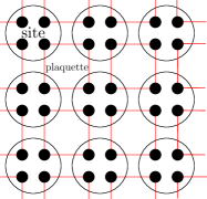
The first lattice model that realizes a 2+1D SPT state (the -SPT state) was introduced by Chen-Liu-Wen [14], and was named the CZX model. The CZX model is a model on a square lattice (Fig. 2), where each lattice site contains four qubits, or objects of spin-1/2. For each spin, we use a basis and of eigenstates. Thus a single site has a Hilbert space of dimension .
Now let us introduce a symmetry transformation. An obvious choice is the operator that acts on each site as
| (2.1) |
which simply flips the four spins in site . However, to construct the CZX model, a more subtle choice is made. In this model, in the basis , , the flip operator is modified with signs. For a pair of spins , we define an operator101010The name is read “controlled ” and is suggested by quantum computer science. The operator measures of spin if spin is in state and otherwise does nothing. that acts as if spins are both in state , and otherwise acts as . There are various ways to describe by a formula:
| (2.2) |
Now for a site that contains four spins in cyclic order, we define
| (2.3) |
The symmetry of the spins at site is defined as
| (2.4) |
By a short exercise, one can verify that and commute and accordingly that . The symmetry generator of the CZX model is defined as a product over all sites of :
| (2.5) |
Clearly this is an on-site symmetry, that is, it acts separately on the Hilbert space associated to each site. Being onsite, the symmetry is gaugeable and anomaly-free. We have not yet picked a Hamiltonian for the CZX model, but whatever -invariant Hamiltonian we pick, the symmetry can be gauged by coupling to a lattice gauge field that will live on links that connect neighboring sites.
What we have done so far is trivial in the sense that, by a change of basis on each site, we could have put in a more standard form. However this would complicate the description of the Hamiltonian and ground state wavefunction of the CZX model, which we come to next.
It is easier to first describe the desired ground state wavefunction of the model and then describe a Hamiltonian that has that ground state. In Fig. 2, we have drawn squares that contain four spins, one from each of four neighboring sites. We call these squares “plaquettes.” For each plaquette , we define the wavefunction . The ground state of the CZX model in the bulk is given by a product over all plaquettes of this wavefunction for each plaquette:
| (2.6) |
This state is -invariant,
| (2.7) |
if we define the whole system on a torus without boundary (i.e., with periodic boundary conditions). But that fact is not completely trivial: It depends on cancellations among factors for adjacent pairs of spins, see Fig. 3.
Clearly, the entanglement in this wavefunction is short-range, and this wavefunction describes a gapped state. Moreover, if we would regard the plaquettes (rather than the large discs in Fig. 2) as “sites,” then this wavefunction would be a trivial product state. But in that case the symmetry of the model would not be on-site. The subtlety of the model comes from the fact that we cannot simultaneously view it as a model with on-site symmetry and a model with a trivial product ground state.
(1)  (2)
(2) 
The most obvious Hamiltonian with as its ground state would be a sum over all plaquettes of an operator that flips all spins in plaquette :
| (2.8) |
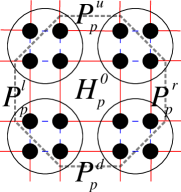
This Hamiltonian commutes with the obvious symmetry that flips all the spins, but does not commute with the more subtle symmetry . To commute with , we modify to only flip the spins in a plaquette if adjacent pairs of spins in the neighboring plaquettes are equal (Fig. 3). For a plaquette , we define operators that project onto states in which the two spins adjacent to in the direction (where equals up, down, left, or right, denoted as , , , or ) are equal. Then the CZX Hamiltonian is defined to be
| (2.9) |
Thus each acts on the spins contained in an octagon (Fig. 4(1)), flipping the spins in a plaquette if all adjacent pairs of spins are equal. This Hamiltonian is -invariant,
| (2.10) |
in the case of a system without boundary (an infinite system or a finite system with periodic boundary conditions). The state is a symmetry-preserving ground state with short-range entanglement. However, it is a nontrivial symmetry-protected topological or SPT state. This becomes clear if we examine possible boundaries of the CZX model.
3 Boundaries of the CZX model
3.1 The first boundary of the CZX model –
1+1D symmetry-preserving gapless boundary
with a non-on-site global -symmetry
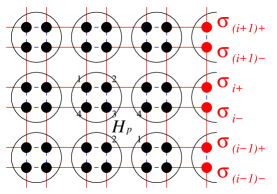
The boundary of the CZX model that was studied in the original paper is a very natural one in which one simply considers a finite system with an integer number of sites (Fig. 4(2)). One groups the spins into plaquettes, as before, but as shown in the figure, there is a row of spins on the boundary that are not contained in any complete plaquette. We call these the boundary spins.
We define the Hamiltonian as in eqn. (2), where now the sum runs over complete plaquettes only. Because the boundary spins are not contained in any complete plaquette, the system is no longer gapped. However, the boundary spins are not completely free to fluctuate at no cost in energy. The reason is that, to minimize the energy, a pair of boundary spins that are adjacent to a plaquette are constrained to be equal. This is because of the projection operators in the definition of .
Hence, in a state of minimum energy, the boundary spins are locked together in pairs. These pairs are denoted as , , etc., in Fig. 4(2), and one can think of them as composite spins.
How does the symmetry generated by act on the composite spins? Evidently, will flip each composite spin. However, also acts by a operation on each adjacent pair of composite spins , . That is because, for example, in Fig. 4(2), the “upper” spin making up the composite spin and the “lower” spin making up are adjacent spins contained in the same site in the underlying square lattice. Accordingly, in the generator for site , there is a factor linking these two spins.
Therefore, the effective generator for the composite spins on the boundary is
| (3.1) |
The product runs over all composite spins ; is the product of operators that flip and operators that give the usual sign factors for each successive pair of composite spins. Clearly, this effective symmetry is not on-site. No matter how we group a finite set of composite spins into boundary sites, the operator will always contain factors linking one site to the next.111111In the case of a compact ring boundary, for an even-site boundary, while for an odd-site boundary. To avoid the even or odd lattice site effect, from now on we assume the even-site boundary system throughout our work for simplicity. If there are no corners or spatial defects or curvature – which would lead to corrections in these statements – then the number of odd-site boundary components is always even, so overall .
With the Hamiltonian as we have described it so far, all states labeled by any values of the composite spins , but with complete bulk plaquettes placed in their ground state , are degenerate. Of course, it is possible to add perturbations that partly lift the degeneracy. However, it has been shown in Ref.[14] that the non-onsite nature of the effective symmetry gives an obstruction to making the boundary gapped and symmetry-preserving.
3.2 The second boundary of the CZX model –
1+1D gapped boundary by
extending the -symmetry to a -symmetry
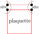
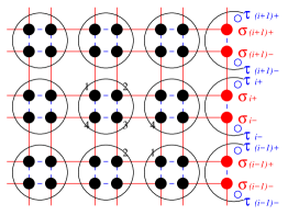
The main idea of the present paper can be illustrated by a simple alternative boundary of the CZX model. To construct this boundary, we simply omit the boundary spins from the previous discussion. This means that now, the system is made of complete plaquettes, even along the boundary (Fig. 5), but there is a row of boundary spins that are not in complete sites. As indicated in the figure, we combine the boundary spins in pairs into boundary sites. Thus a boundary site has only two spins while a bulk site has four. In the figure, we have denoted the “upper” and “lower” spins in the boundary site as and .
To specify the model, we should specify what the Hamiltonian looks like near the boundary and how the global symmetry is defined for the boundary spins. First of all, now that all spins are in complete plaquettes, we can look for a gapped system with the same ground state wave function as in eqn. 2.6:
| (3.2) |
To get this ground state, we define the Hamiltonian by the same formula as in eqn. (2). Only one very small change is required: A boundary plaquette is adjacent to only three pairs of spins instead of four, so in the definition of in eqn. (2), if is a boundary plaquette, the product of projection operators contains only three factors and not four.
The last step is to define the action of the global “” symmetry for boundary sites. We have put “” in quotes for a reason that will be clear in a moment. Once we have chosen the Hamiltonian as above, the choice of the global symmetry generator is forced on us. The symmetry generator at the boundary site will have to flip the two spins and , of course, but it also needs to have a factor linking these two spins. So the symmetry generator of the boundary site will have to be
| (3.3) |
The full symmetry generator is
| (3.4) |
where the product runs over all bulk or boundary sites , and is defined in the usual way for bulk sites, and as in eqn. (3.3) for boundary states.
We have found a gapped, symmetry-preserving boundary state for the CZX model. There is a catch, however. The global symmetry is no longer . Although the operator squares to 1 if is a bulk site, this is not so for boundary sites. Rather, from (3.3), we find that for a boundary site,
| (3.5) |
This operator is if the two spins and in the boundary site are both up or both down, and otherwise . Clearly , so the full global symmetry generator does not obey but rather
| (3.6) |
Thus, rather than the symmetry being broken by our choice of boundary state, it has been enhanced from to . But a subgroup of generated by acts only on the boundary, since for bulk sites.
What we have here is a group extension
| (3.7) |
is the global symmetry group of the bulk theory, is the global symmetry of the complete system including its boundary, and (or a different ) is the subgroup of that acts only along the boundary. In this case, we denote the exact sequence eqn.(3.7) also as
As was explained from an abstract point of view in Sec. 3.3 of Ref.[40] and as we will explain more concretely later in this paper, when certain conditions are satisfied, such a group extension along the boundary gives a way to construct gapped boundary states of a bulk SPT phase. (As we explain in detail later, the relevant condition is that the cohomology class of that characterizes the SPT state in question should become trivial if it is “lifted” or “pulled back” from to , or more concretely if certain fields are regarded as elements of rather than as elements of .)
From a mathematical point of view, this gives another choice in the usual paradigm that says that the boundary of an SPT phase either is gapless, has topological order on the boundary, or breaks the symmetry. Another possibility is that the global symmetry of the bulk SPT phase might be extended (or enhanced) to a larger group along the boundary, satisfying certain conditions. In dimensions, this is a standard result: The usual symmetry-preserving boundaries of -dimensional bulk SPT phases have a group extension along the boundary. The novelty is that a gapped boundary can be achieved above dimensions via such a group extension.
Let us pause to explain more fully the assertion that what we have just described extends a standard -dimensional phenomenon to higher dimensions. In the usual formulation of the -dimensional Haldane or Affleck-Lieb-Kennedy-Tasaki (AKLT) spin chain, one considers a chain of spin 1 particles with symmetry. The boundary is not gapped and carries spin 1/2. Alternatively, one could attach a spin 1/2 particle to each end of such a chain. Then the system can be gapped, with a unique ground state, but the global symmetry is extended from to at the ends of the chain. What we have described is an analog of such symmetry extension in dimensions.
In general, a bulk SPT state protected by a symmetry , can also be viewed as a many-body state with a symmetry , where the subgroup acts trivially in the bulk (i.e. the bulk degrees of freedom are singlets of ). For example, we may view the CZX model to have a symmetry in the bulk. By definition, two states in two different -SPT phases cannot smoothly deform into each other via deformation paths that preserve the -symmetry. However, two such -SPT states may be able to smoothly deform into each other if we view them as systems with the extended -symmetry and deform them along the paths that preserve the -symmetry. For example, the non-trivial -SPT state of the CZX model can smoothly deform into the trivial -SPT state along a deformation path that preserves the extended -symmetry. In other words, when viewed as a symmetric state, the ground state of the CZX model has a trivial -SPT order. Since it has a trivial -SPT order, it is not surprising that the CZX model can have a gapped boundary that preserves the extended symmetry, as explicitly constructed above. In general, if two -SPT states are connected by an -symmetric deformation path, then we can always construct a -symmetric domain wall between them by simply using the -symmetric deformation path. This is the physical meaning behind a -SPT state having a gapped boundary with an extended symmetry .
From the point of view of condensed matter physics, however, the sort of gapped boundary that we have described so far will generally not be physically sensible. Microscopically, condensed matter systems generally do not have extra symmetries that act only along their boundary. (There can be exceptions like the case just mentioned, which is conceivable in any dimension: a system that, in bulk, is made from particles of integer spin but has half-integer spin particles attached on the surface. Then a rotation of the spins is nontrivial only along the boundary.)
In a system microscopically without an extended symmetry along the boundary, one might be tempted to interpret as a group of emergent global symmetries, not present microscopically. But there is a problem with this. In condensed matter physics, one may often run into emergent global symmetries in a low-energy description. But these are always approximate symmetries, explicitly broken by operators that are irrelevant at low energies in the renormalization group sense.
That is not viable in the present context. Since the global symmetry that is generated by is supposed to be an exact symmetry, we cannot explicitly violate the boundary symmetry group generated by . Obviously, any interaction that is not invariant under is also not invariant under .
What we can do instead is to gauge the boundary symmetry group . Then, the global symmetry group that acts on gauge-invariant operators and on physical states is just the original group . This way, we do not break nor extend the symmetry on the boundary. Since is an on-site symmetry group, there is no difficulty in gauging it; we explain two approaches in Sec. 3.3 and 3.4.
In (or more) dimensions, a procedure along these lines starting with a bulk SPT phase with symmetry group and a group extension as in eqn. (3.7) that satisfies the appropriate cohomological condition will lead to a gapped boundary state with topological order along the boundary. The topological order is a version of gauge theory with gauge group (possibly twisted by a cocycle). We will give a general description of such gapped boundary states in Sec. 9. In dimensions, the boundary has dimension and one runs into the fact that topological order is not possible in dimensions. As a result, what we will actually get in the CZX model by gauging the boundary symmetry is not really a fundamentally new boundary state.
3.3 The third boundary of the CZX model – Lattice -gauge theory on the boundary

We will describe two ways to gauge the boundary symmetry . The most straightforward way, although as we will discuss ultimately less satisfactory for condensed matter physics, is to simply incorporate a boundary gauge field.
As indicated in Fig. 6, we label the link between boundary sites and by the half-integer . Placing a -valued gauge field on this link means introducing a qubit associated to this link with operators , that obey
| (3.8) |
Here describes parallel transport between sites and and is a discrete electric field that flips the sign of .
Now let us discuss the gauge constraint at site . A gauge transformation that acts at site by the nontrivial element in is supposed to flip the signs of , the holonomies on the two links connecting to site . To do this, it will have a factor . It should also act on the spins as . Thus the gauge generator on site is
| (3.9) |
A physical state in the gauge theory must be gauge-invariant, that is, it must obey
| (3.10) |
However, as for all , if we take the product of over all boundary sites, the factors of cancel out, and we get
| (3.11) |
Hence eqn. (3.10) implies that a physical state satisfies
| (3.12) |
But this precisely means that a physical state is invariant under the global action of , so that the global symmetry group that acts on the system reduces to the original global symmetry .
The Hamiltonian must be slightly modified to be gauge-invariant, that is, to commute with . To see the necessary modification, let us look at the plaquette Hamiltonian for the boundary plaquette shown in the figure, which contains the boundary link labeled . as defined in eqn. (2) anticommutes with and because the operator has that property. (It flips one of the spins at boundary site and one at boundary site , so it anticommutes with and similarly with .) To restore gauge-invariance is surprisingly simple: We just have to multiply by , which also anticommutes with and . So we can take the Hamiltonian for a boundary plaquette containing the boundary link to be
| (3.13) |
For a gauge-invariant and -invariant Hamiltonian, we can take the sum of all bulk and boundary plaquette Hamiltonians.
This Hamiltonian commutes with all the discrete gauge fields , so in looking for an eigenstate of (ignoring for a moment the gauge constraint), we can specify arbitrarily the eigenvalues of the ’s. Let be a state of the gauge fields with eigenvalue for . (Of course these eigenvalues are since .) The ground state of with these eigenvalues of the is simply
| (3.14) |
Let us denote this state as . If the boundary has links, there are of these states.
The states are degenerate, and these are the ground states of . However, to make states that satisfy the gauge constraint, we must take linear combinations of the . Since a gauge transformation at site flips the signs of , the only gauge-invariant function of the is their product. Assuming that the boundary is compact and thus is a circle, this product is the holonomy of the gauge field around the circle. (With periodic boundary conditions along the boundary, there are no corners along the boundary circle; otherwise, our discussion can be slightly modified to incorporate corners.) Thus there are two gauge-invariant ground states, depending on the sign of the holonomy . They are
| (3.15) |
and
| (3.16) |
(Here the signs are determined by the gauge constraints. With our choice of sign in the gauge constraints , flipping two of the that are separated by lattice states multiplies the amplitude by . This could be avoided by changing the sign of , but that creates complications elsewhere.)
Now let us study the transformation of these states under the global symmetry group . When we apply to the states , we find that all the sign factors cancel each other. This occurs by the same cancellation as in the original bulk version of the CZX model. However, the wavefunction is no longer trivially invariant under flipping the spins; rather, the wavefunction for a boundary plaquette is multiplied by when the spins in this plaquette are flipped. So taking into account all the boundary plaquettes,
| (3.17) |
Thus, the transformation of a state under the global symmetry is locked to its holonomy under the gauge symmetry .
The formula (3.17) has been written as if the boundary of the system consists of a single circle; for example, the spatial topology may be a disc. More generally, we can consider a system whose boundary consists of several circles. Each boundary component has its own -valued holonomy, and the action of on a ground state is the product of all of these holonomies.
Now let us look for a local operator with a nonzero matrix element between the two ground states . For this, we need first of all an operator that changes the sign of the holonomy around the boundary. The simplest operator with this property is simply (for some ). Because it flips the sign of , it reverses the sign of the holonomy. However, the operator is invariant under the global symmetry group , and therefore, it cannot possibly have a nonzero matrix element between the two ground states, which transform oppositely under the global symmetry.
Concretely, does not map to because it anticommutes with , which appears in one factor in the definition of the state in eqn. (3.14), namely
| (3.18) |
(Instead, is a new state that has the same holonomy as , but differs from it by the presence of an additional quasiparticle carrying a nontrivial global -charge localized near the link at .) However, we can get a local operator that reverses the holonomy and commutes with this if we just replace by
| (3.19) |
(We could equally well use instead of .) This operator leaves invariant the expression in eqn. (3.18), and, accordingly, it simply exchanges the states :
| (3.20) |
The operator is odd under the global symmetry, because of the factor of . This of course is consistent with the fact that this operator exchanges the states . However, the existence of a -odd local operator that exchanges the two ground states means that we must interpret the boundary state that we have constructed as one in which the global symmetry is spontaneously broken along the boundary. Indeed, although , the two-point function of the operator in the state exhibits the long-range order that signals the -spontaneous symmetry breaking. In fact,
| (3.21) |
for any . Similarly, .
This result is somewhat disappointing, since it is certainly already known that any SPT phase in any dimension can have a gapped boundary state in which the symmetry is explicitly or spontaneously broken. However, as we will see starting in Sec. 4, similar gapped boundary states can be constructed for SPT phases in any dimension, and in (or more) dimensions, the gapped boundary states constructed this way are genuinely novel: They have topological order along the boundary, rather than symmetry breaking. What we have run into here is that the -dimensional boundary of a -dimensional system does not really support topological order. Discrete gauge symmetry (such as the considered here) can describe topological order in dimensions , but not in dimensions.
By contrast, the gapped boundary state described in Sec. 3.2, in which the symmetry is extended along the boundary rather than being spontaneously broken, is genuinely new even in dimensions. But as we have noted, such a symmetry extension along the boundary is physically sensible in condensed matter physics only in particular circumstances.
Going back to the case that the boundary symmetry is gauged, where does the state that we have described fit into the usual classification of gapped phases of discrete gauge theories? Since the states with opposite holonomies are degenerate, this would usually be called a deconfined phase. But it differs from a standard deconfined phase in the following way. Typically, in -dimensional gauge theory with discrete gauge group, the degeneracy between states with different holonomy can be lifted by a suitable perturbation such as
| (3.22) |
with a constant (or more generally with any small parameters ; a small local perturbation is enough). In an ordinary gauge theory, such a term would induce an effective Hamiltonian density acting on the two states . The ground state would then be (for ) a superposition of and . A discrete gauge theory with a non-degenerate ground state that involves such a sum over holonomies is said to be confining.
In the present context, the global symmetry under which the states transform oppositely prevents such an effect. On the contrary, it ensures that the degeneracy among these two states cannot be lifted by any local perturbation that preserves the symmetry. The above remarks demonstrating the spontaneous breaking of the global symmetry makes the issue clear. The spontaneously broken symmetry leads to a two-fold degeneracy of the ground state that is exact in the limit of a large system.
The remarks that we have just made have obvious analogs in the construction described in the emergent gauge theory construction of Sec. 3.4, and they will not be repeated there.
3.4 The fourth boundary of the CZX model – Emergent lattice -gauge theory on the boundary
The model constructed in Sec. 3.3 using lattice gauge fields reduces the global symmetry to the original . However, it has one flaw from the point of view of condensed matter physics. In condensed matter physics, not only are the symmetries on-site, but more fundamentally the Hilbert space can be assumed to be on-site: that is, the full Hilbert space is a tensor product of local factors, one for each site. (In fact, the Hilbert space has to be on-site before it makes sense to say that the symmetries are on-site.)
The purpose of the present section is to explain how to construct a model with on-site Hilbert space and symmetries that has the same macroscopic behavior as found in Sec. 3.3.
The reason that the model in Sec. 3.3 does not have this property is that the variables and are associated to boundary links, not to boundary sites. One could try to cure this problem by associating these link variables to the site just above (or just below) the link in question. The trouble with this is that then although the full Hilbert space is on-site, the gauge-symmetry generators are not on-site (they involve operators acting at two adjacent sites). Accordingly the space of physical states, invariant under the , is not an on-site Hilbert space.
By analogy with various constructions in condensed matter physics, one might be tempted to avoid this problem by relaxing the physical state constraint and instead adding to the Hamiltonian a term
| (3.23) |
with a positive constant . Then minimum energy states satisfy the constraint as assumed in Sec. 3.3, and on the other hand the full Hilbert space and the global symmetry are on-site.
In the present context, this approach is not satisfactory. Once we relax the constraint that physical states are invariant under , the global symmetry of the model is extended along the boundary from to , and we have really not gained anything by adding the gauge fields.
Instead what we have to do is to replace the “elementary” gauge fields of Sec. 3.3 by “emergent” gauge fields, by which we mean simply gauge fields that emerge in an effective low-energy description from a microscopic theory with an on-site Hilbert space. There are many ways to do this, and it does not matter exactly which approach we pick. In this section, we will describe one simple approach.
We start with the boundary obtained in Sec. 3.2, and add to each boundary site a pair of qubits described by Pauli matrices (see Fig. 7). Since each boundary site already contained the two qubits , this gives a total of four qubits in each boundary site, and a local Hilbert space of dimension . However, we define the Hilbert space of the boundary site to be the subspace of of states that satisfy the local gauge constraint
| (3.24) |
where
| (3.25) |
The constraint is on-site so is on-site.
Now we add to the Hamiltonian a gauge-invariant boundary perturbation
| (3.26) |
with a large positive coefficient . At low-energies, this will lock . In this low-energy subspace, will play the role of in the last subsection. What will now play the role of the conjugate gauge field is
| (3.27) |
which anticommutes with . The Hamiltonian for a boundary plaquette is defined as in eqn. (3.13), but with this “composite” definition of , and commutes with the gauge constraint operator (3.25).
The global -symmetry generator on the boundary site is now given by
| (3.28) |
We find that
| (3.29) |
So on states that satisfy the gauge constraint. This is true for every bulk or boundary state, so the full global symmetry generator, obtained by taking the product of the symmetry generators over all bulk or boundary sites, generates the desired symmetry group .
The low-energy dynamics can be analyzed precisely as in Sec. 3.3, and with the same results. The first step is to observe that, even in the presence of the perturbation of eqn. (3.26), the Hamiltonian commutes with the operators . Just as in Sec. 3.3, one diagonalizes these operators with eigenvalues , finds the ground state for given , and then takes linear combinations of these states to satisfy the gauge constraint.
We remind the readers that Appendix A of this paper contains more details on boundaries of the CZX model and their 1+1D boundary effective theories. For a fermionic version of the CZX model, see Appendix B. The boundary of the fermionic CZX model with emergent -gauge theory with anomalous global symmetry is detailed in Appendix C.
For the generalization of what we have done to arbitrary SPT phases in any dimension, we can now proceed to Sec. 4.
4 Boundaries of generic SPT states in any dimension
What we have done for the CZX model in dimensions has an analog for a general SPT state in any dimension. To explain this will require a more abstract approach. We work in the framework of the group cohomology approach to SPT states, with a Lagrangian on a spacetime lattice. So we first introduce our notation for that subject. We generically write for a homogeneous -cocycle, and for a homogeneous -cochain. We similarly write for an inhomogeneous -cocycle, and for an inhomogeneous -cochain. Finally, we write for homogeneous -cocycles or -cochains with both global symmetry variables and gauge variables, and denote as inhomogeneous -cocycles or -cochains with both global symmetry variables and gauge variables.
4.1 An exactly soluble path integral model that realizes a generic SPT state
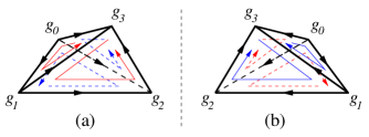
A generic SPT state with a finite symmetry group can be described by a path integral on a space-time lattice, or more precisely, a space-time complex with a branching structure. A branching structure can be viewed as an ordering of all vertices. It gives each link an orientation – which we can think of as an arrow that runs from the smaller vertex on that link to the larger one, as in Fig. 8. More generally, a branching structure determines an orientation of each -dimensional simplex, for every , including the top-dimensional ones that are glued together to make the full spacetime.
To each vertex , we attach a -valued variable . (Later we may also assign group elements to each edges .) An assignment of group elements to vertices or edges will be called a coloring. For a discrete version of the usual path integral of quantum mechanics, we will to sum over all the colorings. (See Sec. 9.1.) On a closed oriented space-time, in the Euclidean signature, the “integrand” of the path integral is given by
| (4.1) |
The argument of the path integral is a complex number with a nontrivial phase and thus it can produce complex Berry phases. We have written this formula for the case of dimensions, but it readily generalizes to any dimension. Here, for a given simplex with vertices depending on whether the orientation of that simplex that comes from the branching structure agrees or disagrees with the orientation of . The symbol represents a product over all -simplices.
Finally, and most importantly, the -valued is a homogeneous cocycle representing an element of . This means satisfy the cocycle condition , where
| (4.2) |
(The symbol is an instruction to omit from the sequence.)
We regard the complex phase as a quantum amplitude assigned to a -simplex in a -dimensional spacetime.
First, the path-integral model defined by the action amplitude eqn. (4.1) has a -symmetry
| (4.3) |
since the homogeneous cocycle satisfies
| (4.4) |
Second, because of the cocycle condition, one can show that
| (4.5) |
for any set of ’s, when the spacetime is an orientable closed manifold. This implies that the model is trivially soluble on a closed spacetime, and describes a state in which all local operators have short-range correlations. This state is symmetric and gapped. It realizes an SPT state with symmetry . The state is determined up to equivalence by the cohomology class of .
4.2 The first boundary of a generic SPT state – A simple model but with complicated boundary dynamics
So far, we have described a discrete system with symmetry on a closed -manifold . What happens if is an open manifold that has a boundary ? The simplest path-integral model that we can construct is simply to use all of the above formulas, but now on a manifold with boundary. Thus, the argument of the path integral is still given by eqn. (4.1), but now, this is no longer trivial:
| (4.6) |
Because of the properties of the cocycle, this amplitude only depends on the on the boundary, so it can be viewed as the integrand of the path integral of a boundary theory.
To calculate the path integral amplitude of the boundary theory, we can simplify the bulk so that it contains only one vertex (see Fig. 9). In this case, the effective boundary theory is described by a path integral based on the following amplitude:
| (4.7) |
This depends only on the boundary spins , and not on in the bulk. (This follows from the cocycle condition for . Readers who are not familiar with this statement can find the proof in Sec. 9.) Here, depending on whether the orientation of a given triangle that comes from the branching structure agrees with the orientation that comes from the triangle as part of the boundary of the oriented manifold . (Symbols like and similar notation below are shorthands for products over simplices, as written explicitly in the right hand side of eqn. (4.7).)
Since the path integral amplitude of the boundary theory is path dependent and not equal to 1, the dynamics of the simple model is hard to solve, and we do not know if the boundary is gapped, symmetry breaking, or topological. In fact, for cocycles that are in the same equivalence class but differ by coboundaries, the boundary amplitudes are different, which may lead to different boundary dynamics. In Sec. 3.1, for the case of the CZX model, we have chosen a particular cocycle in an equivalence class. This choice of cocycle leads to a gapless boundary.
4.3 Non-on-site (anomalous) -symmetry transformation on the boundary effective theory
4.3.1 Symmetry transformation on a spacetime boundary in Lagrangian formalism
We continue to assume that the spacetime manifold has a boundary , which can be regarded as a fixed-time slice on the closed space region . The effective theory eqn. (4.7) possesses the symmetry:
| (4.8) |
But this symmetry in the presence of a boundary is in fact anomalous (i.e. non-on-site). The anomalous nature of the symmetry along the boundary is the most important property of SPT states.
To understand such an anomalous (or non-on-site) symmetry, we note that locally (that is, for a particular simplex) the action amplitude is not invariant under the -symmetry transformation:
| (4.9) |
Only the total action amplitude on the whole boundary (here the boundary of an open manifold is a closed manifold) is invariant under the -symmetry transformation. (Readers who are not familiar with this statement can read the proof in Sec. 9.) Such a symmetry is an anomalous (or non-on-site) symmetry.
Since the action amplitude is not invariant locally, but invariant on the whole boundary , thus under the symmetry transformation, the Lagrangian may change by a total derivative term:
| (4.10) |
The presence of is another sign of the anomalous symmetry. To understand the symmetry transformation on the boundary in more detail, we note that, in our case, is given by
| (4.11) |
If we view
| (4.12) |
as a 2-cochain, it is actually a 2-coboundary (see Fig. 10):
| (4.13) | ||||
with a 1-cochain as
| (4.14) |

4.3.2 Symmetry transformation on a spatial boundary in Hamiltonian formalism
In the above, we have discussed the effective symmetry transformation on the spacetime boundary in Lagrangian formalism. Now we will proceed with a Hamiltonian formalism.
What we mean by a Hamiltonian formalism is to choose a fixed space , and use the path integral on to construct the imaginary-time evolution unitary operator , where represents the time direction (see Fig. 11). The matrix elements of the imaginary-time evolution operator is , where are the degrees of freedom on , and on . We may choose to represent just one time step of evolution, so that there are no interior degrees of freedom to sum over. In this case, the unitary operator are
| (4.17) |
When the space has a boundary, then some degrees of freedom live on the boundary and others live in the interior of . We can ask about the properties of global symmetry transformations in two scenarios: The first is the symmetry of the whole bulk and the boundary included together, which is an on-site symmetry. The second is the symmetry of the effective boundary theory only, which turns out to be a non-on-site symmetry.
-
1.
For the first scenario, the symmetry of the whole bulk and the boundary together, we have
because every homogeneous cochain satisfies . If we write the evolution operator explicitly, including the matrix elements and basis projectors, we see that
where generates the usual on-site -symmetry transformation . Thus, the -symmetry transformation on the whole system (with bulk and boundary included) is an on-site symmetry, as it reasonably should be as in condensed matter.
-
2.
For the second scenario, to obtain the symmetry of the effective boundary theory, we can simplify all the interior degrees of freedom into a single one , then the degrees of freedom on are given by where live on the boundary and lives in the interior of (see Fig. 11). Now the imaginary-time evolution operator is given by
(4.18) which defines an effective Hamiltonian for the boundary. Now, we are ready to ask: What is the symmetry of the effective boundary Hamiltonian, or effectively the symmetry of time evolution operator ?
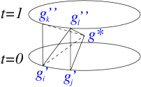
Figure 11: representing one step of imaginary time evolution, for the effective boundary theory. The space is given by the disk. The analysis of global symmetry in Sec. 4.3.1 no longer applies. The discrete time evolution operator does not have the usual global symmetry:
(4.19) since
(4.20) The difference between two matrix elements and is just a phase factor
(4.21) where multiplies over all the 3-simplices in Fig. 11, over all the 2-simplices on , over all the 1-simplices on the top and the bottom boundaries of . Note that many oppositely oriented terms are cancelled out in order to derive the last form of the above eqn. (2). This means that the boundary time evolution operator is invariant
under a modified -symmetry transformation
(4.22) where
(4.23) and generates the usual on-site -symmetry transformation . The phase factor makes the -symmetry to be non-on-site at the boundary.
We have written these formulas in 2+1 dimensions, but they all can be generalized. In dimensions, we have an effect boundary symmetry operator acting on for the effective boundary Hamiltonian :
(4.24)
4.4 The second boundary of a generic SPT state – Gapped boundary by extending the -symmetry to an -symmetry
In Sec. 3.1 and also in Sec. 4.2, we considered the path integral of a -SPT state described by a homogeneous cocycle . The path integral that we studied in that section remained -symmetry invariant even on a manifold with boundary, where the -symmetry is an on-site symmetry in the bulk. However, if we integrate out the bulk degrees of freedom, the effective boundary theory will have an effective -symmetry, which must be non-on-site (i.e. anomalous) on the boundary. This anomalous -symmetry on the boundary forces the boundary to have some non-trivial dynamical properties.
However, the simple model introduced in Sec. 4.2 has a complicated boundary dynamics, which is hard to solve. There are several standard ways to modify the construction in Sec. 4.2 to get a boundary that can be solved exactly. One way to do so is to constrain the group variables on boundary sites to all equal 1, or at least to take values in a subgroup such that the cohomology class of becomes trivial when restricted to . Given this, after possibly modifying by a coboundary, we can assume that when the group variables all belong to . In this case, the action amplitudes for the boundary effective theory eqn. (4.7) are always equal to 1 (after choosing ). So the boundary constructed in this way is exactly soluble, and is gapped. This construction amounts to spontaneous or explicit breaking of the symmetry from to .
In this section, we will explain another procedure to construct a model with the same bulk physics and an exactly soluble gapped boundary. This will be accomplished by extending (rather than breaking) the global symmetry along the boundary. Then, as in our explicit example of the CZX model in Sec. 3.2, we get a boundary state that is gapped and symmetric, but the symmetry along the boundary is enhanced relative to the bulk.
4.4.1 A purely mathematical setup on that -cocycle is trivialized in
To describe the symmetry extended boundary, let us introduce a purely mathematical result. We consider an extension of ,
| (4.25) |
where is a normal subgroup of , and . Here is a surjective group homomorphism from to . A “-variable” -cocycle can be “pulled back” to an “-variable” -cocycle , defined by
| (4.26) |
The case of interest to us is that is trivial in . This means can be rewritten as a coboundary, namely
| (4.27) |
(The symbol is an instruction to omit from the sequence.)
For the convenience and the preciseness of the notation, we can also shorten the above eqn. (4.27) to
| (4.28) |
where the variable in the bracket is a shorthand of many copies of group elements in a direct product group of . By pulling back a -cocycle back to , it becomes an -coboundary . Formally, we mean that a nontrivial -cocycle
| (4.29) |
becomes a trivial element when it is pulled back (denoted as ∗) to
| (4.30) |
Saying that this element is trivial means that the corresponding cocycle is a coboundary.
Here is a homogeneous -cochain:
| (4.31) |
The definition of also ensures that
| (4.32) |
since is trivial in for any . In particular, , and therefore
| (4.33) |
Thus when we restrict to , the cochain becomes a cocycle in . An important detail is that in general the cohomology class of is not uniquely determined by the original cocycle . In general, it can depend on the choice of cochain that was used to trivialize .
In fact, let and be two cochains, either of which could be used to trivialize :
| (4.34) |
Then is a cocycle, . So has a class in . If this class is nontrivial, the gapped boundary states that we will construct using and are inequivalent. Thus the number of inequivalent gapped boundary states that we can make by the construction described below (keeping fixed and ) is the order of the finite group .121212It is not true that these states can be classified canonically by , because there is no natural starting point, that is, there is no natural choice of to begin with. Once one makes such a choice, the boundary states that we will construct can be classified by .
A nontrivial class in may or may not remain nontrivial after restriction from to , so in general as stated above the cohomology class of can depend on the choice of .
4.4.2 -symmetry extended boundary — By extending -symmetry to -symmetry
To construct the second boundary of generic SPT state, we allow the degrees of freedom on the vertices at the boundary to be labeled by . This amounts to adding new degrees of freedom along the boundary. The degrees of freedom on the vertices in the bulk are still labeled by . With this enhancement of the boundary variables, we can write down the action amplitude for the second construction as
| (4.35) |
where and are the cochains introduced in the last section and may have a boundary. Here, if a vertex in is on the boundary, the corresponding is given by .
We note that, since : is a group homomorphism, the action : , , induces an action : , . Therefore, the total action amplitude eqn. (4.35) has symmetry:
| (4.36) |
where . In the bulk, the symmetry is , but along the boundary it is extended to . Such a total action amplitude defines our second construction of the boundary of a -SPT state, which has a symmetry extension lifted to on the boundary. We return to more details on this model in Sec. 9.
The bulk of the constructed model is described by the same group cocycle , which give rise to the -SPT state. But the boundary has an extended symmetry . In this case, we should view the whole system (bulk and boundary) as having an extended -symmetry, with the subgroup acting trivially in the bulk. So the effective symmetry in the bulk is .
The dynamics of our second boundary is very simple, since the total action amplitude eqn. (4.35) is always equal to 1 by construction:
| (4.37) |
where . Thus, the ground state is always gapped and there is no ground state degeneracy regardless of whether the system has a boundary or not. In other words, the second boundary of the -SPT state is gapped with symmetry and no topological order. The gapped boundary with symmetry and no topological order is possible, since we have chosen so that when we view the -SPT state as an -SPT state, the non-trivial -SPT state becomes a trivial -SPT state.
4.5 On-site (anomaly-free) -symmetry transformation on the boundary effective theory
Now we show that symmetry extension, as described in Sec. 4.4.2, gives a boundary state with on-site (anomaly-free) -symmetry, based on the Hamiltonian formalism on the boundary. This section directly parallels the previous discussion in Sec. 4.3, where a non-trivial -cocycle gives rise to a non-on-site effective -symmetry on the boundary. After extending the symmetry to , the non-trivial -cocycle becomes a trivial -cocycle , which in turn gives rise to an on-site effective -symmetry for the boundary effective theory.
Taking as an example, Eqns. (4.13), (4.14) and (4.15) of Sec. 4.3.1 still hold. Furthermore, when , and are boundary degrees of freedom in , eqn.(4.13) becomes
| (4.38) |
See Fig. 12 for an illustration. Here is a homogeneous 2-cochain that splits (or ) and satisfies . Now the split 2-cochain in eqn.(4.14) has a new form:
| (4.39) |
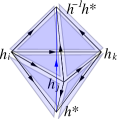
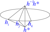
To show more clearly that -symmetry can be made on-site and anomaly-free in any dimension , we note that the action amplitude eqn. (4.35) can be rewritten as
| (4.40) |
Each local term is already invariant under -symmetry transformation on the boundary. So we will drop it. The term may not be invariant under -symmetry transformation on the boundary, although their product is. This may lead to a non-on-site -symmetry. Repeating the calculation in Sec. 4.3, we found that the discrete time evolution operator does not have the usual global symmetry, where their matrix elements follow:
| (4.41) |
But it is invariant
under a modified symmetry transformation operator
| (4.42) |
which appears to be non-on-site. However, since is a coboundary, the above can be rewritten as (see Fig. 11 and 13)
| (4.43) |
After a local unitary transformation with
we can change the above -symmetry transformation to
| (4.44) |
which indeed becomes on-site. The on-site symmetry makes the time evolution operator invariant under
4.6 The third boundary of a generic SPT state: A gapped symmetric boundary that violates locality with (hard) gauge fields
In the last section, we constructed a gapped symmetric boundary of an SPT state such that the global symmetry is extended from to along the boundary. Such boundary enhancement of the symmetry is usually131313In Sec. 3.2, we described a situation in which it is natural. not natural in condensed matter physics. Just as in our discussion of the CZX model in Sec. 3.3, 3.4, the way to avoid symmetry extension is to gauge the boundary symmetry , giving a construction in which the full global symmetry group is (or in the more general mixed breaking and extension construction described in Sec. 8.2).
As in the CZX model, there are broadly two approaches to gauging the symmetry. One may use “hard gauging” in which one introduces (on the boundary) elementary fields that gauge the symmetry, or “soft gauging” in which the boundary gauge fields are emergent. Hard gauging is generally a little quicker to describe, so we begin with it, but soft gauging, which will be the topic of Sec. 4.7, is more natural in condensed matter physics because it can be strictly local or “on-site.” Our discussion here and in the next section is roughly parallel to Sec. 3.3 and 3.4 on the CZX model.
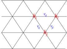
To construct a new boundary, let us consider a system on a -dimensional space-time manifold , with a triangulation that has a branching structure. A vertex inside carries a degree of freedom . A vertex on the boundary carries a degree of freedom . A link on the boundary carries a degree of freedom . See Fig. 14
We choose the action amplitude of our new model to be
| (4.45) | ||||
where is a product over -dimensional simplices in the bulk, and is a product over -dimensional simplices on the boundary. is the orientation of the -simplex , and is the orientation of the -simplex . Finally, will be defined in Sec. 4.6.1, using introduced in Sec. 4.4.1, as well as “hard gauge fields” along boundary links.
In the action amplitude eqn. (4.45), is the cocycle describing the -SPT state. We have assumed that if a vertex in is on the boundary, then the corresponding is given by .
4.6.1 A cochain that encodes “hard gauge fields”
The generalized cochain will be defined for boundary simplices. It will depend on -valued boundary spins as well as -valued boundary link variables . As usual in lattice gauge theory, we can regard as a gauge connection on the link .
First, we assume that for any configurations that do not satisfy , for some , , . So only the configurations that satisfy
| (4.46) |
on every triangle can contribute to the path integral. This means that only flat gauge fields are allowed.
For a flat connection on a simplex with vertices , all of the can be expressed in terms of . So likewise can be expressed as . We define in terms of the homogeneous cochain of Sec. 4.4.1 by
| (4.47) |
In other words
| (4.48) |
where is given by parallel transported from site- to site- using the connection :
| (4.49) |
We note that has a local -symmetry generated by :
| (4.50) |
Next we will view such a boundary local symmetry as a -gauge redundancy by viewing two boundary configurations and as the same configuration if they are related by a gauge transformation
| (4.51) |
Eqn. 4.6.1 ensures the gauge-invariance of the boundary action.
Now that we have gauged the symmetry, the global symmetry of the full system, including its boundary, is . However, viewing two boundary configurations and as the same configuration makes the gauged theory no longer a local bosonic system. This is because the number of different (i.e. gauge inequivalent) configurations on the space-time boundary is given by141414The formula works when all groups are Abelian. For non-Abelian groups, there could be additional constraints on this formula, for example, in terms of conjugacy classes.
| (4.52) |
where is the number of vertices, is the number of links on the boundary , and is the number of elements in the Set. Here we count all the distinct configurations of vertex variables of and link variables of , identifying them up to -gauge transformations on the vertices. We consider all higher energetic configurations, which include both flat and locally non-flat configurations, much more than just ground state sectors. Constant gauge transformations yield an additional factor . The appearance of the factor whose exponent is not linear in and implies a non-local system. So the third boundary is no longer local in that strict sense. In subsection 4.6.2, we show that this non-local boundary is gapped and symmetric. In Sec. 4.7, we will replace hard gauging with soft gauging and thereby get a boundary that is fully local and on-site, while still gapped and symmetric.
4.6.2 A model that violates the locality for the boundary theory
In the path integral, we only sum over gauge distinct configurations:
| (4.53) | ||||
where represents the gauge equivalence classes. (Equivalently, we can sum over all configurations and divide by the number of equivalent configurations in each gauge equivalence class.)
We emphasize:
“Since the boundary theory is non-local respect to the boundary sites, it is no longer meaningful to distinguish on-site from non-on-site symmetry, or anomaly-free from anomalous symmetry.”
However, this system does have a global symmetry. To see this, let us consider a transformation generated by given by
| (4.54) |
if is on the boundary, and
| (4.55) |
if is in the bulk. Clearly, such a transformation is actually a transformation in the bulk. On the boundary, since and are gauge equivalent for , and generate the same transformation. So the transformation on the boundary is given by the equivalence class under the equivalence relation , . Since is a normal subgroup of , the equivalence classes form a group . Thus, the transformation is also a transformation on the boundary. Such a transformation is a symmetry of the model since
| (4.56) |
where we have used the definition eqn. (4.6.1). We note that since is a normal subgroup of . So the partition function eqn. (4.53) gives us a boundary effective theory that still has the global symmetry.
Now we can ask whether the ground state at the boundary breaks the -symmetry or not. More generally, what is the dynamical property of such a boundary? Is it gapped? To answer such a question, we note that on a triangulated , in general
| (4.57) |
since has a boundary. But we can show that if the boundary is simply-connected, then
| (4.58) | |||
To show this, we first recall that only flat connections on the boundary contribute to the path integral. If the boundary is simply-connected, this means that we can assume that is pure gauge. So by a gauge transformation eqn. (4.6.1), we can set all to on the boundary:
| (4.59) |
where is obtained from by the gauge transformation that sets the to 1. But this is 1 by virtue of eqn. (4.4.2).
The fact that the action amplitude of our theory on is always one if the boundary of is simply-connected is enough to show that the system on is in a gapped phase both in the bulk and on the boundary. Such a gap state is the -gauge deconfined state, described by the flat -connection on each link. Also and are strongly fluctuating and are quantum-disordered as well. This is because the action amplitude is always equal to 1 regardless the values of and (say, in the gauge discussed above). So the partition function eqn. (4.53) gives us a boundary of the SPT state that is in the deconfined phase of -gauge theory, and does not break the symmetry.
4.7 The fourth boundary of a generic SPT state: A gapped symmetric boundary that preserves locality with emergent (soft) gauge fields
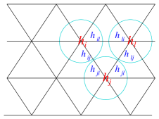
In the last section, we constructed a gapped symmetric boundary of an SPT state by making its boundary non-local. In this section, we are going to fix this problem, by constructing the fourth gapped symmetric boundary of an SPT state without changing the symmetry and without destroying the locality. The new gapped symmetric boundary has emergent gauge fields and topological order on the boundary. By this explicit construction, we show that:
“In 3+1D and any higher dimensions, an SPT state with a finite group symmetry, regardless unitary or anti-unitary symmetry, always151515To complete the argument, we need to know that for every SPT phase with symmetry, a suitable extension exists. This is shown in Sec. 5. has a gapped local boundary with the same symmetry.”
The construction in this section is a generalization of the construction in Sec. 3.4.
To construct a local boundary, we replace on a link by two degrees of freedom and . In other words, a link on the boundary now carries two degrees of freedom and (see Fig. 15). We regard as the degrees of freedom on site- of the boundary (see Fig. 15). In the bulk, a site- only carries a degree of freedom described by .
We choose the action amplitude for our fourth boundary to be
| (4.60) | ||||
In the following, we will define . We introduce a new form of cochain encoding “soft gauge fields” emergent from the local boundary sites that we prescribe below.
4.7.1 A new cochain that encodes “emergent soft gauge fields”
First, we assume that for any configurations that do not satisfy
| (4.61) |
for every link or do not satisfy
| (4.62) |
for every triangle. So only the configurations that satisfy
| (4.63) |
on every triangle contribute to the path integral. Here corresponds to the -gauge connection introduced in the last section.
The -gauge symmetry will impose the equivalence relation
| (4.64) |
for any . The total number of inequivalent configurations on space-time boundary is given by
| (4.65) |
The exponent in the number of configurations is linear in and , implying that the system is local.
Let us further assume that depends on only via . So we can express as . We can simplify this further: The non-zero can be expressed via . In other words, on all the links of a -simplex can be determined from a subset .
At this stage, we simply define via eqn. (4.6.1), but using the effective gauge fields defined in eqn. (4.63) to replace the hard gauge fields that were assumed previously. The resulting model is manifestly gauge invariant, just as it was before. However, hard gauging has now been replaced with soft gauging, making the model completely local, both in the bulk and on the boundary. In this case, the global symmetry is on-site for the whole system (including bulk and boundary). But if we integrate out the gapped bulk, and consider only the effective boundary theory, we would like to ask if the effective global symmetry on the boundary is on-site or not? Since this point is important, we elaborate on it in the next section.
4.7.2 The locality and effective non-on-site symmetry for the boundary theory
We have shown that the model obtained by soft gauging is local both in the bulk and on the boundary. If we integrate out the bulk degrees of freedom, we get an effective boundary theory, whose action amplitude is given by a product of terms defined for each boundary simplex. The total boundary action amplitude is invariant under the -symmetry transformation on the boundary, but each local term on a single boundary simplex may not be. This leads to a possibility that the effective boundary -symmetry is not on-site. We have constructed two boundaries that are local in Sec. 4.2 and 4.4. The first boundary in Sec. 4.2 has a non-on-site effective -symmetry on the boundary, while the second boundary in Sec. 4.4 has an on-site effective -symmetry on the boundary.
In the path integral, we only sum over gauge distinct configurations:
| (4.66) | ||||
where represents the gauge equivalence classes.
Such a lattice gauge theory with soft gauging will have an on-site global symmetry . To see this, let us consider a transformation generated by on site . It is given by, if is on the boundary,
| (4.67) |
and, if is in the bulk,
| (4.68) |
Such a transformation is a transformation in the bulk. On the boundary, since and are gauge equivalent for , and generate the same transformation. So the transformation on the boundary is given by the equivalence class under the equivalence relation , . Since is the normal subgroup of , the equivalence classes form a group . Thus, the transformation is also a transformation on the boundary. Such a transformation is on-site, and is a symmetry of the model since each term in the action amplitude, such as and , is invariant under the -symmetry transformation: and
| [used the definition eqn. (4.61)] | |||||
| [used the definition eqn. (4.6.1)] | |||||
| (4.69) | |||||
To see if the effective boundary -symmetry is on-site or not, we first note that the term in the total action amplitude, , is purely a boundary term. Each contribution from a single boundary simplex is already invariant under the -symmetry transformation (see eqn. (4.7.2)). So, such a term will not affect the on-site-ness of the effective boundary symmetry, and we can ignore it in our discussion.
The other term may lead to non-on-site effective boundary symmetry. But the calculation is identical to that in Sec. 4.3. We find that the resulting effective boundary -symmetry is indeed non-on-site if the -cocycle is not a coboundary.
So the partition function eqn. (4.66) gives us a boundary effective theory that still has the symmetry, as well as a local Hilbert space. (The boundary does not break or extend the -symmetry.) But the effective symmetry on the boundary is non-on-site (i.e. anomalous).
The dynamical properties of the soft gauging model in Sec. 4.7 are the same as in the hard gauging case in Sec. 4.6, since the two path integrals are manifestly the same. In particular, this is a physically satisfactory construction of a symmetry-preserving gapped boundary of a bulk SPT phase with global symmetry . The boundary is topologically ordered with emergent -gauge symmetry. The -gauge theory is in a deconfined phase, which we discuss further in Sec. 4.8. The boundaries of the CZX model discussed in Sec. 3.4 and Appendix A.2 are examples of this general construction.
4.8 Gapped boundary gauge theories: -symmetry preserving (2+1D boundary or above) or -spontaneous symmetry breaking (1+1D boundary)
To identify the boundary -gauge theory, we look more closely at the boundary factors in the path integral (4.45). To understand the boundary theory in isolation, it is convenient to consider the case that all are equal to 1, which ensures that the boundary spins are -valued. The boundary theory is now just a theory of -valued variables with an action amplitude that is given by the product over all boundary simplices of the generalized cochain that was defined in eqn. (4.6.1).
If we choose the spacetime to be a -ball , then the action amplitude in eqn. (4.66) is always equal to one regardless the values of in the bulk and ’s on the boundary (that satisfy eqn. (4.63)). Thus the system on a spacetime is in a gapped phase both in the bulk and on the boundary. Such a gapped state is the -gauge deconfined state, since the -connections are always flat thus .
Does such a -gauge deconfined state spontaneously break the -symmetry? We note that, except the combinations that are not fluctuating, other combinations of ’s are strongly fluctuating and quantumly disordered. Also and are strongly fluctuating and quantumly disordered. In fact, the model described by eqn. (4.66) has a local symmetry161616Here the local symmetry does not mean the gauge symmetry. On one hand, the local symmetry is that physically distinct configurations [note that in the main text discussion, two distinct configurations are and ] have the same action amplitude. On the other hand, the gauge symmetry is not a (global) symmetry but indeed a gauge redundancy. The gauge symmetry is a gauge redundancy that two (redundant) configurations are indeed the same equivalent physical configuration, and are related to each other through gauge transformations.: The action amplitude for configuration is the same as the action amplitude for configuration where generate the local -symmetry on gauge-invariant states. This is because the action amplitude is always equal to 1 regardless of the values of , and on a spacetime (as long as is satisfied). This local -symmetry allows us to show that any -symmetry breaking order parameter that can be expressed as a local function of will have a short-range correlation.
However, such a result is not enough for us to show all -symmetry breaking order parameters that are local operators to have short-range correlations. This is because some local operators are not local functions of , such as the operator that corresponds to a breakdown of the flat-connection condition . On a 1+1D boundary, such kinds of local operators can change the holonomy of the -gauge field around the space of the boundary. As discussed in Sec. 3.4, it is the order parameter that changes the holonomy that acquires a long-range correlation.
Therefore, we need to find a more rigorous way to test the spontaneous breaking of the -symmetry. One way to do so is to calculate the partition function eqn. (4.53) on a spacetime , which is given by the number of configurations that satisfy that the flat-connection condition and the condition . When is Abelian, we find the partition function to be171717 Here let us focus on the case that is Abelian (while and may be non-Abelian), for the simplicity of the formulas. One may generalize the situation to non-Abelian groups as well.
| (4.70) |
Let us explain the above result. The ’s on the vertices in the bulk contribute the factor to the total configurations, where is the number of vertices in the bulk (not including the boundary). The ’s on the vertices on the boundary contribute the factor to the total configurations, where is the number of vertices on the boundary. The of the link on the boundary can be labeled by , where and . The ’s contribute the factor , where is the number of links on the boundary. The needs to satisfy flat-connection condition , and the counting is complicated. When is Abelian, ’s contributes to a factor which comes from of the form , . But those are only contributions from the “pure gauge” configurations. There is another factor which is the number of inequivalent -gauge flat connections on . Last, we need to divide out a factor due to the -gauge redundancy eqn. (4.64).
The volume-independent partition function is given by
| (4.71) |
which is a topological invariant on spacetime with a vanishing Euler number [54]. If we choose , then will be equal to the ground state degeneracy on space:
| (4.72) |
Our strategy here is to test the ground state degeneracy caused by spontaneous symmetry breaking, based on the degeneracy of a spatial sphere on the boundary of a spatial bulk . Namely, we compute . Our argument relies on
“No ground state degeneracy on a spatial boundary sphere means no spontaneous symmetry breaking.”
Here we show that on a 1+1D spatial boundary of a 2+1D bulk, the GSD is , and we cannot exclude the possibility of spontaneous -symmetry breaking. On a 2+1D spatial boundary of a 3+1D bulk, or any higher dimensions, the GSD is , and there is no spontaneous -symmetry breaking.
We note our result here on the spontaneous symmetry breaking of 1+1D deconfined -gauge theory is consistent with other independent checks from a Hamiltonian approach of Sec. 3.3 and Appendix A.2.4, and a field theory approach of Appendix D.22.
As explained in Sec. 4.4.1, once all the variables are -valued, reduces to a cocycle appropriate for a gauge theory. As a result, the boundary factor in the path integral in eqn. (4.53) or eqn. (4.66), when the are 1, is just the action amplitude of a -gauge theory deformed with the cocycle , as in Dijkgraaf-Witten theory. This is the boundary state that has been coupled to the bulk -SPT phase to give a gapped symmetric boundary.
In general, not all variants of gauge theory can occur in this way, because there may be some that do not come from any . Restriction from to gives a map . The versions of -gauge theory that arise in our construction are the ones associated to classes that are in the image of . In general, if a given version of -gauge theory can arise by our construction as the gapped boundary of a given -SPT state, it can arise in more than one way. The number of ways that this can happen is the kernel of , which equals the number of classes in that map to a given class in .
5 Find a group extension of that trivializes a -cocycle

5.1 Proof: Existence of a finite -extension trivializing any finite ’s -cocycle in for
The construction in the last section gives a symmetric gapped boundary for the -SPT state associated to a -cocycle , provided that we can find an extension of ,
| (5.1) |
such that the -cocycle becomes trivial when pulled back to an -cocycle by . In this section, we will give an explicit construction of such an extension for any finite group , and for any -cocycle when . This approach works for -cocycles with , thus the bulk dimension of -SPT state has to be greater than or equal to D. Based on this method, below we show that a suitable group extension always exists, thus we prove that within group cohomology construction,
Statement 1: “Any bosonic SPT state with a finite onsite symmetry group , including both unitary and anti-unitary symmetry, can have an -symmetry-extended (or -symmetry-preserving) gapped boundary via a nontrivial group extension by a finite , given the bulk spacetime dimension .”
To motivate the construction, we start with the non-on-site symmetry discussed in Sec. 4. We can make the non-on-site symmetry to be on-site by splitting on each vertex on the boundary into several variables , , , etc., one for each attached simplex (see Fig. 16). In the Euclidean signature, we take the new evolution operator
| (5.2) |
to be non-zero only when on each vertex. In other words, if the condition is not satisfied on some vertices, then the configuration will correspond to high energy boundary excitations on those vertices.
In the new boundary Hilbert space spanned by , the symmetry transformation
| (5.3) |
becomes on-site (or on-cell, or on-simplex). On each simplex, the symmetry transformation is given by
| (5.4) | |||
Thus we can make any non-on-site symmetry on the boundary into an on-site symmetry, by redefining the boundary sites. This seems to contradict our picture that the non-on-site symmetry on the boundary captures the bulk SPT state, which should not be convertible into on-site boundary symmetry by any boundary operations (that have the local site structure).
In fact, there is no contradiction since may not generate the group . They may generate a bigger group – an extension of by an Abelian group . So after we split into , , etc. on the boundary, the symmetry of our model is no longer . It is changed into . Since the symmetry transformation generated by is on-site, such a symmetry transformation is not anomalous. The bulk -SPT state can also be viewed as an -SPT state. But as an -SPT state, it is the trivial one, since the the -symmetry is on-site on the boundary.
So, we have found an extension of , under , where is an Abelian normal subgroup of , such that
| (5.5) |
defined as
| (5.6) |
is trivial in . We also note that is a local symmetry (on each simplex) of the effective boundary Hamiltonian.

To calculate from , we consider three symmetry transformations , , and . We find that (see Fig. 17)
| (5.7) |
The above phase factor , as a function of , is a generator of the group . We can obtain all the generators by choosing different and , and in turn obtain the full group . We note that, due to the geometry nature of Fig. 17 and its generalization in dimensions , the above construction is true only for .
Thus, this concludes our proof of Statement 1. We can rephrase it to the equivalent proved statements:
Statement 2: “Any -cocycle of a finite group (a bosonic SPT state with a finite onsite, unitary or anti-unitary symmetry, symmetry group ), can be pulled back to a finite group via a certain group extension by a finite , such that . Namely, a -cocycle becomes a -coboundary, split to -cochains , given the dimension (q.e.d).”
Statement 3: “Any -anomaly in D given by of a finite group , can be pulled back to a finite group via a certain group extension by a finite , such that -anomaly becomes -anomaly free, given the dimension (q.e.d).”
Unfortunately, we do not have a systematic understanding of what will be generated by this construction. In particular, may be different for cocycles that differ only by coboundaries. Another drawback of this method is that we cannot obtain the exact analytic function of the split -cochain easily.
However, we provide a different method that helps to derive the analytic -cochain, based on the Lydon-Hochschild-Serre spectral sequence in Appendix D.3. Readers can find more systematic examples in Appendix D. Finally, we remark that very recently Ref. [55] has proven statements related to ours in a more mathematical setup.181818After the appearance of our preprint on arXiv, one of the authors (J.W.) thanks Yuji Tachikawa for informing the recent Ref. [55]’s Sec. 2.7 of as a mathematical proof, reproducing and obtaining similar results as our Sec. 5.1.
5.2 2+1/1+1D and /D Bosonic SPTs for an even : The D -gauge theory boundary of D bulk invariant via
We would like to apply the above method to some cocycles that describes SPT states. For example, we can consider a non trivial cocycle in .
| (5.8) |
where . Choose , and , we find
| (5.9) |
In fact, , and
| (5.10) |
So and . The short exact sequence trivializes the cocycle .
See Appendix D.4 for further illumination of this example. In general, we find that in any odd spacetime dimension, there is a -SPT phase and that a gapped symmetric boundary for this phase can be obtained from the extension . See Appendix D.5. The bulk SPT phase is associated to the invariant with a cup product form of , a nontrivial element in for an even . The here is a -valued 1-cocycle in on the spacetime complex .
5.3 3+1/2+1D and /D Bosonic topological superconductor with time-reversal symmetry for an odd : The D -gauge theory boundary of D bulk invariant via
Next, we consider a non trivial cocycle [15]. The represents a nontrivial class of bosonic SPTs with an anti-unitary time-reversal symmetry. This SPTs is also named as bosonic topological superconductor or bosonic topological paramagnet with . Here and are the same group mathematically. However, the generator in provides a non-trivial action on the -module , denoted as . The subscript in the module indicates that the group has a non-trivial action on the module.
More generally when a group contains an anti-unitary operation such as time-reversal , we define a nontrivial -module as . We stress that and are the same Abelian group. The group action is only non-trivial when , for , , such that if contains an anti-unitary element, and if contains no anti-unitary element. The formalism developed in this paper up to this point is applicable to this case, for models that fit in the group cohomology framework.
The group cocycle of this SPT phase is given by
| (5.11) |
where . Choose , and , we find
| (5.12) |
and . In fact, we obtain
| (5.13) |
So and . The short exact sequence trivializes the cocycle . This means that becomes a coboundary in for a larger group . Thus, we find that the 3+1D bosonic SPTs with symmetry (the bosonic topological superconductor of ) has a 2+1D symmetry-preserving surface topological order.
For the boundary -gauge theory of a -SPT state, the gauge charge excitations are labeled by Rep=Rep() with , instead of Rep=Rep. is a “twisted” product of and , the so-called projective symmetry group (PSG) introduced in Ref. [46]. When a gauge charged excitation is described by Rep instead of Rep, it implies that the particle carries a fractional quantum number of global symmetry . We say there is a fractionalization of the symmetry .
We note that the surface topological order first proposed in [30] on the surface of 3+1D -bosonic topological superconductor is also a 2+1D deconfined gauge theory.
See Appendix D.6 for further illumination of this example. In general, we find that the construction can provide a boundary D gauge theory on D bosonic -SPTs, when is odd, see Appendix D.7. The bulk SPT invariant is equivalent to the partition function for an odd , a nontrivial element in . The here is a -valued, the first Stiefel-Whitney (SW) class in on the spacetime complex . Here is the of a spacetime tangent bundle over . The holds on a non-orientable manifold.
More examples of symmetry-extended gapped boundaries are provided in Appendix D.
6 Boundaries of SPT states with finite/continuous symmetry groups and beyond group cohomology
In the above Sec. 5, we described a method that constructs exactly soluble boundary for any within-group-cohomology SPT states with a finite symmetry group , via a nontrivial group extension by a finite group . Those boundaries preserve the -symmetry and have topological orders if the boundary dimension is 2+1D and higher. Such a result can be generalized to SPT states with a continuous compact symmetry group , provided that the group cocycle that describes the -SPT state can be trivialized by a finite extension , namely, with a finite group . This is because even for a continuous compact symmetry group , the action amplitude in eqn. (4.53) is still always equal to one regardless of the values of in the bulk and ’s on the boundary. Thus eqn. (4.70) is still valid if we treat and as the volumes of the continuous group and . When is finite, the flat condition makes the -gauge theory in a gapped deconfined phase. Therefore, for both a finite group and a continuous compact group , a D -SPT state within group cohomology can have a symmetry preserving gapped boundary if the -group cocycle can be trivialized by a finite extension of and when .
The SPT states within group cohomology have pure gauge -anomalies on the boundary corresponding to the global symmetry group . More general SPT states exist that have mixed gauge-gravitational anomalies on the boundary [17]. Those SPT states are referred to as beyond-group-cohomology SPT states [30]. Those beyond-group-cohomology SPT states can be constructed using group cohomology of . More precisely, using the action amplitude constructed from the group cocycle , we can construct models that realize the beyond-group-cohomology SPT states (as well as within group-cohomology SPT states) in D [17]. However, the correspondence between -cocycle and a D -SPT state is not one-to-one: Several different cocycles can correspond to the same SPT state.
We note that [17]
| (6.1) |
The cocycles in the first term describe invertible topological orders which do not need the symmetry group . The cocycles in the second term will describe -SPT states in a many-to-one fashion.
When is finite, a cocycle in can always be trivialized by an Abelian extension : . This is because when , then the can be viewed as a part of , and we can use the approach in Sec. 5 to show that the cocycles in can always be trivialized by a finite extension of . When , we note that . Using the approach in Sec. 5, we can show that the cocycles in can always be trivialized, which in turn allows us to show that the cocycles in can always be trivialized.
This allows us to conclude that the bosonic D beyond-group-cohomology -SPT states described by always have a symmetry preserving gapped boundary when is finite and when the bulk space dimension . Here can contain anti-unitary symmetries including time-reversal symmetry.
7 Boundaries of bosonic/fermionic SPT states: Cobordism approach
In principle, the philosophy of our approach should also work for the cobordism group description of topological states. For example, based on Ref.[18], one can consider bosonic SPTs in a -dimensional spacetime with a finite internal onsite symmetry group via a cobordism theory. Such an SPT state is proposed to be classified by
| (7.1) |
which is called the Pontryagin-dual of the torsion subgroup of the oriented bordism group . In the first equality of eqn. (7.1), the is called the oriented cobordism group of with coefficient, it is defined as , the space (here an Abelian group) of homomorphisms from to . The is a map defined as . The image of the map is composed by elements of that vanish on the torsion subgroup of bordism group, . Effectively, this yields the second equality, the is equivalent to , namely the space (here again an Abelian group) of homomorphisms from the torsion subgroup of bordism group to .
To determine the symmetry-extended gapped interface of a -SPT state, we need to find a larger total group that forms a group extension by a finite group . By pulling back to , we require that the nontrivial element in specifying a -SPT state, becomes a trivial identity element in the Cobordism group , where Hom . In short, the -SPT state within Cobordism group becomes a trivial -SPT state (a trivial vacuum in ) within Cobordism group . The boundary of such a -SPT state should allow a -symmetry-preserving gapped interfaces with a deconfined topologically ordered -gauge theory (where is a finite discrete group), if the spacetime dimensions of bulk dimension , above or equal to D.
The above procedure is for bosonic SPT states including only fundamental bosons. For fermionic SPT states including fundamental fermions, in principle, we can replace the oriented in Cobordism groups and , to the Spin version of Cobordism groups for the fermionic SPT states (namely and ), and to the Pin± version of Cobordism groups for the fermionic SPT states with time reversal symmetries (namely and ), where for or for , respectively [20]. The is the fermion-number parity. In this setup, our approach for symmetric gapped interfaces should be applicable to both bosonic and fermionic SPT states. The underlying idea again is related to the fact that a certain global anomaly associated to on the boundary of -SPT states becomes anomaly-free in a larger group .
It will be interesting to find more concrete examples and figure out the explicit analytic (exactly soluble or not) lattice Hamiltonian construction for such symmetry-preserving gapped boundaries within the cobordism setup in the future.
8 Generic gapped boundaries/interfaces: Mixed symmetry breaking, symmetry extension and dynamically gauging
In this section, we will give an overview of how the symmetry extension construction we have described is related to what may be more familiar gapped boundary states. We will also describe the generalizations of the ideas to interfaces between SPT states, and to the case that the bulk phase has intrinsic topological order. We will further develop their path integrals, lattice Hamiltonians and wave functions suitable for many-body quantum systems in Sec. 9.
8.1 Relation to Symmetry Breaking
The most familiar type of gapped boundary state for a -SPT phase is obtained by explicitly or spontaneously breaking the symmetry on the boundary to a subgroup of . Here must have the property that the cocycle defining the -SPT phase becomes a coboundary when the variables are restricted from to . For the notational distinction, we call this unbroken subgroup of as .
From the point of view of this paper, the statement that is a subgroup of means that there is an injective homomorphism . A gapped boundary state can be constructed if the given cohomology class in is trivial when pulled back to . See Appendix F.1 for explicit examples.
8.2 Symmetry Extension and Mixed Symmetry Breaking/Extension
Our construction on the symmetry extension in this paper is instead based on a surjective, rather than injective, homomorphism . Because is surjective, the symmetry is extended (from to ) along the boundary, rather than being broken. By gauging , one can arrange so that the global symmetry of the full system is . Many examples of symmetry-extended gapped boundaries are shown in Appendix D.
It is straightforward to combine the two cases. We can construct a gapped boundary state associated to any homomorphism , such that the cohomology class in becomes trivial when pulled back to . The construction proceeds exactly as we have explained in earlier sections of this paper, without any substantial modification. In this boundary state, is spontaneously or explicitly broken to the subgroup , and then is extended to .
More explicitly, one could also imagine arranging the above procedure in a two-stage process. Assume that in a layer within a distance from the boundary, is spontaneously broken down to . Then near the boundary the global/gauge symmetry is only and the boundary condition is defined by the choice of a group , with a surjective map to , such that the cocycle of becomes trivial by lifting to : via . In other words, to construct a boundary condition in a mixed symmetry breaking/extension case, what we need is that the cocycle of that defines the bulk topological state, when restricted to and then pulled back to , becomes trivial.
In all of these cases, one has to actually pick a trivialization of the pullback of to . The possible choices differed by a class in correspond to an -topological state on the boundary. This corresponds roughly to appending an -topological state on the boundary.
8.3 Gapped Interfaces
One can similarly consider the case of an interface (i.e. domain wall) between two SPT phases. In general, we may have one symmetry group on one side of the interface, with a cohomology class , and a second symmetry group on the other side, with its own cohomology class . (The gapped boundary of -topological state can be regarded as a gapped interface between a -topological state and a trivial vacuum.) We shall describe gapped interfaces between these two states.
Interfaces can be reduced to boundary states by a well-known folding trick. Instead of saying that there is on one side and on the other side, one “folds” along the interface and considers a system with a combined symmetry group , and a cohomology class . (Folding inverts one of the two cohomology classes.) Then we can construct gapped interfaces associated as above to any homomorphism .
An interesting special case is that the same group is supposed to be unbroken on both sides and also along the interface. This means that , and that the unbroken subgroup is a diagonal subgroup of . The cohomology class of restricts to a class of that we can denote by the same name. can be any finite extension of that trivializes this class.
8.4 Intrinsic Topological Order
Though our emphasis in this paper has been on gapped boundary states for SPT phases, a similar construction applies to bulk phases with intrinsic topological order.
We can construct such a phase simply by gauging the symmetry of a given -SPT state. Then since is extended to along the boundary, for consistency we have to gauge the full symmetry along the boundary. All our formulas make sense in that context.
SET phases can be treated in a similar way. For this, we gauge a subgroup of . The most significant case is that is a normal subgroup of . Then gauging gives a state with intrinsic topological order of an -gauge theory, in which is a quotient group of global symmetries. Along the boundary, we have to gauge the inverse image of in . If the map is surjective, then the symmetry remains as a symmetry of the boundary state and is extended along the boundary to the inverse image of in . For details see again Sec. 9. It is again possible to consider more general cases in which the symmetry may be partly broken along the boundary and partly extended.
There is no essential loss of generality in assuming here that is a normal subgroup of , for the following reason. If is not normal, then gauging will explicitly break to a subgroup , the normalizer of in . Then is normal in . After replacing by , everything proceeds as before.
9 General construction of exactly soluble lattice path integral and Hamiltonian of gapped boundaries/interfaces for topological phases in any dimension
We consider the spacetime-lattice path integral formulation in Sec. 9.1 and the spatial lattice Hamiltonian formulation in Sec. 9.2 for a systematic construction of gapped boundaries/interfaces for topological phases in any dimension. See Table 9 for an example of the lattice formed by simplices on a space or spacetime complex.
9.1 Path integral
In the following subsections, we systematically construct the path integral defined for various topological phases (including SPT, gauge theory, SET, gapped boundary/interfaces, etc) and contrast their properties. We shall clarify the gauge equivalent configuration briefly mentioned in eqn. (4.53), and the precise mod-out factor to remove the symmetry/gauge redundancy. In Sec. 4.7, we showed the construction of cocycle that contains the emergent gauge fields. We call this type of gauge field is soft gauged, which means that the Hilbert space of the gauge theory is still a tensor product form defined on each local site. , because the are variables assigned to the site (see Fig. 15). Below we discuss the hard gauged theory, where the total Hilbert space is not a tensor product form of Hilbert spaces on each local site since we require additional link variables.
We should note that we can easily formulate a soft gauge theory from a hard gauge theory, based on Sec. 4.7. One reason to consider the hard gauge theory in the following Secs. 9.1.2 and 9.1.3 is for the simplicity of notation and calculation, and for its smaller Hilbert space.
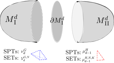
(1)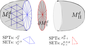 (2)
(2)
Schematically Figs.18 and Fig.19 summarize how to define an exactly soluble partition function or path integral on a triangulated spacetime complex. Normally, a path integral of gapped topological phase is well-defined on a closed spacetime manifold. However, here in particular, some path integral of fully gapped topological phase is also well-defined in the gapped bulk on with a gapped interface .
9.1.1 SPTs on a closed manifold
We start from reviewing and strengthening the understanding of SPT path integral defined by homogeneous -cocycles of a cohomology group for a global symmetry group [15] on a closed manifold,
| (9.1) |
We first assign the ordering of vertices as the branching structure , then we assign a group element for each vertex as coloring. The sum over all possible colorings, by summing over all assignments of group elements, is done by . On any closed manifold , say with a number of vertices , we can prove that the amplitude for any choice of . Here is the proof: First, recall that the cocycle condition imposes that the cocycle on any closed sphere . Second, we can simply connect every vertex on to an additional new point assigned with through a new edge , and we can view the amplitude as
| (9.2) |
The first equality computes the amplitude from all vertices on and , We use the fact that there are two terms under the same form overlapping the same -simplex with opposite orientations that cancel out. The second equality takes the product of each -simplex where is a removed entry, where ranges from . Moreover, the vertices and their connected edges also form a -simplex. There are number of -cocycles assigned to -simplices paving on the surface of the -simplex. Effectively, the surface -simplex is a closed sphere, and the amplitude on yields a -cocycle condition in the third line. In eqn. (9.1), the product of amplitudes is 1, and the summation yields a factor exactly canceling with the mod-out factor. We thus show that on any closed manifold for SPT defined by homogeneous cocycles.
Global symmetry: We note that the global symmetry of SPT also manifests in the path integral. We first define the global symmetry transformation of SPT as sending each group element on every vertex . Through the homogeneous cocycle condition [15]; thus, is invariant under the global symmetry transformation.
9.1.2 Gauge theory with topological order on a closed manifold
The gauge theory of a gauge group in this subsection is topological gauge theory [21], suitable for certain topological orders. The path integral defined by inhomogeneous cocycles is
| (9.3) |
on any closed manifold . Each triangle (more generally any contractible 2-face or 2-plaquette) must satisfy as a trivial element in , which means a zero flux through a 2-surface.
We note that the gauge theory is not equal to 1 in general. The reason is that on a manifold with non-contractible cycles such as circles, the inhomogeneous cocycles allow distinct gauge group elements winding through each cycle (that does not occur in homogeneous cocycles). This fact also reflects in nontrivial holonomies along non-contractible cycles for gauge field theory. However, we can show that on . By considering the minimum triangulation that is the surface of a -simplex, and another connects each point back to itself. Each cocycle amplitude turns out to be , but the sums over group elements. The minimum triangulation of has vertices and independent edge variables, thus on .
Gauge symmetry: We note that the gauge symmetry also manifests in the path integral. We first define the local gauge-symmetry transformation on a particular site sending each group element on all the neighbor links through
Effectively what we do is equivalent to a Pachner move shifting the vertex to a new vertex with a new triangulation near this vertex, and we assign the link with a gauge transformation variable . We can focus on a local gauge transformation on a single site , one can easily generalize to apply gauge transformations on every site. To prove that the is gauge invariant, we show that is gauge invariant. The ratio of amplitudes before and after gauge transformations is:
| (9.4) |
In the first equality, we find that amplitudes around the vertex and are left over that cannot be directly canceled. There are two local patches centered around and as two -dimensional disks and . The two disks share the same boundary and can be glued to a sphere . Thus we can apply the -cocycle condition that the amplitude on is 1, to prove that each amplitude in is invariant. Local gauge transformation can be applied on every site, and the is still gauge invariant by the same proof above.
9.1.3 SETs on a closed manifold via ,
and a relation between SPTs and topologically ordered gauge theory
Consider an anomaly-free SET path integral on a closed manifold under [56, 23]. Here is a total symmetry group named a projective symmetry group (PSG), is a normal subgroup that can be dynamically gauged, and is a quotient group of the remaining global symmetry [56]. We can regard the anomaly-free SET (well-defined in its own dimensions) as gauging the normal subgroup in -SPT in Sec. 9.1.1.
| (9.5) |
with hard-gauge variables defined on the link/edge. The cocycle can be rewritten in terms of homogeneous cocycle and inhomogeneous cocycle :
| (9.6) |
Gauge symmetry: The cocycle is invariant under the local gauge symmetry transformation on each site for a gauge group :
| (9.7) |
So the is invariant under the local gauge symmetry transformation.
Global symmetry: The cocycle is invariant under a total symmetry transformation of the symmetry group :
| (9.8) |
So the is invariant under the global symmetry transformation. The true global symmetry that does not include the gauge symmetry is the quotient group .
The normalization in eqn. (9.5) has the modding out the site variables to make the path integral independent to the number of sites. The additional mods out the gauge transformation on each site through to remove the gauge redundancy. It is easy to check that as a path integral on is always 1, but in general for generic closed manifolds. If we choose that is trivial, then we reduce to a -symmetric SPTs in Sec. 9.1.1. If we choose that all are trivial, then we reduce to the gauge theory in Sec. 9.1.2 of a gauge group .
We can find a mapping between a -symmetric SPTs and a topologically ordered -gauge theory, by the above construction. For a -symmetric SPTs, we choose and . For a -gauge theory, we choose and . This is a more general version of the relation between SPTs and topological order studied by Levin and Gu [22].
9.1.4 Symmetry-extended boundary of a -SET state via and
Consider the formulation with in Appendix D.1.
-
1.
Bulk -SPTs on an open manifold with gapped boundary with extended -symmetry action (schematically shown in Table 7 (i)):
We consider a closed manifold glued from two open manifolds: and its complement space . Namely , with a common D boundary . We denote as the number of vertices in but not on the boundary nor on the complement , each of these vertices has a dimension of Hilbert space on each site. We denote as the number of vertices only on the boundary , each of these vertices has a dimension of Hilbert space on each site. We denote as the number of vertices on the complement but excluding the boundary , each of these vertices has again a dimension of Hilbert space on each site. The path integral is:
(9.9) Above we had applied eqn. (4.27), and the fact that the homogeneous cocycle which then split it to lower-dimensional homogeneous cochains . Here means the vertices in the bulk (with a total number ) as well as on the boundary (with a total number ). Here or means the vertices on the boundary or in the complement with a total number . The cochains inside the volume of the complement cancel out to 1 due to overlapping terms with opposite orientations. An overall sum contributes a factor canceling with a normalizing factor to obtain eqn. (9.10).
-
2.
Bulk -SPT on an open manifold with gapped boundary anomalous SET (with a -anomaly) of gauge group (schematically shown in Table 7 (ii)):
Consider an SPT path integral on an open manifold with gapped boundary anomalous SET on the . We can directly start from eqn. (1), and introduce gauge variables on the links between boundary sites on . After properly modding out the gauge redundancy, both obtain:
(9.10) The can be evaluated as homogeneous cochains by absorbing link variables to site variables.
-
3.
Bulk -gauge theory on an open manifold with gapped boundary anomalous -gauge theory (schematically shown in Table 7 (iii)):
We can gauge the global symmetry of eqn. (9.10) in the bulk to obtain the bulk -gauge theory, while the boundary has an -gauge theory as an anomalous gapped boundary.
(9.11) The and are an inhomogeneous cocycle and cochain suitable for gauge theories.
-
4.
Bulk SET on an open manifold with gapped boundary anomalous SET (schematically shown in Table 7 (iv)):
Alternatively, we can partially gauge a normal subgroup in the bulk -SPTs and also on the boundary. Let us name the quotient group
This gives us a bulk SET with global symmetry and gauge symmetry via:
(9.12) The boundary anomalous SET with global symmetry and gauge symmetry is
(9.13) (9.14)
9.1.5 Symmetry-extended interface between two topological phases and
We construct a path integral of topological phases and following Appendix D.2.1 under . First, consider a closed manifold glued from two open manifolds: and its complement space , with a common D boundary . The is assigned with a Hilbert-space dimension on each degree of freedom (on site or edge). The is originally assigned with -cocycles, but lifted to to become trivial coboundaries. Using the folding trick, given , we can fold to with an opposite orientation, while we keep to . The can be glued to a closed manifold because they share the same boundary. We can define the path integral on a closed . More generally, we can call as , while we can modify the amplitude on to a new amplitude on any open manifold provided that is the same common boundary. We denote the number of vertices on but not on , and the similar definition for with . We denote the number of vertices on . We define this path integral on a closed spacetime below.
-
1.
Bulk and -SPTs with gapped -interface (schematically shown in Table 7 (v)):
-
2.
Bulk and -SPTs with gapped boundary anomalous SET of gauge group (schematically shown in Table 7 (vi)):
Here we dynamically gauged the normal subgroup on by introducing the link variables along , thus we rewrote into .
-
3.
Bulk SETs with gapped interface anomalous SET of enhanced gauge symmetry (schematically shown in Table 7 (vi)):
Developed from the above case 2. “Bulk and -SPTs with gapped boundary anomalous SET of gauge group ,” we can partially gauge normal subgroups of and -SPTs, so that the bulk has SETs while the interface has an anomalous SETs.
9.2 Wavefunction and Lattice Hamiltonian
We would like to formulate a lattice Hamiltonian on the space lattice, whose time-dependent Schrödinger equation gives rise to the same low energy physics governed by the path integral definition in the previous Sec. 9.1. We motivate the Hamiltonian construction by thinking of ground-state wavefunctions. The lattice Hamiltonian below will be a SET generalization from the SPTs of Ref.[15] and the topological orders/gauge theories of Ref.[57, 58]. Our Hamiltonian in Sec. 9.2.2 is also a generalization of SETs of Ref.[59] to include a projective symmetry group under . We further implement anomalous SET gapped boundaries/interfaces in Sec. 9.2.3.
Schematically Fig.20 and Fig.21 summarize how to define an exactly soluble lattice Hamiltonian and wavefunction on a spatial manifold. Normally, a wavefunction of gapped topological phase is well-defined on a closed spatial manifold. However, here in particular, some wavefunction of fully gapped topological phase can also be well-defined in the gapped bulk on with a gapped interface .

(1)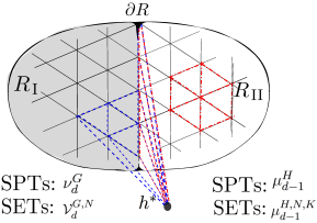 (2)
(2)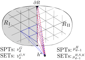
9.2.1 Trivial product state and lattice Hamiltonian
We can consider a total trivial product state wavefunction, where specifies the group element in a symmetry group and its assignment to a local site on a regularized D spatial manifold , the wavefunction has its coefficient: Its wave state-vector in the Hilbert space is:
| (9.17) |
which we can properly normalize to have . Note that has a tensor product structure, here is the site index for some site distributed around the spatial manifold . To see that the state-vector is a trivial product state, we notice that it is indeed a tensor product of on each site , where sums over all group element bases. The Hilbert space on each site is with a Hilbert space dimension spanned by . The total Hilbert space is also a tensor product structure:
Consider the site index , we can write down the exactly soluble Hamiltonian whose ground state is :
| (9.18) |
Here is a local operator on each site , and is an equal-weight sum of all states of all group elements on each site. Thus is proportional to a constant matrix in the group element basis acting on each site. Thus we construct a trivial product state and lattice Hamiltonian for a trivial insulator with a finite energy gap.
9.2.2 Short-range/long-range entangled states and SPT/topologically ordered/SET lattice Hamiltonians
Now we consider a gapped short-range or long-range entangled states for an anomaly-free Hamiltonian on a closed space that is well-defined in D spatial lattice. We can consider either (1) a -SPTs for a cocycle in Sec. 9.1.1, or (2) an -gauge theory with intrinsic topological order for a cocycle in Sec. 9.1.2, or (3) a SETs prescribed by for a cocycle in Sec. 9.1.3.
The SET state in Sec. 9.1.3 is the most general containing all other cases by eqn.9.1.3, thus we focus on the SETs below. For a nontrivial non-product state wavefunction of SETs, we define a particular wavefunction coefficient on a closed space as:
| (9.19) |
where are a set of site () and link () variables on , for and . Conventionally is a phase, except that we set as zero if and only if any face of its simplex violates . The is fixed and assigned to an additional fixed point outside . There are link variables from any site on to . Given a wavefunction input parameter , to determine the wavefunction , the only input data we need are these two:
We only need to provide another input data , as a link variable connecting between a particular site to . Any other variables are determined by a zero flux condition through any closed loop , namely: . Here is a product over all simplices assigned with cocycles. The zero flux condition through any closed loop constrains that the wavefunction has a trivial holonomy around any cycle of the closed manifold. Thus, we only generate a unique ground state so far. (We will comment how to generate other ground states with nontrivial holonomy for topological orders/SETs later.) This ground state as a vector in the Hilbert space is, up to a normalization:
| (9.20) |
The has a tensor product structure,
Now we construct an exactly soluble Hamiltonian for the above gapped ground state as
| (9.21) |
The first term, acts on the wavefunction of a constant-time slice through each vertex in the space by lifting the initial state through an “imaginary time” evolution to a new state with a vertex via
| (9.22) | |||
| (9.23) | |||
We define operator above by its operation on a state-vector . Under the operation, the group element assigned to as has evolved to as , the link element assigned as has evolved to , and has evolved to .

In any dimension, we can construct -simplices (that can be of irregular sizes) as a lattice to fill the space. More explicitly, consider for example a 2+1D SETs, acts on a Hilbert space state-vector for a 2D spatial lattice system in Fig. 22, centered at the vertex and its six nearest-neighbored links:
| (9.24) |
We design the term as the zero flux constraint on each face / plaquette. More explicitly, consider a face (in Fig. 22) with three vertices (assigned ) and three links (assigned ), the acts on the corresponding state vector as
| (9.25) |
The is a Kronecker delta which gives 1 if is trivial in ; thus, the flux through the face is zero. The gives 0 otherwise. Even for SETs, the explicit zero flux condition is reduced to
the same as pure -gauge theory of topological order. For SPTs with a nontrivial but a trivial , the zero flux always manifests as . Some more remarks on the system are given as follows:
-
1.
All and have mutually-commuting and self-commuting nice properties. In principle, our model is an exactly soluble lattice model.
-
2.
Since the SPTs always satisfies the zero flux on every face , we can simplify the Hamiltonian without the term: The additional term in eqn. (9.21) for SETs and topological orders imposes the zero flux constraint at low energy. However, at high energy, at the cost of an energy penalty, the zero flux condition does not hold at those faces with energetic anyon excitations. The anyon excitations are created at the end points of extended operators (e.g. line operators in 2+1D). See also Remark 8.
-
3.
Hilbert space: The Hilbert space on each site is with a Hilbert space dimension spanned by for . The Hilbert space on each edge is with a Hilbert space dimension spanned by for . For our lattice Hamiltonian eqn. (9.21), the total Hilbert space is a tensor product structure:
(9.26) When we limit to a symmetric -SPT, with , we have a tensor product defined on sites. When we limit to a gauge group -topological order, with , we have a tensor product defined on links. Naively, one may ask that isn’t that “the discrete gauge theory description of topological order has no tensor product Hilbert space ?” The answer is that the gauge theory description of topological order for our Hamiltonian eqn. (9.21) only occurs at the lowest-energy ground states, when as zero flux on every face. For those ground states of topological order, indeed, the Hilbert space is not a tensor product, , due to the requirement of projection constrained by . Thus, our Hamiltonian as a local bosonic lattice model at higher energy contains more than a discrete gauge theory. The same argument holds for SET states.
-
4.
Gauge and global symmetries for Hamiltonians: The Hamiltonian in eqn. (9.21) is apparently invariant under the -gauge eqn. (9.7) and -global symmetry eqn. (9.8) transformations. For SETs and SPTs, each individual of and terms is both -gauge invariant and -global invariant. On the other hand, for a topological order of gauge group without any global symmetry (i.e. ), the individual is not gauge invariant. For example, under a local gauge transformation applied on the vertex , it transforms . If a local gauge transformation is applied on a neighbored vertex next to , then is invariant. However the overall is gauge invariant.
-
5.
Gauge and global symmetries for wavefunctions: For the SET state vector of eqn. (9.20), we can apply symmetry transformations on either the wavefunction coefficient or on the basis ; the two transformations are equivalent by an inverse transformation on another. Thus, we focus on the transformations on the wavefunction .
If is nontrivial, then we have either SPTs or SETs. It is easy to check that the cocycle is both gauge and global symmetry invariant under -gauge eqn. (9.7) and -global symmetry eqn. (9.8) transformations. Thus, apparently, the wavefunction
is gauge and global-symmetry invariant under transformations of eqn. (9.7) and eqn. (9.8).
If is trivial and the gauge group is nontrivial, then we have a pure gauge theory with topological order. The reduced inhomogeneous cocycle alone is not gauge invariant, the wavefunction is not gauge invariant, either. Even the ground state vector is not gauge invariant, and is not gauge invariant up to a phase. Namely, each wavefunction obtains a different phase that depends on the input and gauge transformation , i.e. . We define such a gauge transformed state vector as . However, as long as any physical observable is strictly gauge invariant as we show below,191919 Recall that the gauge transformation can be implemented on the basis (a vector in the Hilbert space) or on the wavefunction (effectively a “covector”). The operator can be also implemented either on the basis as or on the wavefunction In either case, we obtain the same consistent result for acting on the state vector as in eqn. (9.28). the theory is well-defined. We find that is indeed gauge invariant,
(9.27) where we have considered a generic operator defined by its operation on :
(9.28) with generic coefficients.
-
6.
Wavefunctions and their independence of input and : Consider a wavefunction on a closed space defined in eqn. (9.19).
SPT wavefunction is independent of the input choice . Namely, changing to(9.29) Here we use the fact that is -global symmetry invariant in the second equality. This proof requires the use of a -cocycle condition, and we will show a complete proof in Sec. 9.2.4, even in the presence of a gapped boundary/interface. We also use that due to the property of a homogeneous cocycle in the third equality. One quick way to visualize this proof eqn. (9.29) is that the ratio yields a term equivalent to a product of coboundary terms; fortunately the overall coboundary terms on a closed space must cancel out to be 1.
Topological order and SET wavefunction can be defined in such a way that it is independent of the input and . It is easier to prove that if we design and evaluate eqn. (9.19) in terms of homogeneous cocycles. Below we show that replacing and , with a slight reordering of vertex indices and branch structure for our convenience, the is still invariant:(9.30) (9.31) The becomes that of topological order if we set all for the trivial . The proofs in eqn. (6) and eqn. (6) again require the use of a -cocycle condition and the property of a homogeneous cocycle.
-
7.
Local unitary transformation and the Hamiltonian: We can define a unitary transformation as
(9.32) We can view that the above is a complex phase determined by local input data that are given within a local -simplex. Since the sends the input state to the same output state. The overall phase is determined by , which is a product of phases assigned to each -simplex.
For SPTs, it is
(9.33) For SPTs, actually this is a local unitary transformation (LUT), because this is formed by a local circuit of many independent on each local simplex. Overall is a unitary diagonal matrix acting on the full Hilbert space with diagonal elements assigned with distinct phases. Under this LUT, the SPT’s is deformed to of eqn. (9.17) as a trivial product state. However, such a LUT locally breaks the global symmetry of SPTs, because each is not -invariant with a fixed . The LUT can deform such a short-range entangled state of SPTs to a trivial product state at the cost of breaking its global symmetry.
The SPT Hamiltonian (without the term) can be rewritten as
(9.34) The is an equal-weight sum of all states for all on each site.
For topological orders/SETs, the defined in eqn. (9.32) is not unitary for the total Hilbert space , because is defined to be when a closed loop . We can artificially redefine to design those zero terms to be by hand, and make a new unitary matrix. For example, one such unitary deformation sends to
where is a projection operator imposing the zero flux condition through a closed loop as , and projects out any state. However, this final state is very different from a trivial product state, e.g. . Regardless of how we design a unitary matrix, we cannot deform the ground state of topological orders/SETs to a trivial product state through any local unitary transformation. This reason is due to a super-posed extended loop states as ground states of intrinsic topological orders are highly long-range entangled — their information encoded in the projection on the zero flux condition is incompatible with a trivial product state. The LUT cannot deform a long-range entangled state to a trivial product state. Thus topological orders/SET Hamiltonian cannot be rewritten as , for any unitary and for some local Hamiltonian whose ground state is a trivial product state.

Figure 23: An example of line operator acts along the blue dashed line. The product of spans along all the vertices on the blue dashed line. One of the most generic operators on this lattice centered at a vertex acts on a local Hilbert space of 7 -vertices and 12 -links on a shaded honeycomb region, thus it acts on a Hilbert space of dimensions . -
8.
Degenerate ground states with holonomies around non-contractible cycles: So far we focus only on a ground state that has no holonomies around non-contractible cycles, and that can be deformed to a trivial product state. However, for gauge theories of topological orders and SETs, we have distinct degenerate ground states when the spatial topology is nontrivial (e.g. a 2D spatial torus ). Start from , we can generate other degenerate ground states by inserting extended operators as holonomies around non-contractible cycles. Without losing generality, let us consider a 2+1D system; we have generic line operators in a 2D spatial torus with coordinates and . We can fully generate distinct ground states spanning the dimensions of Hilbert space on by
(9.35) Here in means that the line operator has a cycle around , so the means a series of vertices spanning around the -cycle, for example along the blue dashed line in Fig.23. The is a shorthand expression , which acts on the honeycomb shaded region in Fig.23. Examples of include the and terms. For example, for a toric code [60] on a torus, the expression for degenerate ground states boils down to
where and are the rank-2 Pauli matrices. The product is along the line operator. The are integer mod 2 values, with are four distinct ground states. Moreover, a generic does not need to commute with and , and it can violate the zero flux condition of Remark 2. Thus such a can create anyon excitations that cost higher energy.
We can easily generalize the above discussion (2+1D) to any spacetime dimension.
9.2.3 Anomalous symmetry-preserving gapped boundary/interface of bulk SPTs and SETs
Continued from Sec. 9.2.2, we develop further to formulate a lattice wavefunction and Hamiltonian for topological phases with gapped boundaries/interfaces. We first focus on a bulk -SPTs on an open manifold while the gapped boundary has an anomalous -SPTs that cannot exists without an extended bulk, via a group extension in Sec. 9.1.4. Along the way, we comment how to easily generalize to a bulk with SETs.
-
•
Wavefunction: For wavefunction, we can simply adopt the -SPT limit of eqn. (9.19) as defined first on a closed space of -spatial dimensions. The is again some fixed value outside the . We would like to keep the degrees of freedom on each site with Hilbert space dimensions on the gapped left region , and extend the site’s Hilbert space dimensions to on the gapped right region as well as on the interface ( up to an orientation). We denote the group element in assigned along as . We also extend the Hilbert space dimensions of from to , and we choose . The modified wavefunction defined on is
(9.36) (9.37) (9.38) (9.39) (9.40) where we have split the above -coboundary in eqn. (9.36) into -cochains in eqn. (9.37). We define
(9.41) Notice that is simplified to no dependence on because those that depend on are pair cancelled out due to overlapping on the same -simplex with opposite orientations . From eqn. (9.38) to eqn. (9.39), the notation “” means that we do a local unitary transformation (LUT) to deform to a gapped trivial product state without breaking any symmetry. Thus, the simplified nontrivial wavefunction only resides on and as .
For example, more explicitly in 2+1D,
(9.42) Here the shorthand depends on the ordering of each assigned simplex. We see that those that do not depend on can be deformed to a gapped trivial product state by local unitary transformation without breaking any symmetry (again, we denote the procedure as “” ), because the homogeneous cochain satisfies . Thus keeping only but removing other , we obtain the last simplified equality. In generic dimensions, we have eqn. (9.40).
-
•
Lattice Hamiltonian: The Hamiltonian for the above gapped ground state has the same form in the bulk region as in eqn. (9.21). However, we need to modify the boundary term on . The first term on the boundary acts on the wavefunction of a constant-time slice through each vertex in the space by lifting the initial state through an “imaginary time” evolution to a new state with a vertex via
(9.43) (9.44) (1)
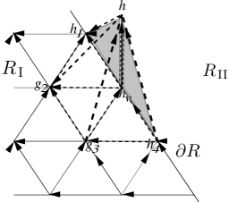 (2)
(2) 
Figure 24: (1) We consider a -SPTs on the spatial region with a lattice. We set a trivial vacuum on the spatial region , and the gapped boundary of -anomalous SPT on the boundary . The Hamiltonian acts on the state and is given in eqn. (9.45), which sends to a new state with a phase. (2) Now consider a -SETs on the spatial region lattice with a gapped boundary anomalous SETs, the Hamiltonian is given in eqn. (9.49). More specifically, the effective 2+1D Hamiltonian term along the 1+1D gapped boundary , shown in Fig. 24 (1), is written as:
(9.45) The term imposes trivial - and - holonomies for the contractible loop. But here does not play any role for SPTs, because SPTs always have trivial holonomy regardless the loop is contractible or not.
-
•
More generic bulk/gapped boundary SET wavefunction and Hamiltonian: We can consider more generic bulk SETs and boundary anomalous SETs as in Sec. 9.1.4 Remark 4 — a bulk SETs with global symmetry and gauge symmetry via , and a boundary anomalous SETs with global symmetry and gauge symmetry via where . This also implies . The generic wavefunction is
(9.46) where Its Hamiltonian has the same form in the bulk region as in eqn. (9.21). But we need to modify the boundary term on to
(9.47) (9.48) Here and are some modified link variables that may have and variables inserted.
The term imposes trivial holonomies for the contractible loops; here, plays an important role to constrain ground states of SETs. The bulk imposes trivial - and -holonomies for the contractible loops. The boundary imposes trivial -, - and -holonomies for the contractible loops. Similar to eqn. (9.25), the bulk constrains that , and the boundary constrains that on each state vector associated to a 2-simplex triangle.
For example, more specifically, an effective 2+1D Hamiltonian term along the 1+1D anomalous SET gapped boundary , shown in Fig. 24 (2), is written as:
(9.49) Here and are aimed at emphasizing that they are obtained via the epimorphism . The and are aimed to emphasize that they are obtained via the monomorphism . Since is a normal subgroup inside , previously we have been abbreviating for .
In the next section, we analyze the symmetry-preserving property of such a gapped boundary system in Sec. 9.2.4.
9.2.4 Proof of the symmetry-preserving wavefunction with gapped boundary/interface
Follow the setup in Sec. 9.2.3, here we rigorously prove that the wavefunction eqn. (9.40) of a bulk -SPTs on an open manifold while the gapped boundary has an anomalous -SPTs via a group extension (in Sec. 9.1.4). See Fig.25 for a geometric illustration for the proof.
We would like to interpret that the spatial bulk have two sectors and , while the whole closed space is .
The SPTs of symmetry group is on the side, a trivial vacuum is on the side,
while the gapped interface () between the two phases is symmetry-enhanced to .
This gapped interface can be viewed as a gapped boundary for the bulk SPTs.
Under the construction
of cocycle splitting,
below we can have an exact
global symmetry transformation acting along the gapped interface, together with an exact
global symmetry transformation acting on the gapped left region , and no symmetry transformation on the trivial right region .
We consider the following setup:
(1) We assign a Hilbert space dimension on each site along the interface
between the and the regions, while the
region of the SPTs has a Hilbert space dimension on each site.
(2) We require the dimension of Hilbert space on the additional site assigned with outside has a Hilbert space dimension . We also have an additional virtual site assigned with for , such that , and
We also set that the site has a
Hilbert space dimension . The condition (2) is important in order
to split the cocycle on the region that touches the interface.
(3) We consider the algebraic structure preserving map from to
with , the same map of . The symmetry transformation
sends when the dimension of Hilbert
space is on the site . The symmetry transformation sends when the Hilbert space dimension is on the site .
The exact global symmetry transformation on the left region and the exact global symmetry transformation along the interface yield global phases to the wavefunction, and the global phases need to cancel out to 1. The cancellation of global phases of -symmetry and -symmetry transformations may be viewed as anomaly-free for the whole bulk and the interface. The wavefunction is only symmetry-invariant if we consider the whole system together.
Now consider the group manifold that has the left () sector of group and the right sector of a trivial vacuum, and all sectors can be lifted to the larger group . Again we set that . In general, we can easily generalize our result to any dimension. Without losing generality, let us take a specific example in 2+1D. And let us consider the 2-dimensional space lattice defined on a 2-sphere . The can be regarded as two 2-disks glued together along the boundary. Let us call the two disks as assigned with on each site, and assigned with on each site. Along the boundary, we assign on each site. The wavefunction on the whole surface is evolved from an additional point assigned . Thus the wavefunction can be determined by assigning the 3-cocycle into this spacetime volume of the ball (whose center is and whose spatial sector is ).
For SPTs, we use the homogeneous cocycle denoted and cochain , and we follow the wavefunction in eqn. (9.42). Here we arrange the wavefunction separated into a few parts:
| (9.50) |
Again there are orientations for each term.
Below we verify that the wavefunction is invariant under the global-symmetry transformation . It means that we can show the is equal to
| (9.51) |
We also denote the change in . The above shows the symmetry transformation acts on the wavefunction. Conversely, we can consider the equivalent dual picture that the symmetry transformation acts on the state vector in the Hilbert space. Either way leads to the same conclusion. Since
| (9.52) |
we need to show that the factor in the bracket is 1 to prove the global symmetry preservation. The -symmetry on the region must be able to be lifted to some -symmetry on the whole regions including the interface , based on the fact that is surjective. We remind the readers that , . Namely, it is effectively the -symmetry transformation on the whole system.
(1)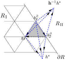 (2)
(2)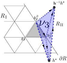 (3)
(3) (4)
(4)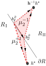 (5)
(5)
In region , the wavefunction change can be simplified further based on a -cocycle condition,
| (9.53) | |||
| (9.54) |
Here for convenience, let us denote as a link connecting two vertices and , where two vertices are assigned with and respectively. Notice the 3-cocycle which contains a link is cancelled out, because there exists a neighbor term which shares the same link and which contributes the same factor with opposite orientation thus opposite sign for . The only subtle type of terms, that survives and that requires further analysis, is which contains a link with two vertices on the interface . If we approach from the region , we see that
| (9.55) |
All the terms on the right-hand side cancel with some other terms in the product which share the same links connecting and on the same region , except that term that touches the link . We would like to split 3-cocycle that touches the link into 2-cochains :
| (9.56) |
We shall consider all such splitting terms along the interface. As an example, for the 1+1D interface on a spatial ring with a total number of sites and links () where (mod ), we obtain:
| (9.57) | |||||
The first is based on eqn. (9.2.4) on a ring. For the second equality, we use the fact that cancels out on a closed ring. Combined with the fact that homogenous cochain does not change under symmetry transformation if inputs do not contain , due to that the homogenous cocycle satisfies , so far we derive that
| (9.58) |
We can also see that the remaining part of wavefunction is , where the inverse with is due to the opposite orientation accounted from the other side . Its symmetry transformation becomes:
| (9.59) |
Thus the phases in eqn.(9.58) and eqn.(9.59) cancel perfectly, and the whole wavefunction is invariant under the symmetry transformation:
| (9.60) |
In Fig.25, we show a neat geometrical way to understand the symmetry-transformation phase cancellation for the symmetry invariance. For any higher -dimensional spacetime, we can give the same proof by replacing in eqn.(9.58) and eqn.(9.59) with . It is easy to confirm that our proof on symmetry-preserving gapped interface holds for any higher-dimensional generalization (q.e.d).
We can apply a similar proof for the global-symmetry-preserving property of the SET version of wavefunction eqn. (9.46) to show
| (9.61) |
To prove this, we may regard that where . Similarly, , we find that . Regardless the branch structure for vertex ordering, we can convert the symmetry transformation, from acting on the left of the group elements to that acting on the right of group elements. This trick can facilitate the proof that the SET wavefunction is invariant under global symmetry, even in the presence of gapped interfaces.
9.2.5 More Remarks
Here are a summary and some more remarks:
-
1.
Global enhanced -symmetry invariant: We have shown that the SPTs wavefunction on a whole system is invariant under -symmetry transformation in the bulk together under -symmetry transformation on the interface . The symmetry transformation is fixed by , and we may view that the symmetry is enhanced to for the whole system.
-
2.
Global -symmetry on the boundary/interface: Under the construction for -bulk SPTs and an anomalous boundary -SPTs, the is trivial in the bulk as for . How about -symmetry transformation on the interface? It is easy to check there is no local -symmetry on the interface, since for arbitrary local transformation on each site . However, below we can prove that there is a global -symmetry applying on the boundary/interface, namely
(9.62) Proof: Without losing generality, consider the 1+1D boundary of 2+1D SPTs. We see that
(9.63) where in the last equality we use the fact of 3-cocycle splitting and so
(9.64) -
3.
Gauging SPTs to SETs: Since there is a global -symmetry on the boundary/interface, we can partially or fully gauge this -symmetry. We can also gauge a normal subgroup of the global symmetry of -SPTs — however, to gauge in the bulk we also need to gauge the for the anomalous -SPTs on the boundary/interface. By gauging the normal subgroups and , this gives rise to SETs of Sec. 9.1.4 Remark 4.
-
4.
Degenerate ground states and holonomies for the boundary anomalous SETs: If the gapped boundary is on a compact space with nontrivial cycles, there can be nontrivial holonomies for the gapped boundary anomalous SETs. For example, for a 2+1D SPTs on a 2-disk and its 1+1D anomalous SETs on a 1-circle , or, for a 3+1D SPTs on a solid torus and its 2+1D anomalous SETs on a 2-torus , their nontrivial boundary holonomies imply the ground state degeneracy (GSD). We will explicit compute such GSDs for some examples in Appendix D, such as in Sec. D.4.1 and in Sec. D.10.1.
-
5.
Gapped interfaces by folding trick: Again based on the folding trick, we can construct a wavefunction and lattice Hamiltonian of gapped interfaces between two topological phases in Sec. 9.1.5, and we still can prove the symmetry-preserving wavefunction.
10 Conclusion
Some concluding and additional remarks follow:
-
1.
We provide a UV complete lattice regularization of the Hamiltonian and path integral definition of gapped interfaces based on the symmetry-extension mechanism, partly rooted in Ref.[40]. Presumably, some of other phenomenon studied in Ref.[40] could also be examined based on our lattice regularized setting.
-
2.
The anomalous non-onsite -symmetry at the boundary indicates that if we couple the -symmetric boundary to the weakly fluctuating background probed gauge field of , there is an anomaly in (in the same language as in particle physics and high-energy theory) along the boundary. The -anomaly can be a gauge anomaly (e.g. for an internal unitary -symmetry), or a mixed gauge-gravitational anomaly (e.g., for a -symmetry that contains an anti-unitary time reversal symmetry ). The key ingredient of our approach is based on the fact that certain non-perturbative global anomalies in at the boundary become anomaly-free in , when is pulled back to (see Sec. 4.5).
-
3.
Given some bulk -SPT states, our formulation finds their possible -symmetry-extended and -symmetry-preserving gapped boundaries, via a suitable group extension .202020 To make a comparison, we remark that Refs.[26, 61, 62, 63] show a related physics by starting from a given anomalous boundary field theory, and finding the possible bulk TQFT. To construct an -symmetry-extended gapped boundary, we actually require a weaker condition on the group extension that may be a finite group or a continuous group, in any bulk dimension 1+1D. To construct a -symmetry-preserving topologically ordered gapped boundary, we further require a stronger condition on the group extension that is a finite group, in order to have a boundary deconfined -gauge theory, for a 3+1D bulk and above.
-
4.
When , and are finite groups, we can prove that there always exist -symmetry extended gapped boundaries (in any bulk dimension 1+1D) and there always exist -symmetry preserving gapped boundaries (for 3+1D bulk and above). The gauge anomaly associated to a finite symmetry group must be a non-perturbative global anomaly. The cohomology/cobordism group of a finite only contains the torsion part, which indicates the non-perturbative anomalies.
We believe that the argument remains valid, even when and are infinite continuous compact groups, but remains a finite group. In this case, the boundary dynamics still yields a deconfined -gauge theory, given that the bulk dimensions are larger or equal to 3+1D (see Sec. 6). (When the bulk is 2+1D, we comment in the next remark.)
When is a continuous group for the bulk -SPTs, the boundary could have both perturbative anomalies (e.g. captured by a 1-loop Feynman diagram), or non-perturbative global anomalies, detected by coupling the boundary to -gauge fields.212121 The free part of the cohomology/(co)bordism group contributes the perturbative anomalies. The torsion part of the cohomology/(co)bordism group contributes the non-perturbative global anomalies. The perturbative anomalies do not offer any symmetry-preserving surface topological orders. In contrast, some of the non-perturbative global anomalies can offer a symmetry-preserving surface topological order as long as our construction trivializes the -anomaly in .222222We demonstrate examples for each case in Appendices: First, a perturbative chiral anomaly of -SPTs in D.19 (with a bulk invariant of even dimensions and an integer ), do not offer a symmetry-preserving surface topological orders but only have a symmetry-enforced gapless boundaries. Other symmetry-enforced gapless boundaries also occurred in [64]. Second, a global mixed gauge-gravitational anomaly on the boundary of 6+1D -SPTs in D.20 (with a bulk invariant ), does allow a deconfined 5+1D surface topological orders.
-
5.
We apply our symmetry-preserving gapped interface construction to the 2+1D bulk and 1+1D boundary. For the 1+1D topologically ordered -gauge theory on the boundary of a finite/continuous group symmetry of 2+1D -SPTs, we find an interesting phenomenon that the 1+1D boundary deconfined -gauge theory states develop long-range orders that spontaneously break the -symmetry (see Sec. 4.8). The 1+1D boundary deconfined and confined gauge theory states belong to the same phase; namely, they are both symmetry-breaking states connected without phase transitions.
Examples include those of a finite gauge group , and a global symmetry containing discrete unitary or ant-unitary global symmetry sectors that can be spontaneously broken. For instance, in Sec. 3.3, and Appendix A.2.4 and D.22, we show that the unitary -symmetry of a 1+1D gauge theory is spontaneously broken, on the boundary of 2+1D -SPTs. In Appendix D.22, we also show that the anti-unitary time reversal -symmetry of a 1+1D gauge theory is spontaneously broken, on the boundary of 2+1D bosonic -topological insulator and -topological superconductor. This is, so far, consistent with the fact that there is no robust intrinsic topological order in 1+1D robust against any local perturbations. 232323However, if we apply our construction for a continuous symmetry group on a 1+1D boundary, due to Coleman-Mermin-Wagner theorem, there shall be no spontaneous symmetry breaking for a continuous symmetry in 1+1D. We may expect to find further interesting new physics. It will be illuminating to address this issue further in the future work.
-
6.
Our approach shall be applicable to obtain gapped interfaces of more generic bosonic and fermionic topological states (other than the fermionic CZX model in Appendix B), including topological states from the beyond-symmetry-group cohomology and cobordism approach (Secs. 6 and Sec. 7). It will be interesting to establish this result with more concrete examples.
Bulk/Interface Dim D.4/5.2: 2+1/1+1D Yes No (-SSB) , D.5: /D Even dim : Yes Yes , D.6/5.3: 3+1/2+1D - Yes D.7: /D Odd dim : - Yes D.8: 3+1/2+1D - Yes D.8: 3+1/2+1D - Yes D.9: 2+1/1+1D Yes No (SSB) , D.10: 2+1/1+1D Yes No (SSB) , D.11: 2+1/1+1D Yes No (SSB) , D.12: 1+1/0+1D No Yes , D.13: 1+1/0+1D Yes Yes , D.14: 2+1/1+1D Yes No (SSB) , D.15: 3+1/2+1D Yes Yes , D.15: d+1/dD Yes Yes D.16: 2+1/1+1D Yes No (SSB) , D.17: 3+1/2+1D Yes Yes , D.18: 3+1/2+1D Yes Yes , D.19: 2+1/1+1D No No (Pert) D.20: 6+1/5+1D - Yes (Global) D.21: 2+1/1+1D - D.21: 2+1/1+1D - D.23: 1+1/0+1D Yes Yes Odd-integer AF spin chain
Table 10: We outline the gapped boundary/interface results obtained in Appendix D. In several cases, we check the validity of two techniques mentioned in Sec. D.3, based on Lyndon-Hochschild-Serre (LHS) spectral sequence technique in Sec. D.3. The “Symmetric Gapped Boundary” column means that the “symmetry preserving gapped interface” is available or not. For a discrete finite , this “Symmetric Gapped Boundary” means the cochain solution is found. “Pert.” means the perturbative anomaly. “-SSB” means the spontaneous symmetry breaking in (e.g. , , etc.). “Global” means the global gauge/gravitational anomaly. “AF” means anti-ferromagnet. The -cocycle for a finite Abelian group with its type indices (written in Roman numerals) follows the notation defined in Ref. [27]. The is the Bockstein homomorphism. -
7.
In Appendix D, we systematically construct various symmetry-extended gapped boundaries for topological states in various dimensions (choosing homogeneous cocycles for SPTs and inhomogeneous cocycles for topological orders), summarized in the Table 10. We can also combine results in different subsections in Appendix D and use the folding trick to obtain the gapped interfaces between topological states.
The previously known gapped interfaces for the toric code and double-semion model can be achieved by certain (gauge-) symmetry-breaking sine-Gordon cosine interactions at strong couplings. The previously known gapped interfaces of 2+1D twisted quantum double models and Dijkgraaf-Witten gauge theories can also be obtained through such a (gauge-) symmetry-breaking mechanism or anyon condensation [65, 66, 67, 68, 69, 70, 71], see Appendix F.1. It is known that there are 2 types of gapped boundaries for toric code, 1 type of gapped boundary for double-semion model, and 2 types of gapped interfaces between toric code and double-semion model [71]. More generally, we systematically show gauge symmetry-breaking gapped interfaces in any dimension, in Appendix F.1, including 2+1D (ours reproduce the results in the previous literature) and the less-studied 3+1D.
However, we can construct other new types of gapped interfaces between toric code and double-semion models via a symmetry-extension mechanism, such as examples given in Appendices D.4’s 2+1/1+1D under , and D.10’s 2+1/1+1D under , and more, etc. Our new gapped interface has an enhanced Hilbert space and to certain degree an enhanced gauge symmetry, the first new type of gapped interface has and the second new type of gapped interface has . Through a symmetry extension mechanism, we can construct new types of gapped boundaries/interfaces in 2+1D, 3+1D and any higher dimensions.242424However, the fate of some of gauge symmetry-extended interfaces turns out to be the same phase as the gauge symmetry-breaking interface. This was later explored in Sec. 7 of [72], where their dual description and equivalence are found.
More generally, our framework encompasses the mixed symmetry breaking, symmetry extension, and dynamically gauging mechanisms to generate gapped interfaces.
-
8.
Fermionic symmetry extension and fermionic spin-TQFT gapped boundaries/interfaces: Previously fermionic gauge-symmetry-breaking 1+1D gapped boundary of 2+1D fermionic TO is examined in [73]. More recently, the 2+1D symmetric anomalous gapped fermionic surface topological order of 3+1D fermionic SPT is examined in [74]. A step toward a possible framework to incorporate these fermionic symmetry-breaking or fermionic symmetry-extension constructions of gapped boundaries/interfaces is pursued in [75].
-
9.
Higher-symmetry extension and higher-gauge theory/TQFT gapped boundaries/interfaces: Ordinary global symmetries can be regarded as the 0-form global symmetries which has a 0-dimensional charged object measured by codimension-1 (thus -dimension) charge operator. Generalized global symmetries [76] include the -form higher global symmetries which has a -dimensional charged object measured by codimension-() (thus -dimension) charge operator. An interesting research direction is to apply the symmetry breaking or symmetry extension method of constructing topological boundaries/interfaces to higher global symmetries, including the higher SPT/SET states. Recent developments along this direction can be found in [61], [77], [78] and References therein.
-
10.
Future application: Gapped interfaces via gauge symmetry breaking or anyon condensations have recently found their applications in topological quantum computation (see [79] and Reference therein for 2+1D bulk systems). We hope that our new types of gapped interfaces via global/gauge symmetry extensions in any dimension have analogous potential applications, for science and technology, in the future.
11 Acknowledgements
J.W. thanks Irina Bobkova, Thomas Church, Tian Lan, Kantaro Ohmori and Pavel Putrov for conversations. J.W. gratefully acknowledges the Corning Glass Works Foundation Fellowship and the NSF. X.-G.W’s research is supported by NSF Grant No. DMR-1506475 and NSFC 11274192. J.W.’s work was performed in part at the Aspen Center for Physics, which is supported by National Science Foundation grant PHY-1066293. The research at IAS is supported by the NSF Grant PHY-1606531 and PHY-1314311.
Appendix
Appendix A Low energy effective theory for the boundaries of CZX model
A.1 Low energy effective theory for
the second boundary of the CZX model –
A 1+1D model with
an on-site -symmetry
In Sec. 3.2, we described a gapped boundary state of the CZX model in which the bulk symmetry is extended to a symmetry along the boundary. The model as described there is gapped in both bulk and boundary, and there is no hierarchy of energy scales: The energy gaps in bulk and along the boundary are comparable.
This is a physically sensible state of affairs in condensed matter physics, but nonetheless one might ask what sort of model would have such a hierarchy of scales. In this section, we will describe several possibilities. As a result, we obtain several pure 1+1D models as the effective boundary theories for the CZX model.
One approach is simply to reduce the coefficient of the boundary plaquette term in the Hamiltonian. In this limit (see Fig. 5), the low-energy degrees of freedom at the boundary are described by three spins per unit cell: , , and a composite spin described by the two spins on the black dots next to and , which are locked due to the projector from the neighboring Hamiltonian.
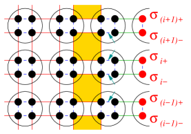
Here, we would like to reduce the boundary degrees of freedom further. To do so, we will consider a slightly different boundary, by omitting the terms in the Hamiltonian and at the same time including some projectors at the boundary. This gives us another description of the second boundary of the CZX model (see Fig. 26). The bulk Hamiltonian of the model is still given by for each complete octagon in the bulk, with addition terms that force the boundary spin ’s to have the same value as the bulk spins connected by the green lines. However, notice that the shaded squares are not complete octagons since the two spins to the right of the shaded squares do not need to be parallel. So the Hamiltonian for the shaded squares needs to be modified:
| (A.1) |
where is given by
| (A.2) |
The above Hamiltonian has a global symmetry. The symmetry is generated by
| (A.3) |
when acts on a boundary site, and by
| (A.4) |
when acts on a bulk site, where , , , and label the four spins on the bulk site. Note that the symmetry is actually a symmetry in the bulk since
| (A.5) |
So here we are actually considering a model with on-site symmetry in the bulk, and the symmetry is promoted to symmetry on the boundary, since
| (A.6) |
The total symmetry generator is given by
| (A.7) |
To see that is invariant under , we first note that is invariant under . Rewriting as , we see that anti-commutes with . also anti-commutes with . Thus is invariant under .
The low energy boundary excitations have a basis labeled by values of the boundary spins:
| (A.8) |
Now, is given by
| (A.9) |
where is the spin state for the four spins connected by a red square in Fig. 26 as determined by , and
| (A.10) | ||||
is the spin state for the four spins connected by a shaded red square in Fig. 26, as determined by .
Under the , is unchanged for . But for , changes and . The extra sign comes from the two uncanceled factors to the right of the plaquette (see Fig. 26 where the factors are pointed out by arrows). Therefore, under the , is changed to
| (A.11) |
So, under the on-site transformation to the whole system, the bulk state changes into itself up to a phase factor:
| (A.12) |
The phase factor depends on the boundary spins and is given by
| (A.13) |
The factors in eqn. (A.13) and eqn. (A.3) cancel each other. Therefore, the effective transformation on the boundary low-energy subspace is given by
| (A.14) |
which is an on-site symmetry if we view as a site. This means that if we view the CZX model as a model with symmetry, it is actually a trivial -SPT state (since the effective transformation on the boundary is on-site and anomaly-free).
To summarize, the original model in the Sec. 3.2 describes a gapped boundary where the boundary plaquette term has the same order as the bulk plaquette term. Now in this Sec. A.1, we reduce the boundary plaquette term to only some newly-introduced projectors on the green links in Fig.26. For certain small or zero , the boundary spins may have no constraint in the whole wavefunction , which can describe a gapless boundary. We have also obtained the effective symmetry transformation on the boundary.
A.2 The low energy effective theory for the fourth boundary of the CZX model – A 1+1D exactly soluble emergent -gauge theory
In the last subsection, we have constructed a boundary of the CZX model that has a symmetry. In this section, we are going to modify the above construction to obtain a boundary that has the same symmetry as the bulk. We will obtain a low energy effective theory for the fourth boundary of the CZX model discussed in subsection 3.4.
A.2.1 The boundary -gauge theory with an anomalous global symmetry
We start with the boundary model obtained in last Sec. A.1, and add qubits described by (see Fig. 27). However, the boundary physical Hilbert space is the subspace that satisfies a local gauge constraint
| (A.15) |
The symmetry generator is the same as before when acting on spins. The symmetry generator acts on the spins as
| (A.16) |
As we have discussed in Sec. 3.4, such a symmetry generator generates an on-site global symmetry, in the -gauge-invariant physical Hilbert space.
Using the effective boundary -symmetry calculated in the last subsection A.1 (see eqn. (A.1)), plus an additional term acting on the new spins, we find that the boundary effective symmetry generator is given by
| (A.17) |
satisfies
| (A.18) |
in the constraint -gauge-invariant subspace. Here we encounter the even-odd lattice site effect again, we assume that the total number of the boundary sites is always even, , including the example that the whole system is on a disk with only a single boundary. We have turned the symmetry in the last subsection into a symmetry.
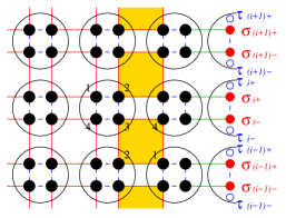
Next, let us include a boundary interaction term . In the following, we will take the limit. In this case, the interaction locks . In the low energy subspace, we introduce
| (A.19) |
that satisfies
| (A.20) |
Now the -gauge constraint becomes
| (A.21) |
The effective symmetry generator becomes
| (A.22) |
After obtaining the effective symmetry on the boundary, we can write down a global symmetric (under eqn. (A.22)) and local -gauge symmetric (under eqn. (A.21)) boundary effective Hamiltonian:
| (A.23) | ||||
This is our fourth boundary of the CZX model discussed in Sec. 3.4, but now it becomes a 1+1D lattice -gauge theory with an anomalous (non-on-site) global -symmetry.
A.2.2 Confined -gauge state – A spontaneous symmetry breaking state
In general, a large in the above Hamiltonian will give us a -gauge confined phase (which will be discussed later in more detail). In the -gauge confined phase induced by a large , we have . In this case, because of eqn. (A.19) and eqn. (A.21), on every site, which reduces two spin and into one spin . This reduces the symmetry transformation into
| (A.24) |
which is a non-on-site (anomalous) -symmetry transformation. Here is a redefinition of for the composite spin. More precisely, due to the gauge constraint , flips the composite spin as and . Since the two spins are locked in the same site, we can also simply define , so that . So in the large limit, the lattice -gauge theory, at low energies, reduces to the boundary of the CZX model constructed in Sec. 3.1. When , the confined -gauge state is a ferromagnetic state, that spontaneously breaks the global -symmetry.
A.2.3 Deconfined -gauge state in 1+1D
The model eqn. (A.2.1) is exactly soluble. This is because in the big Hilbert space before projecting into the -gauge-invariant subspace, the Hamiltonian in eqn. (A.2.1) is a sum of non overlapping local terms: with
| (A.25) |
So the energy spectrum of can be obtained exactly from that of . The -gauge transformation
| (A.26) |
commutes with . So the energy spectrum of in the -gauge-invariant subspace is a subset of the spectrum in the big unconstrained Hilbert space.
In the deconfined state at , and does not fluctuate before we apply the -gauge constraint (i.e. does not fluctuate in the big Hilbert space before projecting into the -gauge invariant subspace, since ). The ground state wave function on each link is , where are the eigenstates of . The gauge-invariant ground states are two distinct holonomy sectors labeled by , explicitly as:
| (A.27) |
Here the coefficient is determined in the same way as eqns.(3.15) and (3.16) with alternating signs set by the gauge-invariant constraint on the ground states .
From the above results, we see that the global charge and the -gauge flux are locked. In other words, the deconfined state has two degenerate ground states on the ring and a finite energy gap. One ground state carries the global charge and no -gauge flux through the ring. The other carries the global charge and the -gauge flux through the ring. Near the end of the next section, we will show that the above deconfined states spontaneously break the global -symmetry, which is another way to understand the two degenerate ground states on the ring.
A.2.4 Deconfined and confined -gauge states belong to the same phase that spontaneously breaks the global symmetry
We note that for the following four spin states , , , and are common eigenstates of and with eigenvalues , , , and .
For , the ground states have a 2-fold degeneracy, which is given by
| (A.30) |
where are eigenstates of with eigenvalues . In order to have the two states as ground states, is constrained to be the function of as .
The energy of the two ground states is . Also for (the -gauge deconfined case) and for (the -gauge confined case). The first excited states also have a 2-fold degeneracy, which is given by
| and | (A.31) |
with energy , which is higher than the ground state energy by at least (note that we have assumed ).
We note that
| (A.32) |
is a common eigenstate of with eigenvalues , and we denote it as or . Similarly,
| (A.33) |
is a common eigenstate of with eigenvalues , and we denote it as or .
A -gauge-invariant ground state (i.e. state) on a ring is given by the tensor product of those and states on the links. First we note that the gauge transformation in eqn. (A.26) is a product of two operators and with an additional sign. The and are eigenstates of those operators. Therefore, we have two -gauge-invariant ground states:
| (A.34) |
up to a proper normalization factor. Note that to get a -gauge-invariant state under eqn. (A.26) we need to match to and to in the neighboring links, as done in the above. However, the two ground states expressed in eqn. (A.2.4) are not symmetric under the global symmetry transformation in eqn. (A.22):
In fact, exchanges and ,
| (A.35) | |||
| (A.36) |
The ground states that respect the global symmetry transformation eqn. (A.22) are the linear combination of eqn. (A.2.4):
| (A.37) |
where the is -symmetry even by , and the is -symmetry odd by .
When , the even/odd symmetric ground states are identical to the even/odd -gauge holonomy sectors of ground states in eqn. (A.27) due to the locking of -charge and -holonomy:
| (A.38) |
When , we have the confined states:
| (A.39) |
up to a proper normalization factor. Below we aim to show that at , namely and , we have the deconfined state with spontaneous -symmetry breaking; at , namely and , we have the confined state with spontaneous -symmetry breaking. We demonstrate a strange property for this system: the deconfined state with spontaneous -symmetry breaking and the confined state with spontaneous -symmetry breaking belong to the same phase. In the next few paragraphs, we explain the meanings of the deconfined and confined phases, and also the meanings of the spontaneous symmetry breaking.
First, we elaborate further on the physical meanings of the deconfined and confined phases. The deconfined phase () here means that the distinct holonomies or loop excitations (namely Wilson lines) can span the large system without causing extra energy. Consider the expectation value of Wilson line operator for some ground state , the goes to some constant (proportional to the net holonomy ) in the Euclidean spacetime, and, thus, obeys the perimeter law instead of the area law [80]. The two ground states with distinct holonomies in our case imply that we are in the deconfined phase, even if the energy spectrum is gapped between the ground states and the first excitations. On the other hand, the confined phase (, ) has the gauge field variable quantum disorder and strong fluctuations in the state . The long-distance lines/holonomies are energy-disfavored. Consider the expectation value of Wilson line operator for any ground state , the exponentially decays to zero in the Euclidean spacetime, thus obeys the area law, thus the phase is confined. The -gauge confined phase for and is a ferromagnetic along the link but anti-ferromagnetic between the neighbored links between spin up and down. There is no phase transition as goes from to for , since the energy gap above the ground state is always bigger than . Thus the -gauge deconfined state for and the -gauge confined state for belong to the same phase.
Second, we elaborate further on the physical meanings of the spontaneous symmetry breaking (SSB) and possible long-range orders. Based on Ref.[81], we know that the SSB in a quantum system does not necessarily mean that its ground states break the symmetry. Traditionally, we identify the symmetry-breaking order parameter and we compute the long-range order correlation functions to detect the symmetry-breaking. The better definition for SSB is based on the Greenberger-Horne-Zeilinger (GHZ) entanglement [82]. Use GHZ form, we can probe the symmetry without knowing the symmetry or the Ginzburg-Landau symmetry-breaking order parameters. Use GHZ form, we can detect the symmetry-breaking hidden in the symmetric ground-state wavefunction.
Indeed, and are GHZ states,
| (A.40) |
Because the -global symmetry operator acting on two states gives rise to the symmetric charge , the following conditions for SSB of symmetry group are satisfied:
-
1.
-
2.
The symmetric GHZ states have the same GHZ entanglement , with , , where are locally distinguishable. In our case, we have and is trivial.
To summarize, the symmetric many-body state has spontaneous symmetry breaking, which implies that the state has a GHZ entanglement. Indeed, we can also show that the SSB here also implies the long-range order, consistent with what we observed in eqn. (3.21) in Sec. 3.3. Defining the gauge-invariant operator which is odd breaking the -symmetry, we find and . Moreover,
| (A.41) |
Thus the -symmetry odd operator detects the long-range correlator of GHZ states, and we demonstrate the SSB through the long-range order. In summary, we show that the deconfined state and the confined state belong to the same phase without the phase transition by tuning the Hamiltonian coupling with the ground state parameter . All values of have the spontaneous -symmetry breaking. This is possible since the -gauge deconfined phase with no spin order has two-fold degenerate ground states with opposite global charge, the same as the ferromagnetic state with spin order which also has two-fold degenerate ground states with opposite global charges.
We remind the readers that the fermionic version of the CZX model is studied in Appendix B. The boundary of the fermionic CZX model with emergent -gauge theory with anomalous global symmetry is detailed in Appendix.C.
One can read Sec. 4 on more general boundaries of SPTs in any dimension.
Appendix B Fermionic CZX model
Consider a square lattice model with each single site endowed with four fermion orbitals, each with eigenstates and of the fermion number operator . Thus a single site has a -dimensional Hilbert space. We may call the single site a “vertex,” and the four individual fermion orbitals in a site “sub-vertices.” In the fermionic model, we have the anti-commutation relation
where can be any local fermion degree of freedom, on the same site or on different sites. Fermion parity operator on each site (with 1,2,3,4 four sub-vertices):
| (B.1) |
Notice that
| (B.2) |
Let us introduce a generator as a product of on the four sub-vertices:
| (B.3) |
where we have used the Jordan-Wigner transformation to express fermion operators in terms of spin operators, for example
| (B.4) |
where refers to a particular ordering of the orbitals (see Fig 28). We have chosen an unusual definition of (instead of the more obvious ), because we want to have a simple form after bosonization.
For any pair of qubits, we set . For each site, we define as the product of such operators over all successive pairs:
| (B.5) |
where . Now we introduce a transformation in each site:
| (B.6) |
The group super-cohomology predicts that there are four distinct fermionic SPTs with symmetry from . The model we will first focus is the one with the second class for . The full classification for four distinct fermionic SPTs with symmetry is from the spin cobordism group ; then, our model here is for .
The fermionic CZX Hamiltonian is essentially the same as the bosonic CZX Hamiltonian:
| (B.7) |
| (B.8) |
Here plaquettes are defined in the bosonic CZX model. acts on the four sub-vertices in a plaquette,
| (B.9) | ||||
and the projection operator acts on a pair of qubits adjacent to a plaquette as
| (B.10) |
We see that, after bosonization, both the Hamiltonian and the symmetry for the fermionic CZX model map to those of the bosonic CZX model. So the ground state of the fermionic CZX model is the same as that of the bosonic CZX model described in Sec. 2.
It is also obvious that since conserves fermion number mod 2 (in fact, conserves fermion number mod 4). So the fermionic CZX model has symmetry generated by and . The ground state is invariant under the symmetry.
Appendix C A boundary of the fermionic CZX model – Emergent -gauge theory with an anomalous global symmetry, and Majorana fermions
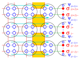
To obtain a boundary of the fermionic CZX model, we start with the boundary model described in Fig. 28. On the boundary, we have qubits described by and fermions described by , where and are Majorana fermion operators, see Fig. 29.

However, we assume that the boundary Hilbert space is not the one generated by and , but a subspace satisfying a local -gauge constraint:
| (C.1) |
where
| (C.2) |
Thus, the boundary is a lattice gauge theory.
The bulk Hamiltonian of the model is still given by for the complete octagons in the bulk, with additional terms that force the boundary qubits to have the same value as the for the bulk fermions connected by the green lines. However, notice that the shaded squares are not complete octagons since the two spins to the right of the shaded squares do not need to be parallel. So the Hamiltonians for the shaded squares need to be modified:
| (C.3) |
where is given in eqn. (A.2). The -symmetry of the system is generated by
| (C.4) |
After the bosonization via Jordan-Wigner transformation on Majorana fermion operators,
| (C.5) |
the above Hamiltonian and the -symmetry map to those of the bosonic model discussed in subsection A.2. So we can use the results there. First one can show that
| (C.6) |
in the -gauge-invariant physical Hilbert space. So generates an on-site global -symmetry. Second one can show that the Hamiltonian is indeed symmetric. Third, one can find the low-energy effective -symmetry on the boundary to be generated by
| (C.7) |
Next, let us include a boundary interaction term and take limit. In this case, the interaction locks . In the low energy subspace, we introduce
| (C.8) |
After the bosonization on the boundary, the above becomes
| (C.9) |
which satisfies
| (C.10) |
Now the -gauge constraint becomes
| (C.11) |
The effective symmetry generator becomes
| (C.12) |
We can write down a symmetric and local -gauge symmetric boundary effective Hamiltonian:
| (C.13) | ||||
which is identical to the effective boundary Hamiltonian (A.2.1) in Appendix A.2.
Note that all the low-energy excitations at an energy scale much less than are purely bosonic. So the fermionic CZX model has a boundary that can be identified as a boundary of bosonic CZX model, stacking with a fermionic product state. This implies that the ground state of the fermionic CZX model can also be viewed as a bosonic -SPT state, stacking with a fermionic product states.
Appendix D Symmetry-extended gapped boundaries/interfaces: Comments, criteria and examples
In this section, we aim to show many systematic examples of -topological states, such that we can construct -gapped boundary/interface through the symmetry extension mechanism, based on a group homomorphism (a surjective epimorphism) by a short exact sequence
| (D.1) |
In Sec. 4.4.1, we considered the mathematical set-up that -cocycle is trivialized in based on homogeneous cocycles , in order to consider SPT states. In this Appendix D, instead, we set-up the mathematics based on inhomogeneous cocycles , for the convenience of notations (which becomes more transparent later) and for more general topological phases (SET states and intrinsic topological orders).
The plan of this Appendix D is the following. In Appendixes D.1 and D.2, we will give an overview of the set-up of problems on the boundaries/interfaces. In Appendix D.3, we show that the Lyndon-Hochschild-Serre (LHS) spectral sequence criteria, are helpful to analytically derive some split -cochains that can trivialize certain -cochains (that can be -cocycles) of one higher dimension. The advantage of this LHS approach, compared to Sec. 5, is that we can obtain some analytic split -cochains.252525 Note that Sec. 5’s approach can only suggest the possible for a given and a given -cocycle, but Sec. 5 cannot provide any analytic -cochain easily. However, the drawback of this LHS approach is that, in a few cases, the -cochains may not always be the -cocycles that we hoped for (standing for nontrivial -topological phases) but -coboundaries (standing for a trivial vacuum). Nevertheless we can still produce many valid successful examples through Appendix D.3’s LHS approach shown later in Appendix D. For all the examples given from D.4 to D.23, all that we aim to provide are the data of the inhomogeneous -cocycle and its trivialization by finding the split -cochain .
D.1 Symmetry Extension Setup: Trivialize a -cocycle to an -coboundary (split to lower-dimensional -cochains) by lifting to a larger group
We switch to using the inhomogeneous version of -cocycles and -cochains for the convenience of notations. The inhomogeneous version is more general and suitable even for gauge theories with nontrivial holonomies around non-contractible cycles. Moreover, we can convert between and based on the well-known relation given in eqn. (9.1.3). We can develop their path integrals, lattice Hamiltonians and wave functions suitable for many-body quantum systems as in Sec. 9.
The setup of symmetry-extension eqn. (D.1) for inhomogeneous cocycles goes as follows. By pulling back a -cocycle back to , it becomes an -coboundary . Formally, we mean that a nontrivial -cocycle
| (D.2) |
becomes a trivial element (a coboundary) when it is pulled back (denoted as ∗) to
| (D.3) |
This trivial element means a trivial group element in the cohomology group , or a coboundary for the coefficient. The above variable (or ) in the bracket is a shorthand of many copies of group elements in a direct product group of (or ). More precisely, we rewrite the above in terms of splitting a inhomogeneous -cocycle:
| (D.4) |
Because of the property of the -module for the cohomology group of cocycles, we impose that for contains only a unitary group element, and for is an anti-unitary group element in such as an anti-unitary time-reversal symmetry group.
We call this approach “symmetry extension” (or colloquially “symmetry enhancement”), because is a larger group mapping surjectively to . For quantum many-body systems, the dimension of Hilbert space is enhanced from a per degree of freedom in the bulk to a larger per degree of freedom on the boundary.
Here we provide some useful information of the cohomology group of that may be used later:
| 0 | ||||
| subgroup | quotient group | |
|---|---|---|
| (center) | ||
| No | No | |
| No | No | |
| No | No | |
| No | No | |
| subgroup | quotient group | |
|---|---|---|
| (center) | ||
We write the order-8 dihedral group as
generated by and . We write the order-8 quaternion as
so that each element in we can write uniquely as , where and . For , we can identify them as the well-known notation as .
For notation convention, we use the additive notation to denote the trivial group if all groups are finite Abelian groups such as in . We use the multiplicative notation to denote the trivial group if some group is non-Abelian such as in .
D.2 Symmetry-extended gapped interfaces
Consider the interface (i.e. domain wall) between two sides of phases labeled by groups and respectively. The two sides of phases could be either both SPTs, both SETs or both topological orders. Below we present various systematic constructions for gapped interfaces. The gapped boundary of can be regarded as a gapped interface between a -topological state and a trivial vacuum.
D.2.1 Symmetry-extension and the folding trick: Trivialize a -cocycle to an -coboundary by splitting to lower-dimensional -cochains
Importantly the previous formulation of gapped boundary is also applicable to formulate the gapped interface, by using the folding trick. The strategy is that, by replacing the in Sec. D.1 to , then we can determine the gapped boundary between and the vacuum, via trivializing a -cocycle to -coboundary by splitting to lower-dimensional -cochains. The surjective group homomorphism is given by
We can rewrite the above in terms of splitting an inhomogeneous -cocycle:
| (D.5) |
Here is a shorthand of with each element in . Generally is a cocycle in the cohomology group . Künneth theorem shows us that there exists a particular form of cocycle , obtained from and . Now, we see that the -symmetry action only acts on , while the -symmetry action only acts on . By folding and to two different sides of the -gapped boundary, we obtain an -gapped interface.
D.2.2 Append a lower-dimensional topological state onto the boundary/interface
For all the previous setups, we actually pick a trivialization of the pullback of the -cocycle to . The possible trivialization choices differed by a class in physically imply that we can further append lower dimensional gapped topological states (that are well-defined in its own dimension) onto the boundary or the interface. (See also Sec. 8.2 for a discussion.) In general, it could be a SET of -dimensions labeled by an -cocycle with -site and -link variables:
| (D.6) |
and described by , with a total projective symmetry group , a gauge group , and a global symmetry group . The cocycle obeys the cocycle condition: . In different limit choices of and , the topological phases of include SPTs, topological orders and SETs.
The proper choices of and on the boundary are also constrained by the choices of and in the bulk. We will leave this issue as a case-by-case study.
D.3 Criteria on trivializing the -cocycle in a larger group :
Lyndon-Hochschild-Serre spectral sequence
We would like to provide a systematic way to determine the possible trivialization of the -cocycle in by lifting to a larger group , based on the setup of the Lyndon-Hochschild-Serre (LHS) spectral sequence. The question we would like to address here is that
“Given , how can we analytically obtain the split -cochain that satisfies that for some -cocycle ?”
An answer goes as follow.
For , with acting trivially on ,262626
If is contained in the center of , it implies acts trivially on .
there is a spectral sequence
with:
(a) .
(b) The differential is defined as a map : . We have at .
We focus on the differential of the page in the LHS spectral sequence
| (D.7) | |||
| (D.8) |
in particular
| (D.9) |
If we want to trivialize the -cocycle , we can look for a larger group , where for some . The turns out to provide the following nice property. The image of the differential provides elements of , such that all such elements are guaranteed to vanish to be trivial as a coboundary in . In other words, every element in the image of the map is guaranteed to be trivial in .272727 Namely, the image of the map is guaranteed to be contained in the kernel of the inflation map from to . J.W. gratefully acknowledges Tom Church and Ehud Meir for illuminating the spectral sequence method [83, 84]. Given , if is killed by (namely, is in the image of ), in other words , then becomes a coboundary in . We have
| (D.10) |
or, more precisely,
| (D.11) |
where is determined by the differential and the map
| (D.12) |
The is a function that relates to a cocycle
| (D.13) |
If we know the data of are given by the pair and , we can propose the .282828For example, we can write as a function F as . For many examples shown in this Appendix D, we find that a candidate form of is . Notice that is in . The claim is that there exists the map where every -cocycle in the image of map is an -coboundary that can be split to lower-dimensional -cochains in .
By writing the group element in terms of a pair as , we can write down the further precise relation
| (D.14) |
Such a construction of so that is a coboundary in , from the LHS spectral sequence. This means that some -cocycle can be split to lower dimensional -cochains. However, we emphasize that some obtained may be already a -coboundary and may not be the specific non-trivial -cocycle that we originally aimed to trivialize. We will show in Appendix D (from D.4 to D.23) how this LHS spectral sequence approach can help in constructing some examples, but not necessarily other examples.
D.4 2+1/1+1D Bosonic
Consider the example where , and , and denote them under . The twisted 3-cocycle is
| (D.15) |
with and . To have a nontrivial 3-cocycle, we set . This cocycle is equivalent to with a cup product form of , in . The here is a -valued 1-cocycle in on the spacetime complex . For a discrete finite , the principal -bundle and the flat connection are effectively the same. Here we consider , so in this context, we can view the nontrivial SPTs detectable by the principal -bundle and the flat -connection
We find that the analytic 2-cochain
| (D.16) |
splits 3-cocycle. Alternatively, we can choose with .
Furthermore, we find LHS technique in Appendix D.3 works successfully. For LHS technique of Appendix D.3, we look for:
| (D.17) |
| (D.18) |
Because this maps to , the can be a base of . We find that another 2-cochain that splits 3-cocycle is
| (D.19) |
For ; ; ; . The group elements in satisfy
We would like to check that .
| (D.20) | |||
| (D.21) |
which is true. (Actually, both and work to trivialize 3-cocycle.) We can rewrite . If we write in terms of , then .
If we consider the bulk to be fully gauged topologically ordered state, this becomes a gapped boundary for a bulk D field theory of an action , with and locally as 1-form gauge fields.
D.4.1 Degeneracy on a disk and an annulus: Partition functions and
Here we can put the 2+1/1+1D construction of topological states on a spatial disk or an annulus to count the degeneracy (GSD).
Whether we gauge the global symmetry and or not, we have at least
three types of theories:
(i) Fully global symmetric SPTs (a bulk -SPTs and a boundary anomalous -SPTs),
(ii) Bulk SPTs/boundary SETs (a bulk -SPTs and a boundary anomalous -SETs with a gauge group ),
(iii) Fully topological orders with dynamical gauge fields (a bulk -topologically ordered gauge theory and a boundary anomalous -gauge theory).
Since is a normal subgroup in , we can label the -holonomy in . Thus below we write all holonomies in .
Theory (i) is basically the second boundary discussed in Sec. 3 and 4. Theory (ii) is basically the third (hard-gauge) and fourth (soft-gauge) boundaries discussed in Sec. 3 and 4. Theory (iii) is basically the fifth boundary mentioned in Table 5 and 6. These three types of theories are also shown in the first three rows in Table 7.
| Disk | Theory (i) (the second bdry) | Theory (ii) (the third/fourth bdry) | Theory (iii) (the fifth bdry) |
|---|---|---|---|
| GSD | 1 | 2 | 1 |
Note that the carries zero or an even charge. The carries an odd charge. For the theory (iii), when the is gauged, the ground state for the whole system cannot carry an odd charge, thus implies GSD=1 on a disk. An important remark is that we cannot regard the 1+1D anomalous gauge theory as a usual 1+1D discrete gauge theory — because the usual 1+1D gauge theory has GSD on a ring. In our case, the 2+1D bulk plays an important rule, which causes the GSD reduces to GSD=1 for the theory (iii).
Annulus Theory (i) (the second bdry) Theory (ii) (the third/fourth bdry) Theory (iii) (the fifth bdry) GSD 1 4 2
Again the 2+1D bulk plays an important rule for the GSD reduction for the theory (iii) from GSD to GSD=2 in Table 15.
D.5 D Bosonic for an even
We can readily generalize Sec. D.4 to consider a gapped boundary for the D bosonic SPTs with a symmetry for any even dimension under: . The twisted -cocycle is
| (D.22) |
with and for an even . This cocycle is equivalent to with a cup product form of , in . The here is a -valued 1-cocycle in on the spacetime complex .
As in Appendix D.4, we write as a doublet where and . We find that the -cochain that splits the -cocycle in can be
| (D.23) |
The group elements in satisfy
We would like to check that for an even . Namely
| (D.24) |
is true. Moreover, since for any even dimension , there is no any further lower-dimensional topological phase of the -cocycle that we can append on the gapped boundary of an even spacetime dimension .
We find that the +1D bosonic SPTs with symmetry (the bosonic topological superconductor of ) have a D symmetry-preserving surface deconfined topologically ordered gauge theory, at least for . When , the boundary deconfined gauge theory is a spontaneous symmetry breaking state crossing over to a confined state, thus we require fine tuning to have a deconfined gauge theory, shown in Sec. A.2.4.
If we consider the bulk to be fully gauged topologically ordered state, this becomes a gapped boundary for a bulk D field theory of an action with locally a 1-form gauge field and a -form gauge field.
D.6 3+1/2+1D Bosonic with time-reversal symmetry
We discussed this example in the main text of Sec. 5.3 through a different method. From Ref.[15] and Table.11, for an anti-unitary symmetry , we recall that the cohomology groups for an odd dimension offer: . The 4-cocycle is of the similar form of the cocycle studied in the previous section. The only new ingredient for the calculation involving symmetry is the nontrivial anti-unitary action of on the -module . This cocycle is equivalent to in . The here is a -valued, the first Stiefel-Whitney class in on the spacetime complex . The holds on a non-orientable manifold.
We would like to check that for some . Similar to Appendix D.4, we write as a doublet where and . We propose , which splits the -cocycle as an -coboundary under . Indeed we find
| (D.25) |
which is true.
We find that the 3+1D bosonic SPTs with symmetry (the bosonic topological superconductor of ) have a 2+1D symmetry-preserving surface deconfined topologically ordered gauge theory.
D.7 D Bosonic topological superconductor for an odd with time-reversal symmetry: The D -gauge theory boundary of D bulk invariant
From Ref.[15] and Table.11, we recall that the cohomology groups for an even dimension offer:
The cohomology groups for an odd dimension offer:
We can readily generalize Appendix D.6 to consider a gapped boundary for D bosonic SPTs with a symmetry for any odd dimension under: . The twisted -cocycle is
| (D.26) |
with and for an even . This cocycle is equivalent to in . The here is a -valued, the first Stiefel-Whitney (SW) class in on the spacetime complex . Here we mean the SW class of the bundle, where is the structure group of the tangent bundle. The holds on a non-orientable manifold.
As in Appendix D.4, we write as a doublet where and . We find that the -cochain that splits the -cocycle in can be
| (D.27) |
The group elements in again satisfy We can check that for an even . Namely
| (D.28) |
is true. Moreover, since for any odd dimension , there is no any further lower dimensional topological phase of the -cocycle that we can append on the gapped boundary of an odd spacetime dimension .
We find that the +1D bosonic SPTs with symmetry (the bosonic topological superconductor of ) have a D symmetry-preserving surface deconfined topologically ordered gauge theory, at least for .
D.8 3+1/2+1D Bosonic topological superconductor with time-reversal symmetry: The D -gauge theory boundary of D bulk invariant and
There is an additional 3+1D time-reversal symmetric Bosonic topological superconductor (BTSC) beyond the previous class. It can be captured either within the group cohomology of [17] under ,292929 The classification [17] suggests a bulk topological invariant , where the Pontryagin class is related by the Stiefel-Whitney class through the relation on any closed oriented 4-manifold. Moreover, the class with is related to and . or the cobordism classification [18]. It gives rise to 3+1D bulk topological invariants or . is the -th Stiefel-Whitney class of a tangent bundle over spacetime . We would like to find out the surface -gauge topological order through a short exact sequence.
First, notice that the spin group is the double cover of the special orthogonal group . There exists a short exact sequence
| (D.29) |
In our case, for the 3+1D bulk SPT invariant obtained through in ,303030 For the D bulk, precisely we should consider the groups , Spin and Pin in this context. Here we replace to in order to follow the convention in [17]. one may attempt to use the short exact sequence to construct the surface -gauge theory. However, we suggest that the more proper way to consider a trivialization of the bulk BTSC, is not based on , but based on via
| (D.30) |
We can also rephrase Sec. D.7 into this framework via the group extension
| (D.31) |
In summary,
-
1.
By eqn. (D.30), we can trivialize 3+1D on the 2+1D boundary by pulling back to . Because the -structure constrains , so it trivializes the . Moreover, the -structure implies the quasi-particles are Kramers doublets () and fermions (). This means the 2+1D boundary -gauge theory has an emergent dynamical -structure, with electric and magnetic quasi-particles as .
-
2.
By eqn. (D.30), we can trivialize on the 2+1D boundary by pulling back to . Because the -structure constrains , so it trivializes the . Moreover, the -structure implies the quasi-particles are Kramers singlets () and fermions (). This means the 2+1D boundary -gauge theory has an emergent dynamical -structure, with electric and magnetic quasi-particles as .
-
3.
By eqn. (D.31), we can trivialize on the 2+1D boundary by pulling back to . Because the -structure constrains , so it trivializes the . Moreover, the -structure implies the quasi-particles are Kramers doublets () and bosons (). This means the 2+1D boundary -gauge theory has an emergent dynamical -structure, with electric and magnetic quasi-particles as .
Other detailed physics aspects along this approach are discussed in [85]. By picking a spin// structure on the boundary, it means the boundary can have fermionic quasiparticles. The choice of spin structure can be viewed as a twisted version of gauge theory.
We note that the and surface topological order first proposed in [30] on the surface of this 3+1D -bosonic TSC is also a 2+1D deconfined -gauge theory with quasiparticles of -gauge charge and -gauge flux, both with fermionic statistics. However, we remark that the past literatures were not careful enough and tended to mishandle the correspondences between 3+1D bulk SPTs / and their boundary -gauge theory / [19]. Our approach here and Ref. [85] makes this relation transparent and precise.
D.9 2+1/1+1D Bosonic
For again we want to trivialize a cocycle to a cochain. Generically, we can still reduce to in the exponent so that , or can be the successful split cochains.
D.10 2+1/1+1D Bosonic
Trivialize the 3-cocycle in . The example that the is a non-Abelian group, while , we write
| (D.32) |
Again,
Write the quaternion so that each element in the group we can write uniquely as with corresponding to in , and corresponding to in . Use and , we can rewrite the group operation as
We can write of as a doublet from and , then
| (D.33) |
We find that LHS technique in Appendix D.3 works successfully. For LHS technique of Appendix D.3, we look for:
| (D.34) | |||
| (D.35) |
In this case, it is found that
| (D.36) |
Here corresponds to a function labeled by , and provides a function via . This function depends on for , thus we have . We look for the base of because is generated by with .
We would like to find a 2-cochain that satisfies the desired 3-cocycle splitting property:
| (D.37) |
We write
| (D.38) |
Recall that is the cocycle of with a power . We should be able to rewrite based on the 1-cocycle condition:
| (D.39) |
so
| (D.40) |
Further computation shows, indeed,
| (D.41) |
Because , we do not have another lower-dimensional 1+1D -topological state to stack on the boundary.
If we consider the bulk to be fully gauged topologically ordered state, this becomes a gapped boundary for a bulk D field theory of .
D.10.1 Degeneracy on a disk and an annulus: Partition functions and
Follow the set up Appendix D.4.1, we put the 2+1/1+1D construction of topological states on a spatial disk or an annulus to count the degeneracy (GSD). Depend on gauging the global symmetry and or not, we have at least three types of theories. Since is a normal subgroup in , we can label the -holonomy in . Thus, below, we write all holonomies in . We consider the group homomorphisms:
| (D.42) |
| (D.43) |
| Disk | Theory (i) (the second bdry) | Theory (ii) (the third/fourth bdry) | Theory (iii) (the fifth bdry) |
|---|---|---|---|
| GSD | 1 | 4 | 2 |
The usual 1+1D topological gauge theory has its GSD on an ring and can be computed as by
| (D.44) |
reduced to a smaller number than . The stands for the number. For , we have . The 5 conjugacy classes 1, -1, , and yield 5 distinct holonomies for GSD=5 on .
We find that the carries zero or an even charge. The and combined are also zero or an even charge. Other sectors of carry an odd charge. For the theory (iii), when the is gauged, the ground state for the whole system cannot carry an odd charge, thus or implies GSD=2 on a disk. An important remark is that we cannot regard the 1+1D anomalous gauge theory as a usual 1+1D discrete gauge theory — because the usual 1+1D gauge theory has GSD on a ring. In our case, the 2+1D bulk plays an important rule, which causes the GSD reduces from 5 conjugacy classes to 2 conjugacy classes (1 and ) of GSD=2 for the theory (iii).
Annulus Theory (i) (the second bdry) Theory (ii) (the third/fourth bdry) Theory (iii) (the fifth bdry) GSD 1 16 8
Again the 2+1D bulk plays an important role for the GSD reduction for the theory (iii) from GSD to GSD=8 in Table 17.
D.11 2+1/1+1D Bosonic
We consider the construction . Here is a dihedral group of order 8, namely . Write the dihedral group so that each element in the group we can write uniquely as with and . The quotient group is
Here we would like to trivialize the particular twisted 3-cocycle of :
| (D.45) |
where , and similarly for . This cocycle is equivalent to with a cup product form of , in . The and here are -valued 1-cocycles in on the spacetime complex .
We can write where and . Let us write in terms of a triplet, , such that
Note that the . The maps to . We can view the generates in , while and generates and respectively. We would like to split
| (D.46) |
into a 2-cochain . The LHS technique in Appendix D.3 suggests that we look for
| (D.47) |
| (D.48) |
In this case, it is found that
| (D.49) |
We can see that
| (D.50) |
Similarly, it turns out that we can find another 2-cochain that splits a different 3-cocycle
Since , we can have two distinct classes of 2-cochain differed by a 2-cocycle corresponding to a 1+1D -topological state on the boundary.
If we consider the bulk to be fully gauged topologically ordered state, this becomes a gapped boundary for a bulk D field theory of .
D.12 1+1/0+1D Bosonic
Here we like to trivialize a particular twisted 2-cocycle of :
| (D.51) |
where , and similarly for . This cocycle is equivalent to with a cup product form of , in . The and here are -valued 1-cocycles in on the spacetime complex .
We consider the construction . The quotient group can be realized as . We write each element in the group uniquely as with corresponding to and corresponding to . By writing , the and the correspond to two generators of the quotient group . Apply the relation and , we find We can rewrite
| (D.52) |
We claim that the above 3-cocycle can be split by 2-cochains:
| (D.53) |
Indeed we find it works:
| (D.54) |
There are various legal 1-cochains that trivialize the 2-cocycle as 2-coboundary in , such as . These 1-cochains can be differed by a 1-cocycle in , such that thus they differ by a 0+1D topological state on the boundary. Indeed, the 1-cocycle can be:
One can check the following is true:
| (D.55) |
All these 1-cochains
are differed by each other via stacking 0+1D-topological states labeled by 1-cocycle .
The LHS technique in Appendix D.3 suggests that we look for
| (D.56) |
| (D.57) |
In this case, it suggested that can be written as a base of , but we found the solution for a base of instead. So LHS technique is not helpful here.
If we consider the bulk to be fully gauged topologically ordered state, this becomes a gapped boundary for a bulk D field theory of .
D.13 1+1/0+1D Bosonic
Here we like to trivialize a particular twisted 2-cocycle of based on ,
| (D.58) |
where , and similarly for . This cocycle is equivalent to with a cup product form of , in . The and here are -valued 1-cochains in on the spacetime complex .
See Sec. D.11, the explicit group elements inside a quotient group can be written as:
We find the split 1-cochain as This 1-cochain satisfies the desired 2-cocycle splitting property. Here we can define the function :
| (D.59) | |||
Let us write in terms of a doublet , or a more precise triplet, , such that Note that the . The maps to , so that
| (D.62) |
| (D.63) |
We can see that, indeed,
| (D.64) |
The LHS technique in Appendix D.3 suggests that we look for
| (D.65) |
| (D.66) |
with a base of . In this case, it is true that
If we consider the bulk to be fully gauged topologically ordered state, this becomes a gapped boundary for a bulk D field theory of .
D.14 2+1/1+1D Bosonic
Here we would like to trivialize the 3-cocycle of a cup product form in with of an -spacetime complex, via . The particular twisted 3-cocycle of that we focus on is
| (D.67) |
where , and similarly for and . Here is a dihedral group of order 8, namely . We write the dihedral group so that each element in the group we can write uniquely as with and . Indeed the group homomorphism can be understood from a reduced map: . We only need to understand the short exact sequence in Appendix D.13. Namely, we can take the in mapping directly to the third component in , while we only have to specify such that . Meanwhile, the normal subgroup can be viewed as in .
We denote the group elements of as , where , and , such that Follow the construction in a previous Appendix D.13, note that the . The maps to . We propose this 2-cochain satisfies the desired 3-cocycle splitting property:
| (D.68) |
We can indeed show
| (D.69) |
The LHS technique in Appendix D.3 also gives the correct hint.
If we consider the bulk to be fully gauged topologically ordered state, this becomes a gapped boundary for a bulk D field theory of .
D.15 3+1/2+1D Bosonic and
D Bosonic
We can easily generalize from Appendix D.13 and D.14 to any dimension. For example, based on a 3+1/2+1D bosonic construction, we can trivialize the 4-cocycle of a cup product form in , here of an -spacetime complex. We denote the group elements of as , where , and . We can define a 3-cochain in
| (D.70) |
that indeed splits a nontrivial 4-cocycle
| (D.71) |
In general, based on a D bosonic construction via , we can trivialize the -cocycle of a cup product form in . We denote the group elements of as , where , and . We can write down the -cochain
| (D.72) |
that splits a nontrivial -cocycle in .
| (D.73) |
Again the LHS technique in Appendix D.3 also gives the correct hint.
If we consider the bulk to be fully gauged topologically ordered state, this becomes a gapped boundary for a bulk D field theory of .
D.16 2+1/1+1D Bosonic
Here we would like to trivialize a particular twisted 2-cocycle of in ,
| (D.74) |
where , and similarly for and . The idea is extending the 1+1D example of Appendix D.13’s via in the normal subgroup side by , and we seek for a realization in 2+1D:
| (D.75) |
Since we have discussed that in Appendix D.11 the 2+1D example of
| (D.76) |
already trivializes the 3-cocycle of a cup product form in , then we can simply take as the combination of and . We denote the group elements of as , where , and , such that We propose the split 2-cochain
| (D.77) |
We can see that
| (D.78) |
The LHS technique in D.3 gives the correct hint. Basically this shows the same result as in Appendix D.11.
D.17 3+1/2+1D Bosonic
Here we like to trivialize a particular twisted 4-cocycle of in ,
| (D.79) |
We consider the construction via . Follow the earlier definition of group elements, we propose the split 3-cochain
| (D.80) |
We can check explicitly that the 3-cochain splits the 4-cocycle in :
| (D.81) |
If we consider the bulk to be fully gauged topologically ordered state, this becomes a gapped boundary for a field theory of .
D.18 3+1/2+1D Bosonic
Here we aim to trivialize the 4-cocycle of a particular twisted 4-cocycle of in ,
| (D.82) |
We consider the construction via . Follow the earlier definition of group elements, we propose the split 3-cochain
| (D.83) |
We can check explicitly that the 3-cochain splits the 4-cocycle in :
| (D.84) |
If we consider the bulk to be fully gauged topologically ordered state, this becomes a gapped boundary for a field theory of .
D.19 2+1/1+1D to D Bosonic : Symmetry-enforced gapless boundaries protected by perturbative anomalies
It is tempting to ask for the construction of a 2+1/1+1D topological state via
| (D.85) |
where the bulk has 2+1D SPTs obtained from , while the boundary has 1+1D SETs with a global symmetry and an emergent exact gauge symmetry.
Of course, this kind of group extension along the boundary is possible, in general. But then the boundary theory is a 1+1D theory with a global symmetry that has a perturbative ’t Hooft anomaly [28]. As in ’t Hooft’s original work on such matters, this obstructs the possibility of symmetrically gapping the boundary theory. Similar remarks apply for any even dimensional spacetime of the boundary theory. 313131If the counter-statement was true, then we may have a 1+1D SETs where the global symmetry cannot be spontaneously broken — this is due to that Coleman-Mermin-Wagner theorem asserts that there is no spontaneous symmetry breaking for continuous symmetry in 1+1D. In this case, the degenerate ground states of the 1+1D anomalous SETs with emergent gauge fields, may not directly cross over to symmetry breaking states and may have a distinct phase transition. This continuous symmetry group protection will be a new phenomenon very different from the result from a discrete finite symmetry group in A.2.4. In this case, the 1+1D anomalous SETs may be a robust 1+1D anomalous topological order protected by a global symmetry. If this was true, we can ask whether this example may be generalizable to higher dimensions D since when is even. However, the above construction is invalid. By coupling a probed background gauge field to 1+1D boundary of 2+1D SPTs, the boundary exhibits a perturbative chiral anomaly. It is indeed a gauge anomaly probable by the weak-coupling gauge field. In 1+1D, one can do the fermionization (or bosonization), a 1-loop Feynman diagram of the fermionized 1+1D boundary captures the -anomaly. This ’t Hooft -anomaly matching factor is equivalent to the effective quantum Hall conductance probed by external charged gauge fields from the bulk [86]. Such a perturbative anomaly cannot be pulled back to another larger continuous group (here we have an with times larger periodicity than ) with the -anomaly eliminated to be anomaly-free in . In this case, the -anomaly still remains robust in . More generally, for with an even , prescribing the D SPTs where the D bulk topological invariants are written in terms of Abelian Chern-Simons forms, as (D.86) probed by as a 1-form gauge field, and as the first Chern class, with . The boundary theories are enforced to be gapless by a continuous symmetry and by a perturbative anomaly for any even dimensions. These are symmetry-enforced gapless boundaries due to a perturbative anomaly. (There are also symmetry-enforced gapless boundaries due to a non-perturbative anomaly studied in [64].) Instead we can find another scenario such that the SPTs is protected by a continuous -global symmetry with a sub-classification, instead of a classification. To make a comparison, the class indicates a perturbative anomaly. The class is obtained, for example, from the torsion (Tor) part in the universal coefficient theorem of group cohomology. The indicates the boundary -anomaly shall have global gauge anomalies. For global gauge anomalies, it is possible to find a larger continuous such that the global gauge -anomaly becomes anomaly-free in . Our observation agrees with [87]. Appendix D.20 and D.23 provide two of such examples.
D.20 6+1/5+1D Bosonic : Surface topological order and global mixed gauge-gravitational anomaly
The previous Appendix D.19 discusses the -anomaly on the boundary of SPTs obtained from the group cohomology of symmetry group . However, there are anomalies beyond the but within [17]. One example is the 3+1D perturbative mixed gauge-gravity anomaly [27, 17] on the surface of 4+1D -SPTs characterized by
| (D.87) |
where is a 1-form gauge field and is the first Pontryagin class of the tangent bundle of spacetime manifold. Unfortunately, such anomaly has class (within ), it is still a perturbative anomaly protected to be symmetry-enforced gapless that excludes symmetry-preserving gapped boundary (e.g. surface topological order).
Another SPT theory with 6+1D bulk/5+1D boundary dimension can have a anomaly (within ), labeled by the bulk topological invariant [17] on a 7-manifold :
| (D.88) |
where the as the th SW class. Here is a cohomology class with mod 2 coefficients. We can write of the spacetime tangent bundle . This class indicates a non-perturbative global mixed gauge-gravitational anomaly from a continuous group . We suggest that the 5+1D gauge theory can be a surface topological order, via the construction , as a symmetry-preserving gapped boundary. The in the total group is the double cover of that in the quotient group . The boundary field theory could be
| (D.89) |
The contains all -cochains of values assigned to a -simplex on a triangulated manifold . Here is a 1-cochain and is a 4-cochain, both are integers with values. It is basically a 5+1D gauge theory. The “gauge transformations” are:
| (D.90) |
Here , , and are 4-cochain, 1-cochain, 2-cochain and 1-cochain respectively, all in values. Effectively we view the normalized probed gauge field as a -valued 1-cochain , such that the first Chern class becomes an integral 2-cochain on a triangulated manifold, so . We have the gauge transformation , because the SW classes satisfy . The whole partition function with bulk and boundary theories together is gauge invariant. Since both and are -valued cochains, coupled to and of the background probed fields, we can regard the 5+1D surface theory as a gauge theory.
D.21 2+1D/1+1D Bosonic topological insulator and 2+1D/1+1D Bosonic topological superconductor of : Spontaneous -symmetry breaking of boundary deconfined -gauge theory
The bosonic SPTs with symmetry group is called a bosonic topological insulator (BTI). In 2+1D, we can obtain these SPTs from the group cohomology . Let us focus on the nontrivial class, the bulk field theory on a 3-manifold is described by [17, 19]
| (D.91) |
The boundary field theory is described by
| (D.92) |
where is a 0-cochain and is a 1-cochain, both in values. The “gauge transformations” are:
| (D.93) |
Here and are 0-cochain and 1-cochain in values. The is an integral 2-cochain defined as the same as in the previous Appendix D.20. The boundary theory shows a gauge theory in 1+1D coupled to and . In terms of -field , we have the gauge transformation . This establishes our construction:
For this gauge theory, there are a few topologically distinct sectors and gauge-invariant operators, shown in Table 18: (1) The trivial sector is 1, with trivial quantum number charge 0 and . (2) The gauge charge as -sector corresponds to the line operator . Each of two ends of such an open line has an -particle ( gauge charge ). Each of two ends must attach with a charge, due to its attachment to -field . Thus, the -particle has quantum number charge and . (3) The gauge flux as -sector corresponds to the line operator , where the vortex is an -instanton insertion operator. Similarly, each of the two ends of the open line must attach with an instanton with an eigenvalue of , due to . The instanton has a trivial eigenvalue of , namely 0.
| Operators | Sectors (fractional objects) | charge | eigenvalue |
| 1 | Trivial (none) | 0 | 1 |
| gauge charge ( particle) | 1/2 | 1 | |
| gauge flux ( instanton) | 0 | -1 |
If we put either 2+1D SPTs on a spatial disk with a circular boundary, and if the boundary gauge theory is deconfined, there are two fold degenerate ground states, labeled by a trivial (no) holonomy and a nontrivial holonomy of gauge charge ( particle) winding an odd number of times, along the circular boundary.
Note that the SPTs with a smaller symmetry group also renders the same class, due to — one of class coincides with . The SPT invariant for that class in is
| (D.94) |
with a -valued 1-cochain . This implies that the boundary physics of 2+1D SPTs can be understood in terms of that of 2+1D SPTs. Even if the Coleman-Mermin-Wager theorem protects the continuous -symmetry against spontaneous symmetry breaking, we may break explicitly down to . The same physics is valid for both BTI and SPTs.
For the deconfined gauge theory on the 1+1D boundary of the above and SPTs, we should have no spontaneous symmetry breaking, neither on the (supposing that Coleman-Mermin-Wager theorem still holds) nor on the (because SPTs and SPTs have the same physics). It is likely that the boundary has spontaneous symmetry breaking on the time-reversal symmetry . Below we provide arguments to support that the time-reversal symmetry is spontaneously broken at the boundary.
D.22 Spontaneous global symmetry breaking of boundary -gauge theory: -symmetry breaking on 2+1D -SPT’s boundary v.s. -symmetry breaking on 2+1D -SPT’s and -SPT’s boundaries for .
Here we like to show that 1+1D deconfined -gauge theories with symmetry on the boundary of 2+1D bulk -SPTs can actually be spontaneous global -symmetry breaking states. Some examples are in order.
-
1.
Our first example is already mentioned in the main text, Sec. 3.3, as well as Appendix A.2.4 and D.4. Consider the 1+1D boundary of 2+1D -SPTs under the construction . This -valued 3-cocycle of bulk SPTs is equivalent to with a cup product form of , in . The is a valued 1-cochain. Through a field theory analysis, we can find a gauge-invariant partition function for the bulk on and boundary on . The boundary gauge theory has a minimal coupling to the bulk fields, and its partition function is
(D.95) Here and are valued 0-cochain and 1-cochain fields respectively. The boundary has a spin-1 electric gauge charge excitation associated to the , and a spin-0 magnetic instanton associated to the . The gauge-invariant vortex operator has a nonzero vacuum expectation value with respect to ground states:
(D.96) The const. stands some constant value. This statement shows the same physics as eqn.(3.21)’s . The spin-0 vortex operator that is odd under -symmetry has a real expectation value, and its two-point function develops a long-range order. This implies that -symmetry is violated. Thus the ground states of -gauge theory have spontaneous -symmetry breaking.
-
2.
The second example is the main example of Appendix D.21, the 1+1D boundary of 2+1D -SPTs under the construction . Again the gauge-invariant vortex operator (see Table 18) has a nonzero vacuum expectation value with respect to ground states:
(D.97) The vortex operator that is odd under -symmetry has a real expectation value, and its two-point function develops a long-range order. This implies that -symmetry is violated. Thus the ground states have spontaneous -symmetry breaking. For the third example, we can also show that the 1+1D boundary of 2+1D -SPTs under the construction has the same two-point function as eqn.(D.97) and develops a long-range order for -symmetry-odd vortex operators. Thus the ground states of -gauge theory have spontaneous -symmetry breaking.
To summarize, the above field theory analysis suggests that the ground states of 1+1D deconfined -gauge theory of 2+1D -SPTs have spontaneous -symmetry breaking. We expect that both its deconfined gauge theory and confined gauge theory, both have spontaneous -symmetry breaking, with crossover to each other without phase transitions, similar to the physics in Appendix A.2.4.
D.23 1+1/0+1D Bosonic
In 1+1D, we have a nontrivial bosonic SPT state predicted by . This nontrivial class is exactly a 1+1D Haldane spin chain protected by the global symmetry . For example, it is well-known that the 1+1D Haldane SPT state is the ground state of the AKLT spin chain Hamiltonian:
| (D.98) |
Each site has a Hilbert space of a spin-1 degree of freedom, and the spin-1 operator acts on each site . The particular choice of Hamiltonian prefers the lowest-energy ground state such that the spin-1 on each site splits to two spin-1/2 qubits, and the neighbor spin-1/2 spins between two sites have a total spin-0 singlet pairing. In a closed chain, we have a gapped state with a unique ground state. In an infinite-size open chain, we have a gapped state with two dangling spin-1/2 qubits at the two ends, where the two dangling spin-1/2 of a spin-0 singlet and three spin-1 triplet states become 4-fold degenerate.
However, we can lift the 4-fold degeneracy of a 1+1D open chain by adding two spin-1/2 qubits at the two ends. Formally, this is achieved by trivializing the 2-cocycle of by lifting to via
| (D.99) |
The bulk topological term
of the second SW class of principal -bundle (or the associated vector bundle of SO(3)) becomes trivial when we lift the to the -bundle. The unique gapped ground state state is achieved when we introduce the edge Hamiltonian term pairing each of the old dangling spin-1/2 qubits to the two newly added spin-1/2 qubits, such that the low-energy ground state favors the singlet spin-0 pairing sectors at the two ends.323232This procedure has been shown explicitly in Ref.[39] recently.
The LHS technique in D.3 suggests that we look for
| (D.100) | |||
| (D.101) |
with a 1-cochain of a suggested base of .
Appendix E Symmetry-breaking gapped boundaries/interfaces: Comments and criteria
The main focus of article is a new approach to define gapped interface via “symmetry-extension:” On lifting to a larger group , as described in Sec. 8 and Appendix D, that trivialize -cocycle to define a lower dimensional gapped boundary prescribed by the split -cochain. On the other hand, there is another more familiar approach for a gapped interface known in the literature, by “symmetry-breaking.” Namely, the global or gauge symmetries are spontaneously or explicitly broken, described in Sec. 8.1. For a finite group , when the symmetry-breaking does not produce gapless Goldstone bosons, the boundary can be gapped. Phenomenologically, one can achieve symmetry-breaking through the Higgs effect or through interactions such as sine-Gordon cosine potentials.
The global symmetry-breaking mechanism is well-known in the fields of topological insulators and SPTs. For example, we can add a ferromagnet on the boundary of topological insulators to break time-reversal global symmetry to obtain a gapped anomalous surface quantum Hall state. The gauge symmetry-breaking mechanism is also known in the literature. The gapped boundary/interface criteria studied by Haldane[88], Kapustin-Saulina[65], Kitaev-Kong[66], Lan-Wang-Wen [67, 71] and many others can be viewed as gauge symmetry-breaking [67, 68, 69, 71] or the Anderson-Higgs effect.
In particular, let us look at the symmetry-breaking mechanism in 2+1D Abelian bulk topological phases for simplicity. The bulk phase can be described by an Abelian Chern-Simons theory with an action under a symmetric integral bilinear matrix and locally some 1-form gauge fields . The usual gapless boundary action is a -matrix Luttinger liquid or a doubled-version chiral boson theory with a non-universal velocity matrix and some scalar modes . The gapped boundary conditions can be achieved through a set of sine-Gordon cosine terms as a strong coupling limit. Notice that the gapping cosine term indeed breaks the symmetry of for some constant . Here the broken symmetry can be global symmetry [89] or gauge symmetry [65, 66, 67, 68, 69], depending on the context.
The simplest example is that is a trivial group containing only the identity element. And is a map that the identity in maps to the identity in . This can be regarded as breaking to nothing in . There are -cocycles assigned in the bulk, but the boundary becomes a trivial cocycle/cochain in . In terms of the inhomogeneous cochain . The -cocycle that touches any boundary link, say, , must have . This type of boundary condition works for any bulk defined by any discrete group with any cocycle. The usual way that one would describe it is that the is spontaneously broken to nothing along the boundary.
More generally, the symmetry-breaking mechanism involves breaking a -topological phases of group down to a subgroup :
| (E.1) |
viewed through the injective map . If is a subgroup of , then we can define the symmetry-breaking gapped boundary of -topological phases, if the -cocycle becomes a -coboundary (with a similar expression as in eqn. (D.1))
thus split to lower dimensional cochains. Formally, we mean that a nontrivial -cocycle
| (E.2) |
becomes a trivial element (a coboundary) when it is pulled back (denoted as ∗) to
| (E.3) |
The dimension of Hilbert space is restricted from a per degree of freedom in the bulk to a smaller per degree of freedom on the boundary.
Appendix F Dynamically gauged gapped interfaces of topologically ordered gauge theories
Because gauge symmetry is not a physical symmetry but only a gauge redundancy, the physical meanings of gauge symmetry breaking and gauge symmetry extension are rather different from their global symmetry counterparts. We would like to re-interpret the dynamically gauged gapped interfaces for topologically ordered gauge theories (such that the whole systems are topologically ordered without any global symmetries) more carefully in any dimensions.
Let us propose the generic gauged gapped interfaces of topologically ordered gauge theories as follows. Let be the gauge group of gauged interface, let and be the gauge groups of the left sector and right sector relative to the interface respectively. Let be a group with a group homomorphism map to ,
| (F.1) |
such that the product of the two cocycles of the two twisted gauge theories on left and right pulls back to a trivial cocycle in . Here we assume neither a surjective map (as the gauge symmetry extension) nor an injective map (as the gauge symmetry breaking), but we only require the group homomorphism for . Therefore such a construction actually includes mixed mechanisms of gauge symmetry extension and gauge symmetry breaking, but we do not require any global symmetry at all. In eqn.(F.1), we view and all as gauge groups.
In Appendix F.1, we explore applications of gauge symmetry-breaking gapped interfaces. In Appendix F.2, we explore applications of gauge symmetry-extended gapped interfaces, and we make a comparison to gapped interfaces obtained from, first constructing global symmetry extended SPTs, and then dynamically gauging the system with various gauging procedures. The two subsections aim to demonstrate the generality of this eqn.(F.1) for generic gauged interfaces.
F.1 Gauge symmetry-breaking gapped interface via Anderson-Higgs mechanism — Examples: 2+1D twisted quantum double models and 3+1D gauge theories and Dijkgraaf-Witten gauge theories
The motivation for this subsection is to construct and count gauge-symmetry breaking gapped interfaces for gauge theories, and to compare to the known methods and known examples in the past literature (mostly studied in the 2+1D bulk). Then we can check consistency and further produce new concrete examples for gauge symmetry-breaking gapped interfaces in any dimension. Many examples are shown in this Appendix.
We consider Dijkgraaf-Witten (DW) gauge theories [21], namely topologically ordered discrete -gauge theories that allow “twists” by the cohomology group cocycle. For a more specialized case, a gauge symmetry-breaking gapped boundary, this repeats the same setup in eqn.(E.1) that we used in Appendix E. We only rewrite eqn.(F.1) as with , , and .
More generally, our strategy to construct and count distinct topological gapped interfaces between two given twisted gauge theories of and in any dimension, under Anderson-Higgs gauge-symmetry breaking, is:333333JW thanks Tian Lan for collaborating on a different approach in 2+1D [71].
-
•
1st step: For gauge-symmetry breaking gapped interfaces, we consider eqn.(F.1), with an additional constraint that be an unbroken gauge subgroup. The criteria are (similar to Appendix E except that every group is gauge group) that -cocycle (allowed by Künneth formula) in becomes a coboundary when we restricted (on the left) and (on the right) to on the interface.
-
•
2nd step: To fully implement the first step, one has to actually pick a trivialization of the cocycle . The choice is not unique and we can modify it by appending any cocycle in , corresponding to a topological -gauge theory on the boundary/interface, following Appendix D.2.2. This yields distinct new gauged interfaces.
-
•
3rd step: Some of the gauged interfaces, constructed by the above two steps, can be identified. For example, two different gauge groups and on the interfaces (between the same pair of bulk gauge groups) with cocycles and can be identified as the same gapped interface if and only if the two interfaces are conjugate through the adjoint action of [90]. Namely, some element identifies two interfaces by .
-
•
4th step: To construct and count all gauge-symmetry breaking gapped interfaces, we consider all the possible subgroups , and all possible lower-dimensional distinct gauge theories in , and we identify the equivalence classes of them as in the third step.
Many examples of gauge interfaces are provided below in Appendix F.1, including 2+1D gauge theory (namely, the toric code and topological order), 2+1D twisted gauge theory (namely, the double semions, or -fractional quantum Hall states), and more generic 2+1D Dijkgraaf-Witten discrete gauge theories, also written as twisted quantum double models of a gauge group with a twisted 3-cocycle for . We also consider 3+1D Dijkgraaf-Witten gauge theories of a gauge group with a twisted 4-cocycle .
We show that the gauge symmetry-breaking mechanism reproduces the previous results on gapped boundaries/interfaces of 2+1D topological orders, either through the anyon condensation method or through the tunneling matrices constructed through modular and data, especially showing consistency with [71]. Furthermore we can systematically obtain gapped interfaces in any dimension, such as in 3+1D.
F.1.1 Gauge symmetry-breaking boundaries/interfaces of toric code and double-semion
-
1.
Consider a 2+1D gauge theory (namely, the toric code and topological order) on the left, and as a trivial vacuum on the right. The 3-cocycle on the left is a trivial coboundary and the cocycle on the right is also 1, but the Hilbert spaces of the left and right sides are different. We can consider either subgroups or so that both provides a trivial cocycle when pulling back to . The and define the famous -condensed or -condensed gapped boundaries, achieved by Anderson-Higgs gauge-symmetry breaking. The two - and - gapped boundaries have been constructed explicitly on the lattice Hamiltonian model [66], and have been realized field theoretically through strong coupling sine-Gordon interactions at boundaries [67]. Follow Appendix E, given a bulk Abelian Chern-Simons action with a matrix for gauge theory, the - or - gapped boundaries are achieved by strong coupling interactions and , on a Luttinger liquid boundary, respectively [67]. See Table 19 for the details of these 2 gapped boundaries.
-
2.
Consider a 2+1D twisted gauge theory (namely, the double semions, or -fractional quantum Hall states) on the left, and as a trivial vacuum on the right. The 3-cocycle on the left is nontrivial and the cocycle on the right is 1; again, the Hilbert spaces of the left and right sides are different. We can consider only the subgroups so that both provides a trivial cocycle when pulling back to . The defines the semion-anti-semion condensed gapped interface by Anderson-Higgs gauge symmetry-breaking. Follow Appendix E, given a bulk Abelian Chern-Simons action with a matrix for twisted gauge theory, the gapped boundary is achieved by the strong coupling interaction , on a Luttinger liquid boundary [67]. Again, this unique gapped interface is also realized and consistent with earlier work [66, 67, 68, 69]. See Table 19 for the data of a gapped boundary.
-
3.
Consider a toric code on the left and a double-semion model on the right, as an example for gauge symmetry-breaking gapped interface. Eqn.(F.1) becomes with a trivial coboundary of on the left, and a nontrivial cocycle of on the right, and gauge symmetry-breaking results in Anderson-Higgs to or . This is consistent with two gapped interfaces between the toric code and double semions found in [71].
F.1.2 Gauge symmetry-breaking boundaries of
| ’s subgroup | ||
|---|---|---|
| 0 | 1 | |
| 0 | 1 | |
| 0 | 1 | |
| 0 | 1 | |
| 2 | ||
| 2 | ||
| 0 | 1 | |
| 2 | ||
| 11 (total number) |
Here we consider a 2+1D twisted quantum double model . It can be described by a twisted Abelian gauge theory under a Type III 3-cocycle (see its definition in [27]), or a non-Abelian topological field theory action . Alternatively, we can regard it as a discrete gauge theory, with a dihedral group of order . Now we aim to count the distinct types of topological gapped boundaries based on gauge symmetry breaking. Follow eqns.(E.1) and (F.1), we choose and . What are the possible unbroken subgroup ? In Appendix D Table 12, we show the subgroup data for the group. Since is an untwisted gauge theory with a trivial 3-cocycle , when we pull back from to any subgroup , it is still a 3-coboundary . Among the 10 subgroups of , four of subgroups are identified to two sets of conjugate subgroups under the adjoint action [90]. For two subgroups and one , each of them offers two distinct gapped boundaries by appending lower-dimensional topological states due to . Thus the total distinct gauge symmetry-breaking gapped interfaces are 11 types, which is consistent with topological gapped boundaries obtained from a different approach via modular and data in 2+1D [71]. See Table 20 for the details of these 11 gapped boundaries.
F.1.3 Gauge symmetry-breaking boundaries of in 2+1D and gauge theory in 3+1D
Let us now consider gapped gauge interfaces of discrete quaternion gauge theories in 2+1D and 3+1D.
| ’s subgroup | |||
| 0 | 0 | 1 v.s. 1 | |
| 0 | 1 v.s. 2 | ||
| 0 | 1 v.s. 4 | ||
| 0 | 1 v.s. 4 | ||
| 0 | 1 v.s. 4 | ||
| 0 | 1 v.s. 8 | ||
| 6 v.s. 23 (total number) |
-
1.
First, we consider a 2+1D twisted quantum double model . It can be described by a twisted Abelian gauge theory under Type III and Type I 3-cocycles (see its definition in [27]), or a non-Abelian topological field theory action . Alternatively, we can regard it as a discrete gauge theory, with a quaternion group of order . Now we count the distinct types of topological gapped boundaries based on gauge symmetry breaking. Follow eqns.(E.1) and (F.1), we choose and . What are the possible unbroken subgroups ? In Appendix D Table 13, we show the subgroup data for group. When we pull for untwisted back from to any subgroup , it is still a 3-coboundary . Among the 6 subgroups of , none is identified under the adjoint actions. None of them can append lower-dimensional topological states due to . Thus, the total distinct gauge symmetry-breaking gapped interfaces have 6 types, which is consistent with topological gapped boundaries obtained from a different approach via modular and data in 2+1D [71]. See Table 21’s 4th column for the details of these 6 gapped boundaries.
-
2.
Second, we consider a 3+1D gauge theory. For an untwisted gauge theory with a trivial 4-cocycle , when we pull back from to any subgroup , it is still a 4-coboundary . After appending lower dimensional topological states, see Table 21’s 4th column, we find 23 gapped boundaries.
F.1.4 Gauge symmetry-breaking boundaries of or twisted gauge theories in 3+1D
Consider 3+1D Dijkgraaf-Witten gauge theories of a gauge group and with twisted 4-cocycle .
| 0 | 1 | 1 | |
| 2 | 2 | ||
| 2 | |||
| 0 | |||
| 3 (total number) | 5 (total number) |
-
1.
First, we consider a 3+1D gauge theory, described by a low energy action with 2-form and 1-form fields and . Follow eqns.(E.1) and (F.1), we choose and . What are the possible unbroken subgroup ? Since it is a untwisted gauge theory with a trivial 4-cocycle , when we pull back from to any subgroup , it is still a 4-coboundary . There are two types of boundaries realized by condensing the ’s charge -particle and condensing the ’s flux -string on boundaries. These two boundaries are - and -gapped boundaries, analogs to that of the 2+1D toric code. However, we can append a lower-dimensional topological state due to , thus we find 3 gapped boundaries, as shown in Table 22’s third column.
-
2.
Second, we consider a 3+1D twisted gauge theory, described by a low energy action with 2-form and 1-form fields and . Follow eqns.(E.1) and (F.1), we choose and . What are the possible unbroken subgroup ? For a twisted gauge theory with a 4-cocycle , only limited subgroups trivialize the cocycle after pulling back to . After appending lower dimensional topological states, we find 5 gapped boundaries, as shown in Table 22’s fourth column.
To summarize, in this section, we provide many gauge-symmetry breaking gapped interfaces, and detailed data. We find consistency with results obtained in previous literature (in 2+1D), but we can systematically obtain gapped interfaces in any dimension, such as 3+1D.
F.2 Comparison to gapped interfaces obtained from dynamically gauging the symmetry extended SPTs
In Appendix D, we had summarized how to construct symmetry-preserving gapped boundary for SPTs via eqn.(D.1)’s symmetry-extension . In this section, we would like to explore various ways to dynamically gauge this SPT system to obtain different topologically ordered gauge versions of the system, and make comparison with the generic gauge interface construction in eqn.(F.1)’s . The goal is to demonstrate that the gauge interface construction from is general enough to contain different dynamical gauging procedure of SPT system. To narrow down the possibilities of outcomes, here we like to fully gauge the left side SPTs of group to be a twisted gauge theory of group , and to fully gauge the interface of group . What remains are the different but consistent choices of gauging the right side of the interface. This corresponds to eqn.(F.1), where we choose , , and leave free for different choices. Below we provide several examples for the different choices of , and interpret the construction from both perspectives of (a) gauging of the symmetry-extended SPTs, and (b) the gauge interface of topologically ordered gauge theory systems, in a generic -dimensional spacetime.
-
1.
Consider , where we choose , and in eqn.(F.1). The group homomorphism is surjective, sending to . From the gauging SPTs perspective of (a), the construction is obtained by first doing a local unitary transformation on the right sector to a trivial product state, which thus can be removed and regarded as a trivial vacuum. We only dynamically gauge the left sector -SPTs and the -interface to their gauge theory counterparts, namely the -twisted gauge theory (of Dijkgraaf-Witten) in -dimensions, and -gauge theory with a -anomaly in a lower -dimensions. But we do not gauge the right sector thus . From the gauge theory perspective of (b), the construction means that we have a nontrivial inhomogeneous -cocycle for the gauge theory, and that can be pulled back to as lower dimensional -cochains to construct the interface gauge theory.
-
2.
Consider , where we choose , and in eqn.(F.1). It is not surjective but only a group homomorphism from to a diagonal group . From the gauging SPTs perspective of (a), the construction is obtained by first doing a local unitary transformation on the right sector to a trivial product state. The dynamically gauging procedure on the left sector and the interface is the same as in the previous case, but we also gauge the right sector to an untwisted usual -gauge theory. From the gauge theory perspective of (b), the construction means that we have a nontrivial inhomogeneous -cocycle for the gauge theory with , and that can be pulled back to as lower dimensional -cochains to construct the interface gauge theory.
-
3.
Consider , where we choose , and in eqn.(F.1). It is not surjective to , but it has a group homomorphism from to . From the gauging SPTs perspective of (a), the construction is obtained by first doing a local unitary transformation on the right sector to a trivial product state. The dynamically gauging procedure on the left sector and the interface is the same as the previous case, but we also gauge the right sector to a untwisted usual -gauge theory. From the gauge theory perspective of (b), the construction means that we have a nontrivial inhomogeneous -cocycle for the gauge theory with , and that can be pulled back to as lower dimensional -cochains to construct the interface gauge theory.
More concretely, for a specific example, we can choose and ; from the perspective of gauging 2+1D SPTs (a) from eqn.(D.1), we choose . The above constructions have the following implications. The first item above offers , which indicates that the left sector is a 2+1D double-semion model (i.e. a twisted gauge theory), the interface is a 1+1D gauge theory (with a anomaly), while the right sector is a trivial vacuum (no gauge theory). The second item above offers , which indicates the left sector is a 2+1D double-semion model, the interface is a 1+1D gauge theory (with a anomaly), while the right sector is a 2+1D toric code (i.e., a gauge theory). The second item above offers , which indicates the left sector is a 2+1D double-semion model, the interface is a 1+1D gauge theory (with a anomaly), and the right sector is a 2+1D gauge theory.
The above construction requires a group homomorphism map, and we additionally need to impose the zero gauge flux constraint (more precisely, zero gauge holonomy for a shrinkable loop) everywhere, on the left sector, the interface and the right sector. The previous three examples in Appendix F.2 all satisfy these constraints. However, other proposals may fail the constraints, for example, by considering for the gauge interface construction. This requests for a construction of a -dimensional -twisted gauge theory on the left, a -dimensional gauge theory (with -anomaly) on the interface, and a -dimensional untwisted usual -gauge theory on the right — Will this be a valid construction? If we consider the map as , then it is not a group homomorphism, and the zero gauge flux constraint on the closed loop sitting between the interface (in ) and the right sector (in ) is generally non-zero. Thus is illegal for a gauge interface construction between a -twisted gauge theory and a -gauge theory, at least from the perspective (a) of dynamically gauging a global symmetry extended SPTs.
However, we can make work for a gapped interface, if we consider it as a group homomorphism , so . This implies that we have a gauge symmetry-extended construction from the left sector , but a gauge symmetry-breaking construction from the right sector . In short, the mixed symmetry-extension and symmetry-breaking construction can support an -gauge interface between a -twisted gauge theory on the left and a untwisted usual -gauge theory on the right.
References
- [1] E. H. Lieb, T. D. Schultz and D. C. Mattis, Two soluble models of an antiferromagnetic chain, Ann. Phys. (N.Y) 16 407 (1961).
- [2] M. Karbach, K. Hu and G. Müller, Introduction to the Bethe Ansatz II, Computers in Physics 12 565–573 (1998), [arXiv:cond-mat/9809163].
- [3] F. D. M. Haldane, Continuum dynamics of the 1-D heisenberg antiferromagnet: Identification with the O(3) nonlinear sigma model, Physics Letters A 93 464 (1983).
- [4] I. Affleck, T. Kennedy, E. H. Lieb and H. Tasaki, Valence Bond Ground States in Isotropic Quantum Antiferromagnets, Commun. Math. Phys. 115 477 (1988).
- [5] Z.-C. Gu and X.-G. Wen, Tensor-entanglement-filtering renormalization approach and symmetry protected topological order, Phys. Rev. B 80 155131 (2009), [arXiv:arXiv:0903.1069].
- [6] M. Levin and C. P. Nave, Tensor renormalization group approach to two-dimensional classical lattice models, Phys. Rev. Lett. 99 120601 (2007).
- [7] X.-G. Wen, Topological orders in rigid states, Int. J. Mod. Phys. B 4 239 (1990).
- [8] X. Chen, Z.-C. Gu and X.-G. Wen, Local unitary transformation, long-range quantum entanglement, wave function renormalization, and topological order, Phys. Rev. B 82 155138 (2010), [arXiv:arXiv:1004.3835].
- [9] X. Chen, Z.-C. Gu and X.-G. Wen, Classification of gapped symmetric phases in one-dimensional spin systems, Phys. Rev. B 83 035107 (2011).
- [10] L. Fidkowski and A. Kitaev, Topological phases of fermions in one dimension, Phys. Rev. B 83 075103 (2011), [arXiv:arXiv:1008.4138].
- [11] N. Schuch, D. Perez-Garcia and I. Cirac, Classifying quantum phases using Matrix Product States and PEPS, Phys. Rev. B 84 165139 (2011), [arXiv:arXiv:1010.3732].
- [12] F. Pollmann, E. Berg, A. M. Turner and M. Oshikawa, Entanglement spectrum of a topological phase in one dimension, Phys. Rev. B 81 064439 (2010), [arXiv:arXiv:0910.1811].
- [13] F. Pollmann, E. Berg, A. M. Turner and M. Oshikawa, Symmetry protection of topological phases in one-dimensional quantum spin systems, Phys. Rev. B 85 075125 (2012), [arXiv:arXiv:0909.4059].
- [14] X. Chen, Z.-X. Liu and X.-G. Wen, Two-dimensional symmetry-protected topological orders and their protected gapless edge excitations, Phys. Rev. B 84 235141 (2011).
- [15] X. Chen, Z.-C. Gu, Z.-X. Liu and X.-G. Wen, Symmetry-protected topological orders and the cohomology class of their symmetry group, Phys. Rev. B 87 155114 (2013).
- [16] X. Chen, Z.-C. Gu, Z.-X. Liu and X.-G. Wen, Symmetry-protected topological orders and the cohomology class of their symmetry group, Science 338, 1604 (2012).
- [17] X.-G. Wen, Construction of bosonic symmetry-protected-trivial states and their topological invariants via non-linear -models, Phys. Rev. B91 205101 (2015), [arXiv:1410.8477].
- [18] A. Kapustin, Symmetry Protected Topological Phases, Anomalies, and Cobordisms: Beyond Group Cohomology, arXiv:arXiv:1403.1467.
- [19] A. Kapustin, Bosonic Topological Insulators and Paramagnets: A view from cobordisms, arXiv:arXiv:1404.6659.
- [20] A. Kapustin, R. Thorngren, A. Turzillo and Z. Wang, Fermionic Symmetry Protected Topological Phases and Cobordisms, Journal of High Energy Physics 2015 52 (2015), [arXiv:arXiv:1406.7329].
- [21] R. Dijkgraaf and E. Witten, Topological gauge theories and group cohomology, Comm. Math. Phys. 129 393 (1990).
- [22] M. Levin and Z.-C. Gu, Braiding statistics approach to symmetry-protected topological phases, Phys. Rev. B 86 115109 (2012), [arXiv:arXiv:1202.3120].
- [23] L.-Y. Hung and X.-G. Wen, Quantized topological terms in weakly coupled gauge theories and their connection to symmetry protected topological phases, arXiv:arXiv:1211.2767.
- [24] S. Ryu, J. E. Moore and A. W. W. Ludwig, Electromagnetic and gravitational responses and anomalies in topological insulators and superconductors, Phys. Rev. B 85 045104 (2012), [arXiv:arXiv:1010.0936].
- [25] X.-G. Wen, Classifying gauge anomalies through spt orders and and classifying gravitational anomalies through topological orders, Phys. Rev. D 88 045013 (2013), [arXiv:arXiv:1303.1803].
- [26] A. Kapustin and R. Thorngren, Anomalies of discrete symmetries in various dimensions and group cohomology, arXiv:1404.3230.
- [27] J. C. Wang, Z.-C. Gu and X.-G. Wen, Field theory representation of gauge-gravity symmetry-protected topological invariants, group cohomology and beyond, Phys. Rev. Lett. 114 031601 (2015), [arXiv:1405.7689].
- [28] G. ’t Hooft, Naturalness, chiral symmetry, and spontaneous chiral symmetry breaking, NATO Adv. Study Inst. Ser. B Phys. 59 135 (1980).
- [29] A. Y. Kitaev, Unpaired Majorana fermions in quantum wires, Phys.-Usp. 44 131 (2001), [arXiv:cond-mat/0010440].
- [30] A. Vishwanath and T. Senthil, Physics of three dimensional bosonic topological insulators: Surface Deconfined Criticality and Quantized Magnetoelectric Effect, Phys. Rev. X 3 011016 (2013), [arXiv:arXiv:1209.3058].
- [31] F. J. Burnell, X. Chen, L. Fidkowski and A. Vishwanath, Exactly Soluble Model of a 3D Symmetry Protected Topological Phase of Bosons with Surface Topological Order, arXiv:arXiv:1302.7072.
- [32] X. Chen, L. Fidkowski and A. Vishwanath, Symmetry Enforced Non-Abelian Topological Order at the Surface of a Topological Insulator, arXiv:arXiv:1306.3250.
- [33] C. Wang, A. C. Potter and T. Senthil, Gapped symmetry preserving surface state for the electron topological insulator, Phys. Rev. B 88 115137 (2013), [arXiv:1306.3223].
- [34] M. A. Metlitski, C. L. Kane and M. P. A. Fisher, A symmetry-respecting topologically-ordered surface phase of 3d electron topological insulators, ArXiv e-prints (2013), [arXiv:1306.3286].
- [35] P. Bonderson, C. Nayak and X.-L. Qi, A time-reversal invariant topological phase at the surface of a 3D topological insulator, Journal of Statistical Mechanics: Theory and Experiment 9 09016 (2013), [arXiv:1306.3230].
- [36] M. A. Metlitski, L. Fidkowski, X. Chen and A. Vishwanath, Interaction effects on 3D topological superconductors: surface topological order from vortex condensation, the 16 fold way and fermionic Kramers doublets, arXiv:arXiv:1406.3032.
- [37] D. F. Mross, A. Essin and J. Alicea, Composite Dirac Liquids: Parent States for Symmetric Surface Topological Order, Physical Review X 5 011011 (2015), [arXiv:1410.4201].
- [38] C. Wang, C.-H. Lin and M. Levin, Bulk-Boundary Correspondence for Three-Dimensional Symmetry-Protected Topological Phases, Physical Review X 6 021015 (2016), [arXiv:arXiv:1512.09111].
- [39] A. Prakash, J. Wang and T.-C. Wei, Unwinding Short-Range Entanglement, ArXiv e-prints (2018), [arXiv:1804.11236].
- [40] E. Witten, The “Parity” Anomaly On An Unorientable Manifold, Phys. Rev. B94 195150 (2016), [arXiv:1605.02391].
- [41] N. Seiberg and E. Witten, Gapped Boundary Phases of Topological Insulators via Weak Coupling, PTEP 2016 12C101 (2016), [arXiv:1602.04251].
- [42] M. Z. Hasan and C. L. Kane, Colloquium: Topological insulators, Reviews of Modern Physics 82 3045–3067 (2010), [arXiv:1002.3895].
- [43] X.-L. Qi and S.-C. Zhang, Topological insulators and superconductors, Rev. Mod. Phys. 83 1057–1110 (2011).
- [44] B. Bernevig and T. Hughes, Topological Insulators and Topological Superconductors. Princeton University Press, 2013.
- [45] L. Savary and L. Balents, Quantum spin liquids: a review, Reports on Progress in Physics 80 016502 (2017), [arXiv:1601.03742].
- [46] X.-G. Wen, Quantum orders and symmetric spin liquids, Phys. Rev. B 65 165113 (2002), [arXiv:cond-mat/0107071].
- [47] L. D. Landau and E. M. Lifschitz, Statistical Physics Part 1 - Course of Theoretical Physics Vol 5. Butterworth-Heineman, 1980.
- [48] E. M. Lifshitz and L. P. Pitaevskii, Statistical Physics Part 2 - Course of Theoretical Physics Vol 9. Butterworth-Heineman, 1980.
- [49] L. Alvarez-Gaume and E. Witten, Gravitational Anomalies, Nucl. Phys. B234 269 (1984).
- [50] E. Witten, An SU(2) Anomaly, Phys. Lett. B117 324–328 (1982).
- [51] E. Witten, Global Gravitational Anomalies, Commun. Math. Phys. 100 197 (1985).
- [52] S. Adler, Axial-Vector Vertex in Spinor Electrodynamics, Phys. Rev. D 177 2426 (1969).
- [53] J. Bell and R. Jackiw, A PCAC puzzle: in the -model, Nuovo Cimento 60A 47 (1969).
- [54] L. Kong and X.-G. Wen, Braided fusion categories, gravitational anomalies, and the mathematical framework for topological orders in any dimensions, arXiv:arXiv:1405.5858.
- [55] Y. Tachikawa, On gauging finite subgroups, ArXiv e-prints (2017), [arXiv:1712.09542].
- [56] X.-G. Wen, Quantum orders and symmetric spin liquids (extended version at http://arxiv.org/abs/cond-mat/0107071), Phys. Rev. B 65 165113 (2002), [arXiv:cond-mat/0107071].
- [57] Y. Hu, Y. Wan and Y.-S. Wu, Twisted quantum double model of topological phases in two dimensions, Phys. Rev. B 87 125114 (2013), [arXiv:1211.3695].
- [58] Y. Wan, J. C. Wang and H. He, Twisted Gauge Theory Model of Topological Phases in Three Dimensions, Phys. Rev. B92 045101 (2015), [arXiv:1409.3216].
- [59] A. Mesaros and Y. Ran, Classification of symmetry enriched topological phases with exactly solvable models, Phys. Rev. B 87 155115 (2013), [arXiv:1212.0835].
- [60] A. Y. Kitaev, Fault-tolerant quantum computation by anyons, Annals of Physics 303 2–30 (2003).
- [61] R. Thorngren and C. von Keyserlingk, Higher SPT’s and a generalization of anomaly in-flow, ArXiv e-prints (2015), [arXiv:1511.02929].
- [62] M. Cheng, Z.-C. Gu, S. Jiang and Y. Qi, Exactly solvable models for symmetry-enriched topological phases, Phys. Rev. B 96 115107 (2017), [arXiv:1606.08482].
- [63] F. Benini, P.-S. Hsin and N. Seiberg, Comments on global symmetries, anomalies, and duality in (2 + 1) d, Journal of High Energy Physics 4 135 (2017), [arXiv:1702.07035].
- [64] C. Wang and T. Senthil, Interacting fermionic topological insulators/superconductors in three dimensions, Phys. Rev. B 89 195124 (2014), [arXiv:1401.1142].
- [65] A. Kapustin and N. Saulina, Topological boundary conditions in abelian Chern-Simons theory, Nuclear Physics B 845 393–435 (2011), [arXiv:1008.0654].
- [66] A. Kitaev and L. Kong, Models for Gapped Boundaries and Domain Walls, Communications in Mathematical Physics 313 351–373 (2012), [arXiv:1104.5047].
- [67] J. Wang and X.-G. Wen, Boundary Degeneracy of Topological Order, Phys. Rev. B91 125124 (2015), [arXiv:1212.4863].
- [68] M. Levin, Protected edge modes without symmetry, Phys. Rev. X3 021009 (2013), [arXiv:1301.7355].
- [69] M. Barkeshli, C.-M. Jian and X.-L. Qi, Theory of defects in Abelian topological states, Phys. Rev. B 88 235103 (2013), [arXiv:1305.7203].
- [70] L.-Y. Hung and Y. Wan, Ground State Degeneracy of Topological Phases on Open Surfaces, Phys. Rev. Lett. 114 076401 (2015), [arXiv:1408.0014].
- [71] T. Lan, J. C. Wang and X.-G. Wen, Gapped Domain Walls, Gapped Boundaries and Topological Degeneracy, Phys. Rev. Lett. 114 076402 (2015), [arXiv:1408.6514].
- [72] J. Wang, K. Ohmori, P. Putrov, Y. Zheng, Z. Wan, M. Guo et al., Tunneling topological vacua via extended operators: (Spin-)TQFT spectra and boundary deconfinement in various dimensions, Progress of Theoretical and Experimental Physics 2018 053A01 (2018), [arXiv:1801.05416].
- [73] Y. Wan and C. Wang, Fermion Condensation and Gapped Domain Walls in Topological Orders, JHEP 03 172 (2017), [arXiv:1607.01388].
- [74] L. Fidkowski, A. Vishwanath and M. A. Metlitski, Surface Topological Order and a new ’t Hooft Anomaly of Interaction Enabled 3+1D Fermion SPTs, arXiv:1804.08628.
- [75] M. Guo, K. Ohmori, P. Putrov, Z. Wan and J. Wang, Fermionic Finite-Group Gauge Theories and Interacting Symmetric/Crystalline Orders via Cobordisms, arXiv:1812.11959.
- [76] D. Gaiotto, A. Kapustin, N. Seiberg and B. Willett, Generalized Global Symmetries, JHEP 02 172 (2015), [arXiv:1412.5148].
- [77] Z. Wan and J. Wang, Adjoint QCD4, Symmetry-Enriched TQFT and Higher Symmetry-Extension, arXiv:1812.11955.
- [78] Z. Wan and J. Wang, Non-Abelian Gauge Theories, Sigma Models, Higher Anomalies, Symmetries, and Cobordisms, arXiv:1812.11967.
- [79] I. Cong, M. Cheng and Z. Wang, Topological Quantum Computation with Gapped Boundaries, ArXiv e-prints (2016), [arXiv:1609.02037].
- [80] K. G. Wilson, Confinement of quarks, Phys. Rev. D 10 2445–2459 (1974).
- [81] B. Zeng and X.-G. Wen, Gapped quantum liquids and topological order, stochastic local transformations and emergence of unitarity, Phys. Rev. B 91 125121 (2015), [arXiv:1406.5090].
- [82] D. M. Greenberger, M. Horne and A. Zeilinger, Bell’s Theorem, Quantum Theory, and Conceptions of the Universe: Going beyond Bell’s theorem, 1989.
- [83] K. S. Brown, Cohomology of groups, vol. 87. Springer Science & Business Media, 2012.
- [84] https://mathoverflow.net/q/249368/27004 (Special thanks to Tom Church and E. Meir.), “ cocycle split and trivialized to a coboundary in , given a group homomorphism .” MathOverflow.
- [85] J. Wang, X.-G. Wen and E. Witten, A New SU(2) Anomaly, arXiv:1810.00844.
- [86] J. Wang and X.-G. Wen, Non-Perturbative Regularization of 1+1D Anomaly-Free Chiral Fermions and Bosons: On the equivalence of anomaly matching conditions and boundary gapping rules , arXiv:1307.7480.
- [87] Y.-Z. You and C. Xu, Topological orders with global gauge anomalies, Phys. Rev. B 92 054410 (2015), [arXiv:1502.07752].
- [88] F. Haldane, Stability of chiral luttinger liquids and abelian quantum hall states, Phys. Rev. Lett. 74 2090 (1995).
- [89] Y.-M. Lu and A. Vishwanath, Theory and classification of interacting ’integer’ topological phases in two dimensions: A Chern-Simons approach, Phys. Rev. B86 125119 (2012), [arXiv:1205.3156].
- [90] V. Ostrik, Module categories, weak Hopf algebras and modular invariants, ArXiv Mathematics e-prints (2001), [arXiv:math/0111139].