Dynamical tides in exoplanetary systems containing Hot Jupiters: confronting theory and observations

Abstract

We study the effect of dynamical tides associated with the excitation of gravity waves in an interior radiative region of the central star on orbital evolution in observed systems containing Hot Jupiters. We consider WASP-43, Ogle-tr-113, WASP-12, and WASP-18 which contain stars on the main sequence (MS). For these systems there are observational estimates regarding the rate of change of the orbital period. We also investigate Kepler-91 which contains an evolved giant star. We adopt the formalism of Ivanov et al. for calculating the orbital evolution.

For the MS stars we determine expected rates of orbital evolution under different assumptions about the amount of dissipation acting on the tides, estimate the effect of stellar rotation for the two most rapidly rotating stars and compare results with observations. All cases apart from possibly WASP-43 are consistent with a regime in which gravity waves are damped during their propagation over the star. However, at present this is not definitive as observational errors are large. We find that although it is expected to apply to Kepler-91, linear radiative damping cannot explain this dis- sipation regime applying to MS stars. Thus, a nonlinear mechanism may be needed.

Kepler-91 is found to be such that the time scale for evolution of the star is comparable to that for the orbit. This implies that significant orbital circularisation may have occurred through tides acting on the star. Quasi-static tides, stellar winds, hydrodynamic drag and tides acting on the planet have likely played a minor role.

1 Introduction

In recent years the discovery of many extrasolar planets orbiting in close proximity to their central stars has highlighted a situation where tidal interactions are likely to have been important in determining the formation and subsequent orbital evolution of the systems (e.g. Terquem et al., 1998; Barker & Ogilvie, 2009).

In particular, Hot Jupiters may be formed by a tidal capture into a highly eccentric orbit followed by orbital circularisation. During this process tidal dissipation both in the planet and the star can be significant (see e.g. Rasio & Ford, 1996; Ivanov & Papaloizou, 2007, 2010, 2011, and references therein). In the latter case the tidal dissipation may lead to the planet merging with the central star at a later stage of its evolution (e.g. Villaver $\&$ Livio, 2009).

An understanding of these processes requires an analysis of the tidal interaction of the planet with the central star and its calibration through comparison with observations. In particular, the rate of orbital evolution can be inferred from observed orbital period changes (see Hebb et. al., 2009; Hellier et. al., 2009; Hoyer et.al., 2016a; Jiang et al., 2016; Maciejewski et al., 2016) making such a calibration possible in principle. In order to proceed with this we consider tides raised on the central star by planets on near circular orbits as these are relevant to observed systems. Orbital circularisation can also occur but tides raised on the planet could also play a role there. We also focus on dynamical tides as we anticipate that quasi-static tides are unlikely to be important on account of the mismatch of the tidal forcing frequency and the inverse convective turn over time (see Section 5.2.1 below). Dynamical tides are found to be associated with the excitation of potentially resonant gravity or $g$ modes.

Ivanov et al. (2013) (IPCh) determined the tidal response associated with the excitation of a regular dense spectrum of normal modes, such as provided by the low frequency rotationally modified $g$ modes, by a perturbing tidal potential. They obtained expressions from which the orbital evolution could be obtained. These depend on the amount of dissipation present. Two regimes were highlighted. The regime of moderately large damping (MLD) for which the excited waves are damped before reaching an appropriate boundary, the centre for a radiative core, and the surface for a radiative envelope. In this regime the effect on the orbit is independent of the details of the dissipation process. Note that the same assumption of the validity of MLD regime is implied in the well known theory of dynamical tidal interactions of Zahn (1970) and Zahn (1977) which is however, contrary to the IPCh approach, formally valid only in the asymptotic limit of tidal forcing frequency tending to zero, and for stars with an idealised structure. In addition, the expressions for the orbital evolution are applicable to the case of very weak dissipation where resonant responses may occur.

It is the purpose of this paper to apply the formalism of IPCh for determining the effect of dynamical tides on orbital evolution to observed exoplanet systems containing close orbiting Hot Jupiters. In particular we consider WASP-43, Ogle-tr-113, WASP-12, and WASP-18 which contain stars on the main sequence (MS) with Hot Jupiter companions for which there are observational estimates of, or upper bounds for, the magnitude of the rate of change of their orbital periods. In addition we consider the system Kepler-91 which contains a star that has evolved up the giant branch and a Hot Jupiter companion.

For the MS stars we determine the expected rates of orbital evolution, assuming the orbit to be circular, either under the assumption that the MLD regime applies, or under the assumption that damping is weak with the system having evolved so that the tidal forcing frequency is mid way between neighbouring potentially resonant normal mode frequencies and compare results with observations. We also estimate the effect of rotation for the two most rapidly rotating cases by simply allowing for the shift of forcing frequency. All cases apart from WASP-43 can be viewed as being consistent with being in the MLD regime, however it has to be emphasised that in general, limits on observational errors are large so that this is not definitive. We remark that although we find that can be applied to the giant in Kepler-91, we find that the MLD regime is not expected to operate in the MS stars if linear radiative damping is the only available dissipation mechanism. Thus, a nonlinear mechanism may also be required.

Kepler-91 is found to be in a configuration where the time scale for evolution of the star is comparable to the time scale for evolution of the orbit. In particular this implies that significant orbital circularisation may have occurred as a result of tides in the past.

The plan of this paper is as follows. We begin by giving some basic equations and definitions in Section 2, moving on to present the equations governing the evolution of orbital parameters induced by tides in Section 2.1. We evaluate the decay rate due to radiative damping of the high order $g$ modes, that are expected to be excited in tidal interactions, in Section 2.2, developing a criterion for the excited modes to be in the the moderately large damping (MLD) limit in Section 2.3.

We describe the procedure we use to obtain solutions of the equations determining orbital evolution under tides in Section 3, giving properties of the stars, and the orbits of their planetary companions, for the systems we study in this paper in Sections 4, 4.1, and 4.1.1. The decay rates of the normal modes expected to be excited by tides acting on the stars on the main sequence, and the appropriateness of the MLD limit for them, are then considered in Section 4.1.2.

We move on to describe our modelling of the evolved star in Kepler-91 in Section 4.2. We consider the properties of appropriate normal mode decay rates in Section 4.2.1, establishing that the MLD limit applies to the current configuration of star and planet.

We determine the expected tidal evolution for the systems we study in Section 5, giving results for systems with stars on the main sequence in Section 5.1 and for the orbital evolution of Kepler-91b in Section 5.2. For Kepler-91 we consider effects due to quasi-static tides, a possible stellar wind, and hydrodynamic drag, which are discussed in Sections 5.2.1, 5.2.2, and 5.2.3, respectively. Finally, we discuss our results and conclude in Section 6.

2 Basic definitions and equations

We consider a binary system consisting of a star of mass $M$ with radius $R_{*}$ that is orbited by a planet of mass $m,$ the mass ratio being $q=m/M.$ The star may in principal be rotating, but we assume that angular velocity of rotation is much smaller than the characteristic angular frequency of the normal modes excited by tides, the latter being expected to be comparable to the orbital mean motion.

The planet moves around the star on an approximately circular orbit with period $P_{orb}$ of the order of days. The orbital semi-major axis is $a=(GM/\Omega_{orb}^{2})^{1/3}$, where $G$ is gravitational constant and $\Omega_{orb}={2\pi/P_{orb}}$ is the Keplerian mean motion or angular velocity. The orbital eccentricity, $e$, is such that $e\ll 1$. We assume that the stellar rotation axis is aligned with the direction of orbital angular momentum, and that the star rotates uniformly and relatively slowly with angular velocity, $\Omega,$ such that $\Omega\ll\Omega_{orb}\ll\Omega_{*},$ where we have introduced a characteristic frequency associated with the star, $\Omega_{*}=\sqrt{GM/R_{*}^{3}}$.

2.1 Evolution of orbital parameters induced by tides

Following Ivanov et al. (2013) (IPCh) we write the equations governing the evolution of the semi-major axis $a,$ and the eccentricity, $e$, as

$${\dot{a}\over a}=-{2\over T_{a}}\quad{\rm and}\quad{\dot{e}\over e}=-{1\over T_{e}},$$ (1)

where $T_{a}$ and $T_{e}$ are characteristic timescales for the evolution of the semi-major axis and eccentricity, respectively. For a non-rotating primary and near circular orbit IPCh give expressions for $T_{a},$ and $T_{e}$ in terms of quantities characterising the orbit and the star in the form

$$T_{a}={40T_{*}\over 3\pi}\left[{Q}^{-2}D^{-1}\right]_{2}\quad{\rm and}\quad T_{e}={20\over\pi}T_{*}/{\cal{F}}(\Omega_{orb}).$$ (2)

Here

$${\cal{F}}(\Omega_{orb})=\left\{{49\over 18}\left[{Q}^{2}D\right]_{3}-{3\over 4}\left[{Q}^{2}D\right]_{2}+\frac{15}{2}\left[{Q}^{2}D\right]_{1}\right\},$$ (3)

and

$$T_{*}={1\over 16\pi^{3}}{\left(1+q\right)^{5/3}\over q}\left({P_{orb}\Omega_{*}\over 2\pi}\right)^{4/3}\left|{d\omega_{j}\over dj}\right|_{j=j(k)}P_{orb}^{2}.$$ (4)

Quantities enclosed in square brackets $[..]_{k},$ with the subscript, $k,$ being an integer, are functions of an eigenfrequency $\omega_{j=j(k)}.$ This is found by evaluating the frequency offset $\Delta\omega_{j}$

$$\Delta\omega_{j}=k\Omega_{orb}-2\Omega-\omega_{j},$$ (5)

for each normal mode eigenfrequency, $\omega_{j}$ $(j=1,2,..)$ and choosing $j(k)$ to be the value of $j$ for which the magnitude of the frequency offset is minimal. This corresponds to selecting the particular mode that is closest to being resonant with a component of the perturbing tidal potential. Note that only the modes that are actually excited for a specified $k$ should be considered in this determination. Let us stress that in practice we always have $|\Delta\omega_{j=(k)}|\ll k\Omega_{orb}-2\Omega\approx\omega_{j=j(k)}$, corresponding to a sufficiently dense spectrum of eigenmodes.

The quantity $Q_{k}$ in (2) and (3) is the overlap integral evaluated for the normal mode with $\omega=\omega_{j=j(k)}$ (see equation (47) of IPCh and the discussion that follows there ). In principle, stellar rotation affects the form of expressions (2-4), see IPCh. However, as we have indicated above, we consider only the case of a relatively slowly rotating star, and, therefore, take into account only the dominant effect for high order modes, namely, the frequency shift due to the presence of $\Omega$ in equation (5) (e.g. Goodman& Dickson, 1998) .

We set $\left|d\omega_{j}/dj\right|_{j=j(k)}\equiv\omega_{j+1}-\omega_{j},$ being the frequency difference between two neighbouring modes which are such that $k\Omega_{orb}-2\Omega$ lies in between $\omega_{j}$ and $\omega_{j+1}$. This is written as a derivative which is appropriate in the limit of modes of high order $(j\gg 1).$ It was explicitly evaluated in IPCh for the case of high order $g$-modes in Sun-like stars. In this case the expression (4) can be rewritten as

$$T_{*}={\left(1+q\right)^{5/3}\over\sqrt{6}q}\left({P_{orb}\Omega_{*}\over 2\pi}\right)^{4/3}\left(\int_{\cal D}{dr\over r}N\right)^{-1},$$ (6)

where $N$ is the Brunt - V$\ddot{\rm a}$is$\ddot{\rm a}$l$\ddot{\rm a}$ frequency and the integral is over a domain ${\cal D}$ which defines a radiative region in which $g$ modes can propagate. Note that we assume that $k=2$ in 6 and below. Thus, we use (6) when considering stars with radiative interior and convective envelope, and in all other cases a more general expression (4) is used.

We remark that equations (2) - (4) with $D=1$ corresponding to the limit of ’moderately large viscosity’, or moderately large dissipation (MLD) described below, can be found from equations (128), (131), (137) and (138) of IPCh. The function $D$ accounts for the influence of mode damping rate, $\gamma$, assumed to originate from the action of either linear radiative damping or non-linear effects. Note that $\gamma$ replaces $\nu_{j(k)},$ the decay rate of a normal mode, as used in IPCh. Explicitly, $D$ has the form

$$D={\sinh(\pi\kappa)\cosh(\pi\kappa)\over\sinh^{2}(\pi\kappa)+\sin^{2}(\pi\delta)},$$ (7)

where $\delta=|\Delta\omega_{j}|/|d\omega_{j}/dj|_{j=j(k)}$, $\kappa=\gamma/|d\omega_{j}/dj|_{j(k)}$. We remark that $D$ may be written as $D=(\kappa/\pi){\cal A}_{\kappa}$, where ${\cal A}_{\kappa}$ is given by equation (44) of IPCh.

When $\kappa>1,$ $D\approx 1$. In this MLD limit, tidal evolution does not depend on the mode damping rate. Physically, this corresponds to a situation when a wave packet excited in a star by tides decays in course of its propagation over the star. This limit was implied in the old theory of dynamic tides (Zahn, 1970, 1977). Expressed quantitatively, the condition to be in this regime is that the time for a gravity wave to propagate through the radiative region should exceed the mode damping time ( for more detail see below). When this is not satisfied, the full expression for $D$ must be used in (2) and (3). In what follows we discuss whether the MLD limit applies, both from the theoretical point of view, and whether this is supported by observational data on the orbital evolution of exoplanetary systems containing Hot Jupiters, under the assumption that this evolution is caused by tides.

We first make theoretical estimates in order to determine the applicability of the MLD limit to systems with exoplanets. We find that although the mechanism of radiative damping allow us to justify it in the case of evolved stars this is inadequate for our models of main sequence stars. In the latter case some non-linear mechanism of mode energy dissipation has to be invoked to justify it. In the absence of such a mechanism the opposite limit $\kappa\ll 1$ corresponding to weak dissipation is valid. Then we have

$$D\approx{\pi\kappa\over(\pi\kappa)^{2}+\sin^{2}(\pi\delta)}.$$ (8)

We see from the tidal evolution equations (1)-(4) that in this case tidal evolution rate is proportional to the mode damping rate unless the system is very close to an exact resonance such that $\delta\ll\kappa.$ This can be extremely rapid, but only near the centre of a resonance. In such cases unless resonances can be maintained by a locking process (see Witte & Savonije, 1999, 2002; Fuller et al., 2016) systems would rapidly evolve away from such a configuration so that they would be most likely to be found between resonances. From the definitions just below equation (7), we see that mid way between resonances $\delta=1/2$ and accordingly in the limit of weak dissipation

$$D=\pi\kappa=\pi\gamma/|d\omega_{j}/dj|_{j=j(k)}.$$ (9)

This is the factor by which the evolution rates assuming that the MLD limit holds has to be multiplied when the system is in fact in the regime of very weak dissipation.

If resonances can be maintained through locking, tidal dissipation and evolution can be very rapid. This cannot occur in the MLD regime as standing waves and strong resonances cannot be set up. We remark that Witte & Savonije (1999, 2002) find that this mechanism is effective mainly for eccentric orbits and then it can lead to efficient circularization. For short period planets in near circular orbits, they find that orbital period evolution occurs on long time scales and is very much slower than expected were the MLD regime to operate. We now go on to develop estimates for the magnitude of radiative damping which may be used to determine the regime of dissipation that applies and evaluate $D$ when dissipative effects are very small.

2.2 Decay rate due to radiative damping

The decay rate is given of a $g$ mode with frequency $\omega$ is given by Unno et al. (1989) as

$$\gamma=\frac{1}{2\omega^{2}}\frac{\int_{V}(\delta\rho^{*}/\rho)(\Gamma_{3}-1)\nabla\cdot{\bf F}^{\prime}d\tau}{\int_{V}\rho|{\mbox{\boldmath{$\xi$}}}|^{2}d\tau}.$$ (10)

The density is $\rho$ and the radiation flux is F. Eulerian perturbations are donated with a prime and the Lagrangian variation is indicated by a preceding $\delta$. The normal modes we consider are such that the angular dependence of $\rho^{\prime}$ is through a spherical harmonic with indices $l=|m|=2.$ This will be taken as read in what follows. All quantities in the integrals may in principle be expressed in terms of $\mbox{\boldmath{$\xi$}}.$ This is facilitated in the quasi-adiabatic approximation. We then have

$$\delta\rho=\rho^{\prime}+\mbox{\boldmath{$\xi$}}\cdot\nabla\rho={1\over\Gamma_{1}P}\rho(P^{\prime}+\mbox{\boldmath{$\xi$}}\cdot\nabla P),$$ (11)

where $P$ is the pressure and $\Gamma_{1}$ the first adiabatic exponent. We remark that for g modes in the asymptotic low frequency limit we can set $P^{\prime}=0$ in the above, then after use of hydrostatic equilibrium we obtain

$$\delta\rho={1\over\Gamma_{1}P}\rho\mbox{\boldmath{$\xi$}}\cdot\nabla P=-\rho^{2}(\Gamma_{1}P)^{-1}\mbox{\boldmath{$\xi$}}\cdot{\bf g},$$ (12)

where ${\bf g}$ is the acceleration due to gravity. We also have

$$\delta T=T^{\prime}+\mbox{\boldmath{$\xi$}}\cdot\nabla T=(\Gamma_{2}-1)T(\Gamma_{2}P)^{-1}(P^{\prime}+\mbox{\boldmath{$\xi$}}\cdot\nabla P),$$ (13)

where $T$ is the temperature and $\Gamma_{2}$ and $\Gamma_{3}$ are the second and third adiabatic exponents respectively. In the low frequency asymptotic limit this similarly yields

$$\delta T=-(\Gamma_{2}-1)\rho T(\Gamma_{2}P)^{-1}\mbox{\boldmath{$\xi$}}\cdot{\bf g}.$$ (14)

The radiative flux is given by

$${\bf F}=-\frac{4acT^{3}}{3\kappa\rho}\nabla T,$$ (15)

where $\kappa$ is the opacity, $a$ is the radiation constant and $c$ is the speed of light. Linearizing and noting that as very short radial wavelengths are expected in the limit of low frequency g modes, we may retain only the highest order radial derivatives of perturbations, we may write

$${\bf F}^{\prime}\rightarrow-\frac{4acT^{3}}{3\kappa\rho}\nabla T^{\prime}$$ (16)

and

$$\nabla\cdot{\bf F}^{\prime}\rightarrow-\frac{4acT^{3}}{3\kappa\rho}\nabla^{2}T^{\prime}\rightarrow\frac{4acT^{3}}{3\kappa\rho}k_{r}^{2}T^{\prime},$$ (17)

where $k_{r}$ is the radial wavenumber. Making use of the above approximations in (10) we estimate the damping rate through

$$\gamma\omega^{2}\int_{V}\rho|{\mbox{\boldmath{$\xi$}}}|^{2}d\tau=2\int_{V}\frac{\rho\mbox{\boldmath{$\xi$}}^{*}\cdot{\bf g}(\Gamma_{3}-1)ack_{r}^{2}T^{4}\mbox{\boldmath{$\xi$}}\cdot{\bf g}(-\nabla+\nabla_{ad})}{3\Gamma_{1}P^{2}\kappa}d\tau,$$ (18)

where $\nabla=d\log T/d\log P$ and $\nabla_{ad}=(\Gamma_{2}-1)/\Gamma_{2}.$ Note that the integral on the right hand side contains only the radial component of the displacement, $\xi_{r},$ whereas the integral on the left hand side contains in addition $\xi_{\perp}~{}\equiv~{}|{\mbox{\boldmath{$\xi$} }}-\xi_{r}{\hat{\bf r}}|\equiv|{\mbox{\boldmath{$\xi$} }}_{\perp}|$ and we expect $\xi_{\perp}\gg|\xi_{r}|.$ For g modes in the asymptotic low frequency limit we have $|k_{r}\xi_{r}|^{2}\sim|\nabla\cdot{\mbox{\boldmath{$\xi$} }}_{\perp}|^{2}$ and we may set $|{\mbox{\boldmath{$\xi$}}}|^{2}\sim(k_{r}^{2}r^{2}/(l(l+1))+1)|\xi_{r}|^{2}.$ Using this in (18), we get

$$\gamma\omega^{2}\int_{V}\rho(r^{2}k_{r}^{2}+l(l+1))|\xi_{r}|^{2}d\tau=2l(l+1)\int_{V}\frac{\rho|\xi_{r}|^{2}g^{2}(\Gamma_{3}-1)ack_{r}^{2}T^{4}(-\nabla+\nabla_{ad})}{3\Gamma_{1}P^{2}\kappa}d\tau.$$ (19)

To proceed further, we note that from the WKBJ approximation (see eg. IPCh)

$$k_{r}^{2}=\frac{l(l+1)}{r^{2}}\left(\frac{N^{2}}{\omega^{2}}-1\right)$$ (20)

and that for real $k_{r},$

$$\xi_{r}\propto\rho^{-1/2}r^{-3/2}(N^{2}/\omega^{2}-1)^{-1/4}\exp({\rm i}\Phi).$$ (21)

Here the proportionality factor includes the angular dependence of the mode through a spherical harmonic and the phase

$$\Phi=\int^{r}_{r_{0}}k_{r}dr+C_{0},$$ (22)

with $r_{0}$ and $C_{0}$ being constants depending on the boundary conditions.

Using (20) and (21) in (19) we obtain an expression from which the decay rate may be readily calculated in the form

$$\gamma\int_{\cal D}\frac{N^{2}}{r(N^{2}/\omega^{2}-1)^{1/2}}dr=2l(l+1)\int_{\cal D}\frac{g^{2}(\Gamma_{3}-1)acT^{4}(-\nabla+\nabla_{ad})(N^{2}/\omega^{2}-1)^{1/2}}{3\Gamma_{1}r^{3}P^{2}\kappa}dr.$$ (23)

In this work the domain of integration ${\cal D}$ is restricted to the wave propagation region in the interior radiative region for which $k_{r}^{2}>0$ and we recall that for the modes of interest $l=2.$

2.3 Criterion for being in the MLD limit

In order for the quasi-adiabatic approximation to be applicable to a mode, we require $\gamma/\omega\ll 1.$ However, the condition for a disturbance excited externally to be damped before it passes through the radiative region where $g$ modes can propagate is that the time to move across the region with the group velocity be $\gg\gamma^{-1}.$ This condition for being in the regime of MLD can be satisfied while the quasi-adiabatic approximation is valid. An expression for estimating it can be found by first noting that in the WKBJ approximation the normal modes satisfy (see eg. IPCh)

$$\int_{\cal D}k_{r}dr=n\pi+\delta,$$ (24)

where $n$ is a positive integer and $\delta$ is a constant determined through the boundary conditions and WKBJ connection formulae. Making use of (20), from (24) we find that

$$\frac{d\omega}{dn}\int_{\cal D}\frac{\partial k_{r}}{\partial\omega}dr=\pi.$$ (25)

Thus

$$\pi\gamma/(d\omega/{dn})=\gamma\int_{\cal D}\left(\frac{\partial\omega}{\partial k_{r}}\right)^{-1}dr.$$ (26)

The right hand side of (26) is the product of the time to propagate through the region with the group velocity and the mode decay rate. Accordingly we shall adopt the criterion to be in the moderately dissipative regime that $\gamma/(d\omega/{dn})>1.$ When it is marginally satisfied a wave pulse has an amplitude reduction by a factor, $\exp(\pi),$ on propagating through the propagation zone. We remark that when $\gamma/(d\omega/{dn})=1$, at the centre of a resonance, from (7) we find consistently that $D=\coth\pi=1.004.$

3 Solution of the equations determining the evolution of the orbit under tides

Equations (1)-(4), which govern the evolution of the orbital elements, are solved numerically according to the following procedure (Chernov, 2017). We initially generate a stellar model with parameters appropriate to a particular system we wish to study. We then calculate eigenfrequencies and overlap integrals corresponding to normal modes with frequencies in the range required to evaluate the terms in equations (1)-(4), for the range of orbital periods of interest, using the approach described in Christensen-Dalsgaard (1998). Since these are relatively low frequency modes they belong to $g$-mode branch of stellar pulsations. For these modes, self-gravity plays a minor role and we neglect it, thus adopting the Cowling approximation (Cowling, 1941).

We then integrate equations (1-4) numerically in order to determine the tidal evolution of the orbit after having specified initial values for the orbital period, eccentricity and age of the system. In this paper we consider tidal evolution in systems containing both main sequence stars and evolved stars that have moved off the main sequence and along the giant branch. In the latter situation the stellar evolution time scale can be comparable with the time scale for orbital evolution under tides. For such cases we generate a grid of models with different ages so that time derivatives of $a$ and $e$ can be calculated for a stellar model that self-consistently has the correct age.

4 Properties of the stars and their planetary companions in the systems studied

4.1 Main sequence stars

In this section we consider the three systems containing main sequence stars, WASP-43, Ogle-tr-113 and WASP-12 in some detail. Each of these systems contains a planet with mass of around one Jupiter mass. There is also a measured rate of change of orbital period with time. In order to construct models we use the publicly available stellar evolution code MESA (Modules for Experiments in Stellar Astrophysics), (see Paxton et al., 2011, 2013, 2015, and http://mesa.sourceforge.net/.) We give the main observational parameters for the stars we have considered in table 1 together with the corresponding quantities for our associated numerical models. In table 2 we show masses, radii, orbital periods, and their published observed rates of change, $\dot{P}_{orb}$, together with corresponding error bars.

Additionally, we consider the system WASP-18. For this system only an upper limit for orbital change is available, see Wilkins et. al. (2017). We check whether or not this upper limit is consistent with the assumption that MLD regime operates. Main observational parameters of the star and the planet as well as properties of our two numerical stellar models are shown below in tables 1 and 2. In order to obtain the upper limit for $\dot{P}_{orb}$ given in table 2, we use the estimate of Wilkins et. al. (2017) that the effective modified tidal quality factor, $Q^{{}^{\prime}}$, should be larger than $10^{6}$ together with the expression from for the rate of change of semi-major axis due to tides given by Birkby et. al. (2014). This gives $|\dot{P}_{orb}|<0.02s/yr$.

	$M$	$R_{*}$	[Fe/H]	$T_{\rm eff}$	age
WASP-43	0.717$\pm$0.025$M_{\odot}$	0.667$\pm$0.01$R_{\odot}$	-0.01$\pm$0.012	4520$\pm$120 K	$>0.4Gyr$
Model	0.717$M_{\odot}$	0.667$R_{\odot}$	-0.011	4384 K	0.75Gyr
Ogle-tr-113	0.78$\pm$0.02$M_{\odot}$	0.765$\pm$0.025$R_{\odot}$	0.14$\pm$0.14	4751$\pm$130 K	0.7
Model	0.78$M_{\odot}$	0.721$R_{\odot}$	0.14	4753 K	0.69Gyr
WASP-12	1.35$\pm$0.14$M_{\odot}$	1.599$\pm$0.071$R_{\odot}$	0.3$\pm$0.1	6300$\pm$150 K	$1.7\pm 0.8Gyr$
Model A	1.32$M_{\odot}$	1.631$R_{\odot}$	0.243	6445 K	1.53Gyr
Model B	1.32$M_{\odot}$	1.696$R_{\odot}$	0.243	6350 K	1.77Gyr
WASP-18	1.25$\pm$0.13$M_{\odot}$	1.216$\pm$0.067$R_{\odot}$	0.0$\pm$0.09	6400$\pm$100 K	$1.0\pm 0.5Gyr$
Model A	1.24$M_{\odot}$	1.245$R_{\odot}$	0.0	6279 K	0.68Gyr
Model B	1.24$M_{\odot}$	1.358$R_{\odot}$	0.19	6398 K	1.08Gyr

Table 1: Upper line: Mass, radius, metallicity, effective temperature and an estimate of the age of the stars,
WASP-43 (see Hoyer et.al., 2016a; Jiang et al., 2016),
Ogle-tr-113 (see Adams et al., 2010; Hoyer et.al., 2016a),
WASP-12 (see eg. Hebb et. al., 2009; Maciejewski et al., 2016) and WASP-18 (see Hellier et. al., 2009).
In each case the same quantities obtained from our numerical models of the stars are given below
the observational parameters. Note that for WASP-12 and WASP-18 there are two models A and B.

	$m$	$R_{\rm pl}$	$P_{orb}$	$dP_{orb}/dt$
WASP-43b	2.052$\pm$0.0534$M_{J}$	1.036$\pm$0.019$R_{J}$	0.8135 d	-0.0289$\pm$0.0077 s/yr; -0.00002$\pm 0.0066$ s/yr
Ogle-tr-113b	1.24$\pm$0.17$M_{J}$	1.11$\pm$0.05$R_{J}$	1.4325 d	-0.001$\pm$0.006 s/yr
WASP-12b	1.404$\pm$0.099$M_{J}$	1.736$\pm$0.092$R_{J}$	1.0914 d	-0.0256$\pm$0.0040 s/yr; -0.029$\pm$ 0.003s/yr
WASP-18b	10.30$\pm$0.69$M_{J}$	1.106$\pm$0.072$R_{J}$	0.9415 d	$<0.02s/yr$

Table 2: Mass, radius, orbital period and the observed rate of change of orbital period of exoplanets, WASP-43b (see Hoyer et.al., 2016a; Jiang et al., 2016), Ogle-tr-113b (see Hoyer et.al., 2016a), WASP-12b (see Hebb et. al., 2009; Maciejewski et al., 2016; Patra et al., 2017) and WASP-18b (see Hellier et. al., 2009). In the case of WASP-43b the larger value of the orbital decay rate quoted was taken from Jiang et al. (2016) and the smaller value was obtained from Hoyer et al. (2016b).

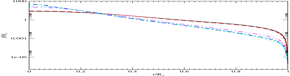
Figure 1: Distributions of the ratio of the density $\rho$ to the mean density $\rho_{*}=3M/(4\pi R_{*}^{3})$ shown as functions of the dimensionless radius $r/R_{*}$. Solid, dashed, dotted, dot dashed, dot dot dashed and dot dashed dashed lines correspond to WASP-43, Ogle-tr-113b, models A and B of WASP-12 and models A and B of WASP-18, respectively.

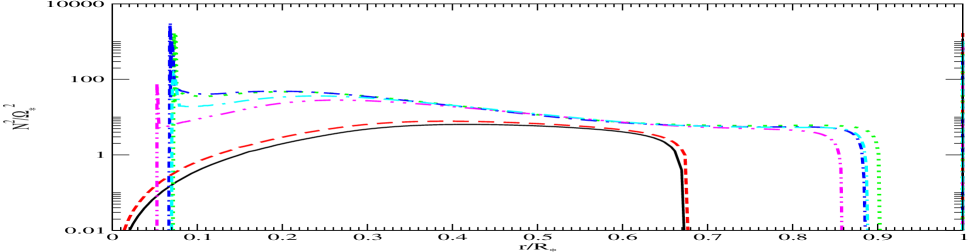
Figure 2: Same as for Fig. 1, but the distributions of the square of the Brunt - V$\ddot{\rm a}$is$\ddot{\rm a}$l$\ddot{\rm a}$ frequency are shown.

We show the dependence of the density and Brunt - V$\ddot{\rm a}$is$\ddot{\rm a}$l$\ddot{\rm a}$ frequency on radius for each of the stellar models in Figs. 1 and 2. One can see that the models of WASP-12 and WASP-18 are more centrally condensed than those of the others. The difference between the models of WASP-12 and WASP-18 and those of WASP-43 and Ogle-tr-113b is even more prominent when the respective distributions of the Brunt - V$\ddot{\rm a}$is$\ddot{\rm a}$l$\ddot{\rm a}$ frequency are compared. The Brunt - V$\ddot{\rm a}$is$\ddot{\rm a}$l$\ddot{\rm a}$ frequency is expressed in units of the inverse of the characteristic stellar dynamical time scale $\Omega_{*}=\sqrt{GM/R_{*}^{3}}$. While the latter models have convective envelopes and radiative cores, and are in general similar to solar models the former models have small convective cores and radiative envelopes. This distinction is a consequence of the difference in stellar masses and is expected for stars on the main sequence. The masses of WASP-43 and Ogle-tr-113b are approximately equal to $0.7M_{\odot}$, while WASP-18 and WASP-12 are significantly more massive, having masses $M\approx 1.2-1.3M_{\odot}$.

4.1.1 Stellar rotation

For Ogle-tr-113, WASP-12 and WASP-18 we use the data on projected rotational velocities listed in Schlaufman (2010) and assume that the inclination angle between rotational axes and the line of sight is close to $\pi/2$. We thus respectively obtain rotational periods, $P_{r}$, approximately equal to 7.79d, 37d and 5.39d for these systems. In case of WASP-43 we use the result quoted in Hellier et. al. (2011) that $P_{r}\approx 15.6d$. Of these the rotation periods of Ogle-tr-113 and WASP-18 are closest to the orbital period, thus indicating that for these two systems is there a possibility that the effect of rotation could weaken tidal interactions appreciably. Accordingly, we consider this effect only for these two systems below.

In addition we remark that there are indications that the orbit of WASP-12 is strongly misaligned with the stellar equatorial plane (Albrecht et al., 2012). This means that additional tidal effects to those we consider can play a role. However, the stellar rotation period is estimated to exceed the orbital period by more than an order of magnitude. Accordingly, as indicated above, it should be reasonable to neglect rotation when considering orbital decay. Nonetheless the misalignement will result in tidal forcing associated with azimuthal mode number, $m=1,$ in addition to that with $m=2$ considered in this paper. This will excite stellar modes leading to dissipation that is expected to cause evolution towards alignment (see eg. Papaloizou & Pringle, 1982). As long as tides remain linear this effect should be decoupled from orbital decay.

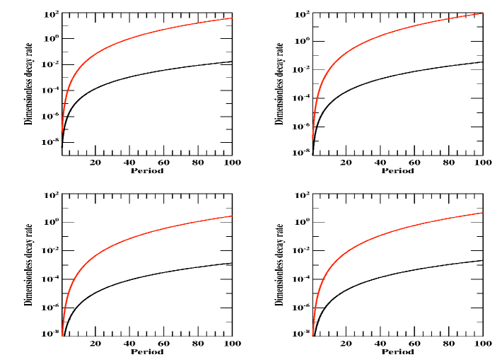
Figure 3: Each of the panels shows the ratio of the decay rate of a normal mode to its angular frequency, $\gamma/\omega$ ( black curve ) and the ratio of the decay rate of a normal mode to the mode angular frequency interval, $\gamma/(d\omega/dn)$ (red curve) for stellar models in the vicinity of the main sequence, as functions of the orbital period $4\pi/\omega$ in days. The upper left panel corresponds to WASP-18, the upper right panel to WASP-12, the lower left panel to WASP-43 and the lower right panel to Ogle-tr-113 respectively.

4.1.2 Properties of normal mode decay rates

Following the procedure outlined in sections 2.2 and 2.3 we evaluated the normal mode decay rates as a function of forcing frequency, $\omega,$ corresponding to the excited mode frequency. This is twice the orbital angular velocity in the case of a circular orbit, which will be assumed for the purpose of estimating whether the MLD limit applies in this section.

The ratio of the decay rate of a normal mode to its angular frequency, $\gamma/\omega,$ and the ratio of the decay rate of a normal mode to the mode angular frequency interval, $\gamma/(d\omega/dn)$ is shown for main sequence models as a function of the putative orbital period $4\pi/\omega$ in Fig. 3. Note that these are considered as continuous functions of $\omega$, even though the normal modes take on discrete values. However, the frequency interval separating consecutive modes is small such that viewing the relevant quantities as continuous functions is reasonable.

The models considered are for WASP-43, Ogle-tr-113, model A for WASP-12 and model A for WASP-18. We remark that models B give very similar results to models A. We see that the models for WASP-43 and Ogle-tr-113 produce similar results as do the models for WASP-12 and WASP-18. The latter pair have values for $\gamma/\omega,$ and $\gamma/(d\omega/dn)$ that are characteristically $30$ larger at a given orbital period than those appropriate to the former pair. For all models and periods less than $100$ days, $\gamma/\omega<\sim 0.03,$ indicating validity of the quasi-adiabatic approximation. However note that this quantity $<\sim 10^{-8}$ at periods of, $\sim 3d,$ characteristic of Hot Jupiters. The quantity $\gamma/(d\omega/dn)$ that we use to indicate whether the MLD regime applies exceeds unity only for periods exceeding about $80$ days in the case of WASP-43 and Ogle-tr-113 and for periods exceeding about $35$ days in the case of WASP-12 and WASP-18. Thus the MLD limit does not apply to any of these systems for the period range appropriate to Hot Jupiters if linear radiative dissipation alone is considered.

4.2 Kepler-91: an example of an evolved star

We now consider Kepler-91 which is an example of a star which has evolved off main sequence to move along the giant branch. The main parameters of the observed star are summarised in table 3 and the physical and orbital parameters of its companion close-in planet, Kepler-91b, are given in table 4 The evolution of the radius of Kepler-91 as a function of time is illustrated in Fig. 4. It will be seen that Kepler-91 is currently evolving with a rapidly increasing radius. Therefore, as indicated above it is important to consider a set of models with different ages, $T_{age}$, and to calculate the overlap integrals and orbital evolution rates corresponding to this set of models.

	$M$	$R_{*}$	[Fe/H]	$T_{\rm eff}$	age
Kepler-91	1.31$\pm$0.1$M_{\odot}$	6.3$\pm$0.16$R_{\odot}$	0.11$\pm$0.07	4550$\pm$75 K	4.86$\pm$2.13Gyr
Model	1.31$M_{\odot}$	6.30$R_{\odot}$	0.10	4735 K	4.26Gyr
HD32518	1.13 $\pm$ 0.18 $M_{\odot}$	10.22 $\pm$ 0.87$R_{\odot}$	-0.15 $\pm$ 0.04	4580 $\pm$ 70 K	5.83 $\pm$2.58 Gyr
Model	1.13$M_{\odot}$	10.20$R_{\odot}$	-0.15	4612 K	6.76Gyr

Table 3: Same as for table 1, but for the stars, Kepler-91 (see e.g. Lillo-Box et al., 2014)

and HD32518 (see Döllinger et al., 2009) .

	$m$	$R_{pl}$	$P_{orb}$	e
Kepler-91b	0.73$\pm$0.13$M_{J}$	1.384$\pm$0.054$R_{J}$	6.2466 d	0.066$\pm$0.013
HD32518b	$3.04\pm$0.68$M_{J}$	N/A	157.54 d	0.01$\pm$0.03

Table 4: Same as for table 2 but for the exoplanets, Kepler-91b
(see e.g. Lillo-Box et al., 2014; Barclay et al., 2014) and
HD32518b (see Döllinger et al., 2009).

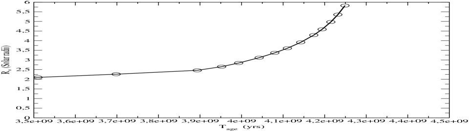
Figure 4: The evolution of the radius of Kepler-91 (shown in units of the Solar radius) as a function of time. Circles show the positions of particular stellar models used in our computations.

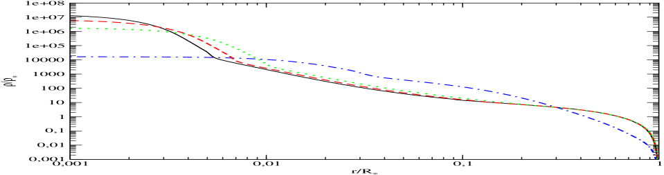
Figure 5: The dependence of density of the model of Kepler-91 specified in table 3 expressed in units of the mean density $\rho_{*}$ on dimensional radius $r/R_{*}$. See the text for a description of particular curves.

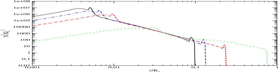
Figure 6: Same as for Fig. 5, but for the square of the Brunt - V$\ddot{\rm a}$is$\ddot{\rm a}$l$\ddot{\rm a}$ frequency expressed in units of $\omega_{*}^{2}=GM/R_{*}^{3}$.

We have checked that tidal evolution is essentially insignificant for $T_{age}<3.5Gyr$. Accordingly we consider 14 stellar models with ages in the range $3.51Gyr<T_{age}<4.26Gyr$, with the time interval between them decreasing at later times to account for more rapid evolution of the star (see Fig. 4). In Figs. 5 and 6 we show, respectively, the density and Brunt - V$\ddot{\rm a}$is$\ddot{\rm a}$l$\ddot{\rm a}$ frequency as a function of radius. Solid, dashed, dotted and dot dashed curves correspond to $T_{age}=4.26$, $4.21$, $4.11$ and $3.7Gyr$, respectively. One can see that at the latest time the stellar structure assumes a typical red giant form with a highly centrally condensed core and an extended convective envelope.

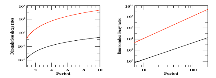
Figure 7: The left panel shows $\gamma/\omega$ ( black curve )and $\gamma/(d\omega/dn)$ (red curve) as functions of the orbital period in days (see the caption to Fig. 3) for the model of Kepler-91 listed in table 3. The corresponding plots for the model of HD32518 also listed in table 3 are shown in the right panel.

4.2.1 Properties of normal mode decay rates

Following the procedure outlined in sections 2.2 and 2.3 we evaluated the normal mode decay rates as a function of forcing frequency, $\omega,$ for the model of Kepler-91 listed in table 3. For reference purposes we also did this for the model of HD32518 also listed in table 3. This is also on the giant branch. The ratio of the decay rate of a normal mode to its angular frequency, $\gamma/\omega,$ and the ratio of the decay rate of a normal mode to the mode angular frequency interval, $\gamma/(d\omega/dn)$ is shown as a function of $\omega$ for these models in Fig.7.

For Kepler-91, $\gamma/\omega<\sim 0.1,$ for periods less than $10$ days justifying validity of the quasi-adiabatic approximation. Note that this quantity $\sim 0.03$ at a period of $6.25$ days corresponding to Kepler-91b. The quantity $\gamma/(d\omega/dn)>1$ for periods exceeding $1.5$ days, indicating that the MLD regime applies for orbital periods characteristic of Hot Jupiters. In the case of HD32518, $\gamma/\omega~{}<~{}\sim~{}1,$ for periods $<8$ days with $\gamma/(d\omega/dn)>1$ for periods of a few days showing again that the MLD regime holds. Note that for an orbital period of $157.5$ days corresponding to HD32518b, $\gamma/\omega\sim 10^{4}$ demonstrating a dramatic failure of the quasi-adiabatic approximation. In this case $g$ modes are not excited indicating that an equilibrium tide approach should be followed.

5 Tidal evolution

5.1 Results for Main sequence stars

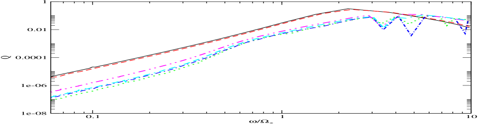
Figure 8: Overlap integrals as functions of mode eigenfrequency for the main sequence stellar models.for which orbital evolution was considered. Solid, dashed, dotted, dot dashed, dot dot dashed and dot dashed dashed curves correspond to WASP-43, Ogle-tr-113, WASP-12, models A and B, and WASP-18, models A and B, respectively.

In order to calculate the orbital evolution by solving (1) - (4) it is necessary to evaluate the overlap integrals for the stellar model under consideration (Chernov, 2017). We show overlap integrals, $Q_{k}$, obtained for our models of main sequence stars in Fig. 8. For all models $Q_{k}$ is found to sharply decrease as $\omega_{j=j(k)}$ decreases.

In case of WASP-43 and Ogle-tr-113 the shape of the curves is very similar to what is obtained from a Solar model, while in the case of WASP-12 and WASP-18 the results are closer to those obtained for more massive stars (see e.g. Chernov et al., 2013, (ChIP)). At a given frequency, $Q_{k}$ is markedly smaller in the latter case as compared to the former case. This is attributed to a smaller relative size of the convective envelope in the models of WASP-12 (see ChIP).

	$\omega=2\Omega_{orb}$	$|d\omega_{j}/dj||_{j(k)}$
WASP-43	1.7879e-4	1.1086e-5
WASP-12A	1.3326e-4	3.7050e-06
WASP-12B	1.3326e-4	4.0569e-06
Ogle-tr-113	1.0153e-4	3.4381e-6

Table 5: Values of the forcing frequency and the frequency separation between successive normal modes in its vicinity for some non-rotating stellar models in seconds^-1.

We also give, for a reference, the values of the forcing frequency $\omega=k\Omega_{orb}$ and the frequency difference between two neighbouring modes for the mode which is closest to resonance, $|d\omega_{j}/dj|_{j(k)}$, for the stellar models considered in detail in table 5. We take $k=2,$ which is the case of interest for our calculations and neglect the effect of rotation. We note that the decay rate of the mode nearest to resonance is given by $\gamma=\kappa|d\omega_{j}/dj|_{j(k)}$. From table 5 we see that, $|d\omega_{j}/dj|_{j(k)}\ll 2\Omega_{orb}$, is small corresponding to a dense spectrum of modes, thus justifying the use of formalism developed in IPCh.

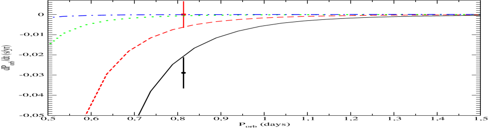
Figure 9: Results related to our model of WASP-43 are shown. Different curves represent the time derivative of orbital period, $\dot{P}_{orb}$, in units of $s/yr$ as functions of orbital period in days, for different values of the quantity $\kappa$ parametrising mode dissipation rate. See the text for a description of particular curves. The black circle and red square show the positions of two proposed values of $\dot{P}_{orb}$ inferred from analysis of observational data by Jiang et al. (2016) and Hoyer et al. (2016b), respectively.

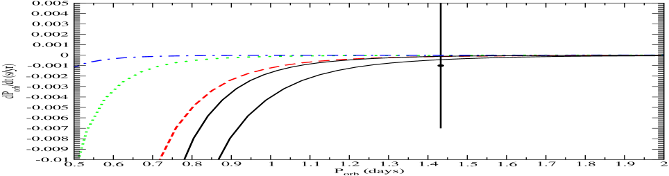
Figure 10: Same as Fig. 9, but for the star Ogle-tr-113. Note that in this case there are two solid curves corresponding to the MLD regime, the curve taking on smaller (larger) values at a given $P_{orb}$ corresponds to the non-rotating (rotating) star. The value of $\dot{P}_{orb}$ obtained from observations and its error bar are taken from Hoyer et.al. (2016a).

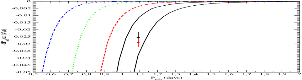
Figure 11: Same as Fig. 9, but for the star WASP-12. The solid curve with smaller (larger), $|\dot{P}_{orb}|$, corresponds to model A (B). The other curves correspond to model A. The indicated positions of the value of $\dot{P}_{orb}$ obtained from observations and their error bars are taken from Maciejewski et al. (2016) and Patra et al. (2017), with smaller and larger absolute values of $\dot{P}_{orb}$ corresponding to the former and latter references, respectively.

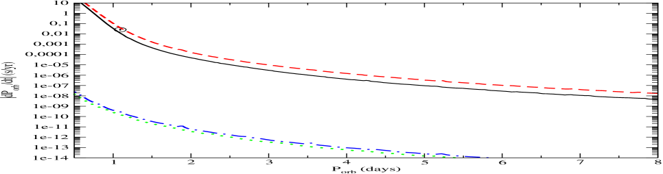
Figure 12: $|\dot{P}_{orb}|$ as a function of orbital period. Solid and dashed curves, obtained with the use of our formalism, respectively correspond to models A and B for WASP-12. The dotted and dot dashed curves are calculated according to the Zahn prescription, applied to models A and B, respectively. All curves have been calculated in the assumption that the MLD regime applies.

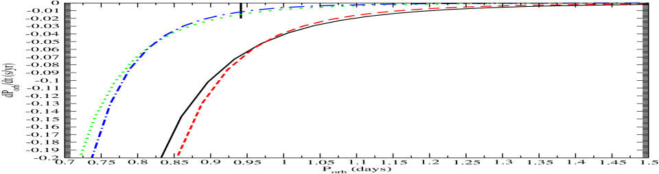
Figure 13: $\dot{P}_{orb}$ as a function of orbital period calculated for the system WASP-18. The vertical solid line indicates the published observational limits on the orbital evolution of the system. All theoretical curves are calculated assuming the MLD regime. Solid and dashed lines show the theoretical results for models A and B and assuming a non-rotating star respectively The dotted and dashed lines are respectively for models A and B but with the star assumed to have $P_{r}=5.39d.$

We use these overlap integrals in equations (1)-(4) to enable the orbital evolution to be calculated together with the time derivative of orbital period, $\dot{P}_{orb}.$ Results of the calculations of, $\dot{P}_{orb},$ together with data inferred from observations, are shown in Figs. 9, 10 and 11, for the models of WASP-43b, Ogle-tr-113b and WASP-12b, respectively. Solid, dashed, dotted and dot dashed curves respectively correspond to a formally infinite value of $\kappa$ making $D=1,$ implying the MLD regime, $\kappa=0.1$, $0.01$ and $0.001.$ We have checked that the result corresponding to $\kappa=1$ gives a curve almost indistinguishable from the solid one. In addition, for values of $\kappa<0.001,$ $\dot{P}_{orb}\propto\kappa,$ as follows from equation (8).

Two different values of $\dot{P}_{orb}$ obtained from analysis of observational data are indicated in Fig. 9. A relatively large value of $|\dot{P}_{orb}|\sim 0.03s/yr$ was reported by Jiang et al. (2016), whereas Hoyer et al. (2016b) claim that $|\dot{P}_{orb}|$ is significantly smaller and consistent with zero. As seen from Fig. 9 the larger value of $|\dot{P}_{orb}|$ can be easily explained by as resulting from tidal evolution in the MLD regime. On the other hand if the result of Hoyer et al. (2016b) holds, the action of tides in this systems is very much weaker than that predicted within the framework of that regime.

In the limit of weak dissipation, when the system is mid way between resonances, the evolution rates, including, $|\dot{P}_{orb}|,$ have to be multiplied by a factor $\pi\kappa=\pi\gamma/(|d\omega_{j}/dj|_{j=j(k)})$ (see equation (9) and discussion above). For WASP-43 we find that this quantity is $\sim 4\times 10^{-8}$ resulting in an extremely small $|\dot{P}_{orb}|\sim 10^{-9}s/yr.$ Thus, the observational result of Hoyer et al. (2016b) is consistent with tides being in the linear regime with radiative damping operating in the weakly dissipative limit.

In the case of Ogle-tr-113b, which is a relatively fast rotator, we show $\dot{P}_{orb}$ calculated in the MLD regime for a non-rotating star, and for a star with rotational period $P_{r}=7.79d$ in Fig. 10, with solid curves taking on respectively smaller and larger values at a given $P_{orb}.$ Note that in the latter case we assume that the resonant frequency is expressed in terms of the orbital frequency and the angular frequency of rotation, $\Omega_{r}=2\pi/P_{r}$, through $\omega=2(\Omega-\Omega_{r})$.

In the case of Ogle-tr-113b, Fig. 10 shows that the value of $|\dot{P}_{orb}|,$ obtained from observations is consistent with the system operating in the MLD regime, with the mean value being very close to the theoretical curve for the non-rotating case. However, the reported observational errors are so large that even positive values of $\dot{P}_{orb}$ are not excluded. Accordingly, no definite conclusion about the regime in which tides operate can be made in this case.

The results presented in Fig. 11 for WASP-12 indicate that the MLD regime is fully compatible with the available data. Model A gives a slightly smaller value of $|\dot{P}_{obs}|$ than that is obtained from observation, while model B gives a slightly larger value. It is evident that one could obtain a perfect agreement using a model of WASP-12 with parameters intermediate to those have been employed in models A and B.

Since WASP-12 is a star possessing a convective core, albeit a small one, as a matter of interest we can apply the theory of Zahn (1970, 1977) to this star and compare results. This comparison is shown in Fig. 12, where we plot absolute values of $\dot{P}_{orb}$ calculated in the framework of our formalism, under the assumption of the MLD regime, as solid and dashed lines and in the Zahn theory as dotted and dot dashed lines, for models A and B, respectively. One can see that our approach gives very much larger tidal evolution rates, being $\sim 10^{9}$ times larger than given by the the Zahn theory. This result is, however, expected since this discrepancy arises because the Zahn theory is based on the modes being excited at the outer boundary of convective core, which has small radius (see Fig. 2 ), whereas in our case the important region is near the inner boundary of the convective envelope, see also Goodman& Dickson (1998).

Finally, let us discuss the system WASP-18. For this system we present theoretical dependencies of $\dot{P}_{obs}$ on $P_{obs}$ in Fig. 13. All curves are obtained assuming that the MLD regime operates. We see that the results obtained for the non-rotating star are clearly incompatible with the observational limits. However, when the effect of stellar rotation is taken into account both models considered are within the limits. Interestingly, these models predict $|\dot{P}_{orb}|\approx 0.01-0.015s/yr$, which is just slightly smaller that the published upper bound $|\dot{P}_{orb}|<0.02s/yr$. Thus, observations should allow us to either confirm or discard the possibility that tidal interactions occur in the MLD regime in this system in the near future.

In summary, the limited observations available suggest that main sequence stars orbited by close giant companions could sometimes be in the MLD regime and sometimes not. The latter case is what would be expected from the linear theory of tides for which radiative damping operates. In the former case non-linearity needs to be invoked in order to provide adequate dissipation (see eg. Barker & Ogilvie, 2011). It is clear that more observations are needed in order to make a robust conclusion about whether and how often tidal evolution operates in the MLD regime in systems containing main sequence stars and close-in Hot Jupiters.

5.2 Kepler-91b

We now consider the tidal evolution of Kepler-91b. As can be seen from Figs. 5 and 6 the star Kepler-91 is a red giant with an extended convective envelope. This means that in addition to $g$ modes being excited by tides there could be other significant factors influencing orbital evolution including effects due to quasi-static tides, as well as effects associated with a powerful stellar wind, namely stellar mass loss, mass accretion by the planet and hydrodynamic drag exerted on the planet by the wind. To take account of these, we write the equations governing orbital evolution in the form

$${\dot{a}\over a}=-{2\over T_{a}}-{2\over T_{a,QSt}}+{\left({\dot{a}\over a}\right)}_{W}\quad{\rm and}\quad{\dot{e}\over e}=-{1\over T_{e}}-{1\over T_{e,QSt}}+{\left({\dot{e}\over e}\right)}_{W},$$ (27)

where $T_{a}$ and $T_{e}$ are given by equations (2) - (4) and the quantities subscripted with, $QSt,$ and, $W,$ represent rates of change of the orbital parameters due to the action of quasi-static tides and the stellar wind, respectively. We note that as discussed in Section 4.2.1, the MLD regime is expected to apply for the current model of Kepler-91 and the orbital periods we have considered. Thus standing waves and resonant modes cannot be set up (see Section 2.1). This means that resonance locking is not expected to be occurring at the present evolutionary stage. We go on to discuss quasi-static tides and the stellar wind in turn.

5.2.1 Quasi-static tides

We follow Zahn (1977) and assume that tidal dissipation takes place as a result of turbulent viscosity acting on the quasi-static equilibrium tide in the convective envelope. We treat quasi-static tides in the simplest possible approximation using the results of Zahn (1989), namely, we use equation (17) of that paper for the evolution of semi-major axis and equation (18) of that paper for the evolution of eccentricity. We set the angular velocity of stellar rotation and the orbital eccentricity to zero in the right hand side of these equations. The characteristic time scales of orbital evolution due to quasi-static tides, $T_{a,QSt}$ and $T_{e,QSt}$, are shown in Appendix as euqations (35) and (36), respectively. They depend on parameters $\lambda_{l}$ defined in equations (37) and (38), for $l=1,2,3,$, where $l$ are numbers of Fourier harmonics in the decompostion of the perturbing potential in Fourier series in time. They in turn depend on the quantities $\eta_{l}=2lt_{f}/P_{orb}.$ Here $t_{f}$ is the characteristic time of turnover of convective eddies defined as

$$t_{f}=\left({M_{*}R_{*}^{2}}\over{L}\right)^{1/3}.$$ (28)

The weakening of turbulent viscosity in the regime of $\eta_{l}\gg 1$ as noted by eg. Goldreich & Nicholson (1989), results in reduction of $\lambda_{l}$ with increasing $\eta_{l}$. The form of the dependence of $\lambda_{l}$ on $\eta_{l}$ that should be used is unknown. In the past a power-law dependence with either $\lambda_{l}\propto\eta_{l}^{-2}$ (eg. Goldreich & Nicholson, 1989) or $\lambda_{l}\propto\eta_{l}^{-1}$ ( e.g. Zahn, 1989) has been assumed. However, the actual situation may be more complex with the effective viscosity even being negative in some cases (see Ogilvie & Lesur, 2012). Here, for simplicity, we shall treat this dependency in the simplest possible way. Namely, when $\eta_{l}<1$ we use equation (13) of Zahn (1989) when calculating $\lambda_{l}$. Then these quantities are found not depend on $\eta_{l}$ and $l$ so we may write $\lambda_{l}\equiv\lambda.$ When $\eta_{l}>1$ we adopt $\lambda_{l}=\lambda/\eta_{l}.$

In order to calculate $\lambda$ we use parameters such as radius of the base of convective envelope, etc. for a grid of models with different ages, that is used for our calculation of the effect of dynamic tides on the orbit. We find $T_{a,QSt}$ and $T_{e,QSt}$ for these models and use linear interpolation to obtain them for intermediate ages of the star. In following the procedure outlined above, we stress the considerable uncertainty in estimating the effects of turbulence acting on quasi-static tides and that the effective turbulent viscosity and consequent effects on orbital evolution may be significantly overestimated.

5.2.2 Stellar wind

In order to evaluate the rate of mass loss from stellar wind, $\dot{M}_{W}$, we use the Reimers law (Reimers, 1975)

$$\dot{M}_{W}=4\cdot 10^{-13}\eta_{R}\left({L\over L_{\odot}}\right)\left({M\over M_{\odot}}\right)\left({R_{\odot}\over R_{*}}\right)M_{\odot}/yr^{-1},$$ (29)

where $L$ is the stellar luminosity. From the conservation of angular momentum it follows that the semi-major axis will evolve as a result of the mass loss according to

$$\left({\dot{a}\over a}\right)_{W}={\dot{M}_{W}\over M}.$$ (30)

Thus it will take on larger values as a result of a positive rate of mass loss.

One can see that the change of the gravitational field of the star due to mass loss does not lead to an appreciable change of orbital eccentricity since both the eccentricity and the angular momentum are adiabatic invariants when the orbit changes on account of the changing mass of the central star. Accordingly, we set $\dot{e}_{W}=0$.

5.2.3 Hydrodynamic drag

Let us estimate the effect of hydrodynamical drag exerted on the planet. We first calculate the ratio of Bondi-Hoyle radius $R_{BH}=2Gm/(v_{k}^{2}+c^{2}_{s})$, where $v_{k}$ is Keplerian velocity taken to be $v_{k}=\sqrt{GM/a}$ for a near circular orbit, and $c_{s}$ the sound speed of the wind, to the planet radius $R_{pl}.$ This is easily done with help of tables 3 and 4 together with the assumption that $c_{s}\sim 30km/s\ll v_{k},$ with the result that $R_{BH}/R_{pl}\sim 0.16$.

This means that gas trajectories are not significantly deflected by the planet’s gravitational field before meeting the planet. Thus, to make a rough estimate of the rate of energy exchange with the planetary orbit per unit of time, $\dot{E}_{HD}$, we can simply calculate the rate of energy flow due to gas elements moving with Keplerian velocity through a target with cross-section equal to $\pi R_{pl}^{2}$. This gives

$$\dot{E}_{HD}\sim-{\pi\over 2}\rho R_{pl}^{2}\left({GM\over a}\right)^{3/2}=-{1\over 8}\left({R_{pl}\over a}\right)^{2}\left({GM\over a}\right)^{3/2}{1\over v_{W}}\dot{M}_{W},$$ (31)

where the negative sign occurs because hydrodynamic drag decreases the orbital energy, $\rho$ is the wind density and we have used the law of mass conservation for the wind in the form $\rho~{}=~{}\dot{M}_{W}/(4\pi a^{2}v_{W}).$ The rate of change of orbital semi-major axis is then found from setting

$$\dot{E}_{HD}=\frac{GmM}{2a^{2}}\dot{a}_{HD},$$ (32)

where $\dot{a}_{HD}$ is the rate of change of semi-major axis due to hydrodynamic drag. Combining (32) (31) and (32) we obtain

$$\left({\dot{a}\over a}\right)_{HD}\sim-{1\over 4}\left({R_{pl}\over a}\right)^{2}{v_{K}\over v_{W}}{\dot{M}_{W}\over m}.$$ (33)

It is convenient to express $({\dot{a}/a})_{HD}$ in terms of $({\dot{a}/a})_{W}$ by writing $({\dot{a}/a})_{HD}=-f({\dot{a}/a})_{W}$, where the explicit form of the parameter $f$ follows from (30) and (33) as

$$f={1\over 4}\left({R_{pl}\over a}\right)^{2}{v_{K}\over v_{W}}{M\over m}\approx 0.1\left({30km/s\over v_{W}}\right),$$ (34)

where we have used the parameters given in table 4 in order to obtain the last equality.

Equation (34) tells us that effects due to hydrodynamic drag are expected to be smaller than those associated with the change of mass of the star unless the wind velocity is unrealistically small $v_{W}<3km/s$. Therefore, we shall neglect hydrodynamic drag in our analysis of the orbital evolution of Kepler-91b.

5.2.4 Orbital evolution

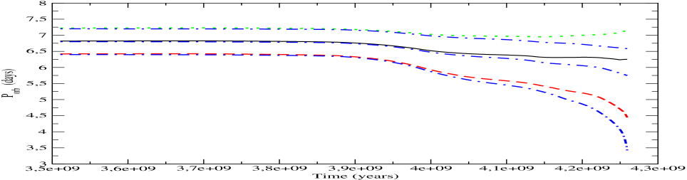
Figure 14: The evolution of orbital period obtained using our model of the tidal interaction of Kepler-91b. Solid, dashed and dotted curves correspond to different initial orbital periods taken when the age of the star was $T_{in}=3.5Gyr$ and evolution of the system was derived from equation (27). The dot dashed curves are for the same initial periods, but with the influence of effects associated with the stellar wind and quasi-static tides being neglected.

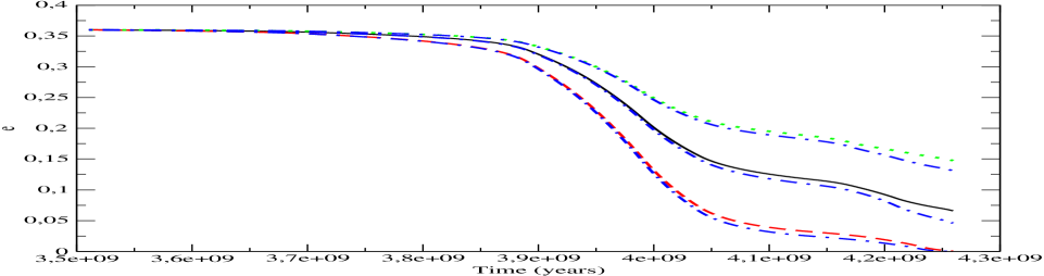
Figure 15: Same as Fig. 14, but for the evolution of eccentricity with time. The initial eccentricity $e_{in}$ was taken to be equal to $0.36$ in all cases.

As already stated above we calculated $T_{a}$ and $T_{e}$ for the set of models of Kepler-91 with different ages and linearly interpolated them to be able to find these time scales at an arbitrary intermediate age. Then, we integrated equation (27) numerically, taking into account, in addition to the excitation of $g$ modes in the MLD regime, the effect of quasi-static tides in the approximation specified above, and the effect of changing gravitational field of the star due to mass loss. The results for the evolution of orbital period and eccentricity are respectively shown in Fig. 14 and Fig.15.

Our evolutionary tracks depend on the values of the orbital period and eccentricity adopted at the initial time taken to be when the age of the star was $T_{in}=3.5Gyr.$ These were chosen in such a way that the solid curves in Figs. 14 and 15 reproduce the observed values, $P_{orb}(T_{fin})\approx 6.25d$ and $e(T_{fin})\approx 0.066$ at final time when the age of the star was $T_{fin}=4.26Gyr$ as currently estimated (see table 3). This requires $P_{orb}(T_{in})\approx 6.8d$ and $e(T_{in})\approx 0.36$. Thus tidal evolution can diminish a rather large value of initial eccentricity to the small observed value, while the value of orbital period changes by less than 10 per cent. Dashed and dotted curves show the results corresponding to slightly smaller and slightly larger initial orbital periods, $P_{orb}(T_{in})\approx 6.4d$ and $P_{orb}(T_{in})\approx 7.2d$, respectively. One can see from Figs. 14 and 15 that the evolution looks rather different for these cases as compared to the case fitting the data. While the case with smaller initial period shows a violent tidal evolution at late times leading to a strong decrease of orbital period, the case with larger initial period is such that the period increases at late times due to the effect of mass loss from the star. This feature could lead to an understanding of the present day orbital parameters of Kepler-91b, since tidal and mass loss effects on the evolution of the semi-major axis can be nearly balanced, while at the same time, tidal effects lead to significant decrease of eccentricity. Note that the results plotted in Figs. 14 and 15 show that quasi-static tides considered in our approximation, which we argued are likely to be overestimated, do not significantly influence the evolution of the system.

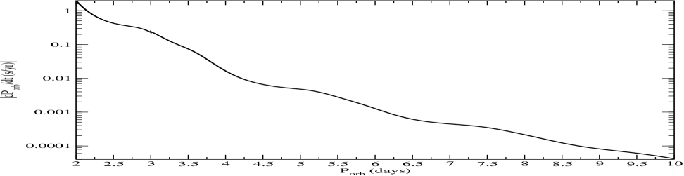
Figure 16: $|\dot{P}_{orb}|$ as a function of orbital period for a star with parameters of the present day model of Kepler-91 and a planet with the mass of Kepler-91b.

Finally, for reference and comparison with the main sequence models, we show the dependence of the absolute value of $\dot{P}_{orb}$ on the orbital period for a system containing a star with parameters appropriate to the present day state of Kepler-91 and a planet with the mass of Kepler-91b. Only dynamic tides in the MLD regime are taken into account in this calculation. One can see that at orbital periods of ${}^{\prime}\sim 6d$ corresponding to Kepler-91b, $|\dot{P}_{orb}|$ is rather small, being of the order of $0.001s/yr$. Note too that the effect of mass loss would reduce it still further.

6 Discussion and Conclusions

In this Paper we have applied our general formalism for determining effects due to dynamical tides developed in Ivanov et al. (2013) (IPCh) to calculate the expected orbital evolution in observed systems containing a Hot Jupiter. Our formalism is based on the normal mode approach to the problem, it contains within it the well known Zahn theory of dynamical tides. Contrary to the Zahn theory, which applies only in the asymptotic limit of small tidal forcing frequencies and only for hot stars with convective cores and radiative envelopes (see Zahn, 1970, 1977), our formalism allows one to consider more general and realistic stellar models together with forcing frequencies that are not asymptotically small. We pay special attention to the question of whether or not the assumption that the propagation time of wave trains excited by tides through propagation zones, is longer than their dissipation time, corresponding to the regime of moderately large dissipation (MLD), is supported by the analysis of present day observations. We note in passing that the Zahn theory is applicable in this regime also.

We consider several main sequence (MS) stars with Hot Jupiter companions, for which either the rate of change of orbital period, $\dot{P}_{orb}$, or an upper limit for it have been reported, as well as the evolved star Kepler-91, which has a Jupiter mass companion, Kepler-91b, on a close in orbit. We demonstrate that although the linear mechanism of radiative damping of tidally excited modes is not effective enough to justify the assumption of the MLD regime for the systems containing a main sequence star, it results in the Kepler-91 system evolving in the MLD regime. We recall that in cases for which the MLD regime does not operate, relatively weak dissipation is implied unless there is a resonance with a normal mode.

6.1 Systems with stars on the main sequence

The systems containing MS stars and Hot Jupiters we considered in Section 5.1 were WASP-43, Ogle-tr-113, WASP-12 and WASP-18. The former two contain Sun-like stars with radiative interiors and convective envelopes, while the latter two are relatively more massive and have the complimentary structure with convective cores and envelopes which are for the most part radiative with there being a relatively small convective region near the surface. We remark that on account of their low mass and the mismatch between the convective turn over time and the inverse tidal forcing frequency, tidal dissipation in these envelopes is expected to be ineffective (see eg. Barker & Ogilvie, 2011). In addition, the stars, Ogle-tr-113 and WASP-18 appear to be rotating sufficiently rapidly that the effect of rotation should to be taken into account when calculating $\dot{P}_{orb}$. Note that this weakens the tidal interaction when the angular momentum vectors associated with stellar rotation and the orbital motion are aligned as has been assumed in this paper.

Values of $\dot{P}_{obs}$ have been obtained for WASP-43 by Jiang et al. (2016) and Hoyer et al. (2016b). Although the former authors give an absolute value of $\dot{P}_{orb}$, which is consistent the assumption of MLD regime, the value given by the latter authors is too small to be consistent with it. WASP-43 appears to be a slow rotator, and, therefore, the inconsistency of this assumption with the analysis of Hoyer et al. (2016b) cannot be alleviated by taking rotation into account. On the other hand it is consistent with being in a weak dissipation regime and the tidal forcing frequency being mid way between neighbouring normal mode frequencies.

In case of Ogle-tr-113, models with tides operating in the MLD regime with and without rotation are consistent with the present observations. However, error bars are so large that even positive values of $\dot{P}_{obs}$ are not necessarily excluded.

WASP-12 appears to show the best consistency with the assumption of being in the MLD regime. Errors bars are small enough in this case to accommodate results provided by both of our models for this star. Note, however, that Patra et al. (2017) also consider another scenario for the observed changes in occulation times base on apsidal precession giving it, however, less probability that the one based on the orbital decay due to tides. It is of interest to note that a direct application of the Zahn theory to this system gives values of $\dot{P}_{obs}$ that are orders of magnitude smaller ( see Fig. 12) .

Finally, in the case of WASP-18 only an upper limit given by $|\dot{P}_{obs}|<0.02s/yr$ is inferred from the lower limit on the modified tidal quality factor, $Q^{{}^{\prime}}>10^{6},$ recently published by Wilkins et. al. (2017). Although this limit certainly excludes MLD tides operating in non-rotating stars, MLD tides in the star rotating with rotational period $\sim 5.4d$ are in marginal agreement with the published bound on $|\dot{P}_{obs}|$ giving $|\dot{P}_{obs}|\approx 0.01-0.015s/yr,$ depending on the stellar model. Thus in case of this system, a relatively minor reduction in the magnitude of the observational error, could either confirm or exclude the MLD regime.

As we have discussed in Section 4.1.2, the assumption of the MLD regime, cannot be justified assuming the theory of linear damping of tidally excited modes due to radiative diffusion applies to the considered MS stars. Thus, some mechanism of non-linear mode damping must be invoked to account for the possibility of this regime applying for these objects. Since both WASP-43 and Ogle-tr-113 are Sun-like we can check whether or not they satisfy the criterion for wave breaking in their radiative cores given by Barker & Ogilvie (2011) . We found out that this criterion is not satisfied, with characteristic mode amplitudes near the centre being several orders of magnitude smaller than needed. This is explained by relatively young ages of WASP-43 and Ogle-tr-113. As discussed in Barker & Ogilvie (2011) the wave amplitude near the centre of a MS star is proportional to a positive power of the gradient of the Brunt - V$\ddot{\rm a}$is$\ddot{\rm a}$l$\ddot{\rm a}$ frequency, and this is relatively small for young MS stars. A possible non-linear mechanism that could work in the objects with the considered parameters is mode decay through non-linear interactions that produce a large number of ’daughter’ modes. This was recently discussed by Essick $\&$ Weinberg (2016), who indeed found that it can operate in systems with Hot Jupiters with periods of the order of one day.

In summarising our results for MS stars, we would like to stress that the possibility of the MLD regime operating generically in systems containing Hot Jupiters with periods of the order of one day, has not been definitively established at the present time. When theory and observation are compared, it seems that all except WASP-43 are consistent with being in the MLD regime. However, observational error bars are large so this may not in fact be the case. However in the case of WASP-18, observational bounds on $|\dot{P}_{orb}|$ are very close to theoretically predicted values, so that a modest improvement in the former could provide important clarification on this issue.

6.2 Evolved stars

We considered the case of an evolved star with a close in companion of approximately one Jupiter mass, Kepler-91, in Section 4. For this star we have shown in Section 4.2.1, the existence of linear radiative damping implies that the MLD regime holds. This is because of the dense normal mode spectra found for the models of this star, in the frequency ranges of interest leading to a resonant mode of very high order. Accordingly, dynamical tides associated with $g$ modes of very high order are expected to play a role in the orbital evolution of this system.

We found that the time scale for orbital evolution induced by these tides becomes comparable to the time scale for evolution of the star during the later stages. Therefore, stellar evolution must be fully incorporated in the calculations of the evolution of the orbit which will be significant over the lifetime of the star. We found that quasi-static tides appear to give only a minor contribution, at least within the framework of the simple model adopted. This assumed that the effective turbulent viscosity is reduced by the ratio of tidal forcing period to the characteristic turn over time of convective eddies, when this ratio is less than unity. Note that it has been argued that there should be a quadratic reduction in the efficiency of turbulent viscosity in this regime ((eg. Villaver $\&$ Livio, 2009; Goldreich & Nicholson, 1989) (see Section 5.2.1). In that case orbital evolution due to quasi-static tides would be completely negligible for this system. The effect of stellar wind could have been significant for a planet, with present day orbital period slightly larger than that of Kepler-91b, through the effect of mass loss from the system. On the other hand, the effects of hydrodynamic drag exerted on the planet by the wind and gas accretion onto the planet appear to play only a minor role. Note, however, that these effects have been considered having adopted a procedure which may have been oversimplified (see Section 5.2.2). This deserves further investigation as well as a possibly influence of mass loss from the planet due to e.g. its heating by the star.

We find the following orbital evolution is likely to have taken place during the lifetime of Kepler-91b (see Section 5.2.4). It starts to become significant when the star is approximately 3.5 Gyr old with the orbital period $P_{orb}\sim 6.8d$ being only slightly larger than the current value $P_{orb}\sim 6.2d,$ and the eccentricity being rather large $\sim 0.35$. Since the time scale for the evolution of the eccentricity is shorter than that for the evolution of the semi-major axis, the eccentricity relaxes to its present day small value $\sim 0.066$, while the orbital period changes only by a small amount.

We remark that this circularisation occurs independently of effects due to tides raised on the planet which are also expected to lead to circularisation. However, in this context we note that the current orbital period of Kepler-91b is large enough that such tides may not have operated significantly during the life time of the star (see eg. Ivanov & Papaloizou, 2007, 2010). Note that for slightly larger and slightly smaller initial orbital periods the evolution would be qualitatively different. In the former case the orbital period actually increases during the late stages of stellar evolution due to the effect of mass loss from the system. In the latter case dynamical tides are very efficient and the orbit rapidly shrinks during the later evolutionary stages. Thus, the orbital parameters of the present day Kepler-91b are rather special, since within the framework of our model, only for such parameters do we expect efficient orbital circularisation, while strong prior evolution of the semi-major axis is not expected.

Appendix A Time scales of tidal evolution due to quasi-static tides

Here we show, for completeness, the time scale for the evolution of the semimajor axis, $T_{a,QS}$, and the eccentricity, $T_{e,QS}$, due to quasi-static tides, following the paper of Zahn (1989). They have the form

$$T_{a,QS}={1\over 6\lambda_{2}}\left({M_{*}\over m}\right){\left({a\over R_{*}}\right)}^{8}t_{f}$$ (35)

and

$$T_{e,QS}={1\over 3}{\left({5\over 8}\lambda_{1}-\lambda_{2}+{49\over 8}\lambda_{3}\right)}^{-1}\left({M_{*}\over m}\right){\left({a\over R_{*}}\right)}^{8}t_{f},$$ (36)

where

$$\lambda_{l}={1\over\max{(1,\eta_{l})}}\lambda$$ (37)

and

$$\lambda=0.8725E^{2/5}\int^{1}_{x_{c}}x^{22/3}(1-x)^{2}dx.$$ (38)

The dimensionless radius is $x=r/R_{*}$, with $x_{c}$ being its vallue corresponding to the inner boundary of the convective envelope. Note that we set the mixing length parameter $\alpha^{{}^{\prime}}$ as defined in Zahn (1989) to be unity in (38). The factor $E$ entering (38) is obtained by matching the density $\rho_{c}$ at the convective envelope boundary to that obtained from a density distribution in the envelope region, which is assumed to correspond to the structure of an $n=1.5$ polytrope, thus

$$E=3{\rho_{c}\over\bar{\rho}}{\left({5\over 2}{x_{c}\over 1-x_{c}}\right)}^{3/2},$$ (39)

where $\bar{\rho}=(3/4\pi)(M_{*}/R_{*}^{3})$ is the mean density. We obtain $\rho_{c}$, $x_{c}$, $R_{*}$ and $\bar{\rho}$ using the set of numerical stellar models described above.

References

- Albrecht et al. (2012) Albrecht et al., 2012, ApJ, 744, 189
- Adams et al. (2010) Adams, E. R. et.al., 2010, ApJ, 721, 1829
- Barclay et al. (2014) Barclay, T. et al., 2014, ApJ, 800, 46
- Barker & Ogilvie (2009) Barker, A. J., Ogilvie, G. I., 2009, MNRAS, 395, 2268
- Barker & Ogilvie (2011) Barker, A. J., Ogilvie, G. I., 2011, MNRAS, 417, 745
- Birkby et. al. (2014) Birkby, J. L. at al, 2014, MNRAS, 440, 1470
- Chernov (2017) Chernov, S. V., 2017, Astronomy Letters, 43, 186
- Chernov et al. (2013) Chernov, S. V., Papaloizou, J. C. B., Ivanov, P. B., 2013, MNRAS, 434, 1079 (ChIP)
- Christensen-Dalsgaard (1998) Christensen-Dalsgaard, J., 1998, Lecture Notes on Stellar Oscillations, 4th Edition, users-phys.au.dk/jcd/oscilnotes/
- Cowling (1941) Cowling, T. G., 1941, MNRAS, 101, 367
- Döllinger et al. (2009) Döllinger, M. P. et al., 2009, AA, 503, 1311
- Essick Weinberg (2016) Essick, R., Weinberg, N. N., 2016, ApJ, 816, 18
- Fuller et al. (2016) Fuller, J., Luan, J., Quataert, E., 2016, MNRAS, 458, 3867
- Goldreich & Nicholson (1989) Golreich, P., Nicholson, P. D., 1989, Icarus, 30, 301
- Goodman& Dickson (1998) Goodman, J, Dickson, E. S., 1998, ApJ, 507, 938
- Hebb et. al. ( 2009) Hebb, L. et.al., 2009, ApJ, 693, 1920
- Hellier et. al. ( 2009) Hellier, C., et al., 2009, Nature, 460, 1098
- Hellier et. al. ( 2011) Hellier, C., et. al., 2011, AA, 535, L7
- Hoyer et.al. ( 2016a) Hoyer, S. et.al., 2016a, MNRAS, 455, 1334
- Hoyer et al. (2016b) Hoyer, S. et.al., 2016b, AJ, 151, 137
- Ivanov & Papaloizou (2007) Ivanov, P. B., Papaloizou, J. C. B., 2007, MNRAS, 376, 68
- Ivanov & Papaloizou (2010) Ivanov, P. B., Papaloizou, J. C. B., 2010, MNRAS, 407, 160
- Ivanov & Papaloizou (2011) Ivanov, P. B., Papaloizou, J. C. B., 2011, Celestial Mechanics and Dynamical Astronomy, 111, 51
- Ivanov et al. (2013) Ivanov, P. B., Papaloizou, J. C. B., Chernov, S. V., 2013, MNRAS, 432, 2339 (IPCh)
- Jiang et al. ( 2016) Jiang, I.-G. et.al., 2016, ApJ, 151, 17
- Lillo-Box et al. (2014) Lillo-Box J. et al., 2014 AA, 562, 109
- Maciejewski et al. (2016) Maciejewski, G. et.al, 2016, AA, 588, L6
- Ogilvie & Lesur (2012) Ogilvie, G.I., Lesur, G., 2012, MNRAS, 422, 1975
- Papaloizou & Pringle (1982) Papaloizou, J. C. B., Pringle, J. E., 1982, MNRAS, 200, 49
- Patra et al. (2017) Patra, K. C. et al., 2017, arxiv:1703.06582v1
- Paxton et al. (2011) Paxton, B.,et al., 2011, ApJS, 192, 3
- Paxton et al. (2013) Paxton, B.,et al., 2013, ApJS, 208, 4
- Paxton et al. (2015) Paxton, B.,et al., 2015, ApJS, 220, 15
- Rasio & Ford (1996) Rasio, F. A., Ford, E. B., 1996, Science, 274, 954
- Reimers (1975) Reimers, D., 1975, Mem. Soc. R. Sci. Liege, 6th Series, 8, 369
- Schlaufman (2010) Schlaufman, K. C., 2010, ApJ, 719, 602
- Unno et al. (1989) Unno, W., Osaki, Y., Ando, H., Shibahashi, H., 1989, Nonradial Oscilations of Stars (2nd edition) University of Tokyo Press, Tokyo
- Terquem et al. (1998) Terquem, C., Papaloizou, J. C. B., Nelson, R. P., Lin, D. N. C., 1998, ApJ, 502, 788
- Thun et al. (2016) Thun, D., Kuiper, R., Schmidt, F., Kley, W., 2016, AA, 589, 10
- Wilkins et. al. (2017) Wilkins, A. N. et. al., 2017, ApJ, 836, L24
- Witte & Savonije (1999) Witte, M. G., Savonije, G. J.,1999, A&A, 350, 129
- Witte & Savonije (2002) Witte, M. G., Savonije, G. J.,2002, A&A, 386, 222
- Villaver Livio (2009) Villaver, E., Livio, M., 2009, ApJ, 705, L81
- Zahn (1970) Zahn, J.-P., 1970, AA, 4, 452
- Zahn (1977) Zahn, J.-P., 1977, AA, 57, 383
- Zahn (1989) Zahn, J.-P., 1989, AA, 220, 112