General linearized theory of quantum fluctuations around arbitrary limit cycles
Abstract
The theory of Gaussian quantum fluctuations around classical steady states in nonlinear quantum-optical systems (also known as standard linearization) is a cornerstone for the analysis of such systems. Its simplicity, together with its accuracy far from critical points or situations where the nonlinearity reaches the strong coupling regime, has turned it into a widespread technique, which is the first method of choice in most works on the subject. However, such a technique finds strong practical and conceptual complications when one tries to apply it to situations in which the classical long-time solution is time dependent, a most prominent example being spontaneous limit-cycle formation. Here we introduce a linearization scheme adapted to such situations, using the driven Van der Pol oscillator as a testbed for the method, which allows us to compare it with full numerical simulations. On a conceptual level, the scheme relies on the connection between the emergence of limit cycles and the spontaneous breaking of the symmetry under temporal translations. On the practical side, the method keeps the simplicity and linear scaling with the size of the problem (number of modes) characteristic of standard linearization, making it applicable to large (many-body) systems.
Introduction. The advent of modern quantum technologies has triggered the discovery of a plethora of optical, atomic, and solid state devices working in the quantum regime Dowling03 (see also the starting paragraph of Benito16 and the references therein). A first-principles approach leads to a description of such devices as open quantum systems evolving according to nonlinear Hamiltonians and incoherent processes like dissipation GardinerZoller ; BreuerPetruccione ; Carmichael1 ; GardinerZollerI . Mathematically, one has to face master equations for the state of the system or quantum Langevin equations for its operators, which are in general impossible to solve exactly.
On the other hand, quantum nonlinearities are very difficult to observe in the laboratory and therefore most experiments are well described by effective linear models. The most widespread method for obtaining such linear models starting from nonlinear ones is the so-called standard linearization Drummond81 ; Lugiato81 , which consists in a Gaussian-state ansatz centered at the solution of the system’s nonlinear equations in the classical limit CNB14 . The method combines incredible simplicity with pretty good accuracy in regions of the phase diagram where the system shows a finite number of well-spaced classical attraction points. However, it relies on two properties of the system’s state in the classical limit: It has to be stationary and stable along all directions of phase space. The first condition precludes its application to regions where the classical solutions are time dependent (such as limit cycles StrogatzBook ; GrimshawBook , ubiquitous to, e.g., lasing, second-harmonic generation, or optomechanical systems). The second condition excludes the possibility of applying it to systems which, being invariant under continuous transformations of some kind, have a classical solution which breaks that invariance via spontaneous symmetry breaking. This is because Goldstone’s theorem implies the existence of a zero eigenvalue of the linear stability matrix, and hence a direction of phase space which is not damped CNBthesis ; CNB08 ; CNB10 ; Perez06 ; Perez07 .
While standard linearization has been generalized to deal with spontaneous symmetry breaking of spatial, polarization, and phase symmetries CNBthesis ; CNB08 ; CNB10 ; Garcia09 ; Garcia10 ; Lane88 ; Perez06 ; Perez07 ; Reid88 ; Reid89 , an extension capable of dealing with limit cycles remains. In the case of spontaneous symmetry breaking the trick consists on using a phase-space representation of the state to keep track of the phase-space variable associated to the system’s invariance, which will carry the largest part of the fluctuations. Then, the theory can be linearized with respect to any other phase-space variable.
In this work we generalize standard linearization to regions where the classical long-time solution is time dependent, in particular describing a periodic orbit in phase space. Our idea relies on the connection between the emergence of such limit cycles, and the spontaneous breaking of a very particular symmetry: arbitrary translations in time.
For convenience, in this work we introduce the method for single-mode problems, using the driven quantum Van der Pol (VdP) oscillator Walter14 ; Weiss17 ; Lorch16 as an example. The simplicity of this model will allow for comparisons with full numerical simulations. The generalization to multi-mode problems is straightforward, and will be explored in the future for more practical and complex problems such as optomechanical cavities deep into the parametric instability regime Lorch14 ; Qian12 . Moreover, the complexity of the method scales only linearly with the number of modes, providing then an efficient route towards the analysis of many-body systems out of equilibrium such as optomechanical arrays Arrays1 ; Arrays2 ; Arrays3 ; Arrays4 ; ArraysWeiss in the self-sustained oscillations regime.
Van der Pol model. The quantum model for a driven VdP oscillator consists of a single bosonic mode with annihilation operator , whose state evolves according to the master equation Walter14 ; Weiss17
| (1) |
where and the bosonic operators satisfy canonical commutation relations and . The Hamiltonian includes a coherent drive at rate detuned by with respect to the natural oscillation frequency of the oscillator (note that we work in a picture rotating at the driving frequency). The model contains two incoherent terms as well, the first one corresponding to pairs of excitations lost irreversibly at rate (nonlinear losses), and the second one to linear pumping. The rate of the latter is used to normalize the rest of rates and frequencies, while its inverse normalizes time, so that , , , and are dimensionless. We show later that with these choices the classical phase diagram of the system is determined uniquely by and , while determines the strength of the quantum fluctuations.
The method is best introduced by mapping the master equation to a set of stochastic equations. This can be done with the help of phase-space quasiprobability distributions GardinerZoller ; GardinerZollerI ; Carmichael1 ; SchleichBook such as standard Wigner, Husimi, or Glauber-Sudharsan representations. Here we choose the positive P representation Drummond80 ; CarmichaelBook2 ; GardinerZoller ; GardinerZollerI because, unlike the previous representations, it always leads to stochastic equations equivalent to the master equation without any approximation. This representation associates two independent stochastic variables that we denote by and with the annihilation and creation operators and , respectively, in such a way that normally-ordered quantum expectation values and stochastic averages are related by , with . Using standard techniques Drummond80 ; CarmichaelBook2 ; GardinerZoller ; GardinerZollerI ; GardinerBook , we show in SupMat that the stochastic amplitudes evolve according to
| (2a) | ||||
| (2b) | ||||
where , , and are independent white Gaussian noises (real the first two, and complex the last one).
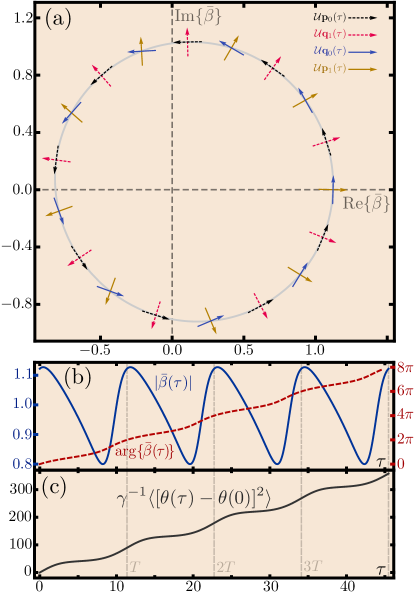
Limit cycles in the classical limit. Coming from a normally ordered representation (where vacuum noise is already taken into account in the ordering), the equations above predict a large-amplitude coherent state for . We talk then about the classical limit. The remaining deterministic equation is a paradigm for synchronization phenomena Weiss17 , and its phase diagram is well known (we provide an overview of it in SupMat ). In general terms, its stationary solutions, corresponding to solutions oscillating at the driving frequency, are stable only provided a strong enough drive is fed; otherwise, the oscillations are not synchronized to the drive, so that for long times the system ends up in a nontrivial stable periodic solution which we call limit cycle or periodic orbit StrogatzBook ; GrimshawBook . In Fig. 1 we show an example of such solution, where it can be appreciated that it describes a closed curve in phase space (a), with an absolute value and a phase that oscillate periodically (b). Note that analytical solutions for these limit cycles exist only in limited cases, and therefore one needs to find them numerically in general.
Linearization around limit cycles. We are now able to introduce the linearization technique for quantum fluctuations around limit cycles. We start by expanding the stochastic amplitudes as
| (3a) | |||
| (3b) | |||
Here, determines at which point of the cycle the solution starts for , and it is precisely the parameter which is not fixed by the classical equations of motion: is a solution of the equations for any choice of . Owed to this symmetry, quantum fluctuations cannot be considered small in arbitrary points and directions of phase space, as nothing prevents them from acting on without resistance. Hence, in order for any linearized theory of quantum fluctuations to work, has to be taken as a variable itself (making it time dependent in the expansion above) and only then the fluctuations and can be taken as small quantities. In addition, can be taken as small quantity as well, since variations of are induced by quantum noise, which is weak in the region of interest. Introducing (3) in (2), to first order in the small variables (including noise) we then get SupMat
| (4) |
where , , , and
| (5) |
is the linear stability matrix. Note that the noise correlations can be written in the compact form , where are the elements of the diffusion matrix
| (6) |
As we will see, the introduction of as an explicit variable will allow us to describe properly spontaneous temporal symmetry breaking and its associated undamped phase-space direction.
Floquet method and eigenvectors. The main difference of Eq. (4) with respect to the linearized Langevin equations found in previous linearization methods is the time periodicity of and . We deal with this by applying Floquet theory CodingtonBook ; GrimshawBook as we explain next.
Let us define the fundamental matrix , which satisfies the initial value problem with , the latter being the identity matrix. From it, we further define the matrix through , and the -periodic matrix . Given the eigensystem of , composed of right and left orthogonal () eigenvectors satisfying and , we introduce the Floquet eigenvectors and . As we show along the next sections, knowledge of these vectors is enough to derive the linearized quantum properties of the system. To this aim, it is also convenient to point out that they satisfy the initial value problems
| (7a) | ||||
| (7b) | ||||
and the orthogonality conditions , as easily proven from their definition.
Let us now comment on the general properties of this eigensystem, which we prove in detail in SupMat . There always exists a null eigenvalue, say , with related (right) Floquet eigenvector . This property is a byproduct of the spontaneous temporal symmetry breaking generated by the limit cycle (Goldstone theorem). In the single-mode case, there is only one other eigenvalue, which is given by , and has associated (left) Floquet eigenvector . This vector is the temporal counterpart of the linear or angular momentum found in previous works which deal with spatial symmetries CNBthesis .
Note that and are, respectively, the tangent and normal vectors of the limit cycle’s trajectory, see Fig. 1(a). We haven’t found explicit expressions of the other Floquet eigenvectors in terms of the , but they can always be found numerically in an efficient fashion, as we do for Fig. 1(a).
Diffusion of the temporal pattern. As a first physical consequence of the properties above, we now show that is diffusing due to quantum noise, and hence quantum fluctuations smear off the classical periodic orbit.
In order to show this, we just need to apply on (4), obtaining . Note that by taking as a variable in (3) we introduced a redundancy in the number of variables, which is now consistently removed by setting (in other words, introducing simply allowed us to track and give physical meaning to this part of the quantum fluctuations). The previous equation turns then into a diffusion equation for , leading to a variance
| (8) |
Note that the kernel is periodic, and therefore, the coarse-grained dynamics of corresponds to a diffusion process, with a variance increasing linearly with time, making fully undetermined asymptotically as shown in Fig. 1(c).
Steady state as a mixture of Gaussians. The above considerations imply that the steady state is formed by a balanced mixture of Gaussian states, one for each value of . As we prove below, the Wigner functions of these Gaussian states CNBbook are given by
| (9) |
where is the coordinate vector in phase space, and the mean vector and covariance matrix are given by
| (10a) | ||||
| (10b) | ||||
is the matrix that connects the complex representation of the bosonic mode to its real representation in phase space, and
| (11) |
is a -periodic function.
Let us now prove the expressions above. First, we introduce the quadrature vector . Within the positive P representation the elements of the long-time mean vector and and covariance matrix are found as and , where CNBbook . Next, note that the condition allows us to write the quantum fluctuations as , where we define the projection . Using the expansion (3), we can then write the quadrature vector as , whose stochastic properties are all then concentrated on . On the other hand, applying on (4) we find , whose solution leads to the moments and , which provide the mean vector and covariance matrix in (10).
The steady state associated to the expansion (3) of the stochastic variables is then given by the balanced mixture
| (12) |
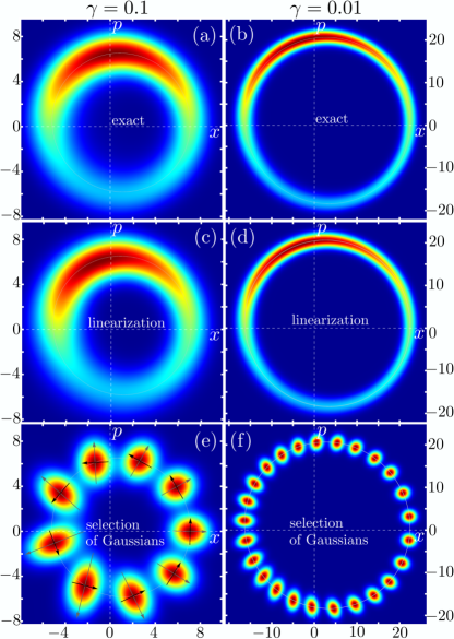
In Fig. 2 we compare the Wigner function (12) with the one obtained by exact simulation CNBnumericsNotes of the master equation (1). We find very good agreement even for relatively large , where quantum fluctuations are still quite relevant, as can be appreciated.
This Wigner function has a very suggestive interpretation, see Fig. 2. First, (10a) tells us that the Gaussian states are centered along the points of the limit cycle’s trajectory, as expected. As for quantum fluctuations, note that the eigenvalues of the covariance matrix are 1 and , which inform us about the variance along the principal axes of the uncertainty ellipse. It is easy to check that the directions of these principal axes follow the vectors and for the 1 and eigenvalues, respectively (see Fig. 2). Hence, the quadrature of the Gaussian state which goes in the direction of (Goldstone mode) carries vacuum fluctuations, which one can trace back to the condition that the method naturally demands. On the other hand, since in principle all physical covariance matrices satisfy (uncertainty principle) CNBbook , this seems to suggest that the quadrature going in the direction of carries fluctuations above the shot noise limit. While this is indeed the case for the VdP oscillator studied here, our experience with other nonlinear systems CNBthesis tells us that we could find (squeezing below shot noise) without violating the uncertainty principle. This is because the two quadratures of each Gaussian state are not conjugate variables, but they are both conjugate to the diffusing variable CNBthesis , which is completely undetermined in the steady state.
Conclusions. In this Letter we have introduced a linearization method capable of dealing with quantum nonlinear systems in the regime where they show spontaneous limit-cycle formation. The technique keeps the simplicity of standard linearization around stationary solutions. It requires finding the fundamental matrix of the Floquet method over a period of the cycle by solving a linear initial value problem with time-periodic coefficients. Only two equations are added with each mode that is introduced in the problem, giving the method a linear scaling with the size of the system that makes it suitable for complex driven-dissipative many-body problems such as optomechanical arrays Arrays1 ; Arrays2 ; Arrays3 ; Arrays4 ; ArraysWeiss . Moreover, the linearity of the equations should give efficient access also to dynamical objects such as multi-time correlation functions, which are of crucial relevance for experiments GardinerZoller ; Carmichael1 ; CarmichaelBook2 ; GardinerZollerI and the emergent field of quantum synchronization Lorch16 ; Lee13 ; Walter14 ; Weiss17 ; Walter15 ; Mari13 .
Acknowledgements.
We thank Florian Marquardt for important suggestions and comments. Our work also benefited from discussions with Alessandro Farace, Alejandro González-Tudela, and Eugenio Roldán. This work was supported by the ERC starting grant OPTOMECH, and by the Ministerio de Economa y Competitividad of the Spanish Government and the European Union FEDER through project FIS2014-60715-P.References
- (1) J. P. Dowling and G. J. Milburn, Phil. Trans. R. Soc. A 361, 3655 (2003).
- (2) M. Benito, C. Sánchez Muñoz, and C. Navarrete-Benlloch, Phys. Rev. A 93, 023846 (2016).
- (3) C. W. Gardiner and P. Zoller, Quantum Noise (Springer-Verlag, Berlin, Heidelberg, 2004).
- (4) C. Gardiner and P. Zoller, The quantum world of ultra-cold atoms and light, Book I (Imperial College Press, London, 2014)
- (5) H.-P. Breuer and F. Petruccione, The Theory of Open Quantum Systems (Oxford University Press, New York, 2002).
- (6) H. J. Carmichael, Statistical Methods in Quantum Optics 1 (Springer-Verlag, Berlin, Heidelberg, 2002).
- (7) P. D. Drummond, K. J. McNeil, and D. F. Walls, J. Mod. Opt. 28, 211 (1981).
- (8) L. A. Lugiato and G. Strini, Opt. Commun. 41, 67 (1981).
- (9) C. Navarrete-Benlloch, E. Roldán, Y. Chang, and T. Shi, Opt. Express 22, 024010 (2014).
- (10) S. H. Strogatz, Nonlinear Dynamics and Chaos (Perseus Books, Reading, 1994).
- (11) R. Grimshaw, Nonlinear ordinary differential equations (Blackwell Scientific, London, 1990).
- (12) I. Perez-Arjona, E. Roldán, and G. J. de Valcárcel, Europhys. Lett. 74, 247 (2006).
- (13) I. Párez-Arjona, E. Roldán, and G. J. de Valcárcel, Phys. Rev. A 75, 063802 (2007).
- (14) C. Navarrete-Benlloch, E. Roldán, and G. J. de Valcárcel, Phys. Rev. Lett. 100, 203601 (2008).
- (15) C. Navarrete-Benlloch, A. Romanelli, E. Roldán, and G. J. de Valcárcel, Phys. Rev. A 81, 043829 (2010).
- (16) Carlos Navarrete-Benlloch, Contributions to the quantum optics of multi-mode optical parametric oscillators (PhD thesis, 2011); arXiv:1504.05917.
- (17) A. S. Lane, M. D. Reid, and D. F. Walls, Phys. Rev. A 38, 788 (1988).
- (18) M. D. Reid and P. D. Drummond, Phys. Rev. Lett. 60, 2731 (1988).
- (19) M. D. Reid and P. D. Drummond, Phys. Rev. A 40, 4493 (1989).
- (20) F. V. Garcia-Ferrer, C. Navarrete-Benlloch, G. J. de Valcárcel, and E. Roldán, IEEE J. Quantum Electron. 45, 1404 (2009).
- (21) F. V. Garcia-Ferrer, C. Navarrete-Benlloch, G. J. de Valcárcel, and E. Roldán, Opt. Lett. 35, 2194 (2010).
- (22) S. Walter, A. Nunnenkamp, and C. Bruder, Phys. Rev. Lett. 112, 094102 (2014).
- (23) T. Weiss, S. Walter, and F. Marquardt, Phys. Rev. A 95, 041802(R) (2017).
- (24) N. Lörch, E. Amitai, A. Nunnenkamp, and C. Bruder, Phys. Rev. Lett. 117, 073601 (2016).
- (25) J. Qian, A. Clerk, K. Hammerer, and F. Marquardt, Phys. Rev. Lett. 109, 253601 (2012).
- (26) N. Lörch, J. Qian, A. Clerk, F. Marquardt, and K. Hammerer, Phys. Rev. X 4, 011015 (2014).
- (27) G. Heinrich, M. Ludwig, J. Qian, B. Kubala, F. Marquardt, Phys. Rev. Lett. 107, 043603 (2011).
- (28) M. Ludwig and F. Marquardt, Phys. Rev. Lett. 111, 073603 (2013).
- (29) R. Lauter, C. Brendel, S. J. M. Habraken, and F. Marquardt, Phys. Rev. E 92, 012902 (2015).
- (30) T. Weiss, A. Kronwald and F. Marquardt, New Journal of Physics 18, 013043 (2016)
- (31) R. Lauter, A. Mitra, F. Marquardt, arXiv:1607.03696 (2016).
- (32) W. P. Schleich, Quantum optics in phase space (Wiley-VCH, 2001).
- (33) P. D. Drummond and C. W. Gardiner, J. Phys. A: Math. Gen. 13, 2353 (1980).
- (34) H. J. Carmichael, Statistical Methods in Quantum Optics 2 (Springer-Verlag, Berlin, 2008).
- (35) C. W. Gardiner, Stochastic Methods: A Handbook for the Natural and Social Sciences, 4 Ed. (Springer-Verlag, Berlin, 2009)
- (36) See the supplemental material, where we derive the stochastic equations of the system, prove the relevant properties of the Floquet eigensystem, and review the phase diagram of the driven VdP oscillator in the classical limit.
- (37) E. A. Coddington and N. Levinson, Theory of Ordinary Differential Equations (McGraw-Hill, New York, 1955).
- (38) C. Navarrete-Benlloch, An Introduction to the Formalism of Quantum Information with Continuous Variables (Morgan & Claypool and IOP, Bristol, 2015).
- (39) C. Navarrete-Benlloch, Open systems dynamics. Simulating master equations in the computer; arXiv:1504.05266.
- (40) T. E. Lee and H. R. Sadeghpour, Phys. Rev. Lett. 111, 234101 (2013).
- (41) S. Walter, A. Nunnenkamp, and C. Bruder, Ann. Phys. 527, 131 (2015).
- (42) A. Mari, A. Farace, N. Didier, V. Giovannetti, and R. Fazio, Phys. Rev. Lett. 111, 103605 (2013).
Supplemental material
This supplemental material is divided in three sections. In the first one we derive the stochastic Langevin equations associated with the master equation of the driven Van der Pol oscillator, and proceed to their linearization. The second section is devoted to proving the properties of the Floquet eigensystem that we introduced in the main text. In the last section we provide a detailed overview of the phase diagram of the Van der Pol oscillator in the classical limit.
I. Derivation of the stochastic equations
The positive P representation of a (single-mode) state is defined by Drummond80 ; CarmichaelBook2 ; GardinerZoller ; GardinerZollerI
| (13) |
with . The distribution can always be chosen as a well behaved positive distribution (see below), what is accomplished at the expense of doubling the phase space of the oscillator, since and are two independent complex variables. Moments in normal order can be evaluated as Drummond80 ; CarmichaelBook2 ; GardinerZoller ; GardinerZollerI
| (14) |
The master equation can be turned into a Fokker-Planck equation for the distribution as follows. First, we introduce (13) in the master equation, Eq. (1) of the main text in our case, and use the properties
| (15) |
leading to an equation of the form
| (16) |
Here and are the components of the drift vector and the diffusion matrix, respectively, which in our case are found to be
| (17c) | ||||
| (17f) | ||||
Note that the analyticity of gives us certain freedom to choose how the the complex derivatives and act on it, what can be used to always get a positive semidefinite diffusion matrix CNBthesis ; Drummond80 . Integrating by parts the right-hand side of Eq. (16), and neglecting boundary terms under the physical assumption that the distribution decays fast enough, we obtain the Fokker-Planck equation
| (18) |
This equation is equivalent to the following stochastic Langevin equations Drummond80 ; CarmichaelBook2 ; GardinerZoller ; GardinerZollerI ; GardinerBook
| (19) |
where is a matrix called the noise matrix which satisfies , and a vector whose components are independent real white Gaussian noises ( can be chosen at will, see below). Given the solution as a functional of the noises, the equivalence must be understood in a statistical sense as
| (20) |
that is, averaging over the distribution equals averaging over stochastic realizations. In the following we remove the “stochastic” label from the average, since the context will never allow confusing it with quantum expectation values of operators.
As mentioned above, the “internal” dimension of the noise matrix is arbitrary in expression (19). In general, it is possible to find a square noise matrix ( in our case), but sometimes it is simpler (or even more physical) to work with . In particular, in our case, we choose to work with the noise matrix
| (21) |
leading to the Langevin equations
| (22a) | ||||
| (22b) | ||||
where , , and are independent white Gaussian noises (real the first two, and complex the last one), that is, they have zero average and
| (23) |
are their only nonzero two-time correlators.
It is finally interesting to rewrite the equations in terms of new rescaled variables and , which read
| (24a) | ||||
| (24b) | ||||
These are the equations that we provided in Eqs. (2) of the main text. We took them as a starting point to present the linearization technique, which we show in detail next.
The general linearization technique for dissipative systems affected by spontaneous breaking of a continuous symmetry starts by applying the symmetry transformation to the system, but with a parameter that is allowed to vary in time CNBthesis . In the present case, the method finds the additional difficulty that the symmetry transformation is a shift in time , and if the parameter is to depend on time, the shift must be applied on it as well. Technically, this makes it an infinitely-iterated function , which makes the derivation more elaborate than in previous systems CNBthesis . The (time-shifted) stochastic amplitudes are expanded as the classical limit cycle plus some small quantum that can be assumed to be small,
| (25) |
where we have omitted the time dependence of for ease of notation.
When plugging this expressions into the stochastic Langevin equations (24), it is important to keep in mind that the derivative of can be assumed small, since the method tells us self-consistently that they are directly proportional to quantum noise, see the paragraph before Eq. (8) in the main text. This means that we can approximate
| (26) |
and therefore
| (27) |
and similarly for , where in the last line we have assumed that the fluctuations and related derivatives are small. Introducing these expansions into Eqs. (24) evaluated at , and keeping terms linear in noises and the small variables mentioned above, we obtain the linearized Langevin equations introduced in Eq. (4) of the main text, but time-shifted by . The last step consists then in shifting the time arguments by , leading to the linearized equations as presented in the main text.
II. Floquet eigensystem
In order to solve the linearized Langevin equations we applied the Floquet method in the main text. In particular, we showed that all the system properties are easy to derive from the Floquet eigensystem, that is, from the eigenvalues and eigenvectors satisfying
| (28a) | ||||
| (28b) | ||||
and the orthogonality conditions . In general, this has to be done numerically, especially since the limit cycle itself does not admit analytic expressions except in special situations. However, we mentioned in the main text a couple of analytic properties of the eigensystem that we prove in this section.
Since these properties are not specific to the Van der Pol oscillator, but general for any single-mode problem, let us consider a completely general single-mode limit cycle satisfying the equation
| (29) |
with associated linear stability matrix
| (30) |
It is convenient to define the vector . Its first derivative satisfies the equation , leading to a second derivative obeying
| (31) |
The first property we want to prove is the existence of one null eigenvalue, say , with an associated (right) Floquet eigenvector . In order to prove it just note that according to (28) satisfies the equation by construction. On the other hand, since , we also have by virtue of (31). Comparing these two expressions we obtain . This property finds its roots on the Goldstone theorem, and indeed can be proven for an arbitrary number of modes by naturally extending all the definitions.
The other property that we provided in the main text was that the other eigenvalue takes the value , where we define here , with associated (left) Floquet eigenvector
| (32) |
with . The expression for the eigenvalue is readily proven by noticing that for a general Floquet problem, the following property holds GrimshawBook ; CodingtonBook : . Hence, for a single-mode problem we obtain what we are looking for, since there are only two eigenvalues and one of them is 0 as proven above.
To prove that (32) is the corresponding eigenvector we need to work a bit harder. We will proceed by making the ansatz for some real function , and proving that such a function exists. It is convenient to remind ourselves of certain objects that naturally appear in the Floquet method (see the main text for more details). First, the fundamental matrix which satisfies the equation . This matrix defines a constant matrix through , and a periodic matrix . The Floquet eigenvectors are then defined as and , where is the eigensystem of , composed of right and left orthogonal eigenvectors satisfying and . With these definitions at hand, we start by noting that
| (33) |
The time derivative of this expression and our ansatz yields
| (34) |
where we have used that, by definition, the fundamental matrix satisfies . From this expression, we see that can be written as
| (35) |
The next step is obtaining following a different path. Let us define the matrix
| (36) |
which allows us to write
| (37) |
Next, we exploit the structure of any single-mode linear stability matrix (30) to write
| (38) |
which combined with the previous result leads to
| (39) |
Finally, comparing (35) and (39), and using the expression that we found for we get
| (40) |
which shows that there is a indeed a solution for the ansatz function,
| (41) |
where we have taken for definiteness. This completes the proof of (32).
III. Phase diagram in the classical limit
In this section we analyze in detail the properties of the driven Van der Pol oscillator in the classical limit. In the main text, we argued that the classical limit corresponds to in the stochastic Langevin equations. Let us show here, for completeness, that these are indeed the equations that are obtained by assuming the state of the system to be coherent at all times, , with a time-dependent amplitude that will be our classical variable (normalized to for convenience). In order to find an evolution equation for , we proceed as follows. Using the master equation (1) of the main text, the expectation value of any operator is shown to evolve according to
| (42) |
Applied to the annihilation operator and using the coherent state ansatz, such that , we obtain the equation of motion
| (43) |
which is precisely the one we introduced in the main text and coincides with the stochastic Langevin equations in the limit. Note that there are only two parameters in this equation, which fully characterize the phase diagram in this limit, as we show in Fig. 3 (see below for the meaning of ).
Depending on the parameters, the asymptotic (long-time term) solutions of this equation may be time independent (stationary) or dependent (limit cycles). In order to identify when these different regimes happen, we first find the stationary asymptotic solutions and study their stability. Let us write the amplitude as , with and , which introduced in the equation of motion (43) leads to the steady-state equation , or the equation for the oscillator intensity
| (44) |
from which the phase is recovered as . This equation may possess one or several real and positive solutions, depending on the parameters. In order to determine when each of these possibilities occur, we simply determine the turning points of the S-shaped curve shown in Figs. 4. These can be found as the extrema of ,
| (45) |
Hence, we see that these points only exist when . The values of the injection corresponding to these intensities can be written as
| (46) |
For injections between these two values, we then find three-valued intensities.
Let’s now consider the stability of these solutions GrimshawBook ; StrogatzBook . It is convenient to take the intensity as a parameter rather than , since the latter is uniquely determined from the former through Eq. (44), and not the other way around. In order to analyze the stability of a stationary solution , we write the amplitudes as , and consider terms up to linear order in the evolution equation (43). Defining the vector , this provides an evolution equation of the form , where the linear stability matrix reads
| (47) |
with characteristic polynomial
| (48) |
and therefore eigenvalues
| (49) |
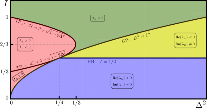
Whenever the real part of at least one of these eigenvalues is positive, the corresponding solution will be unstable. The points of the parameter space where the real part of an eigenvalue is zero are known as instabilities or bifurcations StrogatzBook . It is customary to start checking the simplest instabilities, those where the imaginary part of the corresponding eigenvalue is zero as well, which we denote by static instabilities. In our case, it is readily shown that the turning points are the only static instabilities (see the curves marked as TP± in Fig. 3). On the other hand, the instabilities can appear in eigenvalues with nonzero imaginary parts, in which case we talk about Hopf bifurcations StrogatzBook . In our case, imaginary parts in the eigenvalues (49) appear only when (see the curve marked as UP111UP stands for “underdamped phase” oscillations, a name that will get meaning later, when we show that the region corresponds precisely to this regime of motion. in Fig. 3). We then find a Hopf bifurcation at (see the curve marked as HB in Fig. 3). A careful analysis of the signs of the real part of the eigenvalues in between these instability curves leads to the phase diagram shown in Fig. 3. Note that we are able to draw such a simple (but rich) phase diagram because we are dealing with a single harmonic mode whose eigenvalues depend only on two parameters ( and ) and have simple analytic expressions.
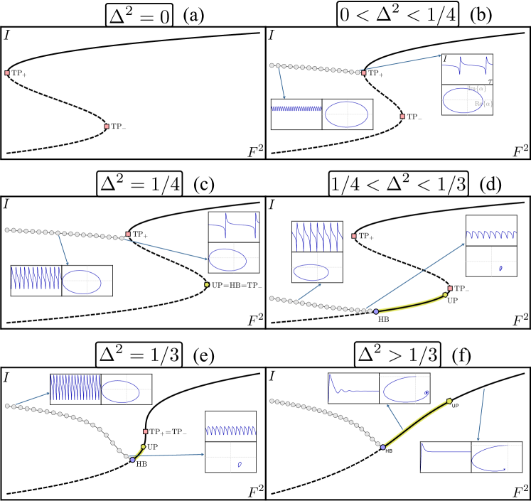
It is also interesting to understand the behaviour of the oscillator’s amplitude as a function of the injection in the different regions of the phase diagram, in particular for different values of . This is what we can see in Fig. 4:
It can be appreciated that for only the upper branch is stable, and increases monotonically with the injection from at (Fig. 4a). Hence, the oscillator’s amplitude has a unique stationary response for all injections, since the drive is in resonance with the oscillator’s natural frequency.
When (Fig. 4b) the upper turning point departs from . The asymptotic solution corresponds then to a limit cycle for and to a stationary solution in the upper branch for . The physical interpretation is clear: as soon as the drive is detuned, synchronization of the oscillator’s oscillations to the drive requires a minimum value of the injection in order to work. Note that for , the limit cycles are of the trivial form , which simply means that the amplitude oscillates at the natural frequency of the oscillator.
At (Fig. 4c), both the Hopf bifurcation HB and the UP point appear precisely at the lower turning point. If the detuning is made larger, specifically (Fig. 4d), both the Hopf bifurcation and the UP point are located somewhere along the lower branch of the S-shaped curve, the former always below the latter. The portion of the lower branch in between HB and TP- becomes stable, with underdamped phase oscillations in between HB and UP. We observe that in this regime there is coexistence between the stationary solutions of the upper branch, and either limit cycles connected to the HB from or stationary solutions in the lower branch.
For the turning points coalesce (Fig. 4e), and therefore for the steady-state curve is no longer S-shaped, but increases monotonically with the injection as shown in Fig. 4f. We then identify a unique behaviour of the amplitude for each value of the injection which can correspond to limit cycles, underdamped phase oscillations, or overdamped phase oscillations.
It is interesting to note the different ways in which the limit cycles converge to the stationary solutions in the different regimes, which is what the insets allow us to discuss. In particular, when the limit cycles connect with a static instability (such as in Figs. 4b and c, where they connect with the upper turning point), their periodic pattern has a longer stationary plateau the closer we get to the instability, eventually reaching an infinite duration. On the other hand, when the limit cycles connect with a Hopf instability (such as in Figs. 4d, e, and f), their oscillation frequency becomes closer to the closer they are to the instability, while at the same time their oscillation amplitude becomes smaller and smaller, eventually reaching zero.
Hence, we see that the VdP oscillator has a rich dynamical behaviour in the classical limit.
One final thing left to prove is that, as mentioned above above, the region where the eigenvalues are complex () coincides with the region of underdamped phase oscillations. In order to show this, let us write the oscillator’s amplitude in terms of intensity and phase fluctuations around the steady state as
| (50) |
so that the amplitude fluctuations can be written as . Using now the form of the linear stability matrix (47), we then get from the real and imaginary parts of the linear system for the fluctuations the following phase and amplitude equations
| (51a) | ||||
| (51b) | ||||
These first order differential equations can be easily recasted as the following second order differential equation for the phase fluctuations
| (52) |
which is the equation of a damped harmonic oscillator. Hence, the condition for underdamped phase oscillations is , leading to , just as we wanted to prove.