Penalized bias reduction in extreme value estimation for censored Pareto-type data, and long-tailed insurance applications

J. Beirlant a,b111Corresponding author: Jan Beirlant, KU Leuven, Dept of Mathematics, Celestijnenlaan 200B, 3001 Heverlee, Belgium; Email: jan.beirlant@kuleuven.be , G. Maribe b, A. Versterb
a Dept. of Mathematics, LStat and LRisk, KU Leuven
b Dept. of Mathematical Statistics and Actuarial Science, University of the Free State
Abstract

The subject of tail estimation for randomly censored data from a heavy tailed distribution receives growing attention, motivated by applications for instance in actuarial statistics. The bias of the available estimators of the extreme value index can be substantial and depends strongly on the amount of censoring. We review the available estimators, propose a new bias reduced estimator, and show how shrinkage estimation can help to keep the MSE under control. A bootstrap algorithm is proposed to construct confidence intervals. We compare these new proposals with the existing estimators through simulation. We conclude this paper with a detailed study of a long-tailed car insurance portfolio, which typically exhibit heavy censoring.

Keywords: Extreme value index; Pareto-type; Tail estimation; Random censoring; Bias reduction.

1 Introduction

Extreme value analysis under random right censoring is becoming more popular with applications for example in survival analysis, reliability and insurance. For instance, in certain long-tailed insurance products, such as car liability insurance, long developments of claims are encountered. At evaluation of the portfolio a large proportion of the claims are then not fully developed and hence are censored.

In the setting of random right censoring the variable of interest X𝑋X with distribution function (df) F𝐹F can be censored by a random variable C𝐢C with df G𝐺G. Moreover observations of X𝑋X and C𝐢C are assumed to be independent. One then observes Z=min⁑(X,C)𝑍𝑋𝐢Z=\min(X,C) with df H𝐻H satisfying 1βˆ’H=(1βˆ’F)​(1βˆ’G)1𝐻1𝐹1𝐺1-H=(1-F)(1-G), jointly with the indicator Ξ΄=1(X≀C)𝛿subscript1𝑋𝐢\delta=1_{(X\leq C)} which equals 1 if the observation Z𝑍Z is non-censored. Here we assume that X𝑋X and C𝐢C both are Pareto-type distributed with extreme value index (EVI) Ξ³1>0subscript𝛾10\gamma_{1}>0 and Ξ³2>0subscript𝛾20\gamma_{2}>0, i.e.

F¯​(x)=1βˆ’F​(x)=xβˆ’1/Ξ³1​ℓ1​(x)​ and ​G¯​(y)=1βˆ’G​(y)=yβˆ’1/Ξ³2​ℓ2​(y),x,y>1,formulae-sequence¯𝐹π‘₯1𝐹π‘₯superscriptπ‘₯1subscript𝛾1subscriptβ„“1π‘₯Β and ¯𝐺𝑦1𝐺𝑦superscript𝑦1subscript𝛾2subscriptβ„“2𝑦π‘₯𝑦1\bar{F}(x)=1-F(x)=x^{-1/\gamma_{1}}\ell_{1}(x)\mbox{ and }\bar{G}(y)=1-G(y)=y^{-1/\gamma_{2}}\ell_{2}(y),\;\;x,y>1,

where both β„“1,β„“2subscriptβ„“1subscriptβ„“2\ell_{1},\ell_{2} are slowly varying at infinity:

β„“j​(t​x)/β„“j​(t)β†’tβ†’βˆž1,Β for every ​x>1​(j=1,2).formulae-sequencesubscript→→𝑑subscriptℓ𝑗𝑑π‘₯subscriptℓ𝑗𝑑1Β for everyΒ π‘₯1𝑗12\ell_{j}(tx)/\ell_{j}(t)\to_{t\to\infty}1,\;\;\mbox{ for every }x>1\;\;(j=1,2).

Note that 1βˆ’H1𝐻1-H then also belongs to the domain of attraction of an extreme value distribution with positive EVI Ξ³=Ξ³1​γ2Ξ³1+Ξ³2𝛾subscript𝛾1subscript𝛾2subscript𝛾1subscript𝛾2\gamma={{\gamma_{1}\gamma_{2}}\over{\gamma_{1}+\gamma_{2}}}. Of course, the smaller Ξ³2/Ξ³1subscript𝛾2subscript𝛾1\gamma_{2}/\gamma_{1} the heavier the censoring will be. In long-tailed insurance applications as discussed above, the proportion of censored data can well be larger than 50%, so that the situation Ξ³2<Ξ³1subscript𝛾2subscript𝛾1\gamma_{2}<\gamma_{1} is then most relevant.

In this paper we discuss the estimation of Ξ³1subscript𝛾1\gamma_{1} based on independent and identically distributed (i.i.d.) observations (Zi,Ξ΄i)subscript𝑍𝑖subscript𝛿𝑖(Z_{i},\delta_{i}) (i=1,…,n𝑖1…𝑛i=1,\ldots,n) with Zi=min⁑(Xi,Ci)subscript𝑍𝑖subscript𝑋𝑖subscript𝐢𝑖Z_{i}=\min(X_{i},C_{i}) and Ξ΄i=1(Xi≀Ci)subscript𝛿𝑖subscript1subscript𝑋𝑖subscript𝐢𝑖\delta_{i}=1_{(X_{i}\leq C_{i})}, where (Xi,Ci)subscript𝑋𝑖subscript𝐢𝑖(X_{i},C_{i}) (i=1,…,n𝑖1…𝑛i=1,\ldots,n) are i.i.d. random variables from (F,G)𝐹𝐺(F,G). In the next section we review the available estimators for Ξ³1subscript𝛾1\gamma_{1} that were published in the literature. In Section 3 we propose a new bias reduced estimator which is based on an estimator proposed by Worms and Worms (2014). Moreover we show how shrinkage estimation, as introduced in Beirlant et al. (2017) in the non-censoring case, can also be used in the censoring context. In Section 4 a parametric bootstrap algorithm is proposed in order to construct confidence intervals for Ξ³1subscript𝛾1\gamma_{1}. We then report on a simulation study involving all available estimators and the proposed bootstrap algorithm. Finally we make a detailed study of a motor third party liability (MTPL) case study.

2 A review of estimators of Ξ³1subscript𝛾1\gamma_{1}

In case there is no censoring (i.e. Ξ³2=∞subscript𝛾2\gamma_{2}=\infty and 1βˆ’H=1βˆ’F1𝐻1𝐹1-H=1-F), the Hill (1975) estimator is the benchmark estimator for Ξ³1=Ξ³subscript𝛾1𝛾\gamma_{1}=\gamma. Denoting the ordered Z𝑍Z data by Z1,n≀Z2,n≀…≀Zn,nsubscript𝑍1𝑛subscript𝑍2𝑛…subscript𝑍𝑛𝑛Z_{1,n}\leq Z_{2,n}\leq\ldots\leq Z_{n,n} this estimator is given by

Ξ³^Z,kH=1kβ€‹βˆ‘j=1klog⁑Znβˆ’j+1,nZnβˆ’k,n.superscriptsubscript^π›Ύπ‘π‘˜π»1π‘˜superscriptsubscript𝑗1π‘˜subscript𝑍𝑛𝑗1𝑛subscriptπ‘π‘›π‘˜π‘›\hat{\gamma}_{Z,k}^{H}={1\over k}\sum_{j=1}^{k}\log{Z_{n-j+1,n}\over Z_{n-k,n}}.

This estimator follows using maximum likelihood when approximating the distribution of the peaks Z/t𝑍𝑑Z/t over a threshold t𝑑t, given Z>t𝑍𝑑Z>t, by a simple Pareto distribution with density yβ†¦Ξ³βˆ’1​yβˆ’Ξ³βˆ’1βˆ’1maps-to𝑦superscript𝛾1superscript𝑦superscript𝛾11y\mapsto\gamma^{-1}y^{-\gamma^{-1}-1}, and taking a top order statistic Znβˆ’k,nsubscriptπ‘π‘›π‘˜π‘›Z_{n-k,n} as a threshold t𝑑t.
It can also be found back by estimating the functional

Lt:=𝔼​(log⁑Zβˆ’log⁑t​|Z>​t)=∫1∞F¯​(u​t)F¯​(t)​d​uu,assignsubscript𝐿𝑑𝔼𝑍𝑑ket𝑍𝑑superscriptsubscript1¯𝐹𝑒𝑑¯𝐹𝑑𝑑𝑒𝑒L_{t}:=\mathbb{E}(\log Z-\log t|Z>t)=\int_{1}^{\infty}{\bar{F}(ut)\over\bar{F}(t)}{du\over u}, (1)

which tends to the extreme value index γ𝛾\gamma of Z𝑍Z as tβ†’βˆžβ†’π‘‘t\to\infty. In (1) F¯¯𝐹\bar{F} is estimated by the empirical survival function 1βˆ’F^n1subscript^𝐹𝑛1-\hat{F}_{n}, again using Znβˆ’k,nsubscriptπ‘π‘›π‘˜π‘›Z_{n-k,n} as a threshold t𝑑t. This leads to an alternative writing of Ξ³^Z,kHsuperscriptsubscript^π›Ύπ‘π‘˜π»\hat{\gamma}_{Z,k}^{H} by partial summation:

Ξ³^Z,k(H)=1kβ€‹βˆ‘j=1kj​(log⁑Znβˆ’j+1,nβˆ’log⁑Znβˆ’j,n).superscriptsubscript^π›Ύπ‘π‘˜π»1π‘˜superscriptsubscript𝑗1π‘˜π‘—subscript𝑍𝑛𝑗1𝑛subscript𝑍𝑛𝑗𝑛\hat{\gamma}_{Z,k}^{(H)}={1\over k}\sum_{j=1}^{k}j(\log Z_{n-j+1,n}-\log Z_{n-j,n}).

While both approaches yield the same estimator in the non-censoring case this is no longer the case under random censoring.

  • β€’

    Beirlant et al. (2007) proposed the following estimator of Ξ³1subscript𝛾1\gamma_{1} using the maximum likelihood approach:

    Ξ³^1,k(H)=Ξ³^Z,k(H)p^k,superscriptsubscript^𝛾1π‘˜π»superscriptsubscript^π›Ύπ‘π‘˜π»subscript^π‘π‘˜\hat{\gamma}_{1,k}^{(H)}={\hat{\gamma}_{Z,k}^{(H)}\over\hat{p}_{k}}, (2)

    with p^k=1kβ€‹βˆ‘j=1kΞ΄nβˆ’j+1,nsubscript^π‘π‘˜1π‘˜superscriptsubscript𝑗1π‘˜subscript𝛿𝑛𝑗1𝑛\hat{p}_{k}={1\over k}\sum_{j=1}^{k}\delta_{n-j+1,n} the proportion of non-censored observations under the largest kπ‘˜k observations of Z𝑍Z, where Ξ΄nβˆ’j+1,nsubscript𝛿𝑛𝑗1𝑛\delta_{n-j+1,n} denotes the δ𝛿\delta indicator attached to Znβˆ’j+1,nsubscript𝑍𝑛𝑗1𝑛Z_{n-j+1,n} (1≀j≀n)1𝑗𝑛(1\leq j\leq n). Indeed, Ξ³^Z,kHsuperscriptsubscript^π›Ύπ‘π‘˜π»\hat{\gamma}_{Z,k}^{H} estimates γ𝛾\gamma while p^ksubscript^π‘π‘˜\hat{p}_{k} is shown to be a consistent estimator of p=Ξ³2/(Ξ³1+Ξ³2)𝑝subscript𝛾2subscript𝛾1subscript𝛾2p=\gamma_{2}/(\gamma_{1}+\gamma_{2}). Einmahl et al. (2008) enhanced the asymptotic analysis of this estimator and generalized this approach by considering any classical EVI estimator Ξ³^Z,k(.)\hat{\gamma}_{Z,k}^{(.)} of γ𝛾\gamma, proposing the estimators Ξ³^1,k(.)=Ξ³^Z,k(.)p^k\hat{\gamma}_{1,k}^{(.)}={\hat{\gamma}_{Z,k}^{(.)}\over\hat{p}_{k}}. See also Gomes and Oliveira (2003), Gomes and Neves (2011), and Brahimi et al. (2015) for other papers in this spirit.

  • β€’

    Worms and Worms (2014) essentially used the second approach estimating (1) by substituting 1βˆ’F1𝐹1-F with the Kaplan-Meier estimator 1βˆ’F^nK​M​(x)=Ξ Zi,n≀x​(1βˆ’1nβˆ’i+1)Ξ΄i,n1subscriptsuperscript^𝐹𝐾𝑀𝑛π‘₯subscriptΞ subscript𝑍𝑖𝑛π‘₯superscript11𝑛𝑖1subscript𝛿𝑖𝑛1-\hat{F}^{KM}_{n}(x)=\Pi_{Z_{i,n}\leq x}\left(1-{1\over n-i+1}\right)^{\delta_{i,n}}, setting 1βˆ’F^nK​M​(Zn,n)=01subscriptsuperscript^𝐹𝐾𝑀𝑛subscript𝑍𝑛𝑛01-\hat{F}^{KM}_{n}(Z_{n,n})=0:

    Ξ³^1,k(W)=βˆ‘j=1k1βˆ’F^nK​M​(Znβˆ’j+1,n)1βˆ’F^nK​M​(Znβˆ’k,n)​(log⁑Znβˆ’j+1,nβˆ’log⁑Znβˆ’j,n).superscriptsubscript^𝛾1π‘˜π‘Šsuperscriptsubscript𝑗1π‘˜1subscriptsuperscript^𝐹𝐾𝑀𝑛subscript𝑍𝑛𝑗1𝑛1subscriptsuperscript^𝐹𝐾𝑀𝑛subscriptπ‘π‘›π‘˜π‘›subscript𝑍𝑛𝑗1𝑛subscript𝑍𝑛𝑗𝑛\hat{\gamma}_{1,k}^{(W)}=\sum_{j=1}^{k}{1-\hat{F}^{KM}_{n}(Z_{n-j+1,n})\over 1-\hat{F}^{KM}_{n}(Z_{n-k,n})}\left(\log Z_{n-j+1,n}-\log Z_{n-j,n}\right). (3)

    Worms and Worms (2014) also introduced

    Ξ³^1,k(K​M)=βˆ‘j=1k1βˆ’F^nK​M​(Znβˆ’j+1,n)1βˆ’F^nK​M​(Znβˆ’k,n)​δnβˆ’j+1,nj​(log⁑Znβˆ’j+1,nβˆ’log⁑Znβˆ’k,n).superscriptsubscript^𝛾1π‘˜πΎπ‘€superscriptsubscript𝑗1π‘˜1subscriptsuperscript^𝐹𝐾𝑀𝑛subscript𝑍𝑛𝑗1𝑛1subscriptsuperscript^𝐹𝐾𝑀𝑛subscriptπ‘π‘›π‘˜π‘›subscript𝛿𝑛𝑗1𝑛𝑗subscript𝑍𝑛𝑗1𝑛subscriptπ‘π‘›π‘˜π‘›\hat{\gamma}_{1,k}^{(KM)}=\sum_{j=1}^{k}{1-\hat{F}^{KM}_{n}(Z_{n-j+1,n})\over 1-\hat{F}^{KM}_{n}(Z_{n-k,n})}{\delta_{n-j+1,n}\over j}\left(\log Z_{n-j+1,n}-\log Z_{n-k,n}\right). (4)

    Through simulations the estimator Ξ³^1,k(W)subscriptsuperscript^π›Ύπ‘Š1π‘˜\hat{\gamma}^{(W)}_{1,k} was found to have the best RMSE behaviour for smaller values of kπ‘˜k. Below we will then concentrate on Ξ³^1,k(W)superscriptsubscript^𝛾1π‘˜π‘Š\hat{\gamma}_{1,k}^{(W)}. Unfortunately, the asymptotic distribution of Ξ³^1,k(W)superscriptsubscript^𝛾1π‘˜π‘Š\hat{\gamma}_{1,k}^{(W)} is not known up to now. The asymptotic normality of a fixed threshold version of Ξ³^1,k(K​M)superscriptsubscript^𝛾1π‘˜πΎπ‘€\hat{\gamma}_{1,k}^{(KM)} can be derived from Worms and Worms (2017) in case Ξ³1<Ξ³2subscript𝛾1subscript𝛾2\gamma_{1}<\gamma_{2}. Brahimi et al. (2016) consider closely related estimators but also considered asymptotic results in case Ξ³1<Ξ³2subscript𝛾1subscript𝛾2\gamma_{1}<\gamma_{2} or p>1/2𝑝12p>1/2.

  • β€’

    In an objective Bayesian approach (see Zellner, 1971), Ameraoui et al. (2016) recently proposed several other estimators. They considered the maximum posterior (m) and the mean posterior (e) estimators of the posterior density of Ξ³1subscript𝛾1\gamma_{1}. The maximal data information (M) prior and a conjugate gamma prior with parameters (a,b)π‘Žπ‘(a,b) were considered. It was also shown that Jeffreys prior lead to special cases of the conjugate prior estimators setting a=b=0π‘Žπ‘0a=b=0. This then leads to the following estimators:

    Ξ³^1,k(m,M)superscriptsubscript^𝛾1π‘˜π‘šπ‘€\displaystyle\hat{\gamma}_{1,k}^{(m,M)} =\displaystyle= 2​k​γ^Z,k(H)1+k​p^k+(1+k​p^k)2+4​k​γ^Z,k(H),2π‘˜superscriptsubscript^π›Ύπ‘π‘˜π»1π‘˜subscript^π‘π‘˜superscript1π‘˜subscript^π‘π‘˜24π‘˜superscriptsubscript^π›Ύπ‘π‘˜π»\displaystyle{2k\hat{\gamma}_{Z,k}^{(H)}\over 1+k\hat{p}_{k}+\sqrt{(1+k\hat{p}_{k})^{2}+4k\hat{\gamma}_{Z,k}^{(H)}}}, (5)
    Ξ³^1,k(e,a,b)superscriptsubscript^𝛾1π‘˜π‘’π‘Žπ‘\displaystyle\hat{\gamma}_{1,k}^{(e,a,b)} =\displaystyle= k​γ^Z,k(H)+bk​p^k+a,π‘˜superscriptsubscript^π›Ύπ‘π‘˜π»π‘π‘˜subscript^π‘π‘˜π‘Ž\displaystyle{k\hat{\gamma}_{Z,k}^{(H)}+b\over k\hat{p}_{k}+a}, (6)
    Ξ³^1,k(m,a,b)superscriptsubscript^𝛾1π‘˜π‘šπ‘Žπ‘\displaystyle\hat{\gamma}_{1,k}^{(m,a,b)} =\displaystyle= k​γ^Z,k(H)+bk​p^k+aβˆ’1.π‘˜superscriptsubscript^π›Ύπ‘π‘˜π»π‘π‘˜subscript^π‘π‘˜π‘Ž1\displaystyle{k\hat{\gamma}_{Z,k}^{(H)}+b\over k\hat{p}_{k}+a-1}. (7)

It is well-known that extreme value estimators often suffer from severe bias. In the random censoring case Einmahl et al. (2008) first derived the asymptotic bias of Ξ³^1,k(H)superscriptsubscript^𝛾1π‘˜π»\hat{\gamma}_{1,k}^{(H)}, which was further detailed in Beirlant et al. (2016) under more specific assumptions on the slowly varying functions β„“1subscriptβ„“1\ell_{1} and β„“2subscriptβ„“2\ell_{2}, which are commonly proposed in extreme value statistics:

1βˆ’F​(x)1𝐹π‘₯\displaystyle 1-F(x) =\displaystyle= C1​xβˆ’1/Ξ³1​(1+D1​xβˆ’Ξ²1​(1+o​(1))),xβ†’βˆž,β†’subscript𝐢1superscriptπ‘₯1subscript𝛾11subscript𝐷1superscriptπ‘₯subscript𝛽11π‘œ1π‘₯\displaystyle C_{1}{x^{-1/\gamma_{1}}}(1+D_{1}x^{-\beta_{1}}(1+o(1))),\;x\to\infty,
1βˆ’G​(y)1𝐺𝑦\displaystyle 1-G(y) =\displaystyle= C2​yβˆ’1/Ξ³2​(1+D2​xβˆ’Ξ²2​(1+o​(1))),yβ†’βˆž,β†’subscript𝐢2superscript𝑦1subscript𝛾21subscript𝐷2superscriptπ‘₯subscript𝛽21π‘œ1𝑦\displaystyle C_{2}{y^{-1/\gamma_{2}}}(1+D_{2}x^{-\beta_{2}}(1+o(1))),\;y\to\infty,

where Ξ²1,Ξ²2,C1,C2subscript𝛽1subscript𝛽2subscript𝐢1subscript𝐢2\beta_{1},\beta_{2},C_{1},C_{2} are positive constants and D1,D2subscript𝐷1subscript𝐷2D_{1},D_{2} are real constants. Taking the bias of the Hill estimator Ξ³^Z,k(H)subscriptsuperscript^π›Ύπ»π‘π‘˜\hat{\gamma}^{(H)}_{Z,k} as a reference, it was observed that especially when Ξ²1≀β2subscript𝛽1subscript𝛽2\beta_{1}\leq\beta_{2} the bias of Ξ³^1,k(H)superscriptsubscript^𝛾1π‘˜π»\hat{\gamma}_{1,k}^{(H)} increases with decreasing value of p𝑝p, i.e. for smaller Ξ³2/Ξ³1subscript𝛾2subscript𝛾1\gamma_{2}/\gamma_{1}. Within the maximum likelihood approach, a bias reduced estimator was then proposed for the censoring case following the technique from Beirlant et al. (2009) where the distribution of the excesses X/t​|X>​t𝑋𝑑ket𝑋𝑑X/t|X>t is approximated by the extended Pareto (EP) distribution with df ℙ​(Y≀y)=1βˆ’(y​{1+ΞΊt​(1βˆ’yβˆ’Ξ²1)})βˆ’1/Ξ³1β„™π‘Œπ‘¦1superscript𝑦1subscriptπœ…π‘‘1superscript𝑦subscript𝛽11subscript𝛾1\mathbb{P}(Y\leq y)=1-(y\{1+\kappa_{t}(1-y^{-\beta_{1}})\})^{-1/\gamma_{1}} where ΞΊt=Ξ³1​D1​tβˆ’Ξ²1​(1+o​(1))subscriptπœ…π‘‘subscript𝛾1subscript𝐷1superscript𝑑subscript𝛽11π‘œ1\kappa_{t}=\gamma_{1}D_{1}t^{-\beta_{1}}(1+o(1)) as tβ†’βˆžβ†’π‘‘t\to\infty. The resulting estimator is given by

Ξ³^1,k(E​P)=Ξ³^1,k(H)+CΞ³^1,k(H),Ξ²βˆ—β€‹HZ,k(βˆ’Ξ²βˆ—)p^k​{HZ,k(βˆ’Ξ²βˆ—)βˆ’Ξ³^1,k(H)​EZ,k(c)​(βˆ’Ξ²βˆ—)}superscriptsubscript^𝛾1π‘˜πΈπ‘ƒsuperscriptsubscript^𝛾1π‘˜π»subscript𝐢superscriptsubscript^𝛾1π‘˜π»subscript𝛽superscriptsubscriptπ»π‘π‘˜subscript𝛽subscript^π‘π‘˜superscriptsubscriptπ»π‘π‘˜subscript𝛽superscriptsubscript^𝛾1π‘˜π»superscriptsubscriptπΈπ‘π‘˜π‘subscript𝛽\hat{\gamma}_{1,k}^{(EP)}=\hat{\gamma}_{1,k}^{(H)}+C_{\hat{\gamma}_{1,k}^{(H)},\beta_{*}}{H_{Z,k}^{(-\beta_{*})}\over\hat{p}_{k}}\left\{H_{Z,k}^{(-\beta_{*})}-\hat{\gamma}_{1,k}^{(H)}E_{Z,k}^{(c)}(-\beta_{*})\right\} (8)

where, Ξ²βˆ—=min⁑(Ξ²1,Ξ²2)subscript𝛽subscript𝛽1subscript𝛽2\beta_{*}=\min(\beta_{1},\beta_{2}) and

HZ,k(βˆ’Ξ²βˆ—)superscriptsubscriptπ»π‘π‘˜subscript𝛽\displaystyle H_{Z,k}^{(-\beta_{*})} =\displaystyle= 1Ξ²βˆ—β€‹(1βˆ’1kβ€‹βˆ‘j=1k(Znβˆ’j+1,nZnβˆ’k,n)βˆ’Ξ²βˆ—),1subscript𝛽11π‘˜superscriptsubscript𝑗1π‘˜superscriptsubscript𝑍𝑛𝑗1𝑛subscriptπ‘π‘›π‘˜π‘›subscript𝛽\displaystyle{1\over\beta_{*}}\left(1-{1\over{k}}\sum_{j=1}^{k}\left({Z_{n-j+1,n}\over Z_{n-k,n}}\right)^{-\beta_{*}}\right),
EZ,k(c)​(βˆ’Ξ²βˆ—)superscriptsubscriptπΈπ‘π‘˜π‘subscript𝛽\displaystyle E_{Z,k}^{(c)}(-\beta_{*}) =\displaystyle= 1kβ€‹βˆ‘j=1kΞ΄nβˆ’j+1,n​(Znβˆ’j+1,nZnβˆ’k,n)βˆ’Ξ²βˆ—,1π‘˜superscriptsubscript𝑗1π‘˜subscript𝛿𝑛𝑗1𝑛superscriptsubscript𝑍𝑛𝑗1𝑛subscriptπ‘π‘›π‘˜π‘›subscript𝛽\displaystyle{1\over{k}}\sum_{j=1}^{k}\delta_{n-j+1,n}{\left(Z_{n-j+1,n}\over{Z_{n-k,n}}\right)}^{-\beta_{*}},
CΞ³,Ξ²βˆ—subscript𝐢𝛾subscript𝛽\displaystyle C_{\gamma,\beta_{*}} =\displaystyle= βˆ’(1+Ξ³β€‹Ξ²βˆ—)3​(1+2β€‹Ξ³β€‹Ξ²βˆ—)Ξ³4β€‹Ξ²βˆ—3.superscript1𝛾subscript𝛽312𝛾subscript𝛽superscript𝛾4superscriptsubscript𝛽3\displaystyle-{{(1+\gamma\beta_{*})^{3}(1+2\gamma\beta_{*})}\over{\gamma^{4}\beta_{*}^{3}}}.

In this estimation procedure Ξ²βˆ—subscript𝛽\beta_{*} is assumed to be known. In fact, since in the definition of the EP distribution the term yβˆ’Ξ²βˆ—superscript𝑦subscript𝛽y^{-\beta_{*}} is multiplied by the ΞΊtsubscriptπœ…π‘‘\kappa_{t}-factor, the asymptotic distribution of tail estimators based on the EP distribution will not depend on the asymptotic distribution of an estimator of Ξ²βˆ—subscript𝛽\beta_{*}. One can also impute estimators of the parameter Ξ²βˆ—subscript𝛽\beta_{*} of the distribution H𝐻H of Z𝑍Z without increasing the bias in estimating Ξ³1subscript𝛾1\gamma_{1}. Estimators of Οβˆ—=βˆ’Ξ³β€‹Ξ²βˆ—subscriptπœŒπ›Ύsubscript𝛽\rho_{*}=-\gamma\,\beta_{*} were discussed in Fraga Alves et al. (2003). An estimator for Ξ²βˆ—subscript𝛽\beta_{*} is then given by βˆ’Οβˆ—/Ξ³^Z,k(H)subscript𝜌superscriptsubscript^π›Ύπ‘π‘˜π»-\rho_{*}/\hat{\gamma}_{Z,k}^{(H)}. In the simulations the sensitivity of the choice of Οβˆ—subscript𝜌\rho_{*} was examined. In (8) one can reparametrize Ξ²βˆ—β€‹Ξ³^Z,k(H)subscript𝛽superscriptsubscript^π›Ύπ‘π‘˜π»\beta_{*}\hat{\gamma}_{Z,k}^{(H)} by βˆ’Οβˆ—subscript𝜌-\rho_{*} with Οβˆ—<0subscript𝜌0\rho_{*}<0, leading to

Ξ³^1,k(E​P)​(Οβˆ—)=Ξ³^1,k(H)βˆ’Ξ³^1,k(H)​(1βˆ’Οβˆ—)2​(1βˆ’2β€‹Οβˆ—)Οβˆ—3​{HZ,k(Οβˆ—/Ξ³^Z,k(H))βˆ’Ξ³^1,k(H)​EZ,k(c)​(Οβˆ—/Ξ³^Z,k(H))}.superscriptsubscript^𝛾1π‘˜πΈπ‘ƒsubscript𝜌superscriptsubscript^𝛾1π‘˜π»superscriptsubscript^𝛾1π‘˜π»superscript1subscript𝜌212subscript𝜌superscriptsubscript𝜌3superscriptsubscriptπ»π‘π‘˜subscript𝜌superscriptsubscript^π›Ύπ‘π‘˜π»superscriptsubscript^𝛾1π‘˜π»superscriptsubscriptπΈπ‘π‘˜π‘subscript𝜌superscriptsubscript^π›Ύπ‘π‘˜π»\hat{\gamma}_{1,k}^{(EP)}(\rho_{*})=\hat{\gamma}_{1,k}^{(H)}-{\hat{\gamma}_{1,k}^{(H)}(1-\rho_{*})^{2}(1-2\rho_{*})\over\rho_{*}^{3}}\left\{H_{Z,k}^{(\rho_{*}/\hat{\gamma}_{Z,k}^{(H)})}-\hat{\gamma}_{1,k}^{(H)}E_{Z,k}^{(c)}(\rho_{*}/\hat{\gamma}_{Z,k}^{(H)})\right\}. (9)

It was shown that when using the correct value of Ξ²βˆ—subscript𝛽\beta_{*} or Οβˆ—subscript𝜌\rho_{*}, the asymptotic bias of Ξ³^1,k(E​P)superscriptsubscript^𝛾1π‘˜πΈπ‘ƒ\hat{\gamma}_{1,k}^{(EP)} is 0 as long as k​(k/n)Ξ²βˆ—=O​(1)π‘˜superscriptπ‘˜π‘›subscript𝛽𝑂1\sqrt{k}(k/n)^{\beta_{*}}=O(1), whereas the asymptotic bias of the original estimator Ξ³^1,k(H)subscriptsuperscript^𝛾𝐻1π‘˜\hat{\gamma}^{(H)}_{1,k} is only 0 when k​(k/n)Ξ²βˆ—β†’0β†’π‘˜superscriptπ‘˜π‘›subscript𝛽0\sqrt{k}(k/n)^{\beta_{*}}\to 0 as k,nβ†’βˆžβ†’π‘˜π‘›k,n\to\infty. Hence the bias is reduced for a longer set of values of kβ‰₯1π‘˜1k\geq 1 when choosing t𝑑t as Xnβˆ’k,nsubscriptπ‘‹π‘›π‘˜π‘›X_{n-k,n}. At the other hand the variance of this bias reduced estimator was shown to be increased by the factor (1+Ξ³β€‹Ξ²βˆ—Ξ³β€‹Ξ²βˆ—)2superscript1𝛾subscript𝛽𝛾subscript𝛽2\left({1+\gamma\beta_{*}\over\gamma\beta_{*}}\right)^{2} in comparison with the estimator Ξ³^1,k(H)subscriptsuperscript^𝛾𝐻1π‘˜\hat{\gamma}^{(H)}_{1,k}.

Before comparing the different estimators through simulations, we next derive a bias reduced estimator starting from the Worms & Worms estimator Ξ³^1,k(W)superscriptsubscript^𝛾1π‘˜π‘Š\hat{\gamma}_{1,k}^{(W)} from (3). Following Beirlant et al. (2017), we then also apply shrinkage estimation on ΞΊtsubscriptπœ…π‘‘\kappa_{t} forcing this parameter to decrease to 00 as tβ†’βˆžβ†’π‘‘t\to\infty or k↓1β†“π‘˜1k\downarrow 1 as it is the case in the mathematical definition of ΞΊtsubscriptπœ…π‘‘\kappa_{t}.

3 Bias reduction of the Worms & Worms estimator and penalized estimation of bias

Using the EP approximation to the survival function F¯​(u​t)F¯​(t)¯𝐹𝑒𝑑¯𝐹𝑑{\bar{F}(ut)\over\bar{F}(t)} of the excesses X/t​|X>​t𝑋𝑑ket𝑋𝑑X/t|X>t, leads to the following approximation of the integral expression of Ltsubscript𝐿𝑑L_{t} in (1): as tβ†’βˆžβ†’π‘‘t\to\infty

Lt=∫1∞F¯​(u​t)F¯​(t)​d​uu=Ξ³1βˆ’ΞΊt​β1​γ11+Ξ²1​γ1​(1+o​(1)).subscript𝐿𝑑superscriptsubscript1¯𝐹𝑒𝑑¯𝐹𝑑𝑑𝑒𝑒subscript𝛾1subscriptπœ…π‘‘subscript𝛽1subscript𝛾11subscript𝛽1subscript𝛾11π‘œ1L_{t}=\int_{1}^{\infty}{\bar{F}(ut)\over\bar{F}(t)}{du\over u}=\gamma_{1}-\kappa_{t}{\beta_{1}\gamma_{1}\over 1+\beta_{1}\gamma_{1}}(1+o(1)). (10)

Similarly, considering

Et​(βˆ’Ξ²1):=𝔼​((Xt)βˆ’Ξ²1​|X>​t)=1+∫1∞F¯​(u​t)F¯​(t)​𝑑uβˆ’Ξ²1assignsubscript𝐸𝑑subscript𝛽1𝔼superscript𝑋𝑑subscript𝛽1ket𝑋𝑑1superscriptsubscript1¯𝐹𝑒𝑑¯𝐹𝑑differential-dsuperscript𝑒subscript𝛽1E_{t}(-\beta_{1}):=\mathbb{E}\left(({X\over t})^{-\beta_{1}}|X>t\right)=1+\int_{1}^{\infty}{\bar{F}(ut)\over\bar{F}(t)}du^{-\beta_{1}}

leads to

(1+Ξ³1​β1)​Et​(βˆ’Ξ²1)=1+ΞΊtΞ³1​(Ξ²1​γ1)21+2​β1​γ1​(1+o​(1)).1subscript𝛾1subscript𝛽1subscript𝐸𝑑subscript𝛽11subscriptπœ…π‘‘subscript𝛾1superscriptsubscript𝛽1subscript𝛾1212subscript𝛽1subscript𝛾11π‘œ1(1+\gamma_{1}\beta_{1})E_{t}(-\beta_{1})=1+{\kappa_{t}\over\gamma_{1}}{(\beta_{1}\gamma_{1})^{2}\over 1+2\beta_{1}\gamma_{1}}(1+o(1)). (11)

Substituting Ξ³1subscript𝛾1\gamma_{1} in the left hand side of (11) by the expression Lt+ΞΊt​β1​γ11+Ξ²1​γ1subscript𝐿𝑑subscriptπœ…π‘‘subscript𝛽1subscript𝛾11subscript𝛽1subscript𝛾1L_{t}+\kappa_{t}{\beta_{1}\gamma_{1}\over 1+\beta_{1}\gamma_{1}} which follows from (10), one obtains for tβ†’0→𝑑0t\to 0 that

(1+Ξ²1​Lt)​Et​(βˆ’Ξ²1)1subscript𝛽1subscript𝐿𝑑subscript𝐸𝑑subscript𝛽1\displaystyle(1+\beta_{1}L_{t})E_{t}(-\beta_{1})
=\displaystyle= 1+{ΞΊtΞ³1​(Ξ²1​γ1)21+2​β1​γ1βˆ’ΞΊt​Et​(βˆ’Ξ²1)​β12​γ11+Ξ²1​γ1​Et​(βˆ’Ξ²1)}​(1+o​(1))1subscriptπœ…π‘‘subscript𝛾1superscriptsubscript𝛽1subscript𝛾1212subscript𝛽1subscript𝛾1subscriptπœ…π‘‘subscript𝐸𝑑subscript𝛽1superscriptsubscript𝛽12subscript𝛾11subscript𝛽1subscript𝛾1subscript𝐸𝑑subscript𝛽11π‘œ1\displaystyle 1+\left\{{\kappa_{t}\over\gamma_{1}}{(\beta_{1}\gamma_{1})^{2}\over 1+2\beta_{1}\gamma_{1}}-\kappa_{t}E_{t}(-\beta_{1}){\beta_{1}^{2}\gamma_{1}\over 1+\beta_{1}\gamma_{1}}E_{t}(-\beta_{1})\right\}(1+o(1))
=\displaystyle= 1+ΞΊtΞ³1​(Ξ²1​γ1)2​[11+2​β1​γ1βˆ’1(1+Ξ²1​γ1)2]​(1+o​(1))1subscriptπœ…π‘‘subscript𝛾1superscriptsubscript𝛽1subscript𝛾12delimited-[]112subscript𝛽1subscript𝛾11superscript1subscript𝛽1subscript𝛾121π‘œ1\displaystyle 1+{\kappa_{t}\over\gamma_{1}}(\beta_{1}\gamma_{1})^{2}[{1\over 1+2\beta_{1}\gamma_{1}}-{1\over(1+\beta_{1}\gamma_{1})^{2}}](1+o(1))
=\displaystyle= 1+ΞΊtΞ³1​(Ξ²1​γ1)4(1+Ξ²1​γ1)2​(1+2​β1​γ1)​(1+o​(1)),1subscriptπœ…π‘‘subscript𝛾1superscriptsubscript𝛽1subscript𝛾14superscript1subscript𝛽1subscript𝛾1212subscript𝛽1subscript𝛾11π‘œ1\displaystyle 1+{\kappa_{t}\over\gamma_{1}}{(\beta_{1}\gamma_{1})^{4}\over(1+\beta_{1}\gamma_{1})^{2}(1+2\beta_{1}\gamma_{1})}(1+o(1)),

where in the second step we approximated Et​(βˆ’Ξ²1)subscript𝐸𝑑subscript𝛽1E_{t}(-\beta_{1}) by (1+Ξ³1​β1)βˆ’1superscript1subscript𝛾1subscript𝛽11(1+\gamma_{1}\beta_{1})^{-1}. We now conclude that

ΞΊt=Lt​(1+Ξ²1​Lt)3​(1+2​β1​Lt)(Ξ²1​Lt)4​{Et​(βˆ’Ξ²1)βˆ’11+Ξ²1​Lt}​(1+o​(1)).subscriptπœ…π‘‘subscript𝐿𝑑superscript1subscript𝛽1subscript𝐿𝑑312subscript𝛽1subscript𝐿𝑑superscriptsubscript𝛽1subscript𝐿𝑑4subscript𝐸𝑑subscript𝛽111subscript𝛽1subscript𝐿𝑑1π‘œ1\kappa_{t}={L_{t}(1+\beta_{1}L_{t})^{3}(1+2\beta_{1}L_{t})\over(\beta_{1}L_{t})^{4}}\left\{E_{t}(-\beta_{1})-{1\over 1+\beta_{1}L_{t}}\right\}(1+o(1)). (12)

Estimating Ltsubscript𝐿𝑑L_{t} at a random threshold Znβˆ’k,nsubscriptπ‘π‘›π‘˜π‘›Z_{n-k,n} by Ξ³^1,k(W)superscriptsubscript^𝛾1π‘˜π‘Š\hat{\gamma}_{1,k}^{(W)} and similarly Et​(βˆ’Ξ²1)subscript𝐸𝑑subscript𝛽1E_{t}(-\beta_{1}) by

E^k​(βˆ’Ξ²1)=1+βˆ‘j=1k1βˆ’F^nK​M​(Znβˆ’j+1,n)1βˆ’F^nK​M​(Znβˆ’k,n)​(Znβˆ’j+1,nβˆ’Ξ²1βˆ’Znβˆ’j,nβˆ’Ξ²1)/Znβˆ’k,nβˆ’Ξ²1,subscript^πΈπ‘˜subscript𝛽11superscriptsubscript𝑗1π‘˜1subscriptsuperscript^𝐹𝐾𝑀𝑛subscript𝑍𝑛𝑗1𝑛1subscriptsuperscript^𝐹𝐾𝑀𝑛subscriptπ‘π‘›π‘˜π‘›subscriptsuperscript𝑍subscript𝛽1𝑛𝑗1𝑛superscriptsubscript𝑍𝑛𝑗𝑛subscript𝛽1subscriptsuperscript𝑍subscript𝛽1π‘›π‘˜π‘›\hat{E}_{k}(-\beta_{1})=1+\sum_{j=1}^{k}{1-\hat{F}^{KM}_{n}(Z_{n-j+1,n})\over 1-\hat{F}^{KM}_{n}(Z_{n-k,n})}\left(Z^{-\beta_{1}}_{n-j+1,n}-Z_{n-j,n}^{-\beta_{1}}\right)/Z^{-\beta_{1}}_{n-k,n},

we obtain the following bias reduced estimator for Ξ³1subscript𝛾1\gamma_{1} combining (10) and (12):

Ξ³^1,k(B​R,W)=Ξ³^1,k(W)+Ξ³^1,k(W)​(1+Ξ²1​γ^1,k(W))2​(1+2​β1​γ^1,k(W))(Ξ²1​γ^1,k(W))3​{E^k​(βˆ’Ξ²1)βˆ’11+Ξ²1​γ^1,k(W)}.superscriptsubscript^𝛾1π‘˜π΅π‘…π‘Šsuperscriptsubscript^𝛾1π‘˜π‘Šsuperscriptsubscript^𝛾1π‘˜π‘Šsuperscript1subscript𝛽1superscriptsubscript^𝛾1π‘˜π‘Š212subscript𝛽1superscriptsubscript^𝛾1π‘˜π‘Šsuperscriptsubscript𝛽1superscriptsubscript^𝛾1π‘˜π‘Š3subscript^πΈπ‘˜subscript𝛽111subscript𝛽1superscriptsubscript^𝛾1π‘˜π‘Š\hat{\gamma}_{1,k}^{(BR,W)}=\hat{\gamma}_{1,k}^{(W)}+{\hat{\gamma}_{1,k}^{(W)}(1+\beta_{1}\hat{\gamma}_{1,k}^{(W)})^{2}(1+2\beta_{1}\hat{\gamma}_{1,k}^{(W)})\over(\beta_{1}\hat{\gamma}_{1,k}^{(W)})^{3}}\left\{\hat{E}_{k}(-\beta_{1})-{1\over 1+\beta_{1}\hat{\gamma}_{1,k}^{(W)}}\right\}. (13)

In (13) one can reparametrize Ξ²1​γ^1,k(W)subscript𝛽1superscriptsubscript^𝛾1π‘˜π‘Š\beta_{1}\hat{\gamma}_{1,k}^{(W)} by βˆ’Ο1subscript𝜌1-\rho_{1} with ρ1<0subscript𝜌10\rho_{1}<0, leading to

Ξ³^1,k(B​R,W)​(ρ1)=Ξ³^1,k(W)βˆ’Ξ³^1,k(W)​(1βˆ’Ο1)2​(1βˆ’2​ρ1)ρ13​{E^k​(ρ1/Ξ³^1,k(W))βˆ’11βˆ’Ο1},superscriptsubscript^𝛾1π‘˜π΅π‘…π‘Šsubscript𝜌1superscriptsubscript^𝛾1π‘˜π‘Šsuperscriptsubscript^𝛾1π‘˜π‘Šsuperscript1subscript𝜌1212subscript𝜌1superscriptsubscript𝜌13subscript^πΈπ‘˜subscript𝜌1superscriptsubscript^𝛾1π‘˜π‘Š11subscript𝜌1\hat{\gamma}_{1,k}^{(BR,W)}(\rho_{1})=\hat{\gamma}_{1,k}^{(W)}-{\hat{\gamma}_{1,k}^{(W)}(1-\rho_{1})^{2}(1-2\rho_{1})\over\rho_{1}^{3}}\left\{\hat{E}_{k}(\rho_{1}/\hat{\gamma}_{1,k}^{(W)})-{1\over 1-\rho_{1}}\right\}, (14)

and we will study the sensitivity of the estimator with respect to the choice of ρ1subscript𝜌1\rho_{1}. In fact our objective will be to look for an appropriate choice of ρ1subscript𝜌1\rho_{1} such that the plot of the estimates as a function of kπ‘˜k is most constant in order to assist practitioners.

Also here the variance of the bias reduced estimator can be expected to be inflated compared with the corresponding estimator (here Ξ³^1,k(W)superscriptsubscript^𝛾1π‘˜π‘Š\hat{\gamma}_{1,k}^{(W)}). This will be confirmed by the simulations in the next section. However, Beirlant et al. (2017) showed that this problem can be alleviated forcing the bias estimator Ξ³^1,k(W)​(1βˆ’Ο1)2​(1βˆ’2​ρ1)(βˆ’Ο1)3​{E^k​(ρ1/Ξ³^1,k(W))βˆ’11βˆ’Ο1}superscriptsubscript^𝛾1π‘˜π‘Šsuperscript1subscript𝜌1212subscript𝜌1superscriptsubscript𝜌13subscript^πΈπ‘˜subscript𝜌1superscriptsubscript^𝛾1π‘˜π‘Š11subscript𝜌1{\hat{\gamma}_{1,k}^{(W)}(1-\rho_{1})^{2}(1-2\rho_{1})\over(-\rho_{1})^{3}}\left\{\hat{E}_{k}(\rho_{1}/\hat{\gamma}_{1,k}^{(W)})-{1\over 1-\rho_{1}}\right\} to decrease to 0 as tβ†’βˆžβ†’π‘‘t\to\infty or k↓1β†“π‘˜1k\downarrow 1. Formally applying the shrinkage procedure from Beirlant et al. (2017) leads to a penalized version of (12):

ΞΊts=1+Ξ²1​Ltω​Ltk​σ1,k,n2+(Ξ²1​Lt)4Lt​(1+Ξ²1​Lt)2​(1+2​β1​Lt)​{Et​(βˆ’Ξ²1)βˆ’11+Ξ²1​Lt},superscriptsubscriptπœ…π‘‘π‘ 1subscript𝛽1subscriptπΏπ‘‘πœ”subscriptπΏπ‘‘π‘˜subscriptsuperscript𝜎21π‘˜π‘›superscriptsubscript𝛽1subscript𝐿𝑑4subscript𝐿𝑑superscript1subscript𝛽1subscript𝐿𝑑212subscript𝛽1subscript𝐿𝑑subscript𝐸𝑑subscript𝛽111subscript𝛽1subscript𝐿𝑑\kappa_{t}^{s}={1+\beta_{1}L_{t}\over\frac{\omega L_{t}}{k\sigma^{2}_{1,k,n}}+\frac{(\beta_{1}L_{t})^{4}}{L_{t}(1+\beta_{1}L_{t})^{2}(1+2\beta_{1}L_{t})}}\left\{E_{t}(-\beta_{1})-{1\over 1+\beta_{1}L_{t}}\right\},

where Οƒ1,k,n2=(k/n)βˆ’2​ρ1subscriptsuperscript𝜎21π‘˜π‘›superscriptπ‘˜π‘›2subscript𝜌1\sigma^{2}_{1,k,n}=(k/n)^{-2\rho_{1}} and Ο‰πœ”\omega is a weight factor that allows to control the penalization. The term (ω​Lt)/(k​σ1,k,n2)πœ”subscriptπΏπ‘‘π‘˜subscriptsuperscript𝜎21π‘˜π‘›(\omega L_{t})/(k\sigma^{2}_{1,k,n}) makes the bias correction shrink for smaller values of kπ‘˜k, i.e. when the original estimator Ξ³^1,k(W)superscriptsubscript^𝛾1π‘˜π‘Š\hat{\gamma}_{1,k}^{(W)} is asymptotically unbiased, namely k​σ1,k,n2β†’0β†’π‘˜subscriptsuperscript𝜎21π‘˜π‘›0k\sigma^{2}_{1,k,n}\to 0. This then leads to the penalized estimator

Ξ³^1,k(s,W)​(ρ1)=Ξ³^1,k(W)βˆ’Ο1ω​γ^1,k(W)k​σ1,k,n2+ρ14Ξ³^1,k(W)​(1βˆ’Ο1)2​(1βˆ’2​ρ1)​{E^k​(ρ1/Ξ³^1,k(W))βˆ’11βˆ’Ο1}.superscriptsubscript^𝛾1π‘˜π‘ π‘Šsubscript𝜌1superscriptsubscript^𝛾1π‘˜π‘Šsubscript𝜌1πœ”superscriptsubscript^𝛾1π‘˜π‘Šπ‘˜subscriptsuperscript𝜎21π‘˜π‘›superscriptsubscript𝜌14superscriptsubscript^𝛾1π‘˜π‘Šsuperscript1subscript𝜌1212subscript𝜌1subscript^πΈπ‘˜subscript𝜌1superscriptsubscript^𝛾1π‘˜π‘Š11subscript𝜌1\hat{\gamma}_{1,k}^{(s,W)}(\rho_{1})=\hat{\gamma}_{1,k}^{(W)}-{\rho_{1}\over\frac{\omega\hat{\gamma}_{1,k}^{(W)}}{k\sigma^{2}_{1,k,n}}+\frac{\rho_{1}^{4}}{\hat{\gamma}_{1,k}^{(W)}(1-\rho_{1})^{2}(1-2\rho_{1})}}\left\{\hat{E}_{k}(\rho_{1}/\hat{\gamma}_{1,k}^{(W)})-{1\over 1-\rho_{1}}\right\}. (15)

In a similar way the bias component in Ξ³^1,k(E​P)​(Οβˆ—)superscriptsubscript^𝛾1π‘˜πΈπ‘ƒsubscript𝜌\hat{\gamma}_{1,k}^{(EP)}(\rho_{*}) can be penalized for smaller values of kπ‘˜k:

Ξ³^1,k(s,E​P)​(Οβˆ—)=Ξ³^1,k(H)βˆ’Οβˆ—Ο‰β€‹Ξ³^1,k(H)kβ€‹Οƒβˆ—,k,n2+Οβˆ—4Ξ³^1,k(H)​(1βˆ’Οβˆ—)2​(1βˆ’2β€‹Οβˆ—)​{HZ,k(Οβˆ—/Ξ³^Z,k(H))βˆ’Ξ³^1,k(H)​EZ,k(c)​(Οβˆ—/Ξ³^Z,k(H))}superscriptsubscript^𝛾1π‘˜π‘ πΈπ‘ƒsubscript𝜌superscriptsubscript^𝛾1π‘˜π»subscriptπœŒπœ”superscriptsubscript^𝛾1π‘˜π»π‘˜subscriptsuperscript𝜎2π‘˜π‘›superscriptsubscript𝜌4superscriptsubscript^𝛾1π‘˜π»superscript1subscript𝜌212subscript𝜌superscriptsubscriptπ»π‘π‘˜subscript𝜌superscriptsubscript^π›Ύπ‘π‘˜π»superscriptsubscript^𝛾1π‘˜π»superscriptsubscriptπΈπ‘π‘˜π‘subscript𝜌superscriptsubscript^π›Ύπ‘π‘˜π»\hat{\gamma}_{1,k}^{(s,EP)}(\rho_{*})=\hat{\gamma}_{1,k}^{(H)}-{\rho_{*}\over\frac{\omega\hat{\gamma}_{1,k}^{(H)}}{k\sigma^{2}_{*,k,n}}+\frac{\rho_{*}^{4}}{\hat{\gamma}_{1,k}^{(H)}(1-\rho_{*})^{2}(1-2\rho_{*})}}\left\{H_{Z,k}^{(\rho_{*}/\hat{\gamma}_{Z,k}^{(H)})}-\hat{\gamma}_{1,k}^{(H)}E_{Z,k}^{(c)}(\rho_{*}/\hat{\gamma}_{Z,k}^{(H)})\right\} (16)

with Οƒβˆ—,k,n2=(k/n)βˆ’2β€‹Οβˆ—subscriptsuperscript𝜎2π‘˜π‘›superscriptπ‘˜π‘›2subscript𝜌\sigma^{2}_{*,k,n}=(k/n)^{-2\rho_{*}}.

4 Bootstrap confidence intervals for Ξ³1subscript𝛾1\gamma_{1}

Given the lack of any distribution theory for the Worms and Worms estimator Ξ³^1,k(W)superscriptsubscript^𝛾1π‘˜π‘Š\hat{\gamma}_{1,k}^{(W)} we here present a parametric bootstrap algorithm in order to construct confidence intervals for Ξ³1subscript𝛾1\gamma_{1}.

The main idea behind this bootstrap procedure is that for a value of kπ‘˜k where the bias of an estimator of Ξ³1subscript𝛾1\gamma_{1} is 0, one can as well simulate from simple Pareto distributions rather than from the true Pareto-type distribution F𝐹F and G𝐺G in order to construct samples of estimators. Also note that

Ξ³^2,k(W)=βˆ‘j=1k1βˆ’G^nK​M​(Znβˆ’j+1,n)1βˆ’G^nK​M​(Znβˆ’k,n)​(log⁑Znβˆ’j+1,nβˆ’log⁑Znβˆ’j,n),superscriptsubscript^𝛾2π‘˜π‘Šsuperscriptsubscript𝑗1π‘˜1subscriptsuperscript^𝐺𝐾𝑀𝑛subscript𝑍𝑛𝑗1𝑛1subscriptsuperscript^𝐺𝐾𝑀𝑛subscriptπ‘π‘›π‘˜π‘›subscript𝑍𝑛𝑗1𝑛subscript𝑍𝑛𝑗𝑛\hat{\gamma}_{2,k}^{(W)}=\sum_{j=1}^{k}{1-\hat{G}^{KM}_{n}(Z_{n-j+1,n})\over 1-\hat{G}^{KM}_{n}(Z_{n-k,n})}\left(\log Z_{n-j+1,n}-\log Z_{n-j,n}\right),

where 1βˆ’G^nK​M​(y)=Ξ Zi,n≀y​(1βˆ’1nβˆ’i+1)1βˆ’Ξ΄i,n1subscriptsuperscript^𝐺𝐾𝑀𝑛𝑦subscriptΞ subscript𝑍𝑖𝑛𝑦superscript11𝑛𝑖11subscript𝛿𝑖𝑛1-\hat{G}^{KM}_{n}(y)=\Pi_{Z_{i,n}\leq y}\left(1-{1\over n-i+1}\right)^{1-\delta_{i,n}} denotes the Kaplan-Meier estimator of G𝐺G, jointly with its bias reduced versions constructed in a similar way as in the preceding section (replacing Ξ΄nβˆ’j+1,nsubscript𝛿𝑛𝑗1𝑛\delta_{n-j+1,n} by 1βˆ’Ξ΄nβˆ’j+1,n1subscript𝛿𝑛𝑗1𝑛1-\delta_{n-j+1,n}), lead to estimates of Ξ³2subscript𝛾2\gamma_{2}. The procedure then runs as follows:

  • β€’

    Given a value of k^1subscript^π‘˜1\hat{k}_{1}, respectively k^2subscript^π‘˜2\hat{k}_{2}, where the bias of the estimator Ξ³^1,k(W)superscriptsubscript^𝛾1π‘˜π‘Š\hat{\gamma}_{1,k}^{(W)}, respectively Ξ³^2,k(W)superscriptsubscript^𝛾2π‘˜π‘Š\hat{\gamma}_{2,k}^{(W)}, is judged to be negligible, one can perform a parametric bootstrap using samples of size n𝑛n from (min⁑(X^i,C^i),1(X^i≀C^i))subscript^𝑋𝑖subscript^𝐢𝑖subscript1subscript^𝑋𝑖subscript^𝐢𝑖\left(\min(\hat{X}_{i},\hat{C}_{i}),1_{(\hat{X}_{i}\leq\hat{C}_{i})}\right) (i=1,…,n𝑖1…𝑛i=1,\ldots,n) where X^isubscript^𝑋𝑖\hat{X}_{i}, respectively C^isubscript^𝐢𝑖\hat{C}_{i}, are simulated from a standard Pareto distribution with survival function xβˆ’1/Ξ³^1,k^1(W),x>1superscriptπ‘₯1superscriptsubscript^𝛾1subscript^π‘˜1π‘Šπ‘₯1x^{-1/\hat{\gamma}_{1,\hat{k}_{1}}^{(W)}},\,x>1, respectively yβˆ’1/Ξ³^2,k^2(W),y>1superscript𝑦1superscriptsubscript^𝛾2subscript^π‘˜2π‘Šπ‘¦1y^{-1/\hat{\gamma}_{2,\hat{k}_{2}}^{(W)}},\,y>1.

  • β€’

    The values k^jsubscript^π‘˜π‘—\hat{k}_{j}, j=1,2𝑗12j=1,2, are chosen from

    k^j=max⁑{k:|Ξ³^j,k(W)βˆ’Ξ³^j,k(s,W)​(ρj)|≀ϡ}subscript^π‘˜π‘—:π‘˜superscriptsubscript^π›Ύπ‘—π‘˜π‘Šsuperscriptsubscript^π›Ύπ‘—π‘˜π‘ π‘ŠsubscriptπœŒπ‘—italic-Ο΅\hat{k}_{j}=\max\{k:|\hat{\gamma}_{j,k}^{(W)}-\hat{\gamma}_{j,k}^{(s,W)}(\rho_{j})|\leq\epsilon\}

    for a small value of Ο΅italic-Ο΅\epsilon.

  • β€’

    From each bootstrap sample one then retains a bootstrap estimate Ξ³^1,k^1(βˆ—,s,W)superscriptsubscript^𝛾1subscript^π‘˜1π‘ π‘Š\hat{\gamma}_{1,\hat{k}_{1}}^{(*,s,W)} of Ξ³1subscript𝛾1\gamma_{1}.

  • β€’

    Finally, repeating this bootstrap sampling step N𝑁N times, we consider the empirical distribution of the values Ξ³^1,k^1(βˆ—,s,W)​(j)superscriptsubscript^𝛾1subscript^π‘˜1π‘ π‘Šπ‘—\hat{\gamma}_{1,\hat{k}_{1}}^{(*,s,W)}(j) (j=1,…,N)𝑗1…𝑁(j=1,\ldots,N), and more specifically the ⌊N​α/2βŒ‹π‘π›Ό2\lfloor N\alpha/2\rfloor, ⌊N​(1βˆ’Ξ±)/2βŒ‹π‘1𝛼2\lfloor N(1-\alpha)/2\rfloor empirical quantiles , in order to construct a 100​(1βˆ’Ξ±)%100percent1𝛼100(1-\alpha)\% confidence interval for Ξ³1subscript𝛾1\gamma_{1}.

In order to test this bootstrap procedure in the next section we will apply this procedure to several simulated censored samples under different values of the proportion of non-censoring.

5 Finite sample simulations

As the asymptotic distribution of Ξ³^1,k(W)superscriptsubscript^𝛾1π‘˜π‘Š\hat{\gamma}_{1,k}^{(W)} and hence also of Ξ³^1,k(B​R,W)​(ρ1)superscriptsubscript^𝛾1π‘˜π΅π‘…π‘Šsubscript𝜌1\hat{\gamma}_{1,k}^{(BR,W)}(\rho_{1}) and Ξ³^1,k(s,W)​(ρ1)superscriptsubscript^𝛾1π‘˜π‘ π‘Šsubscript𝜌1\hat{\gamma}_{1,k}^{(s,W)}(\rho_{1}) is not known, we here consider a comparison using finite sample simulations. We report the simulation results for sample size n=500𝑛500n=500 from

  • β€’

    the Burr (Ξ·,Ο„,Ξ»πœ‚πœπœ†\eta,\tau,\lambda) distribution with right tail function

    1βˆ’F​(x)=(Ξ·Ξ·+xΟ„)Ξ»,x>0,formulae-sequence1𝐹π‘₯superscriptπœ‚πœ‚superscriptπ‘₯πœπœ†π‘₯01-F(x)=\left({\eta\over\eta+x^{\tau}}\right)^{\lambda},\;x>0,

    with Ξ·,Ο„,Ξ»>0πœ‚πœπœ†0\eta,\tau,\lambda>0, and Ξ³=1/(τ​λ),Ξ²=Ο„,D=βˆ’Ξ»β€‹Ξ·formulae-sequence𝛾1πœπœ†formulae-sequenceπ›½πœπ·πœ†πœ‚\gamma=1/(\tau\lambda),\beta=\tau,D=-\lambda\eta;

  • β€’

    the FrΓ©chet (α𝛼\alpha) distribution with right tail function

    1βˆ’F​(x)=1βˆ’exp⁑(βˆ’xβˆ’Ξ±),x>0,formulae-sequence1𝐹π‘₯1superscriptπ‘₯𝛼π‘₯01-F(x)=1-\exp(-x^{-\alpha}),\;x>0,

    with Ξ±>0𝛼0\alpha>0, and Ξ³=1/Ξ±,Ξ²=Ξ±,D=βˆ’1/2formulae-sequence𝛾1𝛼formulae-sequence𝛽𝛼𝐷12\gamma=1/\alpha,\beta=\alpha,D=-1/2.

Here we present results concerning the bias and the root mean squared error of the different estimators of Ξ³1subscript𝛾1\gamma_{1} discussed above, and of the bootstrap algorithm, in case

  • β€’

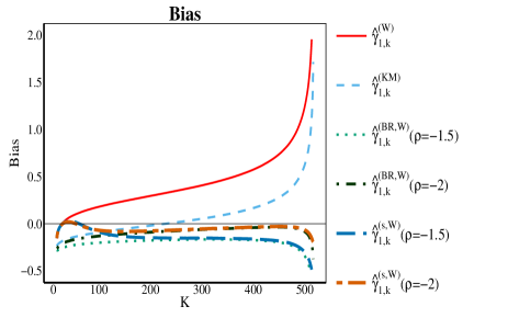
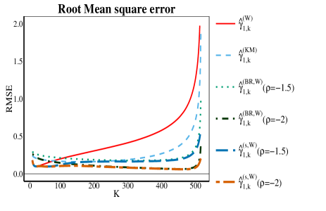
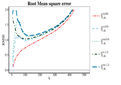
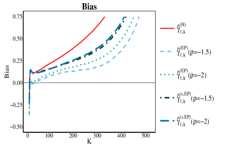
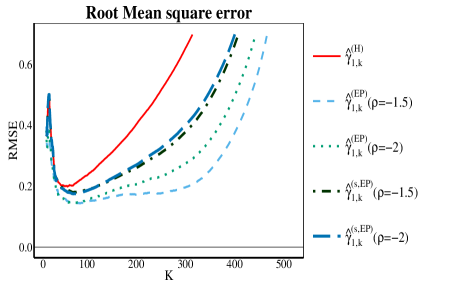
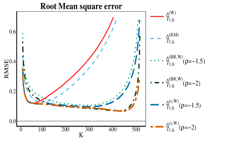
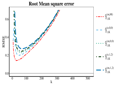
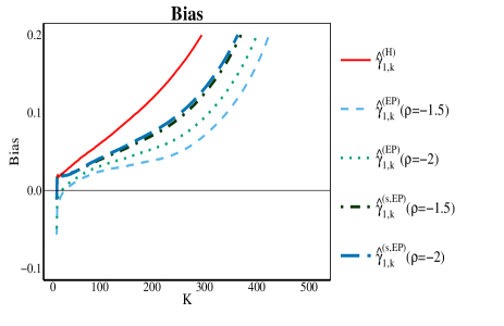
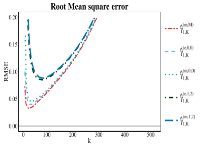
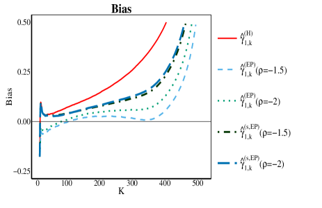
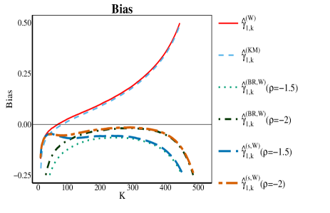
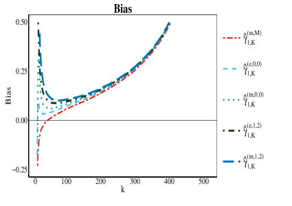
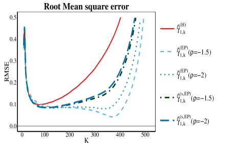
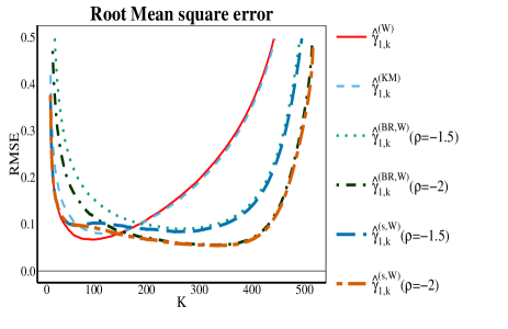
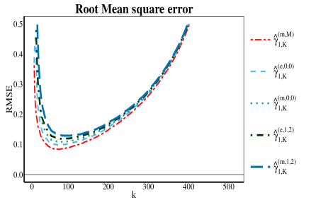
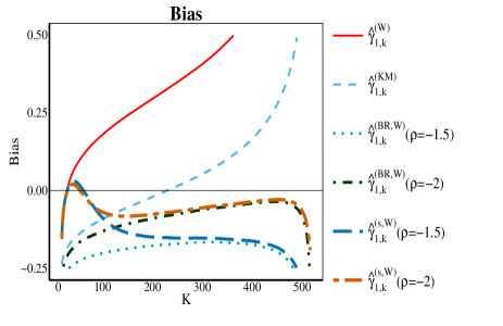
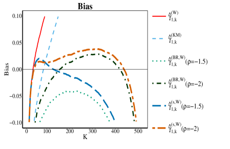
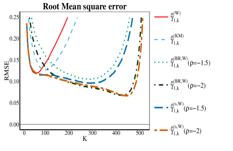
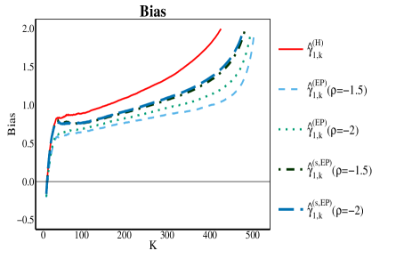
    Burr (10,2,2102210,2,2) censored by Burr (10,5,2105210,5,2) with Ξ³1=0.25subscript𝛾10.25\gamma_{1}=0.25 and Ξ³2=0.10subscript𝛾20.10\gamma_{2}=0.10, leading to heavy censoring with the proportion of non-censoring p=0.286𝑝0.286p=0.286; see Figure 1;

  • β€’

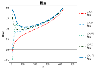
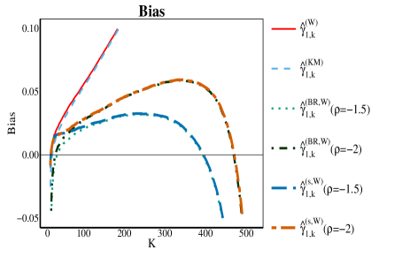
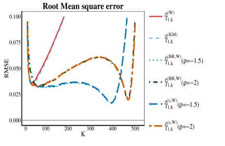
    Burr (10,2,1102110,2,1) censored by Burr (10,2,1102110,2,1) with Ξ³1=Ξ³2=0.5subscript𝛾1subscript𝛾20.5\gamma_{1}=\gamma_{2}=0.5 so that p=0.5𝑝0.5p=0.5; see Figure 2;

  • β€’

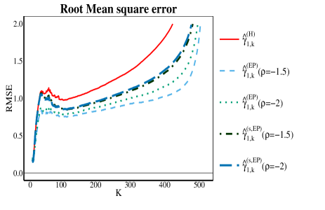
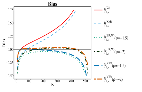
    Burr (10,5,2105210,5,2) censored by Burr (10,2,2102210,2,2) with Ξ³1=0.10subscript𝛾10.10\gamma_{1}=0.10 and Ξ³2=0.25subscript𝛾20.25\gamma_{2}=0.25, with light censoring p=0.714𝑝0.714p=0.714; see Figure 3;

  • β€’

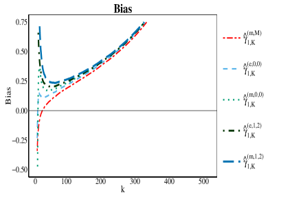
    FrΓ©chet (2) censored by FrΓ©chet (1) with Ξ³1=0.5subscript𝛾10.5\gamma_{1}=0.5 and Ξ³2=1subscript𝛾21\gamma_{2}=1, so that p=2/3𝑝23p=2/3; see Figure 4.

In each of these four cases we consider the results for

  • β€’

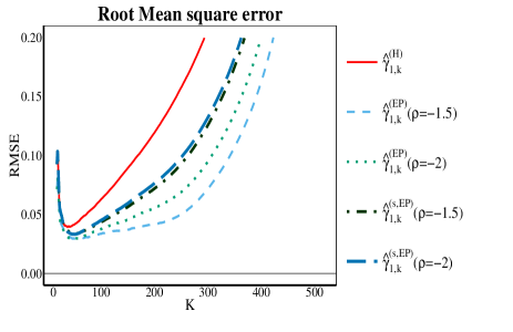
    Ξ³^1,k(H)superscriptsubscript^𝛾1π‘˜π»\hat{\gamma}_{1,k}^{(H)} from (2) , Ξ³^1,k(E​P)​(Οβˆ—)superscriptsubscript^𝛾1π‘˜πΈπ‘ƒsubscript𝜌\hat{\gamma}_{1,k}^{(EP)}(\rho_{*}) from (9), and Ξ³^1,k(s,E​P)​(Οβˆ—)superscriptsubscript^𝛾1π‘˜π‘ πΈπ‘ƒsubscript𝜌\hat{\gamma}_{1,k}^{(s,EP)}(\rho_{*}) from (16) with Ο‰=1πœ”1\omega=1 and for different values of Οβˆ—subscript𝜌\rho_{*} (left in Figures 1-4),

  • β€’

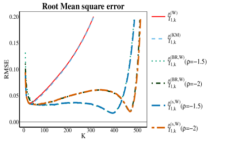
    Ξ³^1,k(W)superscriptsubscript^𝛾1π‘˜π‘Š\hat{\gamma}_{1,k}^{(W)} from (3), Ξ³^1,k(K​M)superscriptsubscript^𝛾1π‘˜πΎπ‘€\hat{\gamma}_{1,k}^{(KM)} from (4), Ξ³^1,k(B​R,W)​(ρ1)superscriptsubscript^𝛾1π‘˜π΅π‘…π‘Šsubscript𝜌1\hat{\gamma}_{1,k}^{(BR,W)}(\rho_{1}) from (14), and Ξ³^1,k(s,W)​(ρ1)superscriptsubscript^𝛾1π‘˜π‘ π‘Šsubscript𝜌1\hat{\gamma}_{1,k}^{(s,W)}(\rho_{1}) from (15) with Ο‰=1πœ”1\omega=1 and for different values of ρ1subscript𝜌1\rho_{1} (see middle of Figures 1-4),

  • β€’

    the Bayesian estimators Ξ³^1,k(m,M)superscriptsubscript^𝛾1π‘˜π‘šπ‘€\hat{\gamma}_{1,k}^{(m,M)}, Ξ³^1,k(e,1,2)superscriptsubscript^𝛾1π‘˜π‘’12\hat{\gamma}_{1,k}^{(e,1,2)} and Ξ³^1,k(m,1,2)superscriptsubscript^𝛾1π‘˜π‘š12\hat{\gamma}_{1,k}^{(m,1,2)} from (5), (6) and (7) (right in Figures 1-4).

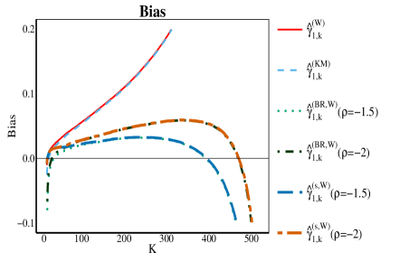
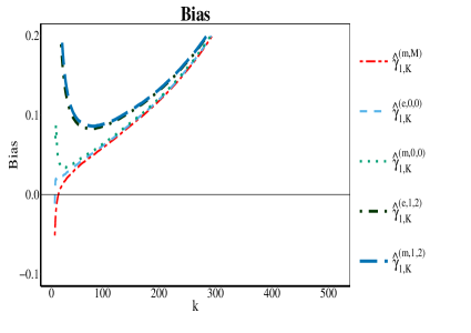
One observes that in case p<0.5𝑝0.5p<0.5 the likelihood based estimator Ξ³^1,k(H)superscriptsubscript^𝛾1π‘˜π»\hat{\gamma}_{1,k}^{(H)} and its bias reduced versions, and the Bayesian estimators have larger bias than the estimators derived from estimating the functional form Ltsubscript𝐿𝑑L_{t} in (1). Bias reduction of Ξ³^1,k(H)superscriptsubscript^𝛾1π‘˜π»\hat{\gamma}_{1,k}^{(H)} helps only partially in such cases. In these cases the bias reduced and penalized estimators Ξ³^1,k(B​R,W)superscriptsubscript^𝛾1π‘˜π΅π‘…π‘Š\hat{\gamma}_{1,k}^{(BR,W)} and Ξ³^1,k(s,W)​(ρ1)superscriptsubscript^𝛾1π‘˜π‘ π‘Šsubscript𝜌1\hat{\gamma}_{1,k}^{(s,W)}(\rho_{1}) perform good with low bias and low RMSE for a long interval of values of kπ‘˜k which is quite helpful in choosing an appropriate value of kπ‘˜k. This is in contrast with the bias of Ξ³^1,k(W)superscriptsubscript^𝛾1π‘˜π‘Š\hat{\gamma}_{1,k}^{(W)} and Ξ³^1,k(K​M)superscriptsubscript^𝛾1π‘˜πΎπ‘€\hat{\gamma}_{1,k}^{(KM)} which is systematically decreasing with decreasing value of kπ‘˜k. In order to evaluate the effect of the penalization in Ξ³^1,k(s,W)​(ρ1)superscriptsubscript^𝛾1π‘˜π‘ π‘Šsubscript𝜌1\hat{\gamma}_{1,k}^{(s,W)}(\rho_{1}), we focused the scale for the bias and RMSE plots in the Burr cases, see Figure 5. Especially in case p≀0.5𝑝0.5p\leq 0.5 and for smaller values of kπ‘˜k the mean of the shrinkage estimator is much more stable and ultimately for small kπ‘˜k the bahaviour of this estimator follows that of Ξ³^1,k(W)superscriptsubscript^𝛾1π‘˜π‘Š\hat{\gamma}_{1,k}^{(W)}. The resulting RMSE is then also a lower envelope of the RMSE curves of Ξ³^1,k(W)superscriptsubscript^𝛾1π‘˜π‘Š\hat{\gamma}_{1,k}^{(W)} and Ξ³^1,k(B​R,W)superscriptsubscript^𝛾1π‘˜π΅π‘…π‘Š\hat{\gamma}_{1,k}^{(BR,W)}.

On the other hand when p>0.5𝑝0.5p>0.5, and especially in the FrΓ©chet case, the basic estimators Ξ³^1,k(H)superscriptsubscript^𝛾1π‘˜π»\hat{\gamma}_{1,k}^{(H)}, Ξ³^1,k(W)superscriptsubscript^𝛾1π‘˜π‘Š\hat{\gamma}_{1,k}^{(W)} and Ξ³^1,k(m,M)superscriptsubscript^𝛾1π‘˜π‘šπ‘€\hat{\gamma}_{1,k}^{(m,M)} work almost equally well, and this also holds for the different approaches to bias reduction. Within the group of Bayes estimators clearly Ξ³^1,k(m,M)superscriptsubscript^𝛾1π‘˜π‘šπ‘€\hat{\gamma}_{1,k}^{(m,M)} works best.

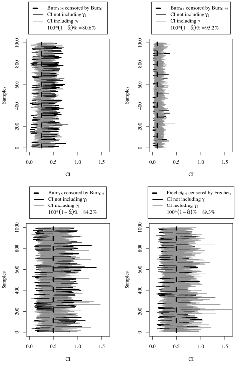
We also tested the proposed bootstrap procedure in the same cases as considered in Figures 1 to 4. We applied the algorithm with Ξ±=0.05𝛼0.05\alpha=0.05 and N=1000𝑁1000N=1000 to 1000 samples of size n=500𝑛500n=500. In Figure 6 the 1000 confidence intervals are given when choosing k^1subscript^π‘˜1\hat{k}_{1} and k^2subscript^π‘˜2\hat{k}_{2} adaptively using Ο΅=0.01italic-Ο΅0.01\epsilon=0.01, and when keeping k^1=k^2subscript^π‘˜1subscript^π‘˜2\hat{k}_{1}=\hat{k}_{2} fixed to 25=0.05Γ—n250.05𝑛25=0.05\times n throughout (this value of kπ‘˜k appears appropriate on the basis of Figures 1 to 4). Further simulations showed that for n=1000𝑛1000n=1000 keeping k^1=k^2subscript^π‘˜1subscript^π‘˜2\hat{k}_{1}=\hat{k}_{2} fixed to 0.04Γ—n0.04𝑛0.04\times n leads to confidence intervals that attain the required 95% level closely. The confidence intervals missing the correct value of Ξ³1subscript𝛾1\gamma_{1} are put in dark grey. Of course when the kπ‘˜k values are chosen adaptively, it is more difficult to attain the confidence level 1βˆ’Ξ±=0.951𝛼0.951-\alpha=0.95.

A deeper understanding of the distribution of Ξ³^1,k(W)superscriptsubscript^𝛾1π‘˜π‘Š\hat{\gamma}_{1,k}^{(W)} and E^k​(βˆ’Ξ²1)subscript^πΈπ‘˜subscript𝛽1\hat{E}_{k}(-\beta_{1}) appears necessary to enhance the adaptive choice of k1,k2subscriptπ‘˜1subscriptπ‘˜2k_{1},k_{2} and the performance of the bootstrap algorithm.

6 A case study from car insurance

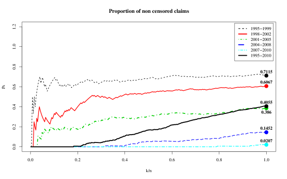
Finally, in order to illustrate the merits of the newly proposed method, we consider a data set with indexed total payments from a motor third party liability insurance company operating in the EU, with records from 1995 till 2010 with n=849𝑛849n=849 claims of which only 340 were completely developed at the end of 2010. For every claim the indexed cumulative payments are given at the end of every year until development. In Figure 6 we plotted the proportions of non-censored data p^ksubscript^π‘π‘˜\hat{p}_{k} which are situated in the top 100​k/n100π‘˜π‘›100k/n% of cumulative payments at the end of 2010 as a function of k/nπ‘˜π‘›k/n. In practice most companies substitute the censored observations by ultimate predictions obtained through reserving techniques. Here we show how the extreme value methods for censored data can also be used directly without ultimates in order to obtain relevant extreme value predictions.

Due to the long-tail nature of such portfolios, only the claims with arrival year between 1995 and 1999 can be considered to satisfy the condition of weak censoring p>0.5𝑝0.5p>0.5 or Ξ³1<Ξ³2subscript𝛾1subscript𝛾2\gamma_{1}<\gamma_{2} when using the information up to 2010. For this group of early claims 29% is censored at the end of 2010, while the percentage of censoring is 60% when considering all claims. Note also that when considering all claims the largest 20 % are all censored, whereas this amount increases to 40% for the claims arriving after 2003. Needless to say that extreme value methodology is quite challenging in such a case.

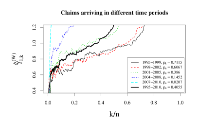
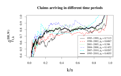
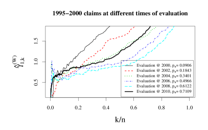
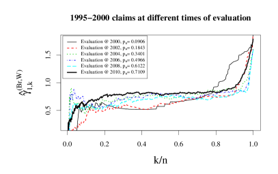
In order to illustrate the stability of the proposed bias reduction technique based on the Worms and Worms estimator over different percentages of censoring, we also split the full data set in groups along the arrival times in 1995-1999, 1998-2002, 2001-2005, 2004-2008, 2007-2010. In Figure 7 the original estimates Ξ³^1,k(W)superscriptsubscript^𝛾1π‘˜π‘Š\hat{\gamma}_{1,k}^{(W)} and Ξ³^1,k(B​R,W)​(βˆ’3)superscriptsubscript^𝛾1π‘˜π΅π‘…π‘Š3\hat{\gamma}_{1,k}^{(BR,W)}(-3) are given as a function of k/nπ‘˜π‘›k/n for each of these subgroups and for the complete data set. The value ρ1=βˆ’3subscript𝜌13\rho_{1}=-3 was chosen as this value yields the most constant plots as a function of kπ‘˜k. The plots of Ξ³^1,k(W)superscriptsubscript^𝛾1π‘˜π‘Š\hat{\gamma}_{1,k}^{(W)} are steepest for the claims which are most recent in 2010. The stability of the bias reduced estimates over these subgroups is quite convincing leading to estimates of Ξ³1subscript𝛾1\gamma_{1} between 0.6 and 0.7.

As another validity check, in Figure 8 we consider only the claims from 1995-1999 with their cumulative payments as of 2000 till 2010 in steps of 2 years. Note that in 2000 only 9% of those claims were fully developed, while at 2010 this percentage rose to 71%. Again the bias reduced estimates Ξ³^1,k(B​R,W)​(βˆ’3)superscriptsubscript^𝛾1π‘˜π΅π‘…π‘Š3\hat{\gamma}_{1,k}^{(BR,W)}(-3) are remarkably stable over kπ‘˜k.

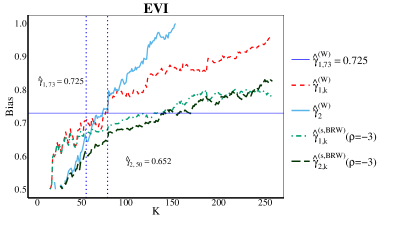
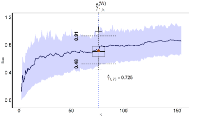
We also applied the bootstrap algorithm to this case study. Using Ο΅=0.01italic-Ο΅0.01\epsilon=0.01 leads to k^1=73subscript^π‘˜173\hat{k}_{1}=73, k^2=50subscript^π‘˜250\hat{k}_{2}=50, Ξ³^1,73(W)=0.725superscriptsubscript^𝛾173π‘Š0.725\hat{\gamma}_{1,73}^{(W)}=0.725, and Ξ³^2,50(W)=0.652superscriptsubscript^𝛾250π‘Š0.652\hat{\gamma}_{2,50}^{(W)}=0.652, see Figure 10 (left). The confidence intervals for the different values of kπ‘˜k are given in Figure 10 (right) with special attention for the case k=73π‘˜73k=73 which leads to the interval 95% confidence interval (0.48;0.91)0.480.91(0.48;0.91). Choosing k^1=k^2subscript^π‘˜1subscript^π‘˜2\hat{k}_{1}=\hat{k}_{2} fixed at 4 to 5% of the sample size n=849𝑛849n=849, as suggested in the simulation section, leads to lower bounds that are somewhat lower than 0.48, as can be seen from Figure 10 (right).

7 Conclusion

The estimator Ξ³^1,k(W)superscriptsubscript^𝛾1π‘˜π‘Š\hat{\gamma}_{1,k}^{(W)} from Worms and Worms (2014) has the best RMSE behaviour between all available first order estimators of Ξ³1subscript𝛾1\gamma_{1}. In order to enhance the practical use of this estimator we proposed bias reduction and penalization techniques which lead to improved bias and RMSE behaviour. Moreover a bootstrap procedure is proposed in order to construct confidence intervals. This is especially useful with long-tailed insurance products. In order to enhance the adaptive choice of the number of extreme data kπ‘˜k asymptotic representations of the estimators involved are needed for all cases, but especially in case of heavy censoring. This will be the subject of future work.

8 Acknowledgments

The authors are indebted to Rym and Julien Worms for helpful discussions and suggestions on this topic. This work is based on the research supported wholly/in part by the National Research Foundation of South Africa (Grant Number 102628). The Grantholder acknowledges that opinions, findings and conclusions or recommendations expressed in any publication generated by the NRF supported research is that of the author(s), and that the NRF accepts no liability whatsoever in this regard.

References

  • [1] Ameraoui, A., Boukhetala, K. and Dupuy, J.-F., 2016. Bayesian estimation of the tail index of a heavy tailed distribution under random censoring. Computational Statistics and Data Analysis, 104, 148-168
  • [2] Beirlant, J., Bardoutsos, A., de Wet, T. and Gijbels, I., 2016. Bias reduced tail estimation for censored Pareto type distribution. Statistics and Probability Letters 109, 78-88.
  • [3] Beirlant, J., Guillou, A., Dierckx, G. and Fils-Villetard, A., 2007. Estimation of the extreme value index and extreme quantiles under random censoring. Extremes 10, 151-174.
  • [4] Beirlant, J., Joossens, E. and Segers, J., 2009. Second-order refined peaks-over-threshold modelling for heavy-tailed distributions. Journal of Statistical Planning and Inference 139, 2800-2815.
  • [5] Beirlant, J., Maribe, G. and Verster, A., 2017. Using shrinkage estimators to reduce bias and MSE in estimation of heavy tails. To appear in Revstat.
  • [6] Brahimi, B., Meraghni, D. and Necir, A., 2015. Approximations to the tail index estimator of a heavy-tailed distribution under random censoring and application. Math. Methods. Statist. 24, 266-279.
  • [7] Brahimi, B., Meraghni, D. and Necir, A., 2016. Nelson-Aalen tail product-limit estimation under random censorship. arXiv:1502.03955v2
  • [8] Einmahl, J., Fils-Villetard, A. and Guillou, A., 2008. Statistics of extremes under random censoring. Bernoulli 14, 2007-227.
  • [9] Fraga Alves, M.I., Gomes, M.I. and de Haan, L., 2003. A new class of semi-parametric estimators of the second order parameter. Portugaliae Mathematica 60, 193-214.
  • [10] Gomes, M.I. and Neves, M.M., 2011. Estimation of the extreme value index for randomly censored data. Biometrical Letters, 48, 1-22.
  • [11] Gomes, M.I. and Oliveira, O., 2003. Censoring estimators of a positive tail index. Statistics and Probability Letters, 65, 147-159.
  • [12] Hill, B.M., 1975. A simple general approach about the tail of a distribution. Annals of Statistics 3, 1163-1174.
  • [13] Worms, J. and Worms, R., 2014. New estimators of the extreme value index under random right censoring for heavy-tailed distributions. Extremes 17, 337-358.
  • [14] Worms, J. and Worms, R., 2017. Extreme value statistics for censored data with heavy tail under competing risks. ExtremesCompetingRisks-HAL-13jan17.pdf
  • [15] Zellner, A., 1971. An Introduction to Bayesian Inference in Econometrics. Wiley.
Refer to caption
Refer to caption
Refer to caption
Refer to caption
Refer to caption
Refer to caption
Figure 1: Bias and RMSE for Burr(10,2,2) censored by Burr(10,5,2)
Refer to caption
Refer to caption
Refer to caption
Refer to caption
Refer to caption
Refer to caption
Figure 2: Bias and RMSE for Burr(10,2,1) censored by Burr(10,2,1)
Refer to caption
Refer to caption
Refer to caption
Refer to caption
Refer to caption
Refer to caption
Figure 3: Bias and RMSE for Burr(10,5,2) censored by Burr(10,2,2)
Refer to caption
Refer to caption
Refer to caption
Refer to caption
Refer to caption
Refer to caption
Figure 4: Bias and RMSE for FrΓ©chet(2) censored by FrΓ©chet(1)
Refer to caption
Refer to caption
Refer to caption
Refer to caption
Refer to caption
Refer to caption
Figure 5: Bias (top) and RMSE (bottom) for Ξ³^1,k(W)superscriptsubscript^𝛾1π‘˜π‘Š\hat{\gamma}_{1,k}^{(W)}, Ξ³^1,k(B​R,W)​(βˆ’1.5)superscriptsubscript^𝛾1π‘˜π΅π‘…π‘Š1.5\hat{\gamma}_{1,k}^{(BR,W)}(-1.5), Ξ³^1,k(B​R,W)​(βˆ’2)superscriptsubscript^𝛾1π‘˜π΅π‘…π‘Š2\hat{\gamma}_{1,k}^{(BR,W)}(-2), Ξ³^1,k(s,W)​(βˆ’1.5)superscriptsubscript^𝛾1π‘˜π‘ π‘Š1.5\hat{\gamma}_{1,k}^{(s,W)}(-1.5), Ξ³^1,k(s,W)​(βˆ’2)superscriptsubscript^𝛾1π‘˜π‘ π‘Š2\hat{\gamma}_{1,k}^{(s,W)}(-2) in case of Burr(10,2,2) censored by Burr(10,5,2) (left); Burr(10,2,1) censored by Burr(10,2,1) (middle); and Burr(10,5,2) censored by Burr(10,2,2) (right)
Refer to caption
Refer to caption
Figure 6: Simulated bootstrap 95% confidence intervals with adaptive choice of k1subscriptπ‘˜1k_{1} and k2subscriptπ‘˜2k_{2} using Ο΅=0.01italic-Ο΅0.01\epsilon=0.01 (4 left frames) and using k1=k2=25=5%​nsubscriptπ‘˜1subscriptπ‘˜225percent5𝑛k_{1}=k_{2}=25=5\%n for every sample (4 right frames)
Refer to caption
Figure 7: Car liability data: plot of p^ksubscript^π‘π‘˜\hat{p}_{k} as a function of k/nπ‘˜π‘›k/n for all claims jointly (thick full line) and for claims that arrived in different time intervals.
Refer to caption
Refer to caption
Figure 8: Car liability data: Ξ³^1,k(W)superscriptsubscript^𝛾1π‘˜π‘Š\hat{\gamma}_{1,k}^{(W)} (left) and Ξ³^1,k(B​R,W)​(βˆ’3)superscriptsubscript^𝛾1π‘˜π΅π‘…π‘Š3\hat{\gamma}_{1,k}^{(BR,W)}(-3) (right) based on indexed cumulative payments at end of 2010, as a function of k/nπ‘˜π‘›k/n for all claims together (thick full line) and for claims arriving in different time periods
Refer to caption
Refer to caption
Figure 9: Car liability data: Ξ³^1,k(W)superscriptsubscript^𝛾1π‘˜π‘Š\hat{\gamma}_{1,k}^{(W)} (left) and Ξ³^1,k(B​R,W)​(βˆ’3)superscriptsubscript^𝛾1π‘˜π΅π‘…π‘Š3\hat{\gamma}_{1,k}^{(BR,W)}(-3) (right) for all claims arriving in 1995-1999 and based on indexed cumulative payments at end of 2000(02)2010, as a function of k/nπ‘˜π‘›k/n.
Refer to caption
Refer to caption
Figure 10: Car liability data, using all claims: Ξ³^1,k(W)superscriptsubscript^𝛾1π‘˜π‘Š\hat{\gamma}_{1,k}^{(W)}, Ξ³^1,k(s,W)​(βˆ’3)superscriptsubscript^𝛾1π‘˜π‘ π‘Š3\hat{\gamma}_{1,k}^{(s,W)}(-3), Ξ³^2,k(W)superscriptsubscript^𝛾2π‘˜π‘Š\hat{\gamma}_{2,k}^{(W)}, Ξ³^2,k(s,W)​(βˆ’3)superscriptsubscript^𝛾2π‘˜π‘ π‘Š3\hat{\gamma}_{2,k}^{(s,W)}(-3) (left); 95% bootstrap confidence intervals (right).