Analysis of the effectiveness of the truth-spreading strategy for inhibiting rumors

Lu-Xing Yang ylx910920@gmail.com Pengdeng Li 1414797521@qq.com Xiaofan Yang xfyang1964@gmail.com Yingbo Wu wyb@cqu.edu.cn Yuan Yan Tang yytang@umac.mo Faculty of Electrical Engineering, Mathematics and Computer Science, Delft University of Technology, Delft, GA 2600, The Netherlands School of Software Engineering, Chongqing University, Chongqing, 400044, China Department of Computer and Infomation Science, The University of Macau, Macau
Abstract

Spreading truths is recognized as a feasible strategy for inhibiting rumors. This paper is devoted to assessing the effectiveness of the truth-spreading strategy. An individual-level rumor-truth spreading model (the generic URTU model) is derived. Under the model, two criteria for the termination of a rumor are presented. These criteria capture the influence of the network structures on the effectiveness of the truth-spreading strategy. Extensive simulations show that, when the rumor or the truth terminates, the dynamics of a simplified URTU model (the linear URTU model) fits well with the actual rumor-truth interplay process. Therefore, the generic URTU model forms a theoretical basis for assessing the effectiveness of the truth-spreading strategy for restraining rumors.

keywords:
rumor/truth spreading , rumor/truth spreading network , generic/linear rumor-truth spreading model , spectral radius
โ€ โ€ journal: Nonlinear Analysis: Real World Applications

1 Introduction

Rumors are loosely defined as unconfirmed elaborations or annotations of public things, events or issues. As an important form of social interactions, rumor spreading has a significant impact on human affairs. The rapidly popularized online social networks (OSNs) offer a shortcut for the fast spread of rumors, greatly enlarging their influence [1, 2, 3]. Unfortunately, most rumors could induce social panic or economic loss [4]. For example, Syrian hackers once broke into the twitter account of Associated Press (AP) and dispersed the rumor that explosions at White House had injured Obama, leading to 10 billion USD losses before the rumor was clarified [5]. Therefore, one of the major concerns in the field of cybersecurity is to contain the prevalence of rumors in OSNs [6].

The rumor spreading dynamics is intended to model and study the spreading process of rumors, so as to gain insight into the influence of different factors on the prevalence of rumors and thereby to work out cost-effective strategies of restraining rumors. In 1964, Daley and Kendall [7] introduced the first rumor spreading model (the DK model) by modeling the spreading process of rumors as a discrete-time iterative process on fully connected networks. Later, Maki and Thompson [8] advised a variant of the DK model (the MT model). In his PhD thesis, Cintron-Arias [9] suggested a differential dynamical system model capturing the spread of rumors by introducing the state transition rates to the DK model. Since then, a multitude of rumor spreading models on homogeneous networks have been proposed, aiming at understanding the influence of different factors, such as the memory [10, 11], the skepticism and denial [12], the incubation [13, 14], the education or scientific knowledge [15, 16], the latency [17], the government behavior [18] and others [19], on the prevalence of rumors.

A series of emperical studies starting at the end of last century show that, surprisingly, OSNs are heterogeneous rather than homogeneous [20, 21]. From then on, much effort has been put to inspect the spread of rumors on complex networks with the aid of the mean-field theory, with emphasis on the influence of different factors such as the network heterogeneity [22], the nonlinear spreading rate [23], the incubation [24], the memory [25, 26], the trust between individuals [27], the countermeasures [28, 29, 30], the latency [31, 32], the time-varying parameters [33], the government punishment [34], the heterogeneous transmission [35] and others [36, 37]. As these models are quite rough, their dynamics may severely deviate from the actual rumor spreading process. Furthermore, the genuine influence of the network topology on the rumor spreading cannot be made certain by studying these models.

In 2009, Van Mieghem et al. [38] proposed a (continuous-time) individual-level epidemic model (the exact SIS model), which accurately captures the average dynamics of the SIS epidemic [38, 39]. In pursuit of this idea, a number of individual-level epidemic models have recently been reported [40, 41, 42, 43, 44, 45, 46]. Continuous-time individual-level models are especially efficacious in exploring the impact of the network topology on the epidemic process and, hence, are suited to the study of rumor spreading. To our knowledge, so far there is no report in this aspect.

Clarifying rumors by spreading truths is a feasible strategy for inhibiting rumors in OSNs [47, 48]. Before the appearance of a rumor and the truth, all persons in the OSN are uncertain. After the appearance of the rumor and the truth, depending on personal judgement or/and knowledge, a person either believes the rumor, or believes the truth, or is uncertain (i.e., believe neither the rumor nor the truth). This paper is devoted to assessing the effectiveness of the truth-spreading strategy. An individual-level rumor-truth spreading model (the generic URTU model) is derived. Then two criteria for the extinction of a rumor are presented, which capture the influence of the network structures on the effectiveness of the truth-spreading strategy. Extensive simulations show that, when the rumor or the truth tends to extinction, the dynamics of a simplified URTU model (the linear URTU model) fits well with the actual rumor-truth interplay process. Therefore, the generic URTU model provides a proper basis for assessing the effectiveness of the truth-spreading strategy for restraining rumors.

The subsequent materials are organized in this fashion. Section 2 derives the generic URTU model as well as the linear URTU model. Section 3 studies the dynamics of the generic URTU model. Experimental results examining the effectiveness of the linear URTU model are reported in Section 4. Finally, Section 5 summarizes this work.

2 A generic rumor-truth spreading model

This section is dedicated to establishing a generic continuous-time dynamic model capturing the interaction between a rumor and the truth.

2.1 Notions, notations and hypotheses

Suppose a rumor and the truth spread in an OSN consisting of N๐‘N persons labelled 1,2,โ€ฆ,N12โ€ฆ๐‘1,2,...,N. Let V={1,2,โ‹ฏ,N}๐‘‰12โ‹ฏ๐‘V=\{1,2,\cdots,N\}. Suppose the rumor is propagated through a rumor-spreading network GR=(V,ER)subscript๐บ๐‘…๐‘‰subscript๐ธ๐‘…G_{R}=(V,E_{R}), where (i,j)โˆˆER๐‘–๐‘—subscript๐ธ๐‘…(i,j)\in E_{R} if and only if person j๐‘—j can tell the rumor to person i๐‘–i. Suppose the truth is circulated through a truth-spreading network GT=(V,ET)subscript๐บ๐‘‡๐‘‰subscript๐ธ๐‘‡G_{T}=(V,E_{T}), where (i,j)โˆˆET๐‘–๐‘—subscript๐ธ๐‘‡(i,j)\in E_{T} if and only if person j๐‘—j can tell the truth to person i๐‘–i. In what follows, the two networks are always assumed to be strongly connected.

At the beginning, there is neither the rumor nor the truth, so all persons in the OSN are uncertain. After the appearance of the rumor and the truth, every person in the OSN is assumed to be in one of three possible states: rumor-believing, truth-believing, and uncertain. A rumor-believing person believes the rumor, a truth-believing person believes the truth, and an uncertain person believes neither the rumor nor the truth. Depending on personal judgement on the event, every person may choose to believe the rumor, or to believe the truth, or to be uncertain. Let Xiโ€‹(t)subscript๐‘‹๐‘–๐‘กX_{i}(t) = 0, 1, and 2 denote that, at time t๐‘กt, person i๐‘–i is uncertain, rumor-believing, and truth-believing, respectively. Then the state of the OSN at time t๐‘กt is represented by the vector

๐—โ€‹(t)=(X1โ€‹(t),X2โ€‹(t),โ‹ฏ,XNโ€‹(t))T.๐—๐‘กsuperscriptsubscript๐‘‹1๐‘กsubscript๐‘‹2๐‘กโ‹ฏsubscript๐‘‹๐‘๐‘ก๐‘‡\mathbf{X}(t)=(X_{1}(t),X_{2}(t),\cdots,X_{N}(t))^{T}.

Next, let us introduce a set of hypotheses as follows.

  1. (H1)

    Due to the influence of a rumor-believer j๐‘—j, at any time an uncertain person i๐‘–i turns to believe the rumor at rate ฮฒiโ€‹jUโ‰ฅ0superscriptsubscript๐›ฝ๐‘–๐‘—๐‘ˆ0\beta_{ij}^{U}\geq 0. Here, ฮฒiโ€‹jU>0superscriptsubscript๐›ฝ๐‘–๐‘—๐‘ˆ0\beta_{ij}^{U}>0 if and only if (i,j)โˆˆER๐‘–๐‘—subscript๐ธ๐‘…(i,j)\in E_{R}. ฮฒiโ€‹jUsuperscriptsubscript๐›ฝ๐‘–๐‘—๐‘ˆ\beta_{ij}^{U} is proportional to (a) the rate at which person j๐‘—j tells the rumor to person i๐‘–i, and (b) the probability of person i๐‘–i believing the rumor when hearing it. Let ๐U=(ฮฒiโ€‹jU)Nร—Nsubscript๐๐‘ˆsubscriptsuperscriptsubscript๐›ฝ๐‘–๐‘—๐‘ˆ๐‘๐‘\mathbf{B}_{U}=\left(\beta_{ij}^{U}\right)_{N\times N}. This hypothesis captures the influence of the rumor spreading on uncertain persons.

  2. (H2)

    Due to the influence of a rumor-believer j๐‘—j, at any time a truth-believer i๐‘–i turns to believe the rumor at rate ฮฒiโ€‹jTโ‰ฅ0superscriptsubscript๐›ฝ๐‘–๐‘—๐‘‡0\beta_{ij}^{T}\geq 0. Here, ฮฒiโ€‹jT>0superscriptsubscript๐›ฝ๐‘–๐‘—๐‘‡0\beta_{ij}^{T}>0 if and only if (i,j)โˆˆER๐‘–๐‘—subscript๐ธ๐‘…(i,j)\in E_{R}. ฮฒiโ€‹jTsuperscriptsubscript๐›ฝ๐‘–๐‘—๐‘‡\beta_{ij}^{T} is proportional to (a) the rate at which person j๐‘—j tells the rumor to person i๐‘–i, and (b) the probability of person i๐‘–i believing the rumor when hearing it. Let ๐T=(ฮฒiโ€‹jT)Nร—Nsubscript๐๐‘‡subscriptsuperscriptsubscript๐›ฝ๐‘–๐‘—๐‘‡๐‘๐‘\mathbf{B}_{T}=\left(\beta_{ij}^{T}\right)_{N\times N}. This hypothesis captures the influence of the rumor spreading on truth-believers. Certainly, we have ฮฒiโ€‹jTโ‰คฮฒiโ€‹jUsuperscriptsubscript๐›ฝ๐‘–๐‘—๐‘‡superscriptsubscript๐›ฝ๐‘–๐‘—๐‘ˆ\beta_{ij}^{T}\leq\beta_{ij}^{U}.

  3. (H3)

    Due to the influence of a truth-believer j๐‘—j, at any time an uncertain person i๐‘–i turns to believe the truth at rate ฮณiโ€‹jUโ‰ฅ0superscriptsubscript๐›พ๐‘–๐‘—๐‘ˆ0\gamma_{ij}^{U}\geq 0, Here, ฮณiโ€‹jU>0superscriptsubscript๐›พ๐‘–๐‘—๐‘ˆ0\gamma_{ij}^{U}>0 if and only if (i,j)โˆˆET๐‘–๐‘—subscript๐ธ๐‘‡(i,j)\in E_{T}. ฮณiโ€‹jUsuperscriptsubscript๐›พ๐‘–๐‘—๐‘ˆ\gamma_{ij}^{U} is proportional to (a) the rate at which person j๐‘—j tells the truth to person i๐‘–i, and (b) the probability of person i๐‘–i believing the truth when hearing it. Let ๐‚U=(ฮณiโ€‹jU)Nร—Nsubscript๐‚๐‘ˆsubscriptsuperscriptsubscript๐›พ๐‘–๐‘—๐‘ˆ๐‘๐‘\mathbf{C}_{U}=\left(\gamma_{ij}^{U}\right)_{N\times N}. This hypothesis captures the influence of the truth spreading on uncertain persons.

  4. (H4)

    Due to the influence of a truth-believer j๐‘—j, at any time a rumor-believer i๐‘–i turns to believe the truth at rate ฮณiโ€‹jRโ‰ฅ0superscriptsubscript๐›พ๐‘–๐‘—๐‘…0\gamma_{ij}^{R}\geq 0, Here, ฮณiโ€‹jR>0superscriptsubscript๐›พ๐‘–๐‘—๐‘…0\gamma_{ij}^{R}>0 if and only if (i,j)โˆˆET๐‘–๐‘—subscript๐ธ๐‘‡(i,j)\in E_{T}. ฮณiโ€‹jRsuperscriptsubscript๐›พ๐‘–๐‘—๐‘…\gamma_{ij}^{R} is proportional to (a) the rate at which person j๐‘—j tells the truth to person i๐‘–i, and (b) the probability of person i๐‘–i believing the truth when hearing it. Let ๐‚R=(ฮณiโ€‹jR)Nร—Nsubscript๐‚๐‘…subscriptsuperscriptsubscript๐›พ๐‘–๐‘—๐‘…๐‘๐‘\mathbf{C}_{R}=\left(\gamma_{ij}^{R}\right)_{N\times N}. This hypothesis captures the influence of the truth spreading on rumor-believers. Certainly, we have ฮณiโ€‹jRโ‰คฮณiโ€‹jUsuperscriptsubscript๐›พ๐‘–๐‘—๐‘…superscriptsubscript๐›พ๐‘–๐‘—๐‘ˆ\gamma_{ij}^{R}\leq\gamma_{ij}^{U}.

  5. (H5)

    Due to the forgetfulness or the loss of interest, a rumor-believer i๐‘–i turns to be uncertain at rate ฮดiR>0superscriptsubscript๐›ฟ๐‘–๐‘…0\delta_{i}^{R}>0. Let ๐ƒR=dโ€‹iโ€‹aโ€‹gโ€‹(ฮดiR)subscript๐ƒ๐‘…๐‘‘๐‘–๐‘Ž๐‘”superscriptsubscript๐›ฟ๐‘–๐‘…\mathbf{D}_{R}=diag\left(\delta_{i}^{R}\right).

  6. (H6)

    Due to the forgetfulness or the loss of interest, a truth-believer i๐‘–i turns to be uncertain at rate ฮดiT>0superscriptsubscript๐›ฟ๐‘–๐‘‡0\delta_{i}^{T}>0. Let ๐ƒT=dโ€‹iโ€‹aโ€‹gโ€‹(ฮดiT)subscript๐ƒ๐‘‡๐‘‘๐‘–๐‘Ž๐‘”superscriptsubscript๐›ฟ๐‘–๐‘‡\mathbf{D}_{T}=diag\left(\delta_{i}^{T}\right).

All the forthcoming rumor-truth spreading models are assumed to comply with these hypotheses.

2.2 The original URTU model

For fundamental knowledge on continuous-time Markov chain, see Ref. [49].

Another way of representing the group state at time t๐‘กt is by the decimal number iโ€‹(t)=โˆ‘k=1NXkโ€‹(t)โ€‹3kโˆ’1๐‘–๐‘กsuperscriptsubscript๐‘˜1๐‘subscript๐‘‹๐‘˜๐‘กsuperscript3๐‘˜1i(t)=\sum_{k=1}^{N}X_{k}(t)3^{k-1}. In this context, there are totally 3Nsuperscript3๐‘3^{N} possible OSN states: 0,1,โ‹ฏ,3Nโˆ’101โ‹ฏsuperscript3๐‘10,1,\cdots,3^{N}-1. According to the previous hypotheses, the infinitesimal generator ๐=[qiโ€‹j]3Nร—3N๐subscriptdelimited-[]subscript๐‘ž๐‘–๐‘—superscript3๐‘superscript3๐‘\mathbf{Q}=\left[q_{ij}\right]_{3^{N}\times 3^{N}} for the rumor-truth spreading process is given as

qiโ€‹j={ฮดmRifi=j+3mโˆ’1;m=1,2,โ‹ฏ,N,xm=1ฮดmTifi=j+2โ‹…3mโˆ’1;m=1,2,โ‹ฏ,N,xm=2โˆ‘k=1Nฮฒmโ€‹kUโ€‹1{xk=1}ifi=jโˆ’3mโˆ’1;m=1,2,โ‹ฏ,N,xm=0โˆ‘k=1Nฮฒmโ€‹kTโ€‹1{xk=1}ifi=j+3mโˆ’1;m=1,2,โ‹ฏ,N,xm=2โˆ‘k=1Nฮณmโ€‹kUโ€‹1{xk=2}ifi=jโˆ’2โ‹…3mโˆ’1;m=1,2,โ‹ฏ,N,xm=0โˆ‘k=1Nฮณmโ€‹kRโ€‹1{xk=2}ifi=jโˆ’3mโˆ’1;m=1,2,โ‹ฏ,N,xm=1โˆ’โˆ‘k=0,kโ‰ iNโˆ’1qiโ€‹kifi=j0otherwise.q_{ij}=\left\{\begin{aligned} &\delta_{m}^{R}&\text{if}&\quad i=j+3^{m-1};\\ &&&\quad m=1,2,\cdots,N,x_{m}=1\\ &\delta_{m}^{T}&\text{if}&\quad i=j+2\cdot 3^{m-1};\\ &&&\quad m=1,2,\cdots,N,x_{m}=2\\ &\sum_{k=1}^{N}\beta_{mk}^{U}1_{\{x_{k}=1\}}&\text{if}&\quad i=j-3^{m-1};\\ &&&\quad m=1,2,\cdots,N,x_{m}=0\\ &\sum_{k=1}^{N}\beta_{mk}^{T}1_{\{x_{k}=1\}}&\text{if}&\quad i=j+3^{m-1};\\ &&&\quad m=1,2,\cdots,N,x_{m}=2\\ &\sum_{k=1}^{N}\gamma_{mk}^{U}1_{\{x_{k}=2\}}&\text{if}&\quad i=j-2\cdot 3^{m-1};\\ &&&\quad m=1,2,\cdots,N,x_{m}=0\\ &\sum_{k=1}^{N}\gamma_{mk}^{R}1_{\{x_{k}=2\}}&\text{if}&\quad i=j-3^{m-1};\\ &&&\quad m=1,2,\cdots,N,x_{m}=1\\ &-\sum_{k=0,k\neq i}^{N-1}q_{ik}&\text{if}&\quad i=j\\ &0\quad&\quad&\text{otherwise}.\end{aligned}\right. (1)

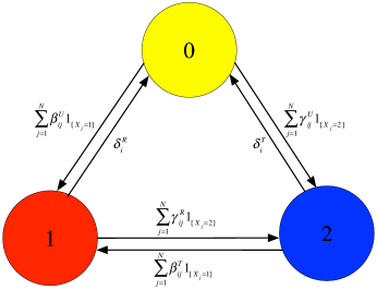
where i=โˆ‘k=1Nxkโ€‹3kโˆ’1๐‘–superscriptsubscript๐‘˜1๐‘subscript๐‘ฅ๐‘˜superscript3๐‘˜1i=\sum_{k=1}^{N}x_{k}3^{k-1}, 1Asubscript1๐ด1_{A} stands for the indicator function of set A๐ดA. The continuous-time Markov chain model with the infinitesimal generator ๐๐\mathbf{Q} is referred to as the original Uncertain-Rumor-Truth-Uncertain (URTU) model. See Fig. 1 for the state transition rates of a person under the original URTU model.
Refer to caption
Figure 1: The state transition rates of person i๐‘–i under the original URTU model.

2.3 The exact URTU model

Let siโ€‹(t)subscript๐‘ ๐‘–๐‘กs_{i}(t) denote the probability that the group state at time t๐‘กt is i=โˆ‘k=1Nxkโ€‹3kโˆ’1๐‘–superscriptsubscript๐‘˜1๐‘subscript๐‘ฅ๐‘˜superscript3๐‘˜1i=\sum_{k=1}^{N}x_{k}3^{k-1}. That is,

siโ€‹(t)=Prโก{X1โ€‹(t)=x1,โ‹ฏ,XNโ€‹(t)=xN}.subscript๐‘ ๐‘–๐‘กPrsubscript๐‘‹1๐‘กsubscript๐‘ฅ1โ‹ฏsubscript๐‘‹๐‘๐‘กsubscript๐‘ฅ๐‘s_{i}(t)=\Pr\left\{X_{1}(t)=x_{1},\cdots,X_{N}(t)=x_{N}\right\}.

Let ๐ฌโ€‹(t)=[s0โ€‹(t),โ‹ฏ,s3Nโˆ’1โ€‹(t)]T๐ฌ๐‘กsuperscriptsubscript๐‘ 0๐‘กโ‹ฏsubscript๐‘ superscript3๐‘1๐‘ก๐‘‡\mathbf{s}(t)=[s_{0}(t),\cdots,s_{3^{N}-1}(t)]^{T}. Then ๐ฌโ€‹(t)๐ฌ๐‘ก\mathbf{s}(t) obeys

dโ€‹๐ฌTโ€‹(t)dโ€‹t=๐ฌTโ€‹(t)โ€‹๐.๐‘‘superscript๐ฌ๐‘‡๐‘ก๐‘‘๐‘กsuperscript๐ฌ๐‘‡๐‘ก๐\frac{d\mathbf{s}^{T}(t)}{dt}=\mathbf{s}^{T}(t)\mathbf{Q}. (2)

This continuous-time Markov chain model accurately captures the average dynamics of the rumor-truth interaction. Therefore, we refer to the model as the exact URTU model. The state transition rates of a person under the exact URTU model cannot be clearly shown as a diagram.

Although the exact URTU model is a linear differential system, with the solution ๐ฌTโ€‹(t)=๐ฌTโ€‹(0)โ€‹e๐โ€‹tsuperscript๐ฌ๐‘‡๐‘กsuperscript๐ฌ๐‘‡0superscript๐‘’๐๐‘ก\mathbf{s}^{T}(t)=\mathbf{s}^{T}(0)e^{\mathbf{Q}t}, its dimensionality grows exponentially with the increasing size of the OSN, leading to mathematical intractability.

Let

Riโ€‹(t)=Prโก{Xiโ€‹(t)=1},Tiโ€‹(t)=Prโก{Xiโ€‹(t)=2}.formulae-sequencesubscript๐‘…๐‘–๐‘กPrsubscript๐‘‹๐‘–๐‘ก1subscript๐‘‡๐‘–๐‘กPrsubscript๐‘‹๐‘–๐‘ก2R_{i}(t)=\Pr\{X_{i}(t)=1\},T_{i}(t)=\Pr\{X_{i}(t)=2\}.

Riโ€‹(t)subscript๐‘…๐‘–๐‘กR_{i}(t) and Tiโ€‹(t)subscript๐‘‡๐‘–๐‘กT_{i}(t) probabilistically capture the state of person i๐‘–i at time t๐‘กt. The following lemma gives an equivalent form of the exact URTU model.

Lemma 1.

The exact URTU model is equivalent to the model

{dโ€‹Riโ€‹(t)dโ€‹t=โˆ‘j=1Nฮฒiโ€‹jUโ€‹Prโก{Xiโ€‹(t)=0,Xjโ€‹(t)=1}+โˆ‘j=1Nฮฒiโ€‹jTโ€‹Prโก{Xiโ€‹(t)=2,Xjโ€‹(t)=1}โˆ’โˆ‘j=1Nฮณiโ€‹jRโ€‹Prโก{Xiโ€‹(t)=1,Xjโ€‹(t)=2}โˆ’ฮดiRโ€‹Riโ€‹(t),dโ€‹Tiโ€‹(t)dโ€‹t=โˆ‘j=1Nฮณiโ€‹jUโ€‹Prโก{Xiโ€‹(t)=0,Xjโ€‹(t)=2}+โˆ‘j=1Nฮณiโ€‹jRโ€‹Prโก{Xiโ€‹(t)=1,Xjโ€‹(t)=2}โˆ’โˆ‘j=1Nฮฒiโ€‹jTโ€‹Prโก{Xiโ€‹(t)=2,Xjโ€‹(t)=1}โˆ’ฮดiTโ€‹Tiโ€‹(t),i=1,2,โ‹ฏ,N.\left\{\begin{aligned} \frac{dR_{i}(t)}{dt}&=\sum_{j=1}^{N}\beta_{ij}^{U}\Pr\{X_{i}(t)=0,X_{j}(t)=1\}+\sum_{j=1}^{N}\beta_{ij}^{T}\Pr\{X_{i}(t)=2,X_{j}(t)=1\}-\sum_{j=1}^{N}\gamma_{ij}^{R}\Pr\{X_{i}(t)=1,X_{j}(t)=2\}-\delta_{i}^{R}R_{i}(t),\\ \frac{dT_{i}(t)}{dt}&=\sum_{j=1}^{N}\gamma_{ij}^{U}\Pr\{X_{i}(t)=0,X_{j}(t)=2\}+\sum_{j=1}^{N}\gamma_{ij}^{R}\Pr\{X_{i}(t)=1,X_{j}(t)=2\}-\sum_{j=1}^{N}\beta_{ij}^{T}\Pr\{X_{i}(t)=2,X_{j}(t)=1\}-\delta_{i}^{T}T_{i}(t),\\ &\quad\quad i=1,2,\cdots,N.\end{aligned}\right. (3)

The proof of this lemma is left to Appendix A. The equivalent model is not closed. If one attempted to close the equivalent model by adding more joint probability terms, the resulting model would be of dimensionality 3Nsuperscript3๐‘3^{N} again, which is still mathematically intractable.

2.4 The linear URTU model

In order to simplify the exact URTU model, it is necessary to reduce its dimensionality while keeping its closedness. To this end, let us make an added set of hypotheses as follows. For 1โ‰คi,jโ‰คN,iโ‰ jformulae-sequence1๐‘–formulae-sequence๐‘—๐‘๐‘–๐‘—1\leq i,j\leq N,i\neq j.

  1. (H7)

    Prโก{Xiโ€‹(t)=0,Xjโ€‹(t)=1}=(1โˆ’Riโ€‹(t)โˆ’Tiโ€‹(t))โ€‹Rjโ€‹(t).Prsubscript๐‘‹๐‘–๐‘ก0subscript๐‘‹๐‘—๐‘ก11subscript๐‘…๐‘–๐‘กsubscript๐‘‡๐‘–๐‘กsubscript๐‘…๐‘—๐‘ก\Pr\{X_{i}(t)=0,X_{j}(t)=1\}=(1-R_{i}(t)-T_{i}(t))R_{j}(t).

  2. (H8)

    Prโก{Xiโ€‹(t)=0,Xjโ€‹(t)=2}=(1โˆ’Riโ€‹(t)โˆ’Tiโ€‹(t))โ€‹Tjโ€‹(t).Prsubscript๐‘‹๐‘–๐‘ก0subscript๐‘‹๐‘—๐‘ก21subscript๐‘…๐‘–๐‘กsubscript๐‘‡๐‘–๐‘กsubscript๐‘‡๐‘—๐‘ก\Pr\{X_{i}(t)=0,X_{j}(t)=2\}=(1-R_{i}(t)-T_{i}(t))T_{j}(t).

  3. (H9)

    Prโก{Xiโ€‹(t)=1,Xjโ€‹(t)=2}=Riโ€‹(t)โ€‹Tjโ€‹(t)Prsubscript๐‘‹๐‘–๐‘ก1subscript๐‘‹๐‘—๐‘ก2subscript๐‘…๐‘–๐‘กsubscript๐‘‡๐‘—๐‘ก\Pr\{X_{i}(t)=1,X_{j}(t)=2\}=R_{i}(t)T_{j}(t).

  4. (H10)

    Prโก{Xiโ€‹(t)=2,Xjโ€‹(t)=1}=Tiโ€‹(t)โ€‹Rjโ€‹(t)Prsubscript๐‘‹๐‘–๐‘ก2subscript๐‘‹๐‘—๐‘ก1subscript๐‘‡๐‘–๐‘กsubscript๐‘…๐‘—๐‘ก\Pr\{X_{i}(t)=2,X_{j}(t)=1\}=T_{i}(t)R_{j}(t).

These hypotheses are known as the independence hypotheses. Based on the equivalent model (3) and these four hypotheses, we obtain the following approximation model of the exact URTU model.

{dโ€‹Riโ€‹(t)dโ€‹t=(1โˆ’Riโ€‹(t)โˆ’Tiโ€‹(t))โ€‹โˆ‘j=1Nฮฒiโ€‹jUโ€‹Rjโ€‹(t)โˆ’ฮดiRโ€‹Riโ€‹(t)+Tiโ€‹(t)โ€‹โˆ‘j=1Nฮฒiโ€‹jTโ€‹Rjโ€‹(t)โˆ’Riโ€‹(t)โ€‹โˆ‘j=1Nฮณiโ€‹jRโ€‹Tjโ€‹(t),dโ€‹Tiโ€‹(t)dโ€‹t=(1โˆ’Riโ€‹(t)โˆ’Tiโ€‹(t))โ€‹โˆ‘j=1Nฮณiโ€‹jUโ€‹Tjโ€‹(t)โˆ’ฮดiTโ€‹Tiโ€‹(t)+Riโ€‹(t)โ€‹โˆ‘j=1Nฮณiโ€‹jRโ€‹Tjโ€‹(t)โˆ’Tiโ€‹(t)โ€‹โˆ‘j=1Nฮฒiโ€‹jTโ€‹Rjโ€‹(t),i=1,2,โ‹ฏ,N.\left\{\begin{aligned} \frac{dR_{i}(t)}{dt}&=(1-R_{i}(t)-T_{i}(t))\sum_{j=1}^{N}\beta_{ij}^{U}R_{j}(t)-\delta_{i}^{R}R_{i}(t)+T_{i}(t)\sum_{j=1}^{N}\beta_{ij}^{T}R_{j}(t)-R_{i}(t)\sum_{j=1}^{N}\gamma_{ij}^{R}T_{j}(t),\\ \frac{dT_{i}(t)}{dt}&=(1-R_{i}(t)-T_{i}(t))\sum_{j=1}^{N}\gamma_{ij}^{U}T_{j}(t)-\delta_{i}^{T}T_{i}(t)+R_{i}(t)\sum_{j=1}^{N}\gamma_{ij}^{R}T_{j}(t)-T_{i}(t)\sum_{j=1}^{N}\beta_{ij}^{T}R_{j}(t),\\ &\quad\quad i=1,2,\cdots,N.\end{aligned}\right. (4)

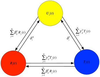
We refer to this model as the linear URTU model, because the rumor-spreading rates, โˆ‘j=1Nฮฒiโ€‹jUโ€‹Rjโ€‹(t)superscriptsubscript๐‘—1๐‘superscriptsubscript๐›ฝ๐‘–๐‘—๐‘ˆsubscript๐‘…๐‘—๐‘ก\sum_{j=1}^{N}\beta_{ij}^{U}R_{j}(t) and โˆ‘j=1Nฮฒiโ€‹jTโ€‹Rjโ€‹(t)superscriptsubscript๐‘—1๐‘superscriptsubscript๐›ฝ๐‘–๐‘—๐‘‡subscript๐‘…๐‘—๐‘ก\sum_{j=1}^{N}\beta_{ij}^{T}R_{j}(t), are linear in R1โ€‹(t),โ‹ฏ,RNโ€‹(t)subscript๐‘…1๐‘กโ‹ฏsubscript๐‘…๐‘๐‘กR_{1}(t),\cdots,R_{N}(t), and the truth-spreading rates, โˆ‘j=1Nฮณiโ€‹jUโ€‹Tjโ€‹(t)superscriptsubscript๐‘—1๐‘superscriptsubscript๐›พ๐‘–๐‘—๐‘ˆsubscript๐‘‡๐‘—๐‘ก\sum_{j=1}^{N}\gamma_{ij}^{U}T_{j}(t) and โˆ‘j=1Nฮณiโ€‹jRโ€‹Tjโ€‹(t)superscriptsubscript๐‘—1๐‘superscriptsubscript๐›พ๐‘–๐‘—๐‘…subscript๐‘‡๐‘—๐‘ก\sum_{j=1}^{N}\gamma_{ij}^{R}T_{j}(t), are linear in T1โ€‹(t),โ‹ฏ,TNโ€‹(t)subscript๐‘‡1๐‘กโ‹ฏsubscript๐‘‡๐‘๐‘กT_{1}(t),\cdots,T_{N}(t). See Fig. 2 for the state transition rates of a person under the linear URTU model.
Refer to caption
Figure 2: The state transition rates of person i๐‘–i under the linear URTU model.

The linear URTU model is a closed 3N๐‘N-dimensional dynamical system and is mathematically tractable. However, as the linear spreading rates may be different from the actual spreading rates, the dynamics of the model may deviate from the actual average dynamics of rumor-truth interaction.

2.5 The generic URTU model

For the purpose of approximating the exact URTU model more accurately, let us consider a more general rumor-truth spreading model as follows.

{dโ€‹Riโ€‹(t)dโ€‹t=(1โˆ’Riโ€‹(t)โˆ’Tiโ€‹(t))โ€‹fiUโ€‹(R1โ€‹(t),โ‹ฏ,RNโ€‹(t))โˆ’ฮดiRโ€‹Riโ€‹(t)+Tiโ€‹(t)โ€‹fiTโ€‹(R1โ€‹(t),โ‹ฏ,RNโ€‹(t))โˆ’Riโ€‹(t)โ€‹giRโ€‹(T1โ€‹(t),โ‹ฏ,TNโ€‹(t)),dโ€‹Tiโ€‹(t)dโ€‹t=(1โˆ’Riโ€‹(t)โˆ’Tiโ€‹(t))โ€‹giUโ€‹(T1โ€‹(t),โ‹ฏ,TNโ€‹(t))โˆ’ฮดiTโ€‹Tiโ€‹(t)+Riโ€‹(t)โ€‹giRโ€‹(T1โ€‹(t),โ‹ฏ,TNโ€‹(t))โˆ’Tiโ€‹(t)โ€‹fiTโ€‹(R1โ€‹(t),โ‹ฏ,RNโ€‹(t)),i=1,2,โ‹ฏ,N.\left\{\begin{aligned} \frac{dR_{i}(t)}{dt}&=\left(1-R_{i}(t)-T_{i}(t)\right)f_{i}^{U}\left(R_{1}(t),\cdots,R_{N}(t)\right)-\delta_{i}^{R}R_{i}(t)+T_{i}(t)f_{i}^{T}\left(R_{1}(t),\cdots,R_{N}(t)\right)-R_{i}(t)g_{i}^{R}(T_{1}(t),\cdots,T_{N}(t)),\\ \frac{dT_{i}(t)}{dt}&=\left(1-R_{i}(t)-T_{i}(t)\right)g_{i}^{U}\left(T_{1}(t),\cdots,T_{N}(t)\right)-\delta_{i}^{T}T_{i}(t)+R_{i}(t)g_{i}^{R}\left(T_{1}(t),\cdots,T_{N}(t)\right)-T_{i}(t)f_{i}^{T}(R_{1}(t),\cdots,R_{N}(t)),\\ &\quad\quad i=1,2,\cdots,N.\end{aligned}\right. (5)

Here, the spreading rates are assumed to satisfy the following generic conditions.

  1. (C1)

    (Proximity) An uncertain person or a truth-believer can and can only be influenced by those rumor-believers that can send the rumor to it through the rumor-spreading network. That is, fiUsuperscriptsubscript๐‘“๐‘–๐‘ˆf_{i}^{U} and fiTsuperscriptsubscript๐‘“๐‘–๐‘‡f_{i}^{T} is dependent upon xjsubscript๐‘ฅ๐‘—x_{j} if and only if (i,j)โˆˆER๐‘–๐‘—subscript๐ธ๐‘…(i,j)\in E_{R}. Likewise, An uncertain person or a rumor-believer can and can only be influenced by those truth-believers that can send the truth to it through the truth-spreading network. That is, giUsuperscriptsubscript๐‘”๐‘–๐‘ˆg_{i}^{U} and giRsuperscriptsubscript๐‘”๐‘–๐‘…g_{i}^{R} is dependent upon xjsubscript๐‘ฅ๐‘—x_{j} if and only if (i,j)โˆˆET๐‘–๐‘—subscript๐ธ๐‘‡(i,j)\in E_{T}.

  2. (C2)

    (Nullity) The rumor cannot spread unless there is a rumor-believer in the group. That is, fiUโ€‹(0,โ‹ฏ,0)=fiTโ€‹(0,โ‹ฏ,0)=0superscriptsubscript๐‘“๐‘–๐‘ˆ0โ‹ฏ0superscriptsubscript๐‘“๐‘–๐‘‡0โ‹ฏ00f_{i}^{U}(0,\cdots,0)=f_{i}^{T}(0,\cdots,0)=0. Likewise, the truth cannot spread unless there is a truth-believer in the group. That is, giUโ€‹(0,โ‹ฏ,0)=giRโ€‹(0,โ‹ฏ,0)=0superscriptsubscript๐‘”๐‘–๐‘ˆ0โ‹ฏ0superscriptsubscript๐‘”๐‘–๐‘…0โ‹ฏ00g_{i}^{U}(0,\cdots,0)=g_{i}^{R}(0,\cdots,0)=0.

  3. (C3)

    (Ordering) As compared to a truth-believer, an uncertain person is easier to believe the rumor. As compared to a rumor-believer, an uncertain person is easier to believe the truth. That is, fiUโ‰ฅfiTsuperscriptsubscript๐‘“๐‘–๐‘ˆsuperscriptsubscript๐‘“๐‘–๐‘‡f_{i}^{U}\geq f_{i}^{T}, giUโ‰ฅgiRsuperscriptsubscript๐‘”๐‘–๐‘ˆsuperscriptsubscript๐‘”๐‘–๐‘…g_{i}^{U}\geq g_{i}^{R}.

  4. (C4)

    (Smoothness) The spreading rates are sufficiently smooth. Technically speaking, fiUsuperscriptsubscript๐‘“๐‘–๐‘ˆf_{i}^{U}, fiTsuperscriptsubscript๐‘“๐‘–๐‘‡f_{i}^{T}, giUsuperscriptsubscript๐‘”๐‘–๐‘ˆg_{i}^{U} and giRsuperscriptsubscript๐‘”๐‘–๐‘…g_{i}^{R} are twice continuously differentible.

  5. (C5)

    (Monotonicity) The spreading rates are strictly increasing with respect to every relevant argument. That is, โˆ‚fiUโ€‹(x1,โ‹ฏ,xN)โˆ‚xj>0superscriptsubscript๐‘“๐‘–๐‘ˆsubscript๐‘ฅ1โ‹ฏsubscript๐‘ฅ๐‘subscript๐‘ฅ๐‘—0\frac{\partial f_{i}^{U}(x_{1},\cdots,x_{N})}{\partial x_{j}}>0 if fiUsuperscriptsubscript๐‘“๐‘–๐‘ˆf_{i}^{U} is dependent upon xjsubscript๐‘ฅ๐‘—x_{j}, โˆ‚fiTโ€‹(x1,โ‹ฏ,xN)โˆ‚xj>0superscriptsubscript๐‘“๐‘–๐‘‡subscript๐‘ฅ1โ‹ฏsubscript๐‘ฅ๐‘subscript๐‘ฅ๐‘—0\frac{\partial f_{i}^{T}(x_{1},\cdots,x_{N})}{\partial x_{j}}>0 if fiTsuperscriptsubscript๐‘“๐‘–๐‘‡f_{i}^{T} is dependent upon xjsubscript๐‘ฅ๐‘—x_{j}, โˆ‚giUโ€‹(x1,โ‹ฏ,xN)โˆ‚xj>0superscriptsubscript๐‘”๐‘–๐‘ˆsubscript๐‘ฅ1โ‹ฏsubscript๐‘ฅ๐‘subscript๐‘ฅ๐‘—0\frac{\partial g_{i}^{U}(x_{1},\cdots,x_{N})}{\partial x_{j}}>0 if giUsuperscriptsubscript๐‘”๐‘–๐‘ˆg_{i}^{U} is dependent upon xjsubscript๐‘ฅ๐‘—x_{j}, and โˆ‚giRโ€‹(x1,โ‹ฏ,xN)โˆ‚xj>0superscriptsubscript๐‘”๐‘–๐‘…subscript๐‘ฅ1โ‹ฏsubscript๐‘ฅ๐‘subscript๐‘ฅ๐‘—0\frac{\partial g_{i}^{R}(x_{1},\cdots,x_{N})}{\partial x_{j}}>0 if giRsuperscriptsubscript๐‘”๐‘–๐‘…g_{i}^{R} is dependent upon xjsubscript๐‘ฅ๐‘—x_{j}.

  6. (C6)

    (Concavity) The spreading rates flatten out and tend to saturation. That is, โˆ‚2fiUโ€‹(x1,โ‹ฏ,xN)โˆ‚xjโ€‹โˆ‚xkโ‰ค0superscript2superscriptsubscript๐‘“๐‘–๐‘ˆsubscript๐‘ฅ1โ‹ฏsubscript๐‘ฅ๐‘subscript๐‘ฅ๐‘—subscript๐‘ฅ๐‘˜0\frac{\partial^{2}f_{i}^{U}(x_{1},\cdots,x_{N})}{\partial x_{j}\partial x_{k}}\leq 0, โˆ‚2fiTโ€‹(x1,โ‹ฏ,xN)โˆ‚xjโ€‹โˆ‚xkโ‰ค0superscript2superscriptsubscript๐‘“๐‘–๐‘‡subscript๐‘ฅ1โ‹ฏsubscript๐‘ฅ๐‘subscript๐‘ฅ๐‘—subscript๐‘ฅ๐‘˜0\frac{\partial^{2}f_{i}^{T}(x_{1},\cdots,x_{N})}{\partial x_{j}\partial x_{k}}\leq 0, โˆ‚2giUโ€‹(x1,โ‹ฏ,xN)โˆ‚xjโ€‹โˆ‚xkโ‰ค0superscript2superscriptsubscript๐‘”๐‘–๐‘ˆsubscript๐‘ฅ1โ‹ฏsubscript๐‘ฅ๐‘subscript๐‘ฅ๐‘—subscript๐‘ฅ๐‘˜0\frac{\partial^{2}g_{i}^{U}(x_{1},\cdots,x_{N})}{\partial x_{j}\partial x_{k}}\leq 0, and โˆ‚2giRโ€‹(x1,โ‹ฏ,xN)โˆ‚xjโ€‹โˆ‚xkโ‰ค0superscript2superscriptsubscript๐‘”๐‘–๐‘…subscript๐‘ฅ1โ‹ฏsubscript๐‘ฅ๐‘subscript๐‘ฅ๐‘—subscript๐‘ฅ๐‘˜0\frac{\partial^{2}g_{i}^{R}(x_{1},\cdots,x_{N})}{\partial x_{j}\partial x_{k}}\leq 0.

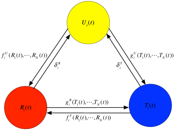
We refer to model (5) as the generic URTU model. See Fig. 3 for the state transition rates of a person under the generic URTU model. Obviously, this model subsumes the linear URTU model as well as many other URTU models with nonlinear spreading rates.
Refer to caption
Figure 3: The state transition rates of person i๐‘–i under the generic URTU model.

Let

ฮฉ={(x1,โ‹ฏ,x2โ€‹N)โˆˆโ„+2โ€‹Nโˆฃxi+xN+iโ‰ค1,1โ‰คiโ‰คN}.ฮฉconditional-setsubscript๐‘ฅ1โ‹ฏsubscript๐‘ฅ2๐‘superscriptsubscriptโ„2๐‘formulae-sequencesubscript๐‘ฅ๐‘–subscript๐‘ฅ๐‘๐‘–11๐‘–๐‘\Omega=\left\{(x_{1},\cdots,x_{2N})\in\mathbb{R}_{+}^{2N}\mid x_{i}+x_{N+i}\leq 1,1\leq i\leq N\right\}.

The initial state of model (5) lies in ฮฉฮฉ\Omega. It is easily shown that ฮฉฮฉ\Omega is positively invariant for model (5).

Let us introduce the following matrix-vector notations.

๐‘โ€‹(t)=(R1โ€‹(t),โ‹ฏ,RNโ€‹(t))T,๐“โ€‹(t)=(T1โ€‹(t),โ‹ฏ,TNโ€‹(t))T,formulae-sequence๐‘๐‘กsuperscriptsubscript๐‘…1๐‘กโ‹ฏsubscript๐‘…๐‘๐‘ก๐‘‡๐“๐‘กsuperscriptsubscript๐‘‡1๐‘กโ‹ฏsubscript๐‘‡๐‘๐‘ก๐‘‡\mathbf{R}(t)=(R_{1}(t),\cdots,R_{N}(t))^{T},\quad\mathbf{T}(t)=(T_{1}(t),\cdots,T_{N}(t))^{T},
dโ€‹iโ€‹aโ€‹gโ€‹๐‘โ€‹(t)=dโ€‹iโ€‹aโ€‹gโ€‹(Riโ€‹(t)),dโ€‹iโ€‹aโ€‹gโ€‹๐“โ€‹(t)=dโ€‹iโ€‹aโ€‹gโ€‹(Tiโ€‹(t)),formulae-sequence๐‘‘๐‘–๐‘Ž๐‘”๐‘๐‘ก๐‘‘๐‘–๐‘Ž๐‘”subscript๐‘…๐‘–๐‘ก๐‘‘๐‘–๐‘Ž๐‘”๐“๐‘ก๐‘‘๐‘–๐‘Ž๐‘”subscript๐‘‡๐‘–๐‘กdiag\mathbf{R}(t)=diag\left(R_{i}(t)\right),\quad diag\mathbf{T}(t)=diag\left(T_{i}(t)\right),
๐ŸUโ€‹(๐‘โ€‹(t))=(f1Uโ€‹(๐‘โ€‹(t)),โ‹ฏ,fNUโ€‹(๐‘โ€‹(t)))T,๐ŸTโ€‹(๐‘โ€‹(t))=(f1Tโ€‹(๐‘โ€‹(t)),โ‹ฏ,fNTโ€‹(๐‘โ€‹(t)))T,๐ Uโ€‹(๐“โ€‹(t))=(g1Uโ€‹(๐“โ€‹(t)),โ‹ฏ,gNUโ€‹(๐“โ€‹(t)))T,๐ Rโ€‹(๐“โ€‹(t))=(g1Rโ€‹(๐“โ€‹(t)),โ‹ฏ,gNRโ€‹(๐“โ€‹(t)))T.\begin{split}\mathbf{f}_{U}(\mathbf{R}(t))&=\left(f_{1}^{U}(\mathbf{R}(t)),\cdots,f_{N}^{U}(\mathbf{R}(t))\right)^{T},\quad\mathbf{f}_{T}(\mathbf{R}(t))=\left(f_{1}^{T}(\mathbf{R}(t)),\cdots,f_{N}^{T}(\mathbf{R}(t))\right)^{T},\\ \mathbf{g}_{U}(\mathbf{T}(t))&=\left(g_{1}^{U}(\mathbf{T}(t)),\cdots,g_{N}^{U}(\mathbf{T}(t))\right)^{T},\quad\mathbf{g}_{R}(\mathbf{T}(t))=\left(g_{1}^{R}(\mathbf{T}(t)),\cdots,g_{N}^{R}(\mathbf{T}(t))\right)^{T}.\end{split}

Then the generic URTU model can be written as

{dโ€‹๐‘โ€‹(t)dโ€‹t=(๐„Nโˆ’dโ€‹iโ€‹aโ€‹gโ€‹๐‘โ€‹(t)โˆ’dโ€‹iโ€‹aโ€‹gโ€‹๐“โ€‹(t))โ€‹๐ŸUโ€‹(๐‘โ€‹(t))โˆ’๐ƒRโ€‹๐‘โ€‹(t)+dโ€‹iโ€‹aโ€‹gโ€‹๐“โ€‹(t)โ€‹๐ŸTโ€‹(๐‘โ€‹(t))โˆ’dโ€‹iโ€‹aโ€‹gโ€‹๐‘โ€‹(t)โ€‹๐ Rโ€‹(๐“โ€‹(t)),dโ€‹๐“โ€‹(t)dโ€‹t=(๐„Nโˆ’dโ€‹iโ€‹aโ€‹gโ€‹๐‘โ€‹(t)โˆ’dโ€‹iโ€‹aโ€‹gโ€‹๐“โ€‹(t))โ€‹๐ Uโ€‹(๐“โ€‹(t))โˆ’๐ƒTโ€‹๐“โ€‹(t)+dโ€‹iโ€‹aโ€‹gโ€‹๐‘โ€‹(t)โ€‹๐ Rโ€‹(๐“โ€‹(t))โˆ’dโ€‹iโ€‹aโ€‹gโ€‹๐“โ€‹(t)โ€‹๐ŸRโ€‹(๐‘โ€‹(t)),\left\{\begin{aligned} \frac{d\mathbf{R}(t)}{dt}&=(\mathbf{E}_{N}-diag\mathbf{R}(t)-diag\mathbf{T}(t))\mathbf{f}_{U}(\mathbf{R}(t))-\mathbf{D}_{R}\mathbf{R}(t)+diag\mathbf{T}(t)\mathbf{f}_{T}(\mathbf{R}(t))-diag\mathbf{R}(t)\mathbf{g}_{R}(\mathbf{T}(t)),\\ \frac{d\mathbf{T}(t)}{dt}&=(\mathbf{E}_{N}-diag\mathbf{R}(t)-diag\mathbf{T}(t))\mathbf{g}_{U}(\mathbf{T}(t))-\mathbf{D}_{T}\mathbf{T}(t)+diag\mathbf{R}(t)\mathbf{g}_{R}(\mathbf{T}(t))-diag\mathbf{T}(t)\mathbf{f}_{R}(\mathbf{R}(t)),\end{aligned}\right. (6)

where ๐„Nsubscript๐„๐‘\mathbf{E}_{N} stands for the identity matrix of order N๐‘N.

3 Dynamics of the generic URTU model

Consider the generic URTU model (5). Let Rโ€‹(t)๐‘…๐‘กR(t) and Tโ€‹(t)๐‘‡๐‘กT(t) denote the fraction at time t๐‘กt of rumor-believers and truth-believers, respectively. That is,

Rโ€‹(t)=1Nโ€‹โˆ‘i=1NRiโ€‹(t),Tโ€‹(t)=1Nโ€‹โˆ‘i=1NTiโ€‹(t).formulae-sequence๐‘…๐‘ก1๐‘superscriptsubscript๐‘–1๐‘subscript๐‘…๐‘–๐‘ก๐‘‡๐‘ก1๐‘superscriptsubscript๐‘–1๐‘subscript๐‘‡๐‘–๐‘กR(t)=\frac{1}{N}\sum_{i=1}^{N}R_{i}(t),\quad T(t)=\frac{1}{N}\sum_{i=1}^{N}T_{i}(t). (7)

The main aim of this work is to determine the developing tendency of Rโ€‹(t)๐‘…๐‘กR(t) and Tโ€‹(t)๐‘‡๐‘กT(t) over time. For that purpose, we need some preliminary knowledges, which are listed below.

3.1 Preliminaries

For fundamental knowledge on matrix theory, see Ref. [50]. In what follows, we consider only real square matrices. Given a matrix ๐€๐€\mathbf{A}, let sโ€‹(๐€)๐‘ ๐€s(\mathbf{A}) denote the maximum real part of an eigenvalue of ๐€๐€\mathbf{A}, and let ฯโ€‹(๐€)๐œŒ๐€\rho(\mathbf{A}) denote the spectral radius of ๐€๐€\mathbf{A}, i.e., the maximum modulus of an eigenvalue of ๐€๐€\mathbf{A}. ๐€๐€\mathbf{A} is Metzler if its off-diagonal entries are all nonnegative.

Lemma 2.

(Corollary 8.1.30 in [50]) Let ๐€๐€\mathbf{A} be a nonnegative matrix. If ๐€๐€\mathbf{A} has a positive eigenvector ๐ฑ๐ฑ\mathbf{x}, then ฯโ€‹(๐€)๐œŒ๐€\rho(\mathbf{A}) is an eigenvalue of ๐€๐€\mathbf{A}, and ๐ฑ๐ฑ\mathbf{x} belongs to ฯโ€‹(๐€)๐œŒ๐€\rho(\mathbf{A}).

Lemma 3.

(Lemma 2.3 in [51]) Let ๐€๐€\mathbf{A} be an irreducible Metzler matrix. Then sโ€‹(๐€)๐‘ ๐€s(\mathbf{A}) is a simple eigenvalue of ๐€๐€\mathbf{A}, and, up to scalar multiple, ๐€๐€\mathbf{A} has a unique positive eigenvector ๐ฑ๐ฑ\mathbf{x} belonging to sโ€‹(๐€)๐‘ ๐€s(\mathbf{A}).

A matrix ๐€๐€\mathbf{A} is Hurwitz stable or simply Hurwitz if its eigenvalues all have negative real parts, i.e., sโ€‹(๐€)<0๐‘ ๐€0s(\mathbf{A})<0.

Lemma 4.

(Chapter 2 in [52]) A matrix ๐€๐€\mathbf{A} is Hurwitz if and only if there is a positive definite matrix ๐๐\mathbf{P} such that ๐€Tโ€‹๐+๐๐€superscript๐€๐‘‡๐๐๐€\mathbf{A}^{T}\mathbf{P}+\mathbf{P}\mathbf{A} is negative definite.

A matrix ๐€๐€\mathbf{A} is diagonally stable if there is a positive definite diagonal matrix ๐ƒ๐ƒ\mathbf{D} such that ๐€Tโ€‹๐ƒ+๐ƒ๐€superscript๐€๐‘‡๐ƒ๐ƒ๐€\mathbf{A}^{T}\mathbf{D}+\mathbf{D}\mathbf{A} is negative definite. Obviously, a diagonally stable matrix is Hurwitz.

Lemma 5.

(Section 2 in [53]) A Metzler matrix is diagonally stable if it is Hurwitz.

Lemma 6.

(Lemma A.1 in [54]) Let ๐€๐€\mathbf{A} be an irreducible Metzler matrix. If sโ€‹(๐€)=0๐‘ ๐€0s(\mathbf{A})=0, then there is a positive definite diagonal matrix ๐ƒ๐ƒ\mathbf{D} such that ๐€Tโ€‹๐ƒ+๐ƒ๐€superscript๐€๐‘‡๐ƒ๐ƒ๐€\mathbf{A}^{T}\mathbf{D}+\mathbf{D}\mathbf{A} is negative semi-definite.

For fundamental theory on differential dynamical systems, see Ref. [55].

Lemma 7.

(Chaplygin Lemma, see Theorem 31.4 in [56]) Consider a smooth n๐‘›n-dimensional system of differential equations

dโ€‹๐ฑโ€‹(t)dโ€‹t=๐Ÿ((๐ฑ(t)),tโ‰ฅ0\frac{d\mathbf{x}(t)}{dt}=\mathbf{f}(\mathbf{(}\mathbf{x}(t)),\quad t\geq 0

and the corresponding system of differential inequalities

dโ€‹๐ฒโ€‹(t)dโ€‹tโ‰ค๐Ÿ((๐ฒ(t)),tโ‰ฅ0\frac{d\mathbf{y}(t)}{dt}\leq\mathbf{f}(\mathbf{(}\mathbf{y}(t)),\quad t\geq 0

with ๐ฑโ€‹(0)=๐ฒโ€‹(0)๐ฑ0๐ฒ0\mathbf{x}(0)=\mathbf{y}(0). Suppose that for any a1,โ‹ฏ,anโ‰ฅ0subscript๐‘Ž1โ‹ฏsubscript๐‘Ž๐‘›0a_{1},\cdots,a_{n}\geq 0, there hold

fiโ€‹(x1+a1,โ‹ฏ,xiโˆ’1+aiโˆ’1,xi,xi+1+ai+1,โ‹ฏ,xn+an)โ‰ฅfiโ€‹(x1,โ‹ฏ,xn),i=1,โ‹ฏ,n.formulae-sequencesubscript๐‘“๐‘–subscript๐‘ฅ1subscript๐‘Ž1โ‹ฏsubscript๐‘ฅ๐‘–1subscript๐‘Ž๐‘–1subscript๐‘ฅ๐‘–subscript๐‘ฅ๐‘–1subscript๐‘Ž๐‘–1โ‹ฏsubscript๐‘ฅ๐‘›subscript๐‘Ž๐‘›subscript๐‘“๐‘–subscript๐‘ฅ1โ‹ฏsubscript๐‘ฅ๐‘›๐‘–1โ‹ฏ๐‘›f_{i}(x_{1}+a_{1},\cdots,x_{i-1}+a_{i-1},x_{i},x_{i+1}+a_{i+1},\cdots,x_{n}+a_{n})\geq f_{i}(x_{1},\cdots,x_{n}),\quad i=1,\cdots,n.

Then ๐ฒโ€‹(t)โ‰ค๐ฑโ€‹(t),tโ‰ฅ0formulae-sequence๐ฒ๐‘ก๐ฑ๐‘ก๐‘ก0\mathbf{y}(t)\leq\mathbf{x}(t),t\geq 0.

Lemma 8.

(Strauss-Yorke Theorem, see Corollary 3.3 in [57]) Consider a differential dynamical system

dโ€‹๐ฑโ€‹(t)dโ€‹t=๐Ÿ((๐ฑ(t))+๐ (t,๐ฑ(t)),tโ‰ฅ0,\frac{d\mathbf{x}(t)}{dt}=\mathbf{f}(\mathbf{(}\mathbf{x}(t))+\mathbf{g}(t,\mathbf{x}(t)),\quad t\geq 0,

with ๐ โ€‹(t,๐ฑโ€‹(t))โ†’๐ŸŽโ†’๐ ๐‘ก๐ฑ๐‘ก0\mathbf{g}(t,\mathbf{x}(t))\rightarrow\mathbf{0} when tโ†’โˆžโ†’๐‘กt\rightarrow\infty. Let

dโ€‹๐ฒโ€‹(t)dโ€‹t=๐Ÿ((๐ฒ(t)),tโ‰ฅ0\frac{d\mathbf{y}(t)}{dt}=\mathbf{f}(\mathbf{(}\mathbf{y}(t)),\quad t\geq 0

denote the limit system of this system. If the origin is a global attractor for the limit system, and every solution to the original system is bounded on [0,โˆž)0[0,\infty), then the origin is also a global attractor for the original system.

For fundamental knowledge on fixed point theory, see Ref. [58].

Lemma 9.

(Brouwer Fixed Point Theorem, see Theorem 4.10 in [58]) Let CโŠ‚โ„n๐ถsuperscriptโ„๐‘›C\subset\mathbb{R}^{n} be nonempty, bounded, closed, and convex. Let f:Cโ†’C:๐‘“โ†’๐ถ๐ถf:C\rightarrow C be a continuous function. Then f๐‘“f has a fixed point.

3.2 The equilibria

The first step to understanding the dynamics of a differential dynamical system is to examine all of its equilibria. The generic URTU model might admit four different types of equilibria, which are defined as follows.

Definition 1.

Let ๐„=(๐‘T,๐“T)T๐„superscriptsuperscript๐‘๐‘‡superscript๐“๐‘‡๐‘‡\mathbf{E}=(\mathbf{R}^{T},\mathbf{T}^{T})^{T} be an equilibrium of the generic URTU model.

  1. (a)

    ๐„๐„\mathbf{E} is uncertain if ๐‘=๐“=๐ŸŽ๐‘๐“0\mathbf{R}=\mathbf{T}=\mathbf{0}, which stands for the steady OSN state in which all persons are uncertain almost surely.

  2. (b)

    ๐„๐„\mathbf{E} is rumor-dominant if ๐‘โ‰ ๐ŸŽ๐‘0\mathbf{R}\neq\mathbf{0} and ๐“=๐ŸŽ๐“0\mathbf{T}=\mathbf{0}, which stands for a steady OSN state in which some persons believe the rumor with positive probability and no person believes the truth almost surely.

  3. (c)

    ๐„๐„\mathbf{E} is truth-dominant if ๐‘=๐ŸŽ๐‘0\mathbf{R}=\mathbf{0} and ๐“โ‰ ๐ŸŽ๐“0\mathbf{T}\neq\mathbf{0}, which stands for a steady OSN state in which some persons believe the truth with positive probability and no person believes the rumor almost surely.

  4. (d)

    ๐„๐„\mathbf{E} is coexistent if ๐‘โ‰ ๐ŸŽ๐‘0\mathbf{R}\neq\mathbf{0} and ๐“โ‰ ๐ŸŽ๐“0\mathbf{T}\neq\mathbf{0}, which stands for a steady OSN state in which some persons believe the rumor with positive probability and some persons believe the truth with positive probability.

Obviously, the generic URTU model always admits the uncertain equilibrium ๐„U=(0,โ‹ฏ,0)Tsubscript๐„๐‘ˆsuperscript0โ‹ฏ0๐‘‡\mathbf{E}_{U}=(0,\cdots,0)^{T}. Due to the complexity of the model, we are unable to figure out its other equilibria. For our purpose, define a pair of Metzler matrices as follows.

๐1=โˆ‚๐ŸUโ€‹(๐ŸŽ)โˆ‚๐ฑโˆ’๐ƒR,๐2=โˆ‚๐ Uโ€‹(๐ŸŽ)โˆ‚๐ฑโˆ’๐ƒT,formulae-sequencesubscript๐1subscript๐Ÿ๐‘ˆ0๐ฑsubscript๐ƒ๐‘…subscript๐2subscript๐ ๐‘ˆ0๐ฑsubscript๐ƒ๐‘‡\mathbf{Q}_{1}=\frac{\partial\mathbf{f}_{U}(\mathbf{0})}{\partial\mathbf{x}}-\mathbf{D}_{R},\quad\mathbf{Q}_{2}=\frac{\partial\mathbf{g}_{U}(\mathbf{0})}{\partial\mathbf{x}}-\mathbf{D}_{T}, (8)

where โˆ‚๐ŸUโ€‹(๐ŸŽ)โˆ‚๐ฑsubscript๐Ÿ๐‘ˆ0๐ฑ\frac{\partial\mathbf{f}_{U}(\mathbf{0})}{\partial\mathbf{x}} and โˆ‚๐ Uโ€‹(๐ŸŽ)โˆ‚๐ฑsubscript๐ ๐‘ˆ0๐ฑ\frac{\partial\mathbf{g}_{U}(\mathbf{0})}{\partial\mathbf{x}} stand for the Jacobian matrix of ๐ŸUsubscript๐Ÿ๐‘ˆ\mathbf{f}_{U} and ๐ Usubscript๐ ๐‘ˆ\mathbf{g}_{U} evaluated at the origin, respectively. As GRsubscript๐บ๐‘…G_{R} and GTsubscript๐บ๐‘‡G_{T} are strongly connected, the four matrices are all irreducible.

We are ready to present the following fundamental result about the equilibria of the generic URTU model.

Theorem 1.

Consider model (5). The following claims hold.

  1. (a)

    If sโ€‹(๐1)>0๐‘ subscript๐10s(\mathbf{Q}_{1})>0, then the model admits a unique rumor-dominant equilibrium. Let ๐„R=(๐‘T,๐ŸŽT)Tsubscript๐„๐‘…superscriptsuperscript๐‘๐‘‡superscript0๐‘‡๐‘‡\mathbf{E}_{R}=(\mathbf{R}^{T},\mathbf{0}^{T})^{T} denote the equilibrium, then ๐ŸŽ<๐‘<๐Ÿ0๐‘1\mathbf{0}<\mathbf{R}<\mathbf{1}.

  2. (b)

    If sโ€‹(๐2)>0๐‘ subscript๐20s(\mathbf{Q}_{2})>0, then the model admits a unique truth-dominant equilibrium. Let ๐„T=(๐ŸŽT,๐“T)Tsubscript๐„๐‘‡superscriptsuperscript0๐‘‡superscript๐“๐‘‡๐‘‡\mathbf{E}_{T}=(\mathbf{0}^{T},\mathbf{T}^{T})^{T} denote the equilibrium, then ๐ŸŽ<๐“<๐Ÿ0๐“1\mathbf{0}<\mathbf{T}<\mathbf{1}.

The proof of the theorem is left to Appendix B. This theorem manifests that the existence and locations of equilibria of the generic URTU model are dependent in a complex way upon the basic parameters as well as the network structures.

3.3 Attractivity analysis

Now, let us examine the attractivity of the equilibria of the generic URTU model. First, we have the following criterion for the attractivity of the uncertain equilibrium.

Theorem 2.

Consider model (5). Suppose sโ€‹(๐1)โ‰ค0๐‘ subscript๐10s(\mathbf{Q}_{1})\leq 0 and sโ€‹(๐2)โ‰ค0๐‘ subscript๐20s(\mathbf{Q}_{2})\leq 0. Then the uncertain equilibrium ๐„Usubscript๐„๐‘ˆ\mathbf{E}_{U} attracts ฮฉฮฉ\Omega. Hence, Rโ€‹(t)โ†’0โ†’๐‘…๐‘ก0R(t)\rightarrow 0 and Tโ€‹(t)โ†’0โ†’๐‘‡๐‘ก0T(t)\rightarrow 0 as tโ†’โˆžโ†’๐‘กt\rightarrow\infty.

The proof of the theorem is left to Appendix C. This theorem has the following useful corollary.

Corollary 1.

The uncertain equilibrium ๐„Usubscript๐„๐‘ˆ\mathbf{E}_{U} of model (5) attracts ฮฉฮฉ\Omega if one of the following conditions is satisfied.

  1. (a)

    ฯโ€‹(๐1โ€‹๐ƒRโˆ’1+๐„N)<1๐œŒsubscript๐1superscriptsubscript๐ƒ๐‘…1subscript๐„๐‘1\rho(\mathbf{Q}_{1}\mathbf{D}_{R}^{-1}+\mathbf{E}_{N})<1, ฯโ€‹(๐2โ€‹๐ƒTโˆ’1+๐„N)<1๐œŒsubscript๐2superscriptsubscript๐ƒ๐‘‡1subscript๐„๐‘1\rho(\mathbf{Q}_{2}\mathbf{D}_{T}^{-1}+\mathbf{E}_{N})<1.

  2. (b)

    ฯโ€‹(๐Uโ€‹๐ƒRโˆ’1)<1๐œŒsubscript๐๐‘ˆsuperscriptsubscript๐ƒ๐‘…11\rho(\mathbf{B}_{U}\mathbf{D}_{R}^{-1})<1, ฯโ€‹(๐‚Uโ€‹๐ƒTโˆ’1)<1๐œŒsubscript๐‚๐‘ˆsuperscriptsubscript๐ƒ๐‘‡11\rho(\mathbf{C}_{U}\mathbf{D}_{T}^{-1})<1.

  3. (c)

    โˆ‘i=1Nฮฒiโ€‹jU<ฮดjRsuperscriptsubscript๐‘–1๐‘superscriptsubscript๐›ฝ๐‘–๐‘—๐‘ˆsuperscriptsubscript๐›ฟ๐‘—๐‘…\sum_{i=1}^{N}\beta_{ij}^{U}<\delta_{j}^{R}, โˆ‘i=1Nฮณiโ€‹jU<ฮดjTsuperscriptsubscript๐‘–1๐‘superscriptsubscript๐›พ๐‘–๐‘—๐‘ˆsuperscriptsubscript๐›ฟ๐‘—๐‘‡\sum_{i=1}^{N}\gamma_{ij}^{U}<\delta_{j}^{T}, j=1,2โ€‹โ‹ฏ,N๐‘—12โ‹ฏ๐‘j=1,2\cdots,N.

  4. (d)

    โˆ‘j=1Nฮฒiโ€‹jUฮดjR<1superscriptsubscript๐‘—1๐‘superscriptsubscript๐›ฝ๐‘–๐‘—๐‘ˆsuperscriptsubscript๐›ฟ๐‘—๐‘…1\sum_{j=1}^{N}\frac{\beta_{ij}^{U}}{\delta_{j}^{R}}<1, โˆ‘j=1Nฮณiโ€‹jUฮดjT<1superscriptsubscript๐‘—1๐‘superscriptsubscript๐›พ๐‘–๐‘—๐‘ˆsuperscriptsubscript๐›ฟ๐‘—๐‘‡1\sum_{j=1}^{N}\frac{\gamma_{ij}^{U}}{\delta_{j}^{T}}<1, i=1,2,โ‹ฏ,N๐‘–12โ‹ฏ๐‘i=1,2,\cdots,N.

The proof of this corollary is left to Appendix D. The following theorem offers a criterion for the global attractivity of the rumor-dominant equilibrium.

Theorem 3.

Consider model (5). Suppose sโ€‹(๐1)>0๐‘ subscript๐10s(\mathbf{Q}_{1})>0 and sโ€‹(๐2)โ‰ค0๐‘ subscript๐20s(\mathbf{Q}_{2})\leq 0. Then the rumor-dominant equilibrium ๐„Rsubscript๐„๐‘…\mathbf{E}_{R} attracts {(๐‘,๐“)โˆˆฮฉ:๐‘โ‰ ๐ŸŽ}conditional-set๐‘๐“ฮฉ๐‘0\{(\mathbf{R},\mathbf{T})\in\Omega:\mathbf{R}\neq\mathbf{0}\}. Hence, if Rโ€‹(0)โ‰ 0๐‘…00R(0)\neq 0, then Rโ€‹(t)โ†’Rโˆ—โ†’๐‘…๐‘กsuperscript๐‘…R(t)\rightarrow R^{*} and Tโ€‹(t)โ†’0โ†’๐‘‡๐‘ก0T(t)\rightarrow 0 as tโ†’โˆžโ†’๐‘กt\rightarrow\infty.

The proof of the theorem is left to Appendix E. In parallel, we have the following criterion for the attractivity of the truth-dominant equilibrium.

Theorem 4.

Consider model (5). Suppose sโ€‹(๐1)โ‰ค0๐‘ subscript๐10s(\mathbf{Q}_{1})\leq 0 and sโ€‹(๐2)>0๐‘ subscript๐20s(\mathbf{Q}_{2})>0. Then the truth-dominant equilibrium ๐„Tsubscript๐„๐‘‡\mathbf{E}_{T} attracts {(๐‘,๐“)โˆˆฮฉ:๐“โ‰ ๐ŸŽ}conditional-set๐‘๐“ฮฉ๐“0\{(\mathbf{R},\mathbf{T})\in\Omega:\mathbf{T}\neq\mathbf{0}\}. Hence, if Tโ€‹(0)โ‰ 0๐‘‡00T(0)\neq 0, then Rโ€‹(t)โ†’0โ†’๐‘…๐‘ก0R(t)\rightarrow 0 and Tโ€‹(t)โ†’Tโˆ—โ†’๐‘‡๐‘กsuperscript๐‘‡T(t)\rightarrow T^{*} as tโ†’โˆžโ†’๐‘กt\rightarrow\infty.

The argument for the theorem is analogous to that for Theorem 3 and hence is omitted.

Theorems 2 and 4 demonstrate that when (a) sโ€‹(๐1)โ‰ค0๐‘ subscript๐10s(\mathbf{Q}_{1})\leq 0 and sโ€‹(๐2)โ‰ค0๐‘ subscript๐20s(\mathbf{Q}_{2})\leq 0, or (b) sโ€‹(๐1)โ‰ค0๐‘ subscript๐10s(\mathbf{Q}_{1})\leq 0, sโ€‹(๐2)>0๐‘ subscript๐20s(\mathbf{Q}_{2})>0 and Tโ€‹(0)โ‰ 0๐‘‡00T(0)\neq 0, the rumor would terminate. In practice, the following measures are recommended to inhibit rumors.

  1. (a)

    Enhance the truth-spreading rates by presenting a convincing truth elaboration as early as possible.

  2. (b)

    Reduce the rumor-spreading rates by pointing out irrational aspects of the rumor.

  3. (c)

    Expand channels of spreading truths such as mass media and official announcement.

  4. (d)

    Lessen channels of spreading rumors by improving the quality of people.

4 Accuracy of the linear URTU model

As was mentioned in Section 2, the exact URTU model accurately captures the average dynamics of the rumor-truth interaction, while the linear URTU model is an approximation of the exact URTU model. A question arises naturally: under what conditions does the linear URTU model satisfactorily capture this averaged dynamics? This section is devoted to giving an answer to the question via computer simulations.

For the comparison purpose, we need to numerically solve the exact URTU model, because its closed-form solution is far beyond our reach. Based on the standard Gillespie algorithm for numerically solving continuous-time Markov chain models [59], we develop a numerical algorithm for solving the exact URTU model. The basic idea of the algorithm is to take the average of M=104๐‘€superscript104M=10^{4} sample paths of the original URTU model as the solution to the exact URTU model. In the following experiments, a randomly chosen person is initialized as rumor-believing, a randomly chosen person is initialized as truth-believing, and all the remaining persons in the OSN are initialized as uncertain.

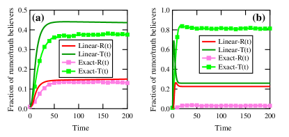
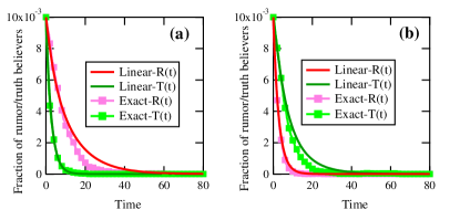
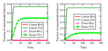
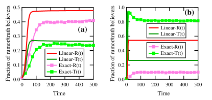
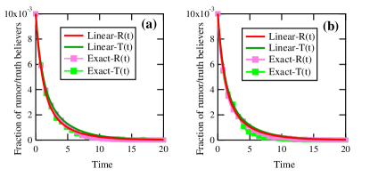
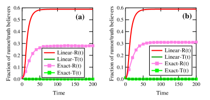
Scale-free networks are a large class of networks having widespread applications [20]. Take a randomly generated scale-free network with 100 nodes as the rumor-spreading network as well as the truth-spreading network. By taking random combinations of the parameters, we get 4096 pairs of linear and exact URTU models, which are divided into four collections: 94 pairs for each of which Rโ€‹(t)๐‘…๐‘กR(t) and Tโ€‹(t)๐‘‡๐‘กT(t) approach zero simultaneously, 1764 pairs for each of which Rโ€‹(t)๐‘…๐‘กR(t) approaches a nonzero value but Tโ€‹(t)๐‘‡๐‘กT(t) approaches zero, 1770 pairs for each of which Rโ€‹(t)๐‘…๐‘กR(t) approaches zero but Tโ€‹(t)๐‘‡๐‘กT(t) approaches a nonzero value, and 468 pairs for each of which both Rโ€‹(t)๐‘…๐‘กR(t) and Tโ€‹(t)๐‘‡๐‘กT(t) approach nonzero values. By observation, we find that, for each of the four collections of pairs, the way that the dynamics of a linear URTU model deviates from that of the paired exact URTU model is qualitatively similar. Figs. 4-7 give the comparison results of two pairs for each collection, respectively.
Refer to caption
Figure 4: Comparison results for two pairs in the first collection.
Refer to caption
Figure 5: Comparison results for two pairs in the second collection.
Refer to caption
Figure 6: Comparison results for two pairs in the third collection.
Refer to caption
Figure 7: Comparison results for two pairs in the fourth collection.

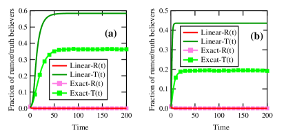
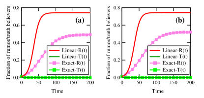
Small-world networks are another large class of networks having widespread applications [60]. Take a randomly generated small-word network with 100 nodes as the rumor-spreading network and the truth-distributing network. By taking random combinations of the parameters, we get 4096 pairs of linear and exact URTU models, which are divided into four collections: 151 pairs for each of which Rโ€‹(t)๐‘…๐‘กR(t) and Tโ€‹(t)๐‘‡๐‘กT(t) approach zero simultaneously, 1657 pairs for each of which Rโ€‹(t)๐‘…๐‘กR(t) approaches a nonzero value but Tโ€‹(t)๐‘‡๐‘กT(t) approaches zero, 1639 pairs for each of which Rโ€‹(t)๐‘…๐‘กR(t) approaches zero but Tโ€‹(t)๐‘‡๐‘กT(t) approaches a nonzero value, and 649 pairs for each of which both Rโ€‹(t)๐‘…๐‘กR(t) and Tโ€‹(t)๐‘‡๐‘กT(t) approach nonzero values. By observation, we find that, for each of the four collections of pairs, the way that the dynamics of a linear URTU model deviates from that of the paired exact URTU model is qualitatively similar. Figs. 8-11 give the comparison results of two pairs for each collection, respectively.
Refer to caption
Figure 8: Comparison results for two pairs in the first collection.
Refer to caption
Figure 9: Comparison results for two pairs in the second collection.
Refer to caption
Figure 10: Comparison results for two pairs in the third collection.
Refer to caption
Figure 11: Comparison results for two pairs in the fourth collection.

The following conclusions are drawn from the previous examples.

  1. (a)

    If Rโ€‹(t)๐‘…๐‘กR(t) approaches zero, then the linear URTU model accurately captures the average evolution process of the rumor. If Rโ€‹(t)๐‘…๐‘กR(t) approaches a nonzero value, then the linear URTU model cannot accurately capture the average evolution process of the rumor.

  2. (b)

    If Tโ€‹(t)๐‘‡๐‘กT(t) approaches zero, then the linear URTU model accurately captures the average evolution process of the truth. If Tโ€‹(t)๐‘‡๐‘กT(t) approaches a nonzero value, then the linear URTU model cannot accurately capture the average evolution process of the truth.

In the case where the linear URTU model works well, it can be employed to quickly predict the average evolution dynamics of the rumor or/and the truth in an OSN.

In the case where the linear URTU model doesnโ€™t work well, we have to resort to a generic URTU model with nonlinear spreading rates to achieve the goal of accurate prediction. In this case, the idea of deep learning might be employed to accurately estimate the spreading rates [61].

5 Concluding remarks

This paper has discussed the effectiveness of the truth-spreading strategy for inhibiting rumors. A rumor-truth spreading model (the generic URTU model) is derived. Under the model, two criteria for the termination of a rumor have been presented. Extensive simulations show that, in some cases, the dynamics of a simplified URTU model (the linear URTU model) fits well with the actual rumor-truth interplay process. It is concluded that the generic URTU model (sometimes the linear URTU model) provides a theoretical basis for assessing the effectiveness of the truth-spreading strategy for restraining rumors.

Towards the direction, there are lots of works that are worth study. Under the generic URTU model, a criterion for the existence/attractivity of a coexistent equilibrium should be figured out, and the cost paid for restraining a rumor must be minimized [62, 63, 64]. Quarantining influential persons in an OSN who are spreading rumors is an effective measure of containing the prevalence of rumors other than spreading truths [47]. As thus, it is valuable to develop a new rumor-truth spreading model that takes the quarantine effect into account. In the context of individual-level rumor-truth spreading models, it is of practical importance to understand the influence of more factors on the spread of rumors.

Acknowledgments

This work is supported by Natural Science Foundation of China (Grant Nos. 61572006, 61379158), National Sci-Tech Support Plan (Grant No. 2015BAF05B03), Natural Science Foundation of Chongqing (Grant No. cstc2013jcyjA40011), and Fundamental Research Funds for the Central Universities (Grant No. 106112014CDJZR008823).

Appendix A Proof of Lemma 1

Given a sufficiently small time interval ฮ”โ€‹t>0ฮ”๐‘ก0\Delta t>0, it follows from the total probability formula that

Riโ€‹(t+ฮ”โ€‹t)=(1โˆ’Riโ€‹(t)โˆ’Tiโ€‹(t))โ€‹Prโก{Xiโ€‹(t+ฮ”โ€‹t)=1โˆฃXiโ€‹(t)=0}+Riโ€‹(t)โ€‹Prโก{Xiโ€‹(t+ฮ”โ€‹t)=1โˆฃXiโ€‹(t)=1}+Ti(t)Pr{Xi(t+ฮ”t)=1โˆฃXi(t)=2},1โ‰คiโ‰คN.(โˆ—)\begin{split}R_{i}(t+\Delta t)&=\left(1-R_{i}(t)-T_{i}(t)\right)\Pr\{X_{i}(t+\Delta t)=1\mid X_{i}(t)=0\}+R_{i}(t)\Pr\{X_{i}(t+\Delta t)=1\mid X_{i}(t)=1\}\\ &\quad+T_{i}(t)\Pr\{X_{i}(t+\Delta t)=1\mid X_{i}(t)=2\},\quad 1\leq i\leq N.\quad\quad(*)\end{split}

By the conditional total probability formula and in view of model (1), we get that

Prโก{Xiโ€‹(t+ฮ”โ€‹t)=1โˆฃXiโ€‹(t)=0}=โˆ‘๐ฑโˆˆ{0,1,2}N,xi=0Prโก{Xiโ€‹(t+ฮ”โ€‹t)=1โˆฃXiโ€‹(t)=0,๐—โ€‹(t)=๐ฑ}โ‹…Prโก{๐—โ€‹(t)=๐ฑโˆฃXiโ€‹(t)=0}=ฮ”โ€‹t1โˆ’Riโ€‹(t)โˆ’Tiโ€‹(t)โ‹…โˆ‘๐ฑโˆˆ{0,1,2}N,xi=0โˆ‘j=1Nฮฒiโ€‹jUโ€‹1{xj=1}โ‹…Prโก{๐—โ€‹(t)=๐ฑ}+oโ€‹(ฮ”โ€‹t)=ฮ”โ€‹t1โˆ’Riโ€‹(t)โˆ’Tiโ€‹(t)โ‹…โˆ‘j=1Nฮฒiโ€‹jUโ€‹โˆ‘๐ฑโˆˆ{0,1,2}N1{xi=0,xj=1}โ‹…Prโก{๐—โ€‹(t)=๐ฑ}+oโ€‹(ฮ”โ€‹t)=ฮ”โ€‹t1โˆ’Riโ€‹(t)โˆ’Tiโ€‹(t)โ€‹โˆ‘j=1Nฮฒiโ€‹jUโ€‹Prโก{Xiโ€‹(t)=0,Xjโ€‹(t)=1}+oโ€‹(ฮ”โ€‹t),1โ‰คiโ‰คN.\begin{split}\Pr\{X_{i}(t+\Delta t)=1\mid X_{i}(t)=0\}&=\sum_{\mathbf{x}\in\{0,1,2\}^{N},x_{i}=0}\Pr\{X_{i}(t+\Delta t)=1\mid X_{i}(t)=0,\mathbf{X}(t)=\mathbf{x}\}\cdot\Pr\{\mathbf{X}(t)=\mathbf{x}\mid X_{i}(t)=0\}\\ &=\frac{\Delta t}{1-R_{i}(t)-T_{i}(t)}\cdot\sum_{\mathbf{x}\in\{0,1,2\}^{N},x_{i}=0}\sum_{j=1}^{N}\beta_{ij}^{U}1_{\{x_{j}=1\}}\cdot\Pr\{\mathbf{X}(t)=\mathbf{x}\}+o(\Delta t)\\ &=\frac{\Delta t}{1-R_{i}(t)-T_{i}(t)}\cdot\sum_{j=1}^{N}\beta_{ij}^{U}\sum_{\mathbf{x}\in\{0,1,2\}^{N}}1_{\{x_{i}=0,x_{j}=1\}}\cdot\Pr\{\mathbf{X}(t)=\mathbf{x}\}+o(\Delta t)\\ &=\frac{\Delta t}{1-R_{i}(t)-T_{i}(t)}\sum_{j=1}^{N}\beta_{ij}^{U}\Pr\{X_{i}(t)=0,X_{j}(t)=1\}+o(\Delta t),\quad 1\leq i\leq N.\end{split}

Similarly, we can derive that

Prโก{Xiโ€‹(t+ฮ”โ€‹t)=2โˆฃXiโ€‹(t)=1}=ฮ”โ€‹tRiโ€‹(t)โ‹…โˆ‘j=1Nฮณiโ€‹jRโ€‹Prโก{Xiโ€‹(t)=1,Xjโ€‹(t)=2}+oโ€‹(ฮ”โ€‹t),1โ‰คiโ‰คN,Prโก{Xiโ€‹(t+ฮ”โ€‹t)=0โˆฃXiโ€‹(t)=1}=ฮดiRโ€‹ฮ”โ€‹t+oโ€‹(ฮ”โ€‹t),1โ‰คiโ‰คN.\begin{split}\Pr\{X_{i}(t+\Delta t)=2\mid X_{i}(t)=1\}&=\frac{\Delta t}{R_{i}(t)}\cdot\sum_{j=1}^{N}\gamma_{ij}^{R}\Pr\{X_{i}(t)=1,X_{j}(t)=2\}+o(\Delta t),\quad 1\leq i\leq N,\\ \Pr\{X_{i}(t+\Delta t)=0\mid X_{i}(t)=1\}&=\delta_{i}^{R}\Delta t+o(\Delta t),\quad 1\leq i\leq N.\end{split}

It follows that

Prโก{Xiโ€‹(t+ฮ”โ€‹t)=1โˆฃXiโ€‹(t)=1}=1โˆ’ฮ”โ€‹tRiโ€‹(t)โ‹…โˆ‘j=1Nฮณiโ€‹jRโ€‹Prโก{Xiโ€‹(t)=1,Xjโ€‹(t)=2}โˆ’ฮดiRโ€‹ฮ”โ€‹t+oโ€‹(ฮ”โ€‹t),1โ‰คiโ‰คN.formulae-sequencePrsubscript๐‘‹๐‘–๐‘กฮ”๐‘กconditional1subscript๐‘‹๐‘–๐‘ก11โ‹…ฮ”๐‘กsubscript๐‘…๐‘–๐‘กsuperscriptsubscript๐‘—1๐‘superscriptsubscript๐›พ๐‘–๐‘—๐‘…Prsubscript๐‘‹๐‘–๐‘ก1subscript๐‘‹๐‘—๐‘ก2superscriptsubscript๐›ฟ๐‘–๐‘…ฮ”๐‘ก๐‘œฮ”๐‘ก1๐‘–๐‘\Pr\{X_{i}(t+\Delta t)=1\mid X_{i}(t)=1\}=1-\frac{\Delta t}{R_{i}(t)}\cdot\sum_{j=1}^{N}\gamma_{ij}^{R}\Pr\{X_{i}(t)=1,X_{j}(t)=2\}-\delta_{i}^{R}\Delta t+o(\Delta t),\quad 1\leq i\leq N.

Besides, we have

Prโก{Xiโ€‹(t+ฮ”โ€‹t)=1โˆฃXiโ€‹(t)=2}=ฮ”โ€‹tTiโ€‹(t)โ‹…โˆ‘j=1Nฮฒiโ€‹jTโ€‹Prโก{Xiโ€‹(t)=2,Xjโ€‹(t)=1}+oโ€‹(ฮ”โ€‹t),1โ‰คiโ‰คN.formulae-sequencePrsubscript๐‘‹๐‘–๐‘กฮ”๐‘กconditional1subscript๐‘‹๐‘–๐‘ก2โ‹…ฮ”๐‘กsubscript๐‘‡๐‘–๐‘กsuperscriptsubscript๐‘—1๐‘superscriptsubscript๐›ฝ๐‘–๐‘—๐‘‡Prsubscript๐‘‹๐‘–๐‘ก2subscript๐‘‹๐‘—๐‘ก1๐‘œฮ”๐‘ก1๐‘–๐‘\Pr\{X_{i}(t+\Delta t)=1\mid X_{i}(t)=2\}=\frac{\Delta t}{T_{i}(t)}\cdot\sum_{j=1}^{N}\beta_{ij}^{T}\Pr\{X_{i}(t)=2,X_{j}(t)=1\}+o(\Delta t),\quad 1\leq i\leq N.

Substituting these equations into Eqs. (*), rearranging the terms, dividing both sides by ฮ”โ€‹tฮ”๐‘ก\Delta t, and letting ฮ”โ€‹tโ†’0โ†’ฮ”๐‘ก0\Delta t\rightarrow 0, we get that, for 1โ‰คiโ‰คN1๐‘–๐‘1\leq i\leq N,

dโ€‹Riโ€‹(t)dโ€‹t=โˆ‘j=1Nฮฒiโ€‹jUโ€‹Prโก{Xiโ€‹(t)=0,Xjโ€‹(t)=1}+โˆ‘j=1Nฮฒiโ€‹jTโ€‹Prโก{Xiโ€‹(t)=2,Xjโ€‹(t)=1}โˆ’โˆ‘j=1Nฮณiโ€‹jRโ€‹Prโก{Xiโ€‹(t)=1,Xjโ€‹(t)=2}โˆ’ฮดiRโ€‹Riโ€‹(t),1โ‰คiโ‰คN.\begin{split}\frac{dR_{i}(t)}{dt}&=\sum_{j=1}^{N}\beta_{ij}^{U}\Pr\{X_{i}(t)=0,X_{j}(t)=1\}+\sum_{j=1}^{N}\beta_{ij}^{T}\Pr\{X_{i}(t)=2,X_{j}(t)=1\}\\ &\quad-\sum_{j=1}^{N}\gamma_{ij}^{R}\Pr\{X_{i}(t)=1,X_{j}(t)=2\}-\delta_{i}^{R}R_{i}(t),\quad 1\leq i\leq N.\end{split}

Similarly, we can derive the last N๐‘N equations in Lemma 1. The proof is complete.

Appendix B Proof of Theorem 1

(a) Suppose model (5) admits a rumor-dominant equilibrium ๐„=(R1,โ‹ฏ,RN,0,โ‹ฏ,0)T๐„superscriptsubscript๐‘…1โ‹ฏsubscript๐‘…๐‘0โ‹ฏ0๐‘‡\mathbf{E}=(R_{1},\cdots,R_{N},0,\cdots,0)^{T}. Let ๐‘=(R1,โ‹ฏ,RN)T๐‘superscriptsubscript๐‘…1โ‹ฏsubscript๐‘…๐‘๐‘‡\mathbf{R}=(R_{1},\cdots,R_{N})^{T}. We show that ๐ŸŽ<๐‘<๐Ÿ0๐‘1\mathbf{0}<\mathbf{R}<\mathbf{1}. It follows from the model that

Ri=fiUโ€‹(๐‘)ฮดiR+fiUโ€‹(๐‘)<1,1โ‰คiโ‰คN.formulae-sequencesubscript๐‘…๐‘–superscriptsubscript๐‘“๐‘–๐‘ˆ๐‘superscriptsubscript๐›ฟ๐‘–๐‘…superscriptsubscript๐‘“๐‘–๐‘ˆ๐‘11๐‘–๐‘R_{i}=\frac{f_{i}^{U}(\mathbf{R})}{\delta_{i}^{R}+f_{i}^{U}(\mathbf{R})}<1,\quad 1\leq i\leq N.

Hence, ๐‘<๐Ÿ๐‘1\mathbf{R}<\mathbf{1}. On the contrary, suppose that some Rk=0subscript๐‘…๐‘˜0R_{k}=0. It follows from model (5) that fkUโ€‹(๐‘)=0superscriptsubscript๐‘“๐‘˜๐‘ˆ๐‘0f_{k}^{U}(\mathbf{R})=0. As GRsubscript๐บ๐‘…G_{R} is strongly connected, we get that some ฮฒkโ€‹lU>0superscriptsubscript๐›ฝ๐‘˜๐‘™๐‘ˆ0\beta_{kl}^{U}>0, implying that Rl=0subscript๐‘…๐‘™0R_{l}=0. Repeating this argument, we finally get that ๐‘=๐ŸŽ๐‘0\mathbf{R}=\mathbf{0}, contradicting the assumption that ๐„๐„\mathbf{E} is a rumor-dominant equilibrium. Hence, ๐‘>๐ŸŽ๐‘0\mathbf{R}>\mathbf{0}.

Define a continuous mapping ๐‡=(H1,โ‹ฏ,HN)T:(0,1]Nโ†’(0,1]N:๐‡superscriptsubscript๐ป1โ‹ฏsubscript๐ป๐‘๐‘‡โ†’superscript01๐‘superscript01๐‘\mathbf{H}=(H_{1},\cdots,H_{N})^{T}:(0,1]^{N}\rightarrow(0,1]^{N} by

Hiโ€‹(๐ฑ)=fiUโ€‹(๐ฑ)ฮดiR+fiUโ€‹(๐ฑ),๐ฑ=(x1,โ‹ฏ,xN)Tโˆˆ(0,1]N.formulae-sequencesubscript๐ป๐‘–๐ฑsuperscriptsubscript๐‘“๐‘–๐‘ˆ๐ฑsuperscriptsubscript๐›ฟ๐‘–๐‘…superscriptsubscript๐‘“๐‘–๐‘ˆ๐ฑ๐ฑsuperscriptsubscript๐‘ฅ1โ‹ฏsubscript๐‘ฅ๐‘๐‘‡superscript01๐‘H_{i}(\mathbf{x})=\frac{f_{i}^{U}(\mathbf{x})}{\delta_{i}^{R}+f_{i}^{U}(\mathbf{x})},\quad\mathbf{x}=(x_{1},\cdots,x_{N})^{T}\in(0,1]^{N}.

It suffices to show that ๐‡๐‡\mathbf{H} has a unique fixed point. Let ๐“โ€‹(t)โ‰ก๐ŸŽ๐“๐‘ก0\mathbf{T}(t)\equiv\mathbf{0} and rewrite model (5) as

dโ€‹๐‘โ€‹(t)dโ€‹t=๐1โ€‹๐‘โ€‹(t)+๐†โ€‹(๐‘โ€‹(t)),๐‘‘๐‘๐‘ก๐‘‘๐‘กsubscript๐1๐‘๐‘ก๐†๐‘๐‘ก\frac{d\mathbf{R}(t)}{dt}=\mathbf{Q}_{1}\mathbf{R}(t)+\mathbf{G}(\mathbf{R}(t)),

where ๐†โ€‹(๐‘โ€‹(t))=oโ€‹(โ€–๐‘โ€‹(t)โ€–)๐†๐‘๐‘ก๐‘œnorm๐‘๐‘ก\mathbf{G}(\mathbf{R}(t))=o(\|\mathbf{R}(t)\|). By Lemma 3, ๐1subscript๐1\mathbf{Q}_{1} has a positive eigenvector ๐ฏ=(v1,โ‹ฏ,vN)T๐ฏsuperscriptsubscript๐‘ฃ1โ‹ฏsubscript๐‘ฃ๐‘๐‘‡\mathbf{v}=(v_{1},\cdots,v_{N})^{T} belonging to the eigenvalue sโ€‹(๐1)๐‘ subscript๐1s(\mathbf{Q}_{1}). As sโ€‹(Q1)>0๐‘ subscript๐‘„10s(Q_{1})>0, we have ๐1โ€‹๐ฏ=sโ€‹(๐1)โ€‹๐ฏ>๐ŸŽ.subscript๐1๐ฏ๐‘ subscript๐1๐ฏ0\mathbf{Q}_{1}\mathbf{v}=s(\mathbf{Q}_{1})\mathbf{v}>\mathbf{0}. Hence, there is a small ฮต>0๐œ€0\varepsilon>0 such that

๐1โ‹…(ฮตโ€‹๐ฏ)+๐†โ€‹(ฮตโ€‹๐ฏ)=ฮตโ€‹sโ€‹(๐1)โ€‹๐ฏ+๐†โ€‹(ฮตโ€‹๐ฏ)โ‰ฅ๐ŸŽ,โ‹…subscript๐1๐œ€๐ฏ๐†๐œ€๐ฏ๐œ€๐‘ subscript๐1๐ฏ๐†๐œ€๐ฏ0\mathbf{Q}_{1}\cdot(\varepsilon\mathbf{v})+\mathbf{G}(\varepsilon\mathbf{v})=\varepsilon s(\mathbf{Q}_{1})\mathbf{v}+\mathbf{G}(\varepsilon\mathbf{v})\geq\mathbf{0},

which is equivalent to ๐‡โ€‹(ฮตโ€‹๐ฏ)โ‰ฅฮตโ€‹๐ฏ๐‡๐œ€๐ฏ๐œ€๐ฏ\mathbf{H}(\varepsilon\mathbf{v})\geq\varepsilon\mathbf{v}. On the other hand, it is easily verified that ๐‡๐‡\mathbf{H} is monotonically increasing, i.e., ๐ฎโ‰ฅ๐ฐ๐ฎ๐ฐ\mathbf{u}\geq\mathbf{w} implies ๐‡โ€‹(๐ฎ)โ‰ฅ๐‡โ€‹(๐ฐ)๐‡๐ฎ๐‡๐ฐ\mathbf{H}(\mathbf{u})\geq\mathbf{H}(\mathbf{w}). Define a compact convex set as

K=โˆi=1N[ฮตโ€‹vi,1].๐พsuperscriptsubscriptproduct๐‘–1๐‘๐œ€subscript๐‘ฃ๐‘–1K=\prod_{i=1}^{N}[\varepsilon v_{i},1].

Then ๐‡|Kevaluated-at๐‡๐พ\mathbf{H}|_{K} maps K๐พK into K๐พK. It follows from Lemma 9 that ๐‡๐‡\mathbf{H} has a fixed point in K๐พK. Denote this fixed point by ๐‘โˆ—=(R1โˆ—,โ‹ฏ,RNโˆ—)Tsuperscript๐‘superscriptsuperscriptsubscript๐‘…1โ‹ฏsuperscriptsubscript๐‘…๐‘๐‘‡\mathbf{R}^{*}=(R_{1}^{*},\cdots,R_{N}^{*})^{T}

Suppose ๐‡๐‡\mathbf{H} has a fixed point ๐‘โˆ—โˆ—=(R1โˆ—โˆ—,โ‹ฏ,RNโˆ—โˆ—)Tsuperscript๐‘absentsuperscriptsuperscriptsubscript๐‘…1absentโ‹ฏsuperscriptsubscript๐‘…๐‘absent๐‘‡\mathbf{R}^{**}=(R_{1}^{**},\cdots,R_{N}^{**})^{T} other than ๐‘โˆ—superscript๐‘\mathbf{R}^{*}. Let

ฮธ=max1โ‰คiโ‰คNโกRiโˆ—Riโˆ—โˆ—,i0=argโกmax1โ‰คiโ‰คNโกRiโˆ—Riโˆ—โˆ—.formulae-sequence๐œƒsubscript1๐‘–๐‘superscriptsubscript๐‘…๐‘–superscriptsubscript๐‘…๐‘–absentsubscript๐‘–0subscript1๐‘–๐‘superscriptsubscript๐‘…๐‘–superscriptsubscript๐‘…๐‘–absent\theta=\max_{1\leq i\leq N}\frac{R_{i}^{*}}{R_{i}^{**}},\quad i_{0}=\arg\max_{1\leq i\leq N}\frac{R_{i}^{*}}{R_{i}^{**}}.

Without loss of generality, assume ฮธ>1๐œƒ1\theta>1. It follows that

Ri0โˆ—=Hi0โ€‹(๐‘โˆ—)โ‰คHi0โ€‹(ฮธโ€‹๐‘โˆ—โˆ—)โ€‹fi0Uโ€‹(ฮธโ€‹๐‘โˆ—โˆ—)ฮดi0R+fi0Uโ€‹(ฮธโ€‹๐‘โˆ—โˆ—)<fi0Uโ€‹(ฮธโ€‹๐‘โˆ—โˆ—)ฮดi0R+fi0Uโ€‹(๐‘โˆ—โˆ—)โ‰คฮธโ€‹fi0Uโ€‹(๐‘โˆ—โˆ—)ฮดi0R+fi0Uโ€‹(๐‘โˆ—โˆ—)=ฮธโ€‹Hi0โ€‹(๐‘โˆ—โˆ—)=ฮธโ€‹Ri0โˆ—โˆ—,superscriptsubscript๐‘…subscript๐‘–0subscript๐ปsubscript๐‘–0superscript๐‘subscript๐ปsubscript๐‘–0๐œƒsuperscript๐‘absentsuperscriptsubscript๐‘“subscript๐‘–0๐‘ˆ๐œƒsuperscript๐‘absentsuperscriptsubscript๐›ฟsubscript๐‘–0๐‘…superscriptsubscript๐‘“subscript๐‘–0๐‘ˆ๐œƒsuperscript๐‘absentsuperscriptsubscript๐‘“subscript๐‘–0๐‘ˆ๐œƒsuperscript๐‘absentsuperscriptsubscript๐›ฟsubscript๐‘–0๐‘…superscriptsubscript๐‘“subscript๐‘–0๐‘ˆsuperscript๐‘absent๐œƒsuperscriptsubscript๐‘“subscript๐‘–0๐‘ˆsuperscript๐‘absentsuperscriptsubscript๐›ฟsubscript๐‘–0๐‘…superscriptsubscript๐‘“subscript๐‘–0๐‘ˆsuperscript๐‘absent๐œƒsubscript๐ปsubscript๐‘–0superscript๐‘absent๐œƒsuperscriptsubscript๐‘…subscript๐‘–0absentR_{i_{0}}^{*}=H_{i_{0}}(\mathbf{R}^{*})\leq H_{i_{0}}(\theta\mathbf{R}^{**})\frac{f_{i_{0}}^{U}(\theta\mathbf{R}^{**})}{\delta_{i_{0}}^{R}+f_{i_{0}}^{U}(\theta\mathbf{R}^{**})}<\frac{f_{i_{0}}^{U}(\theta\mathbf{R}^{**})}{\delta_{i_{0}}^{R}+f_{i_{0}}^{U}(\mathbf{R}^{**})}\leq\frac{\theta f_{i_{0}}^{U}(\mathbf{R}^{**})}{\delta_{i_{0}}^{R}+f_{i_{0}}^{U}(\mathbf{R}^{**})}=\theta H_{i_{0}}(\mathbf{R}^{**})=\theta R_{i_{0}}^{**},

where fi0Uโ€‹(ฮธโ€‹๐‘โˆ—โˆ—)โ‰คฮธโ€‹fi0Uโ€‹(๐‘โˆ—โˆ—)superscriptsubscript๐‘“subscript๐‘–0๐‘ˆ๐œƒsuperscript๐‘absent๐œƒsuperscriptsubscript๐‘“subscript๐‘–0๐‘ˆsuperscript๐‘absentf_{i_{0}}^{U}(\theta\mathbf{R}^{**})\leq\theta f_{i_{0}}^{U}(\mathbf{R}^{**}) follows from the concavity of fi0Usuperscriptsubscript๐‘“subscript๐‘–0๐‘ˆf_{i_{0}}^{U}. This contradicts the assumption that Ri0โˆ—=ฮธโ€‹Ri0โˆ—โˆ—superscriptsubscript๐‘…subscript๐‘–0๐œƒsuperscriptsubscript๐‘…subscript๐‘–0absentR_{i_{0}}^{*}=\theta R_{i_{0}}^{**}. Hence, ๐‘โˆ—superscript๐‘\mathbf{R}^{*} is the unique fixed point of ๐‡๐‡\mathbf{H}. The proof is complete.

(b) The argument is analogous to that for Claim (a) and hence is omitted.

Appendix C Proof of Theorem 2

Let (๐‘โ€‹(t)T,๐“โ€‹(t)T)Tsuperscript๐‘superscript๐‘ก๐‘‡๐“superscript๐‘ก๐‘‡๐‘‡(\mathbf{R}(t)^{T},\mathbf{T}(t)^{T})^{T} be a solution to model (5). It follows from the first N๐‘N equations of model (6) that

dโ€‹๐‘โ€‹(t)dโ€‹tโ‰ค(๐„Nโˆ’dโ€‹iโ€‹aโ€‹gโ€‹๐‘โ€‹(t))โ€‹๐ŸUโ€‹(๐‘โ€‹(t))โˆ’๐ƒRโ€‹๐‘โ€‹(t).๐‘‘๐‘๐‘ก๐‘‘๐‘กsubscript๐„๐‘๐‘‘๐‘–๐‘Ž๐‘”๐‘๐‘กsubscript๐Ÿ๐‘ˆ๐‘๐‘กsubscript๐ƒ๐‘…๐‘๐‘ก\frac{d\mathbf{R}(t)}{dt}\leq(\mathbf{E}_{N}-diag\mathbf{R}(t))\mathbf{f}_{U}(\mathbf{R}(t))-\mathbf{D}_{R}\mathbf{R}(t).

Consider the comparison system

dโ€‹๐ฎโ€‹(t)dโ€‹t=(๐„Nโˆ’diag๐ฎ(t))๐ŸU(๐ฎ(t))โˆ’๐ƒR๐ฎ(t),(โˆ—โˆ—)\frac{d\mathbf{u}(t)}{dt}=(\mathbf{E}_{N}-diag\mathbf{u}(t))\mathbf{f}_{U}(\mathbf{u}(t))-\mathbf{D}_{R}\mathbf{u}(t),\quad\quad(**)

with ๐ฎโ€‹(0)=๐‘โ€‹(0)๐ฎ0๐‘0\mathbf{u}(0)=\mathbf{R}(0). This system admits the trivial equilibrium ๐ŸŽ0\mathbf{0}. Moreover, it follows from Lemma 7 that ๐ฎโ€‹(t)โ‰ฅ๐‘โ€‹(t)โ‰ฅ๐ŸŽ๐ฎ๐‘ก๐‘๐‘ก0\mathbf{u}(t)\geq\mathbf{R}(t)\geq\mathbf{0}. We proceed by distinguishing two possibilities.

Case 1: sโ€‹(๐1)<0๐‘ subscript๐10s(\mathbf{Q}_{1})<0. By Lemma 5, there is a positive definite diagonal matrix ๐1subscript๐1\mathbf{P}_{1} such that ๐1Tโ€‹๐1+๐1โ€‹๐1superscriptsubscript๐1๐‘‡subscript๐1subscript๐1subscript๐1\mathbf{Q}_{1}^{T}\mathbf{P}_{1}+\mathbf{P}_{1}\mathbf{Q}_{1} is negative definite. Let ๐ฎ=(u1,โ‹ฏ,uN)T๐ฎsuperscriptsubscript๐‘ข1โ‹ฏsubscript๐‘ข๐‘๐‘‡\mathbf{u}=(u_{1},\cdots,u_{N})^{T}, and define a positive definite function as

V1โ€‹(๐ฎ)=๐ฎTโ€‹๐1โ€‹๐ฎ.subscript๐‘‰1๐ฎsuperscript๐ฎ๐‘‡subscript๐1๐ฎV_{1}(\mathbf{u})=\mathbf{u}^{T}\mathbf{P}_{1}\mathbf{u}.

By calculations, we get

dโ€‹V1โ€‹(๐ฎโ€‹(t))dโ€‹tโˆฃ(โˆ—โˆ—)=2โ€‹๐ฎโ€‹(t)Tโ€‹๐1โ€‹dโ€‹๐ฎโ€‹(t)dโ€‹tโ‰ค2โ€‹๐ฎโ€‹(t)Tโ€‹๐1โ€‹[๐ŸUโ€‹(๐ฎโ€‹(t))โˆ’๐ƒRโ€‹๐ฎโ€‹(t)]โ‰ค2โ€‹๐ฎโ€‹(t)Tโ€‹๐1โ€‹๐1โ€‹๐ฎโ€‹(t)=๐ฎโ€‹(t)Tโ€‹[๐1Tโ€‹๐1+๐1โ€‹๐1]โ€‹๐ฎโ€‹(t)โ‰ค0.evaluated-at๐‘‘subscript๐‘‰1๐ฎ๐‘ก๐‘‘๐‘กabsent2๐ฎsuperscript๐‘ก๐‘‡subscript๐1๐‘‘๐ฎ๐‘ก๐‘‘๐‘ก2๐ฎsuperscript๐‘ก๐‘‡subscript๐1delimited-[]subscript๐Ÿ๐‘ˆ๐ฎ๐‘กsubscript๐ƒ๐‘…๐ฎ๐‘ก2๐ฎsuperscript๐‘ก๐‘‡subscript๐1subscript๐1๐ฎ๐‘ก๐ฎsuperscript๐‘ก๐‘‡delimited-[]superscriptsubscript๐1๐‘‡subscript๐1subscript๐1subscript๐1๐ฎ๐‘ก0\begin{split}\frac{dV_{1}(\mathbf{u}(t))}{dt}\mid_{(**)}&=2\mathbf{u}(t)^{T}\mathbf{P}_{1}\frac{d\mathbf{u}(t)}{dt}\leq 2\mathbf{u}(t)^{T}\mathbf{P}_{1}\left[\mathbf{f}_{U}(\mathbf{u}(t))-\mathbf{D}_{R}\mathbf{u}(t)\right]\leq 2\mathbf{u}(t)^{T}\mathbf{P}_{1}\mathbf{Q}_{1}\mathbf{u}(t)\\ &=\mathbf{u}(t)^{T}[\mathbf{Q}_{1}^{T}\mathbf{P}_{1}+\mathbf{P}_{1}\mathbf{Q}_{1}]\mathbf{u}(t)\leq 0.\end{split}

Here the second inequality follows from the concavity of ๐ŸUโ€‹(๐ฑ)โˆ’๐ƒRโ€‹๐ฑsubscript๐Ÿ๐‘ˆ๐ฑsubscript๐ƒ๐‘…๐ฑ\mathbf{f}_{U}(\mathbf{x})-\mathbf{D}_{R}\mathbf{x}. Furthermore, dโ€‹V1โ€‹(๐ฎโ€‹(t))dโ€‹tโˆฃ(โˆ—โˆ—)=0evaluated-at๐‘‘subscript๐‘‰1๐ฎ๐‘ก๐‘‘๐‘กabsent0\frac{dV_{1}(\mathbf{u}(t))}{dt}\mid_{(**)}=0 if and only if ๐ฎโ€‹(t)=๐ŸŽ๐ฎ๐‘ก0\mathbf{u}(t)=\mathbf{0}. According to the LaSalle Invariance Principle (Corollary 4.1 in [55]), the trivial equilibrium ๐ŸŽ0\mathbf{0} of system (**) is asymptotically stable for [0,1]Nsuperscript01๐‘[0,1]^{N}.

Case 2: sโ€‹(๐1)=0๐‘ subscript๐10s(\mathbf{Q}_{1})=0. By Lemma 6, there is a positive definite diagonal matrix ๐2subscript๐2\mathbf{P}_{2} such that ๐1Tโ€‹๐2+๐2โ€‹๐1superscriptsubscript๐1๐‘‡subscript๐2subscript๐2subscript๐1\mathbf{Q}_{1}^{T}\mathbf{P}_{2}+\mathbf{P}_{2}\mathbf{Q}_{1} is negative semi-definite. Define a positive definite function as

V2โ€‹(๐ฎ)=๐ฎTโ€‹๐2โ€‹๐ฎ.subscript๐‘‰2๐ฎsuperscript๐ฎ๐‘‡subscript๐2๐ฎV_{2}(\mathbf{u})=\mathbf{u}^{T}\mathbf{P}_{2}\mathbf{u}.

Similarly, we have

dโ€‹V2โ€‹(๐ฎโ€‹(t))dโ€‹tโˆฃ(โˆ—โˆ—)โ‰ค๐ฎโ€‹(t)Tโ€‹[๐1Tโ€‹๐2+๐2โ€‹๐1]โ€‹๐ฎโ€‹(t)โ‰ค0.evaluated-at๐‘‘subscript๐‘‰2๐ฎ๐‘ก๐‘‘๐‘กabsent๐ฎsuperscript๐‘ก๐‘‡delimited-[]superscriptsubscript๐1๐‘‡subscript๐2subscript๐2subscript๐1๐ฎ๐‘ก0\frac{dV_{2}(\mathbf{u}(t))}{dt}\mid_{(**)}\leq\mathbf{u}(t)^{T}[\mathbf{Q}_{1}^{T}\mathbf{P}_{2}+\mathbf{P}_{2}\mathbf{Q}_{1}]\mathbf{u}(t)\leq 0.

If ๐1Tโ€‹๐2+๐2โ€‹๐1superscriptsubscript๐1๐‘‡subscript๐2subscript๐2subscript๐1\mathbf{Q}_{1}^{T}\mathbf{P}_{2}+\mathbf{P}_{2}\mathbf{Q}_{1} is negative definite, the subsequent argument is analogous to that for Case 1. Now, assume ๐1Tโ€‹๐2+๐2โ€‹๐1superscriptsubscript๐1๐‘‡subscript๐2subscript๐2subscript๐1\mathbf{Q}_{1}^{T}\mathbf{P}_{2}+\mathbf{P}_{2}\mathbf{Q}_{1} is not negative definite, which implies

sโ€‹(๐1Tโ€‹๐2+๐2โ€‹๐1)=0.๐‘ superscriptsubscript๐1๐‘‡subscript๐2subscript๐2subscript๐10s(\mathbf{Q}_{1}^{T}\mathbf{P}_{2}+\mathbf{P}_{2}\mathbf{Q}_{1})=0.

As ๐1Tโ€‹๐2+๐2โ€‹๐1superscriptsubscript๐1๐‘‡subscript๐2subscript๐2subscript๐1\mathbf{Q}_{1}^{T}\mathbf{P}_{2}+\mathbf{P}_{2}\mathbf{Q}_{1} is Metzler and irreducible, it follows from Lemma 3 that (a) 00 is a simple eigenvalue of ๐1Tโ€‹๐2+๐2โ€‹๐1superscriptsubscript๐1๐‘‡subscript๐2subscript๐2subscript๐1\mathbf{Q}_{1}^{T}\mathbf{P}_{2}+\mathbf{P}_{2}\mathbf{Q}_{1}, and (b) up to scalar multiple, ๐1Tโ€‹๐2+๐2โ€‹๐1superscriptsubscript๐1๐‘‡subscript๐2subscript๐2subscript๐1\mathbf{Q}_{1}^{T}\mathbf{P}_{2}+\mathbf{P}_{2}\mathbf{Q}_{1} has a positive eigenvector belonging to eigenvalue 0. Obviously, dโ€‹V2โ€‹(๐ฎโ€‹(t))dโ€‹tโˆฃ(โˆ—โˆ—)=0evaluated-at๐‘‘subscript๐‘‰2๐ฎ๐‘ก๐‘‘๐‘กabsent0\frac{dV_{2}(\mathbf{u}(t))}{dt}\mid_{(**)}=0 if ๐ฎโ€‹(t)=๐ŸŽ๐ฎ๐‘ก0\mathbf{u}(t)=\mathbf{0}. On the contrary, suppose dโ€‹V2โ€‹(๐ฎโ€‹(t))dโ€‹tโˆฃ(โˆ—โˆ—)=0evaluated-at๐‘‘subscript๐‘‰2๐ฎ๐‘ก๐‘‘๐‘กabsent0\frac{dV_{2}(\mathbf{u}(t))}{dt}\mid_{(**)}=0 for some ๐ฎโ€‹(t)โ‰ฅ๐ŸŽ๐ฎ๐‘ก0\mathbf{u}(t)\geq\mathbf{0}. If ๐ฎโ€‹(t)>๐ŸŽ๐ฎ๐‘ก0\mathbf{u}(t)>\mathbf{0}, then ๐ŸUโ€‹(๐ฎโ€‹(t))>๐ŸŽsubscript๐Ÿ๐‘ˆ๐ฎ๐‘ก0\mathbf{f}_{U}(\mathbf{u}(t))>\mathbf{0}, implying dโ€‹V2โ€‹(๐ฎโ€‹(t))dโ€‹tโˆฃ(โˆ—โˆ—)<0evaluated-at๐‘‘subscript๐‘‰2๐ฎ๐‘ก๐‘‘๐‘กabsent0\frac{dV_{2}(\mathbf{u}(t))}{dt}\mid_{(**)}<0, a contradiction. If ๐ฎโ€‹(t)๐ฎ๐‘ก\mathbf{u}(t) has a zero component, then ๐ฎโ€‹(t)๐ฎ๐‘ก\mathbf{u}(t) is not an eigenvector of ๐1Tโ€‹๐2+๐2โ€‹๐1superscriptsubscript๐1๐‘‡subscript๐2subscript๐2subscript๐1\mathbf{Q}_{1}^{T}\mathbf{P}_{2}+\mathbf{P}_{2}\mathbf{Q}_{1} belonging to eigenvalue 0. It follows from the Rayleigh formula (Theorem 4.2.2 in [50]) that

๐ฎโ€‹(t)Tโ€‹[๐1Tโ€‹๐2+๐2โ€‹๐1]โ€‹๐ฎโ€‹(t)<0,๐ฎsuperscript๐‘ก๐‘‡delimited-[]superscriptsubscript๐1๐‘‡subscript๐2subscript๐2subscript๐1๐ฎ๐‘ก0\mathbf{u}(t)^{T}[\mathbf{Q}_{1}^{T}\mathbf{P}_{2}+\mathbf{P}_{2}\mathbf{Q}_{1}]\mathbf{u}(t)<0,

implying dโ€‹V2โ€‹(๐ฎโ€‹(t))dโ€‹tโˆฃ(โˆ—โˆ—)<0evaluated-at๐‘‘subscript๐‘‰2๐ฎ๐‘ก๐‘‘๐‘กabsent0\frac{dV_{2}(\mathbf{u}(t))}{dt}\mid_{(**)}<0, again a contradiction. Hence, ๐ฎโ€‹(t)=๐ŸŽ๐ฎ๐‘ก0\mathbf{u}(t)=\mathbf{0} if dโ€‹V2โ€‹(๐ฎโ€‹(t))dโ€‹tโˆฃ(โˆ—โˆ—)=0evaluated-at๐‘‘subscript๐‘‰2๐ฎ๐‘ก๐‘‘๐‘กabsent0\frac{dV_{2}(\mathbf{u}(t))}{dt}\mid_{(**)}=0. It follows from the LaSalle Invariance Principle that the trivial equilibrium ๐ŸŽ0\mathbf{0} of system (**) is asymptotically stable with respect to [0,1]Nsuperscript01๐‘[0,1]^{N}.

Combining Cases 1 and 2, we get ๐ฎโ€‹(t)โ†’๐ŸŽโ†’๐ฎ๐‘ก0\mathbf{u}(t)\rightarrow\mathbf{0} as tโ†’โˆžโ†’๐‘กt\rightarrow\infty. According to Lemma 7, we get ๐‘โ€‹(t)โ‰ค๐ฎโ€‹(t)๐‘๐‘ก๐ฎ๐‘ก\mathbf{R}(t)\leq\mathbf{u}(t), which implies ๐‘โ€‹(t)โ†’๐ŸŽโ†’๐‘๐‘ก0\mathbf{R}(t)\rightarrow\mathbf{0} as tโ†’โˆžโ†’๐‘กt\rightarrow\infty.

Similarly, we can derive that ๐“โ€‹(t)โ†’๐ŸŽโ†’๐“๐‘ก0\mathbf{T}(t)\rightarrow\mathbf{0} as tโ†’โˆžโ†’๐‘กt\rightarrow\infty. The proof is complete.

Appendix D Proof of Corollary 1

(a) We first show sโ€‹(๐1)<0๐‘ subscript๐10s(\mathbf{Q}_{1})<0. As ๐1โ€‹๐ƒRโˆ’1subscript๐1superscriptsubscript๐ƒ๐‘…1\mathbf{Q}_{1}\mathbf{D}_{R}^{-1} is Metzler and irreducible, it follows from Lemma 3 that ๐1โ€‹๐ƒRโˆ’1subscript๐1superscriptsubscript๐ƒ๐‘…1\mathbf{Q}_{1}\mathbf{D}_{R}^{-1} has a positive eigenvector ๐ฑ๐ฑ\mathbf{x} belonging to eigenvalue sโ€‹(๐1โ€‹๐ƒRโˆ’1)๐‘ subscript๐1superscriptsubscript๐ƒ๐‘…1s(\mathbf{Q}_{1}\mathbf{D}_{R}^{-1}). So,

(๐1โ€‹๐ƒRโˆ’1+๐„N)โ€‹๐ฑ=[sโ€‹(๐1โ€‹๐ƒRโˆ’1)+1]โ€‹๐ฑ.subscript๐1superscriptsubscript๐ƒ๐‘…1subscript๐„๐‘๐ฑdelimited-[]๐‘ subscript๐1superscriptsubscript๐ƒ๐‘…11๐ฑ(\mathbf{Q}_{1}\mathbf{D}_{R}^{-1}+\mathbf{E}_{N})\mathbf{x}=[s(\mathbf{Q}_{1}\mathbf{D}_{R}^{-1})+1]\mathbf{x}.

That is, ๐ฑ๐ฑ\mathbf{x} is an eigenvector of ๐1โ€‹๐ƒRโˆ’1+๐„Nsubscript๐1superscriptsubscript๐ƒ๐‘…1subscript๐„๐‘\mathbf{Q}_{1}\mathbf{D}_{R}^{-1}+\mathbf{E}_{N} belonging to eigenvalue sโ€‹(๐1โ€‹๐ƒRโˆ’1)+1๐‘ subscript๐1superscriptsubscript๐ƒ๐‘…11s(\mathbf{Q}_{1}\mathbf{D}_{R}^{-1})+1. It follows from Lemma 2 that

sโ€‹(๐1โ€‹๐ƒRโˆ’1)=ฯโ€‹(๐1โ€‹๐ƒRโˆ’1+๐„N)โˆ’1<0.๐‘ subscript๐1superscriptsubscript๐ƒ๐‘…1๐œŒsubscript๐1superscriptsubscript๐ƒ๐‘…1subscript๐„๐‘10s(\mathbf{Q}_{1}\mathbf{D}_{R}^{-1})=\rho(\mathbf{Q}_{1}\mathbf{D}_{R}^{-1}+\mathbf{E}_{N})-1<0.

By Lemma 5, there is a positive definite diagonal matrix ๐ƒ๐ƒ\mathbf{D} such that the matrix

๐=(๐1โ€‹๐ƒRโˆ’1)Tโ€‹๐ƒ+๐ƒโ€‹(๐1โ€‹๐ƒRโˆ’1)๐superscriptsubscript๐1superscriptsubscript๐ƒ๐‘…1๐‘‡๐ƒ๐ƒsubscript๐1superscriptsubscript๐ƒ๐‘…1\mathbf{P}=(\mathbf{Q}_{1}\mathbf{D}_{R}^{-1})^{T}\mathbf{D}+\mathbf{D}(\mathbf{Q}_{1}\mathbf{D}_{R}^{-1})

is negative definite. Direct calculations give

[๐ƒR12โ€‹๐1โ€‹๐ƒRโˆ’12]Tโ€‹๐ƒ+๐ƒโ€‹[๐ƒR12โ€‹๐1โ€‹๐ƒRโˆ’12]=๐ƒR12โ€‹๐๐ƒR12.superscriptdelimited-[]superscriptsubscript๐ƒ๐‘…12subscript๐1superscriptsubscript๐ƒ๐‘…12๐‘‡๐ƒ๐ƒdelimited-[]superscriptsubscript๐ƒ๐‘…12subscript๐1superscriptsubscript๐ƒ๐‘…12superscriptsubscript๐ƒ๐‘…12superscriptsubscript๐๐ƒ๐‘…12\left[\mathbf{D}_{R}^{\frac{1}{2}}\mathbf{Q}_{1}\mathbf{D}_{R}^{-\frac{1}{2}}\right]^{T}\mathbf{D}+\mathbf{D}\left[\mathbf{D}_{R}^{\frac{1}{2}}\mathbf{Q}_{1}\mathbf{D}_{R}^{-\frac{1}{2}}\right]=\mathbf{D}_{R}^{\frac{1}{2}}\mathbf{P}\mathbf{D}_{R}^{\frac{1}{2}}.

As ๐ƒR12โ€‹๐๐ƒR12superscriptsubscript๐ƒ๐‘…12superscriptsubscript๐๐ƒ๐‘…12\mathbf{D}_{R}^{\frac{1}{2}}\mathbf{P}\mathbf{D}_{R}^{\frac{1}{2}} is negative definite, ๐ƒR12โ€‹๐1โ€‹๐ƒRโˆ’12superscriptsubscript๐ƒ๐‘…12subscript๐1superscriptsubscript๐ƒ๐‘…12\mathbf{D}_{R}^{\frac{1}{2}}\mathbf{Q}_{1}\mathbf{D}_{R}^{-\frac{1}{2}} is diagonally stable and hence Hurwitz. It follows that

sโ€‹(๐1)=sโ€‹(๐ƒR12โ€‹๐1โ€‹๐ƒRโˆ’12)<0.๐‘ subscript๐1๐‘ superscriptsubscript๐ƒ๐‘…12subscript๐1superscriptsubscript๐ƒ๐‘…120s(\mathbf{Q}_{1})=s(\mathbf{D}_{R}^{\frac{1}{2}}\mathbf{Q}_{1}\mathbf{D}_{R}^{-\frac{1}{2}})<0.

Similarly, we have sโ€‹(๐2)<0๐‘ subscript๐20s(\mathbf{Q}_{2})<0. The declared result follows from Theorem 2.

(b) By the concavity of fiUโ€‹(๐ฑ)superscriptsubscript๐‘“๐‘–๐‘ˆ๐ฑf_{i}^{U}(\mathbf{x}), we have โˆ‚fiUโ€‹(๐ŸŽ)โˆ‚xjโ‰คฮฒiโ€‹jUsuperscriptsubscript๐‘“๐‘–๐‘ˆ0subscript๐‘ฅ๐‘—superscriptsubscript๐›ฝ๐‘–๐‘—๐‘ˆ\frac{\partial f_{i}^{U}(\mathbf{0})}{\partial x_{j}}\leq\beta_{ij}^{U}. That is, ๐1+๐ƒRโ‰ค๐Usubscript๐1subscript๐ƒ๐‘…subscript๐๐‘ˆ\mathbf{Q}_{1}+\mathbf{D}_{R}\leq\mathbf{B}_{U}. Hence,

ฯโ€‹(๐1โ€‹๐ƒRโˆ’1+๐„N)โ‰คฯโ€‹(๐Uโ€‹๐ƒRโˆ’1)<1.๐œŒsubscript๐1superscriptsubscript๐ƒ๐‘…1subscript๐„๐‘๐œŒsubscript๐๐‘ˆsuperscriptsubscript๐ƒ๐‘…11\rho(\mathbf{Q}_{1}\mathbf{D}_{R}^{-1}+\mathbf{E}_{N})\leq\rho(\mathbf{B}_{U}\mathbf{D}_{R}^{-1})<1.

Similarly, we have ฯโ€‹(๐2โ€‹๐ƒTโˆ’1+๐„N)<1๐œŒsubscript๐2superscriptsubscript๐ƒ๐‘‡1subscript๐„๐‘1\rho(\mathbf{Q}_{2}\mathbf{D}_{T}^{-1}+\mathbf{E}_{N})<1. The claim follows from Claim (a) of this corollary.

(c) The claim follows from Claim (b) of this corollary and ฯโ€‹(๐Œ)โ‰คโ€–๐Œโ€–1๐œŒ๐Œsubscriptnorm๐Œ1\rho(\mathbf{M})\leq||\mathbf{M}||_{1}.

(d) The claim follows from Claim (b) of this corollary and ฯโ€‹(๐Œ)โ‰คโ€–๐Œโ€–โˆž๐œŒ๐Œsubscriptnorm๐Œ\rho(\mathbf{M})\leq||\mathbf{M}||_{\infty}.

Appendix E Proof of Theorem 3

Let (๐‘โ€‹(t)T,๐“โ€‹(t)T)Tsuperscript๐‘superscript๐‘ก๐‘‡๐“superscript๐‘ก๐‘‡๐‘‡(\mathbf{R}(t)^{T},\mathbf{T}(t)^{T})^{T} be a solution to model (5) with ๐‘โ€‹(0)โ‰ ๐ŸŽ๐‘00\mathbf{R}(0)\neq\mathbf{0}. It follows from the last N๐‘N equations of model (5) that

dโ€‹๐“โ€‹(t)dโ€‹tโ‰ค(๐„Nโˆ’dโ€‹iโ€‹aโ€‹gโ€‹(๐“โ€‹(t)))โ€‹๐ Uโ€‹(๐“โ€‹(t))โˆ’๐ƒTโ€‹๐“โ€‹(t).๐‘‘๐“๐‘ก๐‘‘๐‘กsubscript๐„๐‘๐‘‘๐‘–๐‘Ž๐‘”๐“๐‘กsuperscript๐ ๐‘ˆ๐“๐‘กsubscript๐ƒ๐‘‡๐“๐‘ก\frac{d\mathbf{T}(t)}{dt}\leq(\mathbf{E}_{N}-diag(\mathbf{T}(t)))\mathbf{g}^{U}(\mathbf{T}(t))-\mathbf{D}_{T}\mathbf{T}(t).

By an argument analogous to that for Theorem 2, we get ๐“โ€‹(t)โ†’๐ŸŽโ†’๐“๐‘ก0\mathbf{T}(t)\rightarrow\mathbf{0}. Consider the following limit system of model (5).

dโ€‹๐ฎโ€‹(t)dโ€‹t=(๐„Nโˆ’diag๐ฎ(t))๐Ÿ(๐ฎ(t))โˆ’๐ƒR๐ฎ(t),(โˆ—โˆ—โˆ—)\frac{d\mathbf{u}(t)}{dt}=(\mathbf{E}_{N}-diag\mathbf{u}(t))\mathbf{f}(\mathbf{u}(t))-\mathbf{D}_{R}\mathbf{u}(t),\quad\quad(***)

with ๐ฎโ€‹(0)=๐‘โ€‹(0)๐ฎ0๐‘0\mathbf{u}(0)=\mathbf{R}(0). Theorem 1 confirms that the system admits a unique nonzero equilibrium ๐‘โˆ—=(R1โˆ—,โ‹ฏ,RNโˆ—)superscript๐‘superscriptsubscript๐‘…1โ‹ฏsuperscriptsubscript๐‘…๐‘\mathbf{R}^{*}=(R_{1}^{*},\cdots,R_{N}^{*}). By Lemma 8, it suffices to show that ๐‘โˆ—superscript๐‘\mathbf{R}^{*} is asymptotically stable for (0,1]Nsuperscript01๐‘(0,1]^{N}. Given a solution ๐ฎโ€‹(t)=(u1โ€‹(t),โ‹ฏ,uNโ€‹(t))T๐ฎ๐‘กsuperscriptsubscript๐‘ข1๐‘กโ‹ฏsubscript๐‘ข๐‘๐‘ก๐‘‡\mathbf{u}(t)=(u_{1}(t),\cdots,u_{N}(t))^{T} to system (***) with ๐ฎโ€‹(0)>๐ŸŽ๐ฎ00\mathbf{u}(0)>\mathbf{0}. First, let us show the following claim.

Claim 1: ๐ฎโ€‹(t)>๐ŸŽ๐ฎ๐‘ก0\mathbf{u}(t)>\mathbf{0} for all t>0๐‘ก0t>0.

Proof of Claim 1: On the contrary, suppose there is t0>0subscript๐‘ก00t_{0}>0 such that (a) ๐ฎโ€‹(t)>๐ŸŽ๐ฎ๐‘ก0\mathbf{u}(t)>\mathbf{0}, 0<t<t00๐‘กsubscript๐‘ก00<t<t_{0}, and (b) uiโ€‹(t0)=0subscript๐‘ข๐‘–subscript๐‘ก00u_{i}(t_{0})=0 for some i๐‘–i. According to the smoothness of ๐ฎโ€‹(t)๐ฎ๐‘ก\mathbf{u}(t), we get dโ€‹uiโ€‹(t0)dโ€‹t=0๐‘‘subscript๐‘ข๐‘–subscript๐‘ก0๐‘‘๐‘ก0\frac{du_{i}(t_{0})}{dt}=0, implying fiUโ€‹(๐ฎโ€‹(t0))=0superscriptsubscript๐‘“๐‘–๐‘ˆ๐ฎsubscript๐‘ก00f_{i}^{U}(\mathbf{u}(t_{0}))=0. As GRsubscript๐บ๐‘…G_{R} is strongly connected, there is j๐‘—j such that ฮฒiโ€‹jU>0superscriptsubscript๐›ฝ๐‘–๐‘—๐‘ˆ0\beta_{ij}^{U}>0, which implies ujโ€‹(t0)=0subscript๐‘ข๐‘—subscript๐‘ก00u_{j}(t_{0})=0. Working inductively, we conclude that ๐ฎโ€‹(t0)=0๐ฎsubscript๐‘ก00\mathbf{u}(t_{0})=0. This contradicts the uniqueness of the solution to system (***) with given initial condition. Claim 1 is proven.

For t>0๐‘ก0t>0, let

Zโ€‹(๐ฎโ€‹(t))=max1โ‰คkโ‰คNโกukโ€‹(t)Rkโˆ—,zโ€‹(๐ฎโ€‹(t))=min1โ‰คkโ‰คNโกukโ€‹(t)Rkโˆ—.formulae-sequence๐‘๐ฎ๐‘กsubscript1๐‘˜๐‘subscript๐‘ข๐‘˜๐‘กsuperscriptsubscript๐‘…๐‘˜๐‘ง๐ฎ๐‘กsubscript1๐‘˜๐‘subscript๐‘ข๐‘˜๐‘กsuperscriptsubscript๐‘…๐‘˜Z(\mathbf{u}(t))=\max_{1\leq k\leq N}\frac{u_{k}(t)}{R_{k}^{*}},\quad z(\mathbf{u}(t))=\min_{1\leq k\leq N}\frac{u_{k}(t)}{R_{k}^{*}}.

Define a function V3subscript๐‘‰3V_{3} as

V3โ€‹(๐ฎโ€‹(t))=maxโก{Zโ€‹(๐ฎโ€‹(t))โˆ’1,0}+maxโก{1โˆ’zโ€‹(๐ฎโ€‹(t)),0}.subscript๐‘‰3๐ฎ๐‘ก๐‘๐ฎ๐‘ก101๐‘ง๐ฎ๐‘ก0V_{3}(\mathbf{u}(t))=\max\{Z(\mathbf{u}(t))-1,0\}+\max\{1-z(\mathbf{u}(t)),0\}.

It is easily verified that V3subscript๐‘‰3V_{3} is positive definite with respect to ๐‘โˆ—superscript๐‘\mathbf{R}^{*}, i.e., (a) V3โ€‹(๐ฎโ€‹(t))โ‰ฅ0subscript๐‘‰3๐ฎ๐‘ก0V_{3}(\mathbf{u}(t))\geq 0, and (b) V3โ€‹(๐ฎโ€‹(t))=0subscript๐‘‰3๐ฎ๐‘ก0V_{3}(\mathbf{u}(t))=0 if and only if ๐ฎโ€‹(t)=๐‘โˆ—๐ฎ๐‘กsuperscript๐‘\mathbf{u}(t)=\mathbf{R}^{*}. Next , let us show that D+โ€‹V3โ€‹(๐ฎโ€‹(t))โ‰ค0superscript๐ทsubscript๐‘‰3๐ฎ๐‘ก0D^{+}V_{3}(\mathbf{u}(t))\leq 0, where D+superscript๐ทD^{+} stands for the upper-right Dini derivative. To this end, we need to show the following two claims for t>0๐‘ก0t>0.

Claim 2: D+โ€‹Zโ€‹(๐ฎโ€‹(t))โ‰ค0superscript๐ท๐‘๐ฎ๐‘ก0D^{+}Z(\mathbf{u}(t))\leq 0 if Zโ€‹(๐ฎโ€‹(t))โ‰ฅ1๐‘๐ฎ๐‘ก1Z(\mathbf{u}(t))\geq 1. Moreover, D+โ€‹Zโ€‹(๐ฎโ€‹(t))<0superscript๐ท๐‘๐ฎ๐‘ก0D^{+}Z(\mathbf{u}(t))<0 if Zโ€‹(๐ฎโ€‹(t))>1๐‘๐ฎ๐‘ก1Z(\mathbf{u}(t))>1.

Claim 3: D+โ€‹zโ€‹(๐ฎโ€‹(t))โ‰ฅ0subscript๐ท๐‘ง๐ฎ๐‘ก0D_{+}z(\mathbf{u}(t))\geq 0 if zโ€‹(๐ฎโ€‹(t))โ‰ค1๐‘ง๐ฎ๐‘ก1z(\mathbf{u}(t))\leq 1. Moreover, D+โ€‹zโ€‹(๐ฎโ€‹(t))>0subscript๐ท๐‘ง๐ฎ๐‘ก0D_{+}z(\mathbf{u}(t))>0 if zโ€‹(๐ฎโ€‹(t))<1๐‘ง๐ฎ๐‘ก1z(\mathbf{u}(t))<1. Here D+subscript๐ทD_{+} stands for the lower-right Dini derivative.

Proof of Claim 2: Choose k0subscript๐‘˜0k_{0} such that

Zโ€‹(๐ฎโ€‹(t))=uk0โ€‹(t)Rk0โˆ—,D+โ€‹Zโ€‹(๐ฎโ€‹(t))=uk0โ€ฒโ€‹(t)Rk0โˆ—.formulae-sequence๐‘๐ฎ๐‘กsubscript๐‘ขsubscript๐‘˜0๐‘กsuperscriptsubscript๐‘…subscript๐‘˜0superscript๐ท๐‘๐ฎ๐‘กsuperscriptsubscript๐‘ขsubscript๐‘˜0โ€ฒ๐‘กsuperscriptsubscript๐‘…subscript๐‘˜0Z(\mathbf{u}(t))=\frac{u_{k_{0}}(t)}{R_{k_{0}}^{*}},\quad D^{+}Z(\mathbf{u}(t))=\frac{u_{k_{0}}^{{}^{\prime}}(t)}{R_{k_{0}}^{*}}.

Then,

Rk0โˆ—uk0โ€‹(t)โ€‹uk0โ€ฒโ€‹(t)=(1โˆ’uk0โ€‹(t))โ€‹Rk0โˆ—uk0โ€‹(t)โ€‹fk0Uโ€‹(๐ฎโ€‹(t))โˆ’ฮดk0Rโ€‹Rk0โˆ—.superscriptsubscript๐‘…subscript๐‘˜0subscript๐‘ขsubscript๐‘˜0๐‘กsuperscriptsubscript๐‘ขsubscript๐‘˜0โ€ฒ๐‘ก1subscript๐‘ขsubscript๐‘˜0๐‘กsuperscriptsubscript๐‘…subscript๐‘˜0subscript๐‘ขsubscript๐‘˜0๐‘กsuperscriptsubscript๐‘“subscript๐‘˜0๐‘ˆ๐ฎ๐‘กsuperscriptsubscript๐›ฟsubscript๐‘˜0๐‘…superscriptsubscript๐‘…subscript๐‘˜0\frac{R_{k_{0}}^{*}}{u_{k_{0}}(t)}u_{k_{0}}^{{}^{\prime}}(t)=\left(1-u_{k_{0}}(t)\right)\frac{R_{k_{0}}^{*}}{u_{k_{0}}(t)}f_{k_{0}}^{U}(\mathbf{u}(t))-\delta_{k_{0}}^{R}R_{k_{0}}^{*}.

If fk0โ€‹(๐ฎโ€‹(t))=0subscript๐‘“subscript๐‘˜0๐ฎ๐‘ก0f_{k_{0}}(\mathbf{u}(t))=0, then Rk0โˆ—uk0โ€‹(t)โ€‹uk0โ€ฒโ€‹(t)<0superscriptsubscript๐‘…subscript๐‘˜0subscript๐‘ขsubscript๐‘˜0๐‘กsuperscriptsubscript๐‘ขsubscript๐‘˜0โ€ฒ๐‘ก0\frac{R_{k_{0}}^{*}}{u_{k_{0}}(t)}u_{k_{0}}^{{}^{\prime}}(t)<0, which implies D+โ€‹Zโ€‹(๐ฎโ€‹(t))<0superscript๐ท๐‘๐ฎ๐‘ก0D^{+}Z(\mathbf{u}(t))<0. Now assume fk0Uโ€‹(๐ฎโ€‹(t))>0superscriptsubscript๐‘“subscript๐‘˜0๐‘ˆ๐ฎ๐‘ก0f_{k_{0}}^{U}(\mathbf{u}(t))>0, then

Rk0โˆ—uk0โ€‹(t)โ€‹uk0โ€ฒโ€‹(t)โ‰ค(1โˆ’Rk0โˆ—)โ€‹Rk0โˆ—uk0โ€‹(t)โ€‹fk0Uโ€‹(๐ฎโ€‹(t))โˆ’ฮดk0Rโ€‹Rk0โˆ—โ‰ค(1โˆ’Rk0โˆ—)โ€‹fk0Uโ€‹(Rk0โˆ—uk0โ€‹(t)โ€‹๐ฎโ€‹(t))โˆ’ฮดk0Rโ€‹Rk0โˆ—โ‰ค(1โˆ’Rk0โˆ—)โ€‹fk0Uโ€‹(๐‘โˆ—)โˆ’ฮดk0Rโ€‹Rk0โˆ—=0,superscriptsubscript๐‘…subscript๐‘˜0subscript๐‘ขsubscript๐‘˜0๐‘กsuperscriptsubscript๐‘ขsubscript๐‘˜0โ€ฒ๐‘ก1superscriptsubscript๐‘…subscript๐‘˜0superscriptsubscript๐‘…subscript๐‘˜0subscript๐‘ขsubscript๐‘˜0๐‘กsuperscriptsubscript๐‘“subscript๐‘˜0๐‘ˆ๐ฎ๐‘กsuperscriptsubscript๐›ฟsubscript๐‘˜0๐‘…superscriptsubscript๐‘…subscript๐‘˜01superscriptsubscript๐‘…subscript๐‘˜0superscriptsubscript๐‘“subscript๐‘˜0๐‘ˆsuperscriptsubscript๐‘…subscript๐‘˜0subscript๐‘ขsubscript๐‘˜0๐‘ก๐ฎ๐‘กsuperscriptsubscript๐›ฟsubscript๐‘˜0๐‘…superscriptsubscript๐‘…subscript๐‘˜01superscriptsubscript๐‘…subscript๐‘˜0superscriptsubscript๐‘“subscript๐‘˜0๐‘ˆsuperscript๐‘superscriptsubscript๐›ฟsubscript๐‘˜0๐‘…superscriptsubscript๐‘…subscript๐‘˜00\begin{split}\frac{R_{k_{0}}^{*}}{u_{k_{0}}(t)}u_{k_{0}}^{{}^{\prime}}(t)&\leq(1-R_{k_{0}}^{*})\frac{R_{k_{0}}^{*}}{u_{k_{0}}(t)}f_{k_{0}}^{U}(\mathbf{u}(t))-\delta_{k_{0}}^{R}R_{k_{0}}^{*}\leq(1-R_{k_{0}}^{*})f_{k_{0}}^{U}\left(\frac{R_{k_{0}}^{*}}{u_{k_{0}}(t)}\mathbf{u}(t)\right)-\delta_{k_{0}}^{R}R_{k_{0}}^{*}\\ &\leq(1-R_{k_{0}}^{*})f_{k_{0}}^{U}\left(\mathbf{R}^{*}\right)-\delta_{k_{0}}^{R}R_{k_{0}}^{*}=0,\end{split}

where the second inequality follows from the concavity of fk0Usuperscriptsubscript๐‘“subscript๐‘˜0๐‘ˆf_{k_{0}}^{U}, and the third inequality follows from the monotonicity of fk0Usuperscriptsubscript๐‘“subscript๐‘˜0๐‘ˆf_{k_{0}}^{U}. This implies D+โ€‹Zโ€‹(๐ฎโ€‹(t))โ‰ค0superscript๐ท๐‘๐ฎ๐‘ก0D^{+}Z(\mathbf{u}(t))\leq 0. Noting that the first inequality is strict if Zโ€‹(๐ฎโ€‹(t))>1๐‘๐ฎ๐‘ก1Z(\mathbf{u}(t))>1, we get that D+โ€‹Zโ€‹(๐ฎโ€‹(t))<0superscript๐ท๐‘๐ฎ๐‘ก0D^{+}Z(\mathbf{u}(t))<0 if Zโ€‹(๐ฎโ€‹(t))>1๐‘๐ฎ๐‘ก1Z(\mathbf{u}(t))>1. Claim 2 is proven.

The argument for Claim 3 is analogous to that for Claim 2 and hence is omitted. Next, consider three possibilities.

Case 1: Zโ€‹(๐ฎโ€‹(t))<1๐‘๐ฎ๐‘ก1Z(\mathbf{u}(t))<1. Then zโ€‹(๐ฎโ€‹(t))<1๐‘ง๐ฎ๐‘ก1z(\mathbf{u}(t))<1 and V3โ€‹(๐ฎโ€‹(t))=1โˆ’zโ€‹(๐ฎโ€‹(t))subscript๐‘‰3๐ฎ๐‘ก1๐‘ง๐ฎ๐‘กV_{3}(\mathbf{u}(t))=1-z(\mathbf{u}(t)). Hence, D+โ€‹V3โ€‹(๐ฎโ€‹(t))=โˆ’D+โ€‹zโ€‹(๐ฎโ€‹(t))<0superscript๐ทsubscript๐‘‰3๐ฎ๐‘กsubscript๐ท๐‘ง๐ฎ๐‘ก0D^{+}V_{3}(\mathbf{u}(t))=-D_{+}z(\mathbf{u}(t))<0.

Case 2: zโ€‹(๐ฎโ€‹(t))>1๐‘ง๐ฎ๐‘ก1z(\mathbf{u}(t))>1. Then Zโ€‹(๐ฎโ€‹(t))>1๐‘๐ฎ๐‘ก1Z(\mathbf{u}(t))>1 and V3โ€‹(๐ฎโ€‹(t))=Zโ€‹(๐ฎโ€‹(t))โˆ’1subscript๐‘‰3๐ฎ๐‘ก๐‘๐ฎ๐‘ก1V_{3}(\mathbf{u}(t))=Z(\mathbf{u}(t))-1. Hence, D+โ€‹V3โ€‹(๐ฎโ€‹(t))=D+โ€‹Zโ€‹(๐ฎโ€‹(t))<0superscript๐ทsubscript๐‘‰3๐ฎ๐‘กsuperscript๐ท๐‘๐ฎ๐‘ก0D^{+}V_{3}(\mathbf{u}(t))=D^{+}Z(\mathbf{u}(t))<0.

Case 3 If Zโ€‹(๐ฎโ€‹(t))โ‰ฅ1๐‘๐ฎ๐‘ก1Z(\mathbf{u}(t))\geq 1, zโ€‹(๐ฎโ€‹(t))โ‰ค1๐‘ง๐ฎ๐‘ก1z(\mathbf{u}(t))\leq 1. Then V3โ€‹(๐ฎโ€‹(t))=Zโ€‹(๐ฎโ€‹(t))โˆ’zโ€‹(๐ฎโ€‹(t))subscript๐‘‰3๐ฎ๐‘ก๐‘๐ฎ๐‘ก๐‘ง๐ฎ๐‘กV_{3}(\mathbf{u}(t))=Z(\mathbf{u}(t))-z(\mathbf{u}(t)) and D+โ€‹V3โ€‹(๐ฎโ€‹(t))=D+โ€‹Zโ€‹(๐ฎโ€‹(t))โˆ’D+โ€‹zโ€‹(๐ฎโ€‹(t))โ‰ค0superscript๐ทsubscript๐‘‰3๐ฎ๐‘กsuperscript๐ท๐‘๐ฎ๐‘กsubscript๐ท๐‘ง๐ฎ๐‘ก0D^{+}V_{3}(\mathbf{u}(t))=D^{+}Z(\mathbf{u}(t))-D_{+}z(\mathbf{u}(t))\leq 0. Moreover, the equality holds if and only if ๐ฎโ€‹(t)=๐‘โˆ—๐ฎ๐‘กsuperscript๐‘\mathbf{u}(t)=\mathbf{R}^{*}.

The declared result follows from the LaSalle Invariance Principle.

References

  • [1] B. Viswanath, A. Mislove, M. Cha, K.P. Gummadi, On the evolution of user interaction in Facebook, Proceedings of 2nd ACM Workshop on Online Social Networks (WOSNโ€™09), 2009, pp. 37-42.
  • [2] H. Kwak, C. Lee, H. Park, S. Moon, What is Twitter, a social network or a news media? Proccedings of 19th International Conference on World Wide Web (WWWโ€™10), 2010, pp. 591-600.
  • [3] B. Doerr, M. Fouz, T. Friedrich, Why rumors spread fast in social networks, Communications of the ACM, 2012, 55(6): 70?75.
  • [4] S.A. Thomas, Lies, damn lies, and rumors: an analysis of collective efficacy, rumors, and fear in the wake of Katrina, Sociological Spectrum, 2007, 27: 679-703.
  • [5] F. Peter, โ€™bogusโ€™ AP tweet about explosion at the White House wipes billions off US markets, The Telegraph, Finance/Market, Washington, April, 2013.
  • [6] C. Budak, D. Agrawal, A. El Abbadi, Limiting the spread of misinformation in social networks, Proceedings of 20th International Conference on World Wide Web (WWW?11), 2011, pp. 665-674.
  • [7] D.J. Daley, D.G. Kendall, ?Epidemics and rumors,? Nature, 1964, 204: 1118.
  • [8] D. Maki, M. Thompson, Mathematical Models and Applications, Prentice-Hall, Englewood Cliffs, 1973.
  • [9] A. Cintron-Arias, Modeling and Parameter Estimation of Contact Processes, Ph.D. thesis, Cornell University, 2006.
  • [10] L. Zhao, Q. Wang, J. Cheng, Y. Chen, J. Wang, W. Huang, Rumor spreading model with consideration of forgetting mechanism: A case of online blogging LiveJournal, Physica A, 2011, 390: 2619-2625.
  • [11] L. Zhao, J. Wang, Y. Chen, Q. Wang, J. Cheng, H. Cui, SIHR rumor spreading model in social networks, Physica A, 2012, 391: 2444-2453.
  • [12] W. Huang, On rumour spreading with skepticism and denial, Working paper, 2011.
  • [13] L.A. Huo, P. Huang, C.X. Guo, Analyzing the dynamics of a rumor transmission model with incubation, Discrete Dynamics in Nature and Society, 2012, Article ID 328151.
  • [14] L. Zhao, J. Wang, R. Huang, Immunization against the spread of rumors in homogenous networks, 2015, PLoS ONE, 10(5): e0124978.
  • [15] K. Afassinou, Analysis of the impact of education rate on the rumor spreading mechanism, Physica A, 2014, 414: 43?52.
  • [16] L.A. Huo, N. Song, Dynamical interplay between the dissemination of scientific knowledge and rumor spreading in emergency, Physica A, 2016, 461: 73?84.
  • [17] L.A. Huo, T. Lin, C. Fan, C. Liu, Jun Zhao, Optimal control of a rumor propagation model with latent period in emergency event, Advances in Difference Equations, 2015, 2015: 54.
  • [18] J. Xu, M. Zhang, J. Ni, A coupled model for government communication and rumor spreading in emergencies, Advances in Difference Equations, 2016, 2016: 208.
  • [19] L.A. Huo, L. Wang, N. Song, C. Ma, B. He, Rumor spreading model considering the activity of spreaders in the homogeneous network, Physica A, 2017, 468: 855-865.
  • [20] R. Albert, A.L. Barabasi, Statistical mechanics of complex networks, Review of Modern Physics, 2002, 74(1): 47-97.
  • [21] H. Ebel, L.I. Mielsch, S. Bornholdt, Scale-free topology of email networks, Physical Review E, 2002, 66: 035103.
  • [22] J. Zhou, Z. Liu, B. Li, Influence of network structure on rumor propagation, Physics Letters A, 2007, 368: 458-463.
  • [23] F. Roshani, Y. Naimi, Effects of degree-biased transmission rate and nonlinear infectivity on rumor spreading in complex social networks, Physical Review E, 2012, 85: 036109.
  • [24] A. Singh, Y.N. Singh, Rumor dynamics with acceptability factor and inoculation of nodes in scale free networks, Proceedings of 8th International Conference on Signal Image Technology and Internet Based Systems, 2012, pp. 798-804.
  • [25] L. Zhao, X. Qiu, X. Wang, J. Wang, Rumor spreading model considering forgetting and remembering mechanisms in inhomogeneous networks, Physica A, 2013, 392: 987-994.
  • [26] L. Zhao, X. Wang, X. Qiu, J. Wang, A model for the spread of rumors in Barrat?Barthelemy?Vespignani (BBV) networks, Physica A, 2013, 392: 5542-5551.
  • [27] Y.Q. Wang, X.Y. Yang, Y.L. Han, Rumor spreading model with trust mechanism in complex social networks, Communications in Theoretical Physics, 2013, 59: 510-516.
  • [28] Y. Zan, J. Wu, P. Li, Q. Yu, SICR rumor spreading model in complex networks: Counterattack and self-resistance, Physica A, 2014, 405: 159?170.
  • [29] Z. He, Z. Cai, X. Wang, Modeling propagation dynamics and developing optimized countermeasures for rumor spreading in online social networks, Proceedings of 2015 IEEE 35th International Conference on Distributed Computing Systems, 2015, pp. 205-214.
  • [30] Z. He, Z. Cai, J. Yu, X. Wang, Y. Sun, Y. Li, Cost-efficient strategies for restraining rumor spreading in mobile social networks, IEEE Transactions on Vehicular Technology, 2017, 66(3): 2789-2800.
  • [31] L.L. Xia, G.P. Jiang, B. Song, Y.R. Song, Rumor spreading model considering hesitating mechanism in complex social networks, Physica A, 2015, 437: 295- 303.
  • [32] Q. Liu, T. Li, M. Sun, The analysis of an SEIR rumor propagation model on heterogeneous network, Physica A, 2017, 469: 372-380.
  • [33] X. Qiu, L. Zhao, J. Wang, X. Wang, Q. Wang, Effects of time-dependent diffusion behaviors on the rumor spreading in social networks, Physics Letters A, 2016, 380: 2054-2063.
  • [34] D. Li, J. Ma, How the government?s punishment and individual?s sensitivity affect the rumor spreading in online social networks, Physica A, 2017, 469: 284-292.
  • [35] D.A Vega-Oliveros, L. da F Costa, F.A. Rodrigues, Rumor propagation with heterogeneous transmission in social networks, Journal of Statistical Mechanics: Theory and Experiment, 2017.
  • [36] M. Nekovee, Y. Moreno, G. Bianconi, M. Marsili, Theory of rumour spreading in complex social networks, Physica A, 2007, 374: 457?470.
  • [37] Y. Naimi, M. Naimi, Reliability and efficiency of generalized rumor spreading model on complex social networks, Communications in Theoretical Physics, 2013, 60: 139-144.
  • [38] P. Van Mieghem, J.S. Omic, R.E. Kooij, Virus spread in networks, IEEE/ACM Transactions on Networking, 2009, 17(1): 1-14.
  • [39] P. Van Mieghem, The N-Intertwined SIS epidemic network model, Computing, 2011, 93(2): 147-169.
  • [40] F.D. Sahneh, F.N. Chowdhury, C.M. Scoglio, On the existence of a threshold for preventive bahavioral responses to suppress epidemic spreading, Scientific Reports, 2012, 2: 623.
  • [41] F.D. Sahneh, C. Scoglio, P. Van Mieghem, Generalized epidemic mean-field model for spreading processes over multi-layer complex networks, IEEE/ACM Transactions on Networking, 2013, 21(5): 1609-1620.
  • [42] L.X. Yang, M. Draief, X. Yang, The impact of the network topology on the viral prevalence: a node-based approach, Plos One, 2015, 10(7): e0134507.
  • [43] S. Xu, W. Lu, H. Li, A stochastic model of active cyber defense dynamics, Internet Mathematics, 2015, 11: 28-75.
  • [44] Ren Zheng, W. Lu, S. Xu, Active cyber defense dynamics exhibiting rich phenomena, Proceedings of HotSoS?15, 2015, Article No. 2.
  • [45] L.X. Yang, M. Draief, X. Yang, Heterogeneous virus propagation in networks: A theoretical study, Mathematical Methods in the Applied Sciences, 2017, 40(5): 1396-1413.
  • [46] L.X. Yang, X. Yang, Y. Wu, The impact of patch forwarding on the prevalence of computer virus, Applied Mathematical Modelling, 2017, 43: 110-125.
  • [47] S. Wen, J. Jiang, Y. Xiang, S. Yu, W. Zhou, W. Jia, To shut them up or to clarify: restraining the spread of rumors in online social networks, IEEE Transactions on Parallel and Distributed Systems, 2014, 25(12): 3306-3316.
  • [48] S. Wen, M.S. Haghighi, C. Chen, Y. Xiang, W. Zhou, W. Jia, A sword with two edges: propagation studies on both positive and negative information in online social networks, IEEE Transactions on Computers, 2015, 64(3): 640-653.
  • [49] W.J. Stewart, Probability, Markov Chains, Queues, and Simulation: The Mathematical Basis of Performance Mdeling, Princeton University Press, 2009.
  • [50] R.A. Horn, C.R. Johnson, Matrix Analysis, Second Edition, Cambridge University Press, 2013.
  • [51] R. Varga, Matrix Iterative Analysis, Springer-Verlag, New York, USA, 2000.
  • [52] R.A. Horn, C.R. Johnson, Topics in Matrix Analysis, Cambridge University Press, 1991.
  • [53] K.S. Narendra, R. Shorten, Hurwitz stability of Metzler matrices, IEEE Transactions on Automatic Control, 2010, 55(6): 1484-1487.
  • [54] A. Khanafer, T. Basar, B. Gharesifard, Stability of epidemic models over directed graphs: a positive systems approach, arXiv:1407.6076v1.
  • [55] H.K. Khalil, Nonlinear Systems, Third Edition, Pearson Education, Inc., publishing as Prentice Hall, 2002.
  • [56] J. Szarski, Differential Inequalities, Polish Scientific Publishers, Warszawa, 1965.
  • [57] A. Strauss, J.A. Yorke, On asymptotically autonomous differential equations, Theory of Computing Systems, 1967, 1(2): 175-182.
  • [58] R.P. Agarwal, M. Meehan, D. Oโ€™Regan, Fixed Point Theory and Applications, Cambridge University, 2001.
  • [59] D.T. Gillespie, Exact stochastic simulation of coupled chemical reactions, The Journal of Physical Chemistry, 1977, 81(25): 2340-2361.
  • [60] D.J. Watts, S.H. Strogatz, Collective dynamics of โ€™small-worldโ€™ networks, Nature, 1998, 393(6684): 440-442.
  • [61] I. Goodfellow, Y. Bengio, A. Courville, Deep Learning, MIT Press, 2016.
  • [62] L.X. Yang, M. Draief, X. Yang, The optimal dynamic immunization under a controlled heterogeneous node-based SIRS model, Physica A, 2016, 450, 403-415.
  • [63] T. Zhang, L.X. Yang, X. Yang, Y. Wu, Y.Y. Tang, Dynamic malware containment under an epidemic model with alert, Physica A, 470: 249-260.
  • [64] J. Bi, X. Yang, Y. Wu, Q. Xiong, J. Wen, Y.Y. Tang, On the optimal dynamic control strategy of disruptive computer virus, Discrete Dynamics in Nature and Society, 2017, 2017: 8390784.