Stratified Simulations of Collisionless Accretion Disks

Abstract

This paper presents a series of stratified shearing-box simulations of collisionless accretion disks in the recently developed framework of kinetic magnetohydrodynamics (MHD), which can handle finite non-gyrotropy of a pressure tensor. Although a fully kinetic simulation predicted a more efficient angular-momentum transport in collisionless disks than in the standard MHD regime, the enhanced transport has not been observed in past kinetic MHD approaches to gyrotropic pressure anisotropy. For the purpose of investigating this missing link between the fully kinetic and MHD treatments, this paper pays attention to the role of non-gyrotropic pressure, and makes a first attempt to incorporate certain collisionless effects into disk-scale, stratified disk simulations. When the timescale of gyrotropization was longer than, or comparable to, the disk rotation frequency of the orbit, we found that the finite non-gyrotropy selectively remaining in the vicinity of current sheets contributes to suppressing magnetic reconnection in the shearing-box system. This leads to increases both in the saturated amplitude of the MHD turbulence driven by magnetorotational instabilities and in the resultant efficiency of angular-momentum transport. Our results seem favorable for fast advection of magnetic fields toward the rotation axis of a central object, which is required to launch an ultra-relativistic jet from a black-hole accretion system in, for example, a magnetically arrested disk state.

1 Introduction

Explaining an efficient angular-momentum transport required for mass accretion in accretion disks is a fundamental issue in astrophysics. Since the astrophysical importance of magnetorotational instability (MRI) was pointed out (Balbus & Hawley, 1991), MRI has been investigated elaborately as a driver of strong magnetohydrodynamic (MHD) turbulence to provide a substantial turbulent transport of angular momentum. Although a number of numerical studies of MRIs developed under the MHD framework, in which a collisional state is assumed, have achieved success, it is also of great importance to understand the dynamics in the collisionless regime. For instance, Sagittarius A* (Sgr A*), which is a compact radio source at the center of our galaxy, is believed to be a combination of a collisionless accretion disk and a relativistic jet possessing a supermassive black hole at its center (e.g., Narayan et al., 1995; Falcke & Markoff, 2000; Doeleman et al., 2008; Kusunose & Takahara, 2012).

Given this fact, Hoshino (2015) conducted a three-dimensional, local-shearing-box simulation in the collisionless regime using a particle-in-cell (PIC) technique. He pointed out that the angular-momentum transport carried by anisotropy in the velocity-distribution function, which is interpreted as an anisotropic pressure tensor in fluid-based models, reached a value comparable to that carried by the Maxwell stress. It was also argued that the total transport efficiency measured by instantaneous thermal pressure was enhanced by an order of magnitude compared with standard MHD results. In terms of the $\alpha$-viscosity proposed in Shakura & Sunyaev (1973), which is defined as the $xy$-component of the stress tensor normalized by the thermal pressure, $\alpha\sim\mathcal{O}\left(0.1\right)$ was achieved.

Sharma et al. (2006), on the other hand, investigated the effect of the anisotropic stress under the fluid framework based on a combination of the double-adiabatic approximation, or Chew-Goldberger-Low (CGL) model (Chew et al., 1956), and the Landau fluid model (Hammett & Perkins, 1990), where a gyrotropic pressure is assumed. Gyrotropy means that a pressure tensor can be described by only two independent components parallel and perpendicular to a local magnetic field, rather than one scalar value. These two variables evolve with time in association with MHD-type equations, and the other kinetic effects are neglected. The CGL results agree with the more lately published PIC calculation in the sense that the anisotropic and Maxwell stresses had the same contribution to angular-momentum transport. A puzzling difference between these two approaches is, however, the total efficiency of the transport. Although the PIC simulation predicts a quite large value of $\alpha$, the local simulations using the CGL model lead to values similar to those obtained in standard MHD calculations.

One possible key to solving this discrepancy may be the treatment of magnetic reconnection under anisotropic pressure. In both fully kinetic and fluid-based approaches, the perpendicular pressure, $p_{\perp}$, tends to dominate the parallel pressure, $p_{||}$, in shearing-box simulations. This is a qualitative result of the fact that MRI is a process for enhancing the magnetic field, which naturally results in anisotropy with $p_{\perp}>p_{||}$ from conservation of the first and second adiabatic invariants. In contrast, magnetic reconnection dissipates the magnetic energy and causes opposite anisotropy in neutral sheets where reconnection takes place. According to Hoshino (2015), it is this parallel-pressure enhancement via reconnection that suppresses successive reconnection itself (Chen & Palmadesso, 1984). As a result, a larger magnetic energy, and hence larger Maxwell stress, is likely to be maintained in the system. It is, however, still ambiguous whether and to what extent the effect of suppression of reconnection by the pressure anisotropy is retained in the CGL framework (e.g., Birn & Hesse, 2001; Hau & Wang, 2016). A part of this ambiguity arises from the fact that CGL-based models cannot deal with pressure anisotropy in magnetically neutral regions in its own right owing to the presence of the singularity near $B=0$. To take a step forward beyond previous fluid models with anisotropy, in this paper, we adopt a model recently developed by Hirabayashi et al. (2016) (hereafter HHA16). This model enables us to define and resolve the anisotropic pressure tensor both in magnetized and unmagnetized regions seamlessly without any peculiar treatment by introducing a timescale of gyrotropization. Thus, we can investigate the role of the pressure tensor at the deep inside the neutral sheets.

In spite of the limited kinetic effects included in the system, it is necessary to employ a fluid-based model possessing the scale-free property, when large-scale dynamics are considered. Since the fully kinetic approach must resolve particle scales such as Debye lengths and gyro radii, it is quite unrealistic to analyze disk-scale behavior, which, in general, occurs on a scale much larger than the kinetic one. In this sense, this work can be considered as one of the attempts to bridge the gap between the small-scale kinetic approach and the large-scale fluid approach. In particular, we tackle a series of stratified-shearing-box simulations by retaining the vertical gravity of a central object. The stratification introduces the concept of the disk’s scale height or the disk thickness into the system. Due to the limitation of present computational power, this scale apparently cannot be reproduced in PIC simulations where all kinetic scales must be resolved simultaneously.

The differences between stratified- and unstratified-shearing-box simulations have been discussed by a number of authors, based on the standard MHD framework in the collisional regime (e.g., Brandenburg et al., 1995; Stone et al., 1996; Miller & Stone, 2000; Davis et al., 2010). One major change is generation of buoyantly rising patches of strong toroidal magnetic fields, even when the simulation domain does not contain any external magnetic flux. Previous studies have suggested that these magnetic patches work just like a global or an external field for local MRIs, which can sustain strong MRI-driven turbulence and enhance the angular-momentum transport by roughly one order of magnitude in terms of $\alpha$ compared with an unstratified simulation starting from the same initial condition. It is still unclear what makes these patches. Nevertheless, investigating this effect in the collisionless regime as well would be of importance to understanding the global behavior of collisionless accretion disks. In the present paper, we revisit this point for the first time in the collisionless framework.

This paper is organized as follows. In Section 2, we describe the numerical settings. In particular, procedures specific to the present problem are explained in detail. Section 3 discusses our simulation results in comparison to cases under isotropic pressure calculated using the same code. Finally, Section 4 is devoted to summary and concluding remarks.

2 Simulation setup

2.1 Basic equations

In all calculations presented in this paper, we employ the local-shearing-box approximation (Hawley et al., 1995) incorporated with the vertical component of gravity. The pressure anisotropy is handled with the model described in HHA16, and the shearing source terms and Coriolis force are additionally included. Then, the basic equations are as follows:

$$\frac{\partial\rho}{\partial t}+\nabla\cdot\left(\rho\mathbf{v}\right)=0,$$ (1)

$$\frac{\partial\rho\mathbf{v}}{\partial t}+\nabla\cdot\left(\rho\mathbf{vv}+\mathbf{p}+\frac{B^{2}}{2}\mathbf{I}-\mathbf{BB}\right)=-2\rho\mathbf{\Omega}\times\mathbf{v}-\rho\nabla\Phi,$$ (2)

$$\frac{\partial\mathbf{B}}{\partial t}-\nabla\times\left(\mathbf{v}\times\mathbf{B}\right)=0,$$ (3)

$$\partial_{t}\left(\rho v_{i}v_{j}+p_{ij}+B_{i}B_{j}\right)+\partial_{k}\left(\rho v_{i}v_{j}v_{k}+p_{ij}v_{k}+p_{ik}v_{j}+p_{jk}v_{i}+\mathcal{S}_{kij}+\mathcal{S}_{kji}\right)$$

$$=B_{i}v_{k}\partial_{k}B_{j}+B_{j}v_{k}\partial_{k}B_{i}-B_{k}v_{i}\partial_{j}B_{k}-B_{k}v_{j}\partial_{i}B_{k}$$

$$-2\rho v_{i}\varepsilon_{jkl}\Omega_{k}v_{l}-2\rho v_{j}\varepsilon_{ikl}\Omega_{k}v_{l}-\rho v_{i}\partial_{j}\Phi-\rho v_{j}\partial_{i}\Phi-\nu_{g}\left(p_{ij}-p_{g,ij}\right),$$ (4)

where $\mathbf{\Omega}=\Omega\hat{\mathbf{e}}_{z}$ is an angular velocity vector, $\mathcal{S}_{kij}=c\varepsilon_{kli}E_{l}B_{j}$ is a generalized Poynting flux tensor, $\varepsilon_{ijk}$ is the Levi-Civita symbol, $\Phi$ is a gravitational potential, and the other notations are standard. Note that the factor $1/\sqrt{4\pi}$ is absorbed into the definition of the magnetic field. Throughout this paper, we assume the ideal Ohm’s law, $\mathbf{E}+\left(\mathbf{v}/c\right)\times\mathbf{B}=0$. The gravitational potential $\Phi$ in the shearing box with vertical gravity is written as

$$\Phi=-q\Omega^{2}x^{2}+\frac{1}{2}\Omega^{2}z^{2},$$ (5)

where $q=-d\ln\Omega/d\ln R$ is a shear parameter and we assume $q=3/2$, which corresponds to Keplerian rotation.

To mimic pitch angle scattering due to micro-instabilities driven by the pressure anisotropy, we adopt the so-called hard-wall limit introduced in Sharma et al. (2006). This model sets a maximum extent of the anisotropy beyond which the pressure tensor is isotropized immediately to the marginal value. The detailed implementation of isotropization via the scattering model in our code is performed following the technique explained in HHA16.

In addition to gyrotropization and isotropization, we implement the effect of cooling, or isothermalization, in a rather artificial manner. This step is required to maintain the vertical structure of the disk; without any cooling, the gas in a simulation box is heated continuously, making the disk thicker and thicker. For the purpose of investigating long-term evolution under a statistically constant disk structure, therefore, the dissipated thermal energy must be removed from the computational domain. To achieve this, we employ a technique similar to the gyrotropization model. Once $\rho$ and $p_{ij}$ are found from Equations (1) and (4), respectively, we can define the isothermal pressure tensor,

$$\mathbf{p}_{cool}=\rho c_{s}^{2}\ \frac{3\mathbf{p}}{p_{xx}+p_{yy}+p_{zz}},$$ (6)

where $c_{s}$ is the speed of sound, which is assumed to be uniform and constant. Equation (6) renormalizes the pressure tensor such that the diagonal average of $\mathbf{p}$, which is directly proportional to the total thermal energy, becomes identical to the isothermal value $\rho c_{s}^{2}$, while the ratios between every two components of the pressure tensor remain unchanged. Then, the pressure is made to approach $\mathbf{p}_{cool}$ nearly instantaneously as

$$\left.\frac{\partial\mathbf{p}}{\partial t}\right|_{cool}=-\nu_{cool}\left(\mathbf{p}-\mathbf{p}_{cool}\right),$$ (7)

with $\nu_{cool}$ assumed to be a large number compared to, for example, the disk-rotation frequency $\Omega$.

Note that, in order to avoid explicit integration of a stiff equation, various relaxation terms with quite large frequencies are treated separately in an operator splitting manner with the help of an analytic solution of each effect, as in HHA16.

2.2 Initial and boundary conditions

Equations (1)–(4), in combination with the isotropization and cooling models, are solved as an initial- and boundary-value problem. Initially, we assume a purely azimuthal differential rotation expanded linearly in the local shearing box,

$$\mathbf{v}_{K}=-q\Omega x\hat{\mathbf{e}}_{y}.$$ (8)

Suppose that the gas pressure is isotropic at $t=0$. The stratified disk is then given by a vertical hydrostatic balance. Using the isothermal relation, we obtain

$$\rho=\rho_{0}\exp\left(-z^{2}/H^{2}\right),$$ (9)

$$\mathbf{p}=p_{0}\mathbf{I}\exp\left(-z^{2}/H^{2}\right),$$ (10)

where $\rho_{0}$ is the mid-plane density, $p_{0}=\rho_{0}c_{s}^{2}$ is the mid-plane pressure, and $H=\sqrt{2}c_{s}/\Omega$ is the disk thickness. A magnetic field is imposed upon this disk structure. In this paper, the sinusoidally changing vertical field is considered as

$$\mathbf{B}=B_{0}\sin\left(\frac{2\pi x}{L_{x}}\right)\hat{\mathbf{e}}_{z},$$ (11)

where $B_{0}$ is the maximum field strength and $L_{x}$ is the radial dimension of the simulation domain. It is known that the intensity of MRI-driven turbulence is highly sensitive to the net vertical magnetic flux, which vanishes in the present configuration. This zero-net-flux model is motivated by the fact that there is no obvious observational evidence that black-hole-accretion flows are threaded by large-scale external magnetic flux.

The above initial configuration is in magnetohydrodynamical equilibrium. To seed the growth of MRIs, we superpose a random, isentropic perturbation on the density and gas pressure, the amplitude of which is 0.1% of the local background value. For consistency with Hawley et al. (1995), a velocity perturbation is also added with an amplitude of 0.02% of $c_{s}$.

We adopt a shearing periodic boundary condition in the $x$-direction while the effect of the background shear is taken into account (Hawley et al., 1995; Stone & Gardiner, 2010). In practice, this is achieved by a data shift along the azimuthal flow after the periodic boundary condition is applied. In the $y$-direction, a purely periodic boundary is employed.

A particular issue with stratified-disk simulations comes into the discussion when the vertical boundary is considered. We assume a periodic boundary in the $z$-direction, although this appears to be unrealistic in the present stratified box. The extent to which the employment of the periodic vertical boundary affects the disk dynamics has been discussed by several authors. Stone et al. (1996) compares two runs: one adopting a periodic boundary condition and the other an outflow boundary condition with an additional vertical domain including strong viscosity and resistivity. This extended region works as a dumping layer, which is necessary to avoid a spurious Lorentz force arising from an artificially snipped magnetic field line at the boundary. They concluded that neither vertical structure nor volume-averaged quantities show any significant difference between the two runs. Davis et al. (2010), on the other hand, performed simulations with vertical dimensions of $4H$ and $6H$ using a periodic boundary. They also concluded that the nature of MRI turbulece and the angular-momentum transport in both cases looks quite similar, and hence, the four-scale-height run associated with the periodic boundary yields robust estimates of the properties of disk turbulence. In our implementation, the gravitational potential is modified to connect the values at the top and bottom boundaries smoothly, as described in Davis et al. (2010), i.e.,

$$\frac{1}{2}\Omega^{2}z^{2}\to\frac{1}{2}\Omega^{2}\left(\sqrt{\left(z_{0}-\left|z\right|\right)^{2}+\lambda^{2}}-z_{0}\right)^{2},$$ (12)

where $z_{0}$ indicates the position of the top or bottom boundary, and $\lambda$ is the thickness of the smoothing region. We set $\lambda=0.1H$.

2.3 Code

The code that we use is a higher-order version of that described in HHA16, namely, fifth-order accuracy in space and third-order accuracy in time. The gyrotropization, isotropization, and cooling procedures are combined in an operator-splitting manner.

For the purpose of reducing and homogenizing errors that arise from the background shearing velocity, we employ the orbital-advection technique introduced in Stone & Gardiner (2010). This scheme decomposes Equations (1)–(4) into two systems by making use of the fact that the background shear-flow velocity $\mathbf{v}_{K}$ is constant in time. One is the usual MHD system where $\mathbf{v}^{\prime}=\mathbf{v}-\mathbf{v}_{K}$ is evolved rather than $\mathbf{v}$ itself, with a slight modification of the shearing source terms. The other system describes the linear advection due to the background shear flow, which can be solved analytically. See Stone & Gardiner (2010) for the technical details developed in standard MHD. For completeness sake, implementation in the present model with an anisotropic pressure is summarized in Appendix A.

3 Results

Important parameters and spatially and temporally averaged stresses in our simulations are summarized in Table 1. The three-dimensional simulation domain of the radial, azimuthal, and vertical coordinates is $\left(x,y,z\right)\in[-H/2,H/2]\times[0,4H]\times[-2H,2H]$ in all cases. Each run is labeled as A (with anisotropic pressure) or I (with isotropic pressure), and 32 and 64 indicate the numbers of grid points per scale height, as shown in the second column. Runs A32 are further distinguished by lowercase alphabets. The third column is the simulation end time. The plasma beta and the gyrotropization frequency employed in each run are shown in the fourth and fifth columns, respectively. Throughout this paper, double brackets $\left<\left<f\right>\right>$ represent spatial averages over the whole simulation domain and temporal averages after 50 orbits unless otherwise specified, whereas single brackets $\left<f\right>$ indicate only spatial averages. The averaged Reynolds, Maxwell, and anisotropic stresses normalized by the mid-plane pressure are recorded in the remaining columns.

Table 1: Simulation summary

Run	Resolution	Orbits	$\beta$	$\nu_{g0}/\Omega$	$\left<\left<\rho v_{x}v_{y}\right>\right>/p_{0}$	$\left<\left<-B_{x}B_{y}\right>\right>/p_{0}$	$\left<\left<p_{xy}\right>\right>/p_{0}$
A32a	$32/H$	300	$10^{2}$	$10^{13}$	0.0014	0.0044	0.0020
A32b	$32/H$	100	$10^{3}$	$10^{13}$	0.0013	0.0040	0.0020
A32c	$32/H$	100	$10^{4}$	$10^{13}$	0.0015	0.0050	0.0019
A32d	$32/H$	300	$10^{2}$	$10^{8}$	0.0016	0.0049	0.0019
A32e	$32/H$	300	$10^{2}$	$10^{3}$	0.0016	0.0065	0.0020
A64	$64/H$	20	$10^{2}$	$10^{13}$	0.0034	0.0124	0.0040
I32	$32/H$	300	$10^{2}$	—	0.0017	0.0062	—
I64	$64/H$	20	$10^{2}$	—	0.0018	0.0082	—

Note. — Double brackets denote spatial averages over the whole simulation domain and temporal averages after 50 orbits, except for A64 and I64, where averages are taken after 10 orbits.

Comparison among Runs A32a–A32c shows that the magnitude of the initial magnetic field does not affect the statistics in the later stage in either a qualitative or quantitative manner. This agreement essentially arises from the fact that, in zero-net-flux simulations, the system has no typical scale of magnetic flux. Once the initial magnetic structure is stirred by a non-linear growth of MRIs, therefore, information on the initial field is forgotten completely, and the systems tend to reach the same statistical steady state (Pessah et al., 2006). Then, we fix the value of the initial $\beta$ at 100 in other runs.

3.1 Fiducial run

We regard Run A32a as a fiducial case and review the result in this section. In Figure 1, color contours of the density (left half) and the azimuthal magnetic field (right half) normalized by $\rho_{0}$ and $B_{0}$, respectively, during the initial stage from 2 to 3.25 orbits are shown with the time interval of 0.25 orbits. At first, the growth of the MRI becomes prominent in the outer regions with roughly $\left|z\right|>H$, although the linear theory in a uniform medium predicts that the maximum growth rate is $0.75\Omega$ ubiquitously. As time goes on, MRI-driven channel sheets appear inside the disk as well. After 3 orbits, they finally break down into turbulence through magnetic reconnection, as observed in a number of previous studies using the standard MHD. (e.g., Stone et al., 1996; Johansen et al., 2009; Suzuki & Inutsuka, 2009). This compressible turbulence disturbs the disk structure, as seen in the density contours at 3 and 3.25 orbits, but the stratification is maintained statistically throughout the simulation, even in the presence of pressure anisotropy, which is discussed in detail later.

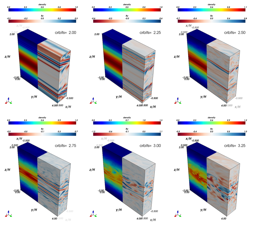
Figure 1: Snapshots during the initial phase of the MRI from Run A32a. The left and right halves in each panel show contours of the mass density and the azimuthal magnetic field, as normalized by the mid-plane density and the maximum field strength at the initial state, respectively.

3.1.1 Statistics

After 3–4 orbits pass, the simulation box is filled with chaotic turbulent motion. Statistics of various quantities are summarized in Table 2. For comparative purpose, we also show the statistics for Run I32, where all conditions are the same as in Run A32a, except for the use of isotropic pressure. The second and fourth columns from the left represent averages both in space and in time, whereas the third and fifth columns show standard deviations of volume-averaged values, which indicate the magnitude of temporal fluctuation.

From the energy distribution in Table 2, we can see that the properties of turbulent fluctuation in the two runs are quite similar. Magnetic energy, for example, is distributed into each directional component related to $B_{x}$, $B_{y}$, and $B_{z}$, respectively, roughly in the ratio of 0.1:0.85:0.05, and kinetic energy is $\sim 40\%$ of the total magnetic energy. The magnitudes of both the kinetic energy and magnetic energy, however, decrease by $\sim 20\%$ in A32a compared with the case in I32. A qualitatively similar relation also holds for stress; both Reynolds and Maxwell stresses are reduced by $\sim 20\%$ with a nearly constant ratio between them. In Run A32a, we also have additional angular-momentum transport by anisotropic stress, $p_{xy}$. The value of this anisotropic stress seems merely comparable to the contribution from the Reynolds stress. However, the 20% reduction of other stress is compensated by $p_{xy}$, and the total transport efficiency does not change significantly. The bottommost two rows in Table 2 compare the parallel and perpendicular pressures averaged over the simulation. As qualitatively predicted from the double-adiabatic approximation, in an average sense, $p_{\perp}$ dominates $p_{||}$, which causes positive $p_{xy}$ by combination with the positive Maxwell stress, because the anisotropic stress can be written as $p_{xy}\simeq\left(-B_{x}B_{y}/B^{2}\right)\left(p_{\perp}-p_{||}\right)$ when the gyrotropic assumption holds.

Table 2: Statistics for Runs A32a and I32

	A32a		I32
Quantity $f$	$\left<\left<f\right>\right>\times 10^{2}$	$\sigma_{\left<f\right>}\times 10^{2}$	$\left<\left<f\right>\right>\times 10^{2}$	$\sigma_{\left<f\right>}\times 10^{2}$
$\rho v_{x}^{2}/2p_{0}$	0.27	0.081	0.35	0.112
$\rho v_{y}^{2}/2p_{0}$	0.15	0.054	0.22	0.095
$\rho v_{z}^{2}/2p_{0}$	0.17	0.044	0.19	0.066
$B_{x}^{2}/2p_{0}$	0.12	0.057	0.19	0.091
$B_{y}^{2}/2p_{0}$	1.18	0.576	1.51	0.823
$B_{z}^{2}/2p_{0}$	0.06	0.029	0.10	0.046
$\rho v_{x}v_{y}/p_{0}$	0.14	0.050	0.17	0.068
$-B_{x}B_{y}/p_{0}$	0.47	0.181	0.60	0.239
$p_{xy}/p_{0}$	0.20	0.058	—	—
$\left(p_{||}-\left<p\right>_{t=0}\right)/p_{0}$	-0.49	0.165	—	—
$\left(p_{\perp}-\left<p\right>_{t=0}\right)/p_{0}$	0.15	0.083	—	—

Note. — Single brackets denote spatial averages over the whole simulation domain; $\sigma_{X}$ is a standard deviation for a quantity $X$.

3.1.2 Volume-averaged stress

Figure 2 shows the time histories of the volume-averaged Reynolds, Maxwell, anisotropic, and total stresses for Runs A32a and I32. Each quantity shows a highly chaotic behavior. In particular, the Maxwell stress is strongly intensified intermittently with an interval that sometimes exceeds several dozen orbits. This is the reason why considerable durations such as 300 orbits are required to obtain a temporally averaged, representative value in shearing-box simulations of MRI-driven turbulence (Winters et al., 2003).

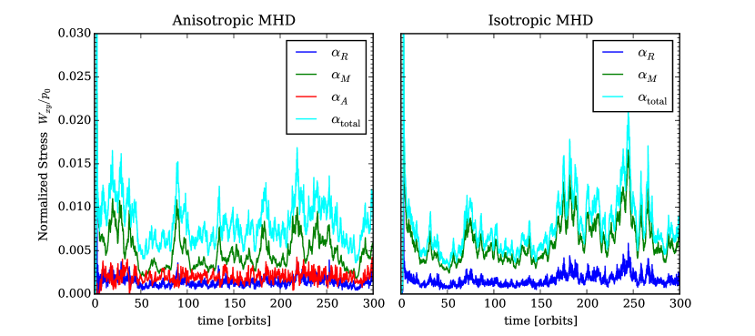
Figure 2: Time variation of $\alpha$-parameters averaged over the whole simulation domain in Runs A32a (left) and I32 (right). Contributions from the Reynolds (blue), Maxwell (green), anisotropic (red, only in the anisotropic run), and total (cyan) stresses are plotted with different colors.

Figure 3 also shows each stress averaged over the whole simulation domain after 50 orbits, but plotted as a function of the instantaneous magnetic energy. The green scattered points clearly indicate a strong correlation between the Maxwell stress and the magnetic energy. The slope of the regression line is 0.27, while the Reynolds stress shows weaker dependence with a slope of 0.054. The anisotropic stress, on the other hand, exhibits no clear dependence, with a slightly negative slope for the linear-regression line. This tendency looks quite different from that observed in an unstratified simulation (see Figure 3 in Sharma et al. (2006)). For more details, we need to see the spatial structure, which will be discussed in the next section.

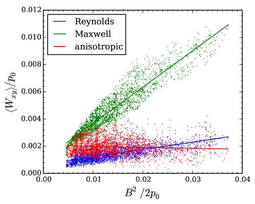
Figure 3: Dependence of each stress upon instantaneous magnetic energy. The solid lines are the results of linear fitting.

3.1.3 Vertical structure

Since the present system involves stratification, it becomes possible to study the vertical dependence of various quantities, which is a great advantage of the large-scale model. One graphical method that is helpful in understanding the vertical structure is a space-time diagram. It shows a quantity averaged along a horizontal plane as a two-dimensional function of both vertical position and time. Figures 4 and 5 compare the space-time diagrams for Runs A32a and I32, respectively. From top to bottom, we plot the color contours of the plasma beta in logarithmic scale, the radial and azimuthal magnetic flux, the Maxwell stress, and the anisotropic stress (only in A32a), each of which is properly non-dimensionalized by the initial mid-plane pressure.

From the top three panels, we can see that strongly magnetized patches generated near the disk mid-plane buoyantly rise toward the boundary regions. The magnetic flux piled up near the boundaries is apparently a spurious result of the use of periodic boundary conditions in the vertical direction. As we already mentioned, however, this structure does not affect the behavior inside the disk with $\left|z/H\right|\lesssim 1$, where the MRI is highly active. In particular, the bottom two panels show that neither the Maxwell nor the anisotropic stress has any corresponding structure near the boundaries, so the statistics of each stress in the previous section should not be significantly altered by the choice of the boundary condition. Looking at the sign of the azimuthal field in the rising patches (and also in the piled up field near the boundary), we can observe quasi-periodic reversals. This characteristic pattern is thought to be an indication of an underlying dynamo effect and has been observed commonly in previous MHD simulations in the collisional regime (e.g., Pessah et al., 2007; Vishniac, 2009; Davis et al., 2010; Gressel, 2010).

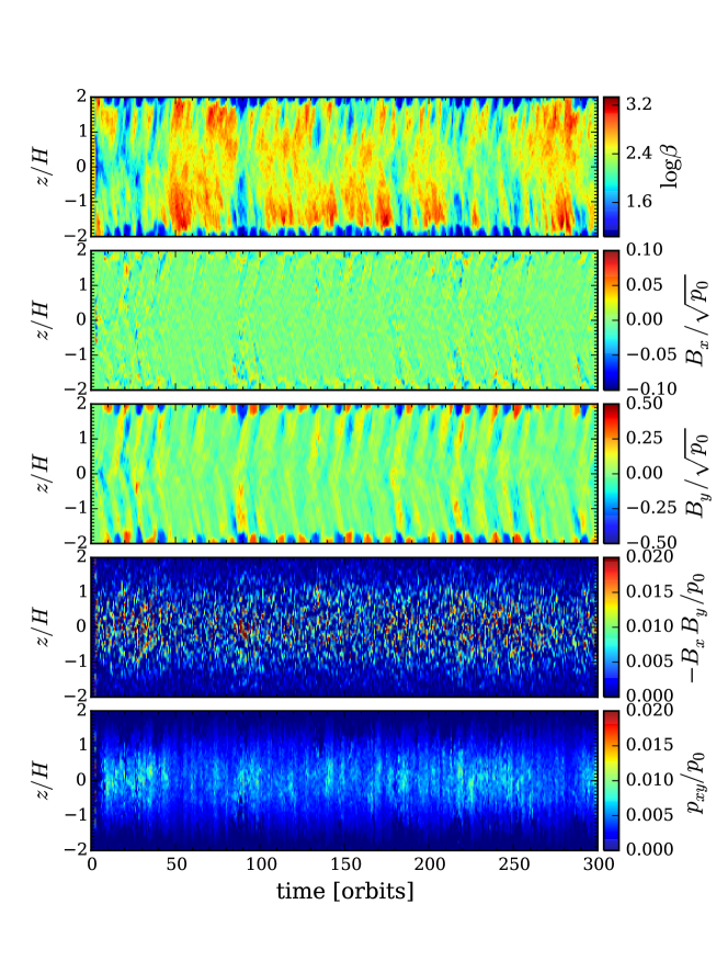
Figure 4: Horizontally averaged structure of various quantities in the anisotropic run as functions of vertical position and time in Run A32a. From top to bottom, we plot the plasma beta, the radial magnetic field, the azimuthal magnetic field, the Maxwell stress, and the anisotropic stress.

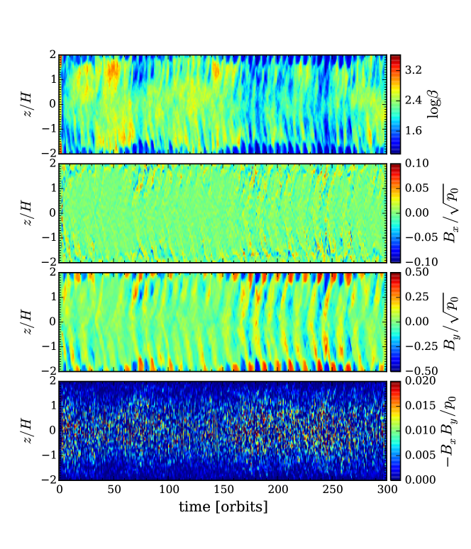
Figure 5: Space-time diagrams in isotropic Run I32 with the same format as in Figure 4.

By comparison with Run I32 shown in Figure 5, it can be said that the magnetic structure described here is qualitatively similar to that in the isotropic case. The vertical distribution of the anisotropic stress, however, is rather different from the other two components. To make this point clearer, we take a further average of time after 50 orbits, yielding the temporally and horizontally averaged, one-dimensional vertical profiles of the stress in Figure 6, where each stress is colored in the same way as in Figure 2. Again, the left and right panels represent the results for Runs A32a and I32, respectively.

It is remarkable that the anisotropic stress localizes around the disk mid-plane, although the Maxwell and Reynolds components have broader structures over a wide range of height, just as in the isotropic MHD run. As a result, the total efficiency of angular-momentum transport also has a localized profile rather than a flat, or two-peak, distribution like that obtained in I32 and previous studies (Davis et al., 2010). This localization indicates that, for angular-momentum transport in collisionless disks, the effect of the background structure of an accretion disk could be more essential than expected in collisional disks. In particular, although unstratified-shearing-box simulations have predicted a magnitude of anisotropic stress comparable to that of the Maxwell stress, our stratified model shows that it is true only at the deep inside of the disk, $\left|z/H\right|\lesssim 0.5$, and that the anisotropic stress decreases gradually but more sharply than the other stresses as $z$ moves away from the disk mid-plane. Note that it is not surprising that the results of the unstratified models agree well with the activity around the mid-plane because the vertical gravity is proportional to $z$.

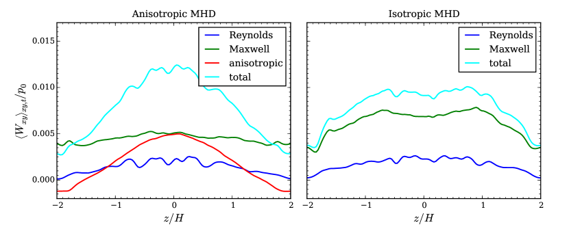
Figure 6: Comparison of the vertical structures of horizontally and temporally averaged stresses between Runs A32a and I32.

The localization of the anisotropic stress seems to be explained as follows. $\alpha_{A}$, which is a part of $\alpha$ carried by the anisotropic stress, can be written as

$$\alpha_{A}=\frac{p_{xy}}{p_{0}}\simeq\left(\frac{p_{\perp}-p_{||}}{B^{2}}\right)\left(\frac{-B_{x}B_{y}}{p_{0}}\right)=\left(\frac{\beta_{\perp}-\beta_{||}}{2}\right)\alpha_{M},$$ (13)

where $\alpha_{M}$ is the Maxwell stress normalized by $p_{0}$. This means that, even if anisotropy is somewhat uniform in the sense of $p_{\perp}/p_{||}$, $\alpha_{A}$ can vary largely depending on the magnitude of the diagonal components in the pressure tensor itself. This argument is illustrated in Figure 7. From top to bottom, plotted are the horizontally and temporally averaged profiles of the parallel and perpendicular pressure, the ratio and the difference between them, and the magnetic energy density, respectively, aer plotted within $\left|z/H\right|\leq 1.5$, where the spurious boundary effect is relatively weak. The first and second panels show that the anisotropy $p_{\perp}/p_{||}$ is rather uniform inside the disk, $\left|z/H\right|\simeq 1$, in the sense of their ratio, with the stratification maintained. The anisotropic stress, however, is determined by the difference of $p_{\perp}$ and $p_{||}$, which is plotted in the third panel, and it shows a convex profile due to the stratification. Since the magnetic energy density has a quite flat structure, as shown in the bottommost panel, the profile of anisotropic stress becomes nearly proportional to the stratified pressure. Although such a profile of the anisotropic stress might seem an apparent consequence, this is undoubtedly the first quantitative estimate of the anisotropic stress in a collisionless accretion disk including the disk scale.

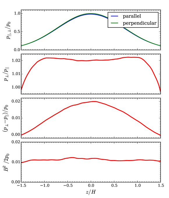
Figure 7: Horizontally and temporally averaged profiles of the variables related to anisotropic stress, $p_{xy}$.

3.2 Resolution dependence

Convergence of solutions with respect to the number of grid points is an issue of importance for numerical simulations. The grid convergence of statistics in a shearing-box model during a saturated stage of MRI has also been investigated intensively. Focusing on calculations with no net magnetic flux, it is known that the turbulent stress in cases without explicit dissipation and vertical gravity becomes smaller and smaller without bound as a higher resolution is employed (Pessah et al., 2007; Fromang & Papaloizou, 2007; Guan et al., 2009). This absence of convergence has been a long-standing mystery of shearing-box models. A resolution study using the Athena code reported in Davis et al. (2010), however, claimed that they observed convergence of the saturation amplitude of MRI-driven turbulence for resolutions up to 128 grid points per scale height, once the vertical gravity and the resultant stratification were retained. In contrast, Bodo et al. (2014) revisited the same problem with ampler computational resources using the PLUTO code, and observed no evidence of convergence with resolutions up to 200 grid points per scale height. The grid convergence of turbulent stress in a shearing-box model is still an open question.

In the case of our model as well, it is significant to assess the dependence of the transport efficiency upon the number of grid points. We list in Table 1 the results using different resolutions with 32 and 64 grid points per scale height in Runs A32a and A64 (I32 and I64 for isotropic pressure). Note that the Reynolds and Maxwell stresses in Run I64 agree remarkably well with those obtained in Run S64R1Z4 reported in Davis et al. (2010), which corresponds to the same calculation as in our Run I64. Run A64, on the other hand, shows a more sensitive increase in every component of the stress, and the total transport efficiency exceeds the isotropic case. The duration of the high-resolution run, however, is limited to only 20 orbits owing to the restriction of currently available computational resources. This duration does not seem sufficient at all for obtaining a meaningful representative value from highly chaotic turbulence, since the interval of intermittent behavior can reach several dozen orbits, as we already mentioned. We leave a more precise and robust study on convergence in simulations lasting several hundreds of orbits for future work.

3.3 Dependence on gyrotropization model

To deal with an anisotropic pressure tensor, our model introduces a timescale or a frequency to control how fast the pressure tensor approaches its gyrotropic asymptote. It is necessary to clarify the dependence of our results upon this parameter. The gyrotropization frequency enters into the system through the last term in Equation (4), where

$$\nu_{g}=\left(\frac{\left|\mathbf{B}\right|}{B_{0}}\right)\nu_{g0},$$ (14)

is set to be proportional to the local magnetic-field strength normalized by a fiducial value, $B_{0}$. In all of our calculations, $B_{0}$ is fixed at the initial maximum value of the magnetic field for $\beta=100$, i.e., $B_{0}=\sqrt{2p_{0}/10^{2}}$, which is also a typical field strength during the saturated stage. Runs A32a, A32d, and A32e in Table 1 employ different values of $\nu_{g0}$, namely, $10^{13}$, $10^{8}$ and $10^{3}$ in units of the rotation frequency of the disk, $\Omega$. These choices of $\nu_{g0}$ roughly yield $\nu_{g0}\Delta t\simeq 10^{10}$, $10^{5}$, and $1$, respectively, at a site of a typical magnetic field, using a simulation time step defined to satisfy the CFL condition. We therefore expect quantitatively similar results for Runs A32a and A32d, where $\nu_{g}\Delta t\gg 1$, and the statistics shown in Table 1 successfully demonstrate it.

Run A32e, on the other hand, shows that the Maxwell stress increased by $\sim 40\%$ whereas the Reynolds and anisotropic contributions remained unchanged. The magnetic energy is also increased by 35%. This enhancement may be traced to the reduction of released magnetic energy via magnetic reconnection under the presence of large non-gyrotropy. In HHA16, it was illustrated that eigenmodes that are not present in a gyrotropic framework can support a current sheet without resulting in an explosive reconnection event and releasing magnetically stored energy. To support this assertion, we present plots of the occurrence frequencies of non-gyrotropy in Figure 8. The vertical axis indicates a measure of non-gyrotropy, which is defined as an $L_{2}$-norm of a residue of a pressure tensor from its gyrotropic limit, as normalized by the mid-plane pressure;

$$\Delta\hat{p} \equiv \frac{1}{p_{0}}\sqrt{\sum_{i,j}\bigl{|}p_{ij}-p_{g,ij}\bigr{|}^{2}},$$

$$= \frac{1}{p_{0}}\sqrt{(p_{xx}-p_{g,xx})^{2}+(p_{xy}-p_{g,xy})^{2}+\dots+(p_{zz}-p_{g,zz})^{2}}.$$

The horizontal axis shows the magnetic-field strength on a logarithmic scale, and the number of cells counted during 50–100 orbits is shown by the color contour. From left to right, the panels show the results for Runs A32a, A32d, and A32e, respectively.

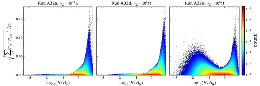
Figure 8: Occurrence frequencies of a measure of non-gyrotropy and magnetic-field strength, for Runs A32a, A32d, and A32e using different gyrotropization frequencies.

Again, the two left panels for Runs A32a and A32d show the quite similar results; a majority of data crowds around a narrow region along $\Delta\hat{p}\simeq 0$. Note that $\nu_{g}\Delta t\gg 1$ holds over the entire range field strengths in these two runs. In the rightmost panel for the smallest value of $\nu_{g0}$, however, a large non-gyrotropy with at most $\Delta\hat{p}\simeq 0.1$ remains in the weakly magnetized regions, which can be thought as sites where magnetic reconnection takes place. The extent to which this highly non-uniform non-gyrotropy alters the dynamics of reconnection is still unclear. Nevertheless, in a qualitative sense at least, our result seems consistent with the suppression of reconnection by the non-gyrotropic entropy modes as pointed out in HHA16.

The enhanced stress in Run A32e highlights the important role of deviation from gyrotropic pressure, which updates the previous result of the shearing-box simulation with the gyrotropic framework by Sharma et al. (2006). Even though the volume occupancy of weakly magnetized regions with finite non-gyrotropy is not very large, it can have a significant impact upon the full large-scale dynamics through the process of magnetic reconnection. This is a good example of the multi-scale coupling typical in collisionless plasmas, and we have suggested a new aspect of micro-physics to be taken into account in large-scale collisionless accretion disks.

3.3.1 Combined model of rotation and gyrotropization

For the purpose of showing one of the possible directions for improvement of the gyrotropization model, we have attempted numerical experiments to include the effect of rotation of a pressure tensor in addition to gyrotropization; we solve

$$\frac{\partial p_{ij}}{\partial t}=\Omega_{c}\left(\varepsilon_{ikl}p_{jk}\hat{b}_{l}+\varepsilon_{jkl}p_{ik}\hat{b}_{l}\right)-\nu_{g}\left(p_{ij}-p_{g,ij}\right),$$

instead of only the gyrotropization effect, whose right-hand side includes only the last term with $\nu_{g}$. This is motivated by the fact that the original form of this operator simply describes the rotation of a pressure tensor by cyclotron motion of particles (see Equation (12) in HHA16). By solving this term analytically in an operator-splitting manner, the effect that a particle incoming into a neutral sheet quickly changes its direction of cyclotron motion, which is one of the essential phenomena in magnetic reconnection, may be incorporated into the system. In practice, since our model employs a one-fluid framework, we have to determine the direction in which particles rotate. In the present application, suppose that the pressure is mainly supported by ions and a positive value is adopted for $\Omega_{c}$, which is defined in the same way as $\nu_{g}$;

$$\Omega_{c}=\left(\frac{\left|\mathbf{B}\right|}{B_{0}}\right)\Omega_{c0}.$$

The role of this rotation term, particularly on magnetic reconnection, is discussed in Appendix B using a one-dimensional Riemann problem that imitates the self-similar Petschek-type reconnection layer, and we find that the fast rotation of a pressure tensor around a local magnetic-field line behaves in a qualitatively similar way to the previous model, whereas gyrotropization is not guaranteed explicitly. In spite of the similarity, inclusion of this original rotation term still has an advantage. We observed that, when applied to stratified-disk simulations, it becomes possible to employ smaller $\nu_{g0}$ than listed in Table 1 for the first time by using the combined model; otherwise, the simulation with, for example, $\nu_{g0}=10\Omega$ breaks down owing to the appearance of negative density. On the contrary, a merit of incorporating with the gyrotropization model is to guarantee consistency with the gyrotropic limit in an asymptotic manner by reducing non-gyrotropy explicitly.

3.3.2 Application to stratified-disk simulations

In this section, let us apply the combined model introduced above to our stratified-disk model. For simplicity, we assume $\Omega_{c0}=\nu_{g0}$ here. The simulation parameters and the resultant stress averaged both in space and time are summarized in Table 3 with the same format as in Table 1. Each run is labeled with R (with rotation). From Run R32a to Run R32d, the frequency common to the gyrotropization and rotation procedures is changed.

Table 3: Simulation summary for the rotation + gyrotropization model

Run	Resolution	Orbits	$\beta$	$\nu_{g0}/\Omega$	$\left<\left<\rho v_{x}v_{y}\right>\right>/p_{0}$	$\left<\left<-B_{x}B_{y}\right>\right>/p_{0}$	$\left<\left<p_{xy}\right>\right>/p_{0}$
R32a	$32/H$	300	$10^{2}$	$10^{13}$	0.0014	0.0045	0.0019
R32b	$32/H$	300	$10^{2}$	$10^{8}$	0.0015	0.0048	0.0020
R32c	$32/H$	300	$10^{2}$	$10^{3}$	0.0016	0.0057	0.0021
R32d	$32/H$	300	$10^{2}$	$10^{1}$	0.0019	0.0121	0.0090

The dependence of the stress on $\nu_{g0}$ is illustrated in Figure 9 along with the averaged plasma beta. The A32 and R32 series are represented by circles and squares, respectively. We can clearly see that both series are in qualitative and quantitative agreement for $\nu_{g0}\gtrsim 10^{3}\Omega$, which ensures that the current model is an appropriate extension of the original model when a pressure tensor is well gyrotropized. The intensive enhancement in the Maxwell and anisotropic stresses is, however, observed when $\nu_{g0}$ is further decreased to $10\Omega$ in Run R32d, and the magnetic energy is also roughly tripled compared with the case of $\nu_{g0}=10^{3}\Omega$. Although these facts seem to imply a more efficient dynamical suppression of magnetic reconnection by a non-gyrotropic pressure, the increase not only in the Maxwell stress but also in the anisotropic stress may be related to a process slightly different from the case in A32e or R32c. For example, it is known in the kinetic description that charged particles entering a reconnection layer experience Speiser orbits toward the direction of the electric field along an X-line. The particular situation in a shearing box is illustrated in Figure 10. Since the magnetic field is continuously stretched in the $x$-direction by the MRI and in the $y$-direction by background differential rotation, reconnection is expected to occur in a plane inclined from both the $\left(x,z\right)$- and $\left(y,z\right)$-planes, like the shaded region. Thus, the population in Speiser orbits tends to have a correlation of $\left<v_{x}v_{y}\right>>0$, which contributes to positive $p_{xy}$ in quite non-gyrotropic manner. Getting back to our fluid model, although each particle’s orbit is not resolved, it may be possible to generate this non-gyrotropic $p_{xy}$ by distorting and rotating the pressure of incoming flux with large $p_{\perp}$. This effect cannot be captured when only gyrotropization is assumed, where the anisotropy around the magnetic field remains in a constant direction. Demonstrating this hypothesis, however, requires a more detailed study of magnetic reconnection itself in an isolated system. In any case, the result here emphasizes the striking dependence of the angular-momentum-transport efficiency upon the ratio between the cyclotron frequency and the disk’s rotation frequency. Note that, since the previous PIC simulations by Hoshino (2015) assumed a small ratio, $\Omega_{c}/\Omega=10$, to save computational resources, it may be possible to overestimate the suppression effect due to the non-gyrotropic distribution function. It is to be hoped that future research will clarify this point.

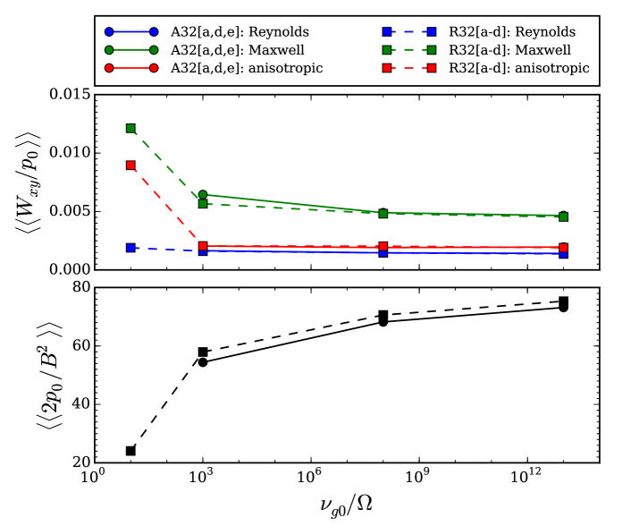
Figure 9: Dependence of stress and plasma beta upon the gyrotropization and cyclotron frequency. The circles connected with solid lines are the cases with only gyrotropization, and the squares connected with dashed lines indicate the result of the gyrotropization and rotation model.

Figure 10: A schematic diagram of a reconnection layer expected in a shearing-box simulation.

4 Discussion and summary

In this paper, we have conducted a series of stratified-shearing-box simulations in the collisionless regime using the recently developed kinetic-MHD model, which can handle finite deviation from the gyrotropic pressure. This is the first approach to the large-scale dynamics of collisionless accretion disks. In particular, it is designed to bridge the gap between double-adiabatic simulations assuming gyrotropic pressure and fully kinetic simulations, which cannot handle disk scales.

The main results of importance are summarized as follows:

1. The volume- and time-averaged total efficiency of angular-momentum transport remains at the same level as in isotropic MHD simulations for large gyrotropization rates.

2. The distribution ratio of the Reynolds, Maxwell, and anisotropic stresses agrees with unstratified simulations only near the disk’s mid-plane, and anisotropic stress decreases outwardly.

3. The results are not affected by the choice of the artificial parameter used to determine the gyrotropization rate, as long as it is sufficiently large.

4. Once the gyrotropization rate approaches the dynamical timescale of the disk, finite non-gyrotropy around neutral sheets tends to enhance the Maxwell stress.

Although the result 1 looks the same as the argument claimed in a previous study of unstratified simulations using the double-adiabatic model (Sharma et al., 2006), the contribution from the anisotropic stress is only comparable to the Reynolds stress, rather than to the Maxwell stress as predicted in the unstratified case. The properties of the unstratified-shearing-box model are well reproduced only around the disk’s mid-plane, where the effect of vertical gravity is weak and stratification can be ignored to a good approximation. The stratified pressure, however, yields the strong dependence of the anisotropic stress upon the vertical position. Specifically, as stated in result 2, the anisotropic stress decreases outwardly away from the mid-plane, reflecting stratification of the diagonal pressure, whereas the Maxwell and Reynolds stresses have broader distributions. This fact apparently suggests that the large-scale structure is more essential for angular-momentum transport in a collisionless accretion disk than expected in a collisional disk where thermal pressure cannot carry angular momentum. Our results represent an important foothold for a deeper understanding of the global behavior of collisionless disks in the future.

A self-similar solution for Sgr A* based on the ADAF model (Narayan & Yi, 1994) predicts that the ratio of the cyclotron frequency to the rotational frequency of the disk largely depends upon an orbital radius, but is, in general, expected to be much greater than unity. Result 3 relieves us of a distress about a practical choice for a gyrotropization frequency. When it is artificially set to a value comparable to a dynamical frequency, on the other hand, the energy released through magnetic reconnection could be suppressed by finite non-gyrotropy, and an efficient transport is likely to be sustained by the increased Maxwell stress. Result 4 is qualitatively consistent with PIC simulations in Hoshino (2015), though we must note that the physics suppressing the reconnection process would be quite different. It is a highly challenging matter of interest to improve our current model to capture this suppression effect, which is believed to reflect micro-physics in part, and a large gyrotropization rate is maintained outside of the current sheets, where macro-physics plays a role. Note that the role of non-gyrotropy in the context of MRIs was not discussed in fully kinetic PIC simulations by Hoshino (2015), where suppression of magnetic reconnection and the resultant enhancement of angular-momentum transport were accounted for only in terms of gyrotropic anisotropy with $p_{||}>p_{\perp}$. Although there have been theoretical and numerical studies on non-gyrotropic electron pressure, which strongly affects the physics of resistivity, and hence magnetic reconnection, through the generalized Ohm’s law (e.g., Hesse & Winske, 1993, 1994; Yin & Winske, 2003), its dynamical role has not been discussed with interest. The simple test problem of mimicking a one-dimensional reconnection layer and its indirect application to a larger system demonstrated here emphasizes the necessity of seeing the importance of the non-gyrotropic components of a pressure tensor in a new light.

It should be noted that our model currently does not include the effect of resistivity, which is another large issue for determining the saturation amplitudes of MRI-driven turbulence. The lack of resistivity is due to the distribution of thermal energy generated by Joule heating of each component of a pressure tensor that cannot be determined within the fluid framework. This means that magnetic reconnection occurs only through numerical dissipation in the current model, and the heating rate of each component of a pressure tensor is not under control. We, however, could employ a model of the heating rates, for example, based on the idea that the Joule heating is mainly carried by electrons that isotropize instantaneously. Conversely, it is possible to construct a model of anisotropic heating of ions. Investigating the dependence of the present results upon resistivity models is also left as future work to be discussed.

Appendix A Orbital-Advection Scheme with Anisotropic Pressure

The orbital-advection scheme introduced in Stone & Gardiner (2010) is a numerical technique to integrate MHD equations in a shearing box accurately and efficiently by decomposing the system into two subsystems; one is a simple linear system which describes advection by background-differential rotation, and the other is a standard hyperbolic system with modified shearing-source terms. Since a detailed numerical implementation is provided in Stone & Gardiner (2010), here, we only reproduce the practical equations employed in our simulation code for the sake of completeness, along with comments on a few modifications required to apply the orbital-advection scheme to the kinetic-MHD model with an anisotropic-pressure tensor.

Let us decompose Equations (1)–(4). The subsystem for linear advection can be written simply as follows:

$$\frac{\partial\rho}{\partial t}+v_{K}\frac{\partial\rho}{\partial y}=0,$$ (A1)

$$\frac{\partial\rho\mathbf{v}^{\prime}}{\partial t}+v_{K}\frac{\partial\rho\mathbf{v}^{\prime}}{\partial y}=0,$$ (A2)

$$\frac{\partial\mathbf{B}}{\partial t}-\nabla\times\left(v_{K}\hat{\mathbf{e}}_{y}\times\mathbf{B}\right)=0,$$ (A3)

$$\frac{\partial\mathbf{E}^{\prime}}{\partial t}+v_{K}\frac{\partial\mathbf{E}^{\prime}}{\partial y}=\mathbf{s}_{E^{\prime}},$$ (A4)

where $v_{K}=-q\Omega x$ represents the background Keplerian velocity, $\mathbf{v}^{\prime}=\mathbf{v}-v_{K}\hat{\mathbf{e}}_{y}$ is the deviation from the Keplerian rotation, $\mathbf{E}^{\prime}=\rho\mathbf{v}^{\prime}\mathbf{v}^{\prime}+\mathbf{p}+\mathbf{BB}$ is a generalized energy tensor, and

$$\mathbf{s}_{E^{\prime}}=-\left(\rho v_{x}^{\prime}v_{y}^{\prime}+p_{xy}-B_{x}B_{y}\right)\frac{dv_{K}}{dx}\left(\begin{array}[]{ccc}0&1&0\\ 1&2&1\\ 0&1&0\\ \end{array}\right).$$ (A8)

Since the advection velocity is purely along the $y$-axis and constant in time, these equations can be integrated using their analytical solutions without constraint upon the CFL condition. In practice, this procedure is implemented in a similar way to the shearing periodic boundary condition, although we must take special care of the divergence-free condition for a magnetic field. The right-hand side of Equation (A4) cannot be gathered up in a flux form and is treated as a source term separately.

By subtracting Equations (A1)–(A4) from Equations (1)–(4), we find that the remaining part yields the following subsystem:

$$\frac{\partial\rho}{\partial t}+\nabla\cdot\left(\rho\mathbf{v}^{\prime}\right)=0,$$ (A9)

$$\frac{\partial\rho\mathbf{v}^{\prime}}{\partial t}+\nabla\cdot\left(\rho\mathbf{v}^{\prime}\mathbf{v}^{\prime}+\mathbf{p}+\frac{B^{2}}{2}\mathbf{I}-\mathbf{BB}\right)=2\rho\Omega v_{y}^{\prime}\hat{\mathbf{e}}_{x}+\left(q-2\right)\rho\Omega v_{x}^{\prime}\hat{\mathbf{e}}_{y}-\rho\Omega^{2}z\hat{\mathbf{e}}_{z},$$ (A10)

$$\frac{\partial\mathbf{B}}{\partial t}-\nabla\times\left(\mathbf{v}^{\prime}\times\mathbf{B}\right)=0,$$ (A11)

$$\partial_{t}E_{ij}^{\prime}+\partial_{k}\left(\rho v_{i}^{\prime}v_{j}^{\prime}v_{k}^{\prime}+p_{ij}v_{k}^{\prime}+p_{ik}v_{j}^{\prime}+p_{jk}v_{i}^{\prime}+\mathcal{S}_{kij}^{\prime}+\mathcal{S}_{kji}^{\prime}\right)$$

$$=B_{i}v_{k}^{\prime}\partial_{k}B_{j}+B_{j}v_{k}^{\prime}\partial_{k}B_{i}-B_{k}v_{i}^{\prime}\partial_{j}B_{k}-B_{k}v_{j}^{\prime}\partial_{i}B_{k}$$

$$+v_{i}^{\prime}s_{g,j}^{\prime}+v_{j}^{\prime}s_{g,i}^{\prime}-\nu_{g}\left(p_{ij}-p_{g,ij}\right),$$ (A12)

where quantities with primes are evaluated using $\mathbf{v}^{\prime}$ rather than $\mathbf{v}$ itself, and

$$\mathbf{s}_{g}^{\prime}=\left(\begin{array}[]{c}2\rho\Omega v_{x}^{\prime}\\ -2\rho\Omega v_{y}^{\prime}\\ -\rho\Omega^{2}z\end{array}\right).$$ (A16)

The gravitational and Coriolis forces are slightly modified from the original shearing box system. These equations are integrated in a standard manner. Note that Equations (A4) and (A12) are reduced to Equations (51) and (55) in Stone & Gardiner (2010), respectively, by taking their trace.

Appendix B One-dimensional Riemann problem with the rotation term

In order to clarify the role of the rotation term introduced in Section 3.3.1, particularly on magnetic reconnection, let us reconsider the same one-dimensional Riemann problem as described in HHA16 by setting $\Omega_{c}=\left(B/B_{0}\right)\Omega_{c0}$ and $\nu_{g0}=0$. Here we briefly reproduce the initial setup. Let us consider a Harris-type current sheet at rest threaded by a uniform guide field and focus upon the one-dimensional cross section across the current sheet, which is taken as the $x$-direction. Then, the initial magnetic field is as follows:

$$\mathbf{B}\left(x,t=0\right)=B_{0}\cos\phi\tanh\left(x/L\right)\hat{\mathbf{e}}_{y}+B_{0}\sin\phi\ \hat{\mathbf{e}}_{z},$$ (B1)

where $B_{0}$ is the magnetic-field strength in the lobe regions, $L$ is the half width of the initial sheet, and $\phi$ is fixed to $30^{\circ}$. The density and the isotropic thermal pressure are distributed so as to maintain thermal and dynamical equilibrium, respectively. Finally, reconnected flux $B_{n}=5\times 10^{-2}B_{0}$ is added in the $x$-direction, which triggers Petschek-type reconnection.

The snapshots adopting different values of the rotation frequency, i.e., $\Omega_{c0}L/V_{A}=10^{0}$, $10^{-2}$, and $10^{-4}$ are shown in Figures 11 to 13, respectively. By comparison between Figures 5 in HHA16 and Figure 11, it is remarkable that when $\Omega_{c0}^{-1}$ takes the same order as the Alfvén transit time across the initial current sheet, the resultant structure of the reconnection layer is almost the same as that observed under the gyrotropic limit in spite of the absence of any explicit gyrotropization term. The resemblance to the gyrotropic case can be traced to redistribution of non-gyrotropic components generated at a certain gyrophase into a wide range of gyrophases. Fast rotation, therefore, tends to randomize non-gyrotropy, which effectively works like gyrotropization, although it is not guaranteed that non-gyrotropy vanishes eventually. The only major difference from the gyrotropic limit is the behavior of the rotational discontinuities around $\left|x/L\right|\sim 90$, where the responses of various quantities are anti-symmetric between leftward- and rightward-propagating waves. This symmetry breaking apparently arises from the assumption that the pressure is supported only by positive charges, i.e., $\Omega_{c}>0$, and thus reflects the direction of the local magnetic field.

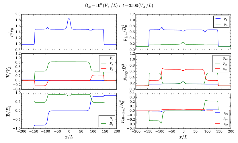
Figure 11: Results of the one-dimensional Riemann problem at $t=3,500$ including only the rotation term with $\Omega_{c0}=10^{0}$.

When the rotation is slower than the dynamical timescale, as shown in Figure 12 with $\Omega_{c0}=10^{-2}V_{A}/L$, the reconnection layer becomes quite complicated and highly asymmetric. It is no longer straightforward to understand the structure based on the propagation of isolated waves. Once the rotation frequency is further decreased by two orders of magnitude, however, the system shows no explosive reconnection, as shown in Figure 13. This naturally occurs under the same mechanism described in HHA16 and Figure 6 there, and the assumption of positive $\Omega_{c}$ causes a slight leftward migration of the contact discontinuity.

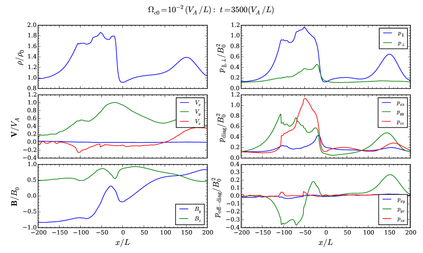
Figure 12: Results of the one-dimensional Riemann problem at $t=3,500$ including only the rotation term with $\Omega_{c0}=10^{-2}$.

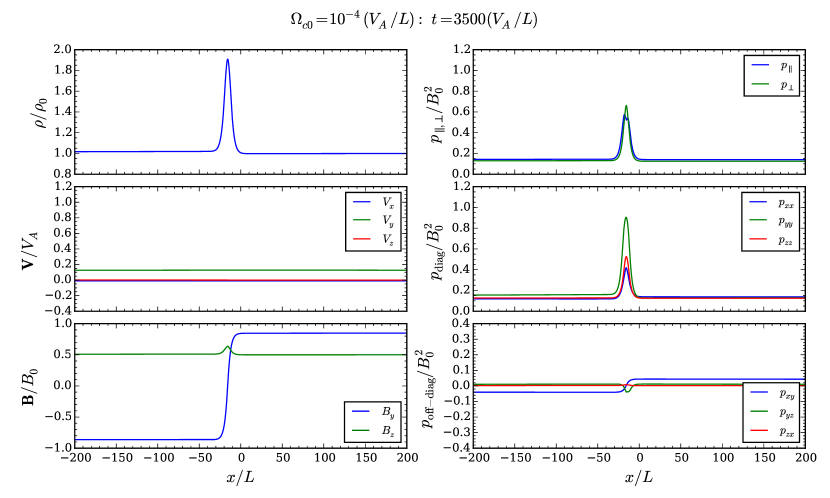
Figure 13: Results of the one-dimensional Riemann problem at $t=3,500$ including only the rotation term with $\Omega_{c0}=10^{-4}$.

References

- Balbus & Hawley (1991) Balbus, S. A., & Hawley, J. F. 1991, ApJ, 376, 214
- Birn & Hesse (2001) Birn, J., & Hesse, M. 2001, J. Geophys. Res., 106, 3737
- Bodo et al. (2014) Bodo, G., Cattaneo, F., Mignone, A., & Rossi, P. 2014, ApJ, 787, L13
- Brandenburg et al. (1995) Brandenburg, A., Nordlund, A., Stein, R. F., & Torkelsson, U. 1995, ApJ, 446, 741
- Chen & Palmadesso (1984) Chen, J., & Palmadesso, P. 1984, Physics of Fluids, 27, 1198
- Chew et al. (1956) Chew, G. F., Goldberger, M. L., & Low, F. E. 1956, Proceedings of the Royal Society of London Series A, 236, 112
- Davis et al. (2010) Davis, S. W., Stone, J. M., & Pessah, M. E. 2010, ApJ, 713, 52
- Doeleman et al. (2008) Doeleman, S. S., Weintroub, J., Rogers, A. E. E., et al. 2008, Nature, 455, 78
- Falcke & Markoff (2000) Falcke, H., & Markoff, S. 2000, A&A, 362, 113
- Fromang & Papaloizou (2007) Fromang, S., & Papaloizou, J. 2007, A&A, 476, 1113
- Gressel (2010) Gressel, O. 2010, MNRAS, 405, 41
- Guan et al. (2009) Guan, X., Gammie, C. F., Simon, J. B., & Johnson, B. M. 2009, ApJ, 694, 1010
- Hammett & Perkins (1990) Hammett, G. W., & Perkins, F. W. 1990, Physical Review Letters, 64, 3019
- Hau & Wang (2016) Hau, L.-N., & Wang, B.-J. 2016, Journal of Geophysical Research (Space Physics), 121, 6245
- Hawley et al. (1995) Hawley, J. F., Gammie, C. F., & Balbus, S. A. 1995, ApJ, 440, 742
- Hesse & Winske (1993) Hesse, M., & Winske, D. 1993, Geophys. Res. Lett., 20, 1207
- Hesse & Winske (1994) —. 1994, J. Geophys. Res., 99, 11177
- Hirabayashi et al. (2016) Hirabayashi, K., Hoshino, M., & Amano, T. 2016, Journal of Computational Physics, 327, 851
- Hoshino (2015) Hoshino, M. 2015, Physical Review Letters, 114, 061101
- Johansen et al. (2009) Johansen, A., Youdin, A., & Klahr, H. 2009, ApJ, 697, 1269
- Kusunose & Takahara (2012) Kusunose, M., & Takahara, F. 2012, ApJ, 748, 34
- Miller & Stone (2000) Miller, K. A., & Stone, J. M. 2000, ApJ, 534, 398
- Narayan & Yi (1994) Narayan, R., & Yi, I. 1994, The Astrophysical Journal, 428, L13
- Narayan et al. (1995) Narayan, R., Yi, I., & Mahadevan, R. 1995, Nature, 374, 623
- Pessah et al. (2006) Pessah, M. E., Chan, C.-K., & Psaltis, D. 2006, MNRAS, 372, 183
- Pessah et al. (2007) Pessah, M. E., Chan, C.-k., & Psaltis, D. 2007, ApJ, 668, L51
- Shakura & Sunyaev (1973) Shakura, N. I., & Sunyaev, R. A. 1973, A&A, 24, 337
- Sharma et al. (2006) Sharma, P., Hammett, G. W., Quataert, E., & Stone, J. M. 2006, The Astrophysical Journal, 637, 952
- Stone & Gardiner (2010) Stone, J. M., & Gardiner, T. A. 2010, The Astrophysical Journal Supplement Series, 189, 142
- Stone et al. (1996) Stone, J. M., Hawley, J. F., Gammie, C. F., & Balbus, S. A. 1996, ApJ, 463, 656
- Suzuki & Inutsuka (2009) Suzuki, T. K., & Inutsuka, S.-i. 2009, ApJ, 691, L49
- Vishniac (2009) Vishniac, E. T. 2009, ApJ, 696, 1021
- Winters et al. (2003) Winters, W. F., Balbus, S. A., & Hawley, J. F. 2003, MNRAS, 340, 519
- Yin & Winske (2003) Yin, L., & Winske, D. 2003, Physics of Plasmas, 10, 1595