MSUHEP-17-006
Variance Reduction and Cluster Decomposition
Abstract
It is a common problem in lattice QCD calculation of the mass of the hadron with an annihilation channel that the signal falls off in time while the noise remains constant. In addition, the disconnected insertion calculation of the three-point function and the calculation of the neutron electric dipole moment with the term suffer from a noise problem due to the fluctuation. We identify these problems to have the same origin and the problem can be overcome by utilizing the cluster decomposition principle. We demonstrate this by considering the calculations of the glueball mass, the strangeness content in the nucleon, and the CP violation angle in the nucleon due to the term. It is found that for lattices with physical sizes of 4.5 - 5.5 fm, the statistical errors of these quantities can be reduced by a factor of 3 to 4. The systematic errors can be estimated from the Akaike information criterion. For the strangeness content, we find that the systematic error is of the same size as that of the statistical one when the cluster decomposition principle is utilized. This results in a 2 to 3 times reduction in the overall error.
I Introduction
As the physical pion mass is accessible in lattice QCD simulations nowadays with larger physical volumes and several lattice spacings with different lattice actions to estimate the associated systematic errors, lattice QCD calculation is getting mature, particularly for flavor physics where the quark masses, heavy-light decay constants, CKM matrices, and strong coupling constant are reviewed and averaged by FLAG Aoki et al. (2017). On the other hand, the baryon physics is not as settled as that of mesons. Part of the reasons is illustrated in the Parisi-Lepage consideration of the signal-to-noise ratio of the nucleon two-point function. Since the variance of the nucleon propagator has three-pions as the lowest state in the correlator, the signal-to-noise (S/N) ratio is proportional to Parisi (1984); Lepage (1989) and noticeably grows exponentially with when the pion mass is close to the physical one in lattice calculations. This is why baryon physics is more noisy than that of mesons.
One special problem associated with the correlators of mesons involving annihilation channels or glueballs is that the signal falls off exponential with time, but the noise remains constant. Thus, after certain time separation, the signal falls below the noise and succumbs to the sign problem. Another aspect of the DI is observed in the DI three-point function involving a quark loop or the topological charge in the neutron electric dipole moment (nEDM) calculation from the term, the fluctuations of the quark loop and the topological charge are proportion to which pose a challenge for calculations large volumes lattices. In this work, we shall show that the constant error and fluctuation in the DI have the same origin and they can be ameliorated with the help of the property of the cluster decomposition principle so that the S/N ratio can be improved by a factor of where is the volume with radius which is the effective correlation length between the operators.
II Cluster decomposition principle and variance reduction
One often invokes the locality argument to justify that experiments conducted on Earth is not affected by events on the Moon. This is a consequence of the cluster decomposition principle (CDP) in that if color-singlet operators in a correlator are separated by a large enough space-like distance, the correlator will be zero. In other words, the operators are not correlated in this circumstance. To be specific, it is shown Araki et al. (1962) that under the assumptions of translation invariance, stability of the vacuum, existence of a lowest non-zero mass and local commutativity, one has
| (1) |
for a large enough space-like distance , where is the vacuum-subtracted correlation function. and are two color-singlet operator clusters whose centers are at and respectively, is the smallest non-zero mass for the correlator, and is a constant. This is the asymptotic behavior of a boson propagator . This means the correlation between two operator clusters far apart with large enough space-like distance tends to be zero at least as fast as . Given that the longest correlation length in QCD is , one has . Since the Euclidean separation is always ‘space-like’, the cluster decomposition principle (CDP) is applicable to the Euclidean correlators. Some of the recent attempts to reduce variances in the calculations of strangeness in the nucleon Bali et al. (2009), the meson mass Chen et al. (2015), the light-by-light contribution in the muonic Blum et al. (2016a), the factorization of fermion determinant Cè et al. (2017), and reweighting of nEDM calculation with topological charge density Shintani et al. (2016) have applied concepts similar or related to that of CDP. In this work, we prove that, applying the CDP explicitly, the error of an DI correlator can be improved by a factor of .
In evaluating the correlators, one often takes a volume sum over the three-dimensional coordinates. To estimate at what distance the large distance behavior saturates, we integrate the fall-off to a cut off distance ,
| (2) |
where is the error function. Since the kernel of the integral decays very quickly, the integral has already gained more than of its total value for . Assuming the fall-off behavior dominates the volume-integrated correlator, we consider as an effective cutoff and the correlation with separation has negligible contribution.
To test the principle of cluster decomposition with lattice data, we consider the two-point correlator for a fixed with a cutoff of in the relative coordinate between the two color-singlet operators and
| (3) |
where . The correlation functions in the present work are calculated using valence overlap fermions on the RBC-UKQCD flavor domain-wall configurations. More detailed definitions and numerical implementations can be found in previous works Li et al. (2010); Gong et al. (2013); Sufian et al. (2017); Yang et al. (2016a).
We examine the nucleon two-point function first on the lattice (48I) with the physical sea quark mass Blum et al. (2016b). We use 3 valence quark masses corresponding to pion masses MeV, MeV and MeV respectively.
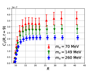
The results for the nucleon correlators at for three different valence quark masses are plotted in Fig. 1 as a function of which is the cutoff of the Euclidean distance between the point source and the sink. We see that the nucleon correlator basically saturates after fm with fm for the three cases. This agrees well with our earlier estimate of a saturation radius which corresponds to fm. This shows that the CDP works and Eq. (2) gives a good estimate of .
Since the signal of the correlators falls off exponentially with , summing over beyond the saturating radius does not change the signal and will only gather noise. Let’s consider the disconnected insertion next and see how the S/N ratio can be improved with this observation. In the case of the DI, the variance of the correlator in Eq. (3) can have a vacuum insertion in addition to the exponential fall off in due to the operator.
| (4) | |||||
where and respectively. For the case where and are integrated over the whole lattice volume, the sum over the positions and can be carried out independently. Consequently, and in the DI fluctuate independently which leads to a variance which is the product of their respective variances. In this case, the leading vacuum insertion is a constant, independent of . This is the reason why the noise remains constant over in DI. On the other hand, the constant variance is reduced to when it is integrated to , while the signal is not compromised. The sub-leading contribution (denoted by …) in Eq. (4) has an exponential decay in with a mass in the scalar channel. It is clear that to leading order, the ratio of the cutoff S/N at to that without cutoff is
| (5) |
We shall consider several DI examples involving volume summations over two or more coordinates. Since the convoluted sum with a relative coordinate in Eq. (3) can be expensive, we shall invoke the standard convolution theorem by calculating the product of two functions where is the Fourier transforms of in each configuration on their respective time slices. Then
| (6) |
where is the Fourier transform of . In this way, the cost of the double-summation, which is order , is reduced to that of the fast Fourier transform (FFT) which is in the order of .
II.1 Scalar matrix element of the strange quark
The first example is the disconnected insertion for the nucleon matrix element with a scalar loop which involves a three-point function and can be expressed as
| (7) |
where is the vacuum-subtracted scalar loop, denotes the source grid for increasing statistics Li et al. (2010). Note here is the 4-D distance and is the spatial separation between the loop and the sink. Since the low-modes dominate the strangeness in the nucleon Yang et al. (2016b), we calculate the strange quark loop with low-modes only to illustrate the CDP effect. The sum over the spatial relative coordinate between the scalar quark loop and the sink interpolation operator is carried out through the convolution in Eq. (6). This calculation is done on the domain-wall (32ID) lattice Blum et al. (2016b) with pion mass MeV and the lattice size is fm.
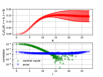
The upper panel of Fig. 2 gives the value and the error of the ratio of three-to-two point functions in Eq. (7) as a function of at and . The nucleon source-sink separation is fm in this case. We see the error grows after is greater than while the central value remains constant within errors. This behavior reflects the fact that the signal without summing over falls off exponentially with , while the error remains constant as shown in the lower panel.
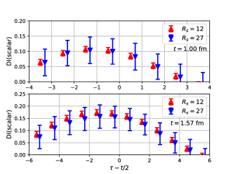
Fig. 3 shows – the disconnected three-point to two-point function ratio to obtain the scalar matrix element for the strange quark in the nucleon as a function of for two source-sink separations at 1.00 fm (upper panel) and 1.57 fm (lower panel). Two results with cutoffs of and are plotted. is the cutoff radius for the relative coordinate between the sink and the quark loop in the spatial sum. It can be seen that the central values of the two cutoffs are all consistent within errors, while the errors with cutoff are smaller than the ones with cutoff , which includes the whole spatial volume, by a factor of 4 or so. Thus, cutting off the spatial sum at the saturation distance is equivalent to gaining times more statistics.
II.2 Glueball mass
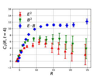
Next, we consider the glueball correlators in Eq. (3) on the 48I lattice with fm. The correlators from the scalar and operators and the pseudoscalar operator are presented in Fig. 4, where they are plotted as a function of in Eq. (3) at . We note the scalar correlators saturate after and the pseudo scalar one saturates after , which can be understood in terms of the different ground state masses in these two channels. Again, comparing the error at to that at , the latter includes the whole spatial volume, for the scalar case, the error is reduced by a factor of which is in reasonable agreement with the prediction of from Eq. (5). For the pseudoscalar case, the improvement is around 3 times and is consistent with the estimate of .
II.3 Neutron electric dipole moment:
Finally, we examine the CP-violation phase on the same 48I lattice which is needed for calculating the neutron electric dipole moment (nEDM). The phase is defined as
| (8) |
for large enough , where is the common nucleon two-point function, is the parity projector, is the nucleon propagator weighted with the total topological charge
| (9) |
We can turn the total topological charge into the summation of its density, i.e. where we use the plaquette definition for . Then the expression of with a cutoff can be cast in the same form as in Eq. (7), except the scalar quark quark loop is replaced with the local topological charge and the sum of the topological charge density is over the four sphere with a radius .
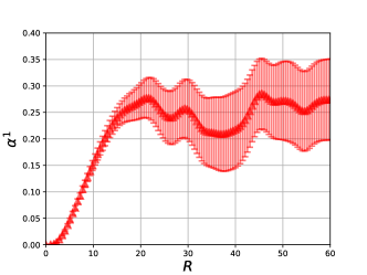
The result of as a function of in Fig. 5 shows that the signal saturates after . Cutting off the sum of at this R leads to a factor of times reduction in error compared to the case of reweighting with the total topological charge as in Eq. (9). This example indicates that for four-dimensional sums, our new method employing the CDP can also improve the S/N. As we illustrated in the introduction, the nEDM from the term suffers from a problem. It is shown here it is related to the vacuum insertion in the variance. This problem is resolved by turning the topological charge into a 4-D sum of the local charge density and applying the CDP by cutting off the relative 4-D distance in the sum.
III Systematic and statistical errors
So far, we have taken a simple cutoff to illustrate the efficacy of the variance reduction. This ad hoc choice inevitably incurs a systematic error. Since the asymptotic behavior of the integral of the correlator as a function of the separation is similar to that of the effective mass, we fit it as such and apply the Akaike information criterion (AIC) Akaike (1974) to obtain the statistical error and the estimated systematic error by using analysis with different fitting windows and models. The details of the application of AIC to the strange matrix element is provided in the Appendix as an example. It turns out that both the systematic and statistical errors are stable against multiple choices of windows and two fitting models. The statistical error is close to that at the cutoff distance when the plateau emerges (i.e. ). Using a representative fit with 2 fitting formulas and 80 combinations of 8 data points each for a total of 160 fits and 100 bootstrap samplings, we obtain the value of the strange matrix element that we considered earlier to be 0.160 (15) (15). The statistical error (first one) and the systematic error (second one) are practically the same. This is to be compared with the original value of 0.143(45) without taking the CDP into account. The systematic error is to be added to the total systematic error of the calculation.
IV Discussion and summary
Regarding the nucleon correlator in Fig. 1, we notice that there is no conspicuous increase of the error as a function of . This is because, unlike the DI, the variance does not have an vacuum insertion for the CI. The leading contribution to the variance is expected to be . This has a longer range than that of the signal which falls off with the nucleon mass. Therefore, in principle, one would expect some gain in the S/N when is cut off at . Therefore, the corresponding ratio of S/N in Eq. (5) is
| (10) |
For the 48I lattice in Fig. 1, this ratio is 1.13 for the physical pion mass with the cutoff . This is not nearly as much a gain as in the DI where the variance is dominated by the vacuum insertion. In the CI case, the noise saturates at fm. There is no gain for a lattice with a size larger than this.
In summary, we have shown that the exponential fall off of the Cluster Decomposition Principle (CDP) seems to hold numerically for the several correlators that we examined. For the disconnected insertions (DI), we find that the vacuum insertion dominates the variance so that the relevant operators fluctuate independently and is independent of the time separation. This explains why the signal fall off exponentially, while the error remains constant in the DI. To demonstrate the efficacy of employing the CDP to reduce the variance, we have restricted the volume sum of the relative coordinate between the operators to the saturation radius to show that there is an effective gain of in statistics without compromising the signal. This applies to all DI cases. For the cases we have considered, namely the glueball mass, the strangeness content in the nucleon, and the CP violation angle in the nucleon due to the term, we found that for lattices with a physical sizes of 4.5 - 5.5 fm, the errors of these quantities can be reduced a factor of 3 to 4. We have applied the Akaike information criterion (AIC) Akaike (1974) in the Appendix to estimate the systematic and statistical errors incurred by applying the CDP. For the strangeness content, we find that the systematic error is practically of the same size as that of the statistical one when the cluster decomposition is taken into account. This results in a 2 to 3 times reduction in the overall error. For the connected insertions, there is no vacuum insertion in the variance, the gain in statistics is limited.
V Acknowledgement
This work is supported in part by the U.S. DOE Grant No. . This research used resources of the Oak Ridge Leadership Computing Facility at the Oak Ridge National Laboratory, which is supported by the Office of Science of the U.S. Department of Energy under Contract No. DE-AC05-00OR22725. This work used the Extreme Science and Engineering Discovery Environment (XSEDE) Stampede at TACC through allocation MCA01S007, which is supported by National Science Foundation grant number ACI-1053575 Towns et al. (2014). We also thank National Energy Research Scientific Computing Center (NERSC) for providing HPC resources that have contributed to the research results reported within this paper. We acknowledge the facilities of the USQCD Collaboration used for this research in part, which are funded by the Office of Science of the U.S. Department of Energy.
VI Appendix
VI.1 Error estimate using Akaike information criterion (AIC)
AIC is founded in information theory. It is an estimator of the relative relevance of the statistical models that are used to
describe a given set of data Akaike (1974); AIC .
The usual task is to fit the data generated by some unknown process (function) with different trial models. However, we cannot tell which model is a better representation of with certainty in practice, because we do not know . Akaike (1974) showed that we can estimate, via AIC, how much more (or less) information is lost when comparing one model to another. The estimate, though, is only valid asymptotically. If the number of data points is small, then some correction is often necessary (e.g., AICc) AIC .
VI.2 Definition of the AIC value
Considering a model for some data with parameters, the maximum value of the likelihood function for the model is represented by the following probability
| (11) |
where is the parameter vector that maximizes the likelihood function. The maximum likelihood function is related to the minimum values in the standard fitting via
| (12) |
The AIC value of the model is defined as (see ref. AIC and the reference therein for details)
| (13) |
This favors models with the minimum AIC value and penalizes those with many fitting parameters.
VI.3 Practical application
In practice, we take a weighted average of all the models as is carried out in Ref. Borsanyi et al. (2015); Durr et al. (2016). The normalized weight for each model is
| (14) |
where is the index of the models.
When handling the systematic errors of lattice calculations, we usually need to take consideration of various fitting formulas with different combinations of data points used for the fit. The AIC method can be helpful in these cases. Let’s consider a case where we have configurations and, for each configuration, there are data points (e.g. different time separation of a hadron two-point correlator). We plan to use models to fit the data (the number includes different fit ranges and different combinations of data points) in order to obtain the mean value, the systematic error and the statistical error of some model parameters (e.g. the mass of the ground state). The detailed procedure are given as follows:
-
1.
The mean value is the weighted average of all the fit models (formulas and combinations of data points).
(15) is the fitting result from each model and is the normalized weight in Eq. (14).
-
2.
The systematic error is taken to be the standard error of the weighted mean,
(16) -
3.
The statistical error can be obtained from bootstrap resampling. We first do times bootstrap operation, in each bootstrap sample, we fit these models and save the weighted mean value. After that, we will have AIC weighted mean values. The bootstrap error of these weighted mean values gives the final statistical error.
In summary, we need to do times of correlated fits to obtain all the relevant results.
VI.4 The cluster decomposition case
In the cluster decomposition case, we shall consider the strange matrix element as a function of the cutoff radius as illustrated in the following figure. We can use the AIC method to estimate the mean value, the systematic error and the statistical error of the ratio.
To apply the AIC method to this particular case, we need first to determine our fitting formulas. In view of the fact that the ratio between the three-point function and the two-point function falls off exponentially as a function of the relative separation between the quark loop and the sink of the nucleon propagator, the accumulated sum of the separation with a cutoff is expected to be a constant after certain , such as , as illustrated in the upper panel of Fig. 2. This is much like fitting the effective mass plot to isolate the ground state. The two formulas (models) we will use are
| (17) |
and
| (18) |
The first one is the asymptotic form for and the second one is the form commensurate with that from the cluster decomposition principle to cover more range of in the fitting.
Then, we need to choose the combinations of data points. To make sure that every combination has the same weight, we set the number of data points (marked as ) contained in each combination to be equal. And to enlarge the number of different combinations (marked as ) we can have, we do not force the points in each combination to be contiguous. (e.g., if the total range of data points is , and we set , , the possible combinations can be , , , and .) If is large enough, combinations will include both contiguous data points and noncontiguous data point. So in this sense, this is a more general way to choose data points.
Having the formulas and combinations, we can then proceed to do the fittings. The final results might be affected by 3 factors: (number of bootstraps), (number of data points) and (number of combinations). We vary these 3 factors to check if the results are stable in these fits.
| mean | |||||
|---|---|---|---|---|---|
| 100 | 6 | 80 | 0.161 | 0.013 | 0017 |
| 100 | 8 | 80 | 0.160 | 0.015 | 0.015 |
| 100 | 10 | 80 | 0.163 | 0.019 | 0.012 |
| 100 | 8 | 60 | 0.161 | 0.015 | 0.015 |
| 100 | 8 | 80 | 0.160 | 0.015 | 0.015 |
| 100 | 8 | 100 | 0.161 | 0.015 | 0.015 |
| 50 | 8 | 80 | 0.160 | 0.015 | 0.015 |
| 100 | 8 | 80 | 0.160 | 0.015 | 0.015 |
| 200 | 8 | 80 | 0.160 | 0.015 | 0.015 |
The data range used is . After several hundreds of thousands of correlated fits, the results are show in the above table. The values and errors are pretty stable no matter how we vary , or . We decide to take the representative results from , and which gives the value of as our final estimation. The systematic error (the second parenthesis) is comparable to the statistical one (the first parenthesis) from 100 bootstrap samples. This is to be compared to the original value of 0.143(45) when the sum over the relative coordinate between the quark loop and the sink of the nucleon propagator is carried out to cover the whole spatial volume. The total number of analysis is the product of the number of models (2 in this case) and , the number of different combinations of data points. In this case, .
References
- Aoki et al. (2017) S. Aoki et al., Eur. Phys. J. C77, 112 (2017), arXiv:1607.00299 [hep-lat] .
- Parisi (1984) G. Parisi, COMMON TRENDS IN PARTICLE AND CONDENSED MATTER PHYSICS. PROCEEDINGS, WINTER ADVANCED STUDY INSTITUTE, LES HOUCHES, FRANCE, FEBRUARY 23 - MARCH 11, 1983, Phys. Rept. 103, 203 (1984).
- Lepage (1989) G. P. Lepage, in Boulder ASI 1989:97-120 (1989) pp. 97–120.
- Araki et al. (1962) H. Araki, K. Hepp, and D. Ruelle, Helv. Phys. Acta 35, 164 (1962).
- Bali et al. (2009) G. Bali, S. Collins, and A. Schafer (QCDSF), PoS LAT2009, 149 (2009), arXiv:0911.2407 [hep-lat] .
- Chen et al. (2015) Y. Chen, A. Alexandru, T. Draper, K.-F. Liu, Z. Liu, and Y.-B. Yang, (2015), arXiv:1507.02541 [hep-ph] .
- Blum et al. (2016a) T. Blum, N. Christ, M. Hayakawa, T. Izubuchi, L. Jin, and C. Lehner, Phys. Rev. D93, 014503 (2016a), arXiv:1510.07100 [hep-lat] .
- Cè et al. (2017) M. Cè, L. Giusti, and S. Schaefer, Phys. Rev. D95, 034503 (2017), arXiv:1609.02419 [hep-lat] .
- Shintani et al. (2016) E. Shintani, T. Blum, T. Izubuchi, and A. Soni, Phys. Rev. D93, 094503 (2016), arXiv:1512.00566 [hep-lat] .
- Li et al. (2010) A. Li et al. (xQCD), Phys. Rev. D82, 114501 (2010), arXiv:1005.5424 [hep-lat] .
- Gong et al. (2013) M. Gong et al. (XQCD), Phys. Rev. D88, 014503 (2013), arXiv:1304.1194 [hep-ph] .
- Sufian et al. (2017) R. S. Sufian, Y.-B. Yang, A. Alexandru, T. Draper, J. Liang, and K.-F. Liu, Phys. Rev. Lett. 118, 042001 (2017), arXiv:1606.07075 [hep-ph] .
- Yang et al. (2016a) Y.-B. Yang, A. Alexandru, T. Draper, M. Gong, and K.-F. Liu, Phys. Rev. D93, 034503 (2016a), arXiv:1509.04616 [hep-lat] .
- Blum et al. (2016b) T. Blum et al. (RBC, UKQCD), Phys. Rev. D93, 074505 (2016b), arXiv:1411.7017 [hep-lat] .
- Yang et al. (2016b) Y.-B. Yang, A. Alexandru, T. Draper, J. Liang, and K.-F. Liu (xQCD), Phys. Rev. D94, 054503 (2016b), arXiv:1511.09089 [hep-lat] .
- Akaike (1974) H. Akaike, IEEE Transactions on Automatic Control 19, 716 (1974).
- Towns et al. (2014) J. Towns et al., Computing in Science & Engineering 16, 62 (2014).
- (18) https://en.wikipedia.org/wiki/Akaike_information_criterion .
- Borsanyi et al. (2015) S. Borsanyi et al., Science 347, 1452 (2015), arXiv:1406.4088 [hep-lat] .
- Durr et al. (2016) S. Durr et al., Phys. Rev. Lett. 116, 172001 (2016), arXiv:1510.08013 [hep-lat] .