A fast estimator for the bispectrum and beyond - A practical method for measuring non-Gaussianity in 21-cm maps.

Abstract

In this paper we establish the accuracy and robustness of a fast estimator for the bispectrum - the ‘FFT bispectrum estimator’. The implementation of the estimator presented here offers speed and simplicity benefits over a direct-measurement approach. We also generalise the derivation so it may be easily be applied to any order polyspectra, such as the trispectrum, with the cost of only a handful of FFTs. All lower order statistics can also be calculated simultaneously for little extra cost. To test the estimator we make use of a non-linear density field, and for a more strongly non-Gaussian test case we use a toy-model of reionization in which ionized bubbles at a given redshift are all of equal size and are randomly distributed. Our tests find that the FFT estimator remains accurate over a wide range of $k$, and so should be extremely useful for analysis of 21-cm observations. The speed of the FFT bispectrum estimator makes it suitable for sampling applications, such as Bayesian inference. The algorithm we describe should prove valuable in the analysis of simulations and observations, and whilst we apply it within the field of cosmology, this estimator is useful in any field that deals with non-Gaussian data.

1 Introduction

The first stars and galaxies produced copious amounts of UV radiation, which was capable of ionizing neutral hydrogen. The short mean free path of this radiation means that well defined ionized bubbles form and grow around sources, eventually merging to complete the reionization of the Universe. This phase change of the Universe’s hydrogen content, from neutral to ionized, is known as the Epoch of Reionization (EoR). We refer the interested reader to Loeb & Furlanetto 2013 and Pritchard & Loeb 2012 for an overview of reionization. The resulting distribution of neutral hydrogen is expected to be extremely non-Gaussian, for example Harker et al. (2009), Friedrich et al. (2010), Watkinson & Pritchard (2014), Dixon et al. (2015), Mondal et al. (2016), and Kakiichi et al. (2017).

Atomic hydrogen may emit or absorb radiation with a $\lambda\sim 21$ cm (at rest) due to an hyperfine transition in its lowest energy level, which is caused by the magnetic moment of the bound electron flipping relative to the proton nucleus (Field, 1958, 1959). Several existing radio telescopes (e.g. LOFAR, PAPER and MWA), and future radio telescopes (e.g. HERA and the SKA), are aiming to detect fluctuations in this 21-cm signal from the high-redshift Universe (, Mellema et al.2013, Ali et al.2015; Beardsley et al., 2016; DeBoer et al., 2017; Patil et al., 2017). To complement this effort, there are also experiments seeking to measure the average (or global) 21-cm signal, such as EDGES, SARAS, and DARE (Bowman & Rogers, 2010; Burns et al., 2012; Singh et al., 2017). With such observations, we hope to learn about the process of reionization, and the nature of the first generations of stars and galaxies.

The lowest order statistic that is sensitive to non-Gaussianity in a dataset is the three-point correlation function, i.e. the excess probability as a function of three points in the dataset. The Fourier equivalent of the three-point correlation function is the bispectrum, defined by

$$\begin{split}(2\pi)^{3}B(\mbox{\boldmath${k}$}_{1},\mbox{\boldmath${k}$}_{2},\mbox{\boldmath${k}$}_{3})\delta^{\mathrm{D}}(\mbox{\boldmath${k}$}_{1}+\mbox{\boldmath${k}$}_{2}+\mbox{\boldmath${k}$}_{3})=\langle\Delta(\mbox{\boldmath${k}$}_{1})\Delta(\mbox{\boldmath${k}$}_{2})\Delta(\mbox{\boldmath${k}$}_{3})\rangle\,,\\ \end{split}$$ (1)

where angular brackets describe an ensemble-averaged quantity, and $\Delta(\mbox{\boldmath${k}$})$ is the Fourier Transform of the density contrast field $\delta(\mbox{\boldmath${x}$})=\rho(\mbox{\boldmath${x}$})/\langle\rho(\mbox{\boldmath${x}$})\rangle-1$. The bispectrum has been studied extensively to constrain non-Gaussianity in large-scale structure, see for example analysis of BOSS data by Gil-Marín et al. (2016), and the cosmic microwave background (Planck Collaboration, 2015).

The skewness is the zero-separation 3-point correlation function $\xi(\mbox{\boldmath${x}$}_{1},\mbox{\boldmath${x}$}_{2},\mbox{\boldmath${x}$}_{3})$, which is related to the bispectrum $B(\mbox{\boldmath${k}$}_{1},\mbox{\boldmath${k}$}_{2},\mbox{\boldmath${k}$}_{3})$ (where $\mbox{\boldmath${k}$}_{3}=-\mbox{\boldmath${k}$}_{1}-\mbox{\boldmath${k}$}_{2}$) as,

$$\begin{split}\gamma=\xi(0,0,0)=\int\frac{\mathrm{d}^{3}\mathrm{k}_{1}}{(2\pi)^{3}}\int\frac{\mathrm{d}^{3}\mathrm{k}_{2}}{(2\pi)^{3}}B(\mbox{\boldmath${k}$}_{1},\mbox{\boldmath${k}$}_{2},\mbox{\boldmath${k}$}_{3})\,.\\ \end{split}$$ (2)

Studies of the skewness of 21-cm simulated maps have highlighted that there is a great deal of information to be gained from moving beyond the power spectrum, which to date has been the main focus of high-$z$ 21-cm studies (Harker et al., 2009; Watkinson & Pritchard, 2014; Shimabukuro et al., 2015; Watkinson et al., 2015; Watkinson & Pritchard, 2015).

As the bispectrum is a function of both the size and shape of triangles formed by a closed loop of $k$-vectors, there will be more information to be gained by measuring the bispectrum from 21-cm maps than there is from measuring only the skewness (Shimabukuro et al., 2016, 2016a). The challenge we face is that there is a huge choice of triangle configurations that may be considered; furthermore, the statistic is very time consuming to evaluate, typically involving a nested loop through a Fourier transformed (FT) box in order to evaluate the bispectrum using direct measurement,

$$\begin{split}B(\mbox{\boldmath${k}$}_{1},\mbox{\boldmath${k}$}_{2},\mbox{\boldmath${k}$}_{3})=\frac{1}{(2\pi)^{3}}\frac{1}{N_{\mathrm{tri}}}\sum\limits_{m\in\mathrm{Tri}_{123}}\Delta(\mbox{\boldmath${k}$}_{1})\Delta(\mbox{\boldmath${k}$}_{2})\Delta(\mbox{\boldmath${k}$}_{3})\,.\end{split}$$ (3)

$\mathrm{Tri}_{123}$ describes the set of $\{\mbox{\boldmath${k_{1}}$},\mbox{\boldmath${k_{2}}$},\mbox{\boldmath${k_{3}}$}\}$ which form a triangle, i.e where $\mbox{\boldmath${k_{1}}$}+\mbox{\boldmath${k_{2}}$}+\mbox{\boldmath${k_{3}}$}=0$.

Simulations and observations of the high-$z$ 21-cm signal produce large datasets, for example the SKA will have of order 20,000 pixels per frequency slice, and a typical simulation contains $>500^{3}$ pixels. It will therefore be very time consuming to calculate the above. In order to make bispectrum studies more tractable, we investigate a more efficient estimator, which we call the ‘FFT bispectrum estimator’. This estimator is a recasting of Equation 3 that allows the bispectrum to be calculated with a single loop through the FT dataset, followed by six Fast-Fourier Transforms (FFT) and a loop through the real-space data. Importantly, it is trivial to extend this estimator to higher orders than three, we therefore present the general form of the estimator that may be used to calculate an $p^{\mathrm{th}}$-order statistic or polyspectrum.

This approach for measuring the bispectrum is described in Scoccimarro (2015) and Sefusatti et al. (2016). The technique has been used to measure the bispectrum from density fields and galaxy clustering, initially without mention, for example Scoccimarro (2000), Feldman et al. (2001), and Scoccimarro et al. (2001). More recently, it has been explicitly applied; for example, Regan et al. (2011), Schmittfull et al. (2012), Schneider et al. (2015), Gil-Marín et al. (2016), and Byun et al. (2017). A similar approach has also been applied using spherical harmonic transforms, instead of FFTs, for CMB data in Komatsu et al. (2002). A similar technique has also been used to speed up calculations of the three-point correlation function (Slepian & Eisenstein, 2015). The aim of this work is (1) to describe how the estimator may practically be calculated, and (2) to test the performance of the FFT polyspectra estimator as applied to the bispectrum and power spectrum in the context of 21-cm cosmology, comparing it to both theoretical predictions and a direct-measurement method. It is also hoped that this paper, by devoting full attention to the practical application of the FFT estimator, will raise the attention of the 21-cm community (as well as other research communities) to its existence.

This paper is structured as follows: In Section 2, we present the derivation of the FFT polyspectrum estimator, and discuss some nice properties of this approach for measuring polyspectra with $p>2$. We also describe an algorithm that efficiently applies this approach. We then specialise, in Section 3, to the case of the bispectrum in order to test the effectiveness of the FFT polyspectrum estimator. We measure the bispectrum from a non-linearly evolved density field to evaluate the estimator’s accuracy on a weakly non-Gaussian dataset. We then use a toy model for reionization to test the FFT estimator’s accuracy when measuring the bispectrum from a strongly non-Gaussian dataset. Finally, in Section 4 we conclude the findings of this work. Unless otherwise stated, all units are comoving.

2 The FFT polyspectrum estimator

In this section we expand on a derivation in the thesis of Jeong (2010), which in turn builds on the thesis of Sefusatti (2005), to present a general expression for estimating the $p^{\mathrm{th}}$-order polyspectrum utilising FFTs. We also describe an algorithm that applies this method for measuring polyspectra. We will then specialise to the case of $p=2$ (the power spectrum) and $p=3$ (the bispectrum). We will use the following FFT conventions for the remains of this paper,

$$\begin{split}\delta(\mbox{\boldmath${x}$})&=\frac{1}{V}\sum\Delta(\mbox{\boldmath${k}$})\mathrm{e}^{i\mbox{\boldmath${k}$}\cdot\mbox{\boldmath${x}$}}\,,\\ \Delta(\mbox{\boldmath${k}$})&=H\sum\delta(\mbox{\boldmath${x}$})\mathrm{e}^{-i\mbox{\boldmath${k}$}\cdot\mbox{\boldmath${x}$}}\,,\end{split}$$ (4)

where $H=V/N_{\mathrm{pix}}$, $V$ is the volume under analysis, and $N_{\mathrm{pix}}$ is the total number of pixels in that volume.

As our simulations and data will be pixelised it is useful to write the polyspectrum estimator in terms of dimensionless pixel co-ordinates, translating $\mbox{\boldmath${k}$}=k_{\textsc{f}}\mbox{\boldmath${m}$}$, where ${m}$ is a dimensionless integer triplet $(m_{x},m_{y},m_{z})$ and $k_{\textsc{f}}=2\pi/L$ where $L$ is the simulated box length on a side . The delta function has properties such that we may write $\delta^{\mathrm{D}}[a\,\mbox{\boldmath${x}$}]=\prod\limits_{j}|a|^{-1}\delta^{\mathrm{D}}(x_{j})$, where $j$ describes the components that make up the vector ${x}$, and $a$ is a non-zero scalar. We can therefore rewrite the Dirac delta function in dimensionless pixel co-ordinates $(m_{x},m_{y},m_{z})$ as,

$$\begin{split}\delta^{\mathrm{D}}(\mbox{\boldmath${k}$})&=\delta^{\mathrm{D}}(k_{\textsc{f}}\mbox{\boldmath${m}$})\,,\\ &=\prod_{j}\delta^{\mathrm{D}}(k_{\textsc{f}}m_{j})=\prod_{j}\frac{1}{k_{\textsc{f}}}\delta^{\mathrm{D}}(m_{j})\,,\\ &=\prod_{j}\frac{1}{k_{\textsc{f}}}\delta^{\mathrm{K}}(m_{j})=\frac{1}{k_{\textsc{f}}^{3}}\delta^{\mathrm{K}}(\mbox{\boldmath${m}$})\,.\end{split}$$ (5)

As our dataset is discrete, we have converted to the Kronecker-delta function $\delta^{\mathrm{K}}(m_{j})$, the discrete realisation of the Dirac-delta function, in the last line. We also need to connect the unnormalised output of the FFTW algorithm $\Delta_{\textsc{fft}}(\mbox{\boldmath${k}$})$ to the theoretical $\Delta(\mbox{\boldmath${k}$})$ as described in Equations 3 and 4,

$$\begin{split}\Delta_{\textsc{fft}}(\mbox{\boldmath${m}$})&=\sum\limits_{\bm{r}}\delta(\mbox{\boldmath${x}$})\,\mathrm{e}^{-i\bm{x}\cdot\bm{k}}=\frac{\Delta(\mbox{\boldmath${k}$})}{H}\,,\\ &=\sum\limits_{\bm{n}}\delta(\mbox{\boldmath${n}$})\,\mathrm{e}^{-i2\pi\bm{m}\cdot\bm{n}/N_{\mathrm{side}}}\,,\\ \end{split}$$ (6)

where $N_{\mathrm{side}}$ is the number of pixels on each side of the cube, and spatial co-ordinates are related to pixel co-ordinates as $\mbox{\boldmath${x}$}=\mbox{\boldmath${n}$}\,L/N_{\mathrm{side}}$. With these conversions in hand we can write down an expression for the polyspectrum as measured from a discrete dataset, $\mathscr{P}(\mbox{\boldmath${k}$}_{1},\mbox{\boldmath${k}$}_{2},\,...\,\mbox{\boldmath${k}$}_{p})$,

$$\begin{split}(2\pi)^{3}\mathscr{P}(\mbox{\boldmath${k}$}_{1},\mbox{\boldmath${k}$}_{2},\,...\,\mbox{\boldmath${k}$}_{p})\delta^{\mathrm{D}}(\mbox{\boldmath${k}$}_{1}+\mbox{\boldmath${k}$}_{2}&\,...\,+\mbox{\boldmath${k}$}_{p})\\ &=\left\langle\prod\limits_{i}^{p}\Delta(\mbox{\boldmath${k}$}_{i})\right\rangle\,,\\ (2\pi)^{3}\mathscr{P}(\mbox{\boldmath${k}$}_{1},\mbox{\boldmath${k}$}_{2},\,...\,\mbox{\boldmath${k}$}_{p})\delta^{\mathrm{K}}(\mbox{\boldmath${k}$}_{1}+\mbox{\boldmath${k}$}_{2}&\,...\,+\mbox{\boldmath${k}$}_{p})\\ &\approx H^{p}\left\langle\prod\limits_{i}^{p}\Delta_{\textsc{fft}}(k_{\textsc{f}}\mbox{\boldmath${m}$}_{i})\right\rangle\,,\\ \end{split}$$ (7)

where we implement the conversion to discrete Kronecker delta function and unnormalised FFTW $\Delta_{\textsc{fft}}(\mbox{\boldmath${m}$})$ in the second line. Because our dataset is discrete, we are forced to work with a bin width of at least $k_{\textsc{f}}$, the RHS therefore becomes an approximation of the LHS. Cancellations, and enforcing the delta function on the left then gives us,

$$\begin{split}\mathscr{P}(\mbox{\boldmath${k}$}_{1},\mbox{\boldmath${k}$}_{2},\,...\,\mbox{\boldmath${k}$}_{p})&\approx H^{p}\frac{1}{V}\\ &\times\left\langle\prod\limits_{i}^{p}\delta^{\mathrm{K}}(\mbox{\boldmath${m}$}_{1}+\mbox{\boldmath${m}$}_{2}+\,...\,+\mbox{\boldmath${m}$}_{p})\,\Delta_{\textsc{fft}}(\mbox{\boldmath${m}$}_{i})\right\rangle\,.\\ \end{split}$$ (8)

We can also incorporate an arbitrary bin width $s$ such that,

$$\begin{split}&\mathscr{P}(\mbox{\boldmath${k}$}_{1},\mbox{\boldmath${k}$}_{2},\,...\,\mbox{\boldmath${k}$}_{p})\approx H^{p}\frac{1}{V}\,\frac{1}{N_{\mathrm{poly}}}\,\\ &\times\sum\limits_{\bm{l}_{1}\pm s/2}\,...\,\sum\limits_{\bm{l}_{p}\pm s/2}\prod\limits_{i}^{p}\delta^{\mathrm{K}}(\mbox{\boldmath${m}$}_{1}+\mbox{\boldmath${m}$}_{2}\,...\,+\mbox{\boldmath${m}$}_{p})\,\Delta_{\textsc{fft}}(\mbox{\boldmath${m}$}_{i})\,,\\ &=H^{p}\frac{1}{V}\\ &\times\frac{\sum\limits_{\bm{l}_{1}\pm s/2}\,...\,\sum\limits_{\bm{l}_{p}\pm s/2}\prod\limits_{i}^{p}\delta^{\mathrm{K}}(\mbox{\boldmath${m}$}_{1}+\mbox{\boldmath${m}$}_{2}\,...\,+\mbox{\boldmath${m}$}_{p})\Delta_{\textsc{fft}}(\bm{m}_{i})}{\sum\limits_{\bm{l}_{1}\pm s/2}\,...\,\sum\limits_{\bm{l}_{p}\pm s/2}\delta^{\mathrm{K}}(\mbox{\boldmath${m}$}_{1}+\mbox{\boldmath${m}$}_{2}\,...\,+\mbox{\boldmath${m}$}_{p})}\,,\\ \end{split}$$ (9)

where $\bm{l}_{i}=|(\bm{k}_{i}/k_{\textsc{f}})-\mbox{\boldmath${m_{i}}$}|$ and the sums are over all ${m_{i}}$ vectors that fall within a bin width of $\mbox{\boldmath${k}$}_{i}/k_{\textsc{f}}$, i.e. all $k$-space pixels for which $\bm{l}_{i}\leq s/2$. $N_{\mathrm{poly}}$ is the number of polygons formed by $\mbox{\boldmath${m}$}_{1}+\mbox{\boldmath${m}$}_{2}\,...\,+\mbox{\boldmath${m}$}_{p}=0$. Whilst it is possible to use any value for $s$ within this framework, we advise that the binwidth is kept to that of a pixel. $N_{\mathrm{poly}}$ can be written in terms of a sum over the Kronecker delta function when modes meet the above requirements, as per the last line of Equation LABEL:eq:gen_Nspec3.

Recalling that $\mbox{\boldmath${x}$}=\mbox{\boldmath${n}$}\,L/N_{\mathrm{side}}$, the Kronecker delta may be written as,

$$\begin{split}&\delta^{\mathrm{K}}(\mbox{\boldmath${m}$}_{1}+\mbox{\boldmath${m}$}_{2}\,...\,+\mbox{\boldmath${m}$}_{p})\,,\\ &=\frac{1}{N_{\mathrm{pix}}}\sum\limits_{\bm{n}}^{N_{\mathrm{pix}}}\,\mathrm{e}^{i2\pi\mbox{\boldmath${n}$}\cdot(\mbox{\boldmath${m}$}_{1}+\mbox{\boldmath${m}$}_{2}\,...\,+\mbox{\boldmath${m}$}_{p})/N_{\mathrm{side}}}\,,\\ &=\frac{1}{N_{\mathrm{pix}}}\sum\limits_{\bm{n}}^{N_{\mathrm{pix}}}\,\prod\limits_{i}^{p}\mathrm{e}^{i2\pi\bm{n}\cdot\bm{m}_{i}/N_{\mathrm{side}}}\,.\\ \end{split}$$ (10)

Equation LABEL:eq:gen_Nspec3 then becomes,

$$\begin{split}&\mathscr{P}(\mbox{\boldmath${k}$}_{1},\mbox{\boldmath${k}$}_{2},\,...\,\mbox{\boldmath${k}$}_{p})\approx H^{p}\frac{1}{V}\\ &\times\frac{\sum\limits_{\bm{n}}^{N_{\mathrm{pix}}}\,\left[\sum\limits_{\bm{l}_{1}\pm s/2}\,...\,\sum\limits_{\bm{l}_{p}\pm s/2}\prod\limits_{i}^{p}\Delta_{\textsc{fft}}(\bm{m}_{i})\mathrm{e}^{i2\pi\bm{n}\cdot\bm{m}_{i}/N_{\mathrm{side}}}\right]}{\sum\limits_{\bm{n}}^{N_{\mathrm{pix}}}\,\left[\sum\limits_{\bm{l}_{1}\pm s/2}\,...\,\sum\limits_{\bm{l}_{p}\pm s/2}\prod\limits_{i}^{p}\mathrm{e}^{i2\pi\bm{n}\cdot\bm{m}_{i}/N_{\mathrm{side}}}\right]}\,.\\ \end{split}$$ (11)

To modularise the calculation we define the following,

$$\begin{split}\delta(\bm{n},\,\bm{k}_{i})&=\sum\limits_{\bm{l}_{i}\pm s/2}\Delta_{\textsc{fft}}(\bm{m}_{i})\mathrm{e}^{i2\pi\bm{n}\cdot\bm{m}_{i}/N_{\mathrm{side}}}\,,\\ I(\bm{n},\,\bm{k}_{i})&=\sum\limits_{\bm{l}_{i}\pm s/2}\mathrm{e}^{i2\pi\bm{n}\cdot\bm{m}_{i}/N_{\mathrm{side}}}\,,\\ \end{split}$$ (12)

which can be calculated by creating a new FFT box containing the data $\Delta(\bm{k}_{i})$ wherever a pixel vector meets the requirement that $\bm{k}_{i}/k_{\mathrm{f}}\simeq\bm{m}_{i}$, and zero otherwise. Then this new FFT box can be FFTed to real space to create $\delta(\bm{n},\,\bm{k}_{i})$. Equivalently, a new FFT box can be created containing 1 wherever $\bm{k}_{i}/k_{\mathrm{f}}\simeq\bm{m}_{i}$, and zero otherwise, which may then be FFTed to real space to generate $I(\bm{n},\,\bm{k}_{i})$. Our estimator for the polyspectrum can now be reduced to,

$$\begin{split}&\mathscr{P}(\mbox{\boldmath${k}$}_{1},\mbox{\boldmath${k}$}_{2},...\mbox{\boldmath${k}$}_{p})\approx H^{p}\frac{1}{V}\frac{\sum\limits_{\bm{n}}^{N_{\mathrm{pix}}}\prod\limits_{i=1}^{p}\delta(\bm{n},\,\bm{k}_{i})}{\sum\limits_{\bm{n}}^{N_{\mathrm{pix}}}\prod\limits_{i=1}^{p}I(\bm{n},\,\bm{k}_{i})}\,,\\ \end{split}$$ (13)

The product within the summations is equivalent to performing an inverse-FFT of a convolution in k-space as $\mathrm{FFT}[g(x)h(x)]=g(k)*h(k)$.

Until this point we have described how FFTs may be used to implement Equation LABEL:eq:Jeong_gen. As FFTs assume a real dataset, a $\mathscr{P}(\mbox{\boldmath${k}$}_{1},\mbox{\boldmath${k}$}_{2},...\mbox{\boldmath${k}$}_{p})$ resulting from using FFTs will be a real quantity. However, Equation LABEL:eq:Jeong_gen can equally be applied to complex datasets by using complex DFTs (discrete FT) instead of FFTs.

The power spectrum may be calculated using the FFT-polyspectrum estimator as follows,

$$\begin{split}P(\mbox{\boldmath${k}$}_{1},\mbox{\boldmath${k}$}_{2})&\approx\frac{V}{N_{\mathrm{pix}}^{2}}\frac{\sum\limits_{\bm{n}}^{N_{\mathrm{pix}}}\delta(\bm{n},\,\mbox{\boldmath${k}$}_{1})\delta(\bm{n},\,\mbox{\boldmath${k}$}_{2})}{\sum\limits_{\bm{n}}^{N_{\mathrm{pix}}}I(\bm{n},\,\mbox{\boldmath${k}$}_{1})I(\bm{n},\,\mbox{\boldmath${k}$}_{2})}\,,\\ P(k_{1})&\approx\frac{V}{N_{\mathrm{pix}}^{2}}\frac{\sum\limits_{\bm{n}}^{N_{\mathrm{pix}}}\delta(\bm{n},\,k_{1})\delta(\bm{n},\,k_{1})}{\sum\limits_{\bm{n}}^{N_{\mathrm{pix}}}I(\bm{n},\,k_{1})I(\bm{n},\,k_{1})}\,,\\ \end{split}$$ (14)

where in the second line we have made the standard assumption that because the Universe is homogeneous and isotropic, the power spectrum only depends on the separation of two points in real space, i.e. the magnitude of a single $k$-mode. It is worth noting that in the case of the spherically-averaged power spectrum it is actually faster to use direct measurement rather than the FFT power-spectrum estimator as, in this case, direct measurement only involves a single loop through the box. It is therefore only worth considering using the FFT polyspectrum estimator when calculating higher-order statistics.

Equivalently, the bispectrum may be estimated by,

$$\begin{split}&B(k_{\textsc{f}}\mbox{\boldmath${m}$}_{1},k_{\textsc{f}}\mbox{\boldmath${m}$}_{2},k_{\textsc{f}}\mbox{\boldmath${m}$}_{3})\\ &\approx\frac{V^{2}}{N_{\mathrm{pix}}^{3}}\frac{\sum\limits_{\bm{n}}^{N_{\mathrm{pix}}}\delta(\bm{n},\,\mbox{\boldmath${k}$}_{1})\delta(\bm{n},\,\mbox{\boldmath${k}$}_{2})\delta(\bm{n},\,\mbox{\boldmath${k}$}_{3})}{\sum\limits_{\bm{n}}^{N_{\mathrm{pix}}}I(\bm{n},\,\mbox{\boldmath${k}$}_{1})I(\bm{n},\,\mbox{\boldmath${k}$}_{2})I(\bm{n},\,\mbox{\boldmath${k}$}_{3})}\,,\\ \end{split}$$ (15)

In essence, we have reduced our bispectrum calculation from an expensive nested loop though the FFT box, to one and a half loops through the dataset (i.e. $3N_{\mathrm{pix}}/2$ pixels) and six (or for a $p^{\mathrm{th}}$-order polyspectra, $2\,p$) FFTs, which are trivial to parallelise with openMP. The FFT-estimator’s speed means that it is well suited to sampling applications. Another useful feature of the FFT-estimator is that there is very little overhead to calculating all the $p<\mathscr{P}$ spectrum, e.g. if you calculate the trispectrum ($\mathscr{P}=4$), you can get the bispectrum ($p=3$) and power spectrum ($p=2$) for the $k$-modes of the given trispectrum configuration at no extra cost.

In implementing the FFT-estimator numerically, it is possible to improve performance by making an initial pass through the whole box, to build an indexing array in which the $j^{\mathrm{th}}$ entry contains the dimensionless co-ordinates $m_{x},m_{y},m_{z}$ (cast to 1D) of all pixels in the box for which $|j-A\,\sqrt{m_{x}^{2}+m_{y}^{2}+m_{z}^{2}}|<1/2$. We introduce an integer scale factor $A$, without which the sampling is too coarse and the performance of the estimator is impacted. We set the scale factor $A=1000$, and find this produces fine enough sampling to reproduce the results produced by loading $\delta(\bm{n},\,\mbox{\boldmath${k}$}_{i})$ with a full loop through the box each time. Using the indexing array, filling a given $\delta(\bm{n},\,\mbox{\boldmath${k}$}_{i})$ box only requires loading the pixels whose co-ordinates are contained in the $j$ indexes satisfying $|j-A\,(\sqrt{k_{x}^{2}+k_{y}^{2}+k_{z}^{2}}/k_{\mathrm{f}})|<s/2$. Another point to note is that, as the method depends heavily on FFTs, it notably maximizes the efficiency of the code to use a resolution of $2^{n}$ on a side and to use threading with openMP when executing FFT plans. On a MacBook Pro with a Intel Core i5 (2.9 GHz) dual-core processor, a single measurement of $B(\bm{k}_{1},\,\bm{k}_{2},\,\bm{k}_{3})$ using the FFT-estimator bispectrum algorithm (and including the indexing-array approach and openMP-threaded FFTs) from a cubic box with 512 pixels per side takes about 10 seconds.

3 The FFT bispectrum estimator - comparisons with the direct-measurement method and theoretical predictions

To better understand, and to test, the FFT algorithm we present in this work, we compare the FFT estimator, as applied to the power spectrum and bispectrum, with a direct-measurement method. For our tests we choose a slightly non-Gaussian dataset, namely a non-linearly evolved density field, and a very non-Gaussian dataset in the form of a toy model for reionization. In the raw measurements of the FFT bispectrum, we use a bin width of $s=3$, because throughout we measure the spherically-averaged bispectrum and $s=3$ accounts for modes within a pixel distance of the components constructing a given $|\mbox{\boldmath${k}$}|/k_{\mathrm{f}}$, i.e. $s/2\sim\sqrt{3(1^{2})}$. In many of the plots we present in this paper we plot the bispectrum as a function of $\theta$, which corresponds to the internal angle between vectors $\mbox{\boldmath${k}$}_{1}$ and $\mbox{\boldmath${k}$}_{2}$ when they are added, this is illustrated in Figure 1.

Figure 1: Illustration of the angle plotted throughout this paper, with respect to the vectors $\mbox{\boldmath${k}$}_{1}$ and $\mbox{\boldmath${k}$}_{2}$, where $\mbox{\boldmath${k}$}_{3}=-\mbox{\boldmath${k}$}_{1}-\mbox{\boldmath${k}$}_{2}$ closes the triangle.

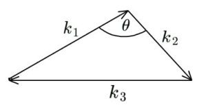
Throughout the paper we compare the FFT-bispectrum measurements to that of theory, but also to the bispectrum from a direct-measurement method.

3.1 Direct measurement of the bispectrum

To evaluate the performance of the FFT bispectrum estimator, it is desirable to draw comparison with another algorithm. We therefore use a restricted implementation of the direct-measurement method, which has been designed to reduce calculation time, and make the measurements presented here computationally tractable.

The main reason one would like to have a faster estimator for the bispectrum, or any other higher order polyspectra, is because the conventional direct estimators (that directly implement Equation LABEL:eq:bi_definition in their algorithm) of such polyspectra, require a significant amount of computational time. To implement Equation LABEL:eq:bi_definition in the direct algorithm of bispectrum, one would typically need to go through six nested for loops, each the size of the FFT box side in grid units. Such a nested loop is very computationally expensive.

To reduce the number of nested loops, we introduce two constraints on $\mbox{\boldmath${k}$}_{1}$ and $\mbox{\boldmath${k}$}_{2}$ in our direct-estimation algorithm. For a specific kind of triangle configuration, the ratio between the two arms of the triangle must remain constant, i.e.

$$k_{2}/k_{1}=m\,,$$ (16)

and the cosine of the angle ($\alpha=\pi-\theta$) between the two vector arms of the triangle must be fixed to,

$$\frac{\mbox{\boldmath${k}$}_{1}\cdot\mbox{\boldmath${k}$}_{2}}{k_{1}k_{2}}=\cos\alpha\,.$$ (17)

Implementation of these two constraints in the algorithm requires four nested for loops rather than six. This reduces the total number of steps in the algorithm to $N^{4}$, instead of $N^{6}$. where $N$ is the number of steps corresponding to each for loop.

In this algorithm, the first three for loops determine all possible values of the three components of the $\mbox{\boldmath${k}$}_{1}$ vector, and the fourth for loop determines all possible values of the one component of the $\mbox{\boldmath${k}$}_{2}$ vector. The other two components of the $\mbox{\boldmath${k}$}_{2}$ vector are fixed by Equations 16 and 17 for a given $\mbox{\boldmath${k}$}_{1}$ vector, and a single component of the $\mbox{\boldmath${k}$}_{2}$ vector. The $\mbox{\boldmath${k}$}_{3}$ vector is determined using the closure condition of the triangle. Once all components of $\mbox{\boldmath${k}$}_{1}$, $\mbox{\boldmath${k}$}_{2}$ and $\mbox{\boldmath${k}$}_{3}$ vectors are determined, one can take the product of the $\Delta(\mbox{\boldmath${k}$})$s corresponding to these three vectors, which will be a complex number (as are all $\Delta({\bf k})$s). If the actual field for which one intends to estimate the bispectrum is real it can easily be shown (using complex algebra and the Hermitian condition mentioned before) that the bispectrum will also be real. Thus, we take only the real part of this complex product as our bispectrum contribution to each bin. We also estimate the power spectrum contribution from each of the three arms of the triangle in three separate bins, corresponding to $P(k_{1})$, $P(k_{2})$ and $P(k_{3})$. In these power spectrum bins only $k$ vectors which satisfy the closure condition of Equation LABEL:eq:bi_definition contribute, and we use these $P(k)$s to estimate the Perturbation theory expectation for the bispectrum of N-body density fields as described by Equation LABEL:eq:PT_Bi in Section 3.2.

This particular algorithm for direct estimation of bispectrum is very restrictive in nature when compared to the fast algorithm upon which this paper is focused. While the fast algorithm allows any kind of bin width around the target $\mbox{\boldmath${k}$}_{1}$, $\mbox{\boldmath${k}$}_{2}$ and $\mbox{\boldmath${k}$}_{3}$ vectors, corresponding to a specific triangle configuration, in this direct algorithm one can only put a bin width around $\mbox{\boldmath${k}$}_{1}$ but it is not possible to put any bin widths around $\mbox{\boldmath${k}$}_{2}$ and $\mbox{\boldmath${k}$}_{3}$, as their components are determined precisely by Equations 16, 17 and the closure condition of a triangle for a specific set of components of $\mbox{\boldmath${k}$}_{1}$. Due to this difference in the nature of binning in these two algorithms, they will be probing bispectrum for a slightly different sets of triangles, when averaged across their respective $k$ bins. We thus do not expect a direct one-to-one exact match/correspondence between these two methods while comparing the bispectrum estimated by them.

3.2 Non-linear density field - A slightly non-Gaussian test case

In testing our FFT estimator, it is useful to have theoretical predictions of the bispectrum with which to draw comparison. As such, it is useful to consider the bispectrum of the density field.

Perturbation theory describes the initial density field with a background term, and perturbative terms. Whilst the background term will have a vanishing three-point correlation function and bispectrum, the perturbative terms which evolve in a non-linear manner under gravity will exhibit non Gaussianities. Fry (1984) use perturbation theory, to second order (or tree level), to make a prediction for the ${k}$ dependence on the bispectrum of the matter density field, finding that,

$$\begin{split}B(k_{1},k_{2},k_{3})&=2F(k_{1},k_{2})P(k_{1})P(k_{2})+(\mathrm{cyc.})\\ F(k_{1},k_{2})&=\left(\frac{1+\kappa}{2}\right)+\left(\frac{\mbox{\boldmath${k}$}_{1}\cdot\mbox{\boldmath${k}$}_{2}}{2k_{1}k_{2}}\right)\left(\frac{k_{1}}{k_{2}}+\frac{k_{2}}{k_{1}}\right)\\ &+\left(\frac{1-\kappa}{2}\right)\left(\frac{\mbox{\boldmath${k}$}_{1}\cdot\mbox{\boldmath${k}$}_{2}}{k_{1}k_{2}}\right)^{2}\,,\\ \end{split}$$ (18)

where $\kappa=3/7\,\Omega_{\mathrm{m}}^{-1/143}$ as appropriate for a $\Lambda$CDM cosmology (Scoccimarro, 2000). This tree-level bispectrum prediction has been shown to under predict the bispectrum as measured from N-body simulations. This is especially true for scales corresponding to strongly non-linear scales, but theory still under predicts the N-body bispectrum on scales for which density fluctuations are small and still non-linear, e.g. (Scoccimarro et al., 1997). To compare our FFT-estimator measurements of the bispectrum with the predictions of tree-level perturbation theory, we use the Particle-Mesh N-body matter density simulations described by Mondal et al. (2014) and Bharadwaj & Srikant (2004). This simulation was run with a $4288^{3}$ grid, and a cube side of 300 Mpc. This provides a spatial resolution of $\sim 0.07$ Mpc, and mass resolution $1.09\times 10^{8}$ M_⊙. The boxes we analyse here have been coarse gridded to $536^{3}$.

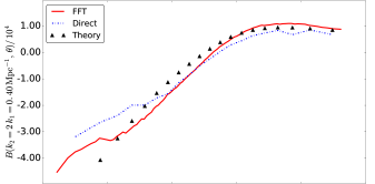
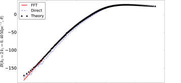
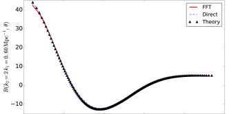
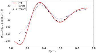
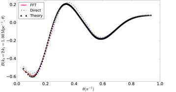
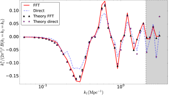
In Figures 2 to Figure 4 we plot the bispectrum, from a density simulation at $z=7$, as measured using the FFT bispectrum estimator of Equation LABEL:eq:Jeong_BI (red solid line), the direct-measurement method described at the beginning of this section (blue dot-dashed line) and as predicted by PT (black triangles), i.e. Equation LABEL:eq:PT_Bi. To highlight divergence between the direct and FFT methods due to differences their $k$ binning, we also plot the PT prediction binned as per our direct-measurement method (pink stars). We plot the bispectrum as a function of angle ($\theta$ in $\pi^{-1}$ radians) for $k_{2}=2\,k_{1}$ in Figure 2 and for $k_{2}=5\,k_{1}$ in Figure 3, with $k_{1}=(0.51,0.74,1.55)\,\mathrm{Mpc}^{-1}$ from top to bottom (note that in Figure 3 we do not plot $k_{1}=1.55\,\mathrm{Mpc}^{-1}$ as $k_{2}$ is greater than the Nyquist limit). Here we average over bins of $\cos(\theta)\pm 0.05$ for both direct and FFT estimators.

From these figures it is clear that the FFT estimator closely follows the PT theoretical predictions, only diverging on smaller scales (larger $k$-modes) as expected. The direct-measurement method also agrees well with the FFT estimator. We note that there is some divergence between the two methods for $k_{2}=3.10\,\mathrm{Mpc}^{-1}$ for $\theta\gtrsim 0.5\,\pi^{-1}$ radians, which is due to differences in the binning between the two methods. This is clear as we see the same qualitative divergence between the theoretical predictions resulting from each method’s binning.

$\begin{array}[]{c}\includegraphics[trim=42.67912pt 75.39963pt 14.22636pt 59.75095pt,clip={true},scale={0.25}]{Images/SumanMajumdar_densityB_vs_theta_DirectSM_cf_JeongCW_k1byk2_2.00k1_0.51JeongBinfac3.00_3.00_3.00_dk_0.01_536_300Mpc.pdf}\\ \includegraphics[trim=42.67912pt 75.39963pt 14.22636pt 59.75095pt,clip={true},scale={0.25}]{Images/SumanMajumdar_densityB_vs_theta_DirectSM_cf_JeongCW_k1byk2_2.00k1_0.74JeongBinfac3.00_3.00_3.00_dk_0.01_536_300Mpc.pdf}\\ \includegraphics[trim=42.67912pt 14.22636pt 14.22636pt 59.75095pt,clip={true},scale={0.25}]{Images/SumanMajumdar_densityB_vs_theta_DirectSM_cf_JeongCW_k1byk2_2.00k1_1.55JeongBinfac3.00_3.00_3.00_dk_0.01_536_300Mpc.pdf}\\ \end{array}$

Figure 2: Bispectrum measured from a non-linearly evolved density field. Pink stars mark the theoretical prediction as calculated using the same binning as the direct method. We plot the bispectrum as a function of angle between $k_{1}$ and $k_{2}$ where $k_{2}=2\,k_{1}$. From top to bottom we plot $k_{1}=(0.51,0.74,1.55)\,\mathrm{Mpc}^{-1}$ for which $k_{2}=(1.02,1.48,3.10)\,\mathrm{Mpc}^{-1}$ respectively. The grey shaded area corresponds to $k$ values beyond which Sefusatti et al. (2016) predict that the FFT bispectrum estimator will become inaccurate. Beyond divergence due to binning differences (clear by comparing the PT predictions under the two different binning schemes), the FFT estimator performs well, even in the grey shaded region.

$\begin{array}[]{c}\includegraphics[trim=49.79231pt 75.39963pt 14.22636pt 59.75095pt,clip={true},scale={0.25}]{Images/SumanMajumdar_densityB_vs_theta_DirectSM_cf_JeongCW_k1byk2_5.00k1_0.51JeongBinfac3.00_3.00_3.00_dk_0.01_536_300Mpc.pdf}\\ \includegraphics[trim=49.79231pt 14.22636pt 14.22636pt 59.75095pt,clip={true},scale={0.25}]{Images/SumanMajumdar_densityB_vs_theta_DirectSM_cf_JeongCW_k1byk2_5.00k1_0.74JeongBinfac3.00_3.00_3.00_dk_0.01_536_300Mpc.pdf}\\ \end{array}$

Figure 3: Bispectrum measured from a non-linearly evolved density field. Pink stars mark the theoretical prediction as calculated using the same binning as the direct method. We plot the bispectrum as a function of angle between $k_{1}$ and $k_{2}$ where $k_{2}=5\,k_{1}$. From top to bottom we plot $k_{1}=(0.51,0.74)\,\mathrm{Mpc}^{-1},k_{2}=(2.55,3.70)\,\mathrm{Mpc}^{-1}$ respectively, note that we cannot plot $k_{1}=1.55\,\mathrm{Mpc}^{-1}$ as this pushes $k_{2}$ beyond the Nyquist limit. The grey shaded area corresponds to $k$ values beyond which Sefusatti et al. (2016) predict that the FFT bispectrum estimator will become inaccurate. Again, the FFT estimator is seen to perform very well as compared to theory and our direct method.

$\begin{array}[]{c}\includegraphics[trim=35.56593pt 75.9688pt 14.22636pt 59.75095pt,clip={true},scale={0.25}]{Images/SM_BrealBnorm_vs_k_DirectSM_cf_JeongCW_equiJeongBinfac3.00_3.00_3.00_dk_2_536_300Mpc.pdf}\\ \includegraphics[trim=35.56593pt 8.5359pt 14.22636pt 59.75095pt,clip={true},scale={0.25}]{Images/SM_BrealB_vs_k_DirectSM_cf_JeongCW_equiJeongBinfac3.00_3.00_3.00_dk_2_536_300Mpc.pdf}\\ \end{array}$

Figure 4: Bispectrum measured from a non-linearly evolved density field. Pink stars mark the theoretical prediction as calculated using the same binning as the direct method. We plot the bispectrum as a function of $k_{1}$ for triangles where $k_{1}=k_{2}=k_{3}$. We show $B(k_{1}=k_{2}=k_{3})\,k_{1}^{6}/(2\pi^{2})^{2}$ in the top plot. In the bottom plot, we plot the average $|B(k)|$ across 5 different realisations as measured by the direct method (blue dot-dashed line). The beige shaded region marks the 1-$\sigma$ standard deviation across the 5 realisations. For this simulation, we find that $B(k)$ exhibits erratic evolution due fluctuations in sign caused by sample variance, the amplitude of the real part of the bispectrum is far more stable. The grey shaded area corresponds to $k$ values beyond which Sefusatti et al. (2016) predict that the FFT bispectrum estimator will become inaccurate. Other than differences from noise due to sample variance and differences in binning, the FFT estimator is seen to perform very well as compared to theory and our direct method.

The Nyquist theorem states that the smallest wavelength that may be resolved is 2 samples (in our case pixels), this corresponds to a limit on $k$ of,

$$\begin{split}k_{\mathrm{nyq}}=\frac{2\pi}{l_{\mathrm{nyq}}}=\frac{2\pi}{(2L/N_{\mathrm{side}})}=k_{\textsc{f}}N_{\mathrm{side}}/2\,.\end{split}$$ (19)

We therefore do not calculate the bispectrum for triangles that incorporate any $|\mbox{\boldmath${k}$}|\geq k_{\mathrm{nyq}}$. However, Jeong (2010) conclude the largest mode for which the FFT bispectrum estimator is stable (i.e. not affected by aliasing) is three times smaller than the 1D FFT grid, or $k=N_{\mathrm{side}}\,k_{\mathrm{f}}/3$. We mark this limit on all plots by a grey shaded region. This conclusion is reached by counting the triangles using the FFT approach (i.e. applying the denominator of Equation LABEL:eq:Jeong_BI), and comparing it to the true counted value.

An alternative theoretical argument for this limit, that relates to aliasing, is provided in Sefusatti et al. (2016). In equation LABEL:eq:delta_nr, we are essentially performing the following operation,

$$\begin{split}&B(\bm{k}_{1},\bm{k}_{2},\bm{k}_{3})=\\ &\frac{1}{N_{\mathrm{tri}}}\int d^{3}\mbox{\boldmath${x}$}\int_{k_{1}}d^{3}\mbox{\boldmath${q_{1}}$}\int_{k_{2}}d^{3}\mbox{\boldmath${q_{2}}$}\int_{k_{3}}d^{3}\mbox{\boldmath${q_{3}}$}\delta_{\bm{q}_{1}}\delta_{\bm{q}_{2}}\delta_{\bm{q}_{3}}\mathrm{e}^{i\,\bm{q}_{123}\cdot\bm{x}}\,,\\ \end{split}$$ (20)

where $\bm{q}_{123}=\bm{q}_{1}+\bm{q}_{2}+\bm{q}_{3}$, and the integrals are over grid points for which $\bm{q}_{i}=\bm{k}_{i}\pm\Delta k$ (where $\Delta k$ is the chosen bin width). Sefusatti et al. (2016) argue that the exponent in this expression is invariant under a 1-dimensional translation of each wavenumber of $(2\pi/L)\,(N_{\mathrm{side}}/3)$ for which $\bm{q}_{123}\rightarrow\bm{q}_{123}+2\pi N_{\mathrm{side}}/L$. The translation cancels with $\bm{x}=(L/N_{\mathrm{side}})\bm{m}$, introducing a factor of $\mathrm{exp}(i\,2\pi\bm{m})$. As $\bm{m}$ is an integer triplet the exponent associated with the transpose is always one. The argument is that this means that there is a periodicity in the phase term associated with this translation scale, which defines a maximum wavenumber, $k_{\mathrm{max}}=N_{\mathrm{side}}\,k_{\mathrm{f}}/3$, beyond which the estimator will become confused. If this argument stands, then $k_{\mathrm{max}}$ will decrease according to $k_{\mathrm{max}}(p)=N_{\mathrm{side}}\,k_{\mathrm{f}}/p$ for a $p^{\mathrm{th}}$-order polynomial.

In the results that follow, it appears that this confusion effect does not seem to seriously affect the performance of the estimator, at least for the datasets considered here. If we were to exactly implement a Dirac-delta function using a Fourier transform, as per Equation LABEL:eq:delta_sefusatti, $\bm{q}_{123}\equiv 0$, which makes sure that the triangle is closed, and so the exponential contribution is always 1. In using the FFT estimator on a discrete dataset, this is not the case, as $\bm{q}_{123}$ does not necessarily form a closed triangle, and so there is ‘noise’ introduced by the Kronecker-delta’s exponential contribution not being unity. Any confusion due to the periodicity of the exponential phase term described above (and originating from the FFT implementation of the Kronecker delta) must necessarily be within the level of the ‘noise’ inherent to the method as a whole. To minimise noise introduced by the FFT implementation of the Kronecker delta, we advocate using a bin width corresponding to one pixel when measuring the bispectrum with the FFT estimator and, if required, applying further binning subsequently.

When we consider the bispectrum normalised by $k^{6}/(2\pi^{2})^{2}$ for the equilateral configuration, as shown in the top plot of Figure 4, we see the bispectrum as measured by both direct and FFT methods, diverges from the theoretical at $k\gtrsim 1$ Mpc^-1 (note that, for the direct method, we average over bins of $\cos{\theta}=-0.5\pm 0.05$). This is not surprising as second-order perturbation theory cannot fully describe the non-linearities of an N-body density field. However, we also see that the FFT estimator and the direct-measurement method start to diverge from each other at $k$ slightly lower than $k_{\mathrm{max}}$ (which is marked by the dashed line). As the divergence does not start at exactly $k_{\mathrm{max}}$ and the theoretical predictions from the two methods also diverge in a qualitatively very similar way. We conclude that it is, at least in part, due to differences in binning between the two methods. We also find that the impact of confusion due to periodicity of the phase term of Equation LABEL:eq:delta_sefusatti seems to be negligible in the case when two of the vectors that make up the triangle are below $k_{\mathrm{max}}$. This is clear from the bottom plots of Figures 2 and 3 where we see the FFT-estimator and direct-measurement method remain in reasonable agreement even for angles corresponding to $k_{3}\geq k_{\mathrm{max}}$. There is slight divergence between the two methods, but it is more likely that this is due to differences in binning, as, again, the same qualitative divergence is seen when the theoretical predictions are binned as per each of the different methods.

At the other extreme of small-$k$ (large scales), there is also a limit below which the triangle count becomes too low, and the bispectrum gets impacted by sample variance. We find this to occur when $N_{\mathrm{tri}}<10^{7}$, as measured using the FFT approach. This corresponds to $k\lesssim(100/6)\,k_{\mathrm{f}}$, i.e. when the $k_{\mathrm{f}}$ corresponds to greater than 6% of the $k$ mode under consideration. Below this $k$ the estimators become increasingly noisy, and the sign of the bispectrum also fluctuates from positive to negative at random. This makes it very hard to interpret the signal, and where such wild fluctuations are seen, we argue it is better to plot the absolute value of the bispectrum. In Figure 4, we plot the average of $|B(k)|$ as measured by the direct method and its 1-$\sigma$ standard deviation (beige shaded region) across 5 different realisations of the density field. We find that that the impact of sample variance on $|B(k)|$ is less dramatic than it is for $B(k)$; for illustration, $\sim$50% of $B[k<(100/6)\,k_{\mathrm{f}}]$ (from direct-measurement) of a single realisation have negative sign. Apparent from Figure 4 is a divergence between the two methods at small $k$, but again this may be attributed to differences in binning between the two methods.

3.3 Toy-model for reionization - A highly non-Gaussian test case

Bharadwaj & Pandey (2005) present an analytical model for the bispectrum of the ionization field during reionization. To do so they assume that the ionized bubbles are randomly distributed spheres, all of a single radius $R$ (where $R$ is a free parameter). This radius is then used to define the number density of bubbles $\overline{n}_{\mathrm{H}\textsc{i}}$ through $1-\overline{x}_{\mathrm{H}\textsc{i}}=(4\pi R^{3}/3)\overline{n}_{\mathrm{H}\textsc{i}}$, with the neutral fraction $\overline{x}_{\mathrm{H}\textsc{i}}$ calculated according to the model of Zaldarriaga et al. (2004). In this model the power spectrum of the ionization field is given by,

$$\begin{split}P_{\mathrm{H}\textsc{i}}(k)=\frac{(1-\overline{x}_{\mathrm{H}\textsc{i}})^{2}W^{2}(kR)}{\overline{n}_{\mathrm{H}\textsc{i}}}\,,\end{split}$$ (21)

and the bispectrum by,

$$\begin{split}B_{\mathrm{H}\textsc{i}}(k_{1},k_{2},k_{3})=-\frac{(1-\overline{x}_{\mathrm{H}\textsc{i}})^{3}W(k_{1}R)W(k_{2}R)W(k_{3}R)}{\overline{n}_{\mathrm{H}\textsc{i}}^{2}}\,,\end{split}$$ (22)

where the window function $W(kR)$ is the Fourier transform of the spherical top hat function. We generate cubes that simulate the model of Bharadwaj & Pandey (2005), so that we may compare our estimator with the above theoretical predictions. Slices through two simulation cubes are shown in Figure 5. The left slice is at $z=14$ where reionization is just beginning when $x_{\mathrm{H}\textsc{i}}=0.99$; the right figure is at $z=11$ when $x_{\mathrm{H}\textsc{i}}=0.88$. As we see from the right slice of Figure 5, the bubbles are in some cases overlapping with each other. Such overlap is not allowed for in the model of Bharadwaj & Pandey (2005), therefore we do not expect that the bispectrum measured from these boxes will exactly agree with the theoretical predictions of Equations 21 and 22.

$\begin{array}[]{c}\framebox{\includegraphics[trim=0.0pt 0.0pt 0.0pt 0.0pt,clip={true},scale={0.19}]{Images/random_spheres_slice_z14_olap_allowed.png}}\framebox{\includegraphics[trim=0.0pt 0.0pt 0.0pt 0.0pt,clip={true},scale={0.19}]{Images/random_spheres_slice_z11_olap_allowed.png}}\\ \end{array}$

Figure 5: Slices through the randomly-placed ionized spheres model for reionization; white depicts 100% neutral regions and black 100% ionized regions. The left column shows the models at $z=11$, $x_{\mathrm{H}\textsc{i}}=0.99$ and the right column at $z=14$, $x_{\mathrm{H}\textsc{i}}=0.88$. For both the radius of all ionized spheres is 10 Mpc.

We analyse ionization boxes with 600 pixels and 600 Mpc on a side, because this is the resolution of the simulations of Watkinson & Pritchard (2015) from which we ultimately wish to study the bispectrum during the cosmic dawn and the EoR in future work. We arbitrarily set the radius of the bubbles to be 10 Mpc, choosing smaller bubbles to minimize the effect of overlap. Unlike the density simulations, the power spectrum from the model of Bharadwaj & Pandey (2005) is not monotonic in $k$. We therefore use this to test the FFT estimator for the power spectrum, i.e. Equation LABEL:eq:Jeong_PS. For direct estimation of the power spectrum we loop through the FT box and calculate $\langle\delta(k)^{2}\rangle$ for all $k$ that fall in a given bin. In Figure 6, we plot the spherically-averaged power spectrum normalised by $k^{3}/2\pi^{2}$, i.e. the dimensionless power spectrum. We find that there is good agreement between the FFT and direct methods, as well as with the theoretical prediction of Equation 21.

$\begin{array}[]{c}\includegraphics[trim=35.56593pt 14.22636pt 14.22636pt 59.75095pt,clip={true},scale={0.25}]{Images/random_ionised_spheres_overlapP_vs_k_DirectSM_cf_JeongCW_equi_z14.0_Binfac3.00_3.00_3.00_600_600Mpc.pdf}\\ \end{array}$

Figure 6: Spherically-averaged power spectrum from a simulation of reionization that assumes the ionization field consisting of randomly-distributed uniform-sized spherical bubbles. The FFT estimator, direct method and theory are perfectly in agreement for the spherically-averaged power spectrum with only slight divergence at very small scales, caused by overlap of ionized spheres being allowed in the simulations, but not in theory. The box analysed here have $z=14$ and $x_{\mathrm{H}\textsc{i}}=0.99$ (chosen to minimize differences between simulation and theory due to overlap).

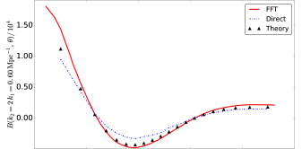
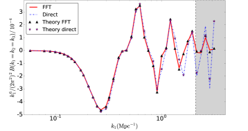
In Figure 7, we plot the bispectrum from the reionization simulation as a function of $\theta$ with $k_{2}=2\,k_{1}$ for $k_{1}=(0.2,0.3,0.5)\,\mathrm{Mpc}^{-1}$ and $k_{2}=(0.4,0.6,1.0)\,\mathrm{Mpc}^{-1}$ from top to middle-bottom respectively. The equilateral configuration is shown in the bottom row of Figure 7, here we normalise the bispectrum by $k^{6}/(2\pi^{2})^{2}$ to highlight the oscillatory nature of the signal. We bin the direct estimates of the bispectrum with $\cos(\theta)\pm 0.02$. The left column corresponds to $z=11$ when the neutral fraction is 0.88, and the right column to $z=14$ when the neutral fraction is 0.99.

There are a few interesting features of the bispectrum for this model, which are most clear in plots of the bispectrum for the equilateral configuration (see bottom row of Figure 7). As is to be expected there is a main peak around the $k$ associated with the bubble size, i.e. $k=2\pi/R$. Following this peak is a ringing due to the spheres having hard edges. There is also a negative minimum, in the normalised bispectrum, around the scale associated with twice the bubble size, this occurs because the unnormalised bispectrum plateaus towards a constant negative value with decreasing k, and then the signal is suppressed towards zero by the normalisation. Such features are defined by the window function and vary only in amplitude as the ionised fraction increases do to the presence of more spherical ionised bubbles.

We see that the bispectrum as measured by the FFT-bispectrum estimator follows the theoretical predictions very closely. Again the bispectrum becomes noisy due to sample variance for $k\lesssim(100/6)\,k_{\mathrm{f}}$, which for this dataset corresponds to $k\leq 0.17$ Mpc^-1. This is only evident in the unnormalised bispectrum, which we do not show here, and is far less pronounced for our ionization field than it is with the density field. For example, we do not see the sign of the bispectrum switching from negative to positive in this regime, as we do for the density field. It is likely that this is because our reionisation simulations are very simple; the ionization field is binary and so they will contain very little numerical noise as compared to the density field.

We again find that the estimator follows the theoretical predictions very closely where $k\geq k_{\mathrm{max}}$, this is most plain to see from the plots of equilateral configurations in the bottom row of Figure 7. For the $z=11$ model, we do see a slight divergence from theory at certain values of $k$. This is clearly due to the allowance of bubble overlap in the simulation, as can be seen by comparing the left and right columns of the bottom row of Figure 7. For example, we see that the FFT bispectrum estimator starts to diverge slightly from theory at $k<0.2$ at $z=11$, where $x_{\mathrm{H}\textsc{i}}\sim 0.9$, whereas it follows the theoretical predictions very closely when $z=14$, where $x_{\mathrm{H}\textsc{i}}\sim 0.99$.

Figure 7: Bispectrum from a simulation of reionization that assumes the ionization field is made up of randomly-distributed uniform-sized spherical bubbles. Pink stars mark the theoretical prediction as calculated using the same binning as the direct method. We plot configurations where $k_{2}=2\,k_{1}$ and $k_{1}=0.2\,\mathrm{Mpc}^{-1}$, $k_{2}=0.4\,\mathrm{Mpc}^{-1}$ (top), $k_{1}=0.3\,\mathrm{Mpc}^{-1}$, $k_{2}=0.6\,\mathrm{Mpc}^{-1}$ (middle-top), $k_{1}=0.5\,\mathrm{Mpc}^{-1}$, $k_{2}=1.0\,\mathrm{Mpc}^{-1}$ (middle-bottom), and the equilateral configuration (bottom). The evolution of the ionization field corresponds to $z=11$ and $x_{\mathrm{H}\textsc{i}}=0.88$ (left column) ,and $z=14$ and $x_{\mathrm{H}\textsc{i}}=0.99$ (right column). The grey shaded area corresponds to $k$ values beyond which Sefusatti et al. (2016) predict that the FFT bispectrum estimator will become inaccurate. As with the density field, the FFT estimator performs well, as differences between the two methods can be attributed to binning. This is underlined by how well each method follows the theory when calculated with the same binning scheme in the right column (at this stage overlap will be minimal and so differences between measurements from the simulation and theory due to overlap will be minimized).

3.4 Effect of binning in the direct estimator of bispectrum

As discussed in Section 3.1, there is a clear difference between the binning approaches of the two bispectrum algorithms discussed in this paper. When the bispectrum is an oscillatory function of $k$, increases to the $k$ bin width will cause the measured bispectrum to diverge dramatically from its true value. The bispectrum of the toy model, introduced in Section 3.3, is a perfect example of such a scenario. The behaviour of the bispectrum in this model is determined by the window function $W(kR)$, as shown in Equation 22, which is very oscillatory in nature. To reduce sample variance at small $k$ values for equilateral triangle configuration (i.e. $k_{1}=k_{2}=k_{3}$), if one increases the $k_{1}$ bin width significantly, one would essentially vary the $W(k_{1}R)$ function in the bin. If some of the $k_{1}$ values within the bin lie somewhere close to the dips of oscillations in $W(k_{1}R)$, the bispectrum estimation by different triangles contributing within bin will vary severely, as the change in amplitude near the dips of oscillation is large. Thus, the bin-averaged bispectrum in such a scenario will differ significantly from the theoretical expectation value of the bispectrum, as predicted by Equation 22, and as estimated using the mid-point or the average value of the $k$ mode in the respective bin. To avoid this we keep the $k$ bin width at its bare minimum. and thus the direct method’s bispectrum estimation for small $k$ values is more affected by sample variance for this toy model (see Figure 7).

For other triangle configurations, where $k_{1}\neq k_{2}\neq k_{3}$, the situation would be a bit more complicated, as each of the window function contributing to the bispectrum for that triangle will probe different parts of this oscillatory window function and their product will give rise to “beats”. Different triangles within the same bispectrum estimation bin will thus produce different beats for the oscillatory window function, and their average value across the bin will be very different than the theoretical prediction for the mid point of the bin. To demonstrate this point more clearly, we estimate the theoretical bispectrum, following Equation 22, for each of the triangles contributing within a bin, and plot the bin-averaged theoretical value, this is shown by the pink stars in Figure 7. We observe that the bin averaged theoretical prediction follows the numerical estimation very closely.

This discussion makes it clear that great care must be taken when using our direct method to measure highly oscillatory bispectrum signals, such as that of the toy model for the ionization field explored here. However, this toy model is very limited in nature as it assumes all ionized regions in the IGM to be spheres of equal radius $R$, at every stage of the EoR. In reality, the ionized regions, at any stage of reionization, will be of different shapes and volumes. This has been observed by various reionization simulations to date (e.g. Majumdar et al. 2014; Iliev et al. 2015). If we consider that at any redshift during reionzation the size of the ionized spheres are uniformly distributed between $R_{\mathrm{min}}\leq R\leq R_{\mathrm{max}}$, and so the resulting 21-cm signal will be proportional to $\sum_{i}W(kR_{i})$. It can be shown that even for a moderate range of values of $R_{i}$, unlike $W(kR)$, $\sum_{i}W(kR_{i})$ is a smooth function of $k$. Thus, it will be safe to use the direct estimator of bispectrum in such a scenario. We discuss this in more details in our follow up work Majumdar et al. (in prep).

4 Conclusion

In this paper we have presented the derivation of a fast estimator for the polyspectra. We outline an algorithm that provides a further speed up by initialising an indexing array in which each $j$ index contains an array of all FFT-box co-ordinates that correspond to $k$-vectors of a particular length (connected to the array element index $j$ by a scaling factor). This removes the need to fully loop through the FFT-box for every bispectrum call.

As we intend to apply this approach to study the bispectrum of the 21-cm signal, we focus our tests of this algorithm on the bispectrum. We test this FFT-bispectrum algorithm for the bispectrum using a non-linear N-body density field (a mildly non-Gaussian dataset), and a toy model for reionization consisting of mono-sized ionized spheres. For both cases our FFT-bispectrum algorithm reproduces the bispectrum predicted by theory and measured using a direct-measurement algorithm. We find that the algorithm behaves reasonably well in both test cases at $k>k_{\mathrm{max}}$, where it has previously been argued that the estimator should break down. The argument is that a periodicity in the phase term of the Kronecker-delta function (when enforced using FFTs) will cause the estimator to become inaccurate beyond $k_{\mathrm{max}}$. We argue that the reason we do not see the estimator break down, is because the impact of this periodicity will be within the magnitude of inaccuracy introduced by using FFTs to enforce the Kronecker delta, which is inherent to the estimator at all $k$. This inaccuracy occurs as the contribution from the Kronecker-delta term is not exactly unity, this is because discretised $k$ vectors often do not form perfectly closed triangles. We therefore suggest that the FFT-bispectrum estimator may still be applied in this regime. We also advocate using a bin width of just one pixel when measuring the bispectrum with the FFT estimator, and applying any desired binning subsequently.

At low $k$, both estimators become noisy due to sample variance, and this can cause erratic behaviour, including the sign of the bispectrum randomly flipping from negative to positive, and vice versa. This erratic behaviour can be suppressed by plotting the amplitude of the bispectrum, with the drawback of suppressing genuine sign changes in the signal, which may contain important information.

The FFT-polyspectra algorithm presented in this paper is faster than direct-measurement methods and is fast enough to be used in sampling problems. Given the non-Gaussianity of the 21-cm signal during the cosmic dawn and reionization, this estimator will be invaluable for performing parameter estimation. Furthermore, whilst we focus on cosmological datasets, this algorithm will be very valuable for any non-Gaussian dataset.

References

- (1) Ali et al., 2015, ApJ, 809, 61
- Beardsley et al. (2016) Beardsley et al., 2016, ApJ, 833, 19
- Bharadwaj & Pandey (2005) Bharadwaj S., Pandey S. K., 2005, MNRAS, 358, 968
- Bharadwaj & Srikant (2004) Bharadwaj S., Srikant P. S., 2004, J. Astrophys. & Astron., 25, 67
- Bowman & Rogers (2010) Bowman J. D., Rogers A. E. E., 2010, Nature, 468, 796
- Burns et al. (2012) Burns J. O. et al., 2012, Adv. Sp. Res., 49, 433
- Byun et al. (2017) Byun, J. et al., 2017, MNRAS, 471, 2, 1581
- DeBoer et al. (2017) DeBoer, D. R. et al., 2017, PASP, 129, 045001
- Dixon et al. (2015) Dixon K. L. et al., 2015, MNRAS, 456, 3011
- Feldman et al. (2001) Feldman H. A. et al., 2001, Phys. Rev. Lett., 86, 8, 1434
- Field (1958) Field G. B., 1958, Proc. IRE, 46, 240
- Field (1959) Field G. B., 1959, ApJ, 129, 536
- Friedrich et al. (2010) Friedrich, M. M. et al., 2010, MNRAS, 413, 2, Pp. 1353
- Kakiichi et al. (2017) Kakiichi, K. et al., 2017, arXiv:1702.02520
- Fry (1984) Fry J. N., 1984, ApJ, 279, 499
- Gil-Marín et al. (2016) Gil-Marín H. et al., 2016, MNRAS, 465, 1757
- Harker et al. (2009) Harker G. J. A. et al., 2009, MNRAS, 393, 1449
- Iliev et al. (2015) Iliev I. T. et al., 2015, Advancing Astrophysics with the Square Kilometre Array (AASKA14), arXiv:1501.04213
- Jeong (2010) Jeong D., 2010, Cosmology with high ( z > 1 ) redshift galaxy surveys., PhD thesis, The University of Texas at Austin
- Komatsu et al. (2002) Komatsu E. et al., 2002, ApJ, 566, 1, 19
- Loeb & Furlanetto (2013) Loeb A., Furlanetto S. R., 2013, The First Galaxies in the Universe. Princeton University Press
- Majumdar et al. (2014) Majumdar S. et al., Bharadwaj S., Friedrich M. M., 2014, MNRAS, 443, 2843
- (23) Mellema et al., 2013, Exp. Astron., 36, 235
- Mondal et al. (2014) Mondal R. et al., 2014, MNRAS Lett., 449, L41
- Mondal et al. (2016) Mondal R., Bharadwaj S., & Majumdar S., 2016, MNRAS, 64, 3, 2992
- Patil et al. (2017) Patil, A. H. et al., 2017, ApJ, 838, 65
- Planck Collaboration (2015) Planck Collaboration, Planck 2015 results. XVII, 2015, 594, 66, 594.
- Pritchard & Loeb (2012) Pritchard, J. R., & Loeb, A., 2012, Rep. Prog. Phys., 75, 8
- Regan et al. (2011) Regan, D. et al., 2011, Phys. Rev. D, 86, 12
- Schmittfull et al. (2012) Schmittfull, M. M., Regan, D. M., & Shellard, E. P. S., 2012, Phys. Rev. D, 88, 6
- Schneider et al. (2015) Schneider A. et al., 2016, J. Cosmol. Astropart. Phys., 4, 47
- Scoccimarro (2015) Scoccimarro R., 2015, Phys. Rev. D, 92, 8
- Scoccimarro (2000) Scoccimarro R., 2000, ApJ, 544, 597
- Scoccimarro et al. (2001) Scoccimarro R. et al., 2001, ApJ, Vol., 546, 2, 652
- Scoccimarro et al. (1997) Scoccimarro, R. et al., 1997, ApJ, 496, 586.
- Sefusatti (2005) Sefusatti E., 2005, Probing fundamental physics with large-scale structure: From galaxy formation to inflation., PhD thesis, New York University
- Sefusatti et al. (2016) Sefusatti E. et al., 2016, MNRAS, 460, 4, 3624
- Shimabukuro et al. (2016) Shimabukuro H. et al., 2016, MNRAS, 458, 3, 3003
- Shimabukuro et al. (2016a) Shimabukuro, H. et al., 2016a, MNRAS, 468, 2, 1542
- Shimabukuro et al. (2015) Shimabukuro H. et al., 2015, MNRAS, 451, 467
- Singh et al. (2017) Singh, S. et al., 2017, preprint, arXiv:1703.06647
- Slepian & Eisenstein (2015) Slepian, Z., & Eisenstein, D. J., 2015, MNRAS Lett., 455, 1, L31
- Watkinson & Pritchard (2014) Watkinson C. A., Pritchard J. R., 2014, MNRAS, 443, 3090
- Watkinson & Pritchard (2015) Watkinson C. A., Pritchard J. R., 2015, MNRAS, 454, 1416
- Watkinson et al. (2015) Watkinson C. A. et al., 2015, MNRAS, 449, 3202
- Zaldarriaga et al. (2004) Zaldarriaga M., Furlanetto S. R., Hernquist L., 2004, ApJ, 608, 622