Cooling Stochastic Quantization with colored noise

Abstract

Smoothing of field configurations is highly important for precision calculations of physical quantities on the lattice. We present a cooling method based on Stochastic Quantization with a built-in UV momentum cutoff. The latter is implemented via a UV-regularized, hence colored, noise term.

Our method is tested in a two-dimensional scalar field theory. We show, that UV modes can be removed systematically without altering the physics content of the theory. The approach has an interpretation in terms of the non-perturbative (Wilsonian) renormalization group that facilitates the physics interpretation of the cutoff procedure. It also can be used to define the maximal colored cooling applicable without changing the theory.

I Introduction

Lattice field theory is a powerful non-perturbative approach that allows for ab initio calculations of realistic quantum field theories. It has been applied to many areas of physics ranging from condensed matter systems to quantum gravity. In nuclear physics applications range from the details of the hadronic spectrum to the numerical study of topological properties and configurations in Yang-Mills theory and Quantum Chromodynamics (QCD). A further task for lattice field theory and other non-perturbative approaches is to map out the phase structure of strongly correlated systems. However, lattice simulations for finite density QCD are hampered by the sign problem. This situation has triggered a plethora of work in this direction, for a recent review see Aarts (2016).

Amongst the contenders for beating the sign problem Stochastic Quantization based on a complex Langevin equation (CLE) is a very promising candidate Aarts et al. (2016a). The complexification however is non-trivial, see e.g. Aarts et al. (2013a) for a brief account and Aarts et al. (2017) for a state of the art. If applied to gauge theories it has to be equipped with cooling algorithms such as gauge cooling Seiler et al. (2013) in order to even achieve convergence. The CLE has been applied to explore the phase diagram of QCD and that of related models Sinclair and Kogut (2016); Nagata et al. (2016); Langelage et al. (2014); Aarts et al. (2016b).

Cooling algorithms, see e.g. Teper (1985), are set-up to eliminate configurations that carry large ultraviolet fluctuations. They are based on the assumption that physics scales can be safely separated from the ultraviolet scales where cooling is applied. Then, cooling simply improves the signal-to-noise ratio without altering the physics under investigation. For example, this works very well for observables such as the action density or the topological charge density. However, if cooling is not stopped it produces classical configurations for large cooling times. Hence, the crucial question is that after a well-defined stopping time. This stopping time can be related to the physical scale of the cooled theory of interest, see e.g. Garcia Perez et al. (1999). The same intricacy also is present for the recently put forward gradient flow cooling Lüscher (2010); Narayanan and Neuberger (2006); Gonzalez-Arroyo and Okawa (2013); Datta et al. (2016); Capponi et al. (2016), for further applications see Kagimura et al. (2015); Bornyakov et al. (2015). A comparison of the two approaches can be found in Bonati and D’Elia (2014).

In the present work we suggest to use the Stochastic Quantization approach cooled with colored noise. This combines a Langevin equation (LE) with the gradient flow. To that end we first notice that the Langevin equation without noise simply is the gradient flow. Hence, removing the noise for high momentum modes above a UV cutoff scale $\Lambda$ leaves us with a gradient flow for these modes. Then, the related colored noise Langevin evolution completely removes the momentum modes with $p^{2}>\Lambda^{2}$. In summary, a Langevin equation with such a colored noise introduces a UV momentum cutoff $\Lambda$ to the path integral. By varying the cutoff $\Lambda$ we interpolate between the full quantum evolution characterized by the LE with Gaussian white noise ($\Lambda\to\infty$) and the classical evolution characterized by the gradient flow ($\Lambda=0)$. This approach is closely related to the concept of stochastic regularization Bern et al. (1985, 1987).

Here, our approach is put to work in a scalar theory and numerical results are presented in two dimensions. Colored noise is also related to standard Kadanoff block spin steps Kadanoff (1966), as well as to the realization of the latter within the functional renormalization group, for reviews see e.g. Berges et al. (2002); Polonyi (2003); Pawlowski (2007); Delamotte (2012); Rosten (2012); Metzner et al. (2012). We show that a large regime of ultraviolet fluctuations can be removed without altering the physics content of the theory. Hence, cooling with colored noise can significantly reduce the numerical costs of lattice simulations done within Stochastic Quantization. Such a procedure could in principle also be applied to CLE simulations.

The paper is organized as follows. In section II we recall basic concepts of Stochastic Quantization and introduce stochastic regularization. The lattice field theory formulation of the LE with colored noise is described in section III. In section IV we review real scalar field theory on the lattice providing a suitable model for our numerical studies. This is followed by the discussion of the relation between colored noise and the renormalization group in section V. In section VI we discuss numerical results from simulations with colored noise. The approach is put to work in section VII, where also its relation to the functional renormalization group is discussed and utilized. We finish with our conclusions in section VIII.

II Stochastic quantization with colored noise

In this section we briefly review the main concepts of Stochastic Quantization and stochastic regularization within the example of a Euclidean real scalar field theory with the action $S=S[\phi]$.

Stochastic Quantization is based on the fact that a Euclidean quantum field theory can be described by a classical statistical mechanical system in thermal equilibrium with a heat reservoir Parisi and Wu (1981); Damgaard and Huffel (1987). This is formulated in terms of a stochastic process with a stationary distribution $\exp(-S[\phi])/Z$, where

$$Z=\int\mathcal{D}\phi\,\exp(-S[\phi])$$ (1)

denotes the partition function. The stochastic process evolves the fields according to the corresponding Langevin equation in a Langevin-time $\tau$

$$\frac{\partial\phi(x,\tau)}{\partial\tau}=-\frac{\delta S}{\delta\phi(x,\tau)}+\eta(x,\tau)\,.$$ (2)

Here, $\phi(x,\tau)$ denotes the $\tau$-dependent scalar field and $\eta(x,\tau)$ is the white noise field representing the quantum fluctuations. With vanishing noise the solution of the Langevin evolution converges to a solution of the classical equations of motion. The white noise is characterized by Gaussian distributed random numbers with

$$\langle\eta(x,\tau)\rangle =0\,,$$

$$\langle\eta(x,\tau)\,\eta(y,\tau^{\prime})\rangle =2\,\delta^{(d)}(x-y)\,\delta(\tau-\tau^{\prime})\,.$$ (3)

In the limit $\tau\to\infty$ thermal equilibrium is reached and the equal Langevin-time correlation functions of the statistical mechanical system converge to the Green’s functions of the Euclidean quantum field theory. The real Langevin evolution (2) can be applied as an updating algorithm in lattice simulations to sample field configurations from the Boltzmann distribution.

For a given Langevin equation there is an associated Fokker-Planck equation. The latter describes the Langevin-time evolution of a probability distribution function $P(\phi,\tau)$ and reads

$$\frac{\partial P(\phi,\tau)}{\partial\tau}=$$

$$\int\textrm{d}^{d}{x}\frac{\delta}{\delta\phi(x,\tau)}\left(\frac{\delta S}{\delta\phi(x,\tau)}+\frac{\delta}{\delta\phi(x,\tau)}\right)P(\phi,\tau)\,.$$ (4)

One can verify that the Boltzmann distribution $\exp(-S[\phi])$ is therefore the stationary distribution of (4) with $\partial_{\tau}P(\phi,\tau)=0$. More generally, if the action is real and positive semi-definite a stationary distribution of the Fokker-Planck equation exists which equals $\exp(-S[\phi])$ and the solution converges exponentially fast Damgaard and Huffel (1987); Aarts et al. (2013b). In summary, Stochastic Quantization provides an alternative to the standard quantization approach based on the path integral formalism.

In the Langevin formulation the noise containing the quantum fluctuations can be regularized in the ultraviolet by introducing a cutoff parameter $\Lambda$ Bern et al. (1987). The altered stochastic process in terms of the Langevin equation with a colored noise kernel then reads

$$\frac{\partial\phi(x,\tau)}{\partial\tau}=-\frac{\delta S}{\delta\phi(x,\tau)}+r_{\Lambda}(\Delta_{x})\,\eta(x,\tau)\,,$$ (5)

where the dimensionless regularization function $r_{\Lambda}(\Delta_{x})$ is a function of the ratio $\Delta_{x}/\Lambda^{2}$ of the Laplace operator and the square of the cutoff $\Lambda$. Using a short-hand notation for the functional derivatives, see app. D, the associated Fokker-Planck equation is

$$\frac{\partial P(\phi,\tau)}{\partial\tau}=\int\mathrm{d}^{d}x\frac{\delta}{\delta\phi_{x}}\left(\frac{\delta S}{\delta\phi_{x}}+\,r_{\Lambda}^{2}(\Delta_{x})\,\frac{\delta}{\delta\phi_{x}}\right)P(\phi,\tau)\,.$$ (6)

Note, that with $r_{\Lambda}(\Delta_{x})\to 1$ in the limit $\Lambda\to\infty$ the full quantum theory is recovered. For a detailed derivation of the Fokker-Planck equation from the Langevin equation with a noise kernel see Appendix D. Note, that the regularization function can be chosen in different ways. A simple and intuitive choice of the regularization function is a sharp cutoff in momentum space

$$r_{\Lambda}(p^{2})=\theta(\Lambda^{2}-p^{2})\,.$$ (7)

Using (7) in the Fokker-Planck equation (6) allows for a simple relation of Stochastic Quantization with colored noise with functional renormalization group equations, for reviews see Berges et al. (2002); Polonyi (2003); Pawlowski (2007); Delamotte (2012); Rosten (2012); Metzner et al. (2012). A solution of the fixed point equation $\partial_{\tau}P=0$ in momentum space is given by

$$P_{\Lambda}(\phi,\tau)=\exp\left(-S-\Delta S_{\Lambda}\right)\,,$$ (8)

with the cutoff term

$$\Delta S_{\Lambda}[\phi]=\frac{1}{2}\int_{p}\phi_{p}\,\Lambda^{2}\left(\frac{1}{r_{\Lambda}(p^{2})}-1\right)\phi_{-p}\,.$$ (9)

Inserting (8) with (9) into (6) we are led to the fixed point equation

$$\left[\Bigl{(}1-r_{\Lambda}(p^{2})\Bigr{)}\frac{\delta S}{\delta\phi_{p}}-r_{\Lambda}(p^{2})\frac{\delta\Delta S_{\Lambda}}{\delta\phi_{p}}\right]P_{\Lambda}(\phi,\tau)=0\,.$$ (10)

Both terms in the square brackets in (10) vanish for $p^{2}<\Lambda^{2}$ as they are proportional to $1-r_{\Lambda}(p^{2})$. Note that in the second term this comes from $r_{\Lambda}(1/r_{\Lambda}-1)=1-r_{\Lambda}$. In turn, for $p^{2}>\Lambda^{2}$ the measure $P(\phi,\tau)$ vanishes and hence (10) is satisfied for all fields and momenta. In summary, this entails that the ultraviolet modes satisfy the classical equations of motion and no quantum effects are taken into account. For more details on the connection between the kerneled Fokker-Planck equation and the functional renormalization group see Appendix E.

The regularization function (7) defines the colored noise field

$$\eta_{\text{col}}(p,\tau):=\eta(p,\tau)\,\theta(\Lambda^{2}-p^{2})\,,$$ (11)

with the space-time representation

$$\eta_{\text{col}}(x,\tau)=\frac{1}{(2\pi)^{d}}\int\,\mathrm{d}^{d}p\,\eta_{\text{col}}(p,\tau)\,\mathrm{e}^{-ip\cdot x}\,.$$ (12)

This leads us to the Langevin equation with colored noise

$$\frac{\partial\phi(x,\tau)}{\partial\tau}=-\frac{\delta S}{\delta\phi(x,\tau)}+\eta_{\text{col}}(x,\tau)\,,$$ (13)

which is used throughout the work. A visualization of the colored noise $\eta_{\text{col}}(x,\tau)$ in (12) with the sharp cutoff (11) is illustrated in Fig. 1.

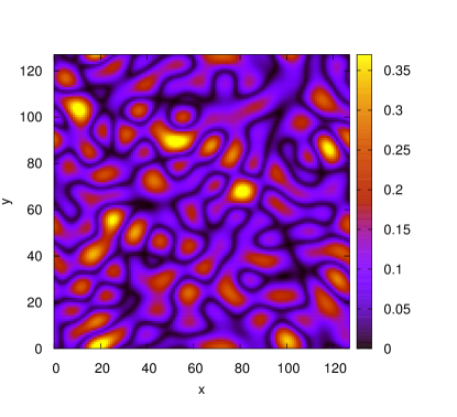
Figure 1: Heat map plot of the absolute value of colored noise on a 128 x 128 lattice for momentum cutoff ${s_{\Lambda}}=8$ (see Sec. III for the definition of the lattice cutoff). In contrast to the white noise picture described in (3) non-delta like spatially correlated structures extending over several lattice spacings are visible. The arrangement of the structures however appears to be random for we require the UV-modified stochastic process to remain Markovian.

III Lattice QFT with colored noise

In this section we present the implementation of our method for lattice simulations of Euclidean quantum field theories. We consider finite isotropic space-time lattices with lattice spacing $a$ and $N$ lattice points in each direction. Hence, the physical volume is $\Omega=(aN)^{d}$. Then, the allowed lattice momenta on the dual momentum lattice are given by

$$p_{\mu}=\frac{2\pi}{a\,N}\,n_{\mu}\,,\qquad{\rm with}\qquad\mu=1,\ldots,d\,,$$ (14)

where $n_{\mu}=-N/2+1,\ldots,N/2$. In the thermodynamic limit $N\to\infty$ the $d$-dimensional Brillouin zone is given by the interval $(-\pi/a,\pi/a]^{d}$.

In lattice simulations using the Langevin equation with colored noise we work with the sharp regulator (7) introduced in the previous section. Similarly as in the continuum, colored noise is generated by cutting off the noise modes on the momentum lattice followed by a discrete Fourier transformation back to the real space lattice which leads to

$$\eta_{\text{col}}(x,\tau)=\frac{1}{\Omega}\,\sum_{p}\,\mathrm{e}^{ip\cdot x}\,r_{\Lambda}(p^{2})\,\eta(p,\tau)\,.$$ (15)

The discretized Langevin equation with colored noise thus reads

$$\phi(x,\tau_{n+1})=\phi(x,\tau_{n})-\frac{\delta S}{\delta\phi(x,\tau_{n})}\,\Delta\tau+\sqrt{\Delta\tau}\,\eta_{\text{col}}(x,\tau_{n})$$ (16)

with the Langevin time step $\Delta\tau$. In our implementation we retain noise modes with $p^{2}\leq\Lambda^{2}$ and remove larger modes, see Fig. 2. Modes are being removed as the decreasing cutoff $\Lambda$ sweeps over the discrete lattice momenta. Note that the lattice theory only changes at the discrete values $\Lambda={s_{\Lambda}}\pi/a$ with

$${s_{\Lambda}}=\max\left(\frac{1}{\sqrt{d}}\sqrt{n_{\mu}^{2}}\right)\quad{\rm with}\quad p^{2}(n_{\mu})\leq\Lambda^{2}\,.$$ (17)

For the $\Lambda$-dependence see Fig. 3. For these values the cutoff $\Lambda$ sweeps over the discrete momentum values, see Fig. 2 for a two-dimensional dual lattice. We also notice that integer values of ${s_{\Lambda}}$ indicate a standard cubic momentum lattice of non-zero quantum fluctuations. Moreover ${s_{\Lambda}}=N/2$ corresponds to the standard Langevin evolution with Gaussian white noise. For ${s_{\Lambda}}=0$ only the zero-momentum mode contributes to the colored noise. For the simulation with the gradient flow we use the Langevin equation with the noise term set to zero.

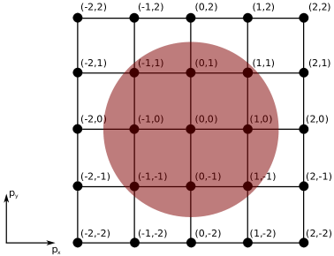
Figure 2: Schematic illustration of the dual lattice in $d=2$ describing our implementation of the cutoff. The radius of the red shaded circle corresponds to the cutoff $\Lambda$. Noise modes outside of the circle have zero weight in the Langevin evolution. Colored noise only receives finite contributions for momentum modes from inside the red circle.

For the further discussion it is useful to split the full field in momentum space in a classical and quantum contribution,

$$\phi(p)=\phi_{\text{\tiny{cl}}}(p)+\delta\phi_{\text{\tiny{qu}}}(p)\,,$$ (18)

with

$$\delta\phi_{\text{\tiny{qu}}}(p)=0\quad{\rm for}\quad p^{2}>{s_{\Lambda}}^{2}\,.$$ (19)

Note that the field $\delta\phi_{\text{\tiny{qu}}}$, that carries the quantum fluctuations, lives on the momentum lattice defined by $p^{2}\leq{s_{\Lambda}}^{2}$. Henceforth we call this generically smaller lattice the quantum lattice. In turn, the classical field $\phi_{\text{\tiny{cl}}}$ lives on the full momentum lattice which we therefore call the classical lattice. In position space this translates into a fine classical lattice and a coarser quantum lattice.

IV Scalar field theory

IV.1 Lattice formulation

Scalar field theories on the lattice have been investigated in numerous works over the recent decades and their applications range over a broad spectrum of topics involving particle, statistical and condensed matter physics. Here, we consider a Euclidean real single-component scalar field theory in $d$ dimensions with lattice action

$$S= \sum_{x}a^{d}\left[\frac{1}{2}\sum_{\mu=1}^{d}\frac{(\phi_{0}(x+a\hat{\mu})-\phi_{0}(x))^{2}}{a^{2}}\right.$$

$$\hskip 34.14322pt\left.+\frac{m_{0}^{2}}{2}\phi_{0}^{2}+\frac{g_{0}}{4!}\phi_{0}^{4}\right]\,,$$ (20)

where $\hat{\mu}$ denotes the unit vector in $\mu$-direction. The subscript $0$ indicates bare quantities, i.e. the bare mass $m_{0}$, the bare coupling $g_{0}$ and the bare field $\phi_{0}$ in the action. For numerical simulations the action is cast in the following dimensionless form

$$S=\sum_{x}\left[-2\kappa\sum_{\mu=1}^{d}\phi(x)\phi(x+\hat{\mu})\right.\\ \left.+\,\vphantom{\sum_{\mu=1}^{d}}(1-2\lambda)\,\phi(x)^{2}+\lambda\,\phi(x)^{4}\right]\,.$$ (21)

Figure 3: ${s_{\Lambda}}(\Lambda)$ for $N=4$ in two dimensions. The integer values of ${s_{\Lambda}}$ characterize the standard cubic momentum lattices. The latter will be used in the further analysis.

The parameter $\kappa$ is the so-called hopping parameter and $\lambda$ describes the quartic coupling of the theory. Note that here, the parameters $\kappa$ and $\lambda$ are positive. They are related to the bare mass, bare coupling and the lattice spacing in the following way

$$a^{\frac{d-2}{2}}\phi_{0} =(2\kappa)^{1/2}\,\phi\,,$$

$$(am_{0})^{2} =\frac{1-2\lambda}{\kappa}-2d\,,$$

$$a^{-d+4}\,g_{0} =\frac{6\lambda}{\kappa^{2}}\,,$$ (22)

where we have introduced the dimensionless field $\phi\,.$ The white noise Langevin update step ($\tau_{n}\to\tau_{n+1}$) of a field variable at lattice point $x$ is given by

$$\phi(x,\tau_{n+1})=\phi(x,\tau_{n})+K[\phi(x,\tau_{n})]\Delta\tau+\sqrt{\Delta\tau}\,\eta(x,\tau_{n})\,,$$ (23)

where the drift term $K[\phi(x)]=-\delta S[\phi]/\delta\phi(x)$ explicitly reads

$$K[\phi(x)] =2\kappa\sum_{\mu=1}^{d}[\phi(x+\hat{\mu})+\phi(x-\hat{\mu})]$$

$$\hskip 10.0pt+2\phi(x)\,(2\lambda\,(1-\phi(x)^{2})-1)\,.$$ (24)

The process (23) can be solved iteratively by using an explicit Euler-Maruyama discretization scheme. Higher order Runge-Kutta schemes are possible as well and are discussed in Damgaard and Huffel (1987); Batrouni et al. (1985).

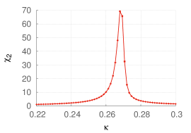
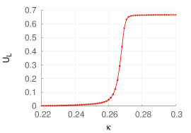
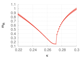
Figure 4: The phase diagram of $O(1)$ scalar field theory on the lattice characterized by three of the main observables, here at (fixed) coupling $\lambda=0.02$ for a $32\times 32$ lattice. (Left) The plot on the left-hand side shows the susceptibility as a function of the hopping parameter $\kappa$. (Middle) The central figure depicts the Binder cumulant. The critical value is given by $\kappa_{c}\approx 0.27$. The range for $\kappa<=\kappa_{c}$ describes the symmetric phase. For values of $\kappa$ larger than the critical point the theory is in the phase with spontaneously broken symmetry. (Right) The figure on the right-hand side shows the renormalized mass $m_{R}$ in lattice units. The results were produced using the Langevin equation with white noise taking $10^{6}$ measurements in equilibrium $\tau\to\infty$. The data points are connected by lines to guide the eye.

Let us consider the case $d\geq 2$. If the action contains no explicit symmetry breaking term for each value of $\lambda$, there exists a critical value of the hopping parameter $\kappa_{c}$ at which the system undergoes a second order phase transition. The $\mathbb{Z}_{2}$ symmetry of the system becomes spontaneously broken above the critical point. The phase transition for the case of $d=2$ is illustrated in Fig. 4. Classically, the broken phase is characterized by a negative mass term $(am_{0})^{2}<0$, leading to two degenerated minima in the potential. Within the dimensionless formulation these minima are at $\pm\phi_{\text{\tiny{min}}}$ with

$$\phi_{\text{\tiny{min}}}\,=\left[\frac{1}{2\lambda}(2d\kappa-1+2\lambda)\right]^{1/2}\,.$$ (25)

The critical value for the hopping parameter in the classical theory can be determined by requiring the mass term to vanish, leading to

$$\kappa_{c}(\lambda)=\frac{1-2\lambda}{2d}\,.$$ (26)

IV.2 Observables

We now discuss some of the main observables to explain the properties of the theory. Those are useful in the analysis of the effects of colored noise. The vacuum expectation value of the field also called the magnetization reads

$$\langle M\rangle:=\left\langle\frac{1}{\Omega}\sum_{x}\phi(x)\right\rangle\,.$$ (27)

It is zero in the symmetric phase of the theory and takes a finite value in the broken phase. Note that $\Omega$ is given by the number of lattice points since we consider the dimensionless formulation. The connected two-point correlation is defined as

$$G_{c}(x,y)=\langle\phi(x)\phi(y)\rangle_{c}\equiv\langle\phi(x)\phi(y)\rangle-\langle\phi(x)\rangle\langle\phi(y)\rangle\,.$$ (28)

From this we obtain the two-point correlation function of time slices by evaluating the spatial Fourier transform of $G_{c}(x,y)$ at vanishing spatial momentum

$$G_{c}(t)=\frac{1}{V}\,\sum_{\vec{x}}G_{c}(x,0)\,.$$ (29)

It measures the decay of correlations over the time extent of the lattice. The mass is related to the inverse correlation length. Moreover, (29) is related to the connected susceptibility by

$$\chi_{2}=V\sum_{t}G_{c}(t)=\Omega\,\left(\langle M^{2}\rangle-\langle M\rangle^{2}\right)\,.$$ (30)

Hence, the susceptibility is the (d-dimensional) Fourier transform of the correlator (28) evaluated at zero momentum. The susceptibility measures the Gaussian fluctuations of the magnetization. The fourth-order cumulant or Binder cumulant Binder (1981) quantifies the curtosis of the fluctuations. It can be used to study phase transitions and to determine critical exponents. The Binder cumulant reads

$$U_{L}=1-\frac{1}{3}\frac{\langle M^{4}\rangle}{\langle M^{2}\rangle^{2}}\,.$$ (31)

It vanishes in the symmetric phase and assumes the value $2/3$ in the phase with broken symmetry. The second moment is defined by

$$\mu_{2}:=d\,V\sum_{t}\,t^{2}\,G(t)_{c}\,.$$ (32)

From (30) and (32) the renormalized mass can be computed according to

$$m_{R}^{2}=\frac{2\,d\,\chi_{2}}{\mu_{2}}\,.$$ (33)

This is derived in more detail in Appendix B. In Fig. 4 the behaviour of the connected susceptibility, the Binder cumulant and the renormalized mass as a function of $\kappa$ for constant $\lambda=0.02$ are shown across the phase transition.

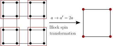
Figure 5: (Left) Illustration of the classical and the quantum lattice in two-dimensional real space (blue figure). The two lattices agree for the Langevin equation with white noise where ${s_{\Lambda}}=s_{\Lambda,\text{\tiny{max}}}$, see the left lattice sketch. Using a sharp regulator only field modes with $|p|\leq{s_{\Lambda}}$ receive a non-vanishing contribution from the colored noise term. This leads to a coarser quantum lattice (blue circles) compared to its classical counterpart (black points) which is unaffected by the cutoff.
(Right) A typical block spin transformation in two dimensions is illustrated (red figure). A possible choice of the transformation is to define the blocked field variables by averages over the four fields inside the red squares. This leads to a coarser lattice with double the lattice spacing and a quarter of the original lattice points. The illustrations point out the analogy between colored noise coarsening the quantum lattice and standard block spin transformations.

V Colored Noise and the Renormalization Group

Colored noise introduces a UV cutoff ${s_{\Lambda}}$. The change of the theory with an infinitesimal change of the cutoff is governed by the renormalization group. In terms of our lattice setup colored noise leads to the separation into the classical and the quantum lattice (18). The momentum space quantum lattice (19) contains only field modes with $|p|\leq{s_{\Lambda}}$. Those receive a non-zero contribution to fluctuations from the colored noise term in the Langevin equation (16). The remaining contribution encoded in the drift term is purely classical and applies to all field modes. Let $s_{\Lambda,\text{\tiny{max}}}$ denote the maximum cutoff on the lattice with $N^{d}$ points. In general, for a given cutoff ${s_{\Lambda}}\leq s_{\Lambda,\text{\tiny{max}}}$ the quantum lattice in momentum space has less points than the classical lattice. In the limit $\tau\to\infty$ the field modes with $|p|>{s_{\Lambda}}$ assume their classical value according to the limit of the gradient flow. The fewer points of the quantum momentum lattice translate into a coarser quantum real space lattice as compared to the classical real space lattice, see Fig. 5. With this in mind we study the relation of the colored noise Langevin evolution to the renormalization group in more detail. We investigate if the effect of the cutoff ${s_{\Lambda}}$ may be compensated by varying the lattice spacing $a$, thus tuning the coarseness of the quantum real space lattice (19). To this end we compare a simulation with white noise at ${s_{\Lambda}}=s_{\Lambda,\text{\tiny{max}}}$ on a coarse lattice with spacing $a_{1}$ with a colored noise simulation at cutoff ${s_{\Lambda}}<s_{\Lambda,\text{\tiny{max}}}$ on a fine lattice with spacing $a_{2}<a_{1}$.

Our procedure is to introduce scale factors for the following parameters

$$a\to a^{\prime}=s^{-1}a\,,\ N\to N^{\prime}=sN\,,p\to p^{\prime}=sp\,,$$ (34)

where $\ s\geq 1$ and $a$, $a^{\prime}$ are the original coarse and the fine lattice spacing. Correspondingly, the lattice size $N$ as well as the lattice momenta $p$ are transformed. The physical volume $(aN)^{d}$ is thereby kept constant. The cutoff is transformed according to

$${s_{\Lambda}}(a,N)\to{s_{\Lambda}}^{\prime}(a^{\prime},N^{\prime})=s^{-1}{s_{\Lambda}}(a^{\prime},N^{\prime})\,.$$ (35)

To give an explicit example of our transformation logic we consider the case $N=4$, $s=2$. Let the cutoff on the coarse lattice be ${s_{\Lambda}}(a,N=4)\equiv s_{\Lambda,\text{\tiny{max}}}(a,4)=2$. This corresponds to the white noise case. The transformed cutoff reads ${s_{\Lambda}}^{\prime}(s^{-1}a,sN)=2=s_{\Lambda,\text{\tiny{max}}}(a/2\,,8)\,/\,2$. This corresponds to a colored noise simulation at half the maximum cutoff on the finer lattice.

The above scaling transformations result in a change of the parameters $\kappa$ and $\lambda$ in the scalar theory introduced in Sec. IV. From now on we explicitly consider the two-dimensional theory. To derive the tree-level renormalization group equations for the parameters $\kappa$ and $\lambda$ we fix the bare parameters $m_{0},\,g_{0}$, see (22) in Sec. IV. The first expression of (34) yields

$$(am_{0})^{2} \to s^{-2}\,(am_{0})^{2}\,,$$

$$a^{2}g_{0} \to s^{-2}a^{2}g_{0}\,.$$ (36)

Next we use the definition (22) in (36) leading to

$$s^{-2}\left[\frac{1-2\lambda}{\kappa}-4\right] =\frac{1-2\lambda^{\prime}}{\kappa^{\prime}}-4$$

$$s^{-2}\frac{6\lambda}{\kappa^{2}} =\frac{6\lambda^{\prime}}{{\kappa^{\prime}}^{2}}\,.$$ (37)

These equations can be solved for $\kappa^{\prime}$ and $\lambda^{\prime}$ used in the colored noise simulation with cutoff ${s_{\Lambda}}^{\prime}$. We remark, that the equations (37) are akin with standard block-spinning equations. Under a complete block spin transformation the partition function is invariant. This requires an adjustment of the couplings of the theory which completes the renormalization group step. The right-hand side of Fig. 5 shows a typical block spin transformation on a two-dimensional lattice. Field variables are organized into blocks by local averaging which reduces the number of lattice points and renders the lattice coarser. The physical volume thereby remains fixed. For the correlation length this entails

$$2\,\xi(N^{\text{\tiny{B}}}=N/2,\kappa^{\text{\tiny{B}}},\lambda^{\text{\tiny{B}}})=\xi(N,\kappa,\lambda)\,,$$ (38)

where $N^{\text{\tiny{B}}},\kappa^{\text{\tiny{B}}},\lambda^{\text{\tiny{B}}}$ are the number of lattice points and the adjusted couplings on the blocked lattice. Our procedure is therefore analogous to block spinning since decreasing the cutoff ${s_{\Lambda}}$ generates the local averaging and the coarsening of the quantum lattice.

VI Numerical Results

In this section, we present numerical results for the scalar theory in two dimensions. All simulations in this work have been carried out using the sharp regulator function defined in (7) and a fixed Langevin time step $\Delta\tau=10^{-2}$. For a comparison of different regularization choices see App. D.2. In the first part of this section we study the effect of the sliding cutoff scale ${s_{\Lambda}}$ by means of the observables introduced in Sec. IV. Our simulation with maximal ${s_{\Lambda}}$ (white noise) reproduces the results in De et al. (2005). In the second part we focus on the relation between colored noise and the real space renormalization group.

VI.1 Colored Noise: incomplete blocking

A first check of our colored noise approach is shown in Fig. 6. The expectation value of the absolute magnetization measured on a $32\times 32$ lattice is plotted as a function of the cutoff ${s_{\Lambda}}$. Here, for the parameter choice ($\kappa=0.26$, $\lambda=0.02$) the classical theory is in the broken phase and the full quantum theory is in the symmetric phase. The white noise result (${s_{\Lambda}}=16$) is indicated by the blue dashed line. We find that colored noise (red data) allows for a consistent interpolation between the full quantum theory and the classical theory.

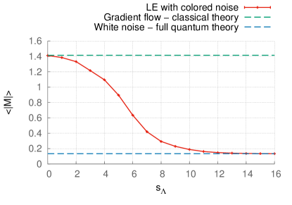
Figure 6: Magnetization $\langle|M|\rangle$ as a function of the cutoff ${s_{\Lambda}}$ for $\kappa=0.26$, $\lambda=0.02$ and $N=32$. For these external parameters $(\kappa,\lambda)$ the minima of the classical potential are located at $\pm\phi_{\text{\tiny{min}}}$ with $\phi_{\text{\tiny{min}}}=\sqrt{2}$ as given by (25). We find a consistent interpolation between the classical and the full quantum theory using our colored noise setup.

Next the interpolation between the two phases is investigated further by considering the fluctuation content of the theory. Thereto, we analyze the susceptibility, the Binder cumulant and the renormalized mass shown in Fig. 7. The parameters are the same as for Fig. 6. Cutting off ultraviolet modes gradually moves the susceptibility (left) and the Binder cumulant (middle) across the phase transition. This confirms the effects of colored noise observed in Fig. 6. The right plot in Fig. 7 shows the renormalized mass calculated from the second moment and the connected susceptibility. The mass decreases with lowering the cutoff which means that the correlation length (in lattice units) increases. Beyond the critical point we expect the renormalized mass to increase again. However, for ${s_{\Lambda}}<4$ the sharp regulator induces oscillations in the correlation function of time slices. Then, $m_{R}$ as defined in (33) shows a delayed transition from the symmetric to the broken phase. This problem can be resolved with the application of a smooth regulator function. In Appendix D.2 we analyze the behaviour of the correlation function of time slices comparing two different regularization choices. From this we can draw conclusions on the behaviour of $m_{R}$ for any ${s_{\Lambda}}$. In summary we find that the susceptibility, the Binder cumulant and the renormalized mass represent quantities that are sensitive to the application of colored noise if all bare parameters ($\kappa,\lambda$) and the lattice size $N$ are kept fixed.

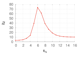
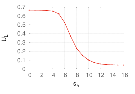
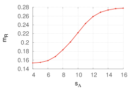
Figure 7: The phase transition of the theory is shown by means of its characteristic observables as a function of the cutoff ${s_{\Lambda}}$. The parameters $N=32,\kappa=0.26$ and $\lambda=0.02$ are fixed. (Left) The susceptibility shows a peak indicating that the quantum theory moves from the symmetric to the broken phase where the classical theory lives as ultraviolet modes are being removed successively. (Middle) The Binder cumulant confirms this effect of colored noise. (Right) The renormalized mass $m_{R}$ smoothly decreases towards the phase transition as the cutoff is lowered from ${s_{\Lambda}}=16$ to ${s_{\Lambda}}=4$. For ${s_{\Lambda}}<4$, $m_{R}$ as defined in (33) shows a delayed phase transition from the symmetric to the broken phase. Moreover, below ${s_{\Lambda}}=4$ the sharp cutoff imprints artifacts on the correlation function. For a detailed illustration of this behaviour see also Appendix D.2.

To continue our analysis we investigate the susceptibility as a function of $\kappa$ for different cutoffs ${s_{\Lambda}}$ as shown in Fig. 8. Here, the results were produced on a $64\times 64$ lattice where $\lambda=0.02$ is kept fixed. The violet curve depicts the white noise result. Our observations are: The peak position corresponding to $\kappa_{c}$ is successively shifted towards lower values of $\kappa$ with decreasing cutoff. This is consistent with the previous results in this section. Colored noise removes quantum fluctuations rendering the theory more classical. In the limit of the pure gradient flow the peak of the susceptibility would lie directly on the tree-level value of $\kappa_{c}^{(\text{cl})}=0.24$ according to (26). The stepwise UV regularized theory shows its critical behaviour in ranges of $\kappa$ where the full quantum theory (${s_{\Lambda}}=s_{\Lambda,\text{\tiny{max}}}$) lives in the symmetric phase.

Moreover, in the situations studied here the peak height shrinks when lowering the cutoff below ${s_{\Lambda}}=4$. This suggests that the momentum fluctuations below this characteristic momentum scale given by ${s_{\Lambda}}=4$ are relevant for the physics observed. Removing these momenta with a lower cutoff therefore modifies the theory. In turn, the momentum fluctuations above this scale are physically irrelevant.

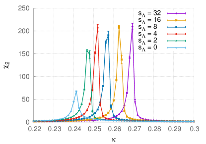
Figure 8: The susceptibility $\chi_{2}$ as a function of $\kappa$ for $N=64$ and fixed $\lambda=0.02$ for different cutoffs ${s_{\Lambda}}$. As the cutoff is lowered the peak of the susceptibility is being shifted towards smaller values of $\kappa$ and approaches the classical critical value $\kappa_{c}^{(\text{cl})}=0.24$. For the lowest cutoffs the peak height shrinks. Note that the white noise result is represented by the violet curve for $s_{\Lambda,\text{\tiny{max}}}=32$.

VI.2 Colored noise: complete blocking at tree level

In this section we relate the effects of colored noise to the real space renormalization group. Following the procedure outlined in Sec. V we set up the white noise reference simulation $(s=1,{s_{\Lambda}}=s_{\Lambda,\text{\tiny{max}}})$ on an $8\times 8$ lattice. The parameters are chosen to be $\lambda=\lambda^{(1)}=0.02$ and $0.22\leq\kappa=\kappa^{(1)}\leq 0.32$ with lattice spacing $a=a^{(1)}$. This determines the full quantum theory we want to compare our colored noise results with. We proceed by setting $s=2,4,8$ and perform colored noise simulations with finer lattice spacings $a^{(s)}$ on $N^{(s=2)}\times N^{(s=2)}=16\times 16$, $N^{(s=4)}\times N^{(s=4)}=32\times 32$ and $N^{(s=8)}\times N^{(s=8)}=64\times 64\,$ lattices at the corresponding cutoffs $s^{-1}\,s_{\Lambda,\text{\tiny{max}}}(a^{(s)},N^{(s)})$. Table 1 summarizes the lattice spacings $a^{(s)}$ and cutoffs ${s_{\Lambda}}$ used in the simulations. Accordingly, the transformed parameters are determined from (37). The resulting parameters $(\kappa^{(s)},\,\lambda^{(s)})$ are plotted in Fig. 9.

$N$	lattice spacing	${s_{\Lambda}}$	$\sqrt{d}\,(2\pi/a^{\tiny{(s)}}N)\,{s_{\Lambda}}$
$8$	$a^{(s=1)}=a$	$s_{\Lambda,\text{\tiny{max}}}=4$	$\sqrt{2}\frac{\pi}{a}$
$16$	$a^{(s=2)}$ = $a/2$	$s_{\Lambda,\text{\tiny{max}}}/2=4$	$\sqrt{8}\frac{\pi}{a}$
$32$	$a^{(s=4)}$ = $a/4$	$s_{\Lambda,\text{\tiny{max}}}/4=4$	$\sqrt{32}\frac{\pi}{a}$
$64$	$a^{(s=8)}$ = $a/8$	$s_{\Lambda,\text{\tiny{max}}}/8=4$	$\sqrt{128}\frac{\pi}{a}$

Table 1: Lattice scales for the RG transformation (36) in two dimensions. The last column shows the lattice cutoff with reinstated lattice spacing.

Fig. 10 shows the Gaussian fluctuations by means of the volume rescaled connected susceptibility $\chi_{2}/V$ plotted as a function of the untransformed hopping parameter $\kappa^{(1)}$ at fixed $\lambda^{(1)}=0.02$. That is we consider $(\chi_{2}/V)[\kappa^{(s)}(\kappa^{(1)},\lambda^{(1)}),\lambda^{(s)}(\kappa^{(1)},\lambda^{(1)})]$. Analogously, the Binder cumulant $U_{L}$ as well as the rescaled renormalized mass $Nm_{R}$ are presented in Fig. 11 and Fig. 12. The violet curve represents the full quantum theory produced on the $8\times 8$ lattice with white noise. We find that the colored noise results (blue for $N^{(s=2)}=16$, red for $N^{(s=4)}=32$ and dark yellow for $N^{(s=8)}=64$) are in close agreement with the results for the full theory. This meets the expectations of our construction. Although the classical lattices for different $s$ do not coincide in size, the quantum lattices are the same due to the rescaling (36). However, a few deviations are clearly visible.

The correlation function of time slices for the choice $\kappa^{(1)}=0.22,\lambda^{(1)}=0.02$ and the transformed parameters $\kappa^{(s)},\lambda^{(s)}$ thereof are shown in Fig. 13. The sharp regulator affects the colored noise correlators at small Euclidean times and causes oscillations for larger times as already mentioned in Sec. VI. However, the results seem to agree well if we rescale the Euclidean time axis for the $s=1,2,4$ cases to the time extent of the $N^{(s=8)}=64$ lattice. The shape of the correlator hints also the behaviour of the correlation length regardless of the artifacts from the sharp cutoff. In agreement with (38) we find that the correlation lengths in lattice units fulfill $\xi(N^{(s)},\kappa^{(s)},\lambda^{(s)})\approx s\,\xi(N,\kappa^{(1)},\lambda^{(1)})$. The correlation length increases which is consistent with the requirement $a\to a^{(s)}=a/s$. This is moreover in agreement with the concept of the block spin transformation (here in a kind of reverted sense) as discussed in Sec. V. Accordingly, from investigating the renormalized mass in Fig. 12 we find that $m_{R}(N,\kappa^{(1)},\lambda^{(1)})\approx s\,m_{R}(N^{(s)},\kappa^{(s)},\lambda^{(s)})$.

In Fig. 14 the order parameter $\langle|M|\rangle$ is plotted as a function of $\kappa^{(1)}$. The colored noise results seem to converge with increasing lattice size to the dark-yellow curve for $N^{(s=8)}=64$.

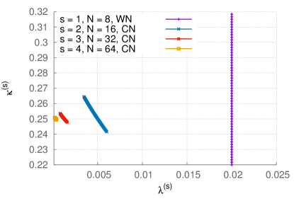
Figure 9: Transformed values for $\kappa^{(s)}$ and $\lambda^{(s)}$ used in simulations. The violet line represents the parameter range used for the $s=1$ white noise simulation.

There are several error sources that have to be taken into account. The deviations in the critical region are influenced by critical slowing down, see Fig. 10 and Fig. 12. The latter poses a hard issue for a local updating algorithm such as the Langevin equation. Furthermore, finite size effects are a possible error source for the mismatch of our data in the critical region. Those are also clearly visible in the order parameter in Fig. 14. Moreover, the deviations from the full quantum theory observed in our data indicate that our compensation procedure might be incomplete. One reason is that our naive renormalization group transformation is based on the tree-level relations (37). With increasing $s$ the deviation from the tree-level relations should increase as well due to the running of $m_{0}^{2}$ and $g_{0}$ affecting $\kappa$ and $\lambda$. A further reason is that the number of blocking steps is limited on a finite lattice. Here, only for the first RG step our procedure seems to yield correct results.

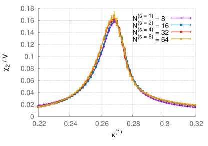
Figure 10: The connected two-point susceptibility rescaled by the volume as a function of $\kappa^{(1)}$ for different cutoff scales ${s_{\Lambda}}$. The violet curve represents the white noise reference result on the smallest and coarsest lattice. All of the remaining curves for $s=2,4,8$ were produced by means of colored noise with couplings adjusted according to the RG transformation (37).

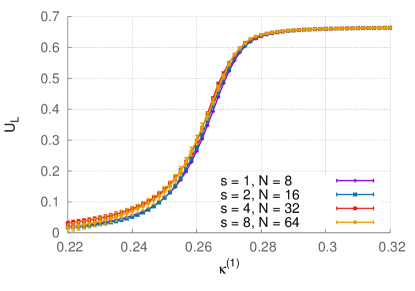
Figure 11: The Binder cumulant $U_{L}$ as a function of $\kappa^{(1)}$ for different cutoff scales ${s_{\Lambda}}$. The violet curve represents the white noise result.

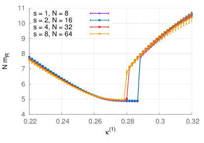
Figure 12: The rescaled renormalized mass $Nm_{R}$ as a function of $\kappa^{(1)}$ for different cutoff scales ${s_{\Lambda}}$. The violet curve represents the white noise result.

Figure 13: The correlation function of time slices $G_{c}(t)$ for different lattice sizes $N^{(s)}$ and transformed couplings $(\kappa^{(s)},\lambda^{(s)})$. The violet curve represents the white noise result.

Figure 14: The magnetization as a function of $\kappa^{(1)}$ for different cutoff scales ${s_{\Lambda}}$. The violet curve represents the white noise result.

Figure 15: The susceptibility rescaled by the volume as a function of $\kappa^{(1)}$ for different cutoffs ${s_{\Lambda}}$ on large lattices. The violet curve represents the white noise result.

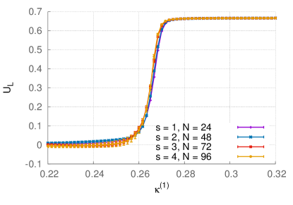
Figure 16: The Binder cumulant as a function of $\kappa^{(1)}$ for different cutoff scales ${s_{\Lambda}}$. The violet curve represents the white noise result.

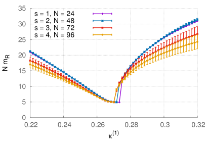
Figure 17: The rescaled renormalized mass $Nm_{R}$ as a function of $\kappa^{(1)}$ for different cutoff scales ${s_{\Lambda}}$. The violet curve represents the white noise result.

Figure 18: The magnetization as a function of $\kappa^{(1)}$ for different cutoff scales ${s_{\Lambda}}$. The violet curve represents the white noise result.

To cope with the finite size effects, we repeat our analysis considering larger lattices. We proceed analogously as before but in contrast to the discussion above we carry out the $s=1$ simulation using white noise on a larger $24\times 24$ lattice and set the scale factors for the colored noise simulations to $s=2,3,4$. The parameter set for the full theory is again given by $0\leq\kappa^{(1)}\leq 0.22$ and $\lambda^{(1)}=0.02$. Note, that the lattice sizes for the simulations with colored noise at half, third and quarter the maximum cutoff are now $N^{(s=2)}\times N^{(s=2)}=48\times 48$, $N^{(s=3)}\times N^{(s=3)}=72\times 72$ and $N^{(s=4)}\times N^{(s=4)}=96\times 96$.

From the susceptibility shown in Fig. 15 and the Binder cumulant in Fig. 16 we find that by halving the lattice spacing the results from the $N^{(s=1)}=24$ and the $N^{(s=2)}=48$ simulations are in good agreement. In the critical regime the results for larger lattices however deviate from the white noise reference result.

The renormalized mass in Fig. 17 shows that the $N^{(s=1)}=24$ and the $N^{(s=2)}=48$ data agree well over the whole range in the hopping parameter in spite of the deviation caused by the (remaining) finite size effect around the critical point. The larger lattices however, indicate that the masses differ from the white noise result. We remark that the simulations are plagued by a bad signal-to-noise ratio, visible in the correlator for parameters sufficiently far in the symmetric or broken phase respectively. The magnetization for the larger lattices in Fig. 18 shows an analogous behaviour as observed on the small lattices. We conclude, that except for the renormalized mass our renormalization procedure gives the same result on large and small lattices.

The results in this section have been produced from $10^{6}$ measurements of time slice configurations for each lattice size. Between two measurements we have performed 100 subsequent Langevin update sweeps corresponding to a Langevin time $\tau=1$ without measurement to reduce the autocorrelation of the observables. After a standard data blocking check we find that this is not enough, especially in the case of the large and fine lattices. The data is more severely correlated. For example at $\kappa^{(1)}=0.26$ for an $N=96$ lattice a block must have a minimum length of 5000 which we have used for a standard blocked Jackknife error analysis.

VII Cooling with colored noise - applications

In the previous sections we have shown that the cutoff can be decreased stepwise without changing the physics content of the theory if the cutoff is still sufficiently large. The complementary Wilsonian picture is that of integrating out degrees of freedom: with colored noise the path integral measure $P_{\Lambda}[\phi]$ only involves modes with $p^{2}\leq\Lambda^{2}$. Accordingly, let us consider the colored stochastic process (5), (6) with $S\to S_{{\rm eff},\Lambda}$, where the latter already contains the quantum effects of fields with $p^{2}>\Lambda^{2}$,

$$e^{-S_{{\rm eff},\Lambda}[\phi]}=\int d\phi_{p^{2}>\Lambda^{2}}\,e^{-S[\phi]}\,,$$ (39)

This leads us to

$$\frac{\partial\phi(x,\tau)}{\partial\tau}=-\frac{\delta S_{{\rm eff},\Lambda}}{\delta\phi(x,\tau)}+r_{\Lambda}(\Delta_{x})\,\eta(x,\tau)\,,$$ (40a)

with

$$\frac{\partial P_{{\rm eff},\Lambda}}{\partial\tau}=\int\mathrm{d}^{d}x\frac{\delta}{\delta\phi_{x}}\left(\frac{\delta S_{{\rm eff},\Lambda}}{\delta\phi_{x}}+\,r_{\Lambda}^{2}(\Delta_{x})\,\frac{\delta}{\delta\phi_{x}}\right)P_{{\rm eff},\Lambda}\,.$$ (40b)

The stochastic process (40) gives the full correlation functions for momenta $p^{2}\leq\Lambda^{2}$. The related generating functional is that of the full theory

$$Z=\int d\phi_{p^{2}\leq\Lambda^{2}}\,e^{-S_{{\rm eff},\Lambda}[\phi]}=\int d\phi\,e^{-S[\phi]}\,,$$ (41)

with the classical action $S[\phi]$ used in the original Langevin evolution. The Wilsonian effective action $S_{{\rm eff},\Lambda}$ can be also understood in terms of an improved or perfect lattice action if an additional block spinning transformation is applied.

Figure 19: Sketch of colored noise cooling. Each point on a horizontal line represents a pair of couplings $(\kappa,\lambda)$. The vertical axis denotes the cutoff scale $\Lambda$. The upper horizontal line depicts the white noise limit, and the curves constitute lines of constant physics. The couplings of UV-irrelevant operators are also generated during the RG flow. The corresponding axes are perpendicular to the plane in the plot, and are dropped.
For $\Lambda\gg\Lambda_{\text{\tiny{phys}}}$ we have $S_{\rm eff,\Lambda}=S[\kappa_{\Lambda},\lambda_{\Lambda}]$, see (42), depicted by the dark-red straight and dashed lines. Changing $\Lambda$ at fixed couplings effectively changes the physics content, see vertical black dashed line and also the observables in Fig. 7.
The scale $\Lambda_{\text{\tiny{phys}}}$ and the orange band denote the bound below which the action in the colored noise simulation must be described by the full quantum effective action.

In summary the following picture emerges: if the ultraviolet cutoff is asymptotically large, lowering the cutoff only changes the bare couplings $\kappa_{\Lambda},\lambda_{\Lambda}$ in the classical lattice action to accommodate the RG-running of the theory. Effectively this defines a scale $\Lambda_{\text{\tiny{phys}}}$, and for $\Lambda\gg\Lambda_{\text{\tiny{phys}}}$ the above statement holds. Higher order operators are suppressed by UV power counting with powers of $\Lambda_{\text{\tiny{phys}}}/\Lambda$ and can be safely dropped. This leads us to

$$S_{{\rm eff},\Lambda\gg\Lambda_{\text{\tiny{phys}}}}\simeq S[\kappa_{\Lambda},\lambda_{\Lambda}]\,,$$ (42)

see also Fig. 19. In turn, for small cutoffs, $\Lambda\lesssim\Lambda_{\text{\tiny{phys}}}$, physical fluctuations are removed from the lattice. Then, RG-transformations of the bare parameters in the classical lattice action do not suffice to keep the physics constant. Still, the latter can be achieved by RG transformations leading to improved or perfect actions,

$$S_{{\rm eff},\Lambda\lesssim\Lambda_{\text{\tiny{phys}}}}\neq S[\kappa_{\Lambda},\lambda_{\Lambda}]\,.$$ (43)

This idea is depicted in Fig. 19. It also suggests a systematic way to use the Wilsonian picture in terms of the (lattice) functional renormalization group (FRG) for improved lattice computations as well as for effectively determining $\Lambda_{\text{\tiny{phys}}}$. In contrast to the previous section we shall consider RG transformations beyond tree-level on lattices of fixed size and lattice spacing. These transformations are encoded in the flow equation for the Wilsonian effective action $S_{\rm eff,\Lambda}$. In the present work we concentrate on the sharp cutoff, a more general analysis also including smooth cutoffs will be presented elsewhere.

For the sharp cutoff $S_{\rm eff,\Lambda}$ satisfies the Wegner-Houghton equation Wegner and Houghton (1973). For the sake of computational convenience we formulate it for the 1PI effective action, the Legendre transform of $S_{\rm eff,\Lambda}$ (where the cutoff term is subtracted Berges et al. (2002); Polonyi (2003); Pawlowski (2007); Delamotte (2012); Rosten (2012); Metzner et al. (2012)),

$$\partial_{\Lambda}\Gamma_{\Lambda}[\bar{\phi}]=\frac{1}{2}{\text{Tr}}\langle\phi(p)\phi(-p)\rangle_{c}\,\Lambda^{2}\partial_{\Lambda}\left(\frac{1}{r_{\Lambda}(p^{2})}-1\right)\,,$$ (44)

where the subscript _c stands for the connected part of the two-point function similarly as introduced in Sec. IV. The trace Tr stands for the sum over momenta in the Brillouin zone, and $\bar{\phi}=\langle\phi\rangle$. In the continuum limit it turns into the standard momentum integration $\int d^{d}p/(2\pi)^{d}$. In (44) a suitable smoothing of the sharp cutoff is assumed and mandatory on the lattice. The propagator is the inverse of the second derivative of $\Gamma_{\Lambda}$ w.r.t. the fields, $\Gamma^{(2)}_{\Lambda}=\delta^{2}/\Gamma_{\Lambda}\delta\phi^{2}$, and hence (44) is a closed equation for $\Gamma_{\Lambda}$. In the continuum it takes the simple form

$$\Lambda\partial_{\Lambda}\Gamma_{\Lambda}[\bar{\phi}]=\frac{1}{2}{\text{Tr}}\log\left(\Gamma^{(2)}_{\Lambda}[\bar{\phi}]\right)(p^{2}=\Lambda^{2})\,.$$ (45)

In the UV regime with $\Lambda\gg\Lambda_{\text{\tiny{phys}}}$ the effective action is given by the classical action, see (42). Then the flow equation is a closed equation for $\kappa(t)$ and $\lambda(t)$ with $t=\log\Lambda/\Lambda_{\rm UV}$, where $\Lambda_{\rm UV}$ is a normalization scale, typically the initial UV scale. In the present case this is the maximal momentum on the classical lattice. Another convenient definition originates in $\Lambda/\Lambda_{\rm UV}=s_{\Lambda}/s_{\Lambda_{\rm UV}}$. Since $s_{\Lambda}$ is already dimensionless we drop the normalization and use

$$t=\log s_{\Lambda}\,.$$ (46)

For $\Lambda\lesssim\Lambda_{\text{\tiny{phys}}}$ the simple closed flows for $\kappa(t)$ and $\lambda(t)$ do not hold anymore, and the higher operators will be important. By comparing the full flows with the simplified ones the physical scale $\Lambda_{\text{\tiny{phys}}}$ can be defined as the scale below which the correlation functions computed from the stochastic processes with either $S$ and $S_{\rm eff}$ show significant deviations. Note that this procedure is less costly than the blocking procedure which involves decreasing the lattice spacing while simultaneously increasing the number of lattice points.

A full analysis of this framework goes beyond the scope of the present work. Here we want to provide some first simple practical computations that also give indications of the precision needed in fully quantitative analyses. To that end we approximate the lattice RG transformations by the functional RG flow equations in the continuum theory (45). In the asymptotic UV regime with $\Lambda\gg\Lambda_{\text{\tiny{phys}}}$ the effective action $\Gamma_{\Lambda}$ is given by the classical action, to wit

$$\Gamma_{\Lambda}[\phi]\simeq\int d^{d}x\left\{\frac{1}{2}\phi\left(-\partial^{2}+m^{2}\right)\phi+\frac{g}{4!}\phi^{4}\right\}\,,$$ (47)

for $m^{2}\geq 0$. Taking two and four field derivatives at $\phi=0$ and $p=0$ we are lead to the flows

$$\partial_{\Lambda}m=F_{m}(m,g)\,,\qquad\partial_{\Lambda}g=F_{g}(m,g)\,,$$ (48)

for the mass and the coupling. The latter can be converted to flows for the dimensionless lattice parameters $\kappa,\lambda$ using the relations (22). Note that the flow of $g$ runs like $1/\Lambda^{2}$ for large $\Lambda$ up to logarithmic corrections. Hence, at leading order only $m^{2}$ and $\kappa$ run logarithmically proportional to $\log(\Lambda)$ and $1/\log(\Lambda)$ for large $\Lambda$. Accordingly, for $\Lambda\to 1/2\Lambda$ the mass squared shifts by an amount proportional to $\log(2)$. The prefactor can be computed from (48). In explicit form, the dimensionful continuum flow equations for the mass $m$ and the coupling $g$ read

$$\Lambda\,\partial_{\Lambda}m^{2}=-\frac{g}{4\pi}\frac{1}{1+m^{2}/\Lambda^{2}}\,,$$ (49)

and

$$\Lambda\,\partial_{\Lambda}g=\frac{3}{4\pi}\,\frac{g^{2}}{\Lambda^{2}}\,\frac{1}{(1+m^{2}/\Lambda^{2})^{2}}\,.$$ (50)

The flow equations are cast into dimensionless form by multiplying both sides with the fixed square lattice spacing $a^{2}$. The dimensionless cutoff reads $a\,\Lambda$ and the flow time is defined by $t:=\log(a\,\Lambda)$. Using the relations (22) leads to the flow equations for the lattice parameters.

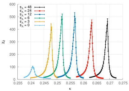
Figure 20: Susceptibility $\chi_{2}$ as a function of the hopping parameter $\kappa$ for different cutoffs ${s_{\Lambda}}$. The coupling is fixed to $\lambda=0.02$. The results shown here have been computed using a $96\times 96$ lattice. The white noise result corresponds to ${s_{\Lambda}}=48$.

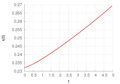
Figure 21: Scale dependence of the hopping parameter $\kappa$ from integrating the flow (51).

Figure 22: Predictions for the critical hopping parameter $\kappa_{c}$ from the functional RG flow equations (blue) in comparison with colored noise simulations on the lattice (red).

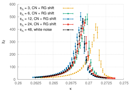
Figure 23: Shift of the susceptibility peaks according to the results for $\kappa$ and $\lambda$ from the flow equations (51) and (52).

$$\partial_{t}\,\kappa(t)\,=\, \frac{3}{2}\frac{\lambda(t)}{\pi}\,\kappa(t)\,\frac{e^{2t}}{1+2\lambda(t)}$$

$$\times\frac{\kappa(t)\left(e^{2t}-4\right)-8\lambda(t)+1}{\left[\kappa(t)\left(e^{2t}-4\right)-2\lambda(t)+1\right]^{2}}\,,$$ (51)

$$\partial_{t}\,\lambda(t)\,=\, \frac{3}{2}\,\frac{\lambda(t)^{2}}{\pi}\,\frac{e^{2t}}{1+2\lambda(t)}$$

$$\times\frac{2\,\kappa(t)\left(e^{2t}-4\right)-10\lambda(t)+5}{\left[\kappa(t)\,\left(e^{2t}-4\right)-2\lambda(t)+1\right]^{2}}\,.$$ (52)

For a quantitative comparison between the continuum RG and colored noise cooling on the lattice we consider the peak positions $\kappa_{c}$ of the susceptibilities for different ${s_{\Lambda}}$ as shown in Fig. 20. The data stems from simulations on a $96\times 96$ lattice. The coupling $\lambda=0.02$ is fixed as in the previous sections. For the comparison we take into account the data for ${s_{\Lambda}}=3,6,12,24,48$. The flow equations (51) and (52) are initialized at the maximum flow time $t_{\text{max}}=\log(a\,\Lambda_{\text{max}})$ using the parameters $\lambda(t_{\text{max}})=0.02$ and $\kappa(t_{\text{max}})=\kappa_{c,\text{WN}}$. Here, $\kappa_{c,\text{WN}}$ indicates the critical hopping parameter obtained from the simulation with white noise ($s_{\Lambda,\text{\tiny{max}}}=48$). Moreover, the continuum cutoff translates into its lattice counterpart with $a\,\Lambda_{\text{max}}=\sqrt{2}\pi\,C$, where $C$ is a free RG-parameter. The running hopping parameter $\kappa(t)$ is depicted in Fig. 21. To compute the remaining critical hopping parameters $\kappa_{c}$ from the RG flow corresponding to lower values of ${s_{\Lambda}}$ we evaluate $\kappa(t)$ at scales $t_{\text{max}}-n\,\log(2)$, where $n=1,2,3,4$. The red data points in Fig. 22 show the critical values $\kappa_{c}$ as a function of ${s_{\Lambda}}$ from the lattice simulations. The blue points denote the values of $\kappa_{c}$ obtained from the RG flow (51).

We find that at large cutoff scales the critical values $\kappa_{c}$ measured on the lattice coincide with those calculated from the flow equations. In contrast, for small cutoff momenta a deviation is visible. This indicates that at lower momentum scales the stochastic process in terms of the classical action fails to describe the full theory. There the classical action needs to be replaced by an effective action as mentioned above. We conclude that for the model considered in this work colored noise cooling is applicable at scales between the UV and a specific IR scale. In the case investigated here this IR scale lies between $s_{\Lambda,\text{\tiny{max}}}/4$ and $s_{\Lambda,\text{\tiny{max}}}/8$. This is also supported by the shifted susceptibility in Fig. 23 . Here, the peaks have been translated by the difference between $\kappa_{c,\text{WN}}$ and the values of $\kappa_{c}$ from the RG prediction, see Fig. 22. While the agreement between the curves is quite good up to ${s_{\Lambda}}=12$ (blue curve), for lower cutoffs the results deviate from the full theory, see the green and yellow curves.

There are a few caveats to mention. Firstly, we work at fixed $\lambda$ in our lattice simulations. When lowering ${s_{\Lambda}}$, $\lambda$ should be adjusted properly. Secondly, we approximate RG transformations of the lattice parameters by the continuum functional RG. For a more exact comparison between the RG transformations and the lattice results, we need to solve the flow equations (49) and (50) on the lattice. This however comes with a few technical complications since the flow is only defined at the discrete lattice momenta.

VIII Conclusions and outlook

In this work we have investigated lattice theories with Stochastic Quantization with UV-regularized colored noise. Cooling the Langevin evolution by removing field configurations in the UV may be a promising candidate to optimize lattice simulations of systems with a clear scale separation between the relevant physics and the asymptotic UV regime. There are two possible interpretations of our method. The first is that the colored noise LE can be applied in the traditional sense of smoothing out UV-fluctuations. The alternative interpretation is to sample smooth configurations directly from the UV-regularized Langevin evolution.

Here we have exploited the latter interpretation which also can be connected directly to the renormalization group. The scale of the smooth fields is set by using an external cutoff parameter $\Lambda$. By varying $\Lambda$ the colored noise Langevin equation interpolates between the full quantum theory accessible in a standard white noise simulation and the classical theory.

Our approach has been put to work within a real scalar field theory in two dimensions using a sharp momentum cutoff. We have shown, that for sufficiently large cutoff scales $\Lambda$ no relevant physics is cut off. In Sec. VII we have analyzed the viability of the colored noise cooling by sampling configurations with colored noise on lattices of fixed size. Thereby the form of the classical action is kept unchanged. This procedure is only valid for $\Lambda\gg\Lambda_{\text{\tiny{phys}}}$. In turn, for $\Lambda\lesssim\Lambda_{\text{\tiny{phys}}}$ deviations grow large. At this point a description by means of an effective action might be necessary. Furthermore finite size and volume effects on the lattice certainly also play a r$\hat{\rm o}$le and prohibit the use of the continuum approximation for small UV cutoffs. Hence, a refined analysis may even lower the cooling range.

Even without the refined analysis we have shown that a remarkably large regime of ultraviolet fluctuations can be removed without altering the physics content of the theory. The next step is to probe the maximal colored cooling by identifying the lowest possible cutoff scale at which the use of the classical action is still valid. Thereto, we compute the parameters $\kappa$ and $\lambda$ from the associated RG flows at a desired scale $\Lambda$ and use them in the lattice simulation. This is current work in progress.

Moreover, in our ongoing work we use a (Symanzik) improved action and study the flow of the couplings of operators with dimension larger than $O(a^{2})$. Further perspectives of the method are to explore the effects of regulator functions different from the sharp cutoff beyond the effects shown in Appendix D.2.

Applications of the method to SU(N) gauge theories and to finite density models are also work in progress. In theories with a complex action induced e.g. by a finite chemical potential, the Complex Langevin evolution might be optimized by colored noise cooling.

Appendix A Fourier transformation on the Lattice

On the lattice the discrete Fourier transformation  of the field $\phi(x)$ reads

$$\phi(p)=\sum_{x}a^{d}\,\mathrm{e}^{-ip\cdot x}\phi(x)\,,$$ (53)

where the momenta $p$ are elements of the discrete Brillouin zone. The inverse Fourier transform of the field $\phi(x)$ is correspondingly given by

$$\phi(x)=\frac{1}{a^{d}\,N^{\tiny{d}}}\,\sum_{p}\,\mathrm{e}^{ip\cdot x}\,\phi(p)\,,$$ (54)

where the sum runs over all momenta in the Brillouin zone. In the thermodynamic limit $N\to\infty$ the previous equation converges to

$$\phi(x)=\frac{1}{(2\pi)^{d}}\int_{-\pi/a}^{\pi/a}\,\mathrm{d}^{d}p\,\mathrm{e}^{ip\cdot x}\,\phi(p)\,.$$ (55)

For the remaining part of this section we work in the thermodynamic limit.

The $O(a^{2})$ discretized Euclidean Laplace operator has the form

$$\Delta_{x,y}=-\frac{1}{a^{2}}\sum_{\mu=1}^{d}\,(\delta_{x+\hat{\mu},y}-2\,\delta_{x,y}+\delta_{x-\hat{\mu},y})\,.$$ (56)

Let $\Delta^{-1}_{x,y}$ denote the inverse lattice Laplacian obeying

$$\Delta_{x,y}\Delta^{-1}_{y,z}=\frac{\delta_{x,z}}{a^{d}}\,.$$ (57)

Substituting the Fourier transform of the Laplacian according to (55) in the previous equation yields

$$\quad\ \Delta_{x,y}\left[\frac{1}{(2\pi)^{d}}\int_{-\pi/a}^{\pi/a}\,\mathrm{d}^{d}p\,\mathrm{e}^{ip\cdot(y-z)}\,\Delta^{-1}(p)\right]$$

$$=\frac{1}{(2\pi)^{d}}\int_{-\pi/a}^{\pi/a}\,\mathrm{d}^{d}p\,\mathrm{e}^{ip\cdot(x-z)}\,.$$ (58)

Evaluating this further leads to the lattice Laplacian in momentum space

$$\Delta(p)=\frac{4}{a^{2}}\sum_{\mu=1}^{d}\sin^{2}\left(\frac{ap_{\mu}}{2}\right)\,.$$ (59)

The right-hand side of (59) appears in a similar fashion in the free propagator of a scalar field theory. It relates the physical momenta to the lattice momenta (14) by

$$\tilde{p}_{\mu}:=\frac{2}{a}\sin\left(\frac{a\,p_{\mu}}{2}\right).$$ (60)

Appendix B Observables

In this section we work in lattice units. Let $V=N_{s}^{d-1}$ denote the spatial lattice volume and $T=N_{t}$ the time extent of the lattice. Similarly as above we work with $N_{s}=N=N_{t}$. The total lattice volume is $\Omega=VT$. In the following we derive in more detail a few of the key observables of a real scalar field theory with the lattice action given in (21). We keep our notation close to Montvay and Münster (1997). The connected two-point susceptibility is defined as the integrated connected two-point correlation function (28). It can be formulated in terms of the magnetization $M$ defined in (27) using that $\langle\phi(x)\rangle=\langle\phi(0)\rangle=\langle M\rangle$.

$$\chi_{2} :=\sum_{x}G_{c}(x,0)=\sum_{x}\langle\phi(x)\phi(0)\rangle_{c}$$

$$=\sum_{x}\left(\langle\phi(x)\phi(0)\rangle-\langle\phi(x)\rangle\langle\phi(0)\rangle\right)$$

$$=\sum_{x}\left(\frac{1}{\Omega}\,\left\langle\sum_{y}\phi(x+y)\phi(y)\right\rangle-\langle M\rangle^{2}\right)$$

$$=\frac{1}{\Omega}\,\left\langle\sum_{x,y}\phi(x+y)\phi(y)\right\rangle-\Omega\,\langle M\rangle^{2}$$

$$=\left\langle\sum_{y}M\phi(y)\right\rangle-\Omega\,\langle M\rangle^{2}$$

$$=\Omega\,(\langle M^{2}\rangle-\langle M\rangle^{2})=\Omega\,\langle M^{2}\rangle_{c}\,.$$ (61)

In the step from the third to the fourth as well as from the fifth to the sixth equation translation invariance on the lattice has been used. Moreover, we exploited the linearity of the (path integral) expectation value. Alternatively, the connected susceptibility is just the Fourier transform of the connected correlation function with momentum set to zero

$$\chi_{2}\equiv\left.\vphantom{\frac{dummy}{dummy}}\tilde{G}(p)\right|_{p=0}\,.$$ (62)

Here, the momentum space correlator for small $p$ has the form

$$\tilde{G}(p)=\frac{1}{2\kappa}\frac{Z_{R}}{m_{R}^{2}+p^{2}+O(p^{4})}\,.$$ (63)

From this, the second moment is determined according to

$$\mu_{2}\equiv-\left.\frac{\partial^{2}}{\partial p_{\nu}\partial p_{\nu}}\tilde{G}(p)\right|_{p=0}\,.$$ (64)

Explicitly, for the susceptibility it holds

$$\chi_{2}=\tilde{G}(0)=\frac{1}{2\kappa}\frac{Z_{R}}{m_{R}^{2}}\,.$$ (65)

The evaluation of (64) for the second moment yields

$$\mu_{2}=\frac{2d}{2\kappa}\frac{Z_{R}}{m_{R}^{4}}\,.$$ (66)

Thus, the renormalized mass is given by

$$m_{R}^{2}=2d\frac{\chi_{2}}{\mu_{2}}\,.$$ (67)

Next, we define the time slice as the spatial average of the field over the lattice at each time $t$

$$S(t)=\frac{1}{V}\sum_{\vec{x}}\phi(\vec{x},t)\,.$$ (68)

In a similar way as discussed above, we can express $\chi_{2}$ in terms of the integrated correlation function of time slices using $\langle S(t)\rangle=\langle S(0)\rangle=\langle M\rangle$.

$$\chi_{2}=\frac{1}{\Omega}\sum_{x,y}\langle\phi(x+y)\phi(y)\rangle-\Omega\langle M\rangle^{2}$$

$$=\frac{1}{\Omega}\sum_{(t,\vec{x}),(t^{\prime},\vec{y})}\langle\phi(\vec{x}+\vec{y},t+t^{\prime})\phi(\vec{y},t^{\prime})\rangle-\Omega\langle M\rangle^{2}$$

$$=\sum_{t,t^{\prime}}\,\frac{V}{T}\langle S(t+t^{\prime})S(t^{\prime})\rangle-V\sum_{t}\langle S(t)\rangle\langle S(0)\rangle$$

$$=V\,\sum_{t}\langle S(t)S(0)\rangle_{c}=V\,\sum_{t}G_{c}(t)\,.$$ (69)

The second moment $\mu_{2}$ can be expressed in form of time slices exploiting $\langle\phi(\vec{x},t)\rangle=\langle S(t)\rangle$ as follows

$$\mu_{2}=\sum_{x}x^{2}G_{c}(x,0)=\sum_{x}x^{2}\langle\phi(x)\phi(0)\rangle_{c}$$

$$=\sum_{\tiny{t,\vec{x}}}(t^{2}+{\vec{x}}^{2})\langle\phi(\vec{x},t)\phi(0,0)\rangle_{c}$$

$$=d\,\sum_{\tiny{t,\vec{x}}}t^{2}\langle\phi(\vec{x},t)\phi(0,0)\rangle_{c}$$

$$=d\,\sum_{\tiny{t,\vec{x}}}\,t^{2}\langle\phi(\vec{x},t)\phi(0,0)\rangle-d\,\sum_{\tiny{t,\vec{x}}}\,t^{2}\langle\phi(\vec{x},t)\rangle^{2}$$

$$=d\,\sum_{\tiny{t,\vec{x}}}t^{2}\langle\phi(\vec{x},t)S(0)\rangle-d\,\sum_{\tiny{t,\vec{x}}}\,t^{2}\langle S(t)\rangle^{2}$$

$$=d\,V\,\sum_{\tiny{t}}t^{2}\langle S(t)S(0)\rangle-d\,V\sum_{\tiny{t}}\,t^{2}\langle S(t)\rangle^{2}$$

$$=d\,V\sum_{\tiny{t}}t^{2}\langle S(t)S(0)\rangle_{c}\,.$$ (70)

In the step from the third to the fourth equation we have used the above premise that there is no distinguished direction on the lattice.

The corresponding formulae for a scalar field theory in $d=2$ read

$$\chi_{2} =\frac{1}{N^{2}}\sum_{x,y}\langle\phi(x+y)\phi(y)\rangle_{c}=N^{2}\langle M^{2}\rangle_{c}$$

$$=\sum_{t,t^{\prime}}\langle S(t+t^{\prime})S(t^{\prime})\rangle_{c}=N\sum_{t}\langle S(t)S(0)\rangle_{c}\,,$$ (71)

where

$$S(t)=\frac{1}{N}\sum_{x}\phi(x,t)$$ (72)

and

$$M=\frac{1}{N^{2}}\sum_{x}\phi(x)\,.$$ (73)

For the second moment we find

$$\mu_{2}=2N\sum_{t}t^{2}\langle S(t)S(0)\rangle_{c}\,.$$ (74)

Finally, the renormalized mass can be computed from

$$m_{R}=\left(\frac{4\chi_{2}}{\mu_{2}}\right)^{1/2}\,.$$ (75)

Appendix C Spacetime correlation function of colored noise

First, the spatial Fourier transform of the noise field $\eta(x,\tau)$ is given by

$$\eta(p,\tau)=\int\mathrm{d}^{d}x\,\eta(x,\tau)\,\mathrm{e}^{-ip\cdot x}\,.$$ (76)

The white noise correlation function in momentum space is obtained by applying the second relation from (3)

$$\langle\eta(p,\tau)\eta(q,\tau^{\prime})\rangle=2\,(2\pi)^{d}\,\delta^{(d)}(p+q)\,\delta(\tau-\tau^{\prime})\,.$$ (77)

In the continuum colored noise is defined by the convolution with the sharp regulator function (7)

$$\eta(x,\tau)_{\text{col}}=\frac{1}{(2\pi)^{d}}\int\,\mathrm{d}^{d}p\,\eta(p,\tau)\theta(\Lambda^{2}-p^{2})\,\mathrm{e}^{ip\cdot x}\,.$$ (78)

The correlation function for the colored noise field in $d$ dimensions is derived in the following.

$$\langle\eta_{\text{col}}(x,\tau)\,\eta_{\text{col}}(y,\tau^{\prime})\rangle$$

$$=\left\langle\frac{1}{(2\pi)^{2d}}\int\mathrm{d}^{d}p\,\mathrm{d}^{d}q\,\mathrm{e}^{-ip\cdot x}\mathrm{e}^{-iq\cdot y}\right.$$

$$\ \ \left.\vphantom{\frac{dummy}{dummy}}\times\theta(\Lambda-|p|)\theta(\Lambda-|q|)\,\eta(p,\tau)\eta(q,\tau^{\prime})\right\rangle$$ (79)

$$=\frac{2}{(2\pi)^{d}}\int\mathrm{d}^{d}p\,\mathrm{d}^{d}q\,\mathrm{e}^{-ip\cdot x}\mathrm{e}^{-iq\cdot y}\,$$

$$\quad\times\theta(\Lambda-|p|)\theta(\Lambda-|q|)\,\delta^{(d)}(p+q)\delta(\tau-\tau^{\prime})$$ (80)

$$=\frac{2}{(2\pi)^{d}}\,\int\,\mathrm{d}^{d}p\,\mathrm{e}^{-ip\cdot(x-y)}\theta(|\Lambda|-|p|)\,\delta(\tau-\tau^{\prime})\,$$ (81)

$$=\frac{2}{(2\pi)^{d}}\int_{0}^{\Lambda}\,\mathrm{d}|p||p|^{d-1}\int_{\vartheta_{d-1}=0}^{2\pi}\int_{\vartheta_{d-2}=0}^{\pi}\ldots\int_{\vartheta_{1}=0}^{\pi}$$

$$\quad\times\mathrm{e}^{{-i|p||x-y|\cos(\vartheta_{d-2})}}\,\sin^{d-2}(\vartheta_{1})\ldots\sin(\vartheta_{d-2})\,$$

$$\quad\times\mathrm{d}\vartheta_{1}\ldots\mathrm{d}\vartheta_{d-2}\,\mathrm{d}\vartheta_{d-1}\,\delta(\tau-\tau^{\prime})$$ (82)

$$=\frac{2}{(2\pi)^{d}}\int_{0}^{\Lambda}\,\mathrm{d}|p||p|^{d-1}\frac{\sin(|p||x-y|)}{|x-y|}\,\int\,\Omega_{d}\,\delta(\tau-\tau^{\prime})$$ (83)

$$=\frac{1}{2^{d-2}\pi^{d/2}\,\Gamma(\frac{d}{2})}\int_{0}^{\Lambda}\,\mathrm{d}|p||p|^{d-1}J_{0}(|p||x-y|)\,\delta(\tau-\tau^{\prime})\,.$$ (84)

Here $\Gamma(t):=\int\mathrm{d}y\,\mathrm{e}^{-y}y^{t-1}$ denotes the Euler gamma function and $J_{0}(x)\equiv\sin(x)/x$ is a Bessel function of the first kind. The Bessel profile is also visible in observables such as the correlation function of time slices for sufficiently low cutoff in numerical simulations. This is discussed further in Appendix D.2.

Appendix D Aspects of Stochastic Quantization with colored noise

D.1 Fokker-Planck equation

In this section, we derive the Fokker-Planck equation (FPE) with a noise kernel (6) which describes the evolution of the probability distribution $P(\phi,\tau)$ in fictitious time $\tau$. The derivation presented in Damgaard and Huffel (1987); Bern et al. (1987) is worked out in more detail focusing on the important technical steps. Thereto, we consider a real one-component interacting scalar field theory in $d$ dimensions whose Euclidean action reads

$$S=\int\mathrm{d}^{d}x\,\left[\frac{1}{2}\left(\sum_{\mu=1}^{d}(\partial_{\mu}\phi(x))^{2}\right)\vphantom{\sum_{\mu=1}^{d}}+\frac{m^{2}}{2}\phi^{2}(x)+V(\phi)\right]\,.$$ (85)

The regularized Langevin equation reads

$$\frac{\partial\phi(x,\tau)}{\partial\tau}=-\frac{\delta S}{\delta\phi(x,\tau)}+r_{\Lambda}(\Delta_{x})\,\eta(x,\tau)\,,$$ (86)

where $r_{\Lambda}(\Delta_{x})$ denotes the regularization function which depends on the cutoff parameter $\Lambda$ and the Laplacian $\Delta_{x}$ with $r_{\Lambda}(\Delta_{x})\to 1$ in the limit $\Lambda\to\infty$. The field is evolved in Langevin time according to

$$\phi(x,\tau)= \,\int_{x^{\prime}}\,\int_{-\infty}^{\tau}\mathrm{d}\tau^{\prime}\,G(x-x^{\prime},\tau-\tau^{\prime})$$

$$\hskip 8.5359pt\times\left[r_{\Lambda}(\Delta_{x})\,\eta(x,\tau^{\prime})-\frac{\delta V}{\delta\phi}\phi(x^{\prime},\tau)\right]\,,$$ (87)

where the Langevin Green’s function, see Damgaard and Huffel (1987) for the derivation, is given by

$$G(x-x^{\prime},\tau-\tau^{\prime})=\\ \theta(\tau-\tau^{\prime})\int_{p}\mathrm{e}^{-ip\cdot(x-x^{\prime})}\mathrm{e}^{-(\tau-\tau^{\prime})(p^{2}+m^{2})}\,.$$ (88)

Note, that the lower bound in the fictitious time integral is set to $-\infty$ such that at finite (positive) Langevin times the system is in thermal equilibrium. Stochastic averages are equivalent to functional averages over a probability distribution $P(\phi,\tau)$. Moreover, let $F[\phi]$ be an arbitrary functional of the field variables. To stress the explicit noise dependence of the field obtained as a solution of the Langevin equation we write $\phi_{\eta}$. Stochastic averages are written as

$$\langle F[\phi_{\eta}]\rangle_{\eta}= \,\int\,\mathcal{D}\eta\,F[\phi_{\eta}]\,\mathrm{exp}\left[-\frac{1}{4}\int\mathrm{d}\tau\mathrm{d}^{d}x\,\eta^{2}(x,\tau)\right]$$

$$= \int\mathcal{D}\phi\,F[\phi]\,P(\phi,\tau)\,.$$ (89)

Before we proceed, we derive some useful identities. First, it follows from (87)

$$\frac{\delta\phi(x,\tau)}{\eta(y,\tau)} =\theta(0)\int_{x^{\prime}}r_{\Lambda}(\Delta_{x})\,\delta^{(d)}(x-y)\int_{p}\mathrm{e}^{-ip\cdot(x-x^{\prime})}$$

$$=\frac{1}{2}\,r_{\Lambda}(\Delta_{x})\,\delta^{(d)}(x-y)\,,$$ (90)

where the convention $\theta(0)=\frac{1}{2}$ is used. Finally, we note the trivial identity

$$\left(2\frac{\delta}{\delta\eta_{y,\tau}}+\eta_{y,\tau}\right)\,\exp\left[-\frac{1}{4}\int_{\tau}\,\int_{x}\,\eta^{2}_{x,\tau}\right]=0\,.$$ (91)

To derive the FPE we consider the derivative with respect to fictitious time $\tau$ of the stochastic average given in (89). For simplicity, we drop the subscript $\eta$.

$$\frac{d}{d\tau}\langle F[\phi]\rangle=\,\left\langle\int_{x}\,\frac{\delta F[\phi]}{\delta\phi_{x,\tau}}\frac{\partial\phi_{x,\tau}}{\partial\tau}\right\rangle$$

$$=\left\langle\int_{x}\,\frac{\delta F[\phi]}{\delta\phi_{x,\tau}}\left(-\frac{\delta S}{\delta\phi_{x,\tau}}+r_{\Lambda}(\Delta_{x})\,\eta_{x,\tau}\right)\right\rangle$$

$$=\int\mathcal{D}\eta\left\{\,\int_{x}\,\frac{\delta F[\phi]}{\delta\phi_{x,\tau}}\left(-\frac{\delta S}{\delta\phi_{x,\tau}}+r_{\Lambda}(\Delta_{x})\,\eta_{x,\tau}\right)\right.$$

$$\quad\left.\times\mathrm{exp}\left[-\frac{1}{4}\int_{\tau}\,\int_{z}\,\eta^{2}_{z,\tau}\right]\right\}$$

$$=\,\int\mathcal{D}\eta\,\int_{x}\,\frac{\delta F[\phi]}{\delta\phi_{x,\tau}}$$

$$\quad\times\left(-\frac{\delta S}{\delta\phi_{x,\tau}}-2\int_{y}\,r_{\Lambda}(\Delta_{x})\,\delta^{(d)}(x-y)\,\frac{\delta}{\delta\eta_{y,\tau}}\right)$$

$$\quad\times\mathrm{exp}\left[-\frac{1}{4}\int\,\mathrm{d}\tau\,\mathrm{d}^{d}z\,\eta^{2}_{z,\tau}\right]\,.$$ (92)

In the second equation the Langevin equation (86) was inserted. The third equation follows by writing the noise average in the functional integral form. In the fourth equation the identity for the functional derivative with respect to the noise field from (91) was used. This can be simplified further as follows

$$\frac{d}{d\tau}\langle F[\phi]\rangle =\int\mathcal{D}\eta\,\mathrm{exp}\left[-\frac{1}{4}\int_{\tau}\,\int_{z}\eta^{2}_{z,\tau}\right]\,\int_{x}\,\left(-\frac{\delta S}{\delta\phi_{x,\tau}}+2\int_{y}\,r_{\Lambda}(\Delta_{x})\,\delta^{(d)}(x-y)\,\frac{\delta}{\delta\eta_{y,\tau}}\right)\,\frac{\delta F[\phi]}{\delta\phi_{x,\tau}}$$

$$=\left\langle\int_{x}\,\left(-\frac{\delta S}{\delta\phi_{x,\tau}}+2\int_{y}\,r_{\Lambda}(\Delta_{x})\,\delta^{(d)}(x-y)\,\frac{\delta}{\delta\eta_{y,\tau}}\right)\,\frac{\delta F[\phi]}{\delta\phi_{x,\tau}}\right\rangle$$

$$=\left\langle\int_{x}\left(-\frac{\delta S}{\delta\phi_{x,\tau}}+2\int_{y}\,r_{\Lambda}(\Delta_{x})\,\delta^{(d)}(x-y)\,\int_{w}\,\frac{\delta\phi_{w,\tau}}{\delta\eta_{y,\tau}}\frac{\delta}{\delta\phi_{w,\tau}}\right)\frac{\delta F[\phi]}{\delta\phi_{x,\tau}}\right\rangle$$

$$=\left\langle\int_{x}\left(-\frac{\delta S}{\delta\phi_{x,\tau}}+r^{2}_{\Lambda}(\Delta_{x})\,\frac{\delta}{\delta\phi_{x,\tau}}\right)\frac{\delta F[\phi]}{\delta\phi_{x,\tau}}\right\rangle.$$ (93)

Here, the first equation follows from an integration by parts with respect to $\eta$. The third equation uses the chain rule to calculate the functional derivative of $F$ with respect to $\eta$. The last equation is obtained by using the identity for the functional derivative of the field $\phi$ with respect to $\eta$ from (90). Moreover, it follows

$$\frac{d}{d\tau}\langle F[\phi]\rangle =\int\mathcal{D}\phi\,F[\phi]\frac{\partial P(\phi,\tau)}{\partial\tau}=\int\mathcal{D}\phi\,\left[\int_{x}\left(-\frac{\delta S}{\delta\phi_{x}}+r^{2}_{\Lambda}(\Delta_{x})\,\frac{\delta}{\delta\phi_{x}}\right)\frac{\delta F[\phi]}{\delta\phi_{x}}\right]P(\phi,\tau)$$

$$=\int\mathcal{D}\phi\,F[\phi]\int_{x}\,\frac{\delta}{\delta\phi_{x}}\left(\frac{\delta S}{\delta\phi_{x}}+r^{2}_{\Lambda}(\Delta_{x})\,\frac{\delta}{\delta\phi_{x}}\right)P(\phi,\tau)\,.$$ (94)

The last equation is obtained by functional integration by parts with respect to $\phi$. Thus, we arrive at the Fokker-Planck equation for the stochastic process with colored noise

$$\frac{\partial}{\partial\tau}P[\phi,\tau]=\int\mathrm{d}^{d}x\frac{\delta}{\delta\phi_{x}}\left(\frac{\delta S}{\delta\phi_{x}}+r^{2}_{\Lambda}(\Delta_{x})\frac{\delta}{\delta\phi_{x}}\right)P(\phi,\tau)\,.$$ (95)

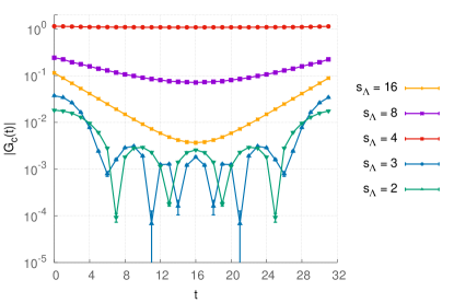
Figure 24: Time slice correlation functions on a $32\times 32$ lattice for fixed parameters $\kappa=0.26$ and $\lambda=0.02$. The orange curve shown in both graphs is the result obtained from a Langevin simulation with white noise for cutoff ${s_{\Lambda}}=16$. The full quantum theory is in the symmetric phase for the given choice of parameters. (Left) The plot shows the correlation function of time slices using a Pauli-Villars regularization function for different cutoffs. Halving the maximum lattice momentum cutoff to ${s_{\Lambda}}=8$ yields the violet curve showing that the mass decreases. It becomes minimal for ${s_{\Lambda}}=4$ were the theory is close to the critical point and the correlator is flat, see the red curve. Decreasing the cutoff further to ${s_{\Lambda}}=3$ and ${s_{\Lambda}}=2$ respectively shows that the correlator decays stronger again meaning that the mass in lattice units grows, but now with the theory being in the broken phase. (Right) The same setup as on the left is shown but here the sharp cutoff (7) is used. Note that for ${s_{\Lambda}}=2,3$ the correlator resembles a Bessel function which is an artifact of the noise correlation (84).

D.2 Alternative regularization functions

The regularization scheme used in Bern et al. (1987) is a Pauli-Villars regularization with cutoff parameter $\Lambda$. Explicitly, the regularization function is defined as

$$r_{\Lambda}(\Delta_{x})=\left(1-\frac{\Delta_{x}}{\Lambda^{2}}\right)^{-1}\,.$$ (96)

For most purposes it suffices to use the sharp regulator introduced in (7). However for certain cases, smooth regularization functions such as the Pauli-Villars type cutoff (96) or smooth approximations to the sharp cutoff may be required. A crucial disadvantage of the sharp cutoff is that it gives rise to artifacts appearing in the noise correlation function, as discussed for the continuum in Appendix C. Those are clearly visible in the correlation functions of time slices and pose difficulties, for instance to the determination of masses because standard exponential fit techniques are not applicable. The lattice version of the Pauli-Villars regularization function reads

$$r_{\tilde{s}_{\Lambda}}(\tilde{p}^{2}):=\left(1-\frac{\tilde{p}^{2}}{\tilde{s}^{2}_{\Lambda}}\right)^{-m}\,\delta_{x,y}\,,$$ (97)

where $m\in\mathbb{N}$ as introduced in Bern et al. (1987). Here $"\sim"$ refers to the physical momenta introduced in (60). Alternatively, a smooth approximation to the sharp regulator on the lattice reads

$$r_{\tilde{s}_{\Lambda}}(\tilde{p}^{2}):=\frac{1}{2}\left(1-\tanh\left[\alpha\left(\frac{\tilde{p}^{2}}{\tilde{s}^{2}_{\Lambda}}-1\right)\right]\right)\,,$$ (98)

where the parameter $\alpha\in\mathbb{R}_{+}$ can be tuned to vary the steepness around the cutoff momentum. Both of the regulator functions mentioned here are currently under study. They may reduce the above mentioned artifacts arising from the use of the sharp regulator. However, throughout the course of this work, we use the sharp regulator for all quantitative studies. Smooth regulators are only used in this section to illustrate a qualitatively different behaviour visible in the observables.

We discuss the effects of different choices of the regularization function by means of the two-point correlation function of time slices shown in Fig. 24. The correlators were computed for parameters $\kappa=0.26$, $\lambda=0.02$ on a $32\times 32$ lattice, that is for the same choice as for Fig. 6. Note, that the curves are represented in logarithmic scaling. The orange curve visible in both plots was computed in a simulation with Gaussian white noise (${s_{\Lambda}}=16$) and reproduces the hyperbolic cosine behaviour, typical for lattice correlators. The remaining correlators were produced in simulations with colored noise. The left plot in Fig. 24 stems from a simulation with a smooth Pauli-Villars regularization function. The external parameters $\kappa$ and $\lambda$ are chosen such that by cutting off ultraviolet modes we interpolate between the phases of the theory. Close to the phase transition the mass in lattice units approaches zero. This is consistent with the flattening of the correlation functions, see the violet (${s_{\Lambda}}=8$) and the red curve (${s_{\Lambda}}=4$). For ${s_{\Lambda}}=2,3$, see the green and blue curve, the theory is in the broken phase and the correlator bends for small Euclidean times loosing its typical exponential shape. This is a sign of an imprint of the regularization function in the correlator well visible for small ${s_{\Lambda}}$. This observation is also in agreement with the fact that the colored noise is correlated in Euclidean space-time. Moreover, consistently in the broken phase the mass grows again. For large Euclidean times the correlator also seems to retain the exponential behaviour. This might allow for the application of fits to extract mass values or the calculation of effective masses.

The right hand side of Fig. 24 shows the same setup as on the left but for the sharp regularization function (7). For intermediate ${s_{\Lambda}}=4,8$, see the red and violet curve, the results qualitatively agree with the corresponding results obtained with the Pauli-Villars regularization. For small ${s_{\Lambda}}=2,3$ however, see the green and blue curve, the correlator shapes differ. Although at small Euclidean times the correlator bends similarly, at larger times it oscillates. For illustrative reasons we show the modulus of the correlator $|G_{c}(t)|$. The sharp regularization function leaves an artifact imprinting a Bessel-like shape on the correlator, see also the discussion in Appendix C. The qualitative behaviour of the mass or correlation length agrees for both regularization functions used here. In Fig. 24 we do not show the classical correlation function since it is trivially zero. This is due to the gradient flow driving the field values into the classical minimum approaching a constant value as $\tau\to\infty$.

Appendix E Relation between stochastic regularization and the FRG

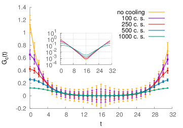
Figure 25: Equilibrium configurations from Langevin simulations with white noise are smoothed using the gradient flow. The correlation function of time slices $G_{c}(t)$ shows a similar behaviour as the colored noise result in Fig. 24.

Using the sharp momentum cutoff

$$r_{\Lambda}(p^{2})=\theta(\Lambda^{2}-p^{2})\,,$$ (99)

in the Fokker-Planck equation (6) allows for a simple relation of Stochastic Quantization with colored noise with functional renormalization group equations. To that end we write the probability distribution $P(\phi,\tau)$ in (6) for $\tau\to\infty$ as

$$P_{\Lambda}(\phi,\tau)=\exp\left(-S-\Delta S_{\Lambda}\right)\,,$$ (100)

where $\Delta S_{\Lambda}$ is defined in (9). Inserting (100) with (9) into (6) leads to the fixed point equation $\partial_{\tau}P_{\Lambda}=0$ in momentum space with

$$\left[\Bigl{(}1-r_{\Lambda}(p)\Bigr{)}\frac{\delta S}{\delta\phi_{p}}-r_{\Lambda}(p)\frac{\delta\Delta S_{\Lambda}}{\delta\phi_{p}}\right]P_{\Lambda}(\phi,\tau)=0\,.$$ (101)

With $(1-r_{\Lambda})r_{\Lambda}\equiv 0$ the two parts on the left hand side of (101) have to vanish separately. Now we use that

$$1-r_{\Lambda}(p)=\theta(p^{2}-\Lambda^{2})\,,$$ (102)

only applies to UV modes. Accordingly we have

$$\Bigl{(}1-r_{\Lambda}(p)\Bigr{)}\frac{\delta S}{\delta\phi_{p}}P_{\Lambda}(\phi,\tau)=0\,.$$ (103)

The prefactor in (103) does not vanish on the ultraviolet modes that do not satisfy the equations of motion, $\delta S/\delta\phi_{p}\neq 0$. For these modes (103) entails that the measure has to vanish,

$$\left.\vphantom{\frac{1}{1}}P_{\Lambda}(\phi_{p},\tau)\right|_{|p|>\Lambda}\stackrel{{\scriptstyle!}}{{=}}0\,,$$ (104)

hence the name sharp (UV) cutoff. (104) requires a diverging $\Delta S_{\Lambda}$ for the ultraviolet modes with $p^{2}>\Lambda^{2}$. In turn, the cutoff term is also constrained for $p^{2}<\Lambda^{2}$ by (101) with

$$r_{\Lambda}(p)\frac{\delta\Delta S_{\Lambda}}{\delta\phi_{p}}=0\,,$$ (105)

and $\Delta S_{\Lambda}$ has to vanish for the infrared modes. A simple choice for $\Delta S_{\Lambda}$ with these properties is given by

$$\Delta S_{\Lambda}[\phi]=\frac{1}{2}\int_{p}\phi_{p}\,\Lambda^{2}\left(\frac{1}{r_{\Lambda}(p)}-1\right)\phi_{-p}\,.$$ (106)

This cutoff term vanishes for momentum modes with $p^{2}<\Lambda^{2}$ and is infinite for $p^{2}>\Lambda^{2}$ leading to $P_{\Lambda}(\phi,\tau)=0$. This entails that the UV modes satisfy the classical equation of motions and no quantum effects are taken into account.

We close this section with the remark that smooth cutoff functions $r_{\Lambda}(p)$ for the noise do not lead to a measure of the type (100), as the related integrability relations are violated. This has been already observed in Bern et al. (1987) in a different context.

Appendix F A qualitative comparison of the gradient flow with colored noise

In this section, we briefly and qualitatively focus on the analogous behaviour of the gradient flow and the Langevin evolution with colored noise. Thereto, we consider a one-dimensional real scalar field theory and measure field configurations from a Langevin evolution with white noise. The configurations are stored and smoothed by means of the gradient flow. At each cooling step observables and corresponding errors are calculated. In Fig. 25 the two-point correlation function of time slices is depicted. The number of configurations is of $N_{\text{cf}}\approx O(10^{4})$ for $\kappa=0.47,\lambda=0.01$ and lattice size $N=32$. As configurations are smoothed by the gradient flow the errorbars shrink. To visualize this here, the errorbars are magnified by a factor $\sqrt{N_{\text{\tiny{cf}}}}$. In comparison with the result obtained using the sharp regulator in Fig. 24 we find the same behaviour of the correlator at small Euclidean times. As the configurations are cooled the correlator bends. This signalizes the effect of a heat diffusion equation which has been investigated in Bonati and D’Elia (2014) in the context of a massless scalar theory in $d$ dimensions. Note that the gradient flow for a scalar theory has exactly the form of a heat diffusion equation.

References

- Aarts (2016) G. Aarts, J. Phys. Conf. Ser. 706, 022004 (2016), arXiv:1512.05145 [hep-lat] .
- Aarts et al. (2016a) G. Aarts, F. Attanasio, B. Jäger, E. Seiler, D. Sexty, and I.-O. Stamatescu, AIP Conf. Proc. 1701, 020001 (2016a), arXiv:1412.0847 [hep-lat] .
- Aarts et al. (2013a) G. Aarts, F. A. James, J. M. Pawlowski, E. Seiler, D. Sexty, and I.-O. Stamatescu, JHEP 03, 073 (2013a), arXiv:1212.5231 [hep-lat] .
- Aarts et al. (2017) G. Aarts, E. Seiler, D. Sexty, and I.-O. Stamatescu, JHEP 05, 044 (2017), arXiv:1701.02322 [hep-lat] .
- Seiler et al. (2013) E. Seiler, D. Sexty, and I.-O. Stamatescu, Phys. Lett. B723, 213 (2013), arXiv:1211.3709 [hep-lat] .
- Sinclair and Kogut (2016) D. K. Sinclair and J. B. Kogut, PoS LATTICE2016, 026 (2016), arXiv:1611.02312 [hep-lat] .
- Nagata et al. (2016) K. Nagata, H. Matsufuru, J. Nishimura, and S. Shimasaki, PoS LATTICE2016, 067 (2016), arXiv:1611.08077 [hep-lat] .
- Langelage et al. (2014) J. Langelage, M. Neuman, and O. Philipsen, PoS LATTICE2013, 141 (2014), arXiv:1311.4409 [hep-lat] .
- Aarts et al. (2016b) G. Aarts, F. Attanasio, B. Jäger, and D. Sexty, JHEP 09, 087 (2016b), arXiv:1606.05561 [hep-lat] .
- Teper (1985) M. Teper, Phys. Lett. B162, 357 (1985).
- Garcia Perez et al. (1999) M. Garcia Perez, O. Philipsen, and I.-O. Stamatescu, Nucl. Phys. B551, 293 (1999), arXiv:hep-lat/9812006 [hep-lat] .
- Lüscher (2010) M. Lüscher, JHEP 08, 071 (2010), [Erratum: JHEP03,092(2014)], arXiv:1006.4518 [hep-lat] .
- Narayanan and Neuberger (2006) R. Narayanan and H. Neuberger, JHEP 03, 064 (2006), arXiv:hep-th/0601210 [hep-th] .
- Gonzalez-Arroyo and Okawa (2013) A. Gonzalez-Arroyo and M. Okawa, Phys. Lett. B718, 1524 (2013), arXiv:1206.0049 [hep-th] .
- Datta et al. (2016) S. Datta, S. Gupta, and A. Lytle, Phys. Rev. D94, 094502 (2016), arXiv:1512.04892 [hep-lat] .
- Capponi et al. (2016) F. Capponi, A. Rago, L. Del Debbio, S. Ehret, and R. Pellegrini, PoS LATTICE2015, 306 (2016), arXiv:1512.02851 [hep-lat] .
- Kagimura et al. (2015) A. Kagimura, A. Tomiya, and R. Yamamura, (2015), arXiv:1508.04986 [hep-lat] .
- Bornyakov et al. (2015) V. G. Bornyakov et al., (2015), arXiv:1508.05916 [hep-lat] .
- Bonati and D’Elia (2014) C. Bonati and M. D’Elia, Phys. Rev. D89, 105005 (2014), arXiv:1401.2441 [hep-lat] .
- Bern et al. (1985) Z. Bern, M. B. Halpern, L. Sadun, and C. H. Taubes, Phys. Lett. B165, 151 (1985).
- Bern et al. (1987) Z. Bern, M. B. Halpern, L. Sadun, and C. H. Taubes, Nucl. Phys. B284, 1 (1987), and further publications by this group.
- Kadanoff (1966) L. P. Kadanoff, Physics 2, 263 (1966).
- Berges et al. (2002) J. Berges, N. Tetradis, and C. Wetterich, Phys. Rept. 363, 223 (2002), arXiv:hep-ph/0005122 .
- Polonyi (2003) J. Polonyi, Central Eur.J.Phys. 1, 1 (2003), arXiv:hep-th/0110026 [hep-th] .
- Pawlowski (2007) J. M. Pawlowski, Annals Phys. 322, 2831 (2007), arXiv:hep-th/0512261 [hep-th] .
- Delamotte (2012) B. Delamotte, Lect. Notes Phys. 852, 49 (2012), arXiv:cond-mat/0702365 [cond-mat.stat-mech] .
- Rosten (2012) O. J. Rosten, Phys. Rept. 511, 177 (2012), arXiv:1003.1366 [hep-th] .
- Metzner et al. (2012) W. Metzner, M. Salmhofer, C. Honerkamp, V. Meden, and K. Schönhammer, Reviews of Modern Physics 84, 299 (2012), arXiv:1105.5289 [cond-mat.str-el] .
- Parisi and Wu (1981) G. Parisi and Y. Wu, Sci.Sin. 24, 483 (1981).
- Damgaard and Huffel (1987) P. H. Damgaard and H. Huffel, Phys.Rept. 152, 227 (1987).
- Aarts et al. (2013b) G. Aarts, L. Bongiovanni, E. Seiler, D. Sexty, and I.-O. Stamatescu, Eur. Phys. J. A49, 89 (2013b), arXiv:1303.6425 [hep-lat] .
- Batrouni et al. (1985) G. G. Batrouni, G. R. Katz, A. S. Kronfeld, G. P. Lepage, B. Svetitsky, and K. G. Wilson, Phys. Rev. D 32, 2736 (1985).
- Binder (1981) K. Binder, Zeitschrift für Physik B Condensed Matter 43, 119–140 (1981).
- De et al. (2005) A. K. De, A. Harindranath, J. Maiti, and T. Sinha, Phys. Rev. D72, 094503 (2005), arXiv:hep-lat/0506002 [hep-lat] .
- Wegner and Houghton (1973) F. J. Wegner and A. Houghton, Phys. Rev. A8, 401 (1973).
- Montvay and Münster (1997) I. Montvay and G. Münster, Quantum fields on a lattice, Cambridge Monographs on Mathematical Physics (Cambridge University Press, 1997).