Supporting Material:
Fast data sorting with modified principal component analysis to distinguish unique single molecular break junction trajectories

I Principal components as description of variance

The relationships between the eigenvalues, eigenvectors, and variance in a correlation matrix were demonstrated by PearsonPearson (1901). Here we wish to summarize the relevant mathematics and notation used in the main text.

Given an $m\times n$ data matrix, $\mathbf{X}$, with $m$ variables and $n$ measurements, we wish to find a transformation, $\mathbf{a}_{k}$, such that

$$\mathbf{p}_{k}=\mathbf{a}_{k}^{T}\mathbf{X},~{}k=1,\ldots,m.$$ (S1)

Specifically, we wish to choose $\mathbf{a}_{k}$ such that

$$var\left[\mathbf{p}_{k}\right]=\langle\mathbf{p}^{2}_{k}\rangle-\langle\mathbf{p}_{k}\rangle^{2}$$ (S2)

is maximized, and

$$cov\left[\mathbf{p}_{k},\mathbf{p}_{l}\right]=0,~{}k,l=1,\ldots,m,~{}k>l\geq 1.$$ (S3)

To determine the form of $\mathbf{a}_{k}$, Eq. S2 can be expanded

$$var\left[\mathbf{p}_{k}\right] =\langle\mathbf{p}^{2}_{k}\rangle-\langle\mathbf{p}_{k}\rangle^{2}$$

$$=\sum_{i,j=1}^{n}a_{ik}a_{jk}\langle x_{i}x_{j}\rangle-\sum_{i,j=1}^{n}a_{ik}a_{jk}\langle x_{i}\rangle\langle x_{j}\rangle$$

$$=\sum_{i,j=1}^{n}a_{ik}a_{jk}S_{ij},~{}S_{ij}\equiv\sigma_{x_{i}x_{j}}=\langle x_{i}x_{j}\rangle-\langle x_{i}\rangle\langle x_{j}\rangle$$

$$=\mathbf{a}_{k}^{T}\mathbf{S}\mathbf{a}.$$

$\mathbf{S}$ is the covariance matrix for the data matrix $\mathbf{X}$. To find $\mathbf{a}_{k}$ which maximizes $var[\mathbf{p}_{k}]$, subject to $\mathbf{a}_{k}^{T}\mathbf{a}_{k}=1$, we will use the method of Lagrangian multipliers. This amounts to maximizing

$$\mathbf{a}_{k}^{T}\mathbf{S}\mathbf{a}_{k}-\lambda(\mathbf{a}_{k}^{T}\mathbf{a}_{k}-1)$$

by differentiating and finding the zeros

$$\mathbf{S}\mathbf{a}_{k}-\lambda\mathbf{a}_{k} =0$$

$$(\mathbf{S}-\lambda\mathbf{I}_{m})\mathbf{a}_{k} =0.$$

Evidently $\mathbf{a}_{k}$ is an eigenvector of the covariance matrix, $\mathbf{S}$, and $\lambda_{k}$ is the corresponding eigenvalue. Therefore we also know

$$var\left[\mathbf{p}_{1}\right] =\mathbf{a}_{1}^{T}\mathbf{S}\mathbf{a}_{1}$$

$$=\mathbf{a}_{1}^{T}\lambda_{1}\mathbf{a}_{1}$$

$$=\lambda_{1}.$$

Therefore $\lambda_{1}$ is the largest eigenvalue and $\mathbf{a}_{1}$, the first principal component (PC), projects the data matrix $\mathbf{X}$ along the direction which maximizes the variance. Furthermore, $\lambda_{2}$ is the second largest eigenvalue (Eq. S3) and $\mathbf{a}_{2}$, the second PC, projects the data matrix $\mathbf{X}$ in a direction, orthogonal to $\mathbf{a}_{1}$, which achieves the second largest variance. Specifically, $sign\left[p_{1i}\right]$ describes whether measurement $i$ more closely resembles $\mathbf{a}_{1}$ or $-\mathbf{a}_{1}$. This will be used as the sorting criteria to separate the following data sets into groups.

Finally, all of the eigenvectors together account for the entirety of the variance within the data set, and

$$V_{k}=\frac{\lambda_{k}}{\sum_{k=1}^{m}\lambda_{k}}\cdot 100\%$$

meaning each eigenvalue describes the amount, given as a percentage of the total, of variance explained, $V_{k}$. If the data matrix comprised entirely of randomly distributed data, then the covariance matrix would be unity along the diagonal, and zero elsewhere. In other words, no other variables would be correlated at all, except with themselves. In this case, the eigenvalues, and variance explained, would be degenerate, with value of unity. This is the one extreme, when the data is random. The other extreme is when the data is all perfectly correlated. In this case, one PC would be sufficient to describe 100% of the variance. Thus, the degree to which the variance explained falls off is a good description of the amount of randomness is in the data set. If the variance explained versus PC number is nearly flat, it will indicate there is a lot of randomness in the data, and if it is steep it will indicate that there is a strong trend in the data.

Normally it is necessary to normalize each variable and offset the mean to zero, thus giving each variable equal scaling, before calculating $\mathbf{S}$. However, for our purposes it is more desirable to calculate the correlation matrix, $C$, introduced by Halbritter, et al.Halbritter et al. (2010); Makk et al. (2012) than the covariance matrix, $\mathbf{S}$

$$C_{i,j}=\frac{\langle\left[x_{i}-\langle x_{i}\rangle\right]*\left[x_{j}-\langle x_{j}\rangle\right]\rangle}{\sqrt{\langle\left[x_{i}-\langle x_{i}\rangle\right]^{2}\rangle\langle\left[x_{j}-\langle x_{j}\rangle\right]^{2}\rangle}}.$$ (S4)

because the denominator ensures each variable has been offset and normalized. In general, covariance between different variables in a data matrix can be misleading, because the different variables may have different units at vastly different scales. The denominator in Eq. S4 removes this vagueness by removing the units and normalizing all variables to vary in the range from $[-1,1]$. It is therefore useful to use Eq. S4 for two reasons: 1. analysis using the correlation matrix has become a standard analysis method in break junction research, and 2. the normalized nature of the correlation matrix allows it to be immediately utilized in principal componant analysis methods.

II Mechanically controlled break junctions

A mechanically controlled break junction (MCBJ) was used to create single molecular break junctions. MCBJ utilizes a piezo stack to rapidly open and close a $0.1~{}\textrm{mm}$ diameter Au wire (Goodfellow, 99.99%) inside a liquid cell filled with the molecular solution. Each trace [example traces in Fig. 1(c)] started at high conductance with a closed Au-Au circuit. After the last Au-Au atomic contact broke, the conductance dropped rapidly from $10^{0}~{}\textrm{G}_{0}$. An ideal junction which was mechanically stable and free of contamination had a period of snap-back just following the breaking of the Au-Au bond in which the conductance dropped so quickly that the trace showed no significant change in displacement while the conductance dropped by two or three orders of magnitude.Huang et al. (2015) If a molecule was trapped in the junction, a plateau was seen in the trace while the conductance across the molecule was measured. Finally, the Au-molecule-Au junction broke and the conductance dropped to the open circuit sensitivity of the amplifier, at approximately $10^{-9}~{}\textrm{G}_{0}$. The separation of the Au leads, $\Delta z$, was deduced from the length of the molecular plateau feature, from after the Au-Au junction to before the open circuit.

A very permissive pre-analysis selection criteria was applied to remove traces which did not meet the following criteria:

1. start above a conductance of at least $10^{0.5}~{}\textrm{G}_{0}$ - this ensured that each junction began with a Au-Au contact

2. end below the open circuit sensitivity of the amplifier, at $10^{-9}~{}\textrm{G}_{0}$ - this ensured that each trace opened completely

3. the trace had to be shorter than a maximum length of $6~{}\textrm{nm}$ - traces longer than this do not involve the molecule of study ($1.6~{}\textrm{nm}$ long), but may be due to contamination or environmental disturbances.

This criteria removed between $2$ and $20\%$ of the traces in a data set, depending on how stable the experiment was.

III Synthetic procedures

All commercial chemicals were used without further purification. Anhydrous solvents were dried through an HPLC column on an Innovative Technology Inc. solvent purification system. Column chromatography was carried out using 40-60 $\mu$m mesh silica (Fluorochem). NMR spectra were recorded on: Bruker Avance-400, Varian VNMRS-600, VNMRS-700 and Varian Inova 500 spectrometers. Chemical shifts are reported in ppm relative to tetramethylsilane (0.00 ppm). Melting points were determined in open-ended capillaries using a Stuart Scientific SMP40 melting point apparatus at a ramping rate of 2 $\mathrm{\SIUnitSymbolCelsius}$/min. Mass spectra were measured on a Waters Xevo OTofMS with an ASAP probe. Electron ionization (EI) mass spectra were recorded on a Thermoquest Trace or a Thermo-Finnigan DSQ.

Figure S1: Synthesis of $\mathbf{M}_{\pi}$. Reagents and conditions: Pd(PPh3)4, CuI, THF/Et3N, 18 h, 60 $\mathrm{\SIUnitSymbolCelsius}$, 64%.

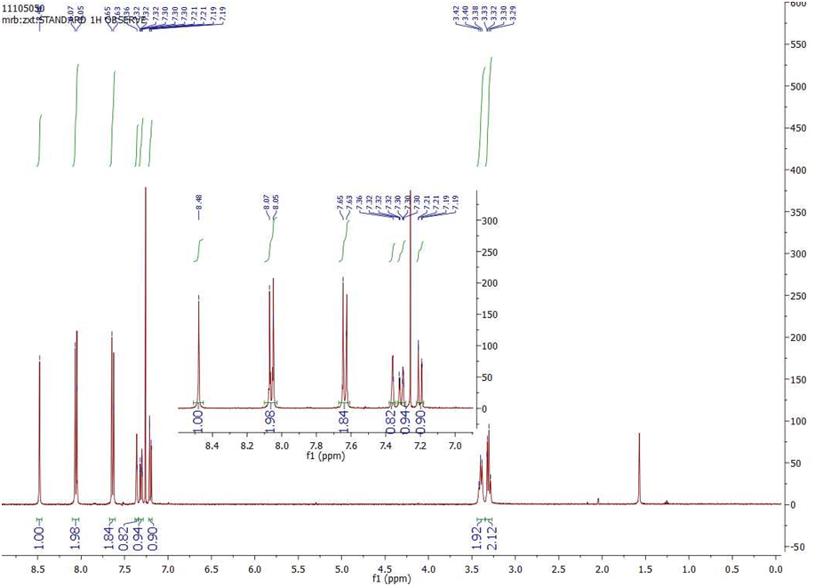
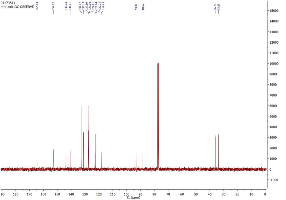
To a solution of 1Moreno-García et al. (2013) (Fig. S1, 100 mg, 0.63 mmol), Pd(PPh3)4 (36 mg, 0.03 mmol) and CuI (6 mg, 0.03 mmol) in THF/Et3N (3:1 v/v) (25 ml), was added 2Salvanna et al. (2013) (Fig. S1, 142 mg, 0.63 mmol) and the reaction was stirred at 60 $\mathrm{\SIUnitSymbolCelsius}$ for 18 h under argon (which had been dried by passage through a column of phosphorus pentoxide) before the solvent was removed by vacuum evaporation and the residue was purified by column chromatography in DCM which gave $\mathbf{M}_{\pi}$ as a yellow solid (122 mg, 64% yield). m.p.: decomp. over 250 $\mathrm{\SIUnitSymbolCelsius}$. HR-MS (ASAP+) m/z Calcd for C18H13N2OS [M+H]⁺ 305.0749, found m/z : [M+H]⁺ 305.0753. Anal. Calc. for C18H12N2O: C, 71.03; H, 3.97; N, 9.20. Found: C, 71.13; H, 3.92; N, 9.11. ^1H NMR (Fig. S3, 400 MHz, CDCl3) $\delta$ 8.48 (s, 1H), 8.06 (d, J = 8.8, 2H), 7.64 (d, J = 8.8, 2H), 7.36 (m, 1H), 7.31 (m, 1H), 7.20 (m, 1H), 3.40 (t, J = 7.8 Hz, 2H), 3.30 (t, J = 7.8 Hz, 2H). ^13C NMR (Fig. S4, 101 MHz, CDCl3) $\delta$ 164.61, 152.88, 143.73, 140.71, 132.27, 131.19, 127.60, 127.54, 127.21, 122.74, 122.25, 118.30, 93.12, 88.22, 36.04, 33.69.

Figure S2: Synthesis of $\mathbf{M}_{\sigma}$. Reagents and conditions: Pd/C, THF, 24 h, r.t., 65%.

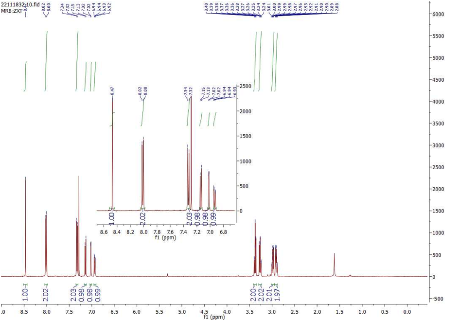
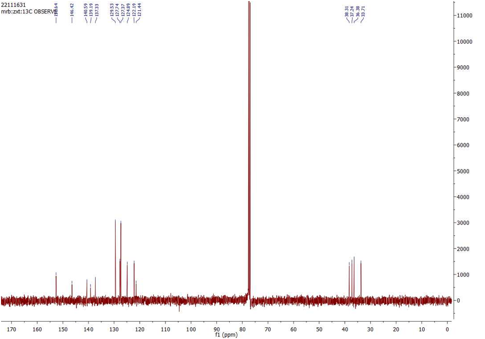
A mixture of $\mathbf{M}_{\pi}$ (25 mg, 0.08 mg) and Pd/C (10 mg, 10wt. %) in THF under H2 was stirred at r.t. for 24 h before the mixture was filtered through a silica pad. A yellow product $\mathbf{M}_{\sigma}$ (Fig. S2, 16 mg, 65%) was obtained from recrystallisation in DCM/EtOH. m.p.: decomp. over 265 $\mathrm{\SIUnitSymbolCelsius}$. HR-MS (ASAP+) m/z Calcd for C18H17N2OS [M+H]⁺ 309.1062, found m/z : [M+H]⁺ 309.1073. Anal. Calc. for C18H16N2OS: C, 70.10; H, 5.23; N, 9.08. Found: C, 70.24; H,5.30; N, 9.20. ^1H NMR (Fig. S5, 400 MHz, CDCl3) $\delta$ 8.47 (s, 1H), 8.01 (d, J = 8.3 Hz, 2H), 7.33 (d, J = 8.3 Hz, 2H), 7.14 (d, J = 7.8 Hz, 1H), 7.02 (s, 1H), 6.93 (d, J = 7.8, 1H), 3.38 (t, J = 7.6, 1.3 Hz, 2H), 3.26 (t, J = 7.6, 1.3 Hz, 2H), 2.99 (m, 2H), 2.90 (m, 2H). ^13C NMR (Fig. S6, 101 MHz, CDCl3) $\delta$ 152.64, 146.42, 140.59, 139.19, 137.33, 129.53, 127.74, 127.37, 124.89, 122.19, 121.44, 38.31, 37.24, 36.38, 33.71.

Figure S3: H^1 NMR Spectrum for $\mathbf{M}_{\pi}$.

Figure S4: C^13 NMR Spectrum for $\mathbf{M}_{\pi}$.

Figure S5: H^1 NMR Spectrum for $\mathbf{M}_{\sigma}$.

Figure S6: C^13 NMR Spectrum for $\mathbf{M}_{\sigma}$.

IV Molecule solutions preparation

Two stock solutions of $0.1~{}\textrm{M}$ molecule in 1:4 THF:TMB (v/v) were prepared. $0.1~{}\textrm{mM}$ solutions of $\mathbf{M}_{\sigma}$ and $\mathbf{M}_{\pi}$ were prepared from these. Three mixtures were also prepared from the stock solutions:

1. Mix 1 (1:3 #/#): $0.025~{}\textrm{mM}$ $\mathbf{M}_{\sigma}$ and $0.075~{}\textrm{mM}$ $\mathbf{M}_{\pi}$

2. Mix 2 (1:1 #/#): $0.050~{}\textrm{mM}$ $\mathbf{M}_{\sigma}$ and $0.050~{}\textrm{mM}$ $\mathbf{M}_{\pi}$

3. Mix 3 (3:1 #/#): $0.075~{}\textrm{mM}$ $\mathbf{M}_{\sigma}$ and $0.025~{}\textrm{mM}$ $\mathbf{M}_{\pi}$.

V Experimental results

V.1 PC sorting on $\mathbf{X}_{1}$ using $PC_{2}$

Although any PC (or combination of PCs) from the diagonalized correlation matrix [shown as an intensity plot in Fig. 2(b)] may be used to sort the data matrix ([Fig. 2(a)], to yield meaningful groups, the aim of this Letter was to demonstrate how PC sorting sorted $\mathbf{X}_{1}$ into groups based on which molecule, $\mathbf{M}_{\pi}$ or $\mathbf{M}_{\sigma}$, was measured in the junction, and $PC_{1}$ successfully did this.

For completeness, the results when $\mathbf{X}_{1}$ was sorted using $PC_{2}$ was shown here in Fig. S8. Figure S7(a) is a reproduction of Fig. 2(b) from the main text and Fig. S7(b) is the eigenvalues, converted to variance explained, resulting from the diagonalization of the correlation matrix. Figures S8(a,b) were identical to Figs. 3(a,b), but projecting $\mathbf{X}_{1}$ onto $PC_{2}$ instead of $PC_{1}$ yielded new results in Figs. S8(c-e). Specifically, it was evident in Fig. S8(d) that $PC_{2}$ had not sorted $\mathbf{X}_{1}$ into groups containing only $\mathbf{M}_{\pi}$ or $\mathbf{M}_{\sigma}$ junctions because both $\mathbf{X}_{1+}$ and $\mathbf{X}_{1-}$ did not have single mode distributions in their total 1DHs [Fig. S8(d)]. $PC_{2}$ was largest in the bins corresponding to conductances of approximately $10^{-1}$ to $10^{-3}~{}\textrm{G}_{0}$, higher than either molecule. Figure S7(a) contains a region of weak anticorrelation at approximately $(10^{-2}~{}\textrm{G}_{0},10^{-4}~{}\textrm{G}_{0})$ which $PC_{2}$ may be describing. Instead of separating junctions based on criteria relating to the presence or absence of a molecule, or the presence of $\mathbf{M}_{\pi}$ or $\mathbf{M}_{\sigma}$, it was likely that sorting with $PC_{2}$ separated $\mathbf{X}_{1}$ into junctions which have a nearly ideal snap-back region, where the conductance trace drops quickly in the range $10^{-1}$ to $10^{-3}~{}\textrm{G}_{0}$ with no appreciable change in displacement, and junctions which exhibit some significant displacement in this same region. The difference in these two types of junctions can be seen in the 1D histograms with the presence or absence of counts in the bins corresponding to this conductance range. This presence or absence of counts was likely the variance in the data set which resulted in the large values in $PC_{2}$ in this conductance range. The likely causes of the non-ideal behavior in the snap-back region of the conductance traces were contamination or loss of mechanical stability.

Figure S7: (a) Intensity plot of correlation matrix from $\mathbf{X}_{1}$, and (b) eigenvalues from correlation matrix as variance explained in a semilog plot.

Figure S8: PCA analysis on Mix 1 using $PC_{2}$. (a) $PC_{1}$ (blue) and $PC_{2}$ (orange) plotted vs. bin number; (b) $PC_{1}$ vs. $PC_{2}$ from bin 1 (red) to bin 128 (blue); (c) histogram constructed from single 1D histograms projected onto $PC_{2}$ - curves in the red (green) bins had negative (positive) projections; (d) negatively (7129 curves) and positively (4541 curves) projected curves were sorted into separate groups and total 1D histograms were constructed - gray histogram is total 1D histogram from entire data set (80% of 14543 curves); (e) plateau lengths were determined for each trace in the negative (red) and positive (green) groups and the entire data set (gray) and histograms were constructed for each.

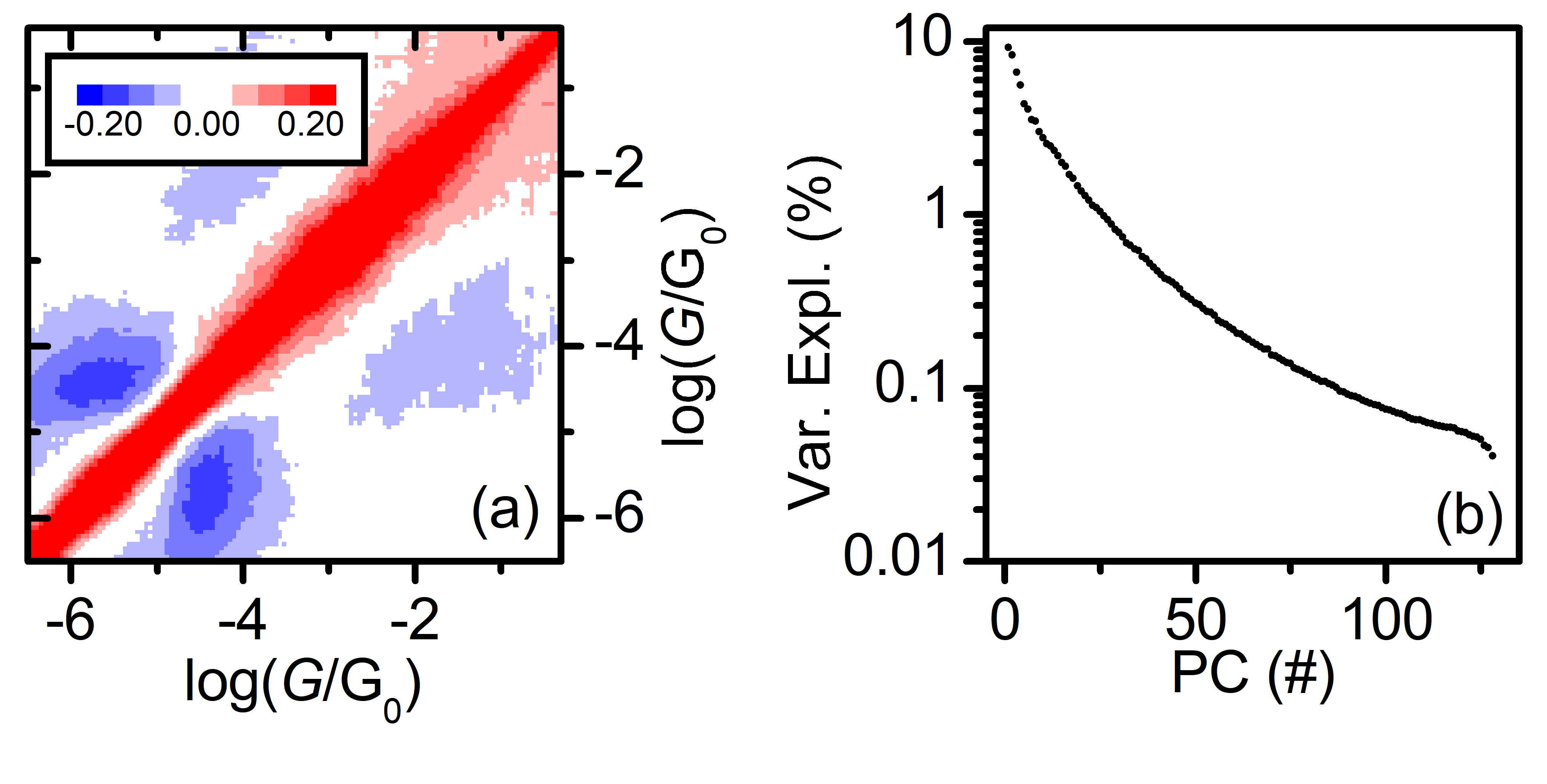
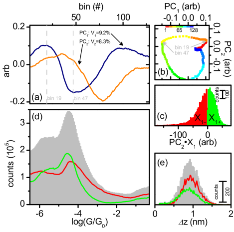
Figure S9(a) shows all eight of the first PCs from $\mathbf{X}_{1}$. The first 2 PCs (these were the two we used for analysis above and in the main text) had a qualitatively different nature than the remaining PCs. There appeared to be an emerging pattern as we looked at PCs $3-8$. At first glance PCs 3-8 had a sinusoidal structure, with each further PC having one more node than the previous. We did not wish to speculate on the nature of this pattern, except to suggest that whatever the cause, it was not highly descriptive of the molecular features.

Figure S9: (a) left axis is the total 1D histogram (in grey) from $\mathbf{X}_{1}$ ; right axis is first 8 PCs from $\mathbf{X}_{1}$, and (b) eigenvalues plotted as variance explained in a linear plot.

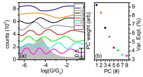
Figure S9(b) plotted the first 8 eigenvalues, plotted as variance explained, on a linear scale. The semilog plot in Fig. S7(b) already emphasized the extreme fall off of variance explained as we look at further PCs, and Fig. S9(b) supported this claim.

To reiterate, many different PCs may be considered when applying this sorting method. However, we note that the rapid fall off of variance explained, as shown in Figs. S7(b) and S9(b), suggests that this specific experiment contains much of the salient variance in the first few PCs. We also note that the emergence of a regular pattern in PCs $3-8$, shown in Fig. S9(a), indicates that those PCs are governed by variances not involving the molecules. Finally, we emphasize our stated goal: to find a simple and fast approach to meaningfully separate two groups from a single data set. If we find a PC which does this in the first or second PC, then that PC will explain larger variance than any subsequent PC we may find.

V.2 PC sorting on two further mixtures of $\mathbf{M}_{\pi}$ and $\mathbf{M}_{\sigma}$: Mix 2 and Mix 3

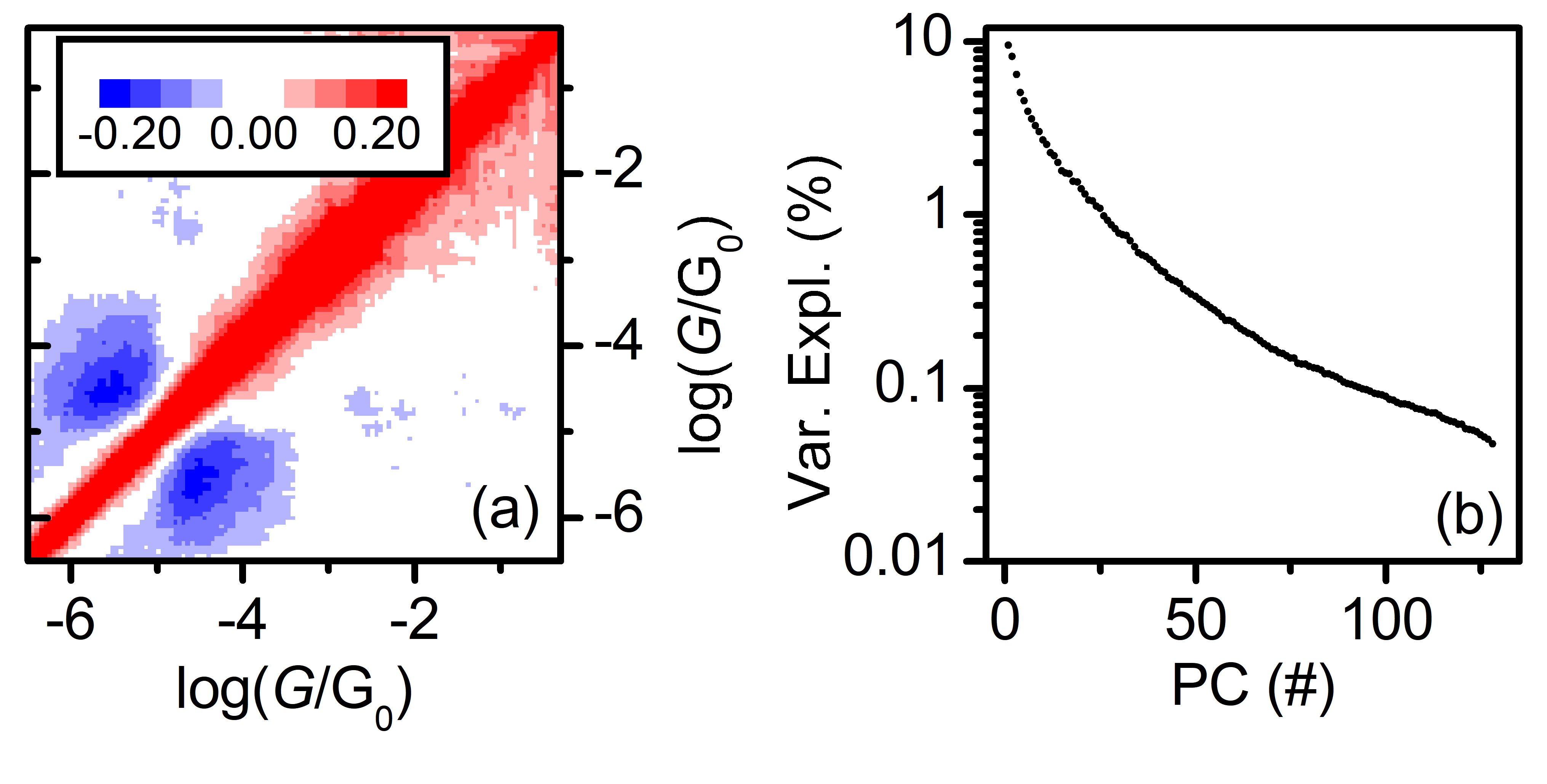
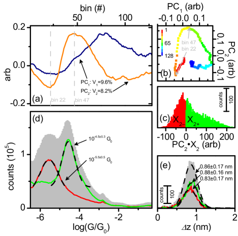
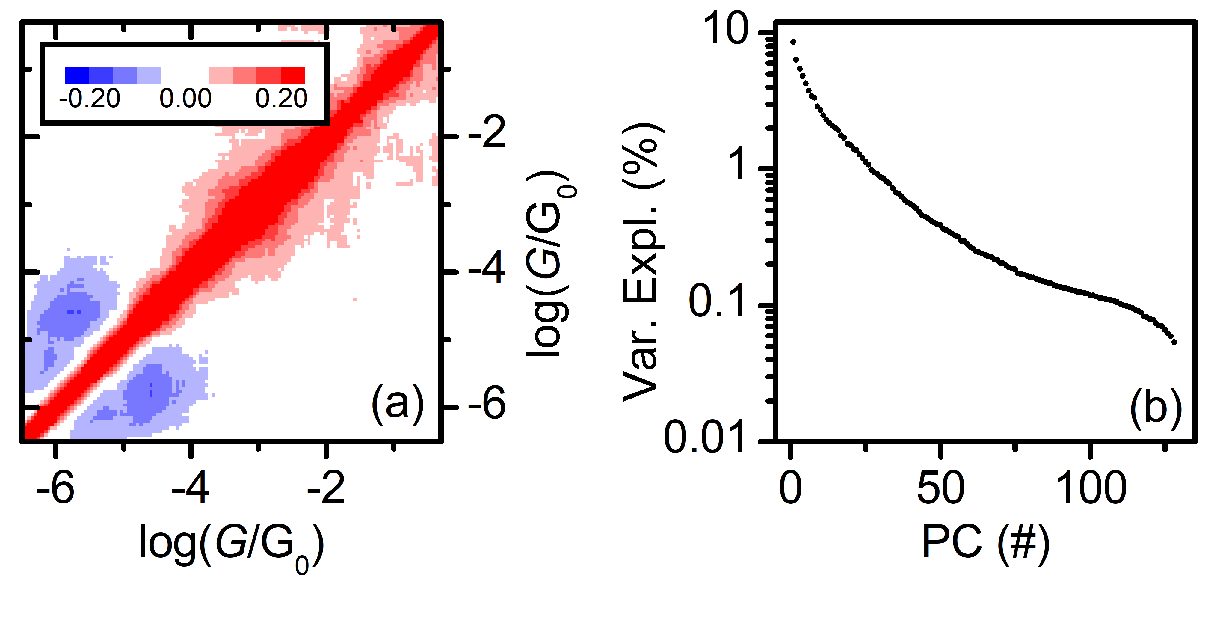
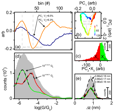
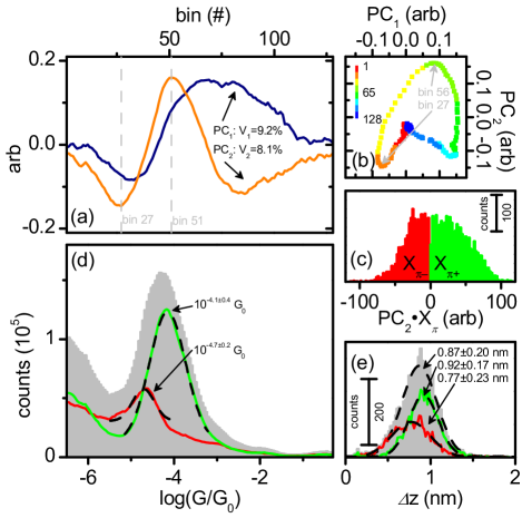
To demonstrate further the effectiveness of PC sorting we measured two more systems. Besides the 1:3 $\mathbf{M_{\sigma}}$:$\mathbf{M_{\pi}}$ mixture, Mix 1, described in the main text, and above, two further mixtures, Mix 2 and Mix 3 were prepared and measured with MCBJ. Correlation matrices, plotted as intensity plots, can be seen in Figs. S10 and S12(a)and the eigenvalues, converted to variance explained, can be seen in Figs. S10 and S12(b). For both Mix 2 and Mix 3, $PC_{2}$ was most successful at sorting the junctions into groups of $\mathbf{M}_{\pi}$ and $\mathbf{M}_{\sigma}$ junctions. In both cases, $PC_{2}$ [Figs. S11,S13(a)] had maxima and minima in the same bins corresponding to molecular conductances of $\mathbf{M}_{\pi}$ and $\mathbf{M}_{\sigma}$, and thus was the logical choice. Plots of $PC_{1}$ vs $PC_{2}$ [Figs. S11 and S13(b)] clarified this.

Using PC sorting, $\mathbf{X}_{2}$ was sorted [Fig. S11(c)] into 2505 curves in $\mathbf{X}_{2-}$ and 3196 curves in $\mathbf{X}_{2+}$. $\mathbf{X}_{2-}$ and $\mathbf{X}_{2+}$ were associated with junctions involving $\mathbf{M}_{\sigma}$ and $\mathbf{M}_{\pi}$, respectively, by comparing the 1DHs [Fig. S11(d)] with $\mathbf{M}_{\sigma}$ and $\mathbf{M}_{\pi}$ measured separately. The average plateaus were the same length [Fig. S11(e)].

Figure S10: (a) Intensity plot of correlation matrix from $\mathbf{X}_{2}$, and (b) eigenvalues from correlation matrix as variance explained in a semi-log plot.

Figure S11: PC sorting on Mix 2 using $PC_{2}$. (a) $PC_{1}$ (blue) and $PC_{2}$ (orange) plotted vs. bin number; (b) $PC_{1}$ vs. $PC_{2}$ from bin 1 (red) to bin 128 (blue); (c) histogram constructed from single 1D histograms projected onto $PC_{2}$ - curves in the red (green) bins had negative (positive) projections; (d) negatively (7129 curves) and positively (4541 curves) projected curves were sorted into separate groups and total 1D histograms were constructed - gray histogram is total 1D histogram from entire data set (80% of 14543 curves); (e) plateau lengths were determined for each trace in the negative (red) and positive (green) groups and the entire data set (gray) and histograms were constructed for each.

PC sorting of $\mathbf{X}_{3}$ garnered strikingly similar results, except the numbers of junctions involving $\mathbf{M}_{\sigma}$ and $\mathbf{M}_{\pi}$ changed (5265 $\mathbf{M}_{\pi}$ and 4823 $\mathbf{M}_{\sigma}$). Also, in the case of $\mathbf{X}_{3}$, $\mathbf{X}_{3-}$ was associated with junctions involving $\mathbf{M}_{\pi}$, while $\mathbf{X}_{3+}$ was associated with $\mathbf{M}_{\sigma}$.

Figure S12: (a) Intensity plot of correlation matrix from $\mathbf{X}_{3}$, and (b) eigenvalues from correlation matrix as variance explained in a semi-log plot.

Figure S13: PC sorting on Mix 3 using $PC_{2}$. (a) $PC_{1}$ (blue) and $PC_{2}$ (orange) plotted vs. bin number; (b) $PC_{1}$ vs. $PC_{2}$ from bin 1 (red) to bin 128 (blue); (c) histogram constructed from single 1D histograms projected onto $PC_{2}$ - curves in the red (green) bins had negative (positive) projections; (d) negatively (7129 curves) and positively (4541 curves) projected curves were sorted into separate groups and total 1D histograms were constructed - gray histogram is total 1D histogram from entire data set (80% of 14543 curves); (e) plateau lengths were determined for each trace in the negative (red) and positive (green) groups and the entire data set (gray) and histograms were constructed for each.

V.3 PC sorting on $\mathbf{X}_{\pi}$ using $PC_{2}$

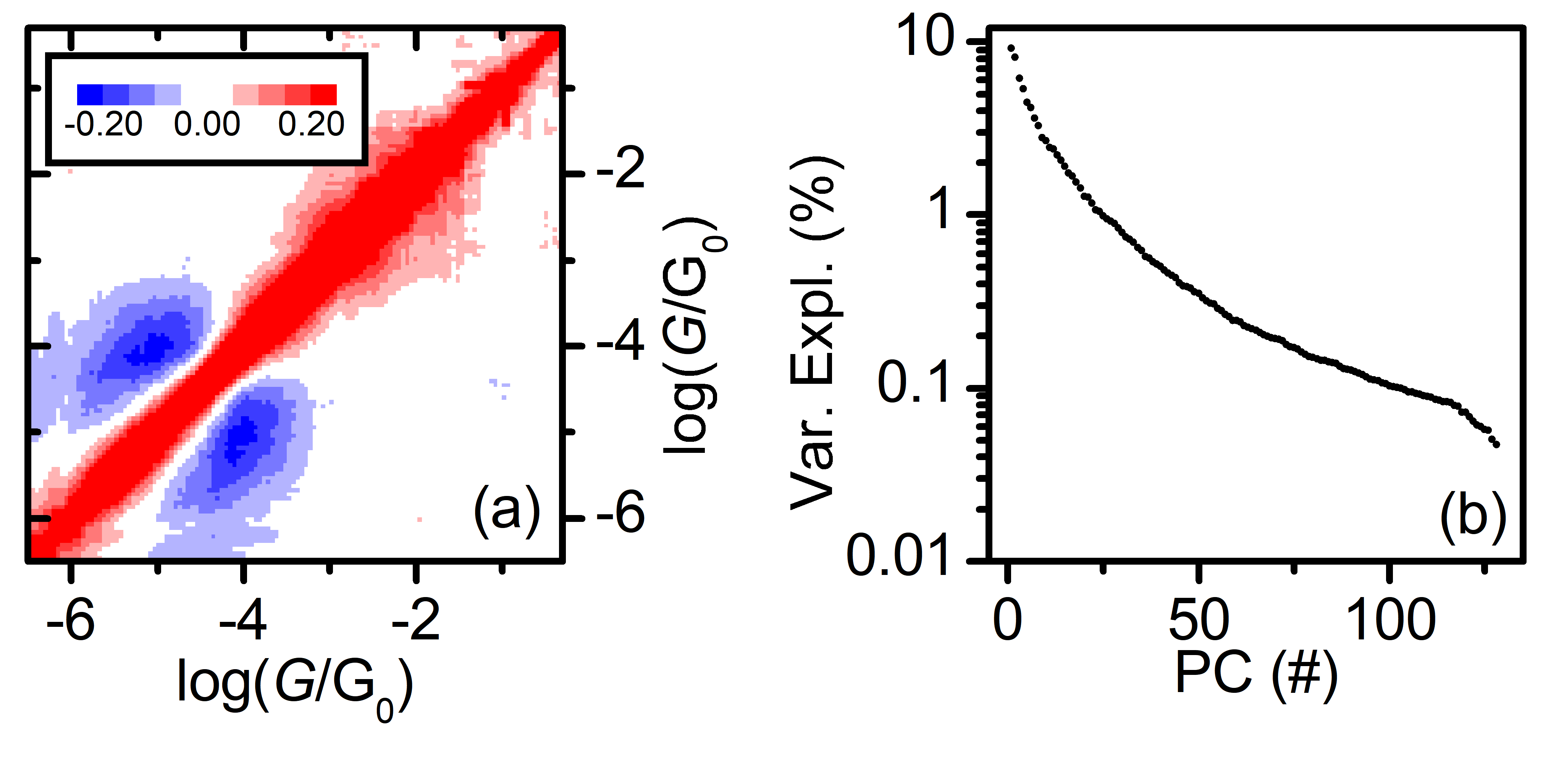
The PC sorting steps which yielded Fig. 4 are shown here. Diagonalizing the correlation matrix [intensity plot in Fig. S14(a)] yielded eigenvalues, converted to variance explained, plotted in Fig. S14(b). $PC_{1}$ and $PC_{2}$ [Figs. S15(a,b)] were very similar in the bins involving the molecular conductance of $\mathbf{M}_{\pi}$, but $PC_{2}$ was slightly more dominant in the pertinent conductance range, so it was used to sort $\mathbf{X}_{\pi}$ into $\mathbf{X}_{\pi-}$ and $\mathbf{X}_{\pi+}$ [Fig. S15(c)].

Figure S14: (a) Intensity plot of correlation matrix from $\mathbf{X}_{\pi}$, and (b) eigenvalues from correlation matrix as variance explained in a semi-log plot.

Figure S15: PC sorting on $\mathbf{X}_{\pi}$ using $PC_{2}$. (a) $PC_{1}$ (blue) and $PC_{2}$ (orange) plotted vs. bin number; (b) $PC_{1}$ vs. $PC_{2}$ from bin 1 (red) to bin 128 (blue); (c) histogram constructed from single 1D histograms projected onto $PC_{2}$ - curves in the red (green) bins had negative (positive) projections; (d) negatively (7129 curves) and positively (4541 curves) projected curves were sorted into separate groups and total 1D histograms were constructed - gray histogram is total 1D histogram from entire data set (80% of 14543 curves); (e) plateau lengths were determined for each trace in the negative (red) and positive (green) groups and the entire data set (gray) and histograms were constructed for each.

V.4 Master curve fitting

The vertical bins in the 2D histogram (displacement) can each be fit to a Gaussian following procedures previously published Moreno-García et al. (2013). The mean of each fit can be assembled into an array, called the master curve, which describes the average trace in the data set. 2D histograms for $\mathbf{X}_{\pi-}$ and $\mathbf{X}_{\pi+}$ were fit to determine master curves [Figs. S16(a,b)]. The molecular plateau region was then linearly fit to determine the slope of the plateau. In the case of $\mathbf{X}_{\pi-}$, two regions were fit to two separate slopes. The slopes were converted from $log_{10}$ to $log_{e}$ for purposes of referring to Eq. 1 (in the main text) and Ref. Huang et al. (2015).

Figure S16: Master curves fit to 2D histograms from (a) $\mathbf{X}_{\pi-}$ and (b) $\mathbf{X}_{\pi+}$. Grey lines are linear fits to molecular plateaus. Master curve in (a) was fit to two lines with two separate slopes.

References

- Pearson (1901) K. Pearson, The London, Edinburgh, and Dublin Philosophical Magazine and Journal of Science 2, 559 (1901).
- Halbritter et al. (2010) A. Halbritter, P. Makk, S. Mackowiak, S. Csonka, M. Wawrzyniak, and J. Martinek, Phys. Rev. Lett. 105, 266805 (2010).
- Makk et al. (2012) P. Makk, D. Tomaszewski, J. Martinek, Z. Balogh, S. Csonka, M. Wawrzyniak, M. Frei, L. Venkataraman, and A. Halbritter, ACS Nano 6, 3411 (2012).
- Huang et al. (2015) C. Huang, A. V. Rudnev, W. Hong, and T. Wandlowski, Chem. Soc. Rev. 44, 889 (2015).
- Moreno-García et al. (2013) P. Moreno-García, M. Gulcur, D. Z. Manrique, T. Pope, W. Hong, V. Kaliginedi, C. Huang, A. S. Batsanov, M. R. Bryce, C. Lambert, and T. Wandlowski, J. Am. Chem. Soc. 135, 12228 (2013).
- Salvanna et al. (2013) N. Salvanna, G. C. Reddy, B. R. Rao, and B. Das, RSC Adv. 3, 20538 (2013).