Coarse graining of NN inelastic interactions up to 3 GeV:
Repulsive vs Structural core

Abstract

The repulsive short distance core is one of the main paradigms of nuclear physics which even seems confirmed by QCD lattice calculations. On the other hand nuclear potentials at short distances are motivated by high energy behavior where inelasticities play an important role. We analyze NN interactions up to 3 GeV in terms of simple coarse grained complex and energy dependent interactions. We discuss two possible and conflicting scenarios which share the common feature of a vanishing wave function at the core location in the particular case of S-waves. We find that the optical potential with a repulsive core exhibits a strong energy dependence whereas the optical potential with the structural core is characterized by a rather adiabatic energy dependence which allows to treat inelasticity perturbatively. We discuss the possible implications for nuclear structure calculations of both alternatives.

I Introduction

The nuclear hard core was postulated by Jastrow in 1951 Jastrow:1951vyc , based on the observation that pp scattering presents a flat and almost angle independent differential cross section at about 100-200 MeV, a feature that he found to be easily reproduced by a hard sphere of radius $a_{c}=0.6{\rm fm}$. This finding has been corroborated by more complete analyses reaching larger energies. Actually, in his analysis above 1 GeV in 1958 G.E. Brown found that the core remained below this energy but made the intriguing claim “The hard core is assumed to disappear with increasing energy and to be replaced by absorption” brown1958proton . The repulsive core has become one of the well accepted paradigms of nuclear physics providing a possible explanation for nuclear stability for high density states. Also, the short distance properties are relevant for neutron matter in the core of a neutron star with a Fermi momentum about twice that of nuclear matter, $k_{F}\sim 600{\rm MeV}$ and hence a corresponding reduced wavelength $1/k_{F}\sim 0.3{\rm fm}$. The nuclear physics evidence preston1975structure for this prominent feature is shown to be the zero crossing of the ${}^{1}S_{0}$ NN phase-shift at $T_{\rm LAB}\sim 300{\rm MeV}$, right after the opening of the pion production threshold. In line with these early developments, the Hamada-Johnston potential became the archetype of a hard core potential with a common core radius $a_{c}=0.5{\rm fm}$ Hamada:1962nq and the Reid potential confirmed these findings with both a hard core and a soft core type structure Reid:1968sq ; Tamagaki:1968zz (see also Otsuki:1969qu ) for a comprehensive review.

That was much of the discussion in those days in nuclear physics where the core has a visible effect in the nuclear and neutron matter equation of state bethe2012nuclear . A readable historical account can be found in Ref. Machleidt:1989tm . The usual characterization of the hard core requires the use of local (or weakly nonlocal) potentials. Indeed, the Argonne potential saga befits this viewpoint Lagaris:1981mm ; Wiringa:1984tg ; Wiringa:1994wb and is the natural evolution of these developments allowing benchmarking calculations in nuclear structure of light nuclei (for reviews see e.g. Refs.  Pieper:2001mp ; Carlson:2014vla and references therein).

In this paper we want to analyze critically the evidences of the nuclear core which ultimately proves crucial for nuclear structure and nuclear reactions calculations at intermediate and high energies. We do so by paying attention to the scattering process at those energies probing the core size.

In order to motivate our analysis below it is pertinent to review several aspects and features of the nuclear core within various contexts. This is done in Section II where we review some of the history on the repulsive and structural cores and their corresponding fingerprints. We also discuss critically aspects of the problem based on recent lattice QCD results, as well as the more phenomenological approaches which demand a realistic treatment of relativity, inelasticity and spin degrees of freedom. An analysis of the relevant scales in the problem is undertaken in Section III trying to be as pedagogical as possible. There we show that the largest LAB energies where a partial wave analysis (PWA) has been carried out in the past, actually probes the region where the core sets in, but does not resolve the fine structure of the core shape. In section IV we present some numerical results revisiting aspects of the coarse graining idea in the elastic case for fits up to 300 MeV and 1 GeV. Full consideration of inelasticities is undertaken in Section V where we extend the idea to the case of an optical potential and provide fits up to 3GeV where we confront two validated and conflicting scenarios: the repulsive core and the structural core. In section VI we provide some discussion and outlook for future work. Finally, in Section VII we summarize our results and main conclusions.

II The Nuclear Short distance Core

II.1 Early origins of Repulsive and structural core

The origin of the repulsive core has been the subject of many investigations. Within the One Boson Exchange (OBE) picture where nucleons exchange all possible mesons, $\pi,\eta,\sigma,\rho,\omega,\dots$ the repulsive core has traditionally been attributed to the $\omega$-meson exchange after Nambu Nambu:1957vw and many others Bryan:1964zzb , but with an unnatural coupling $g_{\omega NN}\sim 20$ Machleidt:1989tm even in the extremely successful CD-Bonn potential Machleidt:2000ge which largely violates SU(3) expectations, $g_{\omega NN}=3g_{\rho NN}\sim 10$, and would represent a unrealistically large deviation (about $50\%$) from this symmetry . A relativistic origin of the core was prompted by Gross Gross:1972ye .

An alternative origin of the repulsive core, the so-called structural core Otsuki:1965yk ; TAMAGAKI:1967zz ; Otsuki:1969qu was proposed many years ago and is based on the composite nature of the nucleon and the Pauli principle at the constituent level which implies that the zero energy wave function has a zero at the core radius but does not vanish below it. This implies the existence of forbidden deeply bound states  Neudatchin:1975zz , a fact accommodated naturally by quark cluster models Neudachin:1977vt that has motivated the series of Moscow potentials Kukulin:1992vd . The connection with forbidden states on the light of high energy scattering data below 6 GeV was addressed in Ref. Neudachin:1991qn . A readable and fresh account on these well documented Short-range components of nuclear forces can be found in a recent paper by Kukulin and Platonova Kukulin:2013oya . It is noteworthy that within the OBE picture it has been found that if a SU(3)-natural coupling $g_{\omega NN}=3g_{\rho NN}\sim 10$ is assumed the $\omega$-exchange repulsion is overcome by attractive $\rho$ and $\sigma$-exchanges triggering a net short distance strong attraction and a spurious deeply bound state in the ${}^{1}S_{0}$ channel is generated. As a consequence of the oscillation theorem the corresponding wave function at zero energy develops a node which is located at about the standard and traditionally accepted core position Cordon:2009pj .

II.2 The nuclear core from QCD

The ultimate answer on the existence of the core and its properties should come from QCD. In fact, recent QCD Lattice calculations claim to find a repulsive core at about similar distances in the quenched approximation Aoki:2011ep ; Aoki:2013tba . This is done by placing two heavy sources made of three quark fields with nucleon quantum numbers at the same point, $J_{N}(x)\sim q(x)q(x)q(x)$, located at a given fixed separation $\vec{r}$ and studying the propagation of the corresponding correlators for long enough Euclidean times providing the corresponding static energy $E_{NN}(r)\sim 2M_{N}+V_{NN}(r)$. Moreover, an application of the Operator Product Expansion provides understanding of short distance $V_{NN}(r)\sim 1/(M_{N}r^{2})$-type repulsions among point-like baryons in QCD Aoki:2012xa .

On general grounds one should expect pion production when $V_{NN}(r_{\pi})\geq m_{\pi}$ in which case the potential should develop an imaginary part as the system becomes unstable against the decay $NN\to NN\pi$ and pions will eventually be radiated. This feature is precluded in the quenched approximation where particle creation is suppressed. Alternatively one could, in addition to just $NN$ states, implement $NN\pi$ configurations (for instance taking $J_{\pi}(x)\sim\bar{q}(x)\vec{\tau}\gamma_{5}q(x)$ located at $x=0$), still within the quenched approximation, in which case a coupled channel Hamiltonian spanning trial Hilbert space ${\cal H}={\cal H}_{NN}\oplus{\cal H}_{NN\pi}$ and incorporating, besides $NN\to NN$ and $NN\pi\to NN\pi$ diagonal elements, the $NN\to NN\pi$ transition. Schematically, one has

$${\cal H}(r)-2M_{N}=\left(\begin{matrix}V_{NN,NN}(r)&V_{NN,NN\pi}(r)\\ V_{NN,NN\pi}(r)&m_{\pi}+V_{NN\pi,NN\pi}(r)\end{matrix}\right)\,.$$ (1)

The eigenvalues of this Hamiltonian may be denoted by $E_{-}(r)<E_{+}(r)$ and clearly one has the variational relation $E_{-}(r)\leq V_{NN,NN}(r)+2M_{N}$. Under these circumstances, an avoided crossing pattern, familiar from molecular physics in the Born-Oppenheimer approximation landau1965quantum will occur as a function of the separation distance $r$, choosing the lower energy $NN\pi$ branch below the pion-production distances. The situation is sketched in Fig. 1 for the case of avoided crossings with several pions assuming a small channel mixing and vanishing $V_{NN,n\pi;NN,n\pi}(r)$ for simplicity.

Figure 1: (Color online). Phenomenon of avoided crossing expected from a lattice calculation of the static $NN$ energy as a function of the distance, $E_{NN}(r)=2M_{N}+V_{NN}(r)$ in the Hilbert space spanned by NN and multi-pion states, ${\cal H}={\cal H}_{NN}\oplus{\cal H}_{NN\pi}\oplus{\cal H}_{NN2\pi}\oplus\dots$. Anytime a crossing with a $n\pi$ threshold occurs, $V_{NN}(r_{n})=nm_{\pi}$, the system chooses the minimum energy state with the pions at rest. The potential $V_{NN}(r)$ with the repulsive core corresponds to the envelop of all the different branches.

Of course, this argument can be generalized when further inelastic channels, such as $N\Delta$ or $\Delta\Delta$ are open. From a variational point of view, we always have

$${\rm min}E_{n}(r)\leq V_{NN,NN}(r)+2M_{N}\,,$$ (2)

so that we can regard the repulsive core found in QCD lattice calculations Aoki:2011ep ; Aoki:2013tba as an upper bound of the true static energy within the restricted two nucleon Hilbert space, ${\cal H}_{NN}$, and not as a genuine feature of the NN interaction. This observation is one of our main motivations for the present paper.

II.3 High energy NN analysis

While the discussion of the core shape and details had some impact in nuclear matter and the nuclear equation of state one can also undertake a similar analysis more directly within a free nucleons scattering context. Definitely, a hard or soft repulsive core located at a short distance such as $a_{c}=0.5$fm can only be resolved and isolated from the rest of the potential when the relative de Broglie reduced wavelength becomes of much smaller size, i.e. $1/p_{\rm CM}\gg a_{c}$. This means going up to LAB energies $T_{\rm LAB}=2p_{\rm CM}^{2}/M_{N}\gg 340{\rm MeV}$, above pion production threshold and well beyond the traditional domain of NN potentials used in nuclear physics for nuclear structure and nuclear reactions. Fortunately, there exist by now abundant data of pp and np scattering permitting a model independent partial wave analysis going up to $T_{\rm LAB}^{\rm max}=3{\rm GeV}$ LechanoineLeLuc:1993be , i.e. $p_{\rm CM}^{\rm max}=1.2{\rm GeV}$ allowing a direct reconstruction of scattering amplitudes Ball:1998an ; Bystricky:1998rh ; Ball:1998jj from complete sets of experiments. In general, phase shifts can only be considered observables when a complete set of measurements (differential cross sections, polarization asymmetries, etc.) for a fixed energy has been measured. In the late 70’s and until today extensive fits have been undertaken in the region below the onset of diffractive scattering. The NN PWA at energies well above the pion production threshold has a also long history and a good example of subsequent upgrades is represented by the series of works conducted by Arndt and collaborators Arndt:1982ep ; Arndt:1986jb ; Arndt:1992kz ; Arndt:1997if ; Arndt:2000xc ; Arndt:2007qn (see also the GWU database SAID ). The most recent GWU fit Workman:2016ysf is based on a parameterization Arndt:1986jb with a total number of 147 parameters and fitting up to a maximum of all $J=7$ partial wave amplitudes (phases and inelasticities), up to 3 GeV deals with a large body of $25362$-pp data (with $\chi^{2}=48780.934$) and $13033$-np data (with $\chi^{2}=26261.000$), which is sufficient for our considerations here.

II.4 Short distance correlations

In many respects the short distance aspects of the NN interaction are relevant for nuclear physics at intermediate energies. The typical example is provided by short distance correlations, where the traditionally accepted repulsive core should become more visible. Experimentally, such effects might be “seen” in two nucleon knock out experiments (e,e’,NN) and they would be responsible for the high-momentum pair distribution Shneor:2007tu . Large scale calculations generate such distributions using a real NN potential to solve the nuclear many body problem Feldmeier:2011qy ; Vanhalst:2012ur ; Alvioli:2013qyz ; Wiringa:2013ala . Of course, at relative CM momenta where $p=\sqrt{M\Delta}\sim 2k_{F}\sim 600{\rm MeV}$ and $\Delta=M_{\Delta}-M_{N}=0.297{\rm GeV}$ the $\Delta-N$-splitting, the inelasticity becomes large and the interaction in free space cannot be fixed by a real and energy independent NN potential. This corresponds to back-to-back collisions of particles on the surface of the Fermi sphere and provides a natural cut-off for these momentum distributions stemming from real NN potentials. In a recent study RuizSimo:2016vsh this issue has been analyzed and it has been found that for CM momenta below $p\lesssim\sqrt{M\Delta}$ ($T_{\rm LAB}\lesssim 2\Delta$) there is no need for a nuclear repulsive core. In fact, the main contribution stems from the mid-range attractive part. In scattering experiments particles are on-shell and that means that energy and momentum are related. In finite nuclei, where particles are off-shell, we can witness short-distance properties, i.e., high momentum states but keeping their energy inside the nucleus small. Therefore, that means that an energy independent NN interaction might be fixed directly from the high-momentum distribution rather than from NN scattering. In any case, the traditional evidence of the repulsive core based on short distance correlations should be revised when inelasticities are taken into account.

II.5 Relativity and inelasticity

In NN scattering at the high energies under consideration, $T_{\rm LAB}\lesssim 3{\rm GeV}$ we have three essential features: Spin degrees of freedom, opening of inelastic channels and relativity. At these energies and since $\sqrt{s}\sim 2M_{N}+nm_{\pi}$ up to a maximum 8 pions (among other things) can be produced. The full multichannel calculation directly embodying $NN\to NN+n\pi$ transitions is prohibitive and has never been carried out. In reality much less pions are produced in average $\bar{n}\sim 2$ since the largest contributions to the inelastic cross section stem from resonance production and decay, say $NN\to N\Delta\to NN\pi$ or $NN\to 2\Delta\to NN2\pi$, etc. triggered by peripheral pion exchange.

The general field theoretical approach would require a coupled channel Bethe-Salpeter equation, where the kernel would ultimately be determined phenomenologically from the NN scattering data (see e.g. Eyser:2003zw ). Under these circumstances the effort of solving the Bethe-Salpeter equation may be sidestepped by a much simpler procedure, namely the invariant mass framework Allen:2000xy which corresponds to solve

$${\cal M}^{2}\Psi\equiv 4(-\nabla^{2}+M_{N}^{2})\Psi+M_{N}V\,\Psi=s\,\Psi\,,$$ (3)

with $s$ the standard Mandelstam variable and to identify the relativistic and non-relativistic CM momenta $p_{\rm CM}^{2}=s/4-M_{N}^{2}$ yielding an equivalent Schrödinger equation with a potential $V$. We will incorporate inelastic absorption via an optical (complex) potential

$$V(r,s)={\rm Re}V(r,s)+i{\rm Im}V(r,s)\,,$$ (4)

by appealing to the standard Feshbach justification Feshbach:1958nx ; Feshbach:1962ut of separating the Hilbert space into elastic and inelastic sectors corresponding to the $P$ and $Q$ orthogonal projectors. Field theoretical approaches assuming the conjectured double spectral representation of the Mandelstam type provide a link to this optical potential as well as its analytic properties in the $s$-variable cornwall1962mandelstam ; omnes1965optical . Optical potential approaches have already been proposed in the past in this energy range and an early implementation of the optical potential in NN scattering within the partial wave expansion was carried out in Ref. Ueda:1973zz . A more microscopic description involves explicitly $N\Delta$ inelastic channels (see e.g. Ref. Eyser:2003zw and references therein). A relativistic complex multirank separable potential of the neutron-proton system was proposed in Ref. Bondarenko:2008mm ; Bondarenko:2011za . The approach we use here furnishing both relativity and inelasticity has already been exploited in the much higher energy range covering from ISR up to LHC, $\sqrt{s}=25-7000{\rm GeV}$ Arriola:2016bxa ; RuizArriola:2016ihz .

In this paper we will approach the problem by suitably adapting the coarse graining idea presented in a series of papers to this new inelastic situation Entem:2007jg ; NavarroPerez:2011fm ; NavarroPerez:2012qr ; Perez:2013cza ; NavarroPerez:2012qf ; Perez:2013jpa . As already mentioned, at the partial waves level most of the evidence about the core comes from the S-waves, so we will restrict our study to this simple case.

III Short wavelength fluctuations

III.1 Inverse scattering

In order to motivate our subsequent discussion, let us approach the problem from an inverse scattering point of view (for a review see e.g. chadaninverse ). Such inverse scattering methods have also been extended within NN scattering in the inelastic regime Leeb:1985zz ; Khokhlov:2004mf , and to some extent represent a model independent determination of the underlying interaction. By all means these approaches require a complete description of the phase shift from threshold up to infinity, i.e. $0<p_{\rm CM}<\infty$. In practice, any truncation at high energies, say $p_{\rm CM}=\Lambda$, generates a short wavelength ambiguity $\Delta r=\hbar/\Lambda$ which we can regard as a short distance fluctuation, since finer resolutions will effectively become physically irrelevant. This should not be a problem for a real potential where only elastic scattering may take place, and since Levinson’s theorem guarantees the phase-shift to go to zero at high energies. For a complex potential where inelastic channels are open the situation may be quite different in practice, since, firstly, we do not have a Levinson’s theorem and, secondly, the optical potential may not even go to zero at high energies .

Inverse scattering methods also allow a geometric glimpse into the NN inelastic hole at several distances and energies Geramb:1998ps ; Funk:2001ph when a repulsive core is assumed for lab energies below 3 GeV, although it has also been recognized that this solution is not unique Khokhlov:2004mf . In the case of Ref. Knyr:2006ka , where relativistic optical potentials on the basis of the Moscow potential and lower phase shifts for nucleon scattering at laboratory energies up to 3 GeV were considered it was found that there was no core representation of the inverted interaction for energies above 1GeV. Actually, in Ref. Khokhlov:2005vp one can identify the oscillations of the resulting local potential. These short wavelength fluctuations/oscillations are inherent to the maximum energy or CM momentum $\Lambda$ being fixed for the phase shift. The local projection method based on close ideas also produces very similar oscillations Wendt:2012fs .

III.2 Coarse graining

Under these circumstances we will invoke from a Wilsonian point of view the coarse graining of the interaction down to the shortest resolution scale in the problem. This is based on the reasonable expectation that wavelength fluctuations shorter than the smallest de Broglie wavelength, which determine the maximal resolution given by $\Delta r\sim 1/p$, are unobservable. For a potential $V(r)$ with a typical range $r_{c}$ this simply means taking a grid of points which is chosen for convenience to be equidistant, $r_{n}=n\Delta r$, and using the potential at the grid points $V(r_{n})=V_{n}$ as the fitting parameters themselves. On the other hand, the long range part of the potential will be taken to be given by One Pion Exchange (OPE) above $r_{c}=3{\rm fm}$ , thus we will have

$$V(r)=V_{\rm Short}(r)\theta(r_{c}-r)+V_{\rm OPE}(r)\theta(r-r_{c})\,,$$ (5)

where in the ${}^{1}S_{0}$ pn channel

$$V_{\rm OPE}^{{}^{1}S_{0}}(r)=-3f^{2}\frac{e^{-m_{\pi}r}}{r}\,,$$ (6)

Of course, there are many possible ways to coarse grain the inner component of the interaction $V_{\rm Short}(r)$ and a particularly simple one has been to take a sum of delta-shells as initially proposed by Avilés in 1973 Aviles:1973ee and reanalyzed in Ref. Entem:2007jg (see NavarroPerez:2011fm ; NavarroPerez:2012qr ; Perez:2013cza for pedagogical reviews) and pursued in latter studies NavarroPerez:2012qf (a comprehensive mathematical analysis can be consulted in Ref. albeverio2013spherical ) yielding the most accurate determination of $f^{2}=0.0763(1)$ Perez:2016aol when charged pions and many other effects are considered. Here, we will not attempt this very high accuracy and take the more conventional value $f^{2}=0.075$ and $m_{\pi}=140{\rm MeV}$ for simplicity. In this paper, we will take also piecewise square-well potential for definiteness and, because it looks more intuitive, will use it for the main presentation. Of course, none of our main results depends on the particular regularization and we will provide also results for the delta-shell coarse graining. Our notation will be as follows:

$$V_{\rm GR}^{I}(r)=V_{\rm SW}(r) \equiv \sum_{i=1}^{N}V_{i}^{\rm SW}\theta(r_{i-1}<r\leq r_{i})\,,$$ (7)

$$V_{\rm GR}^{II}(r)=V_{\rm DS}(r) \equiv \sum_{i=1}^{N}\Delta r\,V_{i}^{\rm DS}\delta(r-r_{i})\,,$$ (8)

$$r_{n}=n\Delta r\,.$$ (9)

Note that roughly we expect $V_{i}^{\rm SW}\approx V_{i}^{\rm DS}$. The corresponding S-wave Schrödinger equation has to be solved with the boundary conditions

$$u(0)=0\,,\qquad u(r)\to\sin\left(pr+\delta(p)\right)\,.$$ (10)

From the continuity of the function and the (dis)continuity of the derivative it is then straightforward to obtain a recurrence relation whence the total accumulated phase-shift may be obtained. The approximation involved in Eq. (7) and Eq. (8) can be regarded as simple integration methods for the Schrödinger equation, i.e. given a potential $V(r)$ we can take grid points $r_{n}=n\Delta r$ and $V_{n}\equiv V(r_{n})$. We obviously expect the fine graining limit, i.e. $\Delta r\to 0$ and $N\to\infty$ with $r_{c}=N\Delta r$ fixed we get an arbitrary good solution to the wave function. We give below the corresponding discretized formulas for the two cases.

III.2.1 Square well

For a sequence of square well potentials $U_{1},\dots U_{N}$ with $U_{i}\equiv 2\mu V(r_{i})$, the solution can be written piecewise

$$u_{0}(r) = \sin(K_{1}r+\delta_{0})\,,\qquad 0<r<r_{1}\,,$$ (11)

$$u_{1}(r) = \sin(K_{2}r+\delta_{1})\,,\qquad r_{1}<r<r_{2}\,,$$ (12)

$$\dots$$ (13)

$$u_{N}(r) = \sin(K_{N+1}r+\delta_{N})\,,\qquad r_{N}<r\,,$$ (14)

where $K_{n}=\sqrt{-U_{n}+k^{2}}$. We take $\delta_{0}=0$ and $\delta_{n}$ is the accumulated phase-shift due the sequence of square wells, so that $\delta(k)=\delta_{N}(k)$. Matching the log-derivative at every $r_{i}$ we get the recursion relation

$$\cot\delta_{n+1}=\frac{A_{n}+B_{n}\cot\delta_{n}}{C_{n}+D_{n}\cot\delta_{n}}\,,$$ (15)

where

$$A_{n} = K_{n+1}\cot\left(K_{n}r_{n}\right)-K_{n}\cot\left(K_{n+1}r_{n}\right)\,,$$ (16)

$$B_{n} = K_{n}\cot\left(K_{n}r_{n}\right)\cot\left(K_{n+1}r_{n}\right)+K_{n+1}\,,$$ (17)

$$C_{n} = K_{n+1}\cot\left(K_{n}r_{n}\right)\cot\left(K_{n+1}r_{n}\right)+K_{n}\,,$$ (18)

$$D_{n} = K_{n+1}\cot\left(K_{n+1}r_{n}\right)-K_{n}\cot\left(K_{n}r_{n}\right)\,.$$ (19)

III.2.2 Delta-shells

For the sequence of delta-shells potentials with coefficients $\Delta rU_{1},\dots\Delta rU_{N}$ the solution can similarly be written piecewise

$$u_{0}(r) = \sin(kr+\delta_{0})\,,\qquad 0<r<r_{1}\,,$$ (20)

$$u_{1}(r) = \sin(kr+\delta_{1})\,,\qquad r_{1}<r<r_{2}\,,$$ (21)

$$\dots$$ (22)

$$u_{N}(r) = \sin(kr+\delta_{N})\,,\qquad r_{N}<r\,.$$ (23)

As before, we take $\delta_{0}=0$ and $\delta_{n}$ is the accumulated phase-shift due the sequence of square wells. Matching the log-derivative at any $r_{n}$ we get the recursion relation

$$k\cot\left(kr_{n}+\delta_{n+1}\right)-k\cot\left(kr_{n}+\delta_{n}\right)=U_{n}\Delta r$$ (24)

III.3 Counting parameters for the optical potential

In contrast to a conventional integration method, where the integration step $\Delta r$ is an auxiliary parameter which should be removed $\Delta r\to 0$ based on the accuracy of the wave function, in the coarse graining approach $\Delta r\sim 1/p_{\rm CM}$ becomes a physical parameter which only goes to zero when the scattering energy goes to infinity and the precision is dictated by the experimentally measurable phase shifts. One of the advantages of this point of view is that we avoid using specific functional forms which possibly correlate different points in the potential and hence introduce a bias in the analysis. A crucial question is to know how many independent fitting parameters $V(r_{n})$ are needed to produce a good fit to the scattering data going to a maximum CM momentum p. The simple answer for the S-wave is just $N\sim r_{c}/\Delta r=pr_{c}$. (for higher partial waves and coupled channels see e.g. Perez:2013cza ). 

This very simple idea underlies comprehensive bench-marking NN studies about pion production threshold undertaking a complete PWA Entem:2007jg ; NavarroPerez:2011fm ; NavarroPerez:2012qr ; Perez:2013cza ; NavarroPerez:2012qf . In this work we will extend the idea to the case of interest of a complex optical potentials where the imaginary component of the potential takes care of the absorption. Definitely, for this analysis to be competitive the number of parameters must be controllable a priori. The coarse graining involves also the inelasticity hole, which we assume to be of the order of the traditional nuclear core, as will be verified below. Therefore, in our analysis in S-waves and up to the highest energies we consider the inelasticity as point-like since $\Delta r\sim a_{c}$, an assumption which will be justified below.

Resolving the core structure in more detail requires going to higher energies, where there is no PWA so that the separate contribution of the S-wave could be analyzed. Therefore, either more complete data will be needed or other methods can be used. For instance, above 3 GeV Regge behavior sets in and we refer to recent works undertaking such an analysis Sibirtsev:2009cz ; Ford:2012dg . At much higher energies such as those measured at ISR ($\sqrt{s}\sim 25-50\,{\rm GeV}$) and LHC ($\sqrt{s}\sim 2000-14000\,{\rm GeV}$) and sufficiently large momentum transfers one has $\Delta r\ll a_{c}$ and the structure of the inelasticity hole can be pinned down more accurately assuming spin independent interactions Arriola:2016bxa ; RuizArriola:2016ihz .

Figure 2: (Color online). (Left panel) Granada smooth Gaussian potential in the ${}^{1}S_{0}$ channel Perez:2014yla and the sequence of square wells with heights $V_{n}$ sampling the values of the original potential $V_{n}\equiv V(r_{n})$. The total number of points is $N=40$. (Right panel): (Short distance) Attractive and repulsive coarse grained sequence of square wells fitted to the Granada phase-shifts up to 300 MeV LAB energy. Uncertainties stem from the phase-shifts. The total number of points is $N=4$. We also plot the corresponding zero energy wave function in arbitrary units.

Figure 3: (Left panel): (Short distance) Attractive and repulsive coarse grained sequence of square wells fitted to the real part of the SAID ${}^{1}S_{0}$ np phase-shifts up to 1 GeV LAB energy. Uncertainties stem from the phase-shifts. The total number of points is $N=10$. We also plot the corresponding zero energy wave function in arbitrary units. (Right panel) Comparison of the fits with the SAID database up to 3 GeV.

IV Elastic coarse graining revisited

In previous works by the Granada group Perez:2013jpa extensive use of delta-shell based coarse graining potentials has been made in order to carry out the most comprehensive NN fit to date up to 350 MeV. This was done for a total of $N_{\rm Dat}=6713$ np + pp scattering observables slightly above the pion production threshold with a very high statistical quality, $\chi^{2}/\nu=1.04$ and total number of $N_{\rm Par}=46$ independent parameters providing some confidence on the method. In this section we revisit the fit for the ${}^{1}S_{0}$ channel by using instead a piecewise square-well potential. As already said, and in harmony with previous findings we will assume OPE interaction above $r_{c}=3{\rm fm}$.

IV.1 Fit to 300 MeV

Let us consider for definiteness the Gaussian-OPE potential obtained in Ref. Perez:2014yla in the ${}^{1}S_{0}$ channel, which as we see from Fig. 2 presents a repulsive core starting at 0.6 fm. We may integrate the differential equation by using any standard procedure, such as Numerov’s method (see e.g. Ref. Oset:1985tb and references therein) where the precision is on the determination of the wave function as a primary quantity. In order to reproduce the phases with the smallest uncertainty quoted in Ref. Perez:2014yla and taking a maximum integration distance of $R=5$fm we need $M=2^{14}=16384$ integration points. For our purposes this high pointwise accuracy in the wave function is not strictly necessary, as the wave function is not an observable, and we are merely interested in determining the physically measurable phase-shift.

Therefore, we may regard the piecewise solutions described in Section III.2 as integration methods and study the accuracy with respect to the phase-shift and not with respect to the wave function. For instance, if we use a piecewise square well potential as an integration method using Eq. (15) we get that with about 40 wells which values are given by the potential $U_{i}=U(r_{i})$ prove sufficient, a result shown in Fig. 2. This corresponds to the fine graining point of view for a prescribed potential.

However, the potential was obtained from a fit to data, and in this case to the phase shift. The question now is on how many fitting wells, $U_{1}^{\rm Fit},\dots U_{N}^{\rm Fit}$, separated by $\Delta r$ are needed to reproduce the same phase shift to a certain accuracy up to a maximal energy value which we take here to be 300 MeV. As already anticipated, the answer is $N=5$, a much smaller value than with the fine graining case. Our results are again shown in Fig. 2 and as we see there are two possible solutions, corresponding to an attractive and repulsive potential. We will refer to them as A and R respectively and the numerical values can be looked up in table 1. For completeness the delta-shell fitting values are also presented in Table 2. The existence of two solutions in itself is not surprising as it reflects and illustrates in the coarse grained framework the well-known ambiguities of the inverse scattering problem Leeb:1985zz . The physical reason is that the corresponding wavelength does not sample the short distance region with sufficient resolution. As a matter of fact we will see that these two solutions depart from each other at energies higher than those used in the fitting procedure.

$r_{i}$(fm)	$V_{i}^{\rm SW}$(MeV) - A	$V_{i}^{\rm SW}$(MeV) - R
$0.6$	$-661(48)$	$1175(536)$
$1.2$	$-459(43)$	$-119(30)$
$1.8$	$-35(8)$	$-16(9)$
$2.4$	$-5(1)$	$-3(3)$
$3.0$	$-0.1(0.4)$	$-0.4(0.8)$

Table 1: Values of the squared well potentials at the given sampling points obtained fitting up to $T_{\rm lab}=300$ MeV for both the attractive (A) and repulsive (R) solutions. They are obtained from a fit to a number of $N_{d}=10$ data with a corresponding $\chi^{2}=2.9$. The central values and uncertainties of the parameters were obtained as expected values and standard deviations from set of fits to synthetic data, generated from the experimental uncertainties.

$r_{i}$(fm)	$V_{i}^{\rm DS}$(MeV) - A	$V_{i}^{\rm DS}$(MeV) - R
$0.6$	$-265(4)$	$127(20)$
$1.2$	$-293(6)$	$-66(5)$
$1.8$	$-64(7)$	$-3(3)$
$2.4$	$-2(2)$	$-3(2)$
$3.0$	$-2(4)$	$1(3)$

Table 2: Same as Table 1 but for delta-shells.

IV.2 Fit to 1 GeV

It is natural to think that by increasing the energy we will be able to resolve more accurately the short distance region. More specifically, we might be able to pin down the nature of the nuclear core as well as better discriminating between both solutions A and R found before and eventually ruling out one of both solutions. As said, above pion production threshold the potential must reflect the inelasticity, but we also expect this effect to be located at short distances as suggested by the small inelastic cross section. Therefore, in a first attempt we will take $T_{\rm LAB}<1$GeV and fit just the real part of the phase shift with a real and energy independent potential.

In our analysis at higher energies we will profit from the PWA carried out by several groups in the past and will use the GWU database SAID for definiteness. Moreover, we will restrict ourselves to the simplest case of the most important S-waves since our main purpose is to merely show that the coarse graining works at much higher energies also when inelasticities are included. Moreover, S-waves have the smallest possible impact parameter $b=1/(2p)$ sensing the core region. In a further publication we will extend the analysis to higher partial waves.

Let us briefly review the basic idea and count the number of necessary parameters. The maximum resolution corresponds to the shortest de Broglie wavelength, which is $\lambda=0.3{\rm fm}$. On the other hand, we assume as it was done in the low energy analysis that from $r_{c}\geq 3{\rm fm}$ the only contribution is due to One Pion Exchange. Thus, we have to sample $r_{c}/\Delta r=10$ points.

The result of the fit is now presented in Fig. 3. We get $\chi^{2}/\nu=1.6$ in both cases, which shows that inelasticity must be taken into account even if only the real part of the phase shift is fitted (see below). By all means when we are dealing with a real potential where the inelasticity is small but non-zero, we may wonder what is the uncertainty in the potential associated to this. Numerical values with their uncertainties for the repulsive and attractive core in the SW and DS can be seen in Tables 3 and 4 respectively.

$r_{i}$(fm)	$V_{i}^{\rm SW}$(MeV) - A	$V_{i}^{\rm SW}$(MeV) - R
$0.3$	$-1352(34)$	$6851(1553)$
$0.6$	$-494(28)$	$360(285)$
$0.9$	$-395(84)$	$66(64)$
$1.2$	$-234(72)$	$-195(6)$
$1.5$	$-81(70)$	$17(29)$
$1.8$	$32(66)$	$-11(31)$
$2.1$	$-56(42)$	$-26(23)$
$2.4$	$32(25)$	$17(14)$
$2.7$	$-13(10)$	$-8(7)$
$3.0$	$2(3)$	$0(2)$

Table 3: Same as Table 1 but fitting up to $T_{\rm lab}=1000$ MeV. In this case $\chi^{2}=33.9$ and $N_{d}=24$.

$r_{i}$(fm)	$V_{i}^{\rm DS}$(MeV) - A	$V_{i}^{\rm DS}$(MeV) - R
$0.3$	$-741(20)$	$4643(2000)$
$0.6$	$-430(111)$	$533(97)$
$0.9$	$-377(21)$	$-233(20)$
$1.2$	$-143(4)$	$-4(10)$
$1.5$	$-25(3)$	$-34(5)$
$1.8$	$-13(6)$	$-6(5)$
$2.1$	$-13(4)$	$-8(4)$
$2.4$	$11(3)$	$6(4)$
$2.7$	$-7(2)$	$-5(3)$
$3.0$	$3(3)$	$1(3)$

Table 4: Same as Table 3 but considering delta-shells. The chi-square obtained in this case is $\chi^{2}=33.0$.

Figure 4: np phase shifts (in degrees) in the ${}^{1}S_{0}$ channel as a function of the LAB energy (in MeV). We show gradual fits in the repulsive core case to increasingly high energies to the real part of the phase-shift with an increasing number of square wells with the corresponding extrapolated errorbands. For illustration we also show the imaginary part of the phase shift (non-fitted).

IV.3 Quality of fits

The quality of fits can be tested in a number of ways, including the $\chi^{2}$-test (see e.g. Perez:2015pea ). The verification of these tests ensures uncertainty propagation. For completeness, we also show in Table 5 the moments test for the lowest moments, and as we see the test validates error propagation within the expected fluctuations due to a finite number of fitting data. In all quoted results the central values and uncertainties of the parameters were obtained as expectation values and standard deviations from set of fits to synthetic data, generated from the experimental uncertainties using the bootstrap method Perez:2014jsa .

	$T^{\rm max}_{\rm lab}=0.3$ GeV				$T^{\rm max}_{\rm lab}=1$ GeV
	SW - A	SW - R	DS - A	DS - R	SW - A	SW - R	DS - A	DS - R	$\mathcal{N}(0,1)$
$\mu_{3}$	$-0.37$	$-0.18$	$-0.08$	$-0.07$	$-0.11$	$-0.11$	$-0.17$	$-0.15$	$0\pm 1.223$
$\mu_{4}$	$2.65$	$2.63$	$2.47$	$2.53$	$2.89$	$2.89$	$2.87$	$2.89$	$3\pm 3.093$
$\mu_{5}$	$-2.89$	$-1.64$	$-0.87$	$-0.79$	$-1.24$	$-1.24$	$-1.61$	$-1.50$	$0\pm 9.681$
$\mu_{6}$	$9.83$	$9.23$	$8.12$	$8.49$	$11.5$	$11.5$	$11.4$	$11.5$	$15\pm 31.827$
$\mu_{7}$	$-15.0$	$-8.53$	$-4.46$	$-4.11$	$-8.80$	$-8.80$	$-10.7$	$-10.2$	$0\pm 115.842$
$\mu_{8}$	$39.6$	$34.1$	$28.0$	$29.6$	$50.6$	$50.6$	$50.4$	$50.8$	$105\pm 434.016$

Table 5: Test of the normality of the residuals relative to the fits involving deltas-shells and squared wells. Note that the different moments $\mu_{r}$ must be compared with the standard gaussian distribution $\mathcal{N}(0,1)$ moments in the last column.

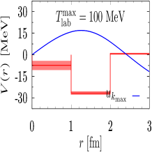
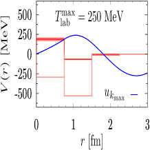
Figure 5: The evolution of the different square well potentials with the maximal fitting LAB energy. For illustration we also plot the maximum energy wave function in arbitrary units. The bifurcation between the repulsive and attractive core occurs at about $250$MeV.

IV.4 Evolution of potentials as a function of the fitting energy

In order to illustrate the coarse graining idea, we show in Fig. 4 the evolution of the phases as the maximal fitting energy is gradually increased in the repulsive core case. Essentially we just take as a guide that $\Delta r\sim 1/p_{\rm CM,max}$ and the number of square wells is approximately given by $N\sim r_{c}/\Delta r$. The errors are propagated from the fitting results beyond the fitting range. As we see, already with $N=5$ the prediction band contains the SAID data for which we plot both the real and the imaginary part of the phase-shift. A close study on the the evolution of the phases was carried out in a previous work RuizSimo:2016vsh taking the AV18 potential Wiringa:1994wb as a reference interaction which reproduces a fortiori the scattering data. There the coarse graining of the interaction with delta-shells was studied with similar conclusions. Here, besides using the square wells we also analyze the impact of phase-shift uncertainties stemming from the fits to the experimental data in the analysis. The evolution of the square well potentials as a function of the maximal fitting energy together with the corresponding wave function with the shortest wavelength are depicted in Fig. 5 illustrating the meaning of coarse graining in this particular case.

V Coarse grained Optical Potentials

We come now to the fit up to 3 GeV which, as mentioned above, is the largest LAB energy where a complete PWA has been undertaken and hence the particularly interesting ${}^{1}S_{0}$-wave has been extracted. Of course, at these high energies one may produce up to 7 pions among other particles, a circumstance that is beyond any comprehensive theoretical analysis at present due to the large number of coupled channels and multiparticles states. Therefore, and in line with previous developments and the discussion above we will use an optical potential. At the energies where the inelastic cross section is sizeable, relativistic corrections start playing a role. As mentioned above we will implement relativity invoking the invariant mass framework Allen:2000xy and already exploited in recent high energy studies Arriola:2016bxa .

Figure 6: Neutron-Proton Inelastic cross section as a function of the LAB energyLechanoineLeLuc:1993be . The $\Delta$ and $2\Delta$ resonance regions happen at $T_{\rm LAB}=0.64{\rm GeV}$ and $T_{\rm LAB}=1.36{\rm GeV}$ respectively.

Figure 7: Neutron-Proton inelasticity profile for the ${}^{1}S_{0}$ channel $1-\eta_{0}(b)^{2}$ as a function of the impact parameter $b=(l+1/2)/p$ for $l=0$ from the SAID database.

Figure 8: Fit to the real and imaginary part of the ${}^{1}S_{0}$ np SAID phase-shift as a function of the LAB energy up to 3 GeV for both the attractive and repulsive core cases (Top panel). Energy dependence of the ${\rm Re}V_{1}$ and ${\rm Im}V_{1}$ values keeping the remaining parameters to the energy independent values for the attractive core (middle panel) and the repulsive core (bottom panel). Continuous lines represent using the SAID solution and discretized lines represent direct determination from scattering data.

In general the coarse grained optical potential will be complex, and a pertinent question is what is the range of the inelasticity. We address this issue by noting that the inelastic cross section jumps from $\sigma_{\rm in}=1{\rm mb}$ to $\sigma_{\rm in}=28-32{\rm mb}$ in the CM range between $\sqrt{s}=2.3-2.7$GeV Ryan:1971rv (for a review see e.g. LechanoineLeLuc:1993be and references therein), which corresponds to nucleon resonance excitations $NN\to N\Delta$ or $NN\to\Delta\Delta$ for $M_{N}+M_{\Delta}\lesssim\sqrt{s}\lesssim 2M_{\Delta}$, i.e. $\sqrt{M\Delta}\lesssim p\lesssim\sqrt{2M\Delta}$ with $\Delta=M_{\Delta}-M_{N}$, and remains almost constant $\pm 1{\rm mb}$ up to 1000 GeV. We show as an illustration $\sigma_{\rm in}$ in Fig. 6 up to $3{\rm GeV}$ LAB energy. In the energy range we are concerned with $\sigma_{\rm in}\sim\sigma_{\rm el}$ so that the absorbing black disk picture holds. That means that the size of the hole is about 1fm. There are at least two ways to represent the absorptive S matrix, either as a complex phase-shift or as a real phase-shift and an inelasticity. The relation between both is

$$S_{l}(p)=\eta_{l}(p)e^{2i\delta_{l}(p)}=e^{-2\rho_{l}(p)}e^{2i\delta_{l}(p)}$$ (25)

On the other hand, the inelastic cross section can be written as a sum over partial waves,

$$\sigma_{\rm in}=\frac{\pi}{p^{2}}\sum_{l=0}^{\infty}(2l+1)\left[1-\eta_{l}(p)^{2}\right]$$ (26)

In the impact parameter representation where we can set $(l+1/2)=bp$, the S-wave involves the shortest impact parameter $b_{\rm min}=1/(2p)=1/\sqrt{s-4M^{2}}$ and at this level we can see from Fig. 7 that, $1-\eta_{0}(p)^{2}$ vanishes for $b$ larger than the coarse graining scale $\Delta r=0.3{\rm fm}$. Thus, we will assume just one complex and energy dependent fitting parameter for the innermost potential well, i.e. at $r=r_{1}\equiv\Delta r$,

$$V(r_{1},p) = {\rm Re}V(r_{1},p)+i{\rm Im}V(r_{1},p)\equiv{\rm Re}V_{1}+i{\rm Im}V_{1}$$ (27)

and keep the remaining $N-1$ points fixed and energy independent to the values of the previous fit at $T_{\rm LAB}=1{\rm GeV}$. The previous recursion relations, Eq. (15), hold also here by just replacing $\delta_{l}(p)\to\delta_{l}(p)+i\rho_{l}(p)$. The inelasticity and energy dependence at $r=r_{1}$ already improves the previous fit from $\chi^{2}/\nu=1.6$ to $\chi^{2}/\nu=0.7$.

Figure 9: Effect of switching off the imaginary part of the potential ${\rm Im}V_{1}=0$ keeping the remaining parameters in the ${}^{1}S_{0}$ np-phase-shift in the attractive and repulsive core scenarios.

Our procedure is as follows: for any energy value we fit the real and imaginary part of the phase shift following the strategy of taking just one complex and energy dependent parameter at the innermost sampling point. This will generate a discretized energy dependence of ${\rm Re}V(r_{1},p_{\alpha})$ and ${\rm Im}V(r_{1},p_{\alpha})$, with $T_{\rm LAB,\alpha}=2p_{\rm CM,\alpha}^{2}/M_{N}$ and $\alpha=1,\dots,N_{\rm Dat}$. In order to produce a smooth continuous curve we have also used the SAID solution which we find that it produces worse fits than the set of discretized energies.

The dependence of the innermost real and imaginary parts is depicted in Fig. 8 while the remaining components are kept energy independent from the previous low energy fit. As we can see the behavior is quite different. While in the attractive core case both ${\rm Re}V_{1}$ and ${\rm Im}V_{1}$ exhibit a rather smooth energy dependence, the repulsive core scenario presents a rapid and sudden change already in the region where the inelasticity is small. It is interesting to see what is the effect of switching off the inelastic contribution without refitting parameters. As we see in Fig. 9, the effect is dramatic in the standard repulsive core scenario and very mild in the attractive core case. Therefore, we can conclude that the inelastic contribution behaves truly as a perturbative effect in the structural core scenario.

VI Discussion and outlook

VI.1 The structural core and cluster models

Our finding for the repulsive branch echoes the result of G.E. Brown, 60 years ago brown1958proton namely a rapid and non-adiabatic transition from a repulsive core to an extremely absorbing disk. The underlying and microscopic reason why this sudden change might happen has never been clarified to our knowledge.

Unlike the repulsive branch, the attractive branch presents a deeply bound state at $E=-350{\rm MeV}$ already at the lowest LAB energy fits considered. This implies in particular that the zero energy wave function must have a node due to the oscillation theorem. In Fig. 2 (right) we show the zeroth energy wave function for both the attractive and repulsive branches in the 350 LAB energy fit case. As we see, they both vanish at short distances and feature the difference between the repulsive core, where the wave function vanishes below the core radius, and the structural core, where the wave function simply oscillates below the node. This pattern was already encountered in the OBE analysis and the main difference was taking an unnaturally large SU(3) violating $g_{\omega NN}\sim 20$ coupling constant or a natural one $g_{\omega NN}=3g_{\rho NN}\sim 10$ Cordon:2009pj . Here we confirm the trend when short distances are really probed by reproducing high energy scattering. The zero energy wave function pattern does not change much when the fitting energy is raised to $1{\rm GeV}$, as can be seen in Fig. 3. In Fig. 10 we show the shape of the deeply bound state for two maximal fitting energies corresponding to fit $n=5$ and $n=10$ wells.

Of course, this deeply bound state, while not influencing strongly the scattering, it would provide a very negative contribution to the binding energy in finite nuclei by just placing pairs of protons and neutrons in ${}^{1}S_{0}$ channel with the relative spurious bound state wave function. While at first sight this may seem an unsurmountable problem for the structural core scenario, in what follows we argue why this spurious deeply bound state could and should indeed be removed from the potential having no direct impact on the nuclear structure calculation.

Figure 10: Zero energy wave function and spurious Pauli-forbidden bound state when the fit is done with $n=5$ (left) and $n=10$ (right) square wells in the ${}^{1}S_{0}$ np-phase-shift in the attractive core scenario.

The argument is based on old considerations on the structural core Otsuki:1965yk ; TAMAGAKI:1967zz ; Otsuki:1969qu and they are most easily and beautifully exemplified by the discussion on ⁸Be made of two $\alpha$-clusters. Within a quark cluster model scheme for the nucleon, these nodes in the zero energy wave function are expected as a consequence of the Pauli principle of the constituent quarks, where not all quarks belonging to different nucleons are simultaneously exchanged, and hence is a more general requirement than the Pauli principle for nucleons.

One should note that the exact location of the node is searched within the standard cluster Gaussian wave function approach because for these states the CM can be easily extracted. A nice interpretation of the phenomenon can be given within the Saito orthogonality condition model which he analyzed thoroughly for two $\alpha$ clusters saito1969interaction ; saito1977chapter (for comprehensive reviews see e.g. tang1978resonating ; Friedrich:1981ad ) and we remind here briefly adapted to the nucleon-nucleon situation. Due to the total antisymmetry of the wave function, the interaction term between clusters contains a direct (Hartree) and an exchange (Fock) term, where the quarks inside one nucleon are exchanged with the quarks in another nucleon. For a local quark-quark interaction the direct nucleon-nucleon term is also local whereas the exchange term is nonlocal, and this is a short distance contribution which becomes negligible when the nucleons are at distances larger than their size. Thus, at large non-overlapping distances the direct and local term survives and one can work within a Hartree approximation. Within a Hartree-Fock framework Saito found that the Fock term had the effect of generating a node in the wave function when working in the Hartree approximation, i.e., when just the direct term is kept and the exchange term is ignored. Thus, there is no direct node-less zero energy wave function, since it is Pauli forbidden, and thus the corresponding deeply bound state which one finds in the Hartree approximation is spurious !. The Fock term generates the extra node of the wave function and prevents the nodeless wave function.

Our coarse grained potential corresponds to just using the direct term. Therefore, the node we find in the zero energy wave function is just a manifestation of the composite character of the nucleons when they are handled as if they were elementary. These views have been advocated in several papers Neudatchin:1975zz ; Neudachin:1977vt motivating the series of Moscow potentials Kukulin:1992vd .

VI.2 Extension to higher partial waves

The fact that coarse graining is working at these high energies in the case under study here with just S-wave is encouraging. It would thus be quite interesting to extend the analysis to higher partial waves, and actually it should be possible to make a complete coarse grained PWA using the delta-shells regularization extending previous work at about pion production threshold. Following the argument of a previous work Perez:2013cza we may count the total number of parameters by setting the maximal angular momentum $l_{\rm max}=p_{\rm max}r_{c}$ , and using $p_{\rm max}\Delta r\sim 1$. On the other hand, for any $l\leq l_{\rm max}$ we take $l(l+1)/r_{\rm min}=p_{\rm max}^{2}$. Thus we get using the $2\times 2$ spin-isospin degeneracy factor corresponding to neutron and proton states with spins up and down

$$N_{\rm par}=4\sum_{l=0}^{l_{\rm max}}\sum_{n}\theta\left(p^{2}-\frac{l(l+1)}{r_{n}^{2}}\right)\sim 4\frac{1}{2}(p_{\rm max}r_{c})^{2}$$ (28)

For the studied case here where $r_{c}=3{\rm fm}$ and $T_{\rm LAB}=3{\rm GeV}$ , i.e. $p_{\rm CM}=1.26{\rm GeV}$ one gets $N_{\rm par}\sim 700$, or equivalently $N_{\rm par}^{pp}=N_{\rm par}^{nn}\sim 175$ and $N_{\rm par}^{pn}\sim 350$. These are large numbers of parameters, but not very different from the ones needed in the comprehensive most recent SAID np fit Workman:2016ysf based on a parameterization Arndt:1986jb with a total number of 147 parameters. It remains to be seen if these extra parameters might perhaps improve the quality of these fits since they describe $25362$-pp data with $\chi^{2}=48780.934$ and $13033$-np data with $\chi^{2}=26261.000$.

VI.3 Implications for nuclear physics

Fitting NN scattering data is not only a possible way to represent the data, but also the fitted potential is meant to be used in a nuclear structure calculation. While this seems most obvious, the well known complexities of the nuclear many-body problem require making a choice on the characteristics features of the potential itself. For instance, the mere concept of a repulsive core requires considering a local potential. This particular form is best suited for MonteCarlo type calculations and underlies the Argonne potentials saga Lagaris:1981mm ; Wiringa:1984tg ; Wiringa:1994wb . Nonlocal or velocity dependent potentials do not exhibit the repulsive core so explicitly  and are usually handled by other techniques, such as no-core shell model.

On the other hand, if we want to access to the short distance region in finite nuclei by say, knock out processes (e,e’,NN), we must fix the NN interaction going to high enough energies where both inelasticities and relativity ought to be important ingredients of the calculation. The resulting interaction, such as the one determined in the present paper, will thus become complex and energy dependent, and it is unclear at present how to use such an interaction in conventional Nuclear Structure calculations from an ab initio point of view where the main assumption is to take real and energy independent potentials. We hope to address these issues in the future.

VI.4 Implications for Hadronic Physics

The fact that the coarse graining approach works for NN scattering in a regime where relativistic and inelastic effects become important suggests extending the method to other hadronic reactions under similar operating conditions such as $\pi\pi$ scattering up to $\sqrt{s}=1.4{\rm GeV}$ jacobo2017 . Within such a context the methods based in analyticity, dispersion relations and crossing are currently considered to be, besides QCD, the most rigorous framework (See e.g. Ananthanarayan:2000ht ; GarciaMartin:2011cn and references therein). We stress that such an approach is based on the validity of the double spectral representation of the four-point function conjectured by Mandelstam. It is noteworthy that under this same assumption the optical potential of the form used in the present paper was derived many years ago cornwall1962mandelstam ; omnes1965optical ; analytic properties for $V(r,s)$ in the $s$-variable in the form of a dispersion relation at fixed relative distance $r$ were deduced. Due to their linear character dispersion relations would be preserved under the coarse graining operation at the grid points for $V(r_{i},s)$. In the present paper we have considered $NN$ taking both real and imaginary parts of the optical potential as independent variables. A much better procedure would be to constrain our fit to satisfy the fixed-r dispersion relations. This interesting study would require some sound assumptions on the interaction at high energies and is left for future research.

VII Conclusions

We summarize our points. The repulsive nuclear core is a short distance feature of the NN interaction which has been the paradigm in Nuclear Physics for many years. This allows not only to explain nuclear and neutron matter stability at sufficiently high densities, but also many realistic and successful ab initio calculations implement this repulsive core view, providing a compelling picture of short-range correlations and even lattice QCD calculations seem to provide evidence on the repulsive core.

In this work we have tried to verify the paradigm by analyzing directly scattering data in a model independent way up to energies corresponding to a wavelength short enough to separate the well established core region from the rest of the potential. We have also critically analyzed recent evidence provided by lattice QCD calculations of NN potentials and seemingly supporting the repulsive core scenario. On the light of the avoiding crossing phenomenon triggered by multipion creation and disregarded in the lattice calculations the repulsive core is just un upper bound of the true energy, and not a genuine feature of the NN interaction.

A coarse grained optical potential approach has been invoked implementing a Wilsonian re-normalization point of view. This is based in sampling the interaction with a complex potential at points separated by a sampling resolution corresponding to the minimal de Broglie wavelength, $\Delta r\sim 1/p_{\rm CM}$, for a given CM-momentum, $p_{\rm CM}$. The number of sampling points is determined from the range of the region where the interaction is unknown. We assume, in agreement with previous low energy studies scanning the full database of np+pp about pion production threshold, that the interaction above $r_{c}=3$fm is given by the One-Pion-Exchange potential and sample the interaction at equidistant points separated by the resolution scale $\Delta r$.

Traditionally, the core region is estimated to be around $a_{c}\sim 0.5$ fm. This requires considering LAB energies up to about 3 GeV, for which there exist comprehensive partial wave analyses. Since, the ${}^{1}S_{0}$ partial wave explores the shortest impact parameter $b\sim 1/(2p_{\rm CM})$, we have mainly restricted our analysis to this channel and have shown that the inelasticity is concentrated in a region below the resolution scale $\Delta r$. This amounts to treat the inelasticity interaction as point-like and structure-less. In the coarse grained setup, that means that we treat only the potential at the innermost sampling distance as complex and energy dependent. The remaining sampling points are kept real and energy independent. We have shown successful fits describing the real and imaginary parts of the ${}^{1}S_{0}$ phase-shift up to 3 GeV LAB energy. However, two conflicting scenarios emerge from these fits where the interaction at short distances becomes either strongly repulsive (the repulsive core) or strongly attractive (the structural core). Both scenarios have been considered in the past as alternative pictures of the NN interaction at short distances and here we show explicitly how both arise from a similar way of sampling the interaction with a coarse grained potential. We corroborate the main difference between both scenarios concerning the zero energy wave function which vanishes below the core distance in the repulsive core case and has a node at about the core location but does not vanish below it in the structural core situation. Since these two scenarios are phase-equivalent, we have analyzed in a comparative way some of their features addressing the obvious question on which one is more realistic.

There is a remarkable and tangible difference between the short distance repulsive-core and the structural-core core scenarios, namely, the adiabaticity of the inelasticity. In the repulsive core case we get a rapid variation between a very strong short distance repulsion and a very strong absorption. In contrast, in the structural core situation, the behavior is completely smooth, and the inelasticity couples in an adiabatic way as the energy is steadily increased.

On the other hand, while the repulsive core has no bound states, in agreement with experiment, the structural core presents a deeply bound state which might pose a problem for nuclear structure calculations. Cluster model studies have suggested that this deeply bound state is forbidden by the Pauli principle for the underlying quarks and the node in the wave function is just a manifestation of the composite character of the nucleons. In fact, our way of solving the problem using an effective interaction at the hadronic level corresponds at the sub-nucleon level to consider just the direct Hartree term, whereas the exchange Fock term generates naturally the node of the relative wave function without the spurious bound state. The repulsive core branch presents a dramatic change from the core to a strongly absorbing potential for which we are not aware of any microscopic explanation.

An interesting application is the study of nuclear processes where two particles are emitted at high relative momentum and the implications for our understanding of short distance correlations since most studies in Nuclear Physics ignore the role of inelasticities when fixing the interaction at high energies. The fruitfulness of the coarse graining idea has been demonstrated recently in an efficient solution method of the Bethe-Goldstone equation and the presently obtained wave functions could be used to study the effects of inelasticity on short-range correlations, a task that has never been addressed, and is left for future research.

Finally, the present study shows that the coarse graining idea works as expected at LAB energies as high as 3 GeV where the consideration of inelasticities is unavoidable, and suggest to extend the present calculation to higher partial waves or other hadronic processes.

One of us (E.R.A.) thanks David R. Entem for discussions on quark cluster models. We thank Jacobo Ruiz de Elvira, Quique Amaro and Eulogio Oset for discussions and for critically reading the ms.

This work is supported by the Spanish Ministerio de Economía y Competitividad and European FEDER funds under contract FIS2014-59386-P, FIS2014-51948-C2-1-P and by Junta Andalucía (grant FQM225). P. F.-S. acknowledges financial support from the “Ayudas para contratos predoctorales para la formación de doctores” program (BES-2015-072049) from the Spanish MINECO and ESF.

References

- (1) R. Jastrow, Phys. Rev. 81 (1951) 165.
- (2) G.E. Brown, Physical Review 111 (1958) 1178.
- (3) M.A. Preston and R.K. Bhaduri, Structure of the Nucleus (Elsevier, 1975).
- (4) T. Hamada and I.D. Johnston, Nucl. Phys. 34 (1962) 382.
- (5) R.V. Reid, Jr., Annals Phys. 50 (1968) 411.
- (6) R. Tamagaki, Prog. Theor. Phys. 39 (1968) 91.
- (7) S. Otsuki, Prog. Theor. Phys. Suppl. 42 (1969) 39.
- (8) H. Bethe, Nuclear Matter (Academic Press, New York and London, 1970).
- (9) R. Machleidt, Adv. Nucl. Phys. 19 (1989) 189.
- (10) I.E. Lagaris and V.R. Pandharipande, Nucl. Phys. A359 (1981) 331.
- (11) R.B. Wiringa, R.A. Smith and T.L. Ainsworth, Phys. Rev. C29 (1984) 1207.
- (12) R.B. Wiringa, V.G.J. Stoks and R. Schiavilla, Phys. Rev. C51 (1995) 38, nucl-th/9408016.
- (13) S.C. Pieper and R.B. Wiringa, Ann. Rev. Nucl. Part. Sci. 51 (2001) 53, nucl-th/0103005.
- (14) J. Carlson et al., Rev. Mod. Phys. 87 (2015) 1067, 1412.3081.
- (15) Y. Nambu, Phys. Rev. 106 (1957) 1366.
- (16) R.A. Bryan and B.L. Scott, Phys. Rev. 135 (1964) B434.
- (17) R. Machleidt, Phys. Rev. C63 (2001) 024001, nucl-th/0006014.
- (18) E. Oset, H. Toki, M. Mizobe and T. T. Takahashi, Prog. Theor. Phys. 103, 351 (2000)
- (19) F. Gross, Phys. Rev. D10 (1974) 223.
- (20) S. Otsuki, M. Yasuno and R. Tamagaki, Prog. Theor. Phys. Suppl. E65 (1965) 578.
- (21) R. Tamagaki, Rev. Mod. Phys. 39 (1967) 629.
- (22) V.G. Neudatchin et al., Phys. Rev. C11 (1975) 128.
- (23) V.G. Neudachin, Yu.F. Smirnov and R. Tamagaki, Prog. Theor. Phys. 58 (1977) 1072.
- (24) V.I. Kukulin and V.N. Pomerantsev, Prog. Theor. Phys. 88 (1992) 159.
- (25) V.G. Neudachin et al., Phys. Rev. C43 (1991) 2499.
- (26) V.I. Kukulin and M.N. Platonova, Phys. Atom. Nucl. 76 (2013) 1465, [Yad. Fiz.76,1549(2013)].
- (27) A. Calle Cordon and E. Ruiz Arriola, Phys. Rev. C81 (2010) 044002, 0905.4933.
- (28) Sinya AOKI for HAL QCD, S. Aoki, Prog. Part. Nucl. Phys. 66 (2011) 687, 1107.1284.
- (29) S. Aoki, Eur. Phys. J. A49 (2013) 81, 1309.4150.
- (30) S. Aoki, J. Balog and P. Weisz, Prog. Theor. Phys. 128 (2012) 1269, 1208.1530.
- (31) L.D. Landau and E.M. Lifshits, Quantum Mechanics Non-relativistic Theory: Transl. from the Russian by JB Sykes and JS bell. 2d Ed., rev. and Enl (Pergamon Press, 1965).
- (32) C. Lechanoine-LeLuc and F. Lehar, Rev. Mod. Phys. 65 (1993) 47.
- (33) J. Ball et al., Eur. Phys. J. C5 (1998) 57.
- (34) J. Bystricky, F. Lehar and C. Lechanoine-LeLuc, Eur. Phys. J. C4 (1998) 607.
- (35) J. Ball et al., Nuovo Cim. A111 (1998) 13.
- (36) R.A. Arndt et al., Phys. Rev. D28 (1983) 97.
- (37) R.A. Arndt, J.S. Hyslop, III and L.D. Roper, Phys. Rev. D35 (1987) 128.
- (38) R.A. Arndt et al., Phys. Rev. D45 (1992) 3995.
- (39) R.A. Arndt et al., Phys. Rev. C56 (1997) 3005, nucl-th/9706003.
- (40) R.A. Arndt, I.I. Strakovsky and R.L. Workman, Phys. Rev. C62 (2000) 034005, nucl-th/0004039.
- (41) R.A. Arndt et al., Phys. Rev. C76 (2007) 025209, 0706.2195.
- (42) . http://gwdac.phys.gwu.edu, Center For Nuclear Studies. Data Analysis center. N-N interaction .
- (43) R.L. Workman, W.J. Briscoe and I.I. Strakovsky, Phys. Rev. C94 (2016) 065203, 1609.01741.
- (44) R. Shneor et al. [Jefferson Lab Hall A Collaboration], Phys. Rev. Lett. 99, 072501 (2007)
- (45) H. Feldmeier, W. Horiuchi, T. Neff and Y. Suzuki, Phys. Rev. C 84, 054003 (2011)
- (46) M. Vanhalst, J. Ryckebusch and W. Cosyn, Phys. Rev. C 86, 044619 (2012)
- (47) M. Alvioli, C. Ciofi Degli Atti, L. P. Kaptari, C. B. Mezzetti and H. Morita, Int. J. Mod. Phys. E 22, 1330021 (2013)
- (48) R. B. Wiringa, R. Schiavilla, S. C. Pieper and J. Carlson, Phys. Rev. C 89, no. 2, 024305 (2014) doi:10.1103/PhysRevC.89.024305 [arXiv:1309.3794 [nucl-th]].
- (49) I. Ruiz Simo et al., (2016), 1612.06228.
- (50) EDDA, K.O. Eyser, R. Machleidt and W. Scobel, Eur. Phys. J. A22 (2004) 105, nucl-th/0311002.
- (51) T.W. Allen, G.L. Payne and W.N. Polyzou, Phys. Rev. C62 (2000) 054002, nucl-th/0005062.
- (52) H. Feshbach, Annals Phys. 5 (1958) 357.
- (53) H. Feshbach, Annals Phys. 19 (1962) 287, [Annals Phys.281,519(2000)].
- (54) J.M. Cornwall and M.A. Ruderman, Physical Review 128 (1962) 1474.
- (55) R. Omnes, Physical Review 137 (1965) B653.
- (56) T. Ueda, M.L. Nack and A.E.S. Green, Phys. Rev. C8 (1973) 2061.
- (57) S.G. Bondarenko et al., Nucl. Phys. A832 (2010) 233, 0810.4470.
- (58) S.G. Bondarenko, V.V. Burov and E.P. Rogochaya, Phys. Lett. B705 (2011) 264.
- (59) E. Ruiz Arriola and W. Broniowski, Few Body Syst. 57 (2016) 485, 1602.00288.
- (60) E. Ruiz Arriola and W. Broniowski, Phys. Rev. D95 (2017) 074030, 1609.05597.
- (61) D.R. Entem et al., Phys. Rev. C77 (2008) 044006, 0709.2770.
- (62) R. Navarro Perez, J.E. Amaro and E. Ruiz Arriola, Prog. Part. Nucl. Phys. 67 (2012) 359, 1111.4328.
- (63) R. Navarro Perez, J.E. Amaro and E. Ruiz Arriola, Few Body Syst. 54 (2013) 1487, 1209.6269.
- (64) R. Navarro Pérez, J. E. Amaro and E. Ruiz Arriola, Phys. Rev. C 88, no. 6, 064002 (2013) Erratum: [Phys. Rev. C 91, no. 2, 029901 (2015)]
- (65) R. Navarro Perez, J.E. Amaro and E. Ruiz Arriola, Few Body Syst. 55 (2014) 983, 1310.8167.
- (66) R. Navarro Pérez, J.E. Amaro and E. Ruiz Arriola, Phys. Lett. B724 (2013) 138, 1202.2689.
- (67) K. Chadan and P. Sabatier, Inverse Problems in Quantum Scattering Theory. 1989 (Springer-Verlag).
- (68) H. Leeb, H. Fiedeldey and R. Lipperheide, Phys. Rev. C32 (1985) 1223.
- (69) N.A. Khokhlov and V.A. Knyr, (2004), nucl-th/0410092.
- (70) H.V. von Geramb et al., Phys. Rev. C58 (1998) 1948, nucl-th/9803031.
- (71) A. Funk, H.V. von Geramb and K.A. Amos, Phys. Rev. C64 (2001) 054003, nucl-th/0105011.
- (72) V.A. Knyr, V.G. Neudachin and N.A. Khokhlov, Phys. Atom. Nucl. 69 (2006) 2034, [Yad. Fiz.69,2079(2006)].
- (73) N.A. Khokhlov and V.A. Knyr, Phys. Rev. C73 (2006) 024004, quant-ph/0506014.
- (74) K.A. Wendt, R.J. Furnstahl and S. Ramanan, Phys. Rev. C86 (2012) 014003, 1203.5993.
- (75) J.B. Aviles, Phys. Rev. C6 (1972) 1467.
- (76) S. Albeverio et al., Journal of Mathematical Physics 54 (2013) 052103.
- (77) R.N. Perez, J.E. Amaro and E. Ruiz Arriola, (2016), 1606.00592.
- (78) A. Sibirtsev et al., Eur. Phys. J. A45 (2010) 357, 0911.4637.
- (79) W.P. Ford and J.W. Van Orden, Phys. Rev. C87 (2013) 014004, 1210.2648.
- (80) R. Navarro Perez, J.E. Amaro and E. Ruiz Arriola, Phys. Rev. C89 (2014) 064006, 1404.0314.
- (81) E. Oset and L.L. Salcedo, J. Comput. Phys. 57 (1985) 361.
- (82) R. Navarro Pérez, E. Ruiz Arriola and J. Ruiz de Elvira, Phys. Rev. D91 (2015) 074014, 1502.03361.
- (83) R. Navarro Pérez, J.E. Amaro and E. Ruiz Arriola, Phys. Lett. B738 (2014) 155, 1407.3937.
- (84) B.A. Ryan et al., Phys. Rev. D3 (1971) 1.
- (85) S. Saito, Progress of Theoretical Physics 41 (1969) 705.
- (86) S. Saito, Progress of Theoretical Physics Supplement 62 (1977) 11.
- (87) Y.C. Tang, M. LeMere and D. Thompsom, Physics Reports 47 (1978) 167.
- (88) H. Friedrich, Phys. Rept. 74 (1981) 211.
- (89) T. Neff, H. Feldmeier and W. Horiuchi, Phys. Rev. C 92, no. 2, 024003 (2015)
- (90) J. Ruiz de Elvira and E. Ruiz Arriola, In preparation (2017).
- (91) B. Ananthanarayan et al., Phys. Rept. 353 (2001) 207, hep-ph/0005297.
- (92) R. Garcia-Martin et al., Phys. Rev. D83 (2011) 074004, 1102.2183.