Abstract:

We present the computer code RECOLA2 along with the first NLO electroweak corrections to Higgs production in vector-boson fusion and updated results for Higgs strahlung in the Two-Higgs-Doublet Model and Higgs-Singlet extension of the Standard Model. A fully automated procedure for the generation of tree-level and one-loop matrix elements in general models, including renormalization, is presented. We discuss the application of the Background-Field Method to the extended models. Numerical results for NLO electroweak cross sections are presented for different renormalization schemes in the Two-Higgs-Doublet Model and the Higgs-Singlet extension of the Standard Model. Finally, we present distributions for the production of a heavy Higgs boson.

1 Introduction

Since the discovery of a Higgs boson at the Large Hadron Collider (LHC) [1, 2] the community is moving forward focusing on precision. Precision is the key to probe the Standard Model (SM) and Beyond Standard Model (BSM) physics and potentially allows, together with automation, to disprove the SM or even to single out new models. State of the art predictions involve typically two-loop and occasionally three-loop $\mathrm{QCD}$ and one-loop electroweak ($\mathrm{EW}$) corrections for many processes of interest at the LHC. As the aim is to cover all accessible processes at the LHC and future colliders, a lot of effort has gone into the full automation of one-loop amplitudes. With one-loop $\mathrm{QCD}$ amplitudes being available since a long time, more recently much effort has been spent on the automation of $\mathrm{EW}$ one-loop corrections, which are more important than ever in view of the recent progress in multi-loop $\mathrm{QCD}$ calculations. SM $\mathrm{EW}$ corrections are nowadays available in various approaches, e.g. OpenLoops[3], MadGraph5_aMC@NLO[4], GoSam[5, 6], FeynArts/FormCalc[7, 8], and in our fully recursive approach RECOLA[9, 10]. For BSM physics precision is important, and especially $\mathrm{EW}$ corrections should not be underestimated as they can be comparable to $\mathrm{QCD}$ corrections in certain BSM scenarios.

The automation for one-loop BSM physics requires three ingredients: First, new models need to be defined, typically in form of a Lagrangian and followed by the computation of the Feynman rules. For this kind of task Feynrules[11] and SARAH[12] are established tools. Then, a systematic and yet flexible approach to the renormalization and computation of further ingredients is required to deal with generic models. Finally, the renormalized model file needs to be interfaced to a generic one-loop matrix-element generator. As for the automation of renormalization, there has been progress in the Feynrules/FeynArts approach[13]. In this paper we present an alternative and fully automated procedure to the renormalization and computation of amplitudes in general models, thus, combining the second and third step. Our approach makes use of tree-level Universal FeynRules Output (UFO) model files[14] and results in renormalized one-loop model files for RECOLA2, a generalized version of RECOLA, allowing for the computation of any process in the underlying theory at the one-loop level, with limitations only due to available memory or CPU workload.

As an application of the system, we focus on two BSM Higgs-production processes at the LHC, namely Higgs production in association with a vector boson, usually referred to as Higgs strahlung, and Higgs production in association with two jets, known as vector-boson fusion (VBF), in the Two-Higgs-Doublet Model (2HDM) and the Higgs-Singlet extension of the SM (HSESM). Those processes are particularly interesting for an extended Higgs sector, as they represent the next-to-most-dominant Higgs-production mechanisms at the LHC. There has been enormous progress in higher-order calculations to Higgs strahlung and VBF in the SM and BSM. For Higgs strahlung the $\mathrm{QCD}$ corrections are known up to NNLO for inclusive[15, 16, 17] and differential [18, 19] cross sections. On-shell $\mathrm{EW}$ corrections were computed in Ref. [20] and followed by the off-shell calculation in Ref. [21]. Higgs strahlung has also been investigated in the 2HDM for $\mathrm{QCD}$ [22] and $\mathrm{EW}$[23] corrections. NLO QCD corrections matched to parton shower have been presented in Ref. [24] in an effective field theory framework. For VBF, the first one-loop $\mathrm{QCD}$ corrections were obtained in a structure function approach[25] followed by the first two-loop prediction[26, 27] in the same framework. As for differential results, the first one-loop $\mathrm{QCD}$ and $\mathrm{EW}$ corrections were calculated in Ref. [28] and Refs. [29, 30], respectively. Since recently also the differential two-loop[31] and three-loop[32] $\mathrm{QCD}$ corrections are available. VBF has been interfaced to parton showers[33, 34] and has been subject to studies for a 100 TeV collider[35]. In view of BSM, VBF has been studied in the MSSM[36]. Higgs strahlung and VBF are nowadays available in public codes, such as V2HV [37], MCFM [38], HAWK2.0 [39] and vh@nnlo [40].

This paper is organized as follows. In Section 2 the computer program RECOLA2 is presented as a systematic approach towards the automated generation of one-loop processes. RECOLA2 relies on one-loop renormalized model files which are automatically generated with the new tool REPT1L from nothing but Feynman rules. The computation steps are explained in different subsections, where we discuss the translation from UFO to RECOLA2 model files (Section 2.1), the counterterm expansion and renormalization, and the computation of rational terms of type $R_{2}$ (Section 2.2). In Section 3 we give details on the HAWK 2.0 interface with RECOLA2, which has been used for the phenomenology. In Section 4 we list our conventions for the 2HDM and the HSESM, focusing on the physical input parameters. In Section 5 we discuss the application of the Background-Field Method (BFM) in RECOLA2. We present the renormalization for extended Higgs sectors in the BFM and give details on the implementation in REPT1L. In Section 6 we fix the calculational setup and define the benchmark points, which were mainly taken from the Higgs cross section working group (HXSWG). For the numerical analysis we use different renormalization conditions for the mixing angles, which we introduce in Section 6.3. In Section 7 we present the numerical results, discussing total cross sections in view of different renormalization schemes and distributions for heavy Higgs-boson production. After the conclusions in Section 8, we illustrate in App. A how the colour flow is derived and provide additional information on the derivation of a minimal basis for off-shell currents in App. B. Finally, in App. C we discuss the application of on-shell renormalization schemes combined with different tadpole counterterm schemes focusing on the gauge dependence.

2 RECOLA2: RECOLA for general models

RECOLA2 is a tree-level and one-loop matrix-element provider for general models involving scalars, fermions and vector particles. It is based on its predecessor RECOLA[9, 10], which uses Dyson–Schwinger equations [41, 42, 43] to compute matrix elements in a fully numerical and recursive approach. The implementation at tree level follows the strategy developed in Ref. [44], supplemented by a special treatment of the colour algebra. The one-loop extension, inspired by Ref. [45], relies on the decomposition of one-loop amplitudes as linear combination of tensor integrals and tensor coefficients. The former are evaluated by means of the library COLLIER[46], while the latter can be computed by making use of similar recursion relations as for tree amplitudes. The key point is the construction of the proper tensor structure of the coefficients at each step of the recursive procedure, which has been implemented in RECOLA relying on the fact that in the Standard Model in the ’t Hooft–Feynman gauge the combination (vertex)$\times$(propagator) is at most linear in the momenta. RECOLA2 circumvents these and other limitations of RECOLA. In the following we give an introduction to RECOLA2 and its capabilities, focusing on the generalization with respect to RECOLA and on the applications presented in Section 7.

The generalization of RECOLA has required to remove all SM-based pieces of code, replacing them with generic structures which are able to retrieve any necessary information from the model file. Furthermore, the process-generation algorithm makes use of recursive functions dealing with different cases on equal footing. This has produced a more compact code as no model-dependent information has been hard-coded. Finally, RECOLA2 just needs the Feynman rules to be provided by model files in a specific format to directly evaluate NLO amplitudes in the model under consideration by using similar recursion relations to those of the SM. As for RECOLA, the key ingredients are the so-called off-shell currents

$$w^{i}(P,\{n\})=\raisebox{-11.99998pt}{ \includegraphics{pics/current} }$$ (2.1)

defined as the sum of all Feynman graphs which generate the off-shell particle $P$ combining $n$ external particles. The generic index $i$ is related to the spin. For example, in the case of a vector field $i$ is a Lorentz index or in the case of a fermionic field $i$ is a spinor index. Other indices are suppressed and not relevant for the following discussions.

The off-shell currents (2.1) are build recursively according to the Berends–Giele recursion relations (BGR) [47]

$$\raisebox{-43.00009pt}{ \includegraphics{pics/BGR} },$$ (2.2)

which constitute a generalization of Eq. (2.2) of Ref. [9] for general models where elementary couplings with more than four fields are present. Note that in RECOLA [10] the terms with $\lambda_{i}$, $i>4$ are absent as only 2-, 3-, and 4-point interaction vertices are supported. Practically, each term on the right-hand side of the $\mathrm{BGR}$ equation (2.2) combines off-shell currents, referred to as incoming currents, and contributes to the construction of the current on the left-hand side, referred to as outgoing current. An outgoing off-shell current with $n$ external particles is calculated using the vertices of the theory connecting incoming off-shell currents with less than $n$ external particles, which, when combined, add up to $n$ external particles. This can be realized for tri-linear, quadri-linear, quinti-linear, or even higher $n$-point vertices if present in the theory. The contribution to the outgoing current generated in each term of equation (2.2) can be formally seen as the result of the action of the $\mathrm{BGR}$ operator defined by

$$\raisebox{-34.50002pt}{ \includegraphics{pics/wout} }\quad\Rightarrow\quad w_{\mathrm{Out}}=\sum\mathrm{BGR}\left(w_{\mathrm{In,1}},\ldots w_{\mathrm{In,N}}\right),$$ (2.3)

with the sum running over all contributions in (2.2).

The equations (2.2) and (2.3) can be written in a model-independent way as a linear combination of Lorentz structures from which the couplings, colour structures and other relevant information that needs to be propagated from the left to the right is factorized. RECOLA2 is fully relying on the model file to provide those rules, in addition to recursive rules for the colour-flow and helicity-state propagation. One could argue, that not too many different operators are required, at least for the renormalizable theories, which could have been hard-coded. However, in view of different conventions, different gauges and non-renormalizable theories, we decided for a flexible system by moving this dependence to the model file. As now the model file provides the rules for computing off-shell currents, we can easily incorporate the BFM and $\mathrm{R}_{\xi}$-gauge for the SM and BSM models for $\mathrm{NLO}$ computations which is discussed in Section 5. In addition, RECOLA2 has been generalized to deal with arbitrary $n$-point vertices, and, thus, can compute processes with elementary interactions between more than four fields. Dealing with higher $n$-point vertices required to improve, among other parts of the code, the generation of the tree graphs of the process. The generation of those graphs is a combinatorial problem which is practically solved in the binary representation as introduced in Ref. [48] (see also Ref. [44]). For elementary interactions involving an arbitrary number of fields the method requires to compute distinct ordered integer partitions of arbitrary size with no bitwise overlap between elements.

Further, RECOLA2 allows for arbitrary powers of momenta in Feynman rules, which is crucial for EFTs and the $\mathrm{R}_{\xi}$-gauge at one-loop level. In order to implement this important generalization, we had to generalize the construction of the tensor structure of loop currents (i.e. of the coefficients of the tensor integrals), allowing the combination (vertex)$\times$(propagator) to contain any power of momenta.

New theories may involve new fundamental couplings, and RECOLA2 can deal with an arbitrary number of them. The computation of matrix elements is ordered according to powers of fundamental couplings, and RECOLA2 provides methods to automatically compute amplitudes and interferences for all possible orders of these couplings. For instance, this feature can be used to control the number of insertions of a higher dimensional operator in a given amplitude.

Finally, RECOLA2 comes with almost all features and optimizations as provided by RECOLA. It is designed to be backward compatible in the sense that a program which successfully runs with RECOLA can be linked to RECOLA2 and a SM (or SM BFM) model file and is guaranteed to run without any code adaptation. This is realized by a dedicated SM interface which has been developed on top of the general interface to model files. The most notable optimizations concern partial factorization in colour-flow representation, the use of helicity conservation and the identification of fermion loops for different fermions with equal masses.

2.1 RECOLA2 model-file generation

RECOLA2 model files are generated with the tool REPT1L (Recola’s rEnormalization Procedure Tool at 1 Loop) which is a multi-purpose tool for analytic computations at the one-loop order. REPT1L is written in Python 2.7 and depends on other tools, most notably RECOLA2 for the model-independent current generation, which is used in combination with FORM[49] to construct analytic vertex functions or $S$-matrix elements, and SymPy[50], which is a computer-algebra system (CAS) for Python.

REPT1L requires the Feynman rules in the UFO format [14] which can be derived via Feynrules[11] or SARAH[12]. As there has been progress for an automated renormalization in the Feynrules framework [13], we stress that we do not require any results for counterterms or rational terms. Those terms are automatically derived from the tree-level Feynman rules in a self-contained fashion as explained in Section 2.2.

The RECOLA2 model-file generation consists of two phases. In the first phase REPT1L loops over all vertices in the UFO model file, disassembling each into the vertex particles, Lorentz and colour structures, and couplings. The colour structure is transformed to the colour-flow basis possibly rearranging Lorentz structures and couplings. This is discussed in more detail in App. A. The resulting Lorentz structures are used to derive the $\mathrm{BGR}$ operators in a model-independent way. For every Feynman rule REPT1L tries to map the encountered Lorentz structure onto one of those operators. If a new structure cannot be mapped onto an existing operator a new operator is added. In an optional second pass, the existing base of operators is minimized (see App. B for more details).

In the second phase of the model-file generation the information is exported as Fortran95 code in form of a model-file library as depicted in Fig. 1. Particle configurations are linked to the individual contributions on the right-hand side of (2.2), which differ in the underlying $\mathrm{BGR}$ (2.3), colour flow, colour factors, couplings, coupling orders or other information, via a Fortran95 hash table, allowing for a flexible and efficient access. The actual $\mathrm{BGR}$ are computed and exported as Fortran95 subroutines in different forms. For the numerical evaluation tree and loop $\mathrm{BGR}$ are used to construct tree-level and one-loop amplitudes as it is done in RECOLA. The tree $\mathrm{BGR}$ are a special case of the loop $\mathrm{BGR}$, with no loop-momentum dependence. As a new feature in RECOLA2, an analytic version of the $\mathrm{BGR}$ allows to generate amplitudes as FORM code. In this way the analytic expressions for the amplitudes needed in the renormalization conditions are derived in the same framework as the loop amplitudes of the computed processes, ensuring that properly defined renormalization schemes automatically imply UV-finite results in numerical computations. In general, the UV finiteness of the theory can (and should) be verified numerically in RECOLA2 process by process by varying the scale $\mu_{\mathrm{UV}}$ related to the dimensional regularization of UV singularities [10]. This check also works in combination with ${\overline{\mathrm{MS}}}$ subtraction schemes, even though in this case amplitudes have an intrinsic scale dependence. To this end, we separate the scale dependence originating from the ${\overline{\mathrm{MS}}}$ subtraction from the one of regularization.

Finally, RECOLA2 requires particle information such as the mass, spin, and colour of particles. This information is directly obtained from UFO particle instances and is translated to Fortran95 code.

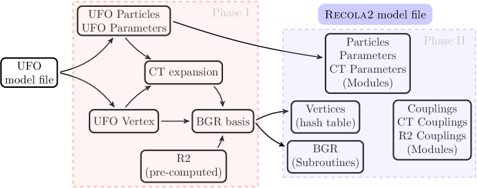
Figure 1: The RECOLA2 model-file generation. UFO vertices are taken as input and each vertex is permuted and mapped to a suited $\mathrm{BGR}$ operator. Given a counterterm expansion (2.4), REPT1L can generate all counterterm vertices and include them in the $\mathrm{BGR}$. Once the renormalization is done and the $R_{2}$-terms are computed, the model file is derived once again, including solutions to counterterm parameters and $R_{2}$ terms.

These steps conclude the tree-level model-file generation. In the next section we discuss the counterterm generation and renormalization and the computation of rational terms of type $R_{2}$.

2.2 Counterterm expansion, renormalization and computation of $R_{2}$ terms

REPT1L supports an automated renormalization of model files following the standard procedure (see e.g. Ref. [51]). Here we give a short summary of all the steps, followed by details on the counterterm expansion, the renormalization conditions, and the computation of rational terms of type $R_{2}$.

The starting point is a tree-level UFO model file. In the first step an independent set of parameters is identified, followed by a counterterm expansion. The RECOLA2 model file is derived, enabling the formal counterterm expansion in REPT1L and leaving the values for counterterm parameters unspecified. Renormalization conditions are used to fix the counterterm parameters. REPT1L allows to renormalize counterterm parameters in various schemes, and specific schemes are selected at run-time in RECOLA2. The rational terms of type $R_{2}$ are constructed from vertex functions of the underlying theory. The model file is derived once again, including the counterterm expansion, solutions to counterterm parameters and $R_{2}$ terms. The result is the desired renormalized model file, ready for computation of processes supported by the underlying theory.

Counterterm expansion

In the default setup, REPT1L defines the counterterm expansion rules of the masses $M_{V}$, $M_{S}$, $m_{f}$, associated to scalars ($S$), vector bosons ($V$) and fermions ($f$), of the not necessarily physical bosonic ($\phi$) and fermionic fields ($\psi$), and of a set of external couplings $g_{k}$, according to

$$M_{V}^{2}\to M_{V}^{2}+\delta M_{V}^{2},\quad M_{S}^{2}\to M_{S}^{2}+\delta M_{S}^{2},\quad m_{f}\to m_{f}+\delta m_{f},$$

$$\phi_{j}\to\sum_{l}\left(\delta_{jl}+\frac{1}{2}\delta Z_{jl}\right)\phi_{l},\quad \psi^{\rm L}_{i}\to\left(1+\frac{1}{2}\delta Z_{\mathrm{L,i}}\right)\psi^{\rm L,i},\quad \psi^{\rm R}_{i}\to\left(1+\frac{1}{2}\delta Z_{\mathrm{R,i}}\right)\psi^{\rm R,i},$$

$$g_{k}\to g_{k}+\delta g_{k},$$ (2.4)

with $\delta Z_{jl}$ being, in general, a non-diagonal matrix and L, R denoting the left-and right-handed components of fermionic fields, which, by default, are assumed to be diagonal. REPT1L automatically deals with counterterm dependencies if the parameters, being assigned a counterterm expansion, are declared as external parameters in the UFO format. Here, an external parameter is an independent parameter, whereas internal parameters depend on external ones and their counterterm expansion can be determined by the chain rule. Once all parameters have a counterterm expansion, the most efficient way to generate counterterm vertices of the theory is through an expansion of the bare vertices via (2.4). It is possible to add counterterm vertices by hand, or, as a third alternative, to induce counterterm vertices from bare ones, which are not included in the model, via counterterm expansion rules. The latter is used to handle $2$-point counterterms and counterterms originating from the gauge-fixing function since both of these types have no corresponding tree-level Feynman rules.

Renormalization conditions

A standard set of renormalization conditions is implemented in Python as conditions, rather than solutions to conditions, which are solved upon request. As an advantage of solving equations, the form of vertex functions or conventions can change without breaking the system. REPT1L supports on-shell, ${\overline{\mathrm{MS}}}$, and momentum-subtraction conditions for general (mixing-)two-point functions. ${\overline{\mathrm{MS}}}$ subtraction is implemented generically for $n$-point functions. We assume standard renormalization of the physical fields and masses from the complex poles of Dyson-resummed propagators and their residues, while we allow for several choices of renormalization conditions for the gauge-fixing function and for unphysical fields. In addition, we provide standard renormalization conditions for the SM couplings, e.g. the definition of $\alpha$ in the Thomson limit (TL) and in the $G_{\mathrm{F}}$ scheme, which are implemented via self-energies, and the $N_{\mathrm{f}}$-flavour scheme for $\alpha_{\mathrm{s}}$ in $\mathrm{QCD}$, which is implemented as a combined ${\overline{\mathrm{MS}}}$/momentum subtraction on vertex functions. All conditions are implemented in a model-independent way. Instead of the standard set of renormalization conditions already implemented, REPT1L can also handle alternative conditions properly set by the user.

Setting up renormalization conditions requires a RECOLA2 model file including counterterms. The derivation of model files is done as discussed in the previous section with enabled vertex counterterm expansion (see Fig. 1) and leaving the counterterm parameter unspecified.

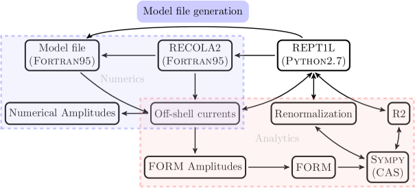
Figure 2: The REPT1L–RECOLA2 tool chain. REPT1L can generate tree-level model files which can then be used in combination with the RECOLA2 library to generate building blocks required in the renormalization process. The process generation is done via the same off-shell currents also used in numerical computations. The currents are evaluated analytically with FORM and further processed with SymPy. The results are then available to REPT1L and are used in the renormalized model file derivation. The red box indicates the analytic computations which uses the tool chain combining RECOLA2, FORM and SymPy. After the renormalized model-file derivation, this tool chain and REPT1L are no longer needed. The blue box, i.e. RECOLA2 and model files, can be used as stand-alone versions (pure Fortran95) for numerical computations.

The renormalization conditions are derived analytically as FORM code. REPT1L uses RECOLA2 to generate the skeletons for processes. The result is written to a FORM file and evaluated, yielding vertex functions which are parsed to Python and processed with SymPy solving the conditions for the counterterm parameters. The procedure is visualized in Fig. 2. Multiple schemes for the very same counterterm parameters can be implemented by imposing different renormalization conditions. All schemes are exported to the RECOLA2 model file and, for a given parameter, a specific scheme can be selected before the process generation phase. For instance, this system can be used to allow the user to choose between different $\mathrm{QCD}$ and $\mathrm{EW}$ renormalization schemes within the same model file. The same system is used for dealing with singularities from light fermions. In general, particles can be tagged as light particles, which, when a particle is subject to on-shell renormalization, makes REPT1L to regularize the associated diagonal two-point function in three different setups, namely dimensional regularization, mass regularization, and keeping the full mass dependence. In a RECOLA2 session a suited regularization scheme for light particles is set automatically, depending on the choice of the mass value, unless the regularization for a particle is explicitly required in a specific scheme. In the case of unstable particles, i.e. massive particles with finite widths, REPT1L applies, by default, the Complex-Mass Scheme (CMS) as discussed in more detail in Section 5.2.

Computation of $R_{2}$ terms

The computation of $R_{2}$ uses the methods developed in Refs. [52, 53, 54] and follows the same computation flow as solving renormalization conditions which is depicted in Fig. 2. For renormalizable theories all existing $R_{2}$ terms can be computed. To this end, REPT1L can generate the skeletons at NLO for all vertex functions in the theory which are potentially UV divergent by power counting. FORM is used to construct each vertex function, replace tensor integrals by their pole parts and take the limit $D\to 4$. The finite parts are identified as Feynman rules associated to the original vertices, which are precisely the $R_{2}$ terms. These steps are done in Python with the help of SymPy.

The computation of tensor coefficients is done in conventional dimensional regularization. Different regularizations will be supported in the future by exchanging the responsible FORM-procedure files. In view of EFTs, the power counting can be disabled, and specific vertex functions can be selected. Further, the $R_{2}$ extraction rules[52, 53, 54] have been extended to higher $n$-point functions and higher rank.

3 HAWK 2.0 interface to RECOLA2

In this section we describe the interface between HAWK 2.0 and RECOLA2 which allows for an automated computation of $\mathrm{NLO}$ $\mathrm{EW}$ and $\mathrm{QCD}$ corrections to observables in associated Higgs production with a vector boson or two jets. We start with the $\mathrm{LO}$ partonic channels and virtual corrections and conclude with the computation of the real corrections. The implementation has been realized in a model-independent way, allowing in the future, apart from the two presented BSM models, for predictions in alternative models.

3.1 Process definitions at $\mathrm{LO}$ and $\mathrm{NLO}$ with RECOLA2

In the case of associated Higgs production with a vector boson, also known as Higgs strahlung, we consider processes with an intermediate vector boson decaying leptonically as

$$\mathrm{p}\mathrm{p}\to\mathrm{H}\mathrm{V}\to\mathrm{H}l^{+}l^{-}/\mathrm{H}l^{\pm}\nu/\mathrm{H}\nu\nu.$$ (3.1)

Depending on the initial-state partons, the intermediate vector boson can be a $\mathrm{Z}$ or a $\mathrm{W}$ boson. For example for the signature $\mathrm{p}\mathrm{p}\to\mathrm{H}\mathrm{Z}\to\mathrm{H}l^{+}l^{-}$, neglecting bottom contributions in the PDFs, there are four different initial-state parton combinations:

$$\bar{}\mathrm{u}\mathrm{u},\quad\bar{}\mathrm{d}\mathrm{d},\quad\bar{}\mathrm{c}\mathrm{c},\quad\bar{}\mathrm{s}\mathrm{s}.$$ (3.2)

Whenever possible, we optimize computations involving different quark generations. For instance, in (3.2) the processes involving the second generation are not computed explicitly, but the results for the first generation are employed instead. For the first generation of quarks the RECOLA2 library is used to generate the processes at tree and one-loop level.

The second process class under consideration is Higgs production in association with two hard jets

$$\mathrm{p}\mathrm{p}\to\mathrm{H}\mathrm{j}\mathrm{j},$$ (3.3)

also known as VBF. There are plenty of partonic channels and, again, we exploit optimizations with respect to the different quark generations. For the $\mathrm{LO}$, virtual $\mathrm{NLO}$ $\mathrm{EW}$, virtual $\mathrm{NLO}$ $\mathrm{QCD}$, real emission $\mathrm{EW}$, and real emission $\mathrm{QCD}$ contributions RECOLA2 generates 32 partonic channels each, with the real kinematic channels corresponding to the Born kinematic ones, with an additional gluon or photon. For the gluon- and photon-induced channels RECOLA2 generates 20 channels each.

At the stage of the process definition the Higgs boson entering in (3.1) or (3.3) can be chosen freely as long as it is supported by the RECOLA2 model file currently in use. For instance, in the case of the 2HDM the Higgs flavour can be set to $H_{\mathrm{l}}$, $H_{\mathrm{h}}$ or $H_{\mathrm{a}}$ (see Section 4), which is done in the HAWK 2.0 input file. In HAWK 2.0 the relevant parameters for process generation and computation are set by input files. This information is forwarded to RECOLA2, allowing to choose specific contributions. The selection works for individual corrections such as $\mathrm{QCD}$ or $\mathrm{EW}$ either virtual or real. For the results presented in this work we selected the pure electroweak corrections, including photon-induced corrections.

3.2 Infrared divergences

RECOLA2 provides the amplitudes for the partonic processes under consideration as well as the colour-correlated squared matrix elements needed for the Catani–Seymour dipole subtraction. In order to deal with IR singularities, an IR subtraction scheme needs to be employed. We adhere to the Catani–Seymour dipole subtraction [55] which is used in HAWK 2.0 and employ mass regularization for soft and collinear divergences, i.e. a small photon mass and small fermion masses are used wherever needed. From the point of view of the interface, dealing with $\mathrm{EW}$ dipoles is a matter of replacing certain Born amplitudes with the ones computed by RECOLA2. As for the $\mathrm{QCD}$ dipoles one needs in general colour-correlated matrix elements. For processes with only two partons, as it is the case for Higgs strahlung, the colour correlation is diagonal owing to colour conservation (see Eq. A1 in Ref. [55]) and again no colour-correlated matrix elements are required. For VBF we compute the colour-correlated matrix elements directly with RECOLA2, and use colour conservation to minimize the number of required computations. The dipoles are used as implemented in HAWK 2.0 and are not part of RECOLA2. For the $\mathrm{QCD}$ dipoles consider Refs. [55, 56] and for $\mathrm{EW}$ dipoles see Refs. [57, 58].

4 2HDM and HSESM model description

In this section, we sketch the definition of the scalar potential of the 2HDM and the HSESM. In both cases we restrict ourselves to a CP-conserving $Z_{2}$-symmetric scalar potential, which in the case of the 2HDM is allowed to be softly broken. For a comprehensive introduction to the 2HDM we refer to Refs. [59, 60] and for the HSESM to the original literature [61, 62, 63] and applications to LHC phenomenology in Refs. [64, 65, 66, 67]. For the kinetic terms we refer to the conventions used in Ref. [64].

4.1 Fields and potential definition

Both models are simple extensions of the SM, only affecting the form and fields entering the scalar potential and for the 2HDM also the Yukawa interactions. In the case of the 2HDM we have two Higgs doublets, generically denoted as $\Phi_{i}$ with $i=1,2$ and defined component-wise by

$$\Phi_{i}=\left(\begin{array}[]{c}\phi_{i}^{+}\\ \frac{1}{\sqrt{2}}\left(v_{i}+\rho_{i}+\mathrm{i}\eta_{i}\right)\end{array}\right),$$ (4.3)

with $v_{i}$ denoting the vevs. Under the constraint of CP conservation plus the $Z_{2}$ symmetry ($\Phi_{1}\to-\Phi_{1},\Phi_{2}\to\Phi_{2}$), the most general, renormalizable potential reads [59]

$$V_{\mathrm{2HDM}}={} m_{1}^{2}\Phi_{1}^{\dagger}\Phi_{1}+m_{2}^{2}\Phi_{2}^{\dagger}\Phi_{2}-m_{12}^{2}\left(\Phi_{1}^{\dagger}\Phi_{2}+\Phi_{2}^{\dagger}\Phi_{1}\right)$$

$$+\frac{\lambda_{1}}{2}\left(\Phi_{1}^{\dagger}\Phi_{1}\right)^{2}+\frac{\lambda_{2}}{2}\left(\Phi_{2}^{\dagger}\Phi_{2}\right)^{2}+\lambda_{3}\left(\Phi_{1}^{\dagger}\Phi_{1}\right)\left(\Phi_{2}^{\dagger}\Phi_{2}\right)+\lambda_{4}\left(\Phi_{1}^{\dagger}\Phi_{2}\right)\left(\Phi_{2}^{\dagger}\Phi_{1}\right)$$

$$+\frac{\lambda_{5}}{2}\left[\left(\Phi_{1}^{\dagger}\Phi_{2}\right)^{2}+\left(\Phi_{2}^{\dagger}\Phi_{1}\right)^{2}\right],$$ (4.4)

with five real couplings $\lambda_{1}\ldots\lambda_{5}$, two real mass parameters $m^{2}_{1}$ and $m^{2}_{2}$, and the soft $Z_{2}$-breaking parameter $m^{2}_{12}$.

The HSESM scalar potential involves one Higgs doublet $\Phi$ and a singlet field $S$ defined as

$$\Phi=\left(\begin{array}[]{c}\phi^{+}\\ \frac{1}{\sqrt{2}}\left(v+\rho_{1}+\mathrm{i}\eta\right)\end{array}\right),\qquad S=\frac{v_{s}+\rho_{2}}{\sqrt{2}}.$$ (4.7)

Under the same constraints, the most general, renormalizable potential reads

$$V_{\mathrm{HSESM}}=m_{1}^{2}\Phi^{\dagger}\Phi+m_{2}^{2}S^{2}+\frac{\lambda_{1}}{2}\left(\Phi^{\dagger}\Phi\right)^{2}+\frac{\lambda_{2}}{2}S^{4}+\lambda_{3}\Phi^{\dagger}\Phi S^{2},$$ (4.8)

with all parameters being real.

4.2 Parameters in the physical basis

Both potentials are subject to spontaneous symmetry breaking which requires a rotation of fields to the mass eigenstates in order to identify the physical degrees of freedom. For the 2HDM there are five physical Higgs bosons $H_{\mathrm{l}},H_{\mathrm{h}},H_{\mathrm{a}},H^{\pm}$ and in the HSESM there are two neutral Higgs bosons $H_{\mathrm{l}}$ and $H_{\mathrm{h}}$, intentionally identified with the same symbols as in the 2HDM. Besides the physical Higgs bosons, there are the three would-be Goldstone bosons $G_{0}$ and $G^{\pm}$ in the ’t Hooft–Feynman gauge. The mass eigenstates for the neutral Higgs-boson fields are obtained in both models by the transformation

$$\left(\begin{array}[]{c}\rho_{1}\\ \rho_{2}\end{array}\right)=R(\alpha)\left(\begin{array}[]{c}H_{\mathrm{h}}\\ H_{\mathrm{l}}\end{array}\right),\quad\text{with}\quad R(\alpha)=\left(\begin{array}[]{cc}\cos\alpha&-\sin\alpha\\ \sin\alpha&\phantom{-}\cos\alpha\end{array}\right),$$ (4.15)

and $\alpha$ being fixed such that the mass matrix

$$M_{ij}:=\left.\frac{\partial^{2}V}{\partial\rho_{i}\partial\rho_{j}}\right|_{\varphi=0},$$ (4.16)

is diagonalized via $R(-\alpha)MR(\alpha)$, with the potential $V$ being either (4.4) or (4.8). The solution to (4.16) for symmetric $2\times 2$ matrices is generically given by (see Ref. [59])

$$\sin 2\alpha=\frac{2M_{12}}{\sqrt{({M}_{11}-M_{22})^{2}+4M_{12}^{2}}}.$$ (4.17)

In the 2HDM there are additional mixings between charged and pseudo-scalar bosons and Goldstone bosons, which are diagonalized as follows

$$\left(\begin{array}[]{c}\phi_{1}^{\pm}\\ \phi_{2}^{\pm}\end{array}\right)={} R(\beta)\left(\begin{array}[]{c}G^{\pm}\\ H^{\pm}\end{array}\right),\qquad\left(\begin{array}[]{c}\eta_{1}\\ \eta_{2}\end{array}\right)=R(\beta)\left(\begin{array}[]{c}G_{0}\\ H_{\mathrm{a}}\end{array}\right),\quad\text{with}\quad R(\beta)=\left(\begin{array}[]{cc}\cos\beta&-\sin\beta\\ \sin\beta&\phantom{-}\cos\beta\end{array}\right).$$ (4.28)

The angle $\beta$ is related to the vevs according to $t_{\beta}\equiv\tan\beta=v_{2}/v_{1}$ in the 2HDM. For the HSESM we define $t_{\beta}\equiv\tan\beta=v_{s}/v$. The Higgs sector is minimally coupled to the gauge bosons. Collecting quadratic terms and identifying the masses one obtains the well-known tree-level relations

$$M_{\mathrm{W}}=\frac{1}{2}gv,\qquad M_{\mathrm{Z}}=\frac{1}{2}\sqrt{g^{2}+{g^{\prime}}^{2}}\;v,\qquad$$ (4.29)

where $g$ and ${g^{\prime}}$ denote the weak isospin and hypercharge gauge couplings, and $M_{\mathrm{W}}$ and $M_{\mathrm{Z}}$ the $\mathrm{W}$- and $\mathrm{Z}$-boson masses, respectively. For the 2HDM we identify $v=\sqrt{v_{1}^{2}+v_{2}^{2}}$. Finally one employs the minimum conditions for the scalar potential which, in both models, read

$$\langle\rho_{i}\rangle=0.$$ (4.30)

Then, one substitutes the potential parameters with physical parameters obtained after spontaneous symmetry breaking and after diagonalizing the Higgs sector. For the 2HDM we choose the Higgs-boson masses $M_{H_{\mathrm{l}}}$ (light Higgs boson), $M_{H_{\mathrm{h}}}$ (heavy Higgs boson), $M_{H_{\mathrm{a}}}$ (pseudoscalar Higgs boson), $M_{H^{\pm}}$ (charged Higgs boson), the soft-$Z_{2}$-breaking scale $M_{\rm sb}$ defined via

$$M_{\rm sb}^{2}=\frac{m_{12}^{2}}{\cos\beta\sin\beta},$$ (4.31)

and the two mixing angles as $c_{\alpha\beta}:=\cos(\alpha-\beta)$ ($s_{\alpha\beta}:=\sin(\alpha-\beta)$) and $t_{\beta}:=\tan(\beta)$, which is a natural choice for studying (almost) aligned scenarios. For the HSESM we use the neutral Higgs-boson masses $M_{H_{\mathrm{l}}}$ (light Higgs boson), $M_{H_{\mathrm{h}}}$ (heavy Higgs boson) and the angles $s_{\alpha}:=\sin(\alpha)$ and $t_{\beta}:=\tan(\beta)$. To summarize, we transform the parameters from the generic basis to the physical one by choosing the following parameters as external ones

2HDM:

$\lambda_{1},\lambda_{2},\lambda_{3},\lambda_{4},\lambda_{5},m_{1},m_{2},m_{12}\;\to\;M_{H_{\mathrm{l}}},M_{H_{\mathrm{h}}},M_{H_{\mathrm{a}}},M_{H^{\pm}},M_{\rm sb},c_{\alpha\beta},t_{\beta},v\left(g,M_{\mathrm{W}}\right),$

HSESM:

$\lambda_{1},\lambda_{2},\lambda_{3},m_{1},m_{2}\;\to\;M_{H_{\mathrm{l}}},M_{H_{\mathrm{h}}},s_{\alpha},t_{\beta},v\left(g,M_{\mathrm{W}}\right),$

where we have indicated that the vev is traded for gauge couplings and masses according to (4.29).

4.3 Yukawa interactions

The fermionic sector in the HSESM is the same as in the SM, whereas the 2HDM allows for a richer structure. In the general case of the 2HDM, fermions can couple to both $\Phi_{1}$ and $\Phi_{2}$, leading to flavour-changing neutral currents (FCNC) already at tree level. Since FCNC processes are extremely rare in nature they highly constrain BSM models. In order to prevent tree-level FCNC, one imposes the $Z_{2}$ symmetry

$$Z_{2}:\quad\Phi_{1}\to-\Phi_{1},\quad\Phi_{2}\to\Phi_{2},$$ (4.32)

as already introduced in the Higgs potential in Section 4.2. This $Z_{2}$ symmetry is motivated by the Glashow–Weinberg–Paschos theorem in Refs. [68, 69], which states that for an arbitrary number of Higgs doublets, if all right-handed fermions couple to exactly one of the Higgs doublets, FCNCs are absent at tree level. This can be realized by imposing, in addition to (4.32), a parity for right-handed fermions under $Z_{2}$ symmetry. One obtains four distinct 2HDM Yukawa terms, the so-called natural flavour-conserving models canonically described in the literature.

Type I:

By requiring for all fermions an even parity under $Z_{2}$, all have to couple to the second Higgs doublet $\Phi_{2}$. The corresponding Yukawa Lagrangian reads

$$\mathcal{L}_{\mathrm{Y}} =-\Gamma_{\mathrm{d}}\overline{Q}_{\mathrm{L}}\Phi_{2}d_{\mathrm{R}}-\Gamma_{\mathrm{u}}\overline{Q}_{\mathrm{L}}\tilde{\Phi}_{2}u_{\mathrm{R}}-\Gamma_{\mathrm{l}}\overline{L}_{\mathrm{L}}\Phi_{2}l_{\mathrm{R}}+\mathrm{h.c.},$$ (4.33)

where $\tilde{\Phi}_{2}$ is the charge-conjugated Higgs doublet of $\Phi_{2}$. Neglecting flavour mixing, the coefficients are directly expressed by the fermion masses $m_{\mathrm{d}}$, $m_{\mathrm{u}}$ and $m_{\mathrm{l}}$, and the mixing angle $\beta$,

$$\Gamma_{\mathrm{d}}=\frac{g\,m_{\mathrm{d}}}{\sqrt{2}M_{\mathrm{W}}\sin\beta},\qquad\Gamma_{\mathrm{u}}=\frac{g\,m_{\mathrm{u}}}{\sqrt{2}M_{\mathrm{W}}\sin\beta},\qquad\Gamma_{\mathrm{l}}=\frac{g\,m_{\mathrm{l}}}{\sqrt{2}M_{\mathrm{W}}\sin\beta}.$$ (4.34)

Again, the vev $v$ has been substituted using Eq. (4.29).

Type II:

This is the MSSM-like scenario obtained by requiring odd parity for down-type quarks and leptons: $d_{\mathrm{R}}\to-d_{\mathrm{R}}$, $l_{\mathrm{R}}\to-l_{\mathrm{R}}$ and even parity for up-type quarks. It follows that the down-type quarks and leptons couple to $\Phi_{1}$, while up-type quarks couple to $\Phi_{2}$. The corresponding Yukawa Lagrangian reads

$$\mathcal{L}_{\mathrm{Y}} =-\Gamma_{\mathrm{d}}\overline{Q}_{\mathrm{L}}\Phi_{1}d_{\mathrm{R}}-\Gamma_{\mathrm{u}}\overline{Q}_{\mathrm{L}}\tilde{\Phi}_{2}u_{\mathrm{R}}-\Gamma_{\mathrm{l}}\overline{L}_{\mathrm{L}}\Phi_{1}l_{\mathrm{R}}+\mathrm{h.c.}.$$ (4.35)

Neglecting flavour mixing, the coefficients are expressed by the fermion masses $m_{\mathrm{d}}$, $m_{\mathrm{u}}$ and $m_{\mathrm{l}}$, and the mixing angle $\beta$,

$$\Gamma_{\mathrm{d}}=\frac{g\,m_{\mathrm{d}}}{\sqrt{2}M_{\mathrm{W}}\cos\beta},\qquad\Gamma_{\mathrm{u}}=\frac{g\,m_{\mathrm{u}}}{\sqrt{2}M_{\mathrm{W}}\sin\beta},\qquad\Gamma_{\mathrm{l}}=\frac{g\,m_{\mathrm{l}}}{\sqrt{2}M_{\mathrm{W}}\cos\beta}.$$ (4.36)

Type Y:

This type, also referred to as lepton-specific 2HDM, is obtained by requiring odd parity only for leptons: $l_{\mathrm{R}}\to-l_{\mathrm{R}}$.

Type X:

This type, also referred to as flipped 2HDM, is obtained by requiring odd parity only for down-type quarks: $d_{\mathrm{R}}\to-d_{\mathrm{R}}$.

In the analysis of this paper we focus on Type II, which is equivalent to Type I for massless leptons and quarks, except for the top quark. We remark that exactly one RECOLA2 model file can handle all Yukawa types, and switching between different Yukawa types is done by a simple function call.

5 Background-Field Method for extended Higgs sectors

The BFM is a powerful formulation for gauge theories which renders analytic calculations easier due to a simple structure of the Feynman rules and additional symmetry relations. The method was originally derived by DeWitt in Refs. [70, 71] and has since then been used in many applications. The additional symmetry relations emerge for gauge theories in combination with a suited gauge-fixing term and encode the invariance of the theory under so-called Background-Field gauge invariance. This property is particularly useful for the calculations of $\beta$ functions [73] in higher orders and is also of interest in beyond flat space-time quantum field theory. The BFM can be used to calculate $S$-matrix elements, as constructed in Ref. [74], which, despite having to deal with many more Feynman rules, is in our implementation as efficient as the conventional formalism. Further, the BFM, which can be viewed as a different choice of gauge, allows for an alternative way of computing $S$-matrix elements and, thus, provides a powerful check of the consistency of the REPT1L/RECOLA2 tool chain. This is particularly useful for the validation of $R_{2}$ terms where mistakes are difficult to spot. In addition, we checked a few Background-Field Ward identities. We stress that the BFM can be used as a complementary method in RECOLA2 besides the usual formulation. Even though the use of the BFM in practical calculations is steered in precisely the same way as for model files in the conventional formulation, the internal machinery is different. In particular, the derivation of the Feynman rules and renormalization procedure requires special attention which is discussed in the following.

5.1 BFM action for extended Higgs sector

The results presented here are a simple generalization of Ref. [75], which deals with the BFM applied to the SM at one-loop order. The BFM splits fields in background and quantum fields and combines the new action with a special choice for the gauge-fixing function resulting in a manifest background-field gauge invariance for the effective action at the quantum level. This splitting separates the classical solutions of the field equations, represented by background fields, from the quantum excitation modes, represented by quantum fields. The Feynman rules are derived as usual, treating background and quantum fields on equal footing, which we have done with Feynrules. In principle, the splitting can be done for every field in the theory, however, as we are only interested in a background-field gauge-invariant action, it is sufficient to shift fields which enter the gauge-fixing function. Thus, we perform

$${W}^{a,\mu}\to\underline{W}^{a,\mu}:={W}^{a,\mu}+\hat{W}^{a,\mu},\qquad B^{\mu}\to\underline{B}^{\mu}:=B^{\mu}+\hat{B}^{\mu},$$

$$\Phi_{i}\to\underline{\Phi}_{i}:=\Phi_{i}+\hat{\Phi}_{i},\qquad\qquad S\to\underline{S}:=S+\hat{S},$$ (5.1)

where $W^{a}$ $(\hat{W}^{a})$ and $B$ $(\hat{B})$ are the SM quantum (background) gauge fields in the gauge eigenbasis with $a=1,2,3$. The index $i$ runs over all Higgs doublets $\Phi_{i}$ in the theory under consideration, and $S$ is a singlet field, absent in the 2HDM or SM. While the singlet field $S$ does not appear explicitly in the gauge-fixing function [see (5.7)], the inclusion of $S$ in the splitting (5.1) is necessary due to the mixing with the neutral component of a Higgs doublet. The components for the background- and quantum-field doublets are defined as

$$\Phi_{i}=\left(\begin{array}[]{c}\phi_{i}^{+}\\ \frac{1}{\sqrt{2}}\left(\rho_{i}+\mathrm{i}\eta_{i}\right)\end{array}\right),\qquad\hat{\Phi}_{i}=\left(\begin{array}[]{c}\hat{\phi}_{i}^{+}\\ \frac{1}{\sqrt{2}}\left(v_{i}+\hat{\rho}_{i}+\mathrm{i}\hat{\eta}_{i}\right)\end{array}\right).$$ (5.6)

By convention, we keep the original vev of the Higgs doublet in the Higgs background-field doublet. The quantum gauge-fixing term has the traditional form. In the gauge eigenbasis it reads

$$\mathcal{L}_{\mathrm{GF}}=-\frac{1}{2}\sum_{a=1}^{3}\left(F_{W}^{a}\right)^{2}-\frac{1}{2}F_{B}^{2},$$ (5.7)

with generalized gauge-fixing functions

$$F_{W}^{a} =\hat{D}^{\mu}{W}^{a}_{\mu}-\mathrm{i}\frac{g}{2}\sum_{i}\left[\hat{\Phi}_{i}^{\dagger}\sigma^{a}\Phi_{i}-\Phi_{i}^{\dagger}\sigma^{a}\hat{\Phi}_{i}\right],$$

$$F_{B} =\partial^{\mu}B_{\mu}+\mathrm{i}\frac{{g^{\prime}}}{2}\sum_{i}\left[\hat{\Phi}_{i}^{\dagger}\Phi_{i}-\Phi_{i}^{\dagger}\hat{\Phi}_{i}\right],$$ (5.8)

and $i$ running over all Higgs doublets. The covariant derivative $\hat{D}$ is similar to the usual one, but with a background-field gauge connection instead of a quantum-field one. For a field $\alpha^{j}$ in the adjoint representation it acts in the following way

$$\hat{D}_{\mu}\alpha^{a}=\partial_{\mu}\alpha^{a}+g\epsilon^{abc}\hat{W}^{b}_{\mu}\alpha^{c},$$ (5.9)

with $\epsilon^{abc}$ being the structure constants of SU(2). The form (5.7), (5.8) is invariant under background-field gauge transformations, which can be shown using the techniques presented in Ref. [72], but suitably generalized in the presence of spontaneous symmetry breaking.

The construction of the ghost term follows the standard BRST quantization procedure. Once the symmetry transformations are defined on the fields, a valid ghost Lagrangian, leading to a BRST invariant action, is given by

$$\mathcal{L}_{\mathrm{ghost}}=-\sum_{a=1}^{3}\bar{u}_{W}^{a}\delta_{\mathrm{B}}{F}_{W}^{a}-\bar{u}_{B}\delta_{\mathrm{B}}F_{B}.$$ (5.10)

The fields in the gauge eigenbasis are rotated to the physical basis in the following way

$$W_{\mu}^{1}=\frac{W_{\mu}^{-}+W_{\mu}^{+}}{\sqrt{2}},\quad W_{\mu}^{2}=\frac{W_{\mu}^{-}-W_{\mu}^{+}}{\mathrm{i}\sqrt{2}},\quad W_{\mu}^{3}=c_{\mathrm{w}}Z_{\mu}-s_{\mathrm{w}}A_{\mu},\quad B_{\mu}=s_{\mathrm{w}}Z_{\mu}+c_{\mathrm{w}}A_{\mu},$$

$$u_{W}^{1}=\frac{u_{W}^{-}+u_{W}^{+}}{\sqrt{2}},\quad u_{W}^{2}=\frac{u_{W}^{-}-u_{W}^{+}}{\mathrm{i}\sqrt{2}},\quad u_{W}^{3}=c_{\mathrm{w}}u_{Z}-s_{\mathrm{w}}u_{A},\quad u_{B}=s_{\mathrm{w}}u_{Z}+c_{\mathrm{w}}u_{A}.$$ (5.11)

The BRST transformations on the gauge eigenbasis, expressed in terms of physical fields via (5.11), read

$$\delta_{\mathrm{B}}W^{1}_{\mu}=\underline{D}_{\mu}u_{W}^{1}=$$

$$\frac{1}{\sqrt{2}}\partial_{\mu}\left(u_{W}^{-}+u_{W}^{+}\right)-\frac{\mathrm{i}e}{\sqrt{2}}\left[\left(u_{W}^{-}-u_{W}^{+}\right)\left(\underline{A}_{\mu}-\frac{c_{\mathrm{w}}}{s_{\mathrm{w}}}\underline{Z}_{\mu}\right)+\left(u_{A}-\frac{c_{\mathrm{w}}}{s_{\mathrm{w}}}u_{Z}\right)\left(\underline{W}_{\mu}^{+}-\underline{W}_{\mu}^{-}\right)\right],$$ (5.12)

$$\delta_{\mathrm{B}}W^{2}_{\mu}=\underline{D}_{\mu}u_{W}^{2}=$$

$$\frac{\mathrm{i}}{\sqrt{2}}\partial_{\mu}\left(u_{W}^{+}-u_{W}^{-}\right)-\frac{e}{\sqrt{2}}\left[\left(u_{W}^{-}+u_{W}^{+}\right)\left(\underline{A}_{\mu}-\frac{c_{\mathrm{w}}}{s_{\mathrm{w}}}\underline{Z}_{\mu}\right)-\left(u_{A}-\frac{c_{\mathrm{w}}}{s_{\mathrm{w}}}u_{Z}\right)\left(\underline{W}_{\mu}^{+}+\underline{W}_{\mu}^{-}\right)\right],$$ (5.13)

$$\delta_{\mathrm{B}}W^{3}_{\mu}=\underline{D}_{\mu}u_{W}^{3}=\partial_{\mu}\left(c_{\mathrm{w}}u_{Z}-s_{\mathrm{w}}u_{A}\right)-\frac{\mathrm{i}e}{s_{\mathrm{w}}}\left(u_{W}^{-}\underline{W}^{+}-u_{W}^{+}\underline{W}^{-}\right),$$ (5.14)

$$\delta_{\mathrm{B}}B_{\mu}=\underline{D}_{\mu}u_{B}=\partial_{\mu}\left(c_{\mathrm{w}}u_{A}+s_{\mathrm{w}}u_{Z}\right).$$ (5.15)

Note that in contrast to the conventional formalism, the covariant derivatives entering the BRST transformations use the shifted gauge fields (5.1). For the Higgs doublets the BRST transformation rules can be defined at the level of components as follows

$$\delta_{\mathrm{B}}\Phi_{i}:=\left(\begin{array}[]{c}\delta_{\mathrm{B}}\phi_{i}^{+}\\ \frac{1}{\sqrt{2}}\left(\delta_{\mathrm{B}}\rho_{i}+\mathrm{i}\delta_{\mathrm{B}}\eta_{i}\right)\end{array}\right),$$ (5.18)

with

$$\delta_{\mathrm{B}}\phi_{i}^{+} =\frac{\mathrm{i}e}{2s_{\mathrm{w}}}(\mathrm{i}\underline{\eta}_{i}+\underline{\rho}_{i}+v_{i})u_{W}^{+}+\frac{\mathrm{i}e\left(c_{\mathrm{w}}^{2}-s_{\mathrm{w}}^{2}\right)}{2c_{\mathrm{w}}s_{\mathrm{w}}}\underline{\phi}_{i}^{+}u_{Z}-\mathrm{i}e\underline{\phi}_{i}^{+}u_{A}$$ (5.19)

$$\delta_{\mathrm{B}}\rho_{i} =\frac{e}{2c_{\mathrm{w}}s_{\mathrm{w}}}\underline{\eta}_{i}u_{Z}+\frac{\mathrm{i}e}{2s_{\mathrm{w}}}\left(\underline{\phi}_{i}^{+}u_{W}^{-}-\underline{\phi}_{i}^{-}u_{W}^{+}\right)$$ (5.20)

$$\delta_{\mathrm{B}}\eta_{i} =-\frac{e}{2c_{\mathrm{w}}s_{\mathrm{w}}}\left(\underline{\rho}_{i}+v_{i}\right)u_{Z}+\frac{e}{2s_{\mathrm{w}}}\left(\underline{\phi}_{i}^{+}u_{W}^{-}+\underline{\phi}_{i}^{-}u_{W}^{+}\right)$$ (5.21)

The transformations for $\delta_{\mathrm{B}}\rho_{i}$ and $\delta_{\mathrm{B}}\eta_{i}$ are fixed by taking the real and imaginary part of the BRST transformation of the lower doublet component, respectively. In this way, if the ghost term is formulated directly in the physical basis, as it is done in Ref. [75], the Lagrangian is guaranteed to be hermitian.

5.2 Renormalization in the BFM

The renormalization in the BFM is performed in the same fashion as in the conventional formulation, except that only background fields need to be renormalized. REPT1L can distinguish between both types of fields by checking the field-type attribute. A field can be assigned to be a background and/or quantum field. In the conventional formalism, all fields play both roles and can thus appear in tree and loop amplitudes. In the presence of pure quantum fields, as it is the case in the BFM, the only contributing Feynman rules to tree and one-loop amplitudes are the ones with exactly none or two quantum fields.

Since we aim at the computation of $S$-matrix elements, an on-shell renormalization of physical fields is suited. However, fixing the field renormalization constants via on-shell conditions breaks background-field gauge invariance and, as a consequence, some Ward identities are not fulfilled. The reason is that demanding background-field gauge invariance requires, in particular, a uniform renormalization of all covariant derivatives in the theory which is only possible if the field renormalization constants of gauge fields are not independent parameters but chosen accordingly [75]. Since the theory is governed by BRST invariance, the breaking of the background-field Ward identities does not pose a problem, especially not for the renormalizability of the theory and the gauge independence of observables. Yet, we do not break the QED background-field Ward identity, which relates the fermion–fermion–photon vertex to fermionic self-energies [75]

$$k_{\mu}\Gamma_{\mu}^{\gamma\bar{f}f}(k,p,p^{\prime})=-eQ_{f}\left[\Gamma^{\bar{f}f}\left(p\right)-\Gamma^{\bar{f}f}\left(p^{\prime}\right)\right],$$ (5.22)

and can be used to fix the photon field renormalization constant or the counterterm $\delta Z_{e}$. Requiring (5.22) for renormalized vertex functions yields the well-known one-loop relation in the BFM

$$\delta Z_{e}=-\frac{\delta Z_{A}}{2},$$ (5.23)

which is consistent with the renormalization of $\alpha$ in the TL and the photon renormalized on-shell. For LHC phenomenology the TL does not provide an appropriate renormalization due to the difference of the scale in the underlying processes. A popular choice is the $G_{\mathrm{F}}$ scheme [76, 77, 78] which can be defined via the muon decay. To this end, the renormalized electric charge is related to the experimentally measured value for the Fermi constant $G_{\mathrm{F}}$. At one-loop order, neglecting pure QED corrections, finite corrections to the renormalization in the TL are defined by $\Delta r$

$$\delta Z_{e}^{G_{\mathrm{F}}}=\delta Z_{e}^{\mathrm{TL}}-\frac{\Delta r}{2},$$ (5.24)

where in the SM [51]

$$\Delta r =\frac{\Sigma_{WW}^{\mathrm{1PI},\mathrm{T}}\left(0\right)-\Sigma_{WW}^{\mathrm{1PI},\mathrm{T}}\left(\mu_{\mathrm{W}}^{2}\right)}{\mu_{\mathrm{W}}^{2}}+\frac{2}{c_{\mathrm{w}}s_{\mathrm{w}}}\frac{\Sigma_{AZ}^{\mathrm{1PI},\mathrm{T}}(0)}{\mu_{\mathrm{Z}}^{2}}+\frac{2\delta g}{g}$$

$$+\frac{g^{2}}{16\pi^{2}}\left[\frac{\log\left(c_{\mathrm{w}}^{2}\right)}{s_{\mathrm{w}}^{2}}\left(\frac{7}{2}-2s_{\mathrm{w}}^{2}\right)+6\right],$$ (5.25)

and $\Sigma^{\mathrm{1PI},\mathrm{T}}$ being an unrenormalized transverse 1PI mixing or self-energy. Note that all terms, except for the $\mathrm{W}$ self-energy, originate from vertex and box corrections, in particular, the term $\Sigma_{AZ}^{\mathrm{1PI},\mathrm{T}}$ has just been introduced to match the divergence structure. Equation (5.25) is valid for the conventional formulation in the ’t Hooft–Feynman gauge, but not in the BFM since mixing and self-energies, or, in general, vertex functions differ by gauge-dependent terms in both formulations. Since the parameter $\Delta r$ connects physical quantities it is necessarily gauge independent, which implies that both formulations differ merely by a reshuffling of gauge-dependent terms between the self-energy and vertex parts. We have determined the difference in the vertex corrections between the BFM and conventional formulation in the ’t Hooft–Feynman gauge, and, as expected, it cancels against the difference in the $\mathrm{W}$ self-energy. For a model-independent evaluation in the BFM, the result can be expressed in the same form as (5.25), but with a modified vertex correction

$$\Delta r =\frac{\Sigma_{WW}^{\mathrm{1PI},\mathrm{BFM},\mathrm{T}}(0)-\Sigma_{WW}^{\mathrm{1PI},\mathrm{BFM},\mathrm{T}}\left(\mu_{\mathrm{W}}^{2}\right)}{\mu_{\mathrm{W}}^{2}}+\frac{2}{c_{\mathrm{w}}s_{\mathrm{w}}}\frac{\Sigma_{AZ}^{\mathrm{1PI},\mathrm{BFM},\mathrm{T}}(0)}{\mu_{\mathrm{Z}}^{2}}+\frac{2\delta g}{g}$$

$$+\frac{g^{2}}{16\pi^{2}}\left[\frac{\log\left(c_{\mathrm{w}}^{2}\right)}{s_{\mathrm{w}}^{2}}\left(-\frac{1}{2}+2s_{\mathrm{w}}^{2}\right)+2\right],$$ (5.26)

which is valid only in the ’t Hooft–Feynman gauge in the BFM.

Another subtlety concerns the renormalization within the CMS. REPT1L automatically renormalizes unstable particles in the CMS following the general prescription of Refs. [79, 80, 81]. The corresponding on-shell renormalization conditions require scalar integrals to be analytically continued to complex squared momenta. This can be avoided by using an expansion around real momentum arguments, which gives rise to gauge-dependent terms of higher perturbative orders. Thus, comparing the BFM to the conventional formalism leads to somewhat different results for finite widths. The effect can be traced back to the difference of full self-energies in both formulations, e.g. the difference in the $\mathrm{W}$ self-energy is given by

$$\Sigma_{WW}^{\mu\nu,\mathrm{BFM}}(p)-\Sigma_{WW}^{\mu\nu}(p)=\frac{g^{2}}{4\pi^{2}}\left(\mu_{\mathrm{W}}^{2}-p^{2}\right)g^{\mu\nu}\left[c_{\mathrm{w}}^{2}B_{0}\left(p^{2},\mu_{\mathrm{Z}},\mu_{\mathrm{W}}\right)+s_{\mathrm{w}}^{2}B_{0}\left(p^{2},0,\mu_{\mathrm{W}}\right)\right],$$ (5.27)

with the conventions for scalar integrals as in Ref. [51]. The gauge dependence drops out in the mass renormalization constant, i.e. ${\delta\mu_{\mathrm{W}}^{2}}^{\mathrm{BFM}}=\delta\mu_{\mathrm{W}}^{2}$ in the CMS, because the self-energy is evaluated on the complex pole, i.e. for $p^{2}=\mu_{\mathrm{W}}^{2}$. However, performing an expansion of the self-energy around the real mass $M_{\mathrm{W}}^{2}$ results in differences of the order of $\mathcal{O}\left(\alpha^{3}\right)$. For a comparison of both formulations it is useful to modify the expanded (exp) mass counterterm to match the conventional formalism in the following way

$${\delta\mu_{\mathrm{W}}^{2}}^{\mathrm{BFM}}_{,\mathrm{exp}} \to{\delta\mu_{\mathrm{W}}^{2}}_{,\mathrm{exp}}=$$

$$={\delta\mu_{\mathrm{W}}^{2}}^{\mathrm{BFM}}_{,\mathrm{exp}}-\frac{g^{2}}{4\pi^{2}}\left(M_{\mathrm{W}}^{2}-\mu_{\mathrm{W}}^{2}\right)^{2}\left[c_{\mathrm{w}}^{2}B_{0}^{\prime}\left(M_{\mathrm{W}}^{2},\mu_{\mathrm{Z}},\mu_{\mathrm{W}}\right)+s_{\mathrm{w}}^{2}B_{0}^{\prime}\left(M_{\mathrm{W}}^{2},0,\mu_{\mathrm{W}}\right)\right],$$ (5.28)

with $B_{0}^{\prime}$ being defined as the derivative of $B_{0}$ with respect to $p^{2}$. Note that the difference is of order $\mathcal{O}(\alpha^{3})$ and phenomenologically irrelevant.

The renormalization of the tadpoles in the BFM is performed analogously to the conventional formulation. From a theoretical point of view the renormalization of tadpoles is not necessary, and the theory is well-defined just by including tadpole graphs everywhere. However, in practical calculations it is desirable to avoid unnecessary computations of graphs with explicit tadpoles if their contribution can be included indirectly by other means, e.g. via a suited renormalization. The renormalization of the tadpoles has to be done with care because a naive treatment of the tadpole counterterms can lead to spurious dependencies on the gauge-fixing procedure which ultimately spoil the gauge independence of the one-loop part of $S$-matrix elements. From the point of view of applicability, automation and gauge independence, we strongly recommend the FJ Tadpole Scheme, which has been automated for arbitrary theories [23]. In contrast to other schemes, the FJ Tadpole Scheme is purely based on the field reparametrization invariance of quantum field theory (see Ref. [23]), which can be shown to be equivalent to not renormalizing the tadpoles at all, but with the benefit of not having to compute graphs with explicit tadpoles. Under the general assumption that the theory under consideration is expressed in the physical basis without tree-level mixings and restricting to the one-loop case, the FJ Tadpole Scheme is equivalent to the field redefinition

$$\hat{H}_{i}\to\hat{H}_{i}-\frac{\delta t_{\hat{H}_{i}}}{m_{\hat{H}_{i}}^{2}},$$ (5.29)

for every physical (background-)field $\hat{H}_{i}$ that develops a vev and with $\delta t_{\hat{H}_{i}}$ being the associated tadpole counterterm. By fixing $\delta t_{\hat{H}_{i}}$ to the tadpole graphs $T_{\hat{H}_{i}}$ via

$$\delta t_{\hat{H}_{i}}=-T_{\hat{H}_{i}},$$ (5.30)

explicit tadpoles are cancelled and only tadpole counterterms to 1PI graphs remain. REPT1L can automatically derive all tadpole counterterms in the FJ Tadpole Scheme. In the FJ Tadpole Scheme the value of each counterterm needs to be independent of $\delta t_{\hat{H}_{i}}$ which can be verified analytically. Additional checks concerning the tadpole renormalization can be performed on a process-by-process basis by including the tadpole graphs explicitly instead of renormalizing them. Finally, we note that RECOLA2 is able to use any tadpole counterterm scheme, but only the FJ Tadpole Scheme is fully automated.

6 Setup and benchmark points

6.1 Input parameters

For the numerical analysis in the two Higgs-boson production processes we use the following values for the SM input parameters [84]:

$$G_{\mathrm{F}}=1.16638\cdot 10^{-5}\,\mathrm{GeV}^{-2},\quad m_{\mathrm{t}}=173.21\,\mathrm{GeV},\quad M_{\mathrm{h}}=125.09\,\mathrm{GeV},$$

$$M_{\mathrm{W}}=80.385\,\mathrm{GeV},\quad\Gamma_{\mathrm{W}}=2.085\,\mathrm{GeV},\quad M_{\mathrm{Z}}=91.1876\,\mathrm{GeV},\quad\Gamma_{\mathrm{Z}}=2.4952\,\mathrm{GeV}.$$ (6.1)

For the 2HDM we present updated and new results for the benchmark points in Tables 1 and 3 as proposed by the HXSWG [85]. The corresponding Higgs self-couplings $\lambda_{i}$ are given for convenience in Tables 2 and 4. For the HSESM we compiled a list of benchmark points in Table 5 featuring different hierarchies and being compatible with the limits given in Refs. [65, 66]. The results include the SM-like and heavy Higgs-boson production for both models. The computations were carried out in the ’t Hooft–Feynman gauge both in the conventional formalism and in the BFM. In case of the 2HDM the matrix elements have undergone additional tests. Most notably, we have compared results obtained with RECOLA2 for Higgs decays into four fermions, which is closely related to the considered processes, to an independent calculation[86] based on FeynArts/FormCalc[7, 8] for various channels. We found agreement to more than 7 digits for 3348 out of 3500 phase-space points in the virtual amplitude, none differing by more than 5 digits. We compared off-shell two-point functions for all distinct external states, i.e. scalars, fermions, and vector bosons, against an independent approach in QGRAF [87] and QGS, which is an extension of GraphShot[88]. Against the same setup we compared Higgs decays into scalars, fermions and vector bosons on amplitude level. In addition, we verified (on-shell) Slavnov–Taylor identities for two-point functions (see Eq. (4.16) and the following in Ref. [86]).

6.2 Cut setup

For the analysis of Higgs strahlung we consider the case of two charged muons in the final state, $\mathrm{p}\mathrm{p}\to\mathrm{H}\mathrm{\mu}^{+}\mathrm{\mu}^{-}+X$. The muons are not recombined with collinear photons, and are assumed to be perfectly isolated, treated as bare muons as described in Ref. [21]. We use the cuts given in Ref. [89], i.e. we demand the muons to

• have transverse momentum $p_{\mathrm{T},l}>20\,\mathrm{GeV}$ for $l=\mathrm{\mu}^{+},\mathrm{\mu}^{-}$,

• be central with rapidity $\left|y_{l}\right|<2.4$ for $l=\mathrm{\mu}^{+},\mathrm{\mu}^{-}$,

• have a pair invariant mass $m_{\mu\mu}$ of $75\,\mathrm{GeV}<m_{\mathrm{\mu}\mathrm{\mu}}<105\,\mathrm{GeV}$.

Further, we select boosted events with a

• transverse momentum $p_{\mathrm{T},\mathrm{\mu}\mathrm{\mu}}>160\,\mathrm{GeV}$.

For VBF we employ the cuts as suggested by the HXSWG in Ref. [85], i.e. we require two hard jets $\mathrm{j}_{i},i=1,2$, emerging from partons $i$ with

• pseudo-rapidity $\left|\eta_{i}\right|<5$.

The recombination is done in the anti-$k_{T}$ algorithm [90] with jet size $D=0.4$. Further, events pass the cuts if the two hard jets have

• a transverse momentum $p_{\mathrm{T},\mathrm{j}_{i}}>19\,\mathrm{GeV}$ each,

• a rapidity $\left|y_{\mathrm{j}_{i}}\right|<5$ each,

• a rapidity difference $\left|y_{\mathrm{j}_{1}}-y_{\mathrm{j}_{2}}\right|>3$,

• an invariant mass $M_{\mathrm{j}_{1}\mathrm{j}_{2}}>130\,\mathrm{GeV}$.

We present the results for hadronic cross sections at the centre-of-mass energy of 13 TeV using the NLO PDF set NNPDF2.3 with QED corrections [91].

	$M_{H_{\mathrm{h}}}$	$M_{H_{\mathrm{a}}}$	$M_{H^{\pm}}$	$m_{12}$	$t_{\beta}$	$M_{\rm sb}$
BP21A	$200\,\mathrm{GeV}$	$500\,\mathrm{GeV}$	$200\,\mathrm{GeV}$	$135\,\mathrm{GeV}$	$1.5$	$198.7\,\mathrm{GeV}$
BP21B	$200\,\mathrm{GeV}$	$500\,\mathrm{GeV}$	$500\,\mathrm{GeV}$	$135\,\mathrm{GeV}$	$1.5$	$198.7\,\mathrm{GeV}$
BP21C	$400\,\mathrm{GeV}$	$225\,\mathrm{GeV}$	$225\,\mathrm{GeV}$	$0\,\mathrm{GeV}$	$1.5$	$0\,\mathrm{GeV}$
BP21D	$400\,\mathrm{GeV}$	$100\,\mathrm{GeV}$	$400\,\mathrm{GeV}$	$0\,\mathrm{GeV}$	$1.5$	$0\,\mathrm{GeV}$
BP3A1	$180\,\mathrm{GeV}$	$420\,\mathrm{GeV}$	$420\,\mathrm{GeV}$	$70.71\,\mathrm{GeV}$	$3$	$129.1\,\mathrm{GeV}$

Table 1: 2HDM benchmark points in the alignment limit, i.e. $s_{\alpha\beta}\to-1$, $c_{\alpha\beta}\to 0$, taken from Ref. [92]. The parameter $M_{\rm sb}$ depends on the other parameters and is given for convenience.

	$\lambda_{1}$	$\lambda_{2}$	$\lambda_{3}$	$\lambda_{4}$	$\lambda_{5}$
BP21A	$0.28$	$0.26$	$0.27$	$3.45$	$-3.47$
BP21B	$0.28$	$0.26$	$7.19$	$-3.47$	$-3.47$
BP21C	$6.19$	$1.43$	$-0.71$	$-0.83$	$-0.83$
BP21D	$6.19$	$1.43$	$2.89$	$-5.11$	$-0.16$
BP3A1	$2.59$	$0.29$	$5.26$	$-2.63$	$-2.63$

Table 2: Higgs self-couplings for the 2HDM benchmark points in the alignment limit. We omit the imaginary parts appearing in the CMS.

	$M_{H_{\mathrm{h}}}$	$M_{H_{\mathrm{a}}}$	$M_{H^{\pm}}$	$m_{12}$	$t_{\beta}$	$c_{\alpha\beta}$	$M_{\rm sb}$
a-1	$700\,\mathrm{GeV}$	$700\,\mathrm{GeV}$	$670\,\mathrm{GeV}$	$424.3\,\mathrm{GeV}$	$1.5$	$-0.0910$	$624.5\,\mathrm{GeV}$
b-1	$200\,\mathrm{GeV}$	$383\,\mathrm{GeV}$	$383\,\mathrm{GeV}$	$100\,\mathrm{GeV}$	$2.52$	$-0.0346$	$204.2\,\mathrm{GeV}$
BP22A	$500\,\mathrm{GeV}$	$500\,\mathrm{GeV}$	$500\,\mathrm{GeV}$	$187.08\,\mathrm{GeV}$	$7$	$0.28$	$500\,\mathrm{GeV}$
BP3B1	$200\,\mathrm{GeV}$	$420\,\mathrm{GeV}$	$420\,\mathrm{GeV}$	$77.78\,\mathrm{GeV}$	$3$	$0.3$	$142.0\,\mathrm{GeV}$
BP3B2	$200\,\mathrm{GeV}$	$420\,\mathrm{GeV}$	$420\,\mathrm{GeV}$	$77.78\,\mathrm{GeV}$	$3$	$0.5$	$142.0\,\mathrm{GeV}$
BP43	$263.7\,\mathrm{GeV}$	$6.3\,\mathrm{GeV}$	$308.3\,\mathrm{GeV}$	$52.32\,\mathrm{GeV}$	$1.9$	$0.14107$	$81.5\,\mathrm{GeV}$
BP44	$227.1\,\mathrm{GeV}$	$24.7\,\mathrm{GeV}$	$226.8\,\mathrm{GeV}$	$58.37\,\mathrm{GeV}$	$1.8$	$0.14107$	$89.6\,\mathrm{GeV}$
BP45	$210.2\,\mathrm{GeV}$	$63.06\,\mathrm{GeV}$	$333.5\,\mathrm{GeV}$	$69.2\,\mathrm{GeV}$	$2.4$	$0.71414$	$116.2\,\mathrm{GeV}$

Table 3: 2HDM benchmark points outside the alignment limit taken from Ref. [93] (a-1, b-1) and Ref. [92]. The parameter $M_{\rm sb}$ depends on the other parameters and is given for convenience.

	$\lambda_{1}$	$\lambda_{2}$	$\lambda_{3}$	$\lambda_{4}$	$\lambda_{5}$
a-1	$1.76$	$1.97$	$0.09$	$-0.29$	$-1.65$
b-1	$0.01$	$0.26$	$3.72$	$-1.73$	$-1.73$
BP22A	$0.26$	$0.26$	$7.98$	$0.$	$0.$
BP3B1	$3.60$	$0.25$	$5.46$	$-2.57$	$-2.57$
BP3B2	$3.44$	$0.27$	$5.74$	$-2.57$	$-2.57$
BP43	$4.42$	$0.43$	$2.34$	$-3.02$	$0.11$
BP44	$2.85$	$0.40$	$1.10$	$-1.55$	$0.12$
BP45	$3.16$	$0.35$	$3.92$	$-3.38$	$0.16$

Table 4: Higgs self-couplings for the 2HDM benchmark points outside the alignment limit. We omit the imaginary parts appearing in the CMS.

	$M_{H_{\mathrm{h}}}/\,\mathrm{GeV}$	$t_{\beta}$	$s_{\alpha}$	$\lambda_{1}$	$\lambda_{2}$	$\lambda_{3}$
BP1	$500$	$2.2$	$-0.979796$	$0.41$	$0.82$	$-0.34$
BP2	$400$	$1.7$	$-0.96286$	$0.43$	$0.85$	$-0.36$
BP3	$300$	$1.3$	$-0.950737$	$0.38$	$0.81$	$-0.28$
BP4	$200$	$0.85$	$-0.932952$	$0.31$	$0.84$	$-0.16$
	$M_{H_{\mathrm{l}}}/\,\mathrm{GeV}$	$t_{\beta}$	$s_{\alpha}$	$\lambda_{1}$	$\lambda_{2}$	$\lambda_{3}$
BP5	$100$	$0.35$	$-0.35$	$0.25$	$1.44$	$-0.09$
BP6	$50$	$0.2$	$-0.06$	$0.26$	$1.05$	$-0.06$

Table 5: HSESM benchmark points compiled from Ref. [94]. In the upper table typical scenarios are depicted with a heavy additional scalar Higgs boson. In the lower table inverted scenarios are listed with $H_{\mathrm{h}}$ identified as the SM Higgs boson and mass $M_{H_{\mathrm{h}}}=125.09\,\mathrm{GeV}$. The Higgs self-couplings $\lambda_{i}$ depend on the other parameters and their real parts are given for convenience.

6.3 Mixing angles at one-loop order

The prime vertices of interest in the processes studied in Section 7 are the $H_{\mathrm{l}}\mathrm{V}\mathrm{V}$ and $H_{\mathrm{h}}\mathrm{V}\mathrm{V}$ vertices. Thus, the relevant one-loop corrections require to renormalize $\alpha$ and $\beta$ in the 2HDM and $\alpha$, but not $\beta$, in the HSESM. We present the counterterms for the mixing angles in an ${\overline{\mathrm{MS}}}$ scheme and two different on-shell schemes in the following:

${\overline{\mathrm{MS}}}$:

The mixing angles $\alpha$, $\beta$ are renormalized using ${\overline{\mathrm{MS}}}$ subtraction[23] for the vertices $H_{\mathrm{l}}\to\tau^{+}\tau^{-}$, $H_{\mathrm{a}}\to\tau^{+}\tau^{-}$, respectively, with $\beta$ only being renormalized in the 2HDM. This is equivalent to using the identities

$$\delta\alpha =\frac{\delta Z_{H_{\mathrm{h}}H_{\mathrm{l}}}^{{\overline{\mathrm{MS}}}}-\delta Z_{H_{\mathrm{l}}H_{\mathrm{h}}}^{{\overline{\mathrm{MS}}}}}{4}=\frac{\Sigma^{\mathrm{1PI},{\overline{\mathrm{MS}}}}_{H_{\mathrm{h}}H_{\mathrm{l}}}\left(M_{H_{\mathrm{h}}}^{2}\right)+\Sigma^{\mathrm{1PI},{\overline{\mathrm{MS}}}}_{H_{\mathrm{h}}H_{\mathrm{l}}}\left(M_{H_{\mathrm{l}}}^{2}\right)+2t_{H_{\mathrm{l}}H_{\mathrm{h}}}^{{\overline{\mathrm{MS}}}}}{2\left(M_{H_{\mathrm{h}}}^{2}-M_{H_{\mathrm{l}}}^{2}\right)},$$

$$\quad\delta\beta =\frac{\delta Z_{G_{0}H_{\mathrm{a}}}^{{\overline{\mathrm{MS}}}}-\delta Z_{H_{\mathrm{a}}G_{0}}^{{\overline{\mathrm{MS}}}}}{4}=-\frac{\Sigma^{\mathrm{1PI},{\overline{\mathrm{MS}}}}_{H_{\mathrm{a}}G_{0}}\left(0\right)+\Sigma^{\mathrm{1PI},{\overline{\mathrm{MS}}}}_{H_{\mathrm{a}}G_{0}}\left(M_{H_{\mathrm{a}}}^{2}\right)+2t_{H_{\mathrm{a}}G_{0}}^{{\overline{\mathrm{MS}}}}}{2M_{H_{\mathrm{a}}}^{2}}$$ (6.2)

with the relation for $\delta\alpha$ being valid in the 2HDM and the HSESM and the one for $\delta\beta$ only in the 2HDM. The origin of these relations can be traced back to the renormalizability of models in a minimal (symmetric) renormalization scheme. See Ref. [86] for the derivation of these and other UV-pole-part identities. The tadpole counterterms in (6.2) are treated in the FJ Tadpole Scheme (see Apps. A and B in Ref. [23]) and using the renormalization condition (5.30) for tadpoles. Estimating the size of higher-order contributions via the usual scale variations has been improved via a partial resummation including the renormalization-group (RG) running of parameters. For the 2HDM this requires to solve a coupled system of differential equations,

$$\frac{\partial}{\partial\log\mu^{2}}\alpha(\mu) =f_{\alpha}(\alpha(\mu),\beta(\mu),M_{\rm sb}(\mu)),$$

$$\frac{\partial}{\partial\log\mu^{2}}\beta(\mu) =f_{\beta}(\alpha(\mu),\beta(\mu),M_{\rm sb}(\mu)),$$

$$\frac{\partial}{\partial\log\mu^{2}}M_{\rm sb}(\mu) =f_{M_{\rm sb}}(\alpha(\mu),\beta(\mu),M_{\rm sb}(\mu)).$$ (6.3)

The functions $f_{\alpha},f_{\beta}$ and $f_{M_{\rm sb}}$ can be directly read off the pole parts of the corresponding counterterms. The counterterm $\delta M_{\rm sb}$ was fixed from the vertex $H_{\mathrm{h}}\to H^{+}H^{-}$ in the ${\overline{\mathrm{MS}}}$ scheme. Note that $\delta M_{\rm sb}$ does not enter the considered processes at fixed one-loop order. For the HSESM we keep $\beta$ fixed, assuming no scale dependence, resulting in a simple differential equation for $\alpha$,

$$\frac{\partial}{\partial\log\mu^{2}}\alpha(\mu)=f_{\alpha}(\alpha(\mu)).$$ (6.4)

The (coupled) system has been solved to run the parameters from the reference scale $\mu_{0}$ to $\mu=\mu_{0}/2$ and $\mu=2\mu_{0}$. The results are presented in Tables 6 and 7 for the benchmark points of Tables 1, 3, and 5 being defined at the typical scale of the process, $\mu_{0}=2M_{H_{\mathrm{l}}}$ if not stated otherwise. The cross sections are evaluated at the scales $\mu_{0}/2,\mu_{0},2\mu_{0}$, using the running parameters of $c_{\alpha\beta}$, $t_{\beta}$, $M_{\rm sb}$ ($s_{\alpha}$) at the corresponding scale as input parameters in the 2HDM (HSESM).

BP	$t_{\beta}(\mu_{0}/2)$	$c_{\alpha\beta}(\mu_{0}/2)$	$M_{\rm sb}(\mu_{0}/2)/\,\mathrm{GeV}$	$t_{\beta}(2\mu_{0})$	$c_{\alpha\beta}(2\mu_{0})$	$M_{\rm sb}(2\mu_{0})/\,\mathrm{GeV}$
BP21A	$1.41$	$-0.1166$	$192.3$	$1.54$	$0.0504$	$197.7$
BP21B	$1.16$	$-0.4163$	$199.7$	$1.51$	$0.0293$	$191.2$
BP21C	$1.40$	$-0.0029$	$0.0$	$1.64$	$0.0067$	$0.0$
BP21D	$1.37$	$-0.0017$	$0.0$	$1.68$	$-0.0119$	$0.0$
BP3A1	$2.34$	$-0.0681$	$121.6$	$3.53$	$0.1701$	$133.8$
a1	$0.86$	$-0.3801$	$614.1$	$1.78$	$-0.0202$	$638.5$
b1	$2.36$	$-0.1542$	$203.6$	$2.59$	$0.0116$	$203.3$
BP22A	$-$	$-$	$-$	$1.52$	$0.6538$	$274.5$
BP3B1	$3.15$	$0.1292$	$149.3$	$2.24$	$0.5972$	$123.8$
BP3B2	$4.17$	$0.2992$	$167.9$	$1.99$	$0.7809$	$119.3$
BP43	$1.76$	$0.0997$	$80.7$	$2.08$	$0.1906$	$82.8$
BP44	$1.66$	$0.1313$	$88.1$	$1.97$	$0.1511$	$91.5$
BP45	$2.29$	$0.6504$	$115.1$	$2.53$	$0.7666$	$117.5$

Table 6: Running values for $t_{\beta}$, $c_{\alpha\beta}$ and $M_{\rm sb}$ in the 2HDM at the scales $\mu_{0}/2$ and $2\mu_{0}$. The benchmark points are defined at the central scale $\mu_{0}$ in Tables 1 and 3. The results for the alignment-limit scenarios are in the upper part of the table whereas the non-alignment scenarios are in the lower part. For BP22A the running $\beta$ reaches $\pi/2$ for a scale greater than $\mu_{0}/2$, thus, $t_{\beta}$ becomes singular. In this particular scenario the steep running is caused by the Higgs self-coupling $\lambda_{3}\approx 8$ (see Table 4) and can be stabilized by reducing its value. The running becomes stable only for values smaller than $\lambda_{3}\lesssim 0.5$. Changing $\lambda_{3}$ to $0.5$ and keeping the values for all other $\lambda_{i}$ fixed has a small effect on $M_{H_{\mathrm{l}}}$ and $M_{H_{\mathrm{h}}}$ of the order $\mathcal{O}\left(5\,\mathrm{GeV}\right)$, but brings the scenario close to the alignment limit $c_{\alpha\beta}\approx 0$.

BP	$s_{\alpha}(\mu_{0}/2)$	$s_{\alpha}(2\mu_{0})$
BP1	$-0.9802$	$-0.9794$
BP2	$-0.9646$	$-0.9612$
BP3	$-0.9557$	$-0.9455$
BP4	$-0.9367$	$-0.9293$
BP5	$-0.2780$	$-0.4463$
BP6	$-0.04647$	$-0.08194$

Table 7: Running values for $s_{\alpha}$ in the HSESM at the scales $\mu_{0}/2$ and $2\mu_{0}$. The benchmark points are defined at the central scale $\mu_{0}$ in Table 5.

The three different predictions for $\sigma^{\mathrm{EW}}_{\mathrm{NLO}}$ normalized to the leading-order cross section $\sigma_{\mathrm{LO}}(\mu_{0})$ at the central scale $\mu_{0}$ and scale-dependent relative $\mathrm{EW}$ corrections are defined as

$$\delta_{\mathrm{EW}}\left(\mu,\mu_{0}\right) :=\frac{\sigma^{\mathrm{EW}}_{\mathrm{NLO}}\left(\mu\right)-\sigma_{\mathrm{LO}}\left(\mu_{0}\right)}{\sigma_{\mathrm{LO}}(\mu_{0})},$$ (6.5)

such that

$$\sigma_{\mathrm{NLO}}(\mu)=\Bigl{(}1+\delta_{\mathrm{EW}}\left(\mu,\mu_{0}\right)\Bigr{)}\sigma_{\mathrm{LO}}\left(\mu_{0}\right).$$ (6.6)

Note that the tree-level matrix elements only depend on the scale through the running of parameters, whereas the one-loop matrix elements have an explicit scale dependence. As a shorthand notation for the relative corrections in the ${\overline{\mathrm{MS}}}$ scheme we use

$$\delta_{\mathrm{EW}}^{{\overline{\mathrm{MS}}}} :=\delta_{\mathrm{EW}}(\mu_{0},\mu_{0})^{u}_{d},$$

$$u :=\delta_{\mathrm{EW}}(2\mu_{0},\mu_{0})-\delta_{\mathrm{EW}}(\mu_{0},\mu_{0}),$$

$$d :=\delta_{\mathrm{EW}}\left(\frac{\mu_{0}}{2},\mu_{0}\right)-\delta_{\mathrm{EW}}(\mu_{0},\mu_{0})$$ (6.7)

with $u$ and $d$ being the upper and lower edges of the scale variation (see e.g. Table 8).

$p^{*}$:

The renormalized mixing angles $\alpha$ and $\beta$ are defined to diagonalize radiatively corrected mass matrices which implies a scale and momentum dependence for the mixing angles. The scale dependence can be eliminated by a special choice for the momentum $p^{2}=\left(p^{*}\right)^{2}$ at which the mixing two-point functions, and thus the running mixing angles, are evaluated. The original idea goes back to Ref. [95] (see also Ref. [96]) and has been applied to the HSESM in Ref. [94] and the 2HDM in Ref. [83]. In our conventions, the counterterms are defined as

$$\delta\alpha =\frac{\Sigma^{\mathrm{1PI},\mathrm{BFM}}_{H_{\mathrm{h}}H_{\mathrm{l}}}\left(\frac{M_{H_{\mathrm{h}}}^{2}+M_{H_{\mathrm{l}}}^{2}}{2}\right)+t_{H_{\mathrm{l}}H_{\mathrm{h}}}}{M_{H_{\mathrm{h}}}^{2}-M_{H_{\mathrm{l}}}^{2}},\qquad\delta\beta=-\frac{\Sigma^{\mathrm{1PI},\mathrm{BFM}}_{H_{\mathrm{a}}G_{0}}\left(\frac{M_{H_{\mathrm{a}}}^{2}}{2}\right)+t_{H_{\mathrm{a}}G_{0}}}{M_{H_{\mathrm{a}}}^{2}}.$$ (6.8)

Note that for $\delta\beta$ alternatively the mixing energy with the charged Higgs and Goldstone boson can be used. As the mixing energies are gauge-dependent an additional intrinsic prescription is required to fix the gauge-independent parts. We choose the BFM with quantum gauge parameter $\xi_{Q}=1$, which corresponds to the gauge-fixing functions (5.7), (5.8). We remark that this is equivalent [97, 98] to the self-energy in the pinch technique [99, 100] and allows to extract a well-defined gauge-parameter-independent contribution to self-energies or, in general, vertex functions and hence counterterms in this scheme.

BFM:

As an on-shell alternative to the $p^{*}$ scheme, the authors of Ref. [83] propose to use the on-shell scalar mixing energies defined within the pinch technique which has also been investigated in Ref. [101]. In our framework, this corresponds to

$$\delta\alpha =\frac{\delta Z_{H_{\mathrm{h}}H_{\mathrm{l}}}^{\mathrm{BFM}}-\delta Z_{H_{\mathrm{l}}H_{\mathrm{h}}}^{\mathrm{BFM}}}{4}=\frac{\Sigma^{\mathrm{1PI},\mathrm{BFM}}_{H_{\mathrm{h}}H_{\mathrm{l}}}\left(M_{H_{\mathrm{h}}}^{2}\right)+\Sigma^{\mathrm{1PI},\mathrm{BFM}}_{H_{\mathrm{l}}H_{\mathrm{h}}}\left(M_{H_{\mathrm{l}}}^{2}\right)+2t_{H_{\mathrm{l}}H_{\mathrm{h}}}}{2\left(M_{H_{\mathrm{h}}}^{2}-M_{H_{\mathrm{l}}}^{2}\right)},$$ (6.9)

$$\quad\delta\beta =\frac{\delta Z_{G_{0}H_{\mathrm{a}}}^{\mathrm{BFM}}-\delta Z_{H_{\mathrm{a}}G_{0}}^{\mathrm{BFM}}}{4}=-\frac{\Sigma^{\mathrm{1PI},\mathrm{BFM}}_{H_{\mathrm{a}}G_{0}}\left(0\right)+\Sigma^{\mathrm{1PI},\mathrm{BFM}}_{H_{\mathrm{a}}G_{0}}\left(M_{H_{\mathrm{a}}}^{2}\right)+2t_{H_{\mathrm{a}}G_{0}}}{2M_{H_{\mathrm{a}}}^{2}},$$ (6.10)

with the mixing energies evaluated in the BFM with quantum gauge parameter $\xi_{Q}=1$.

In Ref. [83] it is argued that the use of the FJ Tadpole Scheme is essential for the consistency of on-shell schemes in combination with (5.30). There are, however, other options. A different tadpole counterterm scheme, such as the one of Ref. [51], yields different values and pole parts for counterterms, e.g. $\delta\alpha$ and $\delta\beta$ absorb tadpoles and become gauge dependent. Yet, the absorbed tadpoles drop out in momentum subtraction schemes [23] and do not spoil the gauge independence of the $S$-matrix. In tadpole counterterm schemes other than the FJ Tadpole Scheme special care has to be devoted to the formulation of renormalization conditions as they are necessarily gauge dependent. This situation is encountered in standard SM and MSSM on-shell renormalization schemes, where certain tadpole contributions to self-energies are left out, rendering the counterterms gauge dependent, but the $S$-matrix remains gauge independent. When employing gauge-fixing prescriptions in renormalization conditions, tadpoles can be handled naively in a favoured tadpole counterterm scheme if the same gauge is used in the renormalization and in the matrix-element evaluation. This is illustrated in App. C using the example of $\delta\alpha$ in the $p^{*}$ scheme. There, we also discuss the general case with arbitrary gauge-fixing functions, which is less trivial and cannot be done in the naive way due to the mismatch of the gauge prescription and the actual gauge-parameter choice. From a practical point of view the latter is only relevant if one is interested in verifying the gauge independence of the $S$-matrix in tadpole counterterm schemes other than the FJ Tadpole Scheme. We note that the use of ${\overline{\mathrm{MS}}}$ schemes for the mixing angles in combination with alternative tadpole counterterm schemes can be made gauge independent by including finite tadpole terms which is equivalent to the use of the FJ Tadpole Scheme.

The results for total cross sections in the BFM renormalization scheme in Section 7 were not computed directly, but were obtained from the results in the $p^{*}$ scheme using the following formulas, depending on the model (2HDM or HSESM) and on the produced Higgs flavour ($H_{\mathrm{l}}$ or $H_{\mathrm{h}}$) as follows

2HDM $H_{\mathrm{l}}$:

$\delta_{\mathrm{EW}}^{\mathrm{BFM}}=\delta_{\mathrm{EW}}^{p^{*}}-2\frac{c_{\alpha\beta}}{s_{\alpha\beta}}\left(\delta\alpha^{p^{*}}-\delta\beta^{p^{*}}-\delta\alpha^{\mathrm{BFM}}+\delta\beta^{\mathrm{BFM}}\right)$

2HDM $H_{\mathrm{h}}$:

$\delta_{\mathrm{EW}}^{\mathrm{BFM}}=\delta_{\mathrm{EW}}^{p^{*}}+2\frac{s_{\alpha\beta}}{c_{\alpha\beta}}\left(\delta\alpha^{p^{*}}-\delta\beta^{p^{*}}-\delta\alpha^{\mathrm{BFM}}+\delta\beta^{\mathrm{BFM}}\right)$

HSESM $H_{\mathrm{l}}$:

$\delta_{\mathrm{EW}}^{\mathrm{BFM}}=\delta_{\mathrm{EW}}^{p^{*}}-2\frac{c_{\alpha}}{s_{\alpha}}\left(\delta\alpha^{p^{*}}-\delta\alpha^{\mathrm{BFM}}\right)$

HSESM $H_{\mathrm{h}}$:

$\delta_{\mathrm{EW}}^{\mathrm{BFM}}=\delta_{\mathrm{EW}}^{p^{*}}+2\frac{s_{\alpha}}{c_{\alpha}}\left(\delta\alpha^{p^{*}}-\delta\alpha^{\mathrm{BFM}}\right)$

Note that the formulas can be applied uniquely to the observables under consideration as these rely on the mixing-angle dependencies of the respective leading-order couplings.

7 Numerical results for total cross sections

In Table 8 we present updated results for the production of a SM-like Higgs boson in Higgs strahlung in the 2HDM in alignment scenarios. Non-alignment scenarios are given in Table 9. The corresponding SM correction is $-12.4\%$. In Table 10 we provide the corresponding results for heavy Higgs-boson production in non-alignment scenarios. For the HSESM all considered scenarios are non-aligned. The results for light Higgs-boson production are given in Table 11, and the ones for heavy Higgs-boson production in Table 12. Note that for the benchmark points BP5 and BP6 with inverted hierarchy the heavy Higgs boson is SM-like with $M_{H_{\mathrm{h}}}=125.09\,\mathrm{GeV}$. For the benchmark points in the 2HDM the light Higgs boson is always identified as the SM Higgs boson. Finally, in Table 13 results for SM-like and heavy Higgs-boson production in VBF are presented for the 2HDM. The HSESM predictions for VBF are given in Table 14. The corresponding SM correction for SM-like Higgs-boson production in VBF amounts to $-5.5\%$.

BP	$\sigma_{\mathrm{LO}}^{H_{\mathrm{l}}}/\,\mathrm{pb}$	$\delta_{\mathrm{EW}}^{{\overline{\mathrm{MS}}}}$	$\delta_{\mathrm{EW}}^{p^{*}}$
BP21A	$1.65$	${-11.8}^{+0.7}_{+2.3}\%$	$-11.8\%$
BP21B	$1.65$	${-13.0}^{+1.2}_{-48}\%$	$-13.0\%$
BP21C	$1.65$	${-13.2}^{-0.1}_{+0.1}\%$	$-13.2\%$
BP21D	$1.65$	${-13.6}^{-0.2}_{+0.1}\%$	$-13.6\%$
BP3A1	$1.65$	${-13.3}^{-6.4}_{+0.4}\%$	$-13.3\%$

Table 8: Relative NLO corrections $\delta_{\mathrm{EW}}$ to SM-like Higgs-boson production in Higgs strahlung $\mathrm{p}\mathrm{p}\to H_{\mathrm{l}}\mu^{-}\mu^{+}$ in alignment scenarios in the 2HDM. The results in the ${\overline{\mathrm{MS}}}$ scheme are given at the central scale $\mu_{0}=2M_{\mathrm{h}}=250.18\,\mathrm{GeV}$ with scale uncertainties estimated including the RG running of parameters as given by (6.7). Both on-shell schemes agree within the integration error, and only results in the $p^{*}$ scheme are given. The SM $\mathrm{EW}$ correction is $\delta_{\mathrm{EW}}=-12.4\%$.

BP	$\sigma_{\mathrm{LO}}^{H_{\mathrm{l}}}/\,\mathrm{pb}$	$\delta_{\mathrm{EW}}^{{\overline{\mathrm{MS}}}}$	$\delta_{\mathrm{EW}}^{p^{*}}$	$\delta_{\mathrm{EW}}^{\mathrm{BFM}}$
a-1	$1.63$	${-10.4}^{-1.6}_{+40.0}\%$	$-12.6\%$	$-12.6\%$
b-1	$1.64$	${-12.9}^{+0.5}_{+2.5}\%$	$-12.6\%$	$-12.6\%$
BP22A	$1.52$	${-40.5}^{-}_{-}\%$	$-15.9\%$	$-15.9\%$
BP3B1	$1.50$	${-35.1}^{-16.3}_{+29.7}\%$	$-13.4\%$	$-13.4\%$
BP3B2	$1.23$	${-66.6}^{-}_{-}\%$	$-13.6\%$	$-13.6\%$
BP43	$1.61$	${-15.0}^{-0.67}_{+1.2}\%$	$-12.6\%$	$-12.6\%$
BP44	$1.61$	${-11.2}^{-}_{-3.4}\%$	$-12.6\%$	$-12.6\%$
BP45	$0.806$	${-31.3}^{+4.3}_{-6.7}\%$	$-13.0\%$	$-13.0\%$

Table 9: Relative NLO corrections $\delta_{\mathrm{EW}}$ to SM-like Higgs-boson production in Higgs strahlung $\mathrm{p}\mathrm{p}\to H_{\mathrm{l}}\mu^{-}\mu^{+}$ in non-alignment scenarios in the 2HDM. The results in the ${\overline{\mathrm{MS}}}$ scheme are given at the central scale $\mu_{0}=2M_{\mathrm{h}}=250.18\,\mathrm{GeV}$ with scale uncertainties estimated including the RG running of parameters as given by (6.7). The scale uncertainties are large, and for some points (BP22A, BP3B2, BP44) the running is unstable and yields corrections beyond $100\%$, which is indicated as “$-$”.

BP	$\sigma_{\mathrm{LO}}^{H_{\mathrm{h}}}/\,\mathrm{fb}$	$\delta_{\mathrm{EW}}^{p^{*}}$	$\delta_{\mathrm{EW}}^{\mathrm{BFM}}$
BP22A	$6.43$	$-12.5\%$	$-12.9\%$
BP3B1	$79.4$	$-17.5\%$	$-17.4\%$
BP3B2	$220.4$	$-16.2\%$	$-16.1\%$
BP43	$10.1$	$-2.67\%$	$-2.74\%$
BP44	$13.9$	$-8.35\%$	$-8.39\%$
BP45	$411.6$	$-13.8\%$	$-13.8\%$

Table 10: Relative NLO corrections $\delta_{\mathrm{EW}}$ to heavy Higgs-boson $H_{\mathrm{h}}$ production in Higgs strahlung $\mathrm{p}\mathrm{p}\to H_{\mathrm{h}}\mu^{-}\mu^{+}$ in the 2HDM. No results for the ${\overline{\mathrm{MS}}}$ scheme are presented due to large scale uncertainties exceeding $100\%$.

BP	$\sigma_{\mathrm{LO}}^{H_{\mathrm{l}}}/\,\mathrm{fb}$	$\delta_{\mathrm{EW}}^{{\overline{\mathrm{MS}}}}$	$\delta_{\mathrm{EW}}^{p^{*}}$	$\delta_{\mathrm{EW}}^{\mathrm{BFM}}$
BP1	1580	$-11.1\%$	$-12.3\%$	$-12.4\%$
BP2	1526	$-10.5\%$	$-12.2\%$	$-12.3\%$
BP3	1486	$-10.2\%$	$-12.3\%$	$-12.3\%$
BP4	1432	$-9.2_{-0.3}^{+0.1}\%$	$-12.4\%$	$-12.4\%$
BP5	242.0	$-$	$-11.7\%$	$-11.7\%$
BP6	9.4	$+1.65_{-48.1}^{-11.1}\%$	$-8.86\%$	$-10.4\%$

Table 11: Relative NLO corrections $\delta_{\mathrm{EW}}$ to light Higgs-boson $H_{\mathrm{l}}$ production in Higgs strahlung $\mathrm{p}\mathrm{p}\to H_{\mathrm{l}}\mu^{-}\mu^{+}$ in the HSESM. The scale uncertainties in the ${\overline{\mathrm{MS}}}$ scheme are estimated including the RG running of parameters as given by (6.7). The central scale for BP1–4 is $\mu_{0}=2M_{\mathrm{h}}=250.18\,\mathrm{GeV}$. For BP6 we set the scale to $\mu_{0}=130\,\mathrm{GeV}$. For BP5 the ${\overline{\mathrm{MS}}}$ scheme is unstable. The scale uncertainties for BP1–3 are smaller than the given accuracy.

BP	$\sigma_{\mathrm{LO}}^{H_{\mathrm{h}}}/\,\mathrm{fb}$	${\rule{0.0pt}{10.76385pt}\delta_{\mathrm{EW}}^{{\overline{\mathrm{MS}}}}}$	$\delta_{\mathrm{EW}}^{p^{*}}$	$\delta_{\mathrm{EW}}^{\mathrm{BFM}}$
BP1	3.28	$-53.7_{+1.0}^{-0.7}\%$	$-20.3\%$	$-20.5\%$
BP2	12.3	$-47.4_{+1.7}^{-1.5}\%$	$-20.0\%$	$-20.3\%$
BP3	36.0	$-40.8_{+0.5}^{-0.4}\%$	$-16.8\%$	$-16.9\%$
BP4	114.0	$-36.8_{+1.3}^{-1.2}\%$	$-16.0\%$	$-15.1\%$
BP5	1444	$-12.6_{+0.0}^{+4.7}\%$	$-12.5\%$	$-12.5\%$
BP6	1640	$-12.3_{-0.1}^{+0.4}\%$	$-12.5\%$	$-12.6\%$

Table 12: Relative NLO corrections $\delta_{\mathrm{EW}}$ to heavy Higgs-boson $H_{\mathrm{h}}$ production in Higgs strahlung $\mathrm{p}\mathrm{p}\to H_{\mathrm{h}}\mu^{-}\mu^{+}$ in the HSESM. The scale uncertainties in the ${\overline{\mathrm{MS}}}$ scheme are estimated including the RG running of parameters as given by (6.7). For the BP1–4 the central scales are $580\,\mathrm{GeV},480\,\mathrm{GeV},380\,\mathrm{GeV}$, and $280\,\mathrm{GeV}$, respectively. For BP5 and BP6 the central scale is $\mu_{0}=2M_{\mathrm{h}}=250.18\,\mathrm{GeV}$.

BP	${\rule{0.0pt}{10.76385pt}\sigma_{\mathrm{LO}}^{H_{\mathrm{l}}}/\,\mathrm{pb}}$	$\delta_{\mathrm{EW}}^{p^{*}}$	$\delta_{\mathrm{EW}}^{\mathrm{BFM}}$
BP21A	$2.20$	$-5.3\%$	$-5.3\%$
a1	$2.18$	$-5.9\%$	$-5.9\%$
b1	$2.19$	$-6.0\%$	$-6.0\%$
BP22A	$2.02$	$-9.6\%$	$-9.6\%$
BP3B1	$2.00$	$-7.3\%$	$-7.3\%$
BP3B2	$1.65$	$-7.8\%$	$-7.8\%$
BP43	$2.15$	$-6.1\%$	$-6.1\%$
BP44	$2.15$	$-6.0\%$	$-6.0\%$
BP45	$1.08$	$-6.4\%$	$-6.4\%$
BP	${\rule{0.0pt}{10.76385pt}\sigma_{\mathrm{LO}}^{H_{\mathrm{h}}}/\,\mathrm{fb}}$	$\delta_{\mathrm{EW}}^{p^{*}}$	$\delta_{\mathrm{EW}}^{\mathrm{BFM}}$
BP22A	$26.3$	$+1.5\%$	$+1.1\%$
BP3B1	$126.2$	$-6.1\%$	$-6.0\%$
BP3B2	$350.5$	$-5.6\%$	$-5.5\%$
BP43	$19.7$	$-8.4\%$	$-8.5\%$
BP44	$23.0$	$-3.5\%$	$-4.6\%$
BP45	$637.1$	$-5.6\%$	$-5.6\%$

Table 13: Relative NLO corrections $\delta_{\mathrm{EW}}$ to Higgs-boson production in VBF $\mathrm{p}\mathrm{p}\to H_{\mathrm{l}}/H_{\mathrm{h}}\mathrm{j}\mathrm{j}$ in the 2HDM. The SM-like Higgs production is in the upper table, indicated as $\sigma_{\mathrm{LO}}^{H_{\mathrm{l}}}$ whereas the heavy one is the lower table, indicated as $\sigma_{\mathrm{LO}}^{H_{\mathrm{h}}}$. The SM $\mathrm{EW}$ correction to $\sigma_{\mathrm{LO}}^{H_{\mathrm{l}}}$ is $\delta_{\mathrm{EW}}=-5.5\%$.

BP	${\rule{0.0pt}{10.76385pt}\sigma_{\mathrm{LO}}^{H_{\mathrm{l}}}/\,\mathrm{fb}}$	$\delta_{\mathrm{EW}}^{p^{*}}$	$\delta_{\mathrm{EW}}^{\mathrm{BFM}}$
BP1	$2108$	$-5.6\%$	$-5.6\%$
BP2	$2035$	$-5.6\%$	$-5.7\%$
BP3	$1984$	$-5.5\%$	$-5.6\%$
BP4	$1911$	$-5.6\%$	$-5.6\%$
BP5	$315.6$	$-5.7\%$	$-5.7\%$
BP6	$12.8$	$-3.8\%$	$-5.3\%$
BP	${\rule{0.0pt}{10.76385pt}\sigma_{\mathrm{LO}}^{H_{\mathrm{h}}}/\,\mathrm{fb}}$	$\delta_{\mathrm{EW}}^{p^{*}}$	$\delta_{\mathrm{EW}}^{\mathrm{BFM}}$
BP3	$79.2$	$-4.6\%$	$-4.7\%$
BP4	$181.7$	$-4.4\%$	$-4.5\%$
BP5	$1927$	$-5.6\%$	$-5.6\%$
BP6	$2188$	$-5.5\%$	$-5.6\%$

Table 14: Relative NLO corrections $\delta_{\mathrm{EW}}$ to Higgs-boson production in VBF $\mathrm{p}\mathrm{p}\to H_{\mathrm{l}}/H_{\mathrm{h}}\mathrm{j}\mathrm{j}$ in the HSESM. The light Higgs production is in the upper table, indicated as $\sigma_{\mathrm{LO}}^{H_{\mathrm{l}}}$ whereas the heavy one is in the lower table, indicated as $\sigma_{\mathrm{LO}}^{H_{\mathrm{h}}}$.

7.1 Discussion of the numerical results

In the following, we compare cross sections in different renormalization schemes and models for Higgs-boson production in Higgs strahlung. For VBF the picture is similar and not discussed in detail. In particular, for the ${\overline{\mathrm{MS}}}$ scheme we collect some observations concerning large corrections. An analysis of the exact origin of these contributions would go beyond the scope of this paper.

${\overline{\mathrm{MS}}}$ scheme

We start with the ${\overline{\mathrm{MS}}}$ scheme and SM-like Higgs production in the alignment limit of the 2HDM in Table 8. In a fixed-order calculation no scale dependence appears in the ${\overline{\mathrm{MS}}}$ scheme, because the relevant counterterms $\delta Z_{H_{\mathrm{h}}H_{\mathrm{l}}}$, $\delta\alpha$ and $\delta\beta$ entering the vertices $H_{\mathrm{l}}\mathrm{Z}\mathrm{Z}$ and $H_{\mathrm{l}}\mathrm{W}\mathrm{W}$ are screened by the factor $c_{\alpha\beta}/s_{\alpha\beta}=0$ in the alignment limit. For the same reason, the on-shell schemes agree with the ${\overline{\mathrm{MS}}}$ scheme at the central value. Yet, with the running of parameters, a small scale dependence is visible. For BP21B the correction is unstable for smaller scales, signalling a potential problem with the benchmark point (in fact, this scenario is close to the non-perturbative limit, see Table 2.) or with the ${\overline{\mathrm{MS}}}$ scheme. In non-alignment scenarios the ${\overline{\mathrm{MS}}}$ results for the 2HDM in Table 9 are almost all unstable and suffer from large scale dependencies, which are reflected in the running parameters $c_{\alpha\beta}$ and $t_{\beta}$ in Table 6. For heavy Higgs-boson production in the 2HDM (Table 10) no predictions in the ${\overline{\mathrm{MS}}}$ scheme are presented as these scale uncertainties are even more enhanced due to ratios $s_{\alpha\beta}/c_{\alpha\beta}$ entering the predictions.

The situation for the ${\overline{\mathrm{MS}}}$ renormalization in the HSESM for light (Table 11) and heavy (Table 12) Higgs-boson production is clearly more stable for the considered benchmark scenarios (see Table 5 for the $\lambda_{i}$ values). This is reflected in a reasonable running of the parameter $s_{\alpha}$ in Table 7, except for BP5 and arguably for BP6. Due to the smaller running, we obtain results in the expected ballpark, with no artificially large corrections, even for the heavy Higgs-boson production near the alignment limit, where potential problems coming from the mixing energy would be enhanced by uncancelled finite parts. In the HSESM large scale uncertainties are observed in the ${\overline{\mathrm{MS}}}$ scheme for light Higgs-boson production in BP6 and in particular for almost degenerate neutral Higgs bosons in BP5. Further, one observes that the ${\overline{\mathrm{MS}}}$ scheme leads to larger deviations from the SM corrections, which, however, do not come with large scale uncertainties for the well-behaved benchmark points.

In the HSESM the main source for large corrections are the top-quark contributions to the neutral scalar mixing energy, which is not subtracted in the ${\overline{\mathrm{MS}}}$ scheme. This particular effect is enhanced for degenerate neutral Higgs bosons owing to the denominator structure in (6.2) which is not cancelled against the one coming from the on-shell off-diagonal field renormalization constants. Besides the top-quark contributions it is possible to induce moderate contributions coming from the Higgs potential by tuning $\lambda_{3}$. This requires, however, large $M_{H_{\mathrm{h}}}^{2}-M_{H_{\mathrm{l}}}^{2}$ with not too small $s_{\alpha}$, and it is not straightforward to tune the parameters in order to exceed the top-quark contribution without getting close to the non-perturbative limit $\left|\lambda_{i}\right|\sim 4\pi$. In the 2HDM, the reason for the large corrections in the ${\overline{\mathrm{MS}}}$ scheme is more difficult to grasp, especially because in view of our observables we have to deal with the renormalization of $\beta$ which is known to cause difficulties in the MSSM[102]. The problem with $\beta$ can be traced back to large contributions in the tadpoles. For $\alpha$, the largest contributions cannot be explained by tadpoles nor by the top-quark contribution in the neutral scalar mixing energy. Here, we observe that the large contributions to the neutral scalar mixing energy are mediated through the charged and pseudo-scalar Higgs boson, which, eventually, exceed all other contributions. Since these large contributions are only found in the off-diagonal LSZ-factors they remain uncancelled in the ${\overline{\mathrm{MS}}}$ scheme.

On-shell schemes

For the considered on-shell schemes none of the observed problems of the ${\overline{\mathrm{MS}}}$ scheme is encountered because the large contributions in the mixing energy and the tadpoles are subtracted via $\delta\alpha$ and $\delta\beta$, i.e. all terms involving the poles $1/(M_{H_{\mathrm{h}}}^{2}-M_{H_{\mathrm{l}}}^{2})$ and $1/M_{H_{\mathrm{a}}}^{2}$ cancel in $S$-matrix elements. Further, in view of the size of the corrections the on-shell methods perform much better in the sense that the SM-like Higgs-boson production processes (see Tables 8, 9 for the 2HDM and Tables 11, 12 for the HSESM) yield corrections which are close to the SM correction. In heavy Higgs-boson production (see Table 10 for the 2HDM and Table 12 for the HSESM) the results for on-shell renormalization schemes remain stable even for aligned or degenerate scenarios. The difference between the $p^{*}$ and BFM schemes is tiny. It seems to us that the schemes are too similar for their difference to provide a qualitative estimate of higher orders. The difference between these schemes just results from the momentum dependence of the neutral scalar mixing energy, which turns out to be small and starts at the order $\mathcal{O}(M_{H_{\mathrm{l}}}^{2}-M_{H_{\mathrm{h}}}^{2})$. Note also, that the large contributions in the neutral scalar mixing energy were observed to have almost no momentum dependence. For VBF the computation has only been carried out in the on-shell schemes. For the 2HDM (Table 13) and HSESM (Table 14) the SM-like scenarios almost coincide with the SM predictions.

7.2 Distributions

We present distributions for the transverse momentum $p_{\mathrm{T},H_{\mathrm{h}}}$ and rapidity $y_{H_{\mathrm{h}}}$ of heavy Higgs bosons in Higgs strahlung and VBF. In addition, we show distributions in the rapidity $y_{\mu^{-}}$ of the muon $\mu^{-}$ in Higgs strahlung and in the rapidity $y_{j_{1}}$ of the hardest jet $j_{1}$ in VBF. We selected a typical subset of all benchmark points, namely the benchmark points BP3B1, BP43 and BP45 in the 2HDM and BP3 in the HSESM. All results are given in the $p^{*}$ renormalization scheme for $\alpha$ and $\beta$. We do not show any SM-like Higgs-production scenarios in the 2HDM or HSESM as no shape distortions are observed compared to the SM and basically only the normalization of the distributions is affected. Our results are thus consistent with the observation made in SM EFT matched to the full model for the HSESM and 2HDM in Ref. [103], where it is stated that for small mixing angles, near the alignment, new operators do not play a significant role.

The results for $p_{\mathrm{T},H_{\mathrm{h}}}$ distributions in Higgs strahlung and VBF are shown in Fig. 3 and Fig. 4, respectively, the ones for $y_{H_{\mathrm{h}}}$ in Higgs strahlung and VBF in Fig. 5 and Fig. 6, and those for $y_{\mu^{-}}$ and $y_{j_{1}}$ in Fig. 7 and Fig. 8. In the upper plots we show the LO and NLO EW differential cross section. In the lower plots the relative EW corrections $\delta_{\mathrm{EW}}$ are depicted. In order to isolate the genuine effects of the underlying model from the kinematic ones, we have computed the pure SM corrections with the SM Higgs-boson mass set to the heavy Higgs-boson mass $M_{H_{\mathrm{h}}}$ denoted as “SM” in the lower panels. The corresponding SM total EW cross sections are listed in Table 15.

BP	$\sigma_{\mathrm{LO}}^{h}/\,\mathrm{fb}$	$\delta_{\mathrm{EW}}$
BP3B1	877	$-13.7\%$
BP45	802	$-13.7\%$
BP43	501	$-13.5\%$
BP3	366	$-13.7\%$
BP	$\sigma_{\mathrm{LO}}^{h}/\,\mathrm{fb}$	$\delta_{\mathrm{EW}}$
BP3B1	1402	$-4.0\%$
BP45	1324	$-4.1\%$
BP43	991	$-4.7\%$
BP3	823	$-4.8\%$

Table 15: Relative NLO corrections $\delta_{\mathrm{EW}}$ to Higgs-boson production in Higgs strahlung $\mathrm{p}\mathrm{p}\to H_{\mathrm{l}}\mu^{-}\mu^{+}$ in the upper table and VBF $\mathrm{p}\mathrm{p}\to H_{\mathrm{l}}/H_{\mathrm{h}}\mathrm{j}\mathrm{j}$ in the lower table in the SM. The Higgs-boson mass $M_{\mathrm{h}}$ is set to the heavy Higgs-boson mass $M_{H_{\mathrm{h}}}$ in the corresponding benchmark point.

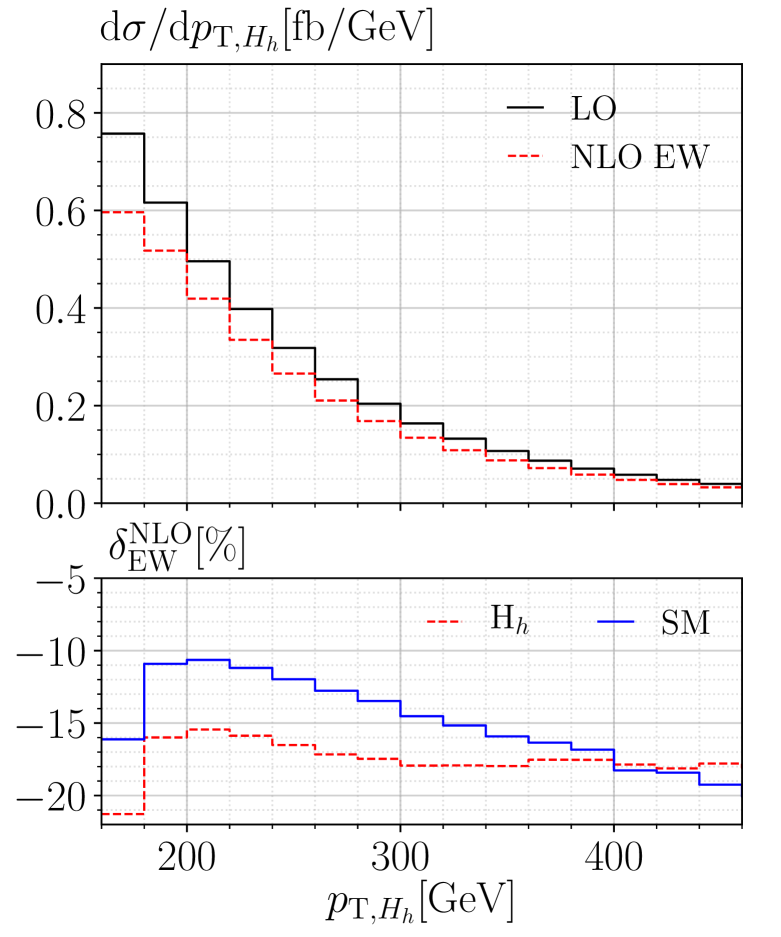
(a) BP3B1 (2HDM)
.

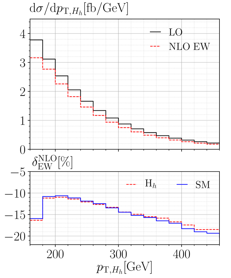
(b) BP45 (2HDM)
.

(c) BP43 (2HDM)

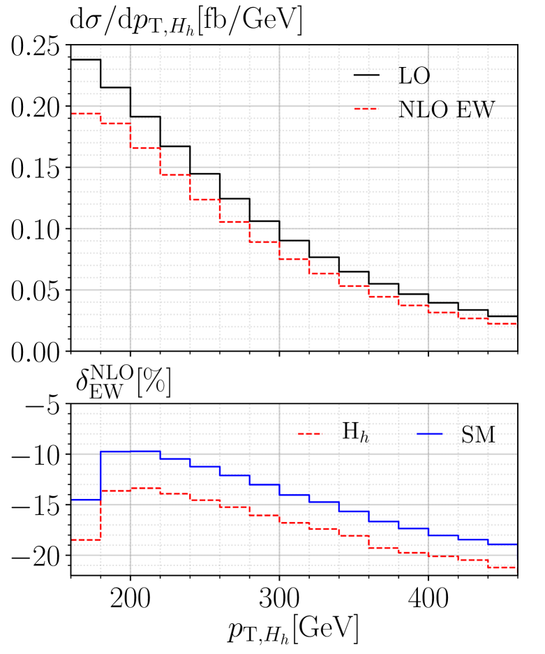
(d) BP3 (HSESM)

Figure 3: Distributions in the transverse momentum of the Higgs boson $p_{\mathrm{T},H_{\mathrm{h}}}$ for heavy Higgs production in Higgs strahlung for the benchmark points BP3B1 in (a), BP45 in (b) and BP43 in (c) in the 2HDM, and BP3 in (d) in the HSESM.

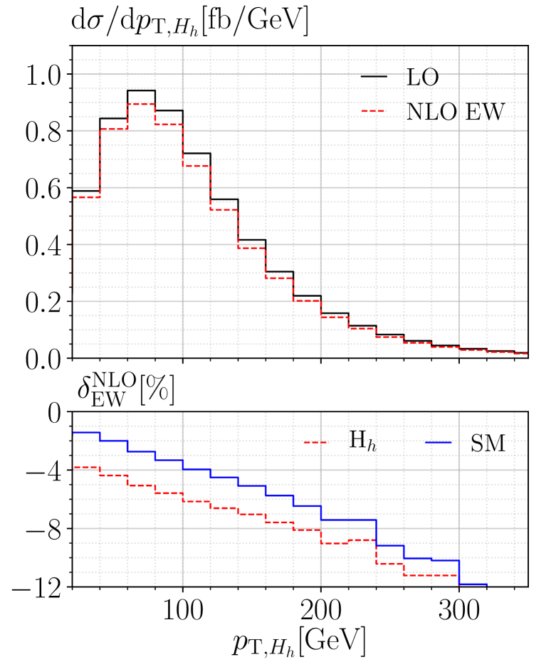
(a) BP3B1 (2HDM)
.

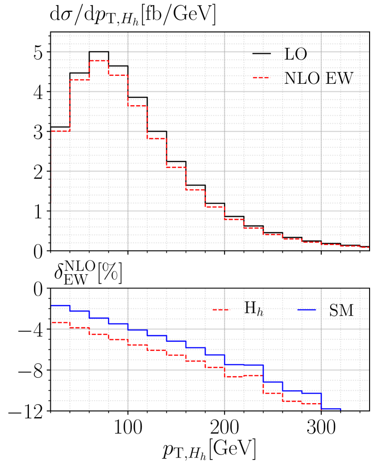
(b) BP45 (2HDM)
.

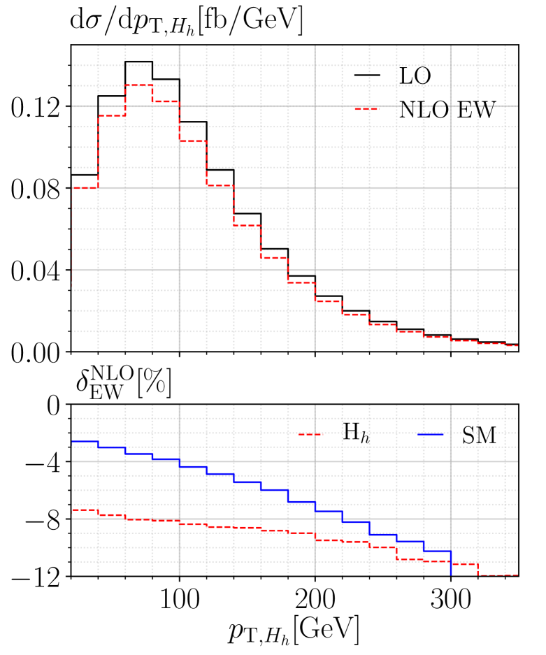
(c) BP43 (2HDM)

(d) BP3 (HSESM)

Figure 4: Distributions in the transverse momentum of the Higgs boson $p_{\mathrm{T},H_{\mathrm{h}}}$ for heavy Higgs production in VBF for the benchmark points BP3B1 in (a), BP45 in (b) and BP43 in (c) in the 2HDM, and BP3 in (d) in the HSESM.

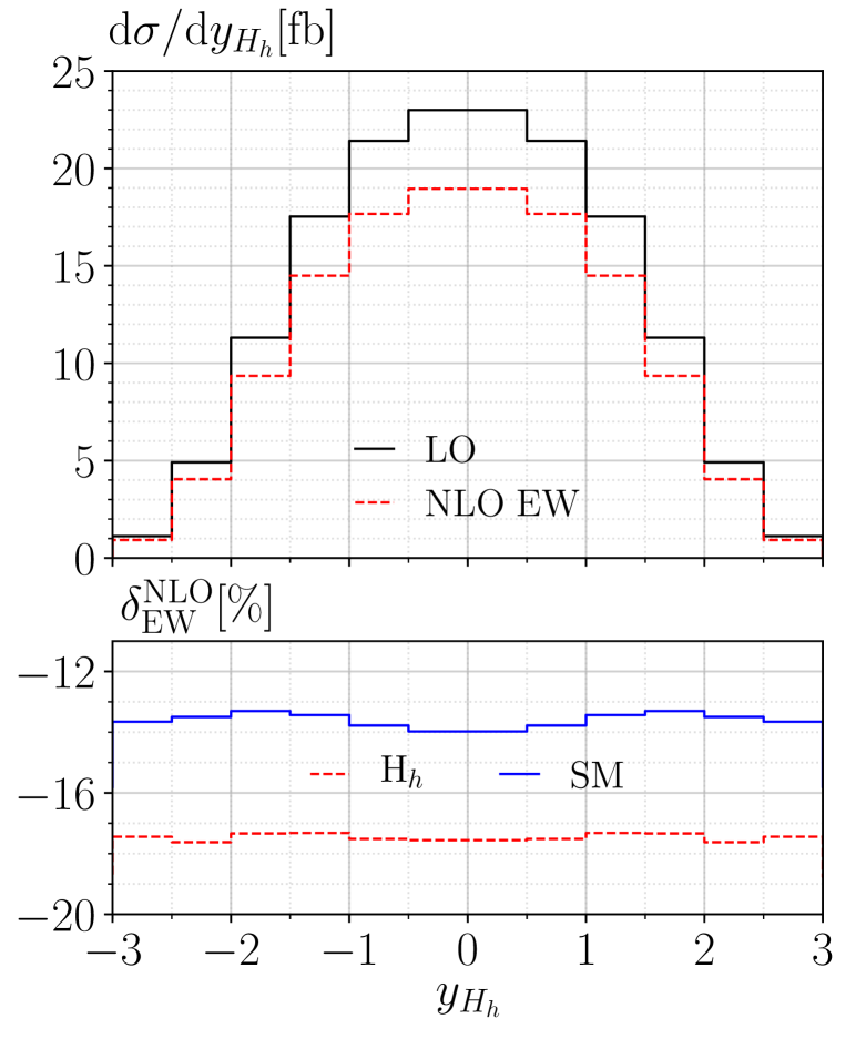
(a) BP3B1 (2HDM)
.

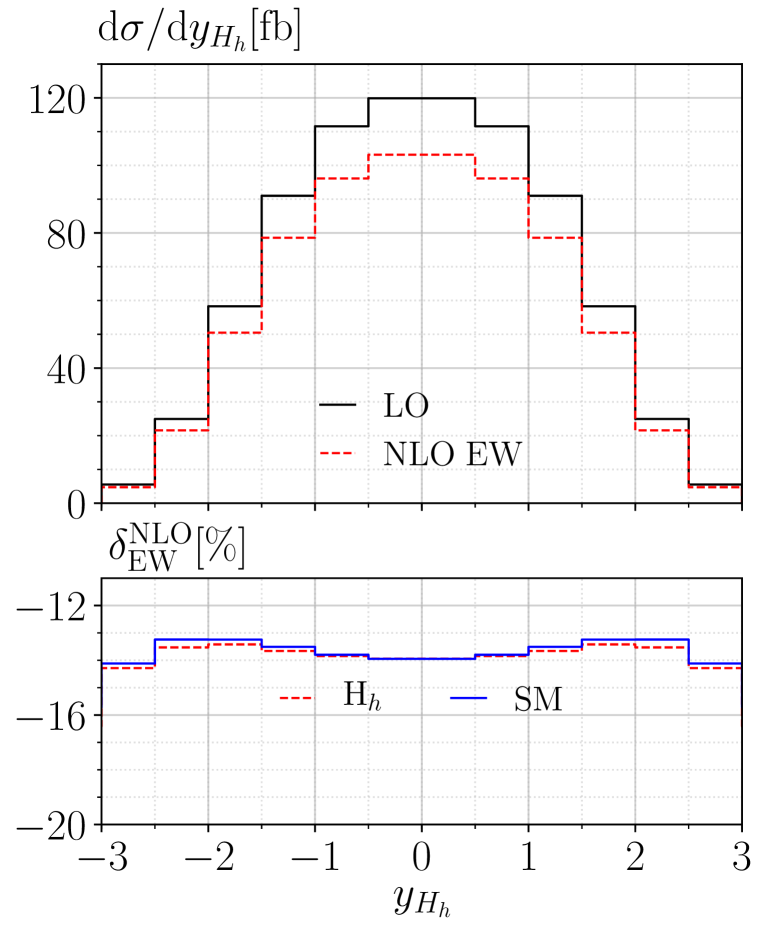
(b) BP45 (2HDM)
.

(c) BP43 (2HDM)

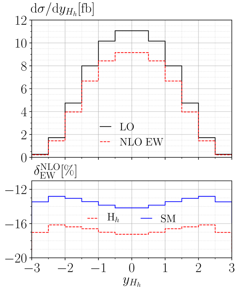
(d) BP3 (HSESM)

Figure 5: Distributions in the rapidity of the Higgs boson $y_{H_{\mathrm{h}}}$ for heavy Higgs production in Higgs strahlung for the benchmark points BP3B1 in (a), BP45 in (b) and BP43 in (c) in the 2HDM, and BP3 in (d) in the HSESM.

(a) BP3B1 (2HDM)
.

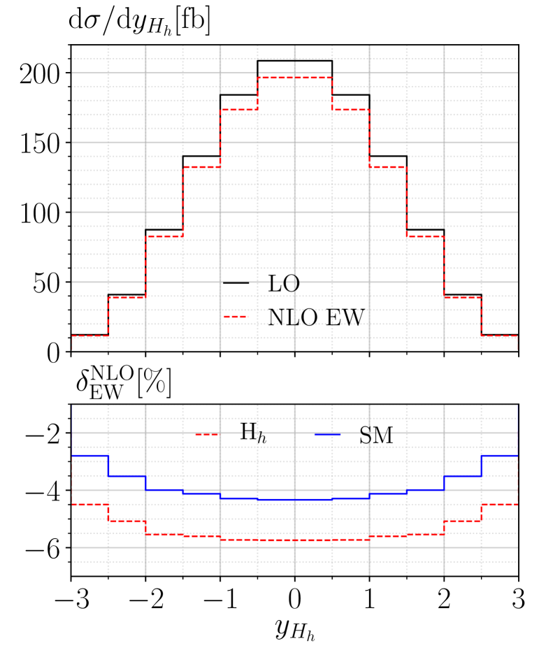
(b) BP45 (2HDM)
.

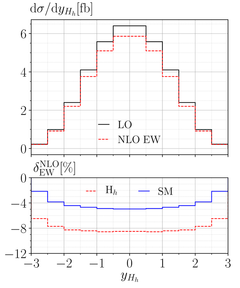
(c) BP43 (2HDM)

(d) BP3 (HSESM)

Figure 6: Distributions in the rapidity of the Higgs boson $y_{H_{\mathrm{h}}}$ for heavy Higgs production in VBF for the benchmark points BP3B1 in (a), BP45 in (b) and BP43 in (c) in the 2HDM, and BP3 in (d) in the HSESM.

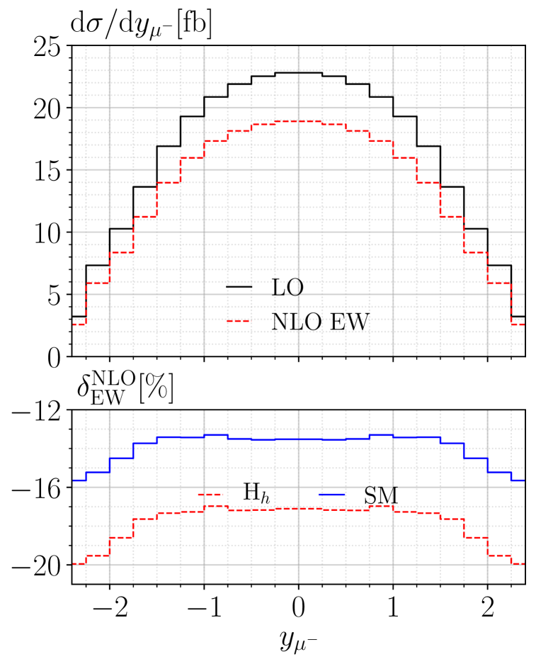
(a) BP3B1 (2HDM)
.

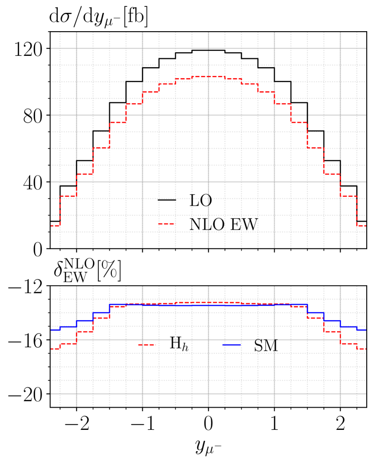
(b) BP45 (2HDM)
.

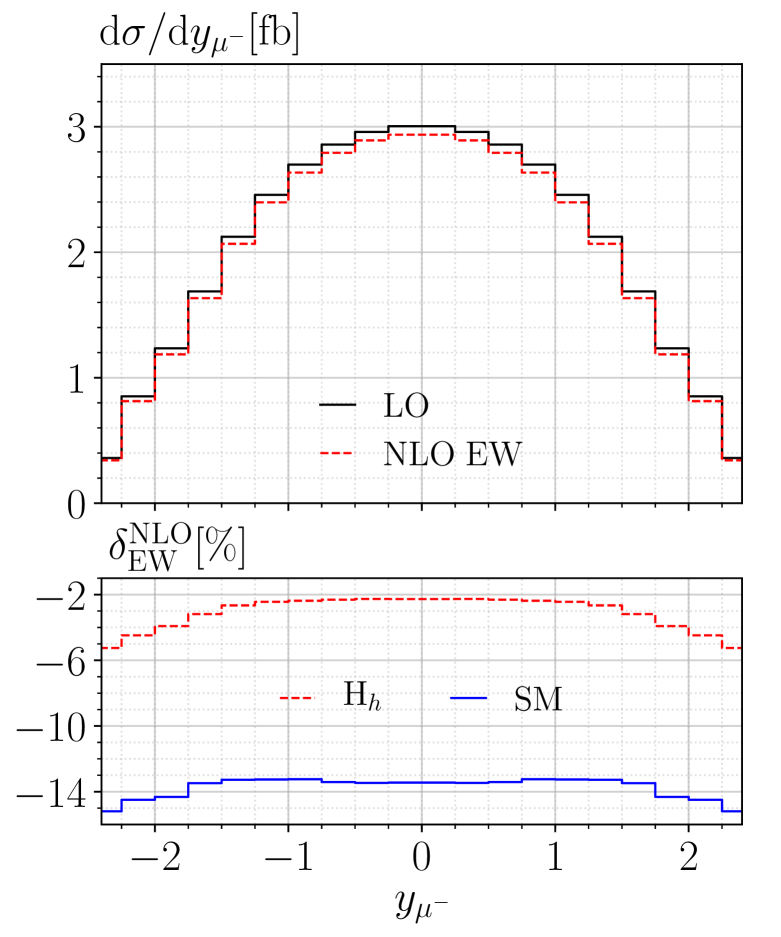
(c) BP43 (2HDM)

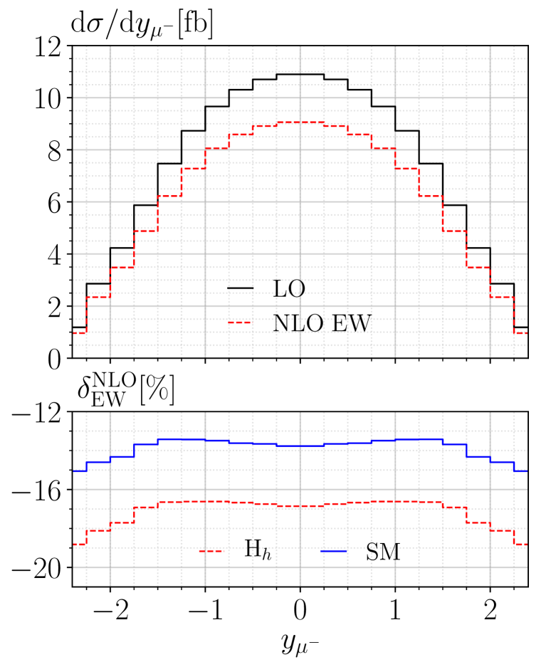
(d) BP3 (HSESM)

Figure 7: Distributions in the rapidity of the muon $y_{\mathrm{\mu}^{-}}$ for heavy Higgs production in Higgs strahlung for the benchmark points BP3B1 in (a), BP45 in (b) and BP43 in (c) in the 2HDM, and BP3 in (d) in the HSESM.

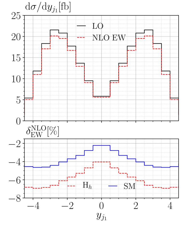
(a) BP3B1 (2HDM)
.

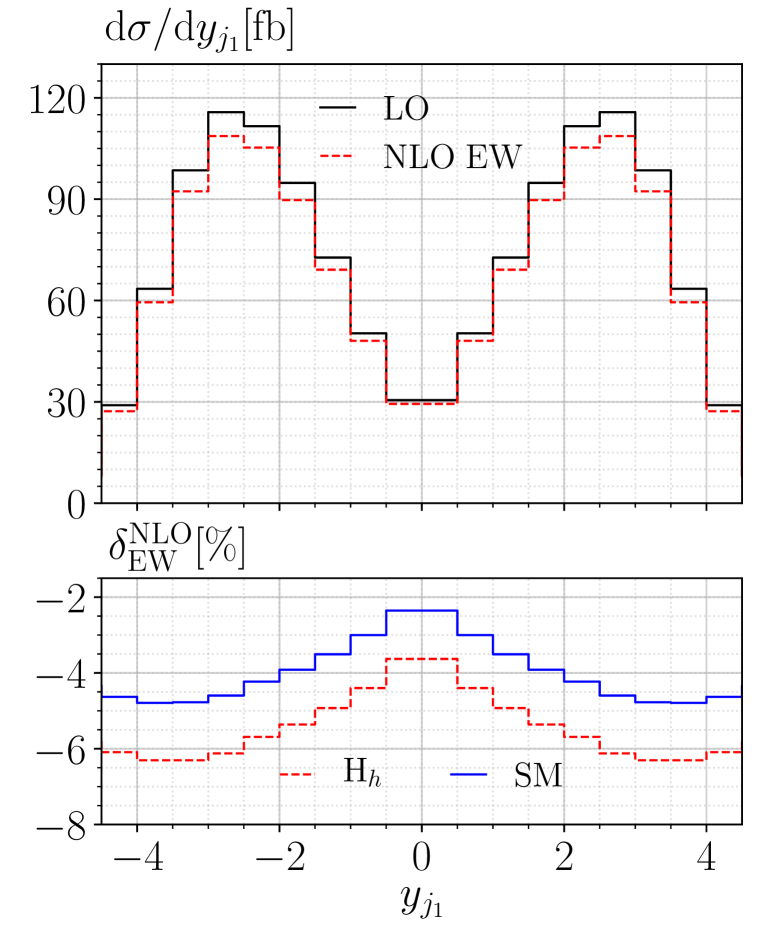
(b) BP45 (2HDM)
.

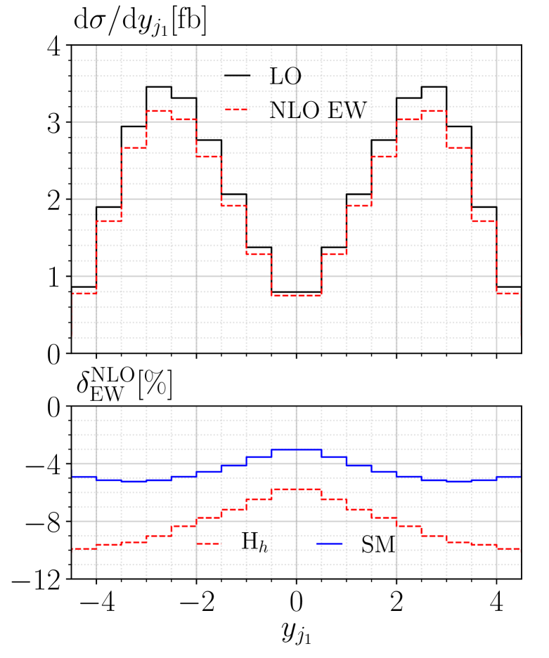
(c) BP43 (2HDM)

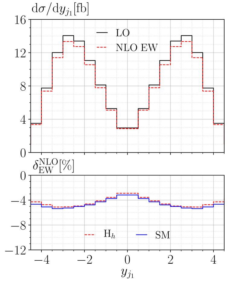
(d) BP3 (HSESM)

Figure 8: Distributions in the rapidity of hardest jet $y_{j_{1}}$ for heavy Higgs production in VBF for the benchmark points BP3B1 in (a), BP45 in (b) and BP43 in (c) in the 2HDM, and BP3 in (d) in the HSESM.

In the following we focus on shape-distortion effects relative to the SM results. Starting with the distributions in Higgs strahlung, we observe quite large effects in the $p_{\mathrm{T},H_{\mathrm{h}}}$ distribution in Fig. 3 for BP3B1 and BP43 in the 2HDM, small effects for BP3 in the HSESM, and no effect in BP45 in the 2HDM, which perfectly reproduces the SM result. The situation changes for the distributions in the rapidities $y_{H_{\mathrm{h}}}$ and $y_{\mu^{-}}$ in Figs. 5 and 7. Here, the largest deviations from the SM are observed for BP43, where the relative EW corrections to the $y_{H_{\mathrm{h}}}$ distribution in the 2HDM are flatter than in the SM. For the $y_{\mu^{-}}$ curve the opposite tendency is observed, i.e. the SM correction is flatter. For BP3B1, BP45, and BP3 shape distortions relative to the SM appear at large rapidities, which are less important due to low statistics in those regions. Switching to the distributions for VBF in Figs. 4, 6, and 8, we observe a stronger trend towards SM-like results. The largest differences are observed for BP43 in the $p_{\mathrm{T},H_{\mathrm{h}}}$ and $y_{j_{1}}$ distributions. For BP3B1 the effects for the same distributions are smaller but significant. For BP3 the shape distortion in the $p_{\mathrm{T},H_{\mathrm{h}}}$ distribution for VBF is not larger than the one for Higgs strahlung. In general in the considered benchmark points for the HSESM the effects in VBF, but also in Higgs strahlung, are tiny compared to the ones observed in the 2HDM.

The reason for the rather mild effects in the HSESM is due to the similiarity of the $\mathrm{H}\mathrm{V}\mathrm{V}$ vertices to the SM ones. In particular, in the HSESM all couplings of the light and heavy Higgs boson to gauge bosons or fermions are SM-like, but modulated with $(-s_{\alpha})$ and $c_{\alpha}$, respectively. In the relative corrections these factors drop out, and the only difference due to the presence of an additional light Higgs boson and modified Higgs-boson couplings is small in the benchmark points under consideration (all $\lambda_{i}\lesssim 1$). Remarkably, even the corrections to the $\mathrm{H}\mathrm{V}\mathrm{V}$ vertices involving Higgs self-couplings (and thus all corrections) scale as the corresponding tree level with either $(-s_{\alpha})$ or $c_{\alpha}$, respectively, in the (anti-)alignment limit. Furthermore, all mixing effects between $H_{\mathrm{l}}$ and $H_{\mathrm{h}}$ vanish in this limit. For these reasons the corrections cannot become enhanced with respect to the LO unless tree-level perturbativity is violated. In fact, in the HSESM the one-loop corrected $H_{\mathrm{h}}\mathrm{V}\mathrm{V}$ vertices are exactly zero in the alignment limit. Note that these arguments apply to the whole phase-space region, thus, no significant shape-distortion effects are expected for the processes under consideration in the HSESM.

The 2HDM, on the other hand, exhibits non-decoupling effects in the alignment limit $c_{\alpha\beta}\to 0$, where the underlying vertices for heavy Higgs-boson production become loop induced. The largest corrections in BP43 are due to the non-decoupling term in the top Yukawa coupling proportional to $s_{\alpha\beta}$. In this case the Yukawa coupling is of the same size as the corresponding SM one, but with a different sign and further enhanced with respect to the LO by a factor of $1/c_{\alpha\beta}$, leading to a non-SM-like bosonic–fermionic interplay. Furthermore, the corrections in the 2HDM are very sensitive to the presence of new particles, especially the pseudo-scalar Higgs boson in the case of BP43. In general, the contributions involving Higgs self-couplings can be large since non-decoupling terms remain in the alignment limit giving rise to enhanced corrections with respect to the LO.

8 Conclusion

We reported progress towards fully automated one-loop computations in BSM models. The presented code RECOLA2 allows one to compute $\mathrm{QCD}$ and $\mathrm{EW}$ corrections for extensions of the SM for arbitrary processes. RECOLA2 can produce NLO corrections in general models, which requires the model file for each BSM model built in a specific format containing the ordinary, counterterm and $R_{2}$ Feynman rules. The model-file generation and the renormalization of general quantum-field-theoretic models is performed with the new tool REPT1L in a fully automated way, relying on nothing but the Feynman rules of the model in the UFO format. Once the renormalization conditions for the model are established, REPT1L performs the renormalization, computes the $R_{2}$ rational terms and builds the one-loop renormalized model files in the RECOLA2 format. We introduced the Background-Field Method as a complementary method in RECOLA2, which is useful for practical calculations and serves as a powerful validation method. We described the renormalization procedure in the Background-Field Method which is handled in RECOLA2 on equal footing with the usual formulation.

In summary, we realized the following generalizations with respect to RECOLA:

• We developed a true model-independent amplitude provider, featuring a dynamic process generation in memory without the need for intermediate compilation.

• A generic interface has been developed supporting all methods available in RECOLA, but generalized to fit in the model-file approach. This includes the computation of amplitudes and squared amplitudes, the selection of specific polarizations and resonances, and the computation of interferences with different powers in new fundamental couplings. Furthermore, we provide spin- and colour-correlated squared matrix elements required in the Catani–Seymour dipole formalism. The latter methods are restricted to singlet, triplet and octet states of SU(3).

• RECOLA2 is limited to scalars, Dirac fermions and vector bosons. In the near future we will allow for Majorana fermions.

• We support Feynman rules with a general polynomial momentum dependence and allow for elementary interactions between more than four fields. Due to internal optimizations the number of fields per elementary interaction is restricted to at most 8.

• We generalized RECOLA2 to support the BFM as a complementary method. Furthermore, the $\mathrm{R}_{\xi}$-gauge can be used for massive vector bosons or, alternatively, non-linear gauges can be implemented.

• With REPT1L we have formed the basis for a fully automated generation of renormalized model files for RECOLA2. We provide a simple framework for the implementation of custom renormalization conditions. Presently available model files for RECOLA2 include the $Z_{2}$-symmetric Two-Higgs-Doublet Model with all types of Yukawa interactions and the Higgs-Singlet extension of the Standard Model as well as models files with anomalous triple vector-boson and Higgs–vector-boson couplings.

The considered simple models do by far not exhaust the range of applicability of RECOLA2 and REPT1L, and further models will be implemented in the future.

As an application of the new tools we present first results for NLO electroweak corrections to vector-boson fusion and updated results for Higgs strahlung in the Two-Higgs-Doublet Model and the Higgs-Singlet extension of the Standard Model. We compared Higgs-production cross sections for different renormalization schemes in both models. We analysed the scale dependence in an ${\overline{\mathrm{MS}}}$ renormalization scheme for the mixing angles, which has been improved including the renormalization-group running of parameters. We found unnaturally large corrections and scale uncertainties at one-loop order for the ${\overline{\mathrm{MS}}}$ scheme, while the considered on-shell schemes remain well-behaved. These enhanced contributions can be related to uncancelled finite parts in the ${\overline{\mathrm{MS}}}$ scheme and should be investigated in more detail in the future, since a proper estimation of higher-order uncertainties, as it can be done based on scale variation in ${\overline{\mathrm{MS}}}$ schemes, is highly desirable. For the on-shell schemes, our results for the electroweak corrections to SM-like Higgs-boson production are almost not distinguishable from the corresponding SM corrections for all considered benchmark points. Finally, we presented distributions for the production of heavy Higgs bosons. Here, interesting shape-distortion effects for the electroweak corrections at the level of several percent are observed in the 2HDM.

9 Acknowledgements

We thank L. Altenkamp for an independent check of $H_{\mathrm{l}}\to 4f$ in the 2HDM which is closely related to the Higgs-production processes considered in this work. We thank L. Jenniches and C. Sturm for valuable discussions and an independent check of the running of $t_{\beta}$ and $c_{\alpha\beta}$. A. D. and J.-N. L. acknowledge support from the German Research Foundation (DFG) via grants DE 623/4-1 and DE 623/5-1. The work of J.-N. L. is supported by the Studienstiftung des deutschen Volkes. The work of S.U. was supported in part by the European Commission through the “HiggsTools” Initial Training Network PITN-GA-2012-316704.

Appendix A Colour-flow vertices

In RECOLA2 the colour flow is constructed recursively. For a given off-shell current the outgoing colour configuration is determined from the incoming ones and the possible colour flows associated to the interaction vertex. As the UFO format does not incorporate the colour flow, we need to translate between the two representations. We implemented a dynamical system for computing the colour flow from the generators and structure constants, rather than substituting for known results. In the conventions of Ref. [10] the colour flow associated to a given colour structure

$$C_{a_{1},\ldots,}{}^{i_{1},\ldots}_{j_{1},\ldots}$$ (A.1)

is obtained by multiplying (A.1) with the normalized generator ${(\Delta_{a_{p}})^{i_{p}}}_{j_{p}}$ for each index $a_{p}$ corresponding to an open index in adjoint representation. The indices $i_{p}$ and $j_{p}$ refer to the colour and anti-colour indices, respectively. The generators $(\Delta_{a})^{i}_{j}$ and structure constants $f_{abc}$ define the SU(3) Lie algebra

$$\left[\Delta_{a},\Delta_{b}\right]=\mathrm{i}\sqrt{2}f_{abc}\Delta_{c},\quad\mathrm{Tr}\left\{\Delta_{a}\Delta_{b}\right\}=\delta_{ab},\quad\Delta_{a}=\frac{\lambda_{a}}{\sqrt{2}},$$ (A.2)

with $\lambda_{a}$ being the Gell-Mann matrices. The computation then consists of eliminating the structure constants and the generators by solving (A.2) for the structure constants and using the (Fierz) completeness relation for the generators as follows

$$f_{abc} =-\frac{1}{\sqrt{2}}\mathrm{i}\mathrm{Tr}\left\{\Delta_{a}\left[\Delta_{b},\Delta_{c}\right]\right\},$$

$$\sum_{a}{\left(\Delta_{a}\right)^{i_{1}}}_{j_{1}}{\left(\Delta_{a}\right)^{i_{2}}}_{j_{2}} =\delta^{i_{1}}_{j_{2}}\delta^{i_{2}}_{j_{1}}-\frac{1}{3}\delta^{i_{1}}_{j_{1}}\delta^{i_{2}}_{j_{2}}.$$ (A.3)

Performing all contractions yields a sum of Kronecker deltas which represent the individual colour flows. For instance, the quartic gluon vertex of the SM reads

$$g_{s}^{2}\sum_{k}\left(f_{ka_{1}a_{2}}f_{ka_{3}a_{4}}L_{1}^{\mu_{1}\mu_{2}\mu_{3}\mu_{4}}+f_{ka_{1}a_{3}}f_{ka_{2}a_{4}}L_{2}^{\mu_{1}\mu_{2}\mu_{3}\mu_{4}}+f_{ka_{1}a_{4}}f_{ka_{2}a_{3}}L_{3}^{\mu_{1}\mu_{2}\mu_{3}\mu_{4}}\right),$$ (A.4)

with $L_{1},L_{2},L_{3}$ being Lorentz structures which, for the following discussion, are left unspecified. Focusing on the colour structure $\delta^{i_{1}}_{j_{2}}\delta^{i_{2}}_{j_{3}}\delta^{i_{3}}_{j_{4}}\delta^{i_{4}}_{j_{1}}$, we obtain for the two relevant contributions

$$\sum_{k,a_{1},a_{2},a_{3},a_{4}}{\left(\Delta_{a_{1}}\right)^{i_{1}}}_{j_{1}}{\left(\Delta_{a_{2}}\right)^{i_{2}}}_{j_{2}}{\left(\Delta_{a_{3}}\right)^{i_{3}}}_{j_{3}}{\left(\Delta_{a_{4}}\right)^{i_{4}}}_{j_{4}}f_{ka_{1}a_{2}}f_{ka_{3}a_{4}}=\frac{1}{2}\left(-\delta^{i_{1}}_{j_{2}}\delta^{i_{2}}_{j_{3}}\delta^{i_{3}}_{j_{4}}\delta^{i_{4}}_{j_{1}}+\ldots\right),$$

$$\sum_{k,a_{1},a_{2},a_{3},a_{4}}{\left(\Delta_{a_{1}}\right)^{i_{1}}}_{j_{1}}{\left(\Delta_{a_{2}}\right)^{i_{2}}}_{j_{2}}{\left(\Delta_{a_{3}}\right)^{i_{3}}}_{j_{3}}{\left(\Delta_{a_{4}}\right)^{i_{4}}}_{j_{4}}f_{ka_{1}a_{4}}f_{ka_{2}a_{3}}=\frac{1}{2}\left(+\delta^{i_{1}}_{j_{2}}\delta^{i_{2}}_{j_{3}}\delta^{i_{3}}_{j_{4}}\delta^{i_{4}}_{j_{1}}+\ldots\right).$$ (A.5)

Combining this result with (A.4), results in the contribution

$$\delta^{i_{1}}_{j_{2}}\delta^{i_{2}}_{j_{3}}\delta^{i_{3}}_{j_{4}}\delta^{i_{4}}_{j_{1}}\times\frac{g_{s}^{2}}{2}\left(L_{3}-L_{1}\right).$$ (A.6)

Thus, diagonalizing the vertex in colour-flow basis requires, in general, to redefine Lorentz structures and couplings.

Appendix B Off-shell currents

For a given Lorentz structure and a definite colour-flow state the $\mathrm{BGR}$ is derived from the Feynman rules by selecting one of the particles as the outgoing one, multiplying with the corresponding propagator and the incoming currents of the other particles. Since the structure of currents depends on the outgoing particle, one needs to derive the $\mathrm{BGR}$ for all distinct outgoing particles. Consider for instance the $\mathrm{QED}$ vertex $\mathrm{e}^{+}\mathrm{e}^{-}\gamma$. REPT1L constructs three different recursion relations

$$w_{\alpha}=\mathrm{i}e\sum_{\beta,\delta,\mu}D^{e^{-}}_{\alpha\beta}\left(\gamma^{\mu}\right)_{\beta\delta}\times w_{\mu}\times w_{\delta},$$

$$\bar{w}_{\beta}=\mathrm{i}e\sum_{\alpha,\delta,\mu}D^{e^{+}}_{\alpha\beta}\left(\gamma^{\mu}\right)_{\delta\alpha}\times w_{\mu}\times\bar{w}_{\delta},$$

$$w_{\mu}=\mathrm{i}e\sum_{\alpha,\beta,\nu}D^{\gamma}_{\mu\nu}\left(\gamma^{\nu}\right)_{\alpha\beta}\times\bar{w}_{\alpha}\times w_{\beta},$$ (B.1)

with $w_{i},\bar{w}_{j},w_{\mu}$ being either incoming or outgoing off-shell currents, depending on whether they are on the right- or left-hand side of (B.1). For many Feynman rules, the underlying $\mathrm{BGR}$ are formally the same if the couplings or masses of the particles are not further specified. Assuming that the colour flow has been factorized as explained in App. A, all fermion–fermion–vector rules, e.g. $\mathrm{Z}\mathrm{e}\to\mathrm{e}$ or $\gamma\mathrm{e}\to\mathrm{e}$, can be mapped onto the same structures realizing that $\gamma^{\mu}\omega^{+}$ and $\gamma^{\mu}\omega^{-}$ form a suitable basis,

$$w_{\alpha} =\sum_{\beta,\delta,\mu}D_{\alpha\beta}^{f}\left(c_{1}\gamma^{\mu}\omega^{+}+c_{2}\gamma^{\mu}\omega^{-}\right)_{\beta\delta}\times w_{\mu}\times w_{\delta},$$

$$\bar{w}_{\beta} =\sum_{\alpha,\delta,\mu}D_{\alpha\beta}^{\bar{f}}\left(c_{1}\gamma^{\mu}\omega^{+}+c_{2}\gamma^{\mu}\omega^{-}\right)_{\delta\alpha}\times w_{\mu}\times\bar{w}_{\delta},$$

$$w_{\mu} =\sum_{\alpha,\beta,\nu}D_{\mu\nu}^{V}\left(c_{1}\gamma^{\nu}\omega^{+}+c_{2}\gamma^{\nu}\omega^{-}\right)_{\alpha\beta}\times\bar{w}_{\alpha}\times w_{\beta},$$ (B.2)

with $D_{\alpha\beta}^{f},D_{\alpha\beta}^{\bar{f}},D_{\mu\nu}^{V}$ denoting generic propagators for fermions, anti-fermions and vector bosons, respectively. REPT1L has the ability to derive a minimal basis, dynamically, i.e. depending on the operators of the theory, without relying on the Lorentz basis in the UFO format. This is done in two steps. In the first step, all distinct $\mathrm{BGR}$ in the underlying theory are registered. In the next step the $\mathrm{BGR}$ are merged recursively until a minimal basis is obtained. The size of the $\mathrm{BGR}$ can be controlled by a parameter for the maximal number of allowed distinct generic couplings, and it is possible to allow for vanishing couplings to improve the merging. If a merge yields a $\mathrm{BGR}$ size larger than allowed, the merging is not accepted. Finally, all vertices are mapped to the minimal basis.

Appendix C Translation of $\delta\alpha$ to other tadpole schemes

In this section we discuss the translation of on-shell renormalization conditions from one tadpole counterterm scheme to others using the example of $\delta\alpha$ renormalized in the $p^{*}$ scheme (6.8). Once, we treat the tadpole counterterms in the FJ Tadpole Scheme, with the tadpole renormalization (5.30). As an alternative tadpole counterterm scheme, we consider the one of Ref. [51], denoted as scheme S1, which is commonly used in the SM. In S1 the tadpole counterterm to the neutral scalar mixing energy is zero. Then, $\delta\alpha_{\mathrm{S1}}$ in the $p^{*}$ scheme is consistently defined by absorbing all tadpole contributions as

$$\delta\alpha_{\mathrm{S1}} =\delta\alpha-\frac{t_{H_{\mathrm{l}}H_{\mathrm{h}}}}{M_{H_{\mathrm{h}}}^{2}-M_{H_{\mathrm{l}}}^{2}}$$ (C.1)

with $\delta\alpha$ and $t_{H_{\mathrm{l}}H_{\mathrm{h}}}$ being evaluated in the FJ Tadpole Scheme together with the tadpole renormalization (5.30). Note that (C.1) holds in any gauge, but only the tadpole $t_{H_{\mathrm{l}}H_{\mathrm{h}}}$ is affected by the gauge choice, as $\delta\alpha$ is defined as gauge-parameter independent. For the ’t Hooft–Feynman gauge (C.1) reduces to

$$\delta\alpha_{S1}=\frac{\Sigma^{\mathrm{1PI},\mathrm{BFM}}_{H_{\mathrm{h}}H_{\mathrm{l}}}\left(\frac{M_{H_{\mathrm{h}}}^{2}+M_{H_{\mathrm{l}}}^{2}}{2}\right)}{M_{H_{\mathrm{h}}}^{2}-M_{H_{\mathrm{l}}}^{2}}.$$ (C.2)

In order to verify the gauge independence of the $S$-matrix one has to use the gauge dependence originating exclusively from the absorbed tadpoles. Equation (C.1) implies for the gauge-parameter dependence of $\delta\alpha_{S1}$

$$\frac{\partial\delta\alpha_{S1}}{\partial\xi}=-\frac{1}{M_{H_{\mathrm{h}}}^{2}-M_{H_{\mathrm{l}}}^{2}}\frac{\partial t_{H_{\mathrm{l}}H_{\mathrm{h}}}}{\partial\xi},$$ (C.3)

with $\xi$ generically denoting a parametrization of a gauge choice, not necessarily $\mathrm{R}_{\xi}$ gauge. We stress that the gauge dependence of (C.3) is not equivalent to the gauge dependence of the mixing energy (C.2). Finally, when studying the gauge dependence of $S$-matrix elements, the gauge dependence (C.3) necessarily cancels against the tadpole counterterm gauge dependence absorbed in other on-shell renormalized counterterms, e.g. mass counterterms and $\delta t_{\beta}$ (and $\delta M_{\rm sb}^{2}$ in the 2HDM).

References

- [1] CMS Collaboration, S. Chatrchyan et al., Observation of a new boson at a mass of 125 GeV with the CMS experiment at the LHC, Phys. Lett. B716 (2012) 30–61, [arXiv:1207.7235].
- [2] ATLAS Collaboration, G. Aad et al., Observation of a new particle in the search for the Standard Model Higgs boson with the ATLAS detector at the LHC, Phys. Lett. B716 (2012) 1–29, [arXiv:1207.7214].
- [3] S. Kallweit, J. M. Lindert, P. Maierhöfer, S. Pozzorini, and M. Schönherr, NLO electroweak automation and precise predictions for W+multijet production at the LHC, JHEP 04 (2015) 012, [arXiv:1412.5157].
- [4] J. Alwall, et al., The automated computation of tree-level and next-to-leading order differential cross sections, and their matching to parton shower simulations, JHEP 07 (2014) 079, [arXiv:1405.0301].
- [5] G. Cullen et al., GoSam-2.0: a tool for automated one-loop calculations within the Standard Model and beyond, Eur. Phys. J. C74 (2014), no. 8 3001, [arXiv:1404.7096].
- [6] M. Chiesa, N. Greiner, and F. Tramontano, Automation of electroweak corrections for LHC processes, J. Phys. G43 (2016), no. 1 013002, [arXiv:1507.08579].
- [7] T. Hahn, Generating Feynman diagrams and amplitudes with FeynArts 3, Comput. Phys. Commun. 140 (2001) 418–431, [hep-ph/0012260].
- [8] C. Groß, et al., New Developments in FormCalc 8.4, arXiv:1407.0235. [PoSLL2014,035(2014)].
- [9] S. Actis, A. Denner, L. Hofer, A. Scharf, and S. Uccirati, Recursive generation of one-loop amplitudes in the Standard Model, JHEP 04 (2013) 037, [arXiv:1211.6316].
- [10] S. Actis, et al., RECOLA: REcursive Computation of One-Loop Amplitudes, Comput. Phys. Commun. 214 (2017) 140–173, [arXiv:1605.01090].
- [11] A. Alloul, N. D. Christensen, C. Degrande, C. Duhr, and B. Fuks, FeynRules 2.0 - A complete toolbox for tree-level phenomenology, Comput. Phys. Commun. 185 (2014) 2250–2300, [arXiv:1310.1921].
- [12] F. Staub, SARAH 4: A tool for (not only SUSY) model builders, Comput. Phys. Commun. 185 (2014) 1773–1790, [arXiv:1309.7223].
- [13] C. Degrande, Automatic evaluation of UV and R2 terms for beyond the Standard Model Lagrangians: a proof-of-principle, Comput. Phys. Commun. 197 (2015) 239–262, [arXiv:1406.3030].
- [14] C. Degrande, et al., UFO - The Universal FeynRules Output, Comput. Phys. Commun. 183 (2012) 1201–1214, [arXiv:1108.2040].
- [15] R. Hamberg, W. L. van Neerven, and T. Matsuura, A complete calculation of the order correction to the Drell-Yan factor, Nucl. Phys. B359 (1991) 343–405. [Erratum: Nucl. Phys. B644 (2002) 403].
- [16] O. Brein, A. Djouadi, and R. Harlander, NNLO QCD corrections to the Higgs-strahlung processes at hadron colliders, Phys. Lett. B579 (2004) 149–156, [hep-ph/0307206].
- [17] O. Brein, R. Harlander, M. Wiesemann, and T. Zirke, Top-quark mediated effects in hadronic Higgs strahlung, Eur. Phys. J. C72 (2012) 1868, [arXiv:1111.0761].
- [18] G. Ferrera, M. Grazzini, and F. Tramontano, Associated WH production at hadron colliders: a fully exclusive QCD calculation at NNLO, Phys. Rev. Lett. 107 (2011) 152003, [arXiv:1107.1164].
- [19] G. Ferrera, M. Grazzini, and F. Tramontano, Associated ZH production at hadron colliders: the fully differential NNLO QCD calculation, Phys. Lett. B740 (2015) 51–55, [arXiv:1407.4747].
- [20] M. L. Ciccolini, S. Dittmaier, and M. Krämer, Electroweak radiative corrections to associated WH and ZH production at hadron colliders, Phys. Rev. D68 (2003) 073003, [hep-ph/0306234].
- [21] A. Denner, S. Dittmaier, S. Kallweit, and A. Mück, Electroweak corrections to Higgs-strahlung off W/Z bosons at the Tevatron and the LHC with HAWK, JHEP 03 (2012) 075, [arXiv:1112.5142].
- [22] R. V. Harlander, S. Liebler, and T. Zirke, Higgs strahlung at the Large Hadron Collider in the 2-Higgs-Doublet Model, JHEP 02 (2014) 023, [arXiv:1307.8122].
- [23] A. Denner, L. Jenniches, J.-N. Lang, and C. Sturm, Gauge-independent renormalization in the 2HDM, JHEP 09 (2016) 115, [arXiv:1607.07352].
- [24] F. Maltoni, K. Mawatari, and M. Zaro, Higgs characterisation via vector-boson fusion and associated production: NLO and parton-shower effects, Eur. Phys. J. C74 (2014), no. 1 2710, [arXiv:1311.1829].
- [25] T. Han, G. Valencia, and S. Willenbrock, Structure function approach to vector boson scattering in p p collisions, Phys. Rev. Lett. 69 (1992) 3274–3277, [hep-ph/9206246].
- [26] P. Bolzoni, F. Maltoni, S.-O. Moch, and M. Zaro, Higgs production via vector-boson fusion at NNLO in QCD, Phys. Rev. Lett. 105 (2010) 011801, [arXiv:1003.4451].
- [27] P. Bolzoni, F. Maltoni, S.-O. Moch, and M. Zaro, Vector boson fusion at NNLO in QCD: SM Higgs and beyond, Phys. Rev. D85 (2012) 035002, [arXiv:1109.3717].
- [28] T. Figy, C. Oleari, and D. Zeppenfeld, Next-to-leading order jet distributions for Higgs boson production via weak boson fusion, Phys. Rev. D68 (2003) 073005, [hep-ph/0306109].
- [29] M. Ciccolini, A. Denner, and S. Dittmaier, Electroweak and QCD corrections to Higgs production via vector-boson fusion at the LHC, Phys. Rev. D77 (2008) 013002, [arXiv:0710.4749].
- [30] M. Ciccolini, A. Denner, and S. Dittmaier, Strong and electroweak corrections to the production of Higgs + 2jets via weak interactions at the LHC, Phys. Rev. Lett. 99 (2007) 161803, [arXiv:0707.0381].
- [31] M. Cacciari, F. A. Dreyer, A. Karlberg, G. P. Salam, and G. Zanderighi, Fully Differential Vector-Boson-Fusion Higgs Production at Next-to-Next-to-Leading Order, Phys. Rev. Lett. 115 (2015), no. 8 082002, [arXiv:1506.02660].
- [32] F. A. Dreyer and A. Karlberg, Vector-Boson Fusion Higgs Production at Three Loops in QCD, Phys. Rev. Lett. 117 (2016), no. 7 072001, [arXiv:1606.00840].
- [33] S. Frixione, P. Torrielli, and M. Zaro, Higgs production through vector-boson fusion at the NLO matched with parton showers, Phys. Lett. B726 (2013) 273–282, [arXiv:1304.7927].
- [34] M. Rauch and S. Plätzer, Parton-shower Effects in Vector-Boson-Fusion Processes, PoS DIS2016 (2016) 076, [arXiv:1607.00159].
- [35] D. Goncalves, T. Plehn, and J. M. Thompson, Weak Boson Fusion at 100 TeV, arXiv:1702.05098.
- [36] T. Figy, S. Palmer, and G. Weiglein, Higgs Production via Weak Boson Fusion in the Standard Model and the MSSM, JHEP 02 (2012) 105, [arXiv:1012.4789].
- [37] M. Spira, V2HV, http://tiger.web.psi.ch/proglist.html.
- [38] J. Campbell, K. Ellis, and C. Williams, MCFM–Monte Carlo for FeMtobarn processes, http://mcfm.fnal.gov/.
- [39] A. Denner, S. Dittmaier, S. Kallweit, and A. Mück, HAWK 2.0: A Monte Carlo program for Higgs production in vector-boson fusion and Higgs strahlung at hadron colliders, Comput. Phys. Commun. 195 (2015) 161–171, [arXiv:1412.5390].
- [40] O. Brein, R. V. Harlander, and T. J. E. Zirke, vh@nnlo - Higgs strahlung at hadron colliders, Comput. Phys. Commun. 184 (2013) 998–1003, [arXiv:1210.5347].
- [41] F. J. Dyson, The S matrix in quantum electrodynamics, Phys. Rev. 75 (1949) 1736–1755.
- [42] J. S. Schwinger, On the Green’s functions of quantized fields. 1., Proc. Nat. Acad. Sci. 37 (1951) 452–455.
- [43] J. S. Schwinger, On the Green’s functions of quantized fields. 2., Proc. Nat. Acad. Sci. 37 (1951) 455–459.
- [44] A. Kanaki and C. G. Papadopoulos, HELAC: A Package to compute electroweak helicity amplitudes, Comput. Phys. Commun. 132 (2000) 306–315, [hep-ph/0002082].
- [45] A. van Hameren, Multi-gluon one-loop amplitudes using tensor integrals, JHEP 0907 (2009) 088, [arXiv:0905.1005].
- [46] A. Denner, S. Dittmaier, and L. Hofer, Collier: a fortran-based Complex One-Loop LIbrary in Extended Regularizations, Comput. Phys. Commun. 212 (2017) 220–238, [arXiv:1604.06792].
- [47] F. A. Berends and W. T. Giele, Recursive Calculations for Processes with n Gluons, Nucl. Phys. B306 (1988) 759–808.
- [48] F. Caravaglios and M. Moretti, An algorithm to compute Born scattering amplitudes without Feynman graphs, Phys. Lett. B358 (1995) 332–338, [hep-ph/9507237].
- [49] J. A. M. Vermaseren, New features of FORM, math-ph/0010025.
- [50] A. Meurer, et al., Sympy: symbolic computing in python, PeerJ Computer Science 3 (Jan., 2017) e103.
- [51] A. Denner, Techniques for calculation of electroweak radiative corrections at the one-loop level and results for W physics at LEP-200, Fortsch. Phys. 41 (1993) 307–420, [arXiv:0709.1075].
- [52] G. Ossola, C. G. Papadopoulos, and R. Pittau, On the Rational Terms of the one-loop amplitudes, JHEP 05 (2008) 004, [arXiv:0802.1876].
- [53] P. Draggiotis, M. V. Garzelli, C. G. Papadopoulos, and R. Pittau, Feynman Rules for the Rational Part of the QCD 1-loop amplitudes, JHEP 04 (2009) 072, [arXiv:0903.0356].
- [54] M. V. Garzelli, I. Malamos, and R. Pittau, Feynman rules for the rational part of the Electroweak 1-loop amplitudes, JHEP 01 (2010) 040, [arXiv:0910.3130]. [Erratum: JHEP10 (2010) 097].
- [55] S. Catani and M. H. Seymour, A General algorithm for calculating jet cross-sections in NLO QCD, Nucl. Phys. B485 (1997) 291–419, [hep-ph/9605323]. [Erratum: Nucl. Phys. B510 (1998) 503].
- [56] S. Catani, S. Dittmaier, M. H. Seymour, and Z. Trocsanyi, The Dipole formalism for next-to-leading order QCD calculations with massive partons, Nucl. Phys. B627 (2002) 189–265, [hep-ph/0201036].
- [57] S. Dittmaier, A General approach to photon radiation off fermions, Nucl. Phys. B565 (2000) 69–122, [hep-ph/9904440].
- [58] S. Dittmaier, A. Kabelschacht, and T. Kasprzik, Polarized QED splittings of massive fermions and dipole subtraction for non-collinear-safe observables, Nucl. Phys. B800 (2008) 146–189, [arXiv:0802.1405].
- [59] J. F. Gunion and H. E. Haber, The CP conserving Two-Higgs-Doublet Model: the approach to the decoupling limit, Phys. Rev. D67 (2003) 075019, [hep-ph/0207010].
- [60] G. C. Branco, et al., Theory and phenomenology of Two-Higgs-Doublet Models, Phys. Rept. 516 (2012) 1–102, [arXiv:1106.0034].
- [61] R. M. Schabinger and J. D. Wells, A Minimal spontaneously broken hidden sector and its impact on Higgs boson physics at the large hadron collider, Phys. Rev. D72 (2005) 093007, [hep-ph/0509209].
- [62] B. Patt and F. Wilczek, Higgs-field portal into hidden sectors, hep-ph/0605188.
- [63] M. Bowen, Y. Cui, and J. D. Wells, Narrow trans-TeV Higgs bosons and H —¿ hh decays: Two LHC search paths for a hidden sector Higgs boson, JHEP 03 (2007) 036, [hep-ph/0701035].
- [64] G. M. Pruna and T. Robens, Higgs singlet extension parameter space in the light of the LHC discovery, Phys. Rev. D88 (2013), no. 11 115012, [arXiv:1303.1150].
- [65] T. Robens and T. Stefaniak, Status of the Higgs Singlet Extension of the Standard Model after LHC Run 1, Eur. Phys. J. C75 (2015) 104, [arXiv:1501.02234].
- [66] T. Robens and T. Stefaniak, LHC Benchmark Scenarios for the Real Higgs Singlet Extension of the Standard Model, Eur. Phys. J. C76 (2016), no. 5 268, [arXiv:1601.07880].
- [67] G. Chalons, D. Lopez-Val, T. Robens, and T. Stefaniak, The Higgs singlet extension at LHC Run 2, in Proceedings, 38th International Conference on High Energy Physics (ICHEP 2016): Chicago, IL, USA, August 3-10, 2016, 2016. arXiv:1611.03007.
- [68] S. L. Glashow and S. Weinberg, Natural Conservation Laws for Neutral Currents, Phys. Rev. D15 (1977) 1958.
- [69] E. A. Paschos, Diagonal Neutral Currents, Phys. Rev. D15 (1977) 1966.
- [70] B. S. DeWitt, Theory of radiative corrections for non-abelian gauge fields, Phys. Rev. Lett. 12 (1964) 742–746.
- [71] B. S. DeWitt, Quantum Theory of Gravity. 2. The Manifestly Covariant Theory, Phys. Rev. 162 (1967) 1195–1239.
- [72] L. F. Abbott, Introduction to the Background Field Method, Acta Phys. Polon. B13 (1982) 33.
- [73] J. P. Bornsen and A. E. M. van de Ven, Three loop Yang-Mills beta function via the covariant background field method, Nucl. Phys. B657 (2003) 257–303, [hep-th/0211246].
- [74] L. F. Abbott, M. T. Grisaru, and R. K. Schaefer, The Background Field Method and the S Matrix, Nucl. Phys. B229 (1983) 372–380.
- [75] A. Denner, G. Weiglein, and S. Dittmaier, Application of the background field method to the electroweak standard model, Nucl. Phys. B440 (1995) 95–128, [hep-ph/9410338].
- [76] A. Sirlin, Radiative corrections in the theory: A simple renormalization framework, Phys. Rev. D22 (1980) 971–981.
- [77] W. J. Marciano and A. Sirlin, Radiative corrections to neutrino induced neutral-current phenomena in the theory, Phys. Rev. D22 (1980) 2695. [Erratum: Phys. Rev. D31 (1985) 213].
- [78] A. Sirlin and W. J. Marciano, Radiative corrections to and their effect on the determination of and , Nucl. Phys. B189 (1981) 442–460.
- [79] A. Denner, S. Dittmaier, M. Roth, and D. Wackeroth, Predictions for all processes fermions , Nucl.Phys. B560 (1999) 33–65, [hep-ph/9904472].
- [80] A. Denner, S. Dittmaier, M. Roth, and L. Wieders, Electroweak corrections to charged-current fermion processes: Technical details and further results, Nucl.Phys. B724 (2005) 247–294, [hep-ph/0505042].
- [81] A. Denner and S. Dittmaier, The Complex-mass scheme for perturbative calculations with unstable particles, Nucl. Phys. Proc. Suppl. 160 (2006) 22–26, [hep-ph/0605312].
- [82] J. Fleischer and F. Jegerlehner, Radiative corrections to Higgs decays in the extended Weinberg-Salam Model, Phys. Rev. D23 (1981) 2001–2026.
- [83] M. Krause, R. Lorenz, M. Mühlleitner, R. Santos, and H. Ziesche, Gauge-independent renormalization of the 2-Higgs-Doublet Model, arXiv:1605.04853.
- [84] Particle Data Group Collaboration, C. Patrignani et al., Review of Particle Physics, Chin. Phys. C40 (2016), no. 10 100001.
- [85] LHC Higgs Cross Section Working Group Collaboration, D. de Florian et al., Handbook of LHC Higgs Cross Sections: 4. Deciphering the Nature of the Higgs Sector, arXiv:1610.07922.
- [86] L. Altenkamp, S. Dittmaier, and H. Rzehak, Renormalization schemes for the Two-Higgs-Doublet Model and applications to fermions, arXiv:1704.02645.
- [87] P. Nogueira, Automatic Feynman graph generation, J. Comput. Phys. 105 (1993) 279–289.
- [88] S. Actis, A. Ferroglia, G. Passarino, M. Passera, Ch. Sturm and S. Uccirati, GraphShot, a Form package for automatic generation and manipulation of one- and two-loop Feynman diagrams, unpublished.
- [89] CMS Collaboration, S. Chatrchyan et al., Search for the Standard Model Higgs boson produced in association with a W or a Z boson and decaying to bottom quarks, Phys. Rev. D89 (2014), no. 1 012003, [arXiv:1310.3687].
- [90] M. Cacciari, G. P. Salam, and G. Soyez, The anti-k(t) jet clustering algorithm, JHEP 04 (2008) 063, [arXiv:0802.1189].
- [91] NNPDF Collaboration, R. D. Ball, et al., Parton distributions with QED corrections, Nucl. Phys. B877 (2013) 290–320, [arXiv:1308.0598].
- [92] LHC Higgs Cross Section Working Group Collaboration, I. Low et al., “Beyond the Standard Model Predictions.” http://cds.cern.ch/record/2150772/files/. Accessed: 2016-06-29.
- [93] J. Baglio, O. Eberhardt, U. Nierste, and M. Wiebusch, Benchmarks for Higgs pair production and heavy Higgs searches in the Two-Higgs-Doublet Model of type II, Phys. Rev. D90 (2014), no. 1 015008, [arXiv:1403.1264].
- [94] F. Bojarski, G. Chalons, D. Lopez-Val, and T. Robens, Heavy to light Higgs boson decays at NLO in the Singlet Extension of the Standard Model, JHEP 02 (2016) 147, [arXiv:1511.08120].
- [95] J. R. Espinosa and I. Navarro, Scale independent mixing angles, Phys. Rev. D66 (2002) 016004, [hep-ph/0109126].
- [96] J. R. Espinosa and Y. Yamada, Scale independent and gauge independent mixing angles for scalar particles, Phys. Rev. D67 (2003) 036003, [hep-ph/0207351].
- [97] A. Denner, G. Weiglein, and S. Dittmaier, Gauge invariance of green functions: Background field method versus pinch technique, Phys. Lett. B333 (1994) 420–426, [hep-ph/9406204].
- [98] D. Binosi, Electroweak pinch technique to all orders, J. Phys. G30 (2004) 1021–1064, [hep-ph/0401182].
- [99] J. M. Cornwall, Dynamical mass generation in continuum QCD, Phys. Rev. D26 (1982) 1453.
- [100] J. M. Cornwall and J. Papavassiliou, Gauge-invariant three gluon vertex in QCD, Phys. Rev. D40 (1989) 3474.
- [101] S. Kanemura, M. Kikuchi, K. Sakurai, and K. Yagyu, Gauge invariant one-loop corrections to Higgs boson couplings in non-minimal Higgs models, arXiv:1705.05399.
- [102] A. Freitas and D. Stöckinger, Gauge dependence and renormalization of in the MSSM, Phys. Rev. D66 (2002) 095014, [hep-ph/0205281].
- [103] J. Brehmer, A. Freitas, D. Lopez-Val, and T. Plehn, Pushing Higgs Effective Theory to its Limits, Phys. Rev. D93 (2016), no. 7 075014, [arXiv:1510.03443].