The Viewing Geometry of Brown Dwarfs Influences Their Observed Colours and Variability Amplitudes
Abstract
In this paper we study the full sample of known Spitzer [m] and -band variable brown dwarfs. We calculate the rotational velocities, , of 16 variable brown dwarfs using archival Keck NIRSPEC data and compute the inclination angles of 19 variable brown dwarfs. The results obtained show that all objects in the sample with mid-IR variability detections are inclined at an angle , while all objects in the sample displaying -band variability have an inclination angle . -band variability appears to be more affected by inclination than Spitzer [m] variability, and is strongly attenuated at lower inclinations. Since -band observations probe deeper into the atmosphere than mid-IR observations, this effect may be due to the increased atmospheric path length of -band flux at lower inclinations. We find a statistically significant correlation between the colour anomaly and inclination of our sample, where field objects viewed equator-on appear redder than objects viewed at lower inclinations. Considering the full sample of known variable L, T and Y spectral type objects in the literature, we find that the variability properties of the two bands display notably different trends, due to both intrinsic differences between bands and the sensitivity of ground-based versus space-based searches. However, in both bands we find that variability amplitude may reach a maximum at hr periods. Finally, we find a strong correlation between colour anomaly and variability amplitude for both the -band and mid-IR variability detections, where redder objects display higher variability amplitudes.
=10
1 Introduction
Time-resolved photometric variability monitoring is a key probe of atmospheric structures in brown dwarf atmospheres, revealing a periodic modulation of the lightcurve as a feature rotates in and out of view. The combination of surface inhomogeneities in brown dwarf atmospheres and rapid rotation has long motivated searches for photometric variability in these objects. The first unambiguous detections (Artigau et al., 2009; Radigan et al., 2012) were high-amplitude variable objects at the L/T transition. More recently, space and ground-based surveys in the near-IR and mid- IR have revealed that variability is common across the full range of L and T spectral types (Wilson et al., 2014; Radigan et al., 2014; Buenzli et al., 2014; Metchev et al., 2015). In fact, Metchev et al. (2015) concluded from a Spitzer survey that most L and T spectral type brown dwarfs display low-level variability. To date, variability has been detected in brown dwarfs, with objects displaying high amplitude variability (). Of the highest variability brown dwarfs discovered thus far, it is known that WISE 1049B is viewed roughly equator-on (Crossfield et al., 2014). For an equator-on object (with an inclination angle, ) we measure the full variability amplitude via photometric monitoring. In contrast, we measure lower variability amplitudes for low-inclination objects (Kostov & Apai, 2013). In this paper, we aim to ascertain whether the range of observed amplitudes is due to properties intrinsic to each brown dwarf or whether it can be explained by consideration of their inclination angles.
A proper motion survey conducted by Kirkpatrick et al. (2010) led to the discovery of a number of L spectral brown dwarfs that were redder than the median and L type brown dwarfs that were bluer than the median. Their kinematics revealed that they are both drawn from a relatively old population. This led to the possibility that both of these phenomena occur in the same objects, and that viewing angle determines their spectral appearance. This idea that spectral appearance is influenced by inclination angle is again suggested by Metchev et al. (2015), who find a tentative correlation between near-IR colour and high-amplitude variability. If inclination angle affects the observed amplitude as well as the observed near-IR colour, then these two measurements will be related. The calculation of the inclination angle of brown dwarfs is critical in testing the relation between inclination and atmospheric appearance.
Attempts to model the cloud structure observed on variable brown dwarfs as patchy spots of thick and thin clouds have also been hindered by the unknown inclination of such objects. Walkowicz et al. (2013) performed extended numerical experiments to assess degeneracies in models of spotted lightcurves, and confirmed that in the absence of inclination constraints, spot latitudes cannot be determined, regardless of data quality. Apai et al. (2013) obtained high-precision HST near-infrared spectroscopy of two highly variable L/T transition dwarfs 2M2139+02 and SIMP 0136. Surface brightness distributions were modelled using the inclination angle as an optimizable parameter, although the results are highly degenerate with respect to inclination, as multiple spot models with different inclinations fit the same lightcurve equally well. More recently, Karalidi et al. (2016) updated their Aeolus routine, a Markov-Chain Monte Carlo code that can map the top-of-the-atmosphere structure of an ultracool atmosphere, to fit for inclination as a free parameter and successfully retrieved an inclination of for WISE 1049B, in agreement with the earlier measurement by Crossfield et al. (2014). Constraining the inclination angles of variable brown dwarfs will allow us to model brown dwarf atmospheres in unprecedented detail.
In this paper we study the effects of inclination angle on the observed properties of brown dwarfs for the first time. We measure the rotational velocity, , of 16 variable brown dwarfs (11 of which have no previous measurement in the literature) using archival Keck data, and use estimates of radius to determine their inclination angles. We investigate the relationship between inclination angle, variability amplitude and colour anomaly. Furthermore, we investigate the entire list of known brown dwarf -band, Spitzer [m] and Kepler variability detections and explore the relations between variability amplitude, rotation period and colour anomaly. In Section 2 we discuss the sample of variable brown dwarfs. In Sections 3 — 4 we discuss the archival data and our methods in calculating inclinations. We discuss our results in Section 5.
2 The Sample
| [3.6] Amp | Amp | Kep Amp | Period | |||||
|---|---|---|---|---|---|---|---|---|
| Name | Spt | (%) | (%) | (%) | (hr) | (kms | Refs | |
| 2M0036+18 | L3.5 | 1.41 | 1, 2, 3 | |||||
| W0047 | L6 | , | 2.55 | 4, 5 | ||||
| 2M0103+19 | L4 | 2.14 | 1 | |||||
| 2M0107+00 | L8 | 5 | 2.11 | 1 | ||||
| SIMP 0136 | T2.5 | 5 | 0.90 | 6, 7 | ||||
| SDSS0423-04 | T0 | 1.54 | 8 | |||||
| WISE1049B* | T0.5 | 7 | 1.89 | 9, 10, 11 | ||||
| DENIS 1058* | L3 | 0.843 | 1.62 | 1, 12, 13 | ||||
| 2M1126-50 | L4.5 | 1.17 | 1, 6 | |||||
| 2M1507-16 | L5 | 1.51 | 1, 3 | |||||
| 2M1615+49 | L4 | 24 | 2.47 | 1 | ||||
| SIMP 1629 | T2 | 4.3 | 1.25 | 6 | ||||
| 2M1721+33 | L3 | 1.14 | 1 | |||||
| 2M1821+14 | L4.5 | 1.78 | 1, 3 | |||||
| 2M1906+40 | L1 | 1.5 | 8.9 | 1.31 | 14 | |||
| PSO-318* | L7.5 | 2.78 | 15, 16 | |||||
| 2M2139+02 | T1.5 | 26 | 1.68 | 6, 7 | ||||
| 2M2148+40 | L6 | 2.38 | 1 | |||||
| 2M2208+29 | L3 | 1.65 | 1 |
References: — (1) Metchev et al. (2015), (2) Croll et al. (2016), (3) Blake et al. (2010), (4) Lew et al. (2016), (5) Gizis et al. (2015), (6) Radigan et al. (2014), (7) Yang et al. (2016), (8) Clarke et al. (2008), (9) Gillon et al. (2013), (10) Biller et al. (2013), (11) Crossfield et al. (2014), (12) Heinze et al. (2014), (13) Basri et al. (2000), (14) Gizis et al. (2013), (15) Biller et al. (2015), (16) Allers et al. (2016).
| Period | -band Amp | |||
|---|---|---|---|---|
| Name | Spt | (hr) | (%) | Ref |
| 2M0036+18 | L3.5 | 1 | ||
| W0047 | L6 | 2 | ||
| SIMP 0136 | T2.5 | 3, 4 | ||
| SDSS 0423-04 | T0 | 5 | ||
| 2M0559 | T4.5 | 3 | ||
| SDSS 0758 | T2 | 3 | ||
| 2M0817 | T6.5 | 3 | ||
| WISE 1049B | T0.5 | 6, 7 | ||
| SDSS 1052 | T0.5 | 8 | ||
| DENIS 1058 | L3 | 9 | ||
| 2M1126-50 | L4.5 | 3 | ||
| 2M1207b | L5 | 10 | ||
| SIMP 1629 | T2 | 3 | ||
| 2M1828 | T5.5 | 3 | ||
| PSO-318 | L7.5 | 11, 12 | ||
| 2M2139+02 | T1.5 | 26 | 4, 13 | |
| 2M2228 | T6 | 3, 4 | ||
| 2M2331 | T5 | 5 |
References: — (1) Croll et al. (2016), (2) Lew et al. (2016), (3) Radigan et al. (2014), (4) Yang et al. (2016), (5) Clarke et al. (2008), (6) Gillon et al. (2013), (7) Biller et al. (2013), (8) Girardin et al. (2013), (9) Heinze et al. (2014), (10) Zhou et al. (2016), (11) Biller et al. (2015), (12) Allers et al. (2016), (13)Radigan et al. (2012).
| Period | m Amp | |||
|---|---|---|---|---|
| Name | Spt | (hr) | (%) | Ref |
| 2M0036+18 | L3.5 | 1 | ||
| 2M0050 | T7 | 1 | ||
| 2M0103+19 | L6 | 1 | ||
| 2M0107+00 | L8 | 1 | ||
| SIMP 0136 | T2.5 | 2 | ||
| 2M0825 | L7.5 | 1 | ||
| WISE0855 | Y1 | 3 | ||
| SDSS1043 | L9 | 1 | ||
| DENIS 1058 | L3 | 1 | ||
| 2M1126-50 | L4.5 | 1 | ||
| 2M1324 | T2.5 | 1 | ||
| WISE1405 | Y0.5 | 4 | ||
| 2M1507-16 | L5 | 1 | ||
| SDSS1511 | T2 | 1 | ||
| SDSS1516 | T0.5 | 1 | ||
| 2M1615+49 | L4 | 1 | ||
| 2M1632 | L8 | 1 | ||
| 2M1721+33 | L3 | 1 | ||
| WISE1738 | Y0 | 5 | ||
| 2M1753 | L4 | 1 | ||
| 2M1821+14 | L4.5 | 1 | ||
| HNPegB | T2.5 | 1 | ||
| 2M2148+40 | L6 | 1 | ||
| 2M2139+02 | T1.5 | 2 | ||
| 2M2208+29 | L3 | 1, 2 | ||
| 2M2228 | T6 | 1 |
Our sample consists of all variable brown dwarfs in the L-T spectral range with published periods and high dispersion NIRSPEC-7 data available in the Keck Archive, as well as three known variable brown dwarfs with measured periods and previously measured (WISE 1049B, DENIS 1058 and PSO-318) The full sample is shown in Table 1 and each object is described briefly below.
2MASS 0036159+182110 — The object 2M0036+18 is a magnetically active L3.5 dwarf. Variability was first detected by Berger et al. (2005) in the radio, with a period of hr. 2M0036+18 was subsequently observed as part of the Weather on Other Worlds campaign by Metchev et al. (2015), who measured a period of hr in mid-IR wavelengths. Croll et al. (2016) measure an -band amplitude of . Blake et al. (2010) have previously measured for this object to be kms-1.
WISE J004701.06+680352.1— This very red L6 dwarf was discovered by Gizis et al. (2012). Lew et al. (2016) detect -band variability with an amplitude of and a period of hr. They further go on to measure a km s-1 and constrain the inclination to . This differs from the previously measured value of kms-1 by Gizis et al. (2015). Gizis et al. (2015) assigns an INT-G gravity classification to W0047.
2MASS J0103320+193536 — The L6 brown dwarf 2M0103+19 was first monitored by Enoch et al. (2003), who did not detect -band variability. Spitzer observations later revealed mid-IR variability, with an amplitude of and a regular hr period (Metchev et al., 2015). This object is given a gravity classification by Faherty et al. (2012) and an INT-G classification by Allers & Liu (2013).
2MASS J01075233+0041561 — The L8 object 2M0107+00 was observed as part of the Weather on Other Worlds campaign by Metchev et al. (2015). This is a complex and irregular variable, with an unconstrained period of hr and an amplitude of .
SIMP J0136566+0933473 — The variability detection of the T1.5 dwarf SIMPJ0136 by Artigau et al. (2009) was the first highly significant repeatable periodic variability of a brown dwarf at the L/T transition. Long-term monitoring of SIMPJ0136 revealed changes in both amplitude and shape over multiple rotations (Metchev et al., 2013). Yang et al. (2016) constrain the period to hr and measure a mid-IR amplitude of .
SDSS J042348.57-041403.5AB — Enoch et al. (2003) reported tentative variability in this T0 binary system. Clarke et al. (2008) monitored SDSS0423-04 in the -band and report low-level variability with a hr period and a amplitude. Radigan et al. (2014) re-observed the binary, finding inconclusive evidence for its variability during a hr observation.
WISE J104915.57-531906.1AB — WISE 1049B (Luhman, 2014) is one member of a brown dwarf binary system with spectral types L9 and T0.5 for the A and B components respectively. Variability has been detected in both components (Biller et al., 2013; Buenzli et al., 2015a). A period of hr has been determined for the B component (Gillon et al., 2013), while a period has not been robustly observed for the A component (Buenzli et al., 2015a). Crossfield et al. (2014) report kms-1.
DENIS 1058.7-1548 — Both Spitzer monitoring and ground-based -band photometry reveal variability in this L3 dwarf (Heinze et al., 2014). DENIS 1058 has a period of hr and amplitudes of and in the mid-IR and -band respectively. This object is one of five in the sample with both a -band and mid-IR variability detection. DENIS 1058 also has a published kms-1 (Basri et al., 2000).
2MASS J11263991-5003550 — 2M1126-50 (Folkes et al., 2007) is a peculiar L dwarf with colours that are unusually blue for its L4.5 optical or L6.5 NIR spectral type. This target was found to be variable in the -band with a peak-to-peak amplitude of and a period of hr (Radigan et al., 2014; Radigan, 2014). Metchev et al. (2015) later constrained the period to hr via their mid-IR variability detection.
2MASS J1507476-162738 — This L5 object is another irregular variable, showing evidence for spot evolution during the Spitzer observations by Metchev et al. (2015). The authors determine a period of hr and an amplitude of for this object. 2M1507-16 has previously measured kms-1 (Bailer-Jones, 2004; Reiners & Basri, 2008; Blake et al., 2010).
2MASS J16154255+4953211— Metchev et al. (2015) detect mid-IR variability in 2M1615+49, and infer a period of hr and an amplitude of from the lightcurve. This object is classified as VL-G by Allers & Liu (2013) based on FeH and alkali absorption as well as -band shape, however it lacks the deep VO absorption observed in other low-gravity brown dwarfs. Faherty et al. (2016) assigns a gravity classification.
SIMP J16291841+0335380 — Radigan et al. (2014) detect -band variability in this T2 dwarf, with an estimated peak-to-peak amplitude of and a period of hr. These estimates are uncertain as only the trough of the light curve was caught in the 4 hour observation.
2MASS J1721039+334415— Mid-IR variability was detected in this L3 dwarf by Metchev et al. (2015), with an inferred period of hr and an amplitude of .
2MASS J18212815+1414010— Metchev et al. (2015) detected mid-IR variability in this L4.5 dwarf, determining a period of hr and an amplitude of . The red near-IR colours and silicate absorption (Cushing et al., 2006) of 2M1821+14 indicates an extremely dusty atmosphere, however Allers & Liu (2013) and Gagné et al. (2015) find no clear signs of low-gravity. This object has a previously measured kms-1 (Blake et al., 2010).
2MASS J1906485+4011068— Gizis et al. (2013) detect optical variability in this L1 dwarf using Kepler, finding a consistent rotation period of hr with an amplitude of . Gizis et al. (2013) also report kms-1 and calculate the inclination, . This is a magnetically active brown dwarf, so the observed variability may be due to magnetic phenomena such as starspots.
PSO 318.5 -22 — Biller et al. (2015) detect -band variability in this extremely red exoplanet analog with amplitudes of during two consecutive nights of observations. PSO-318 has a period of hr (Biller et al., 2015; Allers et al., 2016). Allers et al. (2016) report a kms-1 for this object. Liu et al. (2013) classifies this as VL-G and Faherty et al. (2016) assigns a classification.
2MASS J21392676+0220226 — 2M2139+02 is the most variable brown dwarf discovered to date; Radigan et al. (2012) detects variability with -band amplitudes of up to with a period of hr. More recently, Yang et al. (2016) monitored 2M2139+02 in 8 separate Spitzer visits, finding a period of hr, with lower mid-IR amplitudes of . 2M2139+02 is an extreme outlier, exhibiting the highest -band and mid-IR variability amplitudes observed in any brown dwarf to date.
2MASS 21481628+4003593 — Metchev et al. (2015) report mid-IR variability in this L6 dwarf with a period of hr and an amplitude of .
2MASS 2208136+292121 — Metchev et al. (2015) observed variability in this L3 brown dwarf. A period of hr and an amplitude of were determined from the lightcurve. 2M2208+40 has been assigned and VL-G classifications (Cruz et al., 2009; Allers & Liu, 2013).
2.1 Low-Gravity Brown Dwarfs
As discussed in Section 2, the brown dwarfs 2M0103+19, 2M1615+49, 2M2208+29, PSO-318 and W0047 show signs of low-gravity. Low-gravity is indicative of both a lower mass and a larger radius, which in turn is suggestive of a young brown dwarf that has not yet contracted to reach its equilibrium radius. This subsample provides valuable information on the effects of gravity and youth on variability properties. Metchev et al. (2015) note a tentative correlation between low-gravity and high-amplitude mid-IR variability amplitudes. This correlation is further supported by a number of high-amplitude -band detections in low-gravity objects (Biller et al., 2015; Lew et al., 2016). This is unexpected because atmospheric models typically require very thick clouds (Madhusudhan et al., 2011) and initial variability studies suggest that objects with patchy clouds in the process of breaking up tend to have the highest variability amplitudes (Radigan et al., 2014). Evidently, low-gravity objects can exhibit very different atmospheric properties to field brown dwarfs, and they are denoted by a black inset in all plots in this paper.
3 Data and Observations
We obtained high dispersion NIRSPEC spectra for our targets from the Keck Observatory Archive. NIRSPEC is a near-infrared echelle spectrograph on the Keck II telescope on Mauna Kea, Hawaii. The NIRSPEC detector is a pixel ALADDIN InSb array. Observations were carried out using the NIRSPEC-7 () passband in echelle mode using the 3 pixel slit () an echelle angle of and a grating angle of . Observations of targets were gathered in nod pairs, allowing for the removal of sky emission lines through the subtraction of two consecutive images. Arclamps were observed for wavelength calibration. flat field and dark images were taken for each target to account for variations in sensitivity and dark current on the detector. Details of the observations are given in Table 4.
| Echelle | Cross Disp | Exp Time | ||||||
|---|---|---|---|---|---|---|---|---|
| Name | UT Date | Slit Name | (deg) | (deg) | (s) | Airmass | S/N | Prog ID |
| 2M0036+18 | 2011-09-10 | 63.00 | 35.52 | 1.006 | 28 | U049NS | ||
| W0047 | 2013-09-17 | 62.97 | 35.51 | 1.507 | 24 | U055NS | ||
| 2M0103+19 | 2014-07-19 | 62.68 | 35.44 | 1.209 | 10 | N160NS | ||
| 2M0107+00 | 2011-09-07 | 63.00 | 35.46 | 1.070 | 24 | U049NS | ||
| SIMP1036 | 2011-09-10 | 35.52 | 1.061 | 17 | U049NS | |||
| SDSS0423-04 | 2004-03-08 | 62.65 | 35.51 | 1.342 | 21 | C13NS | ||
| 2M1126-50 | 2014-01-20 | 63.02 | 35.53 | 2.892 | 15 | U055NS | ||
| 2M1507-16 | 2011-06-10 | 63.00 | 35.53 | 1.288 | 19 | U038NS | ||
| 2M1615+49 | 2011-09-10 | 63.00 | 35.52 | 1.491 | 21 | U049NS | ||
| SIMP 1629 | 2011-09-07 | 63.00 | 35.46 | 1.119 | 24 | U049NS | ||
| 2M1721+33 | 2011-09-07 | 63.00 | 35.46 | 1.254 | 27 | U049NS | ||
| 2M1821+14 | 2006-07-30 | 62.67 | 35.51 | 1.075 | 26 | N050NS | ||
| 2M1906+40 | 2011-09-10 | 63.00 | 35.52 | 1.631 | 10 | U049NS | ||
| 2M2139+02 | 2011-09-07 | 63.00 | 35.46 | 1.048 | 23 | U049NS | ||
| 2M2148+40 | 2006-12-32 | 62.68 | 35.52 | 1.451 | 22 | N044NS | ||
| 2M2208+29 | 2011-09-10 | 63.00 | 35.52 | 1.054 | 27 | U049NS |
4 Data Reduction Methods
Data were reduced using a modified version of the REDSPEC reduction package to spatially and spectrally rectify each exposure. The KECK/Nirspec Echelle Arc Lamp Tool was used to identify the wavelengths of lines in our arc lamp spectrum. We focus our analysis on order 33 since this part of the spectrum contains a good blend of sky lines and brown dwarf lines, allowing for an accurate fit. Order 33 is also commonly used in the literature for NIRSPEC high dispersion N-7 spectra (Blake et al., 2010; Gizis et al., 2013). We additionally reduce orders 32 and 38, which again contain a sufficient amount of sky and brown dwarf lines, to check for consistency. After nod-subtracting pairs of exposures, we create a spatial profile which is the median intensity across all wavelengths at each position along the slit. To remove any residual sky emission lines from our nod-subtracted pairs we identify pixels in the spatial profile that do not contain significant source flux. We use Poisson statistics to determine the noise per pixel at each wavelength. We extract the flux within an aperture in each nod-subtracted image to produce two spectra of our source. The extracted spectra are combined using a robust weighted mean with the xcombspec procedure from the SpeXtool package (Cushing et al., 2004).
4.1 Determining Rotational Velocities
We use the approach outlined in Allers et al. (2016) to determine the rotational velocities of our objects. We employ forward modelling to simultaneously fit the wavelength solution of our spectrum, the rotational and radial velocities, the scaling of telluric line depths, and the FWHM of the instrumental line spread function (LSF). In total, the forward model has nine free parameters: the and of the atmosphere model, the and of the brown dwarf, for the telluric spectrum, the LSF FWHM, and the wavelengths of the first, middle and last pixels. The forward model is compared to our observed spectrum, and the parameters used to create the forward model are adjusted to achieve the best fit.
To determine the best fit parameters of our forward model as well as their marginalised distributions we use a Markov Chain Monte Carlo (MCMC) approach. This involves creating forward models that allow for a continuous distribution of and by linearly interpolating between atmosphere grid models. We employ the DREAM(ZS) algorithm (Ter Braak & Vrugt, 2008), which uses an adaptive stepper, updating model parameters based on chain histories. An example of our best fit model for 2M1507-16 order 33 is shown in Figure 1.

As discussed in Section 2, 5 of the objects in our sample have previous measurements of . Our value of kms-1 for 2M0036+18 is consistent with the measured by Blake et al. (2010). Literature measurements for 2M1507-16 have ranged from kms-1 (Bailer-Jones, 2004; Reiners & Basri, 2008; Blake et al., 2010) and we find that our measurement of kms-1 is consistent with the Blake et al. (2010) measurement. Our measurement of kms-1 for 2M1821+14 is slightly larger than the Blake et al. (2010) measurement of kms-1, but is in agreement within . Our measurement for 2M1906+40 is slightly larger than the Gizis et al. (2013) measurement, but is again consistent within . Finally, our measurement of kms-1 for W0047 is higher than both previous measurements by Gizis et al. (2015) and Lew et al. (2016).
| Name | RV | Radius | Inclination | |||
|---|---|---|---|---|---|---|
| K | dex | () | (∘) | |||
| 2M0036+18 | ||||||
| W0047 | ||||||
| 2M0103+19 | ||||||
| 2M0107+00 | ||||||
| SIMP 0136 | ||||||
| SDSS 0423-04 | ||||||
| WISE 1049Bb | ||||||
| DENIS 1058c | ||||||
| 2M1126-50 | ||||||
| 2M1507-16 | ||||||
| 2M1615+49 | ||||||
| SIMP 1629 | ||||||
| 2M1721+33 | ||||||
| 2M1821+14 | ||||||
| 2M1906+40 | ||||||
| PSO-318d | ||||||
| 2M2139+02 | ||||||
| 2M2148+40 | ||||||
| 2M2208+29 |
4.2 Calculating Inclination Angles
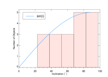
We assume that the brown dwarf rotates as a rigid sphere. However, this is not strictly true. The rotational period of Jupiter, as measured by magnetic fields originating in the core is , whereas the period measured using features rotating along the equator is , a difference of only minutes. Since rotational periods as measured from photometric variability in general have much larger uncertainties, the rigid body assumption is reasonable for our analysis. Thus, the equatorial rotation velocity, , is given by , where is the radius of the brown dwarf and is its rotation period. With our measured values of in hand, an assumption of radius and a measurement of the rotation period allow us to determine the angle of inclination, . Filippazzo et al. (2015) provide radius estimates from evolutionary models for 11/19 of our targets (starred in Table 5). We use reasonable radius estimates for the remaining field brown dwarfs. At field brown dwarf ages, the radii are independent of mass due to electron degeneracy (Burrows et al., 2001) and approach the radius of Jupiter. Therefore, the field brown dwarf targets are assumed to have a radius of . 2M1615+49 is the only young brown dwarf with no radius estimate. Since it has not been associated with any moving group (Faherty et al., 2016), we have no age constraint on this object. We assume a radius of , similar to other VL-G objects in the sample.
5 Results and Discussion
5.1 Effects of Inclination on Variability Amplitude
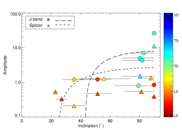
Figure 2 shows variability amplitude plotted against the angle of inclination. We note a number of interesting trends in the -band and Spitzer variable brown dwarfs.

Firstly, the highest amplitude -band variable objects are either L/T transition brown dwarfs or young, red brown dwarfs. The highest Spitzer and -band amplitudes are both for the L/T transition brown dwarf, 2M2139+02 . The Spitzer amplitudes for young brown dwarfs are slightly enhanced, but only relative to their own spectral type and not the entire Spitzer sample.
Secondly, while it is clear that each brown dwarf has its own intrinsic amplitude, the inclination angle affects the observed amplitude for both bands. Figure 2 shows that there are no mid-IR variability detections at inclination angles and no -band detections at inclination angles . Excluding the young objects, we find relatively low amplitudes at inclination angles . At inclinations close to we observe the highest variability amplitudes in both bands. This makes sense as the brown dwarf is nearly equator-on, allowing us to observe the full variability amplitude. An atmospheric feature observed on a low inclination object will appear smaller due to projection effects.
The -band amplitudes appear to be more affected by inclination than the Spitzer amplitudes. The highest -band variable objects appear at high inclinations, whereas a Spitzer brown dwarf viewed equator-on displays similar amplitudes to those observed at inclinations as low as . This may be explained by considering the pressures probed by each band. Biller et al. (2013), Buenzli et al. (2012) and Yang et al. (2016) determined the pressure level probed at optical depth as a function of wavelength for various models, finding that the -band probes a discrete range of pressures deep in the atmosphere. On the other hand, the Spitzer [m] band probes a broader range of pressures, that extend higher up in the photosphere. For the deep layers probed by the -band, the flux will be strongly attenuated for the low-inclination objects due to an increased path length through the atmosphere. The effect is not observed as strongly for Spitzer detections because more of the flux originates from near the top of the photosphere. Thus, we see -band amplitudes decrease strongly with decreasing inclination.

| -band | Spitzer [m] | |
|---|---|---|
We use a toy model to investigate the effects of inclination on the observed variability amplitude. Our model has two terms:
| (1) |
where is the observed amplitude and is the amplitude that would be observed if there were no atmospheric attenuation of the flux. is the factor by which the flux is attenuated as it passes through the atmosphere and is the atmospheric path length. The first term is a projection effect, which causes the observed area of a spot to decrease as the brown dwarf approaches lower inclinations. The second term represents the attenuation of the flux as it passes through the brown dwarf atmosphere. From the models discussed above, we expect that the -band path lengths are larger than the Spitzer path lengths. We fit the function for both bands, assuming that all objects have the same intrinsic amplitude. We consider only the field brown dwarfs since young objects will have very different atmospheric structures. The best fit functions are shown in Figure 5. The model fits the data reasonably well, displaying the earlier drop-off of the -band amplitudes compared to the Spitzer amplitudes due to a much larger -band term.
5.2 Relation between Period and Variability Amplitude
Figure 6 shows the variability amplitude plotted against rotation period for Spitzer and -band variable L, T and Y spectral type objects with published periods from the literature
The -band and Spitzer data display notably different period and variability amplitude properties. Ground-based -band detections have lower photometric precision, so in general -band detections are limited to larger amplitudes. It is clear that mid-IR variability is intrinsically lower than near-IR variability however, as high amplitude variability would certainly have been detected with Spitzer. Ground-based observations are only sensitive to shorter periods (hr), so the longer period variable brown dwarfs have been detected with Spitzer.
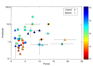
Figure 7 shows the variability amplitude plotted against rotation period for all -band variable objects with published periods (shown in Table 2). Measured periods are hr, since most -band detections are ground-based, and thus are sensitive to this range of periods. The highest amplitudes are L/T transition spectral types, as reported by Radigan et al. (2014). Additionally, for periods hr, there seems to be an overall increase in -band variability amplitude with longer periods.
We calculate the significance of this result by calculating Kendall’s using IDLs r_correlate.pro. Kendall’s is a nonparametric measure of correlation based on the relative ordering of the rank of each value in the dataset (Press et al., 1987). To define , we start with data points , and consider all pairs of data points. A pair is concordant if the relative ordering of the ranks of is the same as the relative ordering of the ranks of . A pair is discordant if the relative ordering of differs from the ordering of the ranks. When the relative ranks are the same, we call the pair an ”extra-” pair. Similarly, when relative ranks are the same, we get an ”extra-” pair. Kendall’s is then calculated using the equation:
| (2) |
| (3) |
Calculating the Kendall’s rank correlation coefficient and -value, we find that the relation between -band variability amplitude and rotational period (for periods hr) is significant with a -value . In contrast, including all periods, the correlation between period and amplitude is not significant, with a -value. This tentative correlation between variability amplitude and rotation period for periods hr may be explained by consideration of the Rhines length (Rhines, 1970). Organised jet features in the atmospheres of the giant Solar System planets generally scale in size with the Rhines length. This also represents the maximum attainable size that a coherent atmospheric structure can grow to before being destroyed by such zonal jets. The Rhines length is given by
| (4) |
where is the characteristic wind speed, is the radius, where is the period, and is the latitude of the atmospheric feature. Assuming that the wind speeds and latitudes are the same then . Thus we would expect the maximum atmospheric feature size to increase with longer rotational periods, explaining the increasing variability amplitude with period in Figure 7.
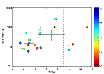
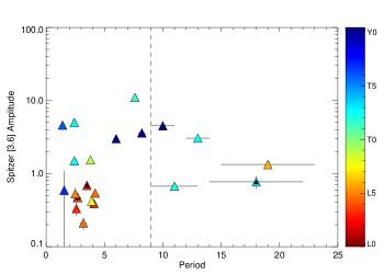
Figure 8 shows the Spitzer amplitudes plotted against rotation periods for all Spitzer variable objects with published periods (presented in Table 3). Spitzer observations are in general longer than ground-based -band observations (Metchev et al. (2015) employed hr observations for their Spitzer survey) and are thus sensitive to longer periods. Spitzer lightcurves have much higher photometric precision than ground-based studies and thus are also sensitive to lower amplitudes. However, clearly mid-IR variability is intrinsically lower than the near-IR variability. In contrast to the -band data, Kendall’s produces -value , thus we find no correlation between variability amplitude and rotation period in this case. At longer periods, the observed variability amplitudes appear to decrease, however the sparse number of data points prevents us from confirming this. The highest variability amplitudes in the mid-IR case are detected in the late T’s and early Y’s, in contrast to the -band, where high amplitudes are detected in L/T transition objects. Again, the young L-type objects may have slightly enhanced amplitudes when compared to field L-type brown dwarfs (Metchev et al., 2015).
5.3 Investigating Colour Anomalies of the Sample
We define the colour anomaly of each object as the median 2MASS colour subtracted from the colour of the object. Median colours for L0 - T6 objects were taken from Schmidt et al. (2010). For 2M0050, the T7 object, we calculated the median of all IR T7 objects from DwarfArchives.org (20 objects) and found the median T7 colour to be . This is a much higher error than those in Schmidt et al. (2010) and was thus left out of the analysis. With no measurement of Y dwarfs, it was not possible to include WISE0855, WISE1405 and WISE1738. Liu et al. (2016) provides linear relations between spectral type and absolute magnitude for VL-G and INT-G brown dwarfs, and these were used to calculate the median colours for the low-gravity sample.
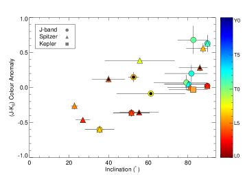
Figure 9 displays the colour anomaly of objects listed in Table 1 plotted against their inclinations. We note a correlation between the colour anomaly and inclination whereby objects viewed equator-on appear redder than objects viewed at lower inclinations.
Calculating the correlation coefficient and -value, we find that the relation between colour anomaly and inclination is statistically significant with a -value . Objects we observe to be redder than the median are equator-on, whereas objects appearing bluer than the median are closer to pole-on. This result could be interpreted by the idea first proposed by Kirkpatrick et al. (2010), that viewing angle determines the spectral appearance of a brown dwarf. This could occur if clouds are not homogenously distributed in latitude or if grain size and cloud thickness vary in latitude. Our results can be explained if thicker or large-grained clouds are situated at the equator, while thinner or small-grained clouds are situated at the poles.

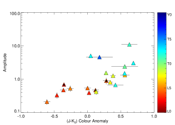
Figures 10 and 11 show the variability amplitude plotted against the colour anomaly for -band and Spitzer detections respectively. Both plots exhibit a consistent trend, whereby field objects that are redder than the median display higher -band and Spitzer variability amplitudes. The field objects with the highest observed variability amplitudes are those with the reddest colours of their spectral type. We find that this correlation is significant at the and levels for the -band and mid-IR detections respectively. This relation may be explained by consideration of viewing angle. If redder brown dwarfs are equator-on, and equator-on objects exhibit the highest amplitudes, then it follows that redder brown dwarfs should display the highest variability amplitudes. Similarly, bluer brown dwarfs are viewed close to pole-on, so the observed variability amplitude will be reduced due to the viewing angle.
6 Summary and Conclusions
In this paper we explored the effects of inclination angle on measured variability amplitudes and whether brown dwarfs display similar intrinsic amplitudes. We further went on to examine the relation between inclination angle and spectral appearance. We determined the inclination angle of 19 variable brown dwarfs using archival Keck data and estimates on radius. We analyse the full sample of L, T and Y spectral type brown dwarfs with published -band and Spitzer variability detections.
We conclude that brown dwarfs have different intrinsic amplitudes, dependent on properties such as spectral type, rotation period and surface gravity. In this paper we find evidence that the variability amplitude may increase with rotational period for periods hr. This result is significant at the level for band detections but is not significant for Spitzer detections. The inclination angle affects the observed amplitude due to a projection effect as well as atmospheric attenuation. Our toy model suggests that -band variability is more strongly affected by inclination when compared to Spitzer variability. This may be due to the -band probing deeper levels in the atmosphere. This results in the flux coming from these deeper levels being attenuated more due to increased path lengths at lower inclinations. All brown dwarfs with mid-IR variability detections are inclined at an angle . In the near-IR, we find that all brown dwarfs with -band variability detections are inclined at an angle .
We find a trend between the colour anomaly and inclination of our sample that is statistically significant at the level. Field objects viewed equator-on appear redder than the median for their spectral type, whereas objects viewed at lower inclinations appear bluer. This supports the idea that our viewing angle influences the spectral and photometric appearance of a brown dwarf. These results can be explained if thicker or large-grained clouds are situated at the equator, with thinner or small-grained clouds at the poles. We also find a strong correlation between colour anomaly and both mid-IR and -band variability, where redder objects have higher variability amplitudes. This again suggests that the spectral appearance of a brown dwarf is strongly affected by its inclination angle.
References
- Allard et al. (2012) Allard, F., Homeier, D., & Freytag, B. 2012, Philosophical Transactions of the Royal Society A: Mathematical, Physical and Engineering Sciences, 370, 2765
- Allers et al. (2016) Allers, K. N., Gallimore, J. F., Liu, M. C., & Dupuy, T. J. 2016, The Astrophysical Journal, 819, 133
- Allers & Liu (2013) Allers, K. N., & Liu, M. C. 2013, The Astrophysical Journal, 772, 79
- Apai et al. (2013) Apai, D., Radigan, J., Buenzli, E., et al. 2013, The Astrophysical Journal, 768, 121
- Artigau et al. (2009) Artigau, É., Bouchard, S., Doyon, R., & Lafrenière, D. 2009, The Astrophysical Journal, 701, 1534
- Bailer-Jones (2004) Bailer-Jones, C. A. L. 2004, Astronomy and Astrophysics, 419, 703
- Basri et al. (2000) Basri, G., Mohanty, S., Allard, F., et al. 2000, The Astrophysical Journal, 538, 363
- Berger et al. (2005) Berger, E., Rutledge, R. E., Reid, I. N., et al. 2005, The Astrophysical Journal, 627, 960
- Bertoldi et al. (1999) Bertoldi, F., Timmermann, R., Rosenthal, D., Drapatz, S., & Wright, C. M. 1999, Astronomy & Astrophysics, 346, 267
- Biller et al. (2013) Biller, B. A., Crossfield, I. J. M., Mancini, L., et al. 2013, The Astrophysical Journal, 778, L10
- Biller et al. (2015) Biller, B. A., Vos, J., Bonavita, M., et al. 2015, The Astrophysical Journal, 813, L23
- Blake et al. (2010) Blake, C. H., Charbonneau, D., & White, R. J. 2010, The Astrophysical Journal, 723, 684
- Buenzli et al. (2014) Buenzli, E., Apai, D., Radigan, J., Reid, I. N., & Flateau, D. 2014, The Astrophysical Journal, 782, 77
- Buenzli et al. (2015a) Buenzli, E., Marley, M. S., Apai, D., et al. 2015a, The Astrophysical Journal, 812, 163
- Buenzli et al. (2015b) Buenzli, E., Saumon, D., Marley, M. S., et al. 2015b, The Astrophysical Journal, 798, 127
- Buenzli et al. (2012) Buenzli, E., Apai, D., Morley, C. V., et al. 2012, The Astrophysical Journal, 760, L31
- Burrows et al. (2001) Burrows, A., Hubbard, W. B., Lunine, J. I., & Liebert, J. 2001, Reviews of Modern Physics, 73, 719
- Clarke et al. (2008) Clarke, F. J., Hodgkin, S. T., Oppenheimer, B. R., Robertson, J., & Haubois, X. 2008, Monthly Notices of the Royal Astronomical Society, 386, 2009
- Croll et al. (2016) Croll, B., Muirhead, P. S., Han, E., et al. 2016, arXiv:1609.03586
- Crossfield et al. (2014) Crossfield, I. J. M., Biller, B., Schlieder, J. E., et al. 2014, Nature, 505, 654
- Cruz et al. (2009) Cruz, K. L., Kirkpatrick, J. D., & Burgasser, A. J. 2009, The Astronomical Journal, 137, 3345
- Cushing et al. (2004) Cushing, M. C., Vacca, W. D., & Rayner, J. T. 2004, Publications of the Astronomical Society of the Pacific, 116, 362
- Cushing et al. (2006) Cushing, M. C., Roellig, T. L., Marley, M. S., et al. 2006, The Astrophysical Journal, 648, 614
- Cushing et al. (2016) Cushing, M. C., Hardegree-Ullman, K. K., Trucks, J. L., et al. 2016, The Astrophysical Journal, 823, 152
- Enoch et al. (2003) Enoch, M. L., Brown, M. E., & Burgasser, A. J. 2003, The Astronomical Journal, 126, 1006
- Esplin et al. (2016) Esplin, T. L., Luhman, K. L., Cushing, M. C., et al. 2016, The Astrophysical Journal, 832, 58
- Faherty et al. (2012) Faherty, J. K., Burgasser, A. J., Walter, F. M., et al. 2012, The Astrophysical Journal, 752, 56
- Faherty et al. (2016) Faherty, J. K., Riedel, A. R., Cruz, K. L., et al. 2016, The Astrophysical Journal Supplement Series, 225, 10
- Filippazzo et al. (2015) Filippazzo, J. C., Rice, E. L., Faherty, J., et al. 2015, The Astrophysical Journal, 810, 158
- Folkes et al. (2007) Folkes, S. L., Pinfield, D. J., Kendall, T. R., & Jones, H. R. A. 2007, Monthly Notices of the Royal Astronomical Society, 378, 901
- Gagné et al. (2015) Gagné, J., Faherty, J. K., Cruz, K. L., et al. 2015, The Astrophysical Journal Supplement Series, 219, 33
- Gillon et al. (2013) Gillon, M., Triaud, a. H. M. J., Jehin, E., et al. 2013, Astronomy & Astrophysics, 555, L5
- Girardin et al. (2013) Girardin, F., Artigau, É., & Doyon, R. 2013, The Astrophysical Journal, 767, 61
- Gizis et al. (2015) Gizis, J. E., Allers, K. N., Liu, M. C., et al. 2015, The Astrophysical Journal, 799, 203
- Gizis et al. (2013) Gizis, J. E., Burgasser, A. J., Berger, E., et al. 2013, The Astrophysical Journal, 779, 172
- Gizis et al. (2012) Gizis, J. E., Faherty, J. K., Liu, M. C., et al. 2012, The Astronomical Journal, 144, 94
- Harding et al. (2013) Harding, L. K., Hallinan, G., Boyle, R. P., et al. 2013, The Astrophysical Journal, 779, 101
- Heinze et al. (2014) Heinze, A. N., Metchev, S., & Kellogg, K. 2014, The Astrophysical Journal, 767, 173
- Jackson & Jeffries (2010) Jackson, R. J., & Jeffries, R. D. 2010, Monthly Notices of the Royal Astronomical Society, 402, 1380
- Karalidi et al. (2016) Karalidi, T., Apai, D., Marley, M. S., & Buenzli, E. 2016, The Astrophysical Journal, 825, 90
- Kirkpatrick et al. (2010) Kirkpatrick, J. D., Looper, D. L., Burgasser, A. J., et al. 2010, The Astrophysical Journal Supplement Series, 190, 100
- Kostov & Apai (2013) Kostov, V., & Apai, D. 2013, The Astrophysical Journal, 762, 47
- Leggett et al. (2016) Leggett, S. K., Cushing, M. C., Hardegree-Ullman, K. K., et al. 2016, The Astrophysical Journal, 830, 141
- Lew et al. (2016) Lew, B. W. P., Apai, D., Zhou, Y., et al. 2016, The Astrophysical Journal, 829, L32
- Liu et al. (2016) Liu, M. C., Dupuy, T. J., & Allers, K. N. 2016, The Astrophysical Journal, 833, 96
- Liu et al. (2013) Liu, M. C., Magnier, E. A., Deacon, N. R., et al. 2013, The Astrophysical Journal, 777, L20
- Looper et al. (2010) Looper, D. L., Mohanty, S., Bochanski, J. J., et al. 2010, The Astrophysical Journal, 714, 45
- Luhman (2014) Luhman, K. L. 2014, The Astrophysical Journal, 786, L18
- Madhusudhan et al. (2011) Madhusudhan, N., Burrows, A., & Currie, T. 2011, The Astrophysical Journal, 737, 34
- Marocco et al. (2014) Marocco, F., Day-Jones, A. C., Lucas, P. W., et al. 2014, Monthly Notices of the Royal Astronomical Society, 439, 372
- Metchev et al. (2013) Metchev, S., Apai, D., Radigan, J., et al. 2013, Astronomische Nachrichten, 334, 40
- Metchev et al. (2015) Metchev, S. A., Heinze, A., Apai, D., et al. 2015, The Astrophysical Journal, 799, 154
- Press et al. (1987) Press, W., Teukolsky, S., Vetterling, W., et al. 1987, 501, arXiv:arXiv:1011.1669v3
- Radigan (2014) Radigan, J. 2014, The Astrophysical Journal, 797, 120
- Radigan et al. (2012) Radigan, J., Jayawardhana, R., Lafrenière, D., et al. 2012, The Astrophysical Journal, 750, 105
- Radigan et al. (2014) Radigan, J., Lafrenière, D., Jayawardhana, R., & Artigau, E. 2014, The Astrophysical Journal, 793, 75
- Reiners & Basri (2008) Reiners, A., & Basri, G. 2008, The Astrophysical Journal, 684, 1390
- Rhines (1970) Rhines, P. 1970, Geophysical Fluid Dynamics, 1, 273
- Schmidt et al. (2010) Schmidt, S. J., West, A. A., Hawley, S. L., & Pineda, J. S. 2010, The Astronomical Journal, 139, 1808
- Ter Braak & Vrugt (2008) Ter Braak, C. J. F., & Vrugt, J. A. 2008, Statistics and Computing, 18, 435
- Walkowicz et al. (2013) Walkowicz, L. M., Basri, G., & Valenti, J. a. 2013, The Astrophysical Journal Supplement Series, 205, 17
- Wilson et al. (2014) Wilson, P. A., Rajan, A., & Patience, J. 2014, Astronomy & Astrophysics, 566, A111
- Yang et al. (2016) Yang, H., Apai, D., Marley, M. S., et al. 2016, The Astrophysical Journal, 826, 8
- Zhou et al. (2016) Zhou, Y., Apai, D., Schneider, G. H., Marley, M. S., & Showman, A. P. 2016, The Astrophysical Journal, 818, 176