ExoMol Line List XXI: Nitric Oxide (NO)

Abstract

Line lists for the X ${}^{2}\Pi$ electronic ground state for the parent isotopologue of nitric oxide (¹⁴N¹⁶O) and five other major isotopologues (¹⁴N¹⁷O, ¹⁴N¹⁸O, ¹⁵N¹⁶O, ¹⁵N¹⁷O and ¹⁵N¹⁸O) are presented. The line lists are constructed using empirical energy levels (and line positions) and high-level ab inito intensities. The energy levels were obtained using a combination of two approaches, from an effective Hamiltonian and from solving the rovibronic Schrödinger equation variationally. The effective hamiltonian model was obtained through a fit to the experimental line positions of NO available in the literature for all six isotopologues using the programs SPFIT and SPCAT. The variational model was built through a least squares fit of the ab inito potential and spin-orbit curves to the experimentally derived energies and experimental line positions of the main isotopologue only using the Duo program. The ab inito potential energy, spin-orbit and dipole moment curves (PEC, SOC and DMC) are computed using high-level ab inito methods and the MARVEL method is used to obtain energies of NO from experimental transition frequencies. The line lists are constructed for each isotopologue based on the use of the most accurate energy levels and the ab inito DMC. Each line list covers a wavenumber range from 0 - 40,000 cm^-1with approximately 22,000 rovibronic states and 2.3 – 2.6 million transitions extending to $J_{max}=184.5$ and $\varv_{max}=51$. Partition functions are also calculated up to a temperature of 5000 K. The calculated absorption line intensities at 296 K using these line lists show excellent agreement with those included in the HITRAN and HITEMP databases. The computed NO line lists are the most comprehensive to date, covering a wider wavenumber and temperature range compared to both the HITRAN and HITEMP databases. These line lists are also more accurate than those used in HITEMP. The full line lists are available from the CDS http://cdsarc.u-strasbg.fr and ExoMol www.exomol.com databases; data will also be available from CDMS www.cdms.de.

1 Introduction

NO has been detected in several interstellar environments ranging from a starburst galaxy (Martin et al., 2003, 2006) to dark clouds (McGonagle et al., 1990) and numerous star-forming regions (Ziurys et al., 1991). It is also present in the atmospheres of Earth, Mars and Venus, and its emission is a major source of nightglow in these three planets (Cox et al., 2008; Eastes et al., 1992; Royer et al., 2010). The presence of NO in Earth’s atmosphere has a significant impact on depletion of the ozone layer (Barry & Chorley, 2010; Wayne, 2000) and originates from the reaction of N₂O with O(¹D) in the stratosphere. In the troposphere the major sources of NO are of anthropogenic origin as it is produced during fuel combustion at temperatures of $\sim$2300 K (Flagan & Seinfeld, 1988) and through soil cultivation. Because NO (and NO₂) catalyze the production of tropospheric ozone, it is important to try to reduce NO emissions (amongst other air pollutants). Whilst NO has not yet been detected in an exoplanet atmosphere, it is likely present in its gaseous form in terrestrial-type atmospheres, for example produced during a storm soon after a lightning shock (Ardaseva et al., 2017).

There are currently two commonly used databases which contain line lists for NO in its electronic ground state: HITRAN (Rothman et al., 2013) which covers ¹⁴N¹⁶O, ¹⁴N¹⁸O and ¹⁵N¹⁶O, and is designed for use near room temperature, and HITEMP (Rothman et al., 2010) which allows the spectrum of ¹⁴N¹⁶O to be modelled up to 4000 K. HITRAN and HITEMP databases contain 103,702 and 115,610 transitions, respectively, with ${J_{max}=125.5}$ and ${v_{max}=14}$.

The aim of this work is to produce a line list for the X ${}^{2}\Pi$ electronic ground state of nitric oxide for its parent isotopologue (¹⁴N¹⁶O, hereafter NO), and five major isotopologues (¹⁴N¹⁷O, ¹⁴N¹⁸O, ¹⁵N¹⁶O, ¹⁵N¹⁷O and ¹⁵N¹⁸O). Using a combination of high level ab initio methods, accurate fitting to a comprehensive set of experimental data and variational modeling, six line lists for these species were constructed. These line lists consist of rovibronic energy levels, with all of the associated quantum numbers, transition wavenumbers and Einstein-A coefficients. The computed line lists form part of the ExoMol database (Tennyson et al., 2016c) which aims to provide a comprehensive set of high-temperature line lists for molecules that may be present in hot atmospheres such as those of exoplanets, planetary disks, brown dwarfs and cool stars (Tennyson & Yurchenko, 2012). Many ExoMol line lists have already been used in the characterisation and modelling of brown dwarf and exoplanet atmospheres (Tinetti et al., 2007; Cushing et al., 2011; Yurchenko et al., 2014; Molliere et al., 2015; Morley et al., 2015; Barman et al., 2015; Beaulieu et al., 2011; Canty et al., 2015; Morley et al., 2014; Tsiaras et al., 2016).

The ExoMol database also contains line lists for numerous diatomic molecules generated by the ExoMol project: AlO (Patrascu et al., 2015), BeH, MgH and CaH (Yadin et al., 2012), SiO (Barton et al., 2013), CaO (Yurchenko et al., 2016b), CS (Paulose et al., 2015), NaCl and KCl (Barton et al., 2014), NaH (Rivlin et al., 2015), PN (Yorke et al., 2014), ScH (Lodi et al., 2015) and VO (McKemmish et al., 2016). Line lists available from other sources include: CrH (Burrows et al., 2002), FeH (Dulick et al., 2003), TiH (Burrows et al., 2005), CaH (Li et al., 2012), MgH (GharibNezhad et al., 2013), CN (Brooke et al., 2014), OH (Brooke et al., 2016), NH (Brooke et al., 2015), and ZrS (Farhat, 2017).

These line lists often include many of the abundant isotopologues and greatly extend the calculated range of ${J}$ and ${v}$ in comparison to the HITRAN and HITEMP databases. High-temperature line lists are useful in the characterisation of brown dwarfs (Yurchenko et al., 2014), which have atmospheric temperatures ranging from 500-3000 K (Perryman, 2014). The hot NO line lists produced from this work can be used directly in characterization of the spectra of such objects, as well as in atmospheric models (de Vera & Seckbach, 2013).

The remainder of this paper is divided into several sections. Section 2 outlines the methods used in the calculation of energy levels and production of the line lists, whilst Section 3 presents the results of this work - mainly the NO line list, the calculated partition function and radiative lifetimes. Absorption line intensities and cross-sections are also shown. Finally, Section 4 discusses the implications of this work, and how it will be significant to the astrophysical community.

2 Methods

2.1 Experimental Data

2.1.1 Extraction of Experimental Data

Transition frequencies for the X ${}^{2}\Pi$ electronic ground state of NO were collected from selected experimental papers, see Table 1, along with any given quantum numbers and uncertainties for all six isotopologues. This table also indicates whether a dataset was used for the MARVEL analysis (M), SPFIT calculations (S) or both (see below). We used the MARVEL program (Measured Active Rotational-Vibrational Energy Levels) (Furtenbacher et al., 2007; Furtenbacher & Császár, 2012a) to derive energy levels of the main isotopologue ¹⁴N¹⁶O based on the experimental transition data available in the literature. These data were then utilized to refine our ab initio model using the Duo program (Yurchenko et al., 2016a). The more extensive SPFIT set of experimental frequencies covering all six isotopologues was used to obtain NO spectroscopic constants in a global fit using the effective Hamiltonian programs SPFIT and SPCAT (Pickett, 1991).

Table 1: Experimental papers on NO spectra.

Source	States	Isotopologue; Methodsa	M/Sb	Range in $J$ and/or $\varv$
64James	James (1964)	NO; IR	M	$J=0.5-21.5$
64JaThxx	James & Thibault (1964)	NO; IR	M	$J=1.5-21.5$
70Neumann	Neumann (1970)	NO; RF, $\mu$	S	$J=0.5-7.5$, $\varv=0$
72MeDyxx	Meerts & Dymanus (1972)	NO, 15NO; IR	S	$J=0.5-8.5$, $\varv=0$
76Meerts	Meerts (1976)	NO; RF	S	$J=4.5-5.5$, $\varv=0$
77DaJoMc	Dale et al. (1977)	NO; IR-RF DR	S	$J=4.5-5.5$, $\varv=0$, 1
78AmBaGu	Amiot et al. (1978)	NO; FTIR	S	$J=0.5-40.5$, $\varv=1-0$, $2-1$
78HeLeCa	Henry et al. (1978)	NO; FTIR	S	$J=0.5-28.5$, $\varv=3-0$
79AmGuxx	Amiot & Guelachvili (1979)	15NO, 15N17O, 15N18O; FTIR	S	$J=0.5-41.5$, $\varv=1-0$, $2-1$
79PiCoWa	Pickett et al. (1979)	NO; mmW, smmW	S	$J=0.5-4.5$, $\varv=0$
80AmVexx	Amiot & Verges (1980)	NO; Emi, FTIR 2900$-$3810 cm-1.	M,S	$J=0.5-57.5$, $\varv=0-15$, $\Delta v=2$
80TeHeCa	Teffo et al. (1980)	15NO, 15N18O; FTIR	S	$J=0.5-32.5$, $\varv=1-0$, $2-0$, $3-0$
80VaMeDy	Van den Heuvel et al. (1980)	NO; TuFIR	M	$J=7.5-10.5$
81LoMcVe	Lowe et al. (1981)	NO; IR-RF DR	S	$J=12.5-20.5$, $\varv=0$, 1
82Amiot	Amiot (1982)	NO; Emi, FTIR, 3800$-$5000 cm-1	M,S	$J=0.5-59.5$, $\varv=7-22$, $\Delta\varv=3$
86HiWeMa	Hinz et al. (1986)	NO; heterodyne IR	S	$J=1.5-32.5$, $\varv=1-0$
91SaYaWi	Saleck et al. (1991)	15NO, N18Oc; mmW, smmW	S	$J=0.5-4.5$, $\varv=0$
92RaFrMi	Rawlins et al. (1992)	NO; IR ChLumi, 2.7$-$3.3${\mu}$m	M	5.2$-$6.8 $\mu$m $\varv^{\prime}=2-3$
94DaMaCo	Dana et al. (1994)	NO; FTIR	M,S	$J=2.5-24.5$, $\varv=2-1$
94MaDaCo	Mandin et al. (1994)	NO; FTIR	M	$J=1.5-20.5$, $\varv=1-0$
94SaLiDo	Saleck et al. (1994)	N17O and 15N18O; mmW	S	$J=0.5-2.5$, $\varv=0$
94SpChGi	Spencer et al. (1994)	NO; FTIR 1780$-$1960 cm-1	M,S	$J=0.5-25.5$, $\varv=1-0$
95CoDaMa	Coudert et al. (1995)	NO; FTIRd 1730$-$1990 cm-1	M,S	$J=0.5-41.5$, $\varv=1-0$
96SaMeWa	Saupe et al. (1996)	NO; heterodyne IR	S	$J=8.5-18.5$, $\varv=1-0$
97DaDoKe	Danielak et al. (1997)	O2/N2; Ebert spectrograph	M	$\varv=0-7$
97MaDaRe	Mandin et al. (1997)	NO; FTIR, 3600$-$3800 cm-1	M,S	$J=2.5-32.5$, $\varv=2-0$
98MaDaRe	Mandin et al. (1998)	NO; FTIR, 3600$-$3720 cm-1	M	$J=2.5-17.5$, $\varv=3-1$
99VaStEv	Varberg et al. (1999)	NO; TuFIR, 11$-$157 cm-1	M	$J=2.5-38.5$
99VaStEv	Varberg et al. (1999)	NO; 15NO; TuFIR, 11$-$157 cm-1	S	$J=2.5-38.5$, $\varv=0$
01LiGuLi	Liu et al. (2001)	NO; IR LMR, $\mu$	S	$J=1.5-2.5$, $\varv=1-0$
06LeChOg	Lee et al. (2006)	NO; FTIR	M	$J=0.5-30.5$, $\varv^{\prime}=2-6$
06BoMcOs	Bood et al. (2006)	NO; NICE-OHMS	M	$J=2.5-16.5$, $\varv=7-0$
15MuKoTa	Müller et al. (2015)	N18O; TuFIR, 33$-$159 cm-1	S	$J=3.5-26.5$, $\varv=0$

^a Unlabelled atoms refer to ¹⁴N or ¹⁶O. Abbreviations: IR (infrared), FT (Fourier transform), ChLumi (chemiluminescence), Emi (emission), DR (double resonance), $\mu$ (dipole moment), RF (radio frequency), MW (microwave), mmW (millimetre wave), smmW (sub-millimetre wave), TuFIR (tunable far-infrared), LMR (laser magnetic resonance).
^b Used for MARVEL (M) and/or SPFIT (S);
^c NO FIR data not used. ^d Wavenumber recalibration proposed, see section 2.4.

2.1.2 MARVEL

MARVEL is an algorithm which calculates rovibronic energy levels from a given set of experimental transitions. The online version of the program was used, as the output files are formatted to be more user-friendly. An extraction from our MARVEL input-file is given in Table 2.

The experimental literature was chosen to ensure that a full range of transitions was included whilst minimising duplication of data. Although the default MARVEL procedure utilises all of the data included in the input file (Furtenbacher & Császár, 2012b), if there happens to be any data overlap between papers, only the most accurate (and in general the most recent) data are considered. Only transitions within the ground electronic state were considered for our MARVEL analysis.

Pure rotational transition frequencies were taken from Van den Heuvel et al. (1980), Lovas & Tiemann (1974) and Varberg et al. (1999), whilst transitions between the two $\Lambda$-doublet states (X ${}^{2}\Pi_{\nicefrac{{1}}{{2}}}$ and X ${}^{2}\Pi_{\nicefrac{{3}}{{2}}}$) were taken from Mandin et al. (1994). Rovibrational transitions, extending up to $\Delta\varv=3$, $\varv^{\prime}=22$ and $J^{\prime}=58.5$, were taken from the work by Amiot (1982), Amiot & Verges (1980), Bood et al. (2006), Coudert et al. (1995), Lee et al. (2006), Mandin et al. (1997), Mandin et al. (1998) and Spencer et al. (1994).

It should be noted that the spectroscopic notation is not consistent in the literature, thus making it necessary to generate a consistent set of quantum numbers for each transition. For many of the rovibrational papers, the $P$, $Q$ and $R$ labels were used to derive $J^{\prime}$ if $J^{\prime}$ and $J^{\prime\prime}$ had not already been specified. In the case of Amiot (1982) and Amiot & Verges (1980), the projection of the total angular momentum ($\Omega$) was determined by assigning transitions labelled $P_{1}$ and $R_{1}$ to a value of $\Omega^{\prime\prime}=\frac{1}{2}$ and those labelled $P_{2}$ and $R_{2}$ to the corresponding $\Omega^{\prime\prime}=\frac{3}{2}$. Rotationless parities of lower levels were given in terms of $e$ and $f$ by Coudert et al. (1995), Mandin et al. (1994), Mandin et al. (1997) and Spencer et al. (1994). For papers that did not specify parity, this was resolved by duplicating the dataset and assigning the parity $e$ to one set and the parity $f$ to the other. Hyperfine splitting was also resolved, albeit only in a few pure rotational papers (Van den Heuvel et al. (1980), Lovas & Tiemann (1974) and Varberg et al. (1999)), however at this stage of our analysis the hyperfine splitting was ignored. For rovibrational transitions sharing the same quantum numbers ($\Omega$’, $\Omega^{\prime\prime}$, $J^{\prime}$, $J^{\prime\prime}$ and $e/f$) but different frequency, an average of the two frequencies was taken and the frequency uncertainty was propagated. In lieu of any specified transition frequency uncertainties, estimates were made based upon the precision with which frequencies were quoted.

Table 2: MARVEL format of the experimental data: extract from the MARVEL input file.

Wavenumber (cm^-1) Uncertainty (cm^-1) $J^{\prime}$ Parity’ $\varv^{\prime}$ $\Omega$’ $J^{\prime\prime}$ Parity” $\varv^{\prime\prime}$ $\Omega^{\prime\prime}$ Reference 1985.3307 0.005 42.5 - 1 0.5 41.5 + 0 0.5 95CoDaMa80 1806.6561 0.005 17.5 + 1 1.5 18.5 - 0 1.5 95CoDaMa81 1806.6561 0.005 17.5 - 1 1.5 18.5 + 0 1.5 95CoDaMa82 1802.5924 0.005 18.5 + 1 1.5 19.5 - 0 1.5 95CoDaMa83 1802.5924 0.005 18.5 - 1 1.5 19.5 + 0 1.5 95CoDaMa84 1798.4950 0.005 19.5 + 1 1.5 20.5 - 0 1.5 95CoDaMa85 1798.4950 0.005 19.5 - 1 1.5 20.5 + 0 1.5 95CoDaMa86 1794.3687 0.005 20.5 + 1 1.5 21.5 - 0 1.5 95CoDaMa87 1794.3687 0.005 20.5 - 1 1.5 21.5 + 0 1.5 95CoDaMa88 1790.2060 0.005 21.5 + 1 1.5 22.5 - 0 1.5 95CoDaMa89 1790.2060 0.005 21.5 - 1 1.5 22.5 + 0 1.5 95CoDaMa90 1786.0180 0.005 22.5 + 1 1.5 23.5 - 0 1.5 95CoDaMa91

The $e/f$ parity of the lower energy states were converted to +/- total parity using the following standard relations:

$$\begin{array}[]{cl}e:&{\rm parity}=(-1)^{J-\frac{1}{2}}\\ f:&{\rm parity}=(-1)^{J+\frac{1}{2}},\end{array}$$

where $-1$ and $+1$ corresponds an odd (–) parity and even parity (+), respectively. The + $\leftrightarrow$ – selection rule was used to determine the parity of the upper state. For each transition, the electronic state and the projection of the electronic angular $\Lambda$ remained unchanged as only ro-vibrational transitions within the X ${}^{2}\Pi$ electronic ground state were considered in this work.

The quoted uncertainty of some transition frequencies were found to be either too large or too small. In these cases, the uncertainty value was adjusted to agree with the MARVEL-suggested uncertainty. After some trial and error, a clean run in MARVEL with no errors was achieved yielding a network of 4106 energy levels for NO with $\varv_{\rm max}=22$, $J_{\rm max}=58.5$ and a term value maximum of 36,200 cm^-1. The MARVEL energies obtained and the input file containing experimental transition frequencies are given as supplementary material to this paper.

The MARVEL procedure has previously been used to treat two other open shell diatomics of astronomical importance: C₂ (Furtenbacher et al., 2016) and TiO (McKemmish et al., 2017). The treatment of a single, albeit ${}^{2}\Pi$, state here proved to be much simpler than either of those studies, which included a large number of electronic transitions.

2.2 Ab Initio calculations

The ab initio potential energy curve (PEC), spin-orbit curve (SOC) and dipole moment curve (DMC) for the X ${}^{2}\Pi$ electronic ground state of NO were calculated using MOLPRO (Werner et al., 2012). An active space representation of (7,2,2,0) was chosen and an internally contracted multireference configuration interaction (icMRCI) method was used with Dunning type basis sets (Peterson & Dunning, 2002). A quadruple-$\zeta$ aug-cc-pwCVQZ-DK basis set was used to calculate the PEC and SOC, whereas the DMC was calculated using a quintuple-$\zeta$ aug-cc-pwCV5Z-DK basis set. The range of 0.6 – 10.0 Å was used with a dense grid of 350 geometries. Relativistic corrections for the DMC were also evaluated based on the Douglas-Kroll-Hess (DKH) Hamiltonian which included core correlation. The ab initio PEC and SOC are shown in Fig. 1.

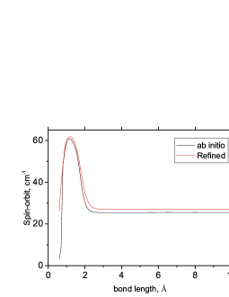
Figure 1: Ab initio and Duo refined PECs (upper display) and SOCs (lower display). The middle display shows the difference between the ab initio and refined PECs.

A quadruple-$\zeta$ basis set was considered sufficient for the PEC and SOC as these ab initio curves were fitted to the experimental data using Duo. A more accurate level of theory MRCI/aug-cc-pwCV5Z-DK Werner & Knowles (1988); Balabanov & Peterson (2005, 2006) with the relativistic corrections based on the Douglas-Kroll-Hess hamiltonian and core-correlated was used for the DMC as implemented in MOLPRO Werner et al. (2012). The DMC was calculated using the energy-derivative method (Lodi & Tennyson, 2010) which calculates the dipole moment as a derivative of the electronic energy $E(F)$ with respect to an external electric field $F$ ($F=0.0005$ a.u. in this case) using finite differences. A dipole moment of ${\mu_{e}}=0.166$ D at an equilibrium internuclear distance $r_{\rm e}=1.15~{}\AA\$ was obtained. Neumann (1970) reported an experimental value for $\mu_{0}=0.15782~{}(2)$ D, and Liu et al. (2001) determined $\mu_{0}=0.1595~{}(15)$ D and $\mu_{1}=0.1425~{}(16)$ D. Our value agrees very well with the value 0.1680 (19) D for both $\mu_{0}$ and $\mu_{1}$ obtained using data from Liu et al. (2001). The ab initio DMC is shown in Fig. 2.

Figure 2: Ab initio MRCI/aug-cc-pwCV5Z-DK dipole moment curve of NO.

2.3 Duo: Fitting

Duo is a program designed to solve a coupled Schrödinger equation for the motion of nuclei of a given diatomic molecule characterized by an arbitrary set of electronic states (Yurchenko et al., 2016a). Based on Hund’s case (a), Duo is capable of both refining potential energy curves (by fitting data to experimental energies or transition frequencies) and producing line lists. An extensive discussion of this method to calculate the direct solution of the vibronic Schrödinger equation has been given in a recent topical review (Tennyson et al., 2016b).

For this study, the range of computed $J$ levels was chosen to roughly correspond to all bound states of the system, i.e. to all states below $D_{0}$ ($J$ = 0.5 – 184.5). The vibrational basis set was specified to have $\varv_{\rm max}$ = 51, which also corresponds to the maximal number of vibrational states (taken at $J=0$). The sinc DVR method (Yurchenko et al., 2016a) defined on a grid of 701 points evenly distributed between 0.6 – 4.0 Å was used in integrations. The sinc DVR allows one to reduce the number of points with no significant lost of accuracy. For example, all energies obtained with this grid coincide with the energies obtained using a larger grid of 3001 points to better than $10^{-6}$ cm^-1.

The PEC and SOC were defined using the Extended Morse Oscillator (EMO) potential (Lee et al., 1999) given by

$$V(r)=V_{\rm e}+D_{\rm e}\Bigg{[}1-\exp\Bigg{(}-\beta_{\rm EMO}(r)(r-r_{\rm e})\Bigg{)}\Bigg{]}^{2},$$ (1)

where $D_{\rm e}$ is the dissociation energy; $N$ is the expansion order parameter; $r_{\rm e}$ is the equilibrium internuclear bond distance; $\beta_{\rm EMO}$ is the distance dependent exponent coefficient, defined as

$$\beta_{\rm EMO}(r)=\sum\limits_{i=0}^{N}B_{i}y_{p}(r)^{i}$$ (2)

and ${y_{p}}$ is the S̆urkus variable (Šurkus et al., 1984) given by

$$y_{p}(r)=\frac{r^{p}-r^{p}_{\rm e}}{r^{p}+r^{p}_{\rm e}}$$ (3)

with $p$ as a parameter. The EMO form is our common choice for representing PECs of diatomics (Patrascu et al., 2015; Yurchenko et al., 2016b; Lodi et al., 2015; McKemmish et al., 2016). It guarantees the correct dissociation limit and also allows extra flexibility in the degree of the polynomial around a reference position $R_{\rm ref}$, which was defined as the equilibrium internuclear separation ($r_{\rm e}$) in this case. It is also very robust in the fit. The disadvantage of EMO is that it does not correctly describe the dissociative part of the curve. As we show below, this drawback does not have a significant impact on our line lists.

A reasonable alternative to EMO is the Morse/long-range (MLR) potential representation (Roy & Henderson, 2007; Roy et al., 2009; Le Roy et al., 2011), which guarantees a physically correct, multipole-type representation of the PEC as inverse powers of $r$ for $r\to\infty$. The disadvantage of MLR (at least according to our experience) is that it less robust than EMO in refinements, requiring very careful determination of the switching and damping functions (see, for example, Le Roy et al. (2011)). Furthermore Lodi et al. (2008) showed that for strongly bound systems the multipole-type expansion is unnecessary and “possibly harmful”, except for very large values of $r$ ($>10a_{0}$ in case of H₂), which is certainly not the case here. Therefore our choice was to use EMO. As shown below, our line list is truncated at 40,000 cm^-1, and thus does not come very close to the long-range of the NO PEC.

The ab initio PEC and SOC were fitted to the experimental line positions of ¹⁴N¹⁶O available in the literature combined with the experimentally derived energies generated by MARVEL. From our experience a combination of line positions and energy levels provides a more stable fit. A total of nine potential expansion parameters ($B_{0},\ldots,B_{8}$) was required in order to obtain an optimal fit. The addition of any more parameters did not improve the fit significantly. In the case of the SOC refinement, an inverted EMO potential is used (Fig. 1) and required only four expansion parameters ($B_{0},\ldots,B_{3}$) to achieve a satisfactory fit.

The experimental value $D_{0}$ is 52,400 $\pm 10$ cm^-1 estimated by Callear & Pilling (1970) using fluorescence experiments and from Ackermann & Miescher (1969). We decided to refine the dissociation energy ($D_{\rm e}$) and not to constrain it to the experimental value of Callear & Pilling (1970). Varying $D_{\rm e}$ parameter led to a more compact form of $\beta_{\rm EMO}(r)$ with $N=6$ instead $N=8$: less expansion parameters usually means a more stable extrapolation. In fact Devivie & Peyerimhoff (1988) noted in their MRD-CI study the change of the dominant character of the reference electronic configurations in NO PEC at about 3 and 5 bohr ( 29100 cm^-1and $~{}51800$ cm^-1 respectively), when approaching the dissociation N(${}^{4}S$) + O(${}^{3}P$) (from $\pi^{4}\pi^{*}$ to $\sigma\pi^{3}\pi_{x}^{*}\pi_{y}^{*}\sigma^{*}$). That is, it is difficult to obtain a reliable connection between the equilibrium and experimental $D_{0}$ without sampling the highly vibrationally excited states ($v>48$) experimentally in the fit. Due to the lack of these data and also that the dissociation region was not our priority, we decided to adopt the refined $D_{\rm e}$ value. Our final SO-free $D_{0}$ is 51608 (6.400 eV), which is of  800 cm^-1 away from the experiment. This should not affect the quality of our line list for the selected temperatures. The $D_{0}$ value is estimated using the refined value of $D_{\rm e}=52495.3$ cm^-1  (see Table 3) and the lowest energy relative to the PEC minimum $V_{\rm e}$ of $E_{J=0.5,\Omega=0.5,v=0}=887.100$ cm^-1. Polak & Fiser (2004) reported a high-level ab initio level $D_{\rm e}$ value (MR-ACPF(TQ)) of 51,140 cm^-1 (6.340 eV).

The resulting EMO parameters, including the reference (equilibrium) bond length ($r_{\rm e}$), dissociation energy ($D_{\rm e}$), expansion ($B_{n}$) and $p$ parameters are listed in Table 3. The ab initio potential energy and spin-orbit curves are compared to the refined curves from Duo in Fig. 1. The ab initio PEC is in good agreement with the refined PEC, despite the very aggressive fit applied with a large number of $B_{n}$ expansion parameters. The ab initio spin-orbit curve was changed substantially by fitting, although the overall shape of the ab initio SOC is maintained in the refined curve, which is reassuring.

To account for spin-rotation and $\Lambda$-doubling effects, a polynomial expansion based on the S̆urkus-variables was used:

$$V(r)=D_{\rm e}+(1-y^{eq}_{p})\sum\limits^{N}_{n\geq 0}A_{n}(y^{eq}_{p})^{i}$$ (4)

where $N$ and $p$ are parameters, and $A_{n}$ is an expansion parameter refined in Duo. Both the spin-rotation $\gamma(r)$ and $\Lambda$-doubling $[p+2q](x)$ (see, for example Brown & Merer (1979)) functions were fitted with two expansion parameters $A_{0}$ and $A_{1}$. These are given in Table 4 along with the $p$ and $N$ parameters. Varying the Born-Oppenheimer breakdown corrections (Le Roy & Huang, 2002) did not lead to a significant improvement, at least within the root-means squares achieved, and therefore were excluded from the fit. In fact the effective interaction with other electronic states was partly recovered by inclusion of the Lambda-doubling and spin-rotation effective functions.

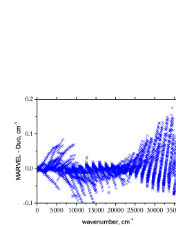
Figure 3: Obs. - Calc. residuals of the final energy level fit, where the calculated values are the refined energies calculated by Duo and the observed values are the MARVEL energies and experimental frequencies.

Table 3: Parameters for the refined potential energy and spin-orbit curves, modelled using the Extended Morse Oscillator function, see Eq. (1).

Parameter	Potential Energy Curve	Spin Orbit Curve
$V_{\rm e}$ (cm-1)	0	61.79345640612
$D_{\rm e}$ (cm-1)	52495.307750971	26.97757067068
$r_{\rm e}$ (Å)	1.1507863151853	1.2
${p}$	4	4
${N_{l}}^{a}$	2	1
${N_{r}}^{a}$	8	4
${B_{0}}$	2.76573276212320	1.3782871519399
${B_{1}}$	0.17739962868001	0.2416353146388
${B_{2}}$	0.12996658564591	-2.4682888462767
${B_{3}}$	1.81747768030430	5.5161066471770
${B_{4}}$	-9.76786082439320
${B_{5}}$	32.55261795679300
${B_{6}}$	-57.64002246220800
${B_{7}}$	55.24637383442700
${B_{8}}$	-21.23174396925500

^a The upper bound parameter $N$ in Eq. (2) is defined as $N=N_{l}$ for $r\leq r_{\rm e}$ and $N=N_{r}$ for $r>r_{\rm e}$.

Table 4: Parameters for the refined spin-rotation and $\Lambda$-doubling expressions, modelled using the S̆urkus polynomial expansion, see Eq. (4).

Parameter	Spin-Rotation	$\Lambda$-$[p+2q]$
$r_{\rm e}(\AA)$	1.1507863151853	1.1507863151853
${p}$	4	3
${N}$	1	1
${A_{0}}$	-0.0047317777443454	0.0061357379499906
${A_{1}}$	-0.0175102918408170	-0.0057848693802985

Experimental transition frequencies were introduced to the data set at the final stage of the fitting procedure in order to generate the most accurate set of parameters possible. The final residuals from fitting the Duo energy levels are plotted in Fig. 3. Notably, the largest residuals originate from energy levels with high $J$ and $\varv$, in particular $J>35.5$ and $\varv>14$. Although some residuals have values ranging up to 0.13 cm^-1, 80.0% of the fitted frequencies have Obs.$-$Calc. values of $\leq 0.02$ cm^-1, yielding a root-mean-square (rms) of 0.015 cm^-1. Complete Duo input and output files are provided in the supplementary information which also include the fitted PEC and SOC.

2.4 SPFIT: Determination of NO spectroscopic parameters

Rotational and rovibrational transitions for NO and its isotopologues were fitted simultaneously in order to determine an accurate set of spectroscopic parameters for the X ${}^{2}\Pi$ electronic ground state of NO. In an earlier study by Müller et al. (2015), only rotational and heterodyne infrared measurements of the main isotopic species were taken into account. Here Dunham-type parameters along with some parameters describing the breakdown of the Born-Oppenheimer approximation (Watson, 1973, 1980) were determined for all isotopologues in one fit using the diatomic Hamiltonian outlined by Brown et al. (1979) which also provides isotopic dependences for the lowest order parameters required to fit a ${}^{2}\Pi$ diatomic radical. More details were given for example in a study of the BrO radical (Drouin et al., 2001).

Fitting and prediction of the spectra, here as well as previously, were carried out using programs SPFIT and SPCAT (Pickett, 1991). These programs employ Hund’s case (b) quantum numbers throughout which is appropriate at higher rotational quantum numbers. Conversion of Hund’s case (b) quanta to case (a) or vice versa depends on the magnitude of the rotational energy relative to the magnitude of the spin-orbit splitting. For $2B(J-0.5)(J+0.5)<|A|$, levels with $J+0.5=N$ correlate with ${}^{2}\Pi_{1/2}$ and levels with $J-0.5=N$ correlate with ${}^{2}\Pi_{3/2}$; for larger values of $J$, the correlation is reversed. The reversal occurs between $J=5.5$ and $J=6.5$ in the case of the NO isotopologues. Atomic masses were taken from the 2012 Atomic Mass Evaluation (AME) (Wang et al., 2012) which takes into account fairly recent mass determinations for ¹⁴N (Thompson et al., 2004), ¹⁸O (Redshaw et al., 2009) and ¹⁷O (Mount et al., 2010).

A large body of ground state rotational data involving almost all stable NO isotopologues was used in the previous work. The isotopic species are NO (Neumann, 1970; Meerts & Dymanus, 1972; Meerts, 1976; Dale et al., 1977; Lowe et al., 1981; Pickett et al., 1979; Varberg et al., 1999), ¹⁵NO (Meerts & Dymanus, 1972; Saleck et al., 1991; Varberg et al., 1999), N¹⁸O (Saleck et al., 1991; Müller et al., 2015) and N¹⁷O and ¹⁵N¹⁸O (Saleck et al., 1994).Included were also $\varv=1$ $\Lambda$-doubling transitions (Dale et al., 1977; Lowe et al., 1981) and $\varv=1-0$ heterodyne infrared data (Hinz et al., 1986; Saupe et al., 1996) for the main isotopic species. The experimental uncertainties were critically evaluated; the reported uncertainties were employed in the fits in most cases. Frequency errors in spectroscopic measurements, possibly a consequence of misassignments, are not uncommon. Asvany et al. (2008) and Amano (2010) revealed frequency errors of $\sim$60 MHz in the $J=1-0$ transitions of H₂D⁺ and CH⁺, respectively, from earlier measurements. These were obtained by new laboratory measurements. Frequency errors of $\sim$15 MHz were found in two hyperfine structure lines of SH⁺ by radio astronomical observations and spectroscopic fitting (Müller et al., 2014) and confirmed by more recent laboratory measurements (Halfen & Ziurys, 2015). More subtle, because almost within the estimated uncertainties, were frequency errors in a large line list of the SO radical which were caused by the failure of a frequency standard (Klaus et al., 1996). In the present case, uncertainties were reduced (for a small number of lines) or increased (for a very small number of lines) if the reported uncertainties of a (sub-) set of transition frequencies appeared to be judged too conservatively or too optimistically, respectively. If the reported uncertainties were deemed to be appropriate for the most part, but few lines had rather large residuals in the fits (usually more than four times the uncertainties), these lines were omitted.

Extensive sets of Fourier transform infrared data from several sources were added to the line list in the present study. We used commonly the most accurate data in cases of multiple studies with essentially the same quantum number coverage.

The initial spectroscopic parameters (Müller et al., 2015) reproduced the NO $\varv=1-0$ data of Spencer et al. (1994) well, and the spectroscopic parameters barely changed after the fit. We used the reported uncertainties in the fit and included the $\Lambda$-doubling as far as it had been resolved experimentally. Four lines, $Q(0.5)f$ and $e$ of ${}^{2}\Pi_{1/2}$ and $R(11.5)$ and $R(19.5)$ of ${}^{2}\Pi_{3/2}$, however, showed residuals between five and almost ten times the reported uncertainties. The remaining lines were reproduced within the experimental uncertainties both before and after adjustment of the spectroscopic parameters after these four lines were omitted from the fit. The uncertainties of some parameters were improved.

The NO $\varv=1-0$ data of Coudert et al. (1995) had some overlap with the rovibrational data already in the fit. A trial fit suggested that these data were 0.00012 cm^-1 too high, a considerable fraction of the reported uncertainties ranging from 0.00015 to 0.00022 cm^-1, with rather small scatter. All transition frequencies were reproduced very well after modifying the transition frequencies by 0.00012 cm^-1. The final rms error for these data was only slightly worse than 0.4, indicating a slightly conservative judgement of the adjusted data. This data set was the only one for which the line positions were adjusted. In all other data sets pertaining to the main isotopic species we did not find any clear evidence for possible calibration errors.

The $\varv=2-1$ data of Mandin et al. (1997) were added next with their reported uncertainties. In no other instances were uncertainties specified; these were estimated to be reproduced within uncertainties, on average, in the final fits. In the case of a small number of lines in a data set with residuals much larger than most other lines, these lines were omitted, and the uncertainties were evaluated on the basis of the remaining lines. Uncertainties of 0.0002 and 0.0003 cm^-1 were assumed for the $\varv=2-0$ data of Dana et al. (1994) in the ${}^{2}\Pi_{1/2}$ and ${}^{2}\Pi_{3/2}$ spin ladder, respectively. We assumed an uncertainty of 0.0005 cm^-1 for the $\varv=1-0$ and $2-1$ data of Amiot et al. (1978).

The extensive $\Delta\varv=2$ data of Amiot & Verges (1980) were included next, followed by the $\varv=3-0$ data of Henry et al. (1978) and the $\Delta\varv=3$ data of Amiot (1982). An additional constraint was a smooth trend from lower $\varv$ to higher $\varv$ for two extensive sets of data. Uncertainties were between 0.0005 cm^-1 for $\varv=2-0$ and a few more to 0.0024 cm^-1 for $\varv=15-13$ of Amiot & Verges (1980). We applied 0.0007 cm^-1 for the data of Henry et al. (1978) and from 0.002 cm^-1 for $\varv=10-7$ and a few more to 0.004 cm^-1 for $\varv=22-19$ of Amiot (1982).

The quality of the $\Delta\varv=2$ data of Hallin et al. (1979) up to $\varv=6-4$ was questioned by Amiot & Verges (1980) because of the low resolution and the large deviations of the transition frequencies. The $P$-branch transition assignments in $\varv=2-0$ are essentially complete up to $J=65.5$ with additional assignments reaching $J=77.5$. Transition frequencies up to $J=64.5$ could be reproduced to 0.008 cm^-1, but the impact of these data on the spectroscopic parameter values and uncertainties was negligible. Higher-$J$ data were too sparse and showed very large residuals with some scatter that could not be reduced sufficiently with parameter values that were deemed reasonable. The higher-$\varv$ data from that work showed even larger scatter in the residuals, such that the data of Hallin et al. (1979) were omitted entirely.

Overtone spectra involving larger $\Delta\varv$ involved transition frequencies too limited in $J$ and in accuracy such that we did not consider these data.

Data for ¹⁵NO and ¹⁵N¹⁸O were taken from Teffo et al. (1980); the uncertainties used for ¹⁵NO were 0.0005, 0.0010 and 0.0015 cm^-1 for $\varv=1-0$, $2-0$ and $3-0$, respectively, and slightly lower for the two overtone bands of ¹⁵N¹⁸O. Additional data for ¹⁵NO, $\varv=1-0$ and $2-1$, as well as the $\varv=1-0$ bands of ¹⁵N¹⁷O and ¹⁵N¹⁸O were taken from Amiot & Guelachvili (1979) with uncertainties of 0.0003 cm^-1.

Table 5: Present and previous spectroscopic parameters^a (MHz) for NO determined from the isotopic invariant fit.

Parameter	Present		Previous
$U_{10}\mu^{-1/2}\times 10^{-3}$b	57 081	.238 9 (52)	56 240	.216 66 (14)
$U_{10}\mu^{-1/2}{\it{\Delta}}_{10}^{\rm N}m_{e}/M_{\rm N}$	2 104	.2 (54)
$U_{10}\mu^{-1/2}{\it{\Delta}}_{10}^{\rm O}m_{e}/M_{\rm O}$	573	.6 (56)
$Y_{20}\times 10^{-3}$	$-$422	.325 96 (105)
$Y_{30}$	293	.06 (33)
$Y_{40}$	$-$3	.551 (49)
$Y_{50}$	$-$0	.364 6 (37)
$Y_{60}\times 10^{3}$	$-$3	.264 (134)
$Y_{70}\times 10^{3}$	$-$0	.191 75 (192)
$U_{01}\mu^{-1}$	51 119	.462 5 (41)	51 119	.680 7 (42)
$U_{01}\mu^{-1}{\it{\Delta}}_{01}^{\rm N}m_{e}/M_{\rm N}$	$-$4	.530 8 (29)	$-$4	.469 2 (29)
$U_{01}\mu^{-1}{\it{\Delta}}_{01}^{\rm O}m_{e}/M_{\rm O}$	$-$4	.082 0 (27)	$-$4	.027 2 (27)
$Y_{11}$	$-$525	.876 0 (20)	$-$526	.763 3 (22)
$Y_{21}$	$-$0	.433 78 (145)
$Y_{31}\times 10^{3}$	$-$4	.92 (33)
$Y_{41}\times 10^{3}$	$-$0	.817 (35)
$Y_{51}\times 10^{6}$	1	.34 (170)
$Y_{61}\times 10^{6}$	$-$1	.323 (30)
$U_{02}\mu^{-2}\times 10^{3}$	$-$163	.955 7 (23)	$-$163	.944 1 (30)
$U_{02}\mu^{-2}{\it{\Delta}}_{02}^{\rm N}m_{e}/M_{\rm N}\times 10^{3}$	0	.044 0 (23)	0	.044 7 (24)
$Y_{12}\times 10^{3}$	$-$0	.451 88 (96)	$-$0	.484 2 (55)
$Y_{22}\times 10^{6}$	$-$15	.24 (47)
$Y_{32}\times 10^{6}$	0	.696 (58)
$Y_{42}\times 10^{6}$	$-$0	.100 7 (20)
$Y_{03}\times 10^{9}$	41	.282 (182)	37	.940 (114)
$Y_{13}\times 10^{9}$	$-$6	.74 (28)
$A_{00}^{\rm BO}\times 10^{-3}$	3 695	.038 00 (69)	3 695	.104 22 (65)
$A_{00}^{\rm BO}{\it{\Delta}}_{00}^{A{\rm,N}}m_{e}/M_{\rm N}$	186	.24 (27)	204	.98 (26)
$A_{00}^{\rm BO}{\it{\Delta}}_{00}^{A{\rm,O}}m_{e}/M_{\rm O}$	151	.30 (38)	167	.83 (38)
$A_{10}$	$-$7 069	.06 (95)	$-$7 335	.247 (55)
$A_{20}$	$-$123	.86 (62)
$A_{30}$	$-$5	.757 (105)
$A_{40}\times 10^{3}$	52	.0 (68)
$A_{50}\times 10^{3}$	$-$11	.084 (147)
$A_{01}$	0	.124 8 (59)	0	.122 8 (59)
$\gamma_{00}$	$-$193	.05 (21)	$-$193	.40 (21)
$\gamma_{10}$	6	.741 (46)	7	.476 3 (55)
$\gamma_{20}$	0	.345 (30)
$\gamma_{30}\times 10^{3}$	$-$7	.3 (33)
$\gamma_{40}\times 10^{3}$	1	.512 (105)
$\gamma_{01}\times 10^{3}$	1	.530 0 (133)	1	.611 0 (56)
$\gamma_{11}\times 10^{3}$	0	.164 (24)
$p_{00}^{\rm BO,eff}$	350	.623 39 (91)	350	.623 40 (91)
$p_{00}^{\rm BO}{\it{\Delta}}_{00}^{p{\rm,N}}m_{e}/M_{\rm N}\times 10^{3}$	$-$17	.12 (93)	$-$17	.11 (93)
$p_{10}\times 10^{3}$	$-$403	.50 (32)	$-$403	.50 (32)
$p_{01}\times 10^{6}$	34	.1 (12)	34	.1 (12)
$q_{00}$	2	.844 718 (39)	2	.844 711 (39)
$q_{10}\times 10^{3}$	$-$44	.283 (65)	$-$44	.282 (65)
$q_{01}\times 10^{6}$	42	.313 (112)	42	.319 (112)

^a Numbers in parentheses are 1 $\sigma$ uncertainties in units of the least significant figures. Previous parameter values from Müller et al. (2015). ^b Previous value corresponds to an effective $Y_{10}\times 10^{-3}$.

Table 6: Present and previous hyperfine parameters^a (MHz) for NO determined from the isotopic invariant fit.

Parameter	Present		Previous
$a_{00}({\rm N})$	84	.304 2 (106)	84	.304 2 (106)
$a_{10}({\rm N})\times 10^{3}$	$-$202	.3 (211)	$-$202	.3 (211)
$b_{F,00}({\rm N})$	22	.270 (21)	22	.271 (21)
$b_{F,10}({\rm N})\times 10^{3}$	250	. (43)	249	. (43)
$c_{00}({\rm N})$	$-$58	.890 4 (14)	$-$58	.890 4 (14)
$d_{00}({\rm N})$	112	.619 48 (132)	112	.619 47 (132)
$d_{10}({\rm N})\times 10^{3}$	$-$30	.3 (27)	$-$30	.3 (27)
$d_{01}({\rm N})\times 10^{6}$	105	.6 (145)	105	.6 (145)
$eQq_{1,00}({\rm N})$	$-$1	.898 6 (32)	$-$1	.898 6 (32)
$eQq_{1,10}({\rm N})\times 10^{3}$	77	.4 (64)	77	.4 (64)
$eQq_{2,00}({\rm N})$	23	.112 6 (62)	23	.112 6 (62)
$eQq_{S,00}({\rm N})\times 10^{3}$	$-$6	.89 (83)	$-$6	.89 (83)
$C_{I,00}({\rm N})\times 10^{3}$	12	.293 (27)	12	.293 (27)
$C^{\prime}_{I,00}({\rm N})\times 10^{3}$	7	.141 (123)	7	.141 (123)
$a_{00}({\rm O})$	$-$173	.058 3 (101)	$-$173	.058 3 (101)
$b_{F,00}({\rm O})$	$-$35	.458 (109)	$-$35	.460 (109)
$c_{00}({\rm O})$	92	.868 (171)	92	.871 (171)
$d_{00}({\rm O})$	$-$206	.121 6 (70)	$-$206	.121 6 (70)
$eQq_{1,00}({\rm O})$	$-$1	.331 (47)	$-$1	.330 (47)b
$eQq_{2,00}({\rm O})$	$-$30	.01 (163)	$-$30	.02 (163)
$C_{I,00}({\rm O})\times 10^{3}$	$-$32	.7 (23)	$-$32	.7 (23)

^a Numbers in parentheses are 1 $\sigma$ uncertainties in units of the least significant figures. Previous parameter values from Müller et al. (2015). ^b Small error in value corrected.

Table 7: Derived parameters (MHz, pm, unitless)^a of NO from the isotopic invariant fit.

Parameter	Present		Previous
$Y_{10}\times 10^{-3}$	57 083	.936 69 (89)
${\it{\Delta}}_{10}^{\rm N}$	0	.941 0 (24)
${\it{\Delta}}_{10}^{\rm O}$	0	.303 2 (29)
$Y_{01}$	51 110	.849 70 (68)	51 111	.184 2 (11)
${\it{\Delta}}_{01}^{\rm N}$	$-$2	.262 44 (146)	$-$2	.231 66 (147)
${\it{\Delta}}_{01}^{\rm O}$	$-$2	.328 23 (156)	$-$2	.296 99 (156)
$B_{e}$	51 110	.888 44 (76)
$r_{e}$	115	.078 792 9 (9)
$Y_{02}\times 10^{3}$	$-$163	.911 79 (49)	$-$163	.899 4 (27)
${\it{\Delta}}_{02}^{\rm N}$	$-$6	.84 (35)	$-$6	.96 (37)
$A_{00}$	3 695 375	.54 (39)	3 695 477	.03 (21)
${\it{\Delta}}_{00}^{A{\rm,N}}$	1	.286 6 (18)	1	.416 0 (18)
${\it{\Delta}}_{00}^{A{\rm,O}}$	1	.193 9 (30)	1	.324 3 (30)
$p_{00}$	350	.606 27 (17)	350	.606 29 (17)
${\it{\Delta}}_{00}^{p{\rm,N}}$	$-$1	.246 (68)	$-$1	.246 (68)

^a Numbers in parentheses are 1 $\sigma$ uncertainties in units of the least significant figures. $r_{e}$ in pm, ${\it{\Delta}}$s unitless, all other parameters in MHz. Previous parameter values from Müller et al. (2015); empty fields indicate values have or could not be determined except for the previous effective $Y_{10}$ value which was devoid of all vibrational corrections.

Our Hamiltonian for NO has been described earlier (Müller et al., 2015); however, in order to fit the FTIR data pertaining to the main isotopic species, we had to add several vibrational corrections to the mechanical and fine-structure parameters. These parameters were carefully chosen at each step of the fitting procedure by searching among the reasonable parameters for the one that reduces the rms error of the fit the most. A new parameter led sometimes to large changes in the value of one or more spectroscopic parameters. Such a parameter was kept in the fit only if additional transition frequencies did not lead to drastic changes in the value of this parameter. If two parameters led to similar reductions in the rms error and both together led to a much larger reduction than either one, both parameters were kept in the fit; the decision was postponed otherwise.

The isotopic FTIR data required Born-Oppenheimer breakdown parameters to the lowest order vibrational parameter ($Y_{10}$) to be added. Other Born-Oppenheimer breakdown parameters were barely determined, at best, and were omitted from the final fits. The final spectroscopic parameters are given in Tables 5 and 6, derived parameters are in Table 7, in both cases presented alongside data from the previous study (Müller et al., 2015). The reported uncertainties are only those from the respective fits; uncertainties of the atomic masses (Wang et al., 2012) (for the ${\it{\Delta}}$s and for $r_{e}$), the mass of the electron in atomic mass units (for the ${\it{\Delta}}$s), or of the conversion factor from $B_{e}$ to the moment of inertia, derived from Mohr et al. (2012) (see also Müller et al. (2013) for the conversion factor), are negligible here. The line, parameter and fit files will be available in the CDMS (Müller et al., 2005). The comparison between present and previous spectroscopic parameters is frequently quite favourable. The addition of new parameters due to new data can lead to changes outside the combined uncertainties; such changes can even be relatively large in cases in which a lower order parameter is comparatively small in magnitude with respect to the magnitude of a higher order parameter. An example for the latter case is $A_{10}$, examples for the former are the related changes in $A_{00}^{\rm BO}$ and its Born-Oppenheimer breakdown parameters.

Sensitive overtone measurements of NO isotopologues, similar to those carried out for CO $\varv=3-0$ (Mondelain et al., 2015) and $\varv=4-0$ (Campargue et al., 2015), are probably the most straightforward way to improve the NO spectroscopic parameters and predictions of rovibrational spectra, especially those of minor isotopic species.

Predictions based on the present set of spectroscopic parameters (generated with SPCAT) should be quite good up to $J$ of around 60 or 70 for low values of $\varv$ and for the main isotopic species, but considerable caution is advised beyond $J$ of 90. The quality of the predictions is expected to deteriorate somewhat toward $\varv=20$. The vibrational states $\varv=20$, 21 and 22 are at the edge of the data set; predictions involving these states should be reasonable. Extrapolation in $\varv$ should be viewed with more caution; data involving $\varv=25$ may be reasonable. By comparing to the corresponding Duo values, which were obtained from an independent fit, the prediction error of these two methods should be within 0.07 cm^-1 for $\varv=25$ and not exceed 1 cm^-1 for $\varv=27$. Using the same argument for rotational excitations, we find that the difference between the $J=99.5$ energies obtained with two methods grow from 0.1 cm^-1 ($v=0$, $\tilde{E}=16,300$ cm^-1) to 9.5 cm^-1 ($v=20$, $\tilde{E}=41,300$ cm^-1) and then to 96 cm^-1 ($v=27$, $\tilde{E}=51,500$ cm^-1). These difference give an indication both of the SPCAT and Duo extrapolation errors at high $v$ and $J$.

On the basis of the available data, we expect predictions for ¹⁵NO to be slightly less reliable, and those of isotopologues involving ¹⁸O or ¹⁷O somewhat less reliable still at low values of $\varv$. Moreover, predictions involving $\varv=5$ and higher should be viewed with considerable caution.

2.5 Duo: Line List

2.5.1 Line List Calculations

The line list computed in Duo comprises of two files (Tennyson et al., 2016c); the .states file contains the running number, line position (cm^-1) (i.e. energy term value), total statistical weight and associated quantum numbers. The .states file also includes lifetimes for each state and Landé $g$-factors. The .trans file contains the upper and lower level running number, Einstein-A coefficients (s^-1) and transition wavenumber (cm^-1). The Einstein-A coefficient is the rate of spontaneous emission between the upper and lower energy levels.

The NO ground electronic state line list was computed with Duo using the nuclear statistical weights $g_{\rm ns}=(2I_{\rm N}+1)(2I_{\rm O}+1)$, where $I_{\rm I}$ and $I_{\rm O}$ are the nuclear spins of the nitrogen (1 for ¹⁴N and $1/2$ for ¹⁵N) and oxygen (0 for ¹⁶O and ¹⁸O and $5/2$ for ¹⁷O) atoms, respectively.

The complete ¹⁴N¹⁶O line list contains 21,688 states and 2,281,042 transitions in the wavenumber range 0 - 40,000 cm^-1, extending to a maximum rotational quantum number of 184.5 and a maximum vibrational quantum number of 51; an extract of the .states and .trans files are shown in Tables 9 and 10, respectively.

Line lists for the six combinations of ¹⁴N, ¹⁵N, ¹⁶O, ¹⁷O and ¹⁸O were computed, without any adjustments to the fit; only the masses were altered to the values specified above.

In order to avoid the numerical noise associated with the small dipole moment matrix elements (Li et al., 2015), we followed the suggestion of Medvedev et al. (2016) and represented the ab initio dipole moment using an analytical function. To this end the following Padé form due to Goodisman (1963) was used:

$$\mu(r)=\frac{z^{3}}{1+z^{7}}\sum_{i\geq 0}a_{i}T_{i}\left(\frac{z-1}{z+1}\right),$$ (5)

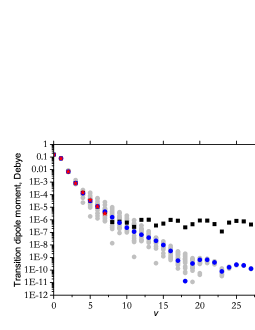
Figure 4: Vibrational transition dipole moments (D) from the $\varv=0$ ground state. of ¹⁴N¹⁶O: empirical (Lee et al., 2006) (stars) and ab initio calculated using the quintic splines (squares) and Padé-type expansion (circles).

where $z=r/r_{\rm e}$, $T_{i}(x)$ are Chebyshev polynomials and $a_{i}$ are expansion parameters obtained by fitting to 352 ab initio dipole moment values covering $r=0.7-9$ Å. With 18 parameters we were able to reproduce the ab initio dipole with a root-mean-square (rms) error of 0.07 D for the whole range, with best agreement in the vicinity of the equilibrium of the order $10^{-5}-10^{-6}$ D. The vibrational transition moments computed using the quintic splines interpolation implemented as default in Duo and this Padé expression are shown in Fig. 4, where they are also compared to the empirical values, see Lee et al. (2006) and references therein, where available. They are also listed in Table 8. The spline-interpolated dipoles produce an artificial plateau-like error of $10^{-6}$–$10^{-7}$ D as expected (Li et al., 2015). The analytical form improves this by shifting the error to $10^{-10}$–$10^{-11}$ D. However, the transition dipole moment values appear to be very sensitive to such functional interpolation, at least within $10^{-5}-10^{-6}$ D, which is also the absolute error of our interpolation scheme. To illustrate this, Fig. 4 also shows vibrational transition dipole moments, computed using fits with different expansion orders, ranges, weighings of the data, etc. From all these combinations we then selected the set which gives the closest agreement with the transition dipole moments obtained using the spline-interpolation scheme. This set is also in the best agreement with the empirical transition dipole moments.

In intensity (line list) calculations we used a dipole threshold of $1\times 10^{-9}$ D, i.e. all vibrational matrix elements smaller than this value were set to zero to avoid artificial intensities due to the numerical error.

Table 8: Transition dipole moments of NO. The total uncertainties are given in parenthesis. The ab initio  values are obtained using the ab initio DMC interpolated with the quintic splines and Padé expression as in Eq. (5).

Band			‘Exp’	Ref.	Splines	Padé
0– 0			0.1595(15)	Amiot (1982)	0.155	0.155
1– 0	$10^{-2}$	$\times$	7.6931(14)	Coudert et al. (1995)	7.649	7.646
2– 0	$10^{-3}$	$\times$	6.78(20)	Mandin et al. (1997)	6.865	6.890
3– 0	$10^{-4}$	$\times$	7.975(23)	Lee et al. (2006)	8.372	8.379
4– 0	$10^{-4}$	$\times$	1.4804(45)	Lee et al. (2006)	1.396	1.300
5– 0	$10^{-5}$	$\times$	3.683(17)	Lee et al. (2006)	3.319	3.244
6– 0	$10^{-5}$	$\times$	1.136(06)	Lee et al. (2006)	1.100	1.182
7– 0	$10^{-6}$	$\times$	3.09(47)	Bood et al. (2006)	3.959	4.458
3– 1	$10^{-2}$	$\times$	1.19(12)	Mandin et al. (1998)		1.194
2– 1			0.109(38)	Dana et al. (1994)		0.108
7– 6	$10^{-1}$	$\times$	1.89(11)	Drabbels & Wodtke (1997)		1.965
21– 20	$10^{-1}$	$\times$	3.176(82)	Drabbels & Wodtke (1997)		3.015
21– 19	$10^{-1}$	$\times$	1.077(27)	Drabbels & Wodtke (1997)		1.047
21– 18	$10^{-2}$	$\times$	3.68(16)	Drabbels & Wodtke (1997)		3.220
21– 17	$10^{-2}$	$\times$	1.09(16)	Drabbels & Wodtke (1997)		1.239

Our final Duo input, which defines our final PEC, SOC and DMC as well as other input parameters selected, is given in the supplementary data.

2.5.2 Hybrid Line List

The final lists were produced by combining the SPCAT frequencies and Duo Einstein coefficients. To this end we used the advantage of the two-file structure of the ExoMol format (Tennyson et al., 2016c), with .states and .trans files. We simply replaced the Duo energies in the states file with the corresponding SPCAT values. The corresponding coverage of SPCAT and Duo is summarized in Table 13. The correlation based on the Hund’s case (a) quantum numbers ($J,\varv,\Omega$ and parity) was straightforward. The Duo energies extend significantly beyond the SPCAT data range. In order to prevent possible jumps and discontinuities when switching between these data set, the Duo energies were shifted to match the SPCAT energies at the points of the switch. For example, in case of ¹⁴N¹⁶O, the maximum vibrational excitation considered by SPCAT $\varv_{\rm max}$ is 29 (the switching point), therefore all Duo energies for $v=29\ldots 51$ where shifted such that Duo $\varv=29$ energy value coincides with those by SPCAT for all $J$s. The same strategy was used to stitch the SPCAT and Duo energies at $J=99.5$ (the chosen threshold for SPCAT): the Duo values for $J=99.5\ldots 185.5$ were shifted to match the corresponding $J=99.5$ value of SPCAT for each $\varv$, $\Omega$ and parity individually.

The SPCAT energies of the isotopologues are even more limited in terms of the vibrational coverage; $\varv_{\rm max}$ = 9 (¹⁵N¹⁶O and ¹⁴N¹⁸O) and $\varv_{\rm max}$ = 4 (¹⁴N¹⁷O, ¹⁵N¹⁷O and ¹⁵N¹⁸O). As for the main isotopologue, we used the corresponding Duo energies to top up the corresponding line list to the same thresholds as for ¹⁴N¹⁶O. The better representation of the data from the parent isotopologue helped us to improve the accuracy of the Duo prediction for $v\leq 29$. By comparing the SPCAT and Duo energies of ¹⁴N¹⁶O in this range, the corresponding residuals were propagated (for each rovibronic state individually) to correct the corresponding Duo energies for the other five isotopologues (see, for example, Polyansky et al. (2016)). The energies for $\varv\geq\varv_{\rm max}$ were then given by:

$$E_{J,\pm,v,\Omega}^{\rm iso}=E_{J,\pm,v,\Omega}^{\rm Duo-iso}+E_{J,\pm,v,\Omega}^{\rm SPCAT-parent}-E_{J,\pm,v,\Omega}^{\rm Duo-parent},$$

where ‘Duo-iso’ refers to the Duo energies of one of the five isotopologues for a given set of $J,\pm,v,\Omega$, while ‘Duo-parent’ and ‘SPCAT-parent’ indicate the corresponding energies of the parent isotopologue computed by Duo and SPCAT, respectively. The line lists do not include the hyperfine structure of the energy levels and transitions.

Table 9: Extract from the states file of the ¹⁴N¹⁶O line list.

$i$	Energy (cm-1)	$g_{i}$	$J$	$\tau$	$g_{J}$	Parity	e/f	State	$\varv$	${\Lambda}$	${\Sigma}$	${\Omega}$	emp/calc
1	0.000000	6	0.5	inf	-0.000767	+	e	X1/2	0	1	-0.5	0.5	e
2	1876.076228	6	0.5	8.31E-02	-0.000767	+	e	X1/2	1	1	-0.5	0.5	e
3	3724.066346	6	0.5	4.25E-02	-0.000767	+	e	X1/2	2	1	-0.5	0.5	e
4	5544.020643	6	0.5	2.89E-02	-0.000767	+	e	X1/2	3	1	-0.5	0.5	e
5	7335.982597	6	0.5	2.22E-02	-0.000767	+	e	X1/2	4	1	-0.5	0.5	e
6	9099.987046	6	0.5	1.81E-02	-0.000767	+	e	X1/2	5	1	-0.5	0.5	e
7	10836.058173	6	0.5	1.54E-02	-0.000767	+	e	X1/2	6	1	-0.5	0.5	e
8	12544.207270	6	0.5	1.35E-02	-0.000767	+	e	X1/2	7	1	-0.5	0.5	e
9	14224.430238	6	0.5	1.21E-02	-0.000767	+	e	X1/2	8	1	-0.5	0.5	e
10	15876.704811	6	0.5	1.10E-02	-0.000767	+	e	X1/2	9	1	-0.5	0.5	e
11	17500.987446	6	0.5	1.01E-02	-0.000767	+	e	X1/2	10	1	-0.5	0.5	e
12	19097.209871	6	0.5	9.41E-03	-0.000767	+	e	X1/2	11	1	-0.5	0.5	e
13	20665.275246	6	0.5	8.83E-03	-0.000767	+	e	X1/2	12	1	-0.5	0.5	e
14	22205.053904	6	0.5	8.35E-03	-0.000767	+	e	X1/2	13	1	-0.5	0.5	e
15	23716.378643	6	0.5	7.94E-03	-0.000767	+	e	X1/2	14	1	-0.5	0.5	e
16	25199.039545	6	0.5	7.59E-03	-0.000767	+	e	X1/2	15	1	-0.5	0.5	e
17	26652.778266	6	0.5	7.30E-03	-0.000767	+	e	X1/2	16	1	-0.5	0.5	e
18	28077.281796	6	0.5	7.05E-03	-0.000767	+	e	X1/2	17	1	-0.5	0.5	e
19	29472.175632	6	0.5	6.84E-03	-0.000767	+	e	X1/2	18	1	-0.5	0.5	e
20	30837.016339	6	0.5	6.66E-03	-0.000767	+	e	X1/2	19	1	-0.5	0.5	e
21	32171.283479	6	0.5	6.50E-03	-0.000767	+	e	X1/2	20	1	-0.5	0.5	e
22	33474.370850	6	0.5	6.38E-03	-0.000767	+	e	X1/2	21	1	-0.5	0.5	e
23	34745.577033	6	0.5	6.27E-03	-0.000767	+	e	X1/2	22	1	-0.5	0.5	e
24	35984.095189	6	0.5	6.19E-03	-0.000767	+	e	X1/2	23	1	-0.5	0.5	e
25	37189.002091	6	0.5	6.13E-03	-0.000767	+	e	X1/2	24	1	-0.5	0.5	e
26	38359.246347	6	0.5	6.09E-03	-0.000767	+	e	X1/2	25	1	-0.5	0.5	e
27	39493.635791	6	0.5	6.07E-03	-0.000767	+	e	X1/2	26	1	-0.5	0.5	e

$i$: State counting number.

$\tilde{E}$: State energy in cm^-1.

$g$: Total statistical weight, equal to ${g_{\rm ns}(2J+1)}$.

$J$: Total angular momentum.

$\tau$: Lifetime (s^-1).

$g_{J}$: Landé $g$-factor

$+/-$: Total parity.

$e/f$: Rotationless parity.

State: Electronic state.

$\varv$: State vibrational quantum number.

$\Lambda$: Projection of the electronic angular momentum.

$\Sigma$: Projection of the electronic spin.

$\Omega$: $\Omega=\Lambda+\Sigma$, projection of the total angular momentum.

emp/calc: e= empirical (SPCAT), c=calculated (Duo).

Table 10: Extract from the transitions file of the ¹⁴N¹⁶O line list.

$f$	$i$	$A_{fi}$ (s-1)	$\tilde{\nu}_{fi}$
14123	13911	1.5571E-02	10159.167959
13337	13249	5.9470E-06	10159.170833
1483	1366	3.7119E-03	10159.177466
9072	8970	1.1716E-04	10159.177993
1380	1469	3.7119E-03	10159.178293
14057	13977	1.5571E-02	10159.179386
10432	10498	4.5779E-07	10159.187818
12465	12523	5.4828E-03	10159.216008
20269	20286	1.2448E-10	10159.227463
12393	12595	5.4828E-03	10159.231009
2033	2111	6.4408E-04	10159.266541
17073	17216	4.0630E-03	10159.283484
5808	6085	3.0844E-02	10159.298459
5905	5988	3.0844E-02	10159.302195
13926	13845	1.5597E-02	10159.312986

$f$: Upper state counting number;
$i$: Lower state counting number;
$A_{fi}$: Einstein-A coefficient in s^-1;
$\tilde{\nu}_{fi}$: transition wavenumber in cm^-1.

3 Results

3.1 Partition Function

The partition function is given by

$$Q(T)=g_{\rm ns}\sum\limits^{n}_{i=0}(2J_{i}+1)\exp\Big{(}\frac{-c_{2}\tilde{E}_{i}}{T}\Big{)},$$ (6)

$\tilde{E_{i}}$ is the energy term value (cm^-1); $c_{2}$ is the second radiation constant (K cm); and $g_{\rm ns}$ is the nuclear statistical weight. This was calculated from the new line list using the in-house program ExoCross (Yurchenko, 2017) up to a temperature of 5000 K in increments of 1 K. Tabulations of this form are given in the supplementary material for all six of the isotopologues considered.

The computed partition function compares well to the values by Sauval & Tatum (1984), above their lower temperature limit of 1000 K, as shown in Fig. 5. Slight disagreement at higher temperatures may be due to the fact that only the ground electronic state of NO has been considered in the Duo calculations, since excited states will have a larger contribution at high temperatures. Looking at the log-plot comparison, disagreement below $\log(T)$ = 3.0 corresponds to temperatures lower than 1000 K, for which the Sauval and Tatum model is not valid (see also Table 11, where the partition functions for temperatures are compared).

Table 11: Partition functions of NO: HITRAN values (TIPS) (Gamache et al., 2000) (provided only between 70 and 3000 K), obtained using parameters from Sauval & Tatum (1984) and Duo values.

$T$ (K)	HITRAN	Sauval & Tatum	Duo
70	189.75	492.80	193.53
100	293.36	585.91	296.51
300	1160.75	1296.85	1159.66
1000	4877.73	4874.19	4877.53
1500	8403.66	8470.16	8424.34
2000	12812.56	12951.71	12887.04
2500	18135.16	18343.44	18311.46
3000	24382.24	24673.57	24726.00
4000		40270.57	40622.12
5000		59994.10	60769.42

The partition function was also represented using the following functional form (Vidler & Tennyson, 2000) given by

$$\log_{10}Q(T)=\sum\limits^{10}_{n=0}a_{n}(\log_{10}T)^{n}.$$ (7)

This expression was used to least-squares fit eleven expansion coefficients, $a_{0},\ldots,a_{10}$, to the Duo partition function. An example of expansion parameters for ¹⁴N¹⁶O are presented in Table 12. These parameters reproduce the temperature dependence of partition function of NO within within 0.3% for most of the data, however it increases to just 0.4% at $T$ = 4000 K and 1.1% at $T$ = 5000 K. This is still a very small error, and thus the fit can be said to reliably reproduce the partition function. Expansion parameters for all six species are included into the supplementary materials.

Table 12: Expansion coefficients for the partition function of ¹⁴N¹⁶O given by Eq. (7). Parameters for other isotopologues can be found in the supplementary material.

Expansion coefficient
$a_{0}$	1.0761409513
$a_{1}$	-0.1681972157
$a_{2}$	1.5810964843
$a_{3}$	-4.5662697659
$a_{4}$	9.4920289544
$a_{5}$	-10.9491757465
$a_{6}$	7.3756190305
$a_{7}$	-2.9829630362
$a_{8}$	0.7131937052
$a_{9}$	-0.0928960661
$a_{10}$	0.0050821171

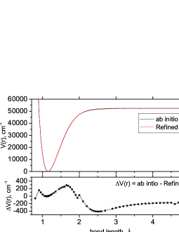
Figure 5: Comparison of the calculated partition function (solid line) and that modelled by Sauval & Tatum (1984) (dashed line) up to 5000 K.

3.2 Intensities

The absorption line intensities were obtained using (Bernath, 2005)

$$I=\frac{1}{8\pi c\tilde{\nu}^{2}}\frac{g_{\rm ns}(2J^{\prime}+1)}{Q(T)}\hskip 4.2679ptA_{if}\hskip 4.2679pt\exp\Bigg{(}{\frac{-c_{2}\tilde{E}^{\prime\prime}}{T}}\Bigg{)}\Bigg{[}1-\exp\Bigg{(}{\frac{c_{2}\tilde{\nu}}{T}}\Bigg{)}\Bigg{]},$$ (8)

where $I$ is the line intensity (cm molecule^-1); $c$ is the speed of light (cm $s^{-1}$); $Q(T)$ is the partition function; $\tilde{E}^{\prime\prime}$ is the lower state term value; $c_{2}$ is the second radiation constant (K cm); and $g_{\rm ns}$ is the nuclear statistical weight.

Absorption intensities were calculated using ExoCross and the lines are presented as stick spectra. Figure 6 compares the computed absorption intensities to intensities from HITRAN at 296 K (Rothman et al., 2013) up to a wavenumber of 15,000 cm^-1. It can be seen that the absorption intensities calculated in this work are in excellent agreement with those of the HITRAN database, as they are of the same strength and wavenumber; this work is more comprehensive, as absorption intensities are calculated up to 40,000 cm^-1 whilst the HITRAN database employs a cut-off wavenumber of approximately 10,000 cm^-1. It should be noted that the HITRAN data is reasonably complete at $T=$ 296 K for ¹⁴N¹⁶O, but not for other isotopologues (see Table 13). HITRAN also contains a huge number of extremely weak (at 296 K) transitions (down to $10^{-95}$ cm/molecule). Many of the strong lines are with the hyperfine structure resolved. After excluding the weak lines (using the HITRAN cut-off algorithm (Rothman et al., 2013)) and averaging over the hyperfine components, we have obtained about 6,400 transitions ($T=296$ K). This can be compared to 8,274 lines in our ¹⁴N¹⁶O line list at 296 K (using the same HITRAN cut-off). This and other comparisons are summarised in Table 13.

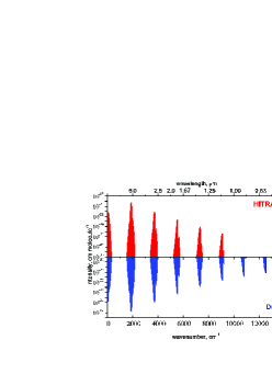
Figure 6: Log-scale comparison of absorption intensities ($\mathrm{cm\hskip 2.84526ptmolecule^{-1}}$) at $T$ = 296 K of the HITRAN database (Rothman et al., 2013) (red) and this work (blue). Each intensity ‘column’ represents a vibrational band.

Comparison of band structure is presented in Fig. 7, again comparing this work to the HITRAN database. The pure rotational band is present in the far-infrared region, the fundamental band is is the mid-infrared region and the first and second vibrational overtones are present in the near-infrared region. Branch structure is visible, with the extent of the $P$-branch increasing with each successive overtone, whilst the $R$-branch becomes more dense, as expected (Hollas, 2004). The fundamental band is the strongest, while the band intensity decreases with each successive overtone as expected.

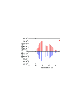
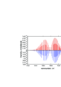
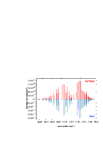
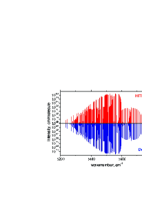
Figure 7: Stick spectra comparison of HITRAN absorption intensities (cm/molecule) (red) and absorption intensities calculated in this work (blue), at a temperature of 296 K: pure rotational band, fundamental vibrational band, 1st vibrational overtone band and 2nd vibrational overtone band. Intensity strength and wavenumber positions are in excellent agreement.

3.2.1 Isotopologue Intensity Comparison

For comparison purposes, intensities were calculated using the same procedure for the ¹⁵N¹⁸O isotopologue; the fundamental vibrational band is compared to the same region of the NO spectrum in Fig.  8. Since the reduced mass $\mu$ is less for the ¹⁵N¹⁸O isotopologue, it follows that the vibrational frequency and band origin is decreased. As a consequence, the absorption intensities are slightly weaker, since the Einstein A coefficients are proportional to the wavenumber cubed. This can be seen in Fig. 8, as the ¹⁵N¹⁸O band is shifted to a lower wavenumber, and intensities are slightly weakened.

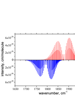
Figure 8: Stick spectrum comparison of the ¹⁵N¹⁸O fundamental vibrational band (red) and the ¹⁴N¹⁶O fundamental vibrational band (blue) in the 5.3 $\mu$m region at 296 K. Note that the ¹⁵N¹⁸O band is shifted to lower wavenumbers, and intensities are slightly weakened.

Table 13: A summary of the ExoMol isotopologue line lists (number of lines and states) and summary of on the SPCAT data (number of states and $\varv_{\rm max}$). $J_{\rm max}$ = 185.5 (ExoMol) and $J_{\rm max}$ = 99.5 (SPCAT). $\varv_{\rm max}$(ExoMol) = 51. ‘Abund’ refers to terrestrial isotopic abundances. $N_{296}$ gives the number of NO transitions in our line lists at 296 K after after applying the HITRAN intensity cutoff. $N_{\rm Trans.}$ are the corresponding numbers of lines in HITRAN 2012 (Rothman et al., 2013) (neglecting hyperfine structure).

		ExoMol			SPCAT		HITRAN
isotopologue	Abund	$N_{\rm States}$	$N_{\rm Trans.}$	$N_{296}$	$N_{\rm States}$	$\varv_{\rm max}$	$N_{296}$	$N_{\rm Trans.}$
14N16O	0.995	21,688	2,281,042	8,274	11,940	29	93,622	6,369
14N17O	0.000379	22,292	2,378,578	3,067	1,990	4
14N18O	0.00205	22,848	2,471,705	3,853	3,980	9	679	679
15N16O	0.00363	22,466	2,408,920	4,233	3,980	9	699	699
15N17O	0.00000138	23,106	2,516,634	1,290	1,990	4
15N18O	0.00000746	23,698	2,619,513	1,790	1,990	4

3.3 Cross-Sections

Figure 9 shows absorption cross-sections computed at temperatures of 300 K, 500 K, 1000 K, 2000 K and 3000 K using ExoCross for the wavelength range up to 0.2 $\mu$m. A Gaussian line profile was specified, with a half width at half maximum (HWHM) of 1 cm^-1. The intensities drop with the wavenumber (overtones) exponentially as they should (Li et al., 2015) up to 40000 cm^-1 (the upper bound in our line lists), after which plateau-like structures start forming at very small intensities ($<10^{-40}$ cm$/$molecule). The latter indicates the artifacts in our dipole at very high vibrational excitations. Transitions with wavelength less than 0.25 $\mu$m, indicated by the shaded area in 9, are are not included in the NO line lists.

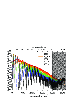
Figure 9: Absorption spectrum of the ground state of ¹⁴N¹⁶O as a function of temperature. The temperatures considered are 300 K (bottom), 500 K, 1000 K, 2000 K and 3000 K (top). Cross-sections are calculated with a Gaussian profile and HWHM = 1 cm^-1. The higher-temperature profiles will be useful in characterising the spectra of terrestrial exoplanets and brown dwarfs.

Absorption cross-sections of ¹⁴N¹⁶O with a Doppler profile were computed from the HITEMP database for $T$ = 3000 K, in the range 0 – 14,000 cm^-1 and compared to cross-sections generated using the ¹⁴N¹⁶O ExoMol line list, see Fig. 10. There is a good general agreement in strength and wavenumber between the two spectra. Again, it should be noted that this work is more extensive, as the HITEMP database employs a cut-off wavenumber of approximately 10,000 cm^-1, as does the HITRAN database.

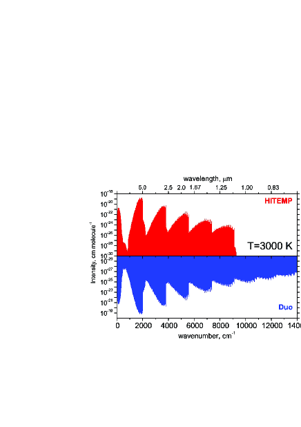
Figure 10: Comparison of absorption cross-sections (cm²/molecule) with a Doppler line profile at 3000 K of the HITEMP database (Rothman et al., 2010) (red) and this work (blue).

3.4 Radiative Lifetimes

The radiative lifetime of an excited state, $\tau_{i}$, can be computed in a straightforward manner from the state and transition files (Tennyson et al., 2016a) by

$$\tau_{i}=\frac{1}{\sum\limits_{f<i}A_{if}}$$ (9)

where $A_{if}$ is the Einstein A coefficient, and $i$ and $f$ indicate the initial and final states, respectively. Lifetimes were calculated by the program ExoCross. The computed lifetimes are plotted in Fig. 11 as a function of wavenumber (cm^-1); lifetimes for all states are plotted in grey, whilst lifetimes for the $\varv=0-3$ states are highlighted by coloured triangles. Lifetimes for states for which all downwards transitions are considered are given as part of the enhanced ExoMol states file (Tennyson et al., 2016c) as illustrated in Table 9 .

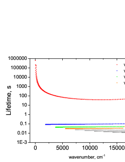
Figure 11: A log-plot of ¹⁴N¹⁶O radiative lifetimes against state energy. Lifetimes for states with $\varv=0-3$ are indicated by triangles while lifetimes for higher vibrational states are indicated by circles.

4 Discussion and Conclusion

The line list called NOname for the ground state of the NO isotopologue ¹⁴N¹⁶O was constructed using a hybrid (variational/effective Hamiltonian) scheme. The line list contains 21,688 states and 2,409,810 transitions in the wavenumber range 0–40,000 cm^-1, extending to maximum quantum numbers ${J=184.5}$ and ${v=51}$. Line lists were also constructed for the five isotopologues, ¹⁴N¹⁷O, ¹⁴N¹⁸O, ¹⁵N¹⁶O, ¹⁵N¹⁷O and ¹⁵N¹⁸O in the same range and containing similar numbers of states and transitions.

Initial energy levels in the line lists were calculated by a fit of ab initio results using experimental energies. Refinement of the energy levels returned an rms of 0.015 cm^-1, which corresponds to a fit which is accurate to 0.02 cm^-1 for 80% of the data, whilst the worst residual is 0.13 cm^-1. These were then replaced by semi-empirical energies, where available. The accuracy of the energy levels propagates through to the computed line lists; comparison of intensities from this work and the HITRAN (Rothman et al., 2013) database for the ¹⁴N¹⁶O isotopologue at 296 K show excellent agreement both in strength and position of lines. Because most of the Duo energies were replaced with the semi-empirical ones, the fit was mostly done to improve the accuracy of intensities via better quality of the corresponding wavefunctions. Only highly excited states ($J>100.5$ and $\varv>29$ for ¹⁴N¹⁶O) were taken from the Duo calculations, shifted at the stitching points to avoid discontinuities. Thus our ¹⁴N¹⁶O line positions can be considered of experimental accuracy for $\varv\leq 22$, which is then expected to degrade gradually when extrapolated to $\varv=22\ldots 51$. The difference between SPCAT and Duo at $\varv=29$ (the stitching point) is 2.47 cm^-1, after which we rely on the Duo extrapolation. It should be noted, however, that the impact from the energies in the extrapolated region is marginal for practical applications due the low absorption intensities of the corresponding transitions. For the example, the overtones with $\varv^{\prime}>29$ fall into the wavenumber region above 40,000 cm^-1, which is fully excluded from -the line list. We keep the corresponding energies anyway for the sake of completeness.

The partition function $Q(T)$ was calculated for the ¹⁴N¹⁶O isotopologue, and compared to that computed by Sauval & Tatum (1984); there is good agreement above 1000 K, below which the Sauval and Tatum model is not valid. Slight disagreement at high temperatures is likely due to the fact that only the ground state of NO is considered in this work, since excited states will have a larger contribution to the partition function at high temperatures. An idea for future work is to compute line lists for the excited states, and to model the interaction between these states, in order to improve the accuracy of the line list at high rotational and vibrational energy levels.

Lifetimes were calculated for all energy levels considered. Absorption cross-sections have been calculated for temperatures ranging from 300 K $-$ 5000 K. The absorption spectrum at 3000 K is in excellent agreement with but much more extensive than the same spectrum calculated from the HITEMP database (Rothman et al., 2010), illustrating that the line list is also accurate at high temperatures. The absorption spectra will be applied in the characterisation of high-temperature astronomical objects such as exoplanet atmospheres, brown dwarfs and cool stars. The NO spectra may also be useful in the remote sensing of high temperature events in the Earth’s atmosphere such as lightning and vehicle re-entry from orbit. Our calculations also provide Landé $g$-factors for each state; a comparison of these values with observed (Ionin et al., 2011) Zeeman splitting of NO states in weak magnetic fields was carried out by Semenov et al. (2017), and found very good agreement.

The six NO line lists are the most comprehensive available; they extend up to a wavenumber of 40,000 cm^-1, compared to the upper limit of 10,000 cm^-1 in both the HITRAN and HITEMP databases (Rothman et al., 2010; Rothman et al., 2013). These line lists can be downloaded from the CDS, via ftp://cdsarc.u-strasbg.fr/pub/cats/J/MNRAS/, or http://cdsarc.u-strasbg.fr/viz-bin/qcat?J/MNRAS/, or from www.exomol.com. On the ExoMol website we also provide a script to convert the line list into the native HITRAN format.

References

- Ackermann & Miescher (1969) Ackermann F., Miescher E., 1969, J. Mol. Spectrosc., 31, 400
- Amano (2010) Amano T., 2010, ApJ, 716, L1
- Amiot (1982) Amiot C., 1982, J. Mol. Spectrosc., 94, 150
- Amiot & Guelachvili (1979) Amiot C., Guelachvili G., 1979, J. Mol. Spectrosc., 76, 86
- Amiot & Verges (1980) Amiot C., Verges J., 1980, J. Mol. Spectrosc., 81, 424
- Amiot et al. (1978) Amiot C., Bacis R., Guelachvili G., 1978, Can. J. Phys., 56, 251
- Ardaseva et al. (2017) Ardaseva A., Rimmer P. B., Waldmann I., Rocchetto M., Yurchenko S. N., Helling C., Tennyson J., 2017, MNRAS
- Asvany et al. (2008) Asvany O., Ricken O., Müller H. S. P., Wiedner M. C., Giesen T. F., Schlemmer S., 2008, Phys. Rev. Lett., 100, 233004
- Balabanov & Peterson (2005) Balabanov N. B., Peterson K. A., 2005, J. Chem. Phys., 123, 064107
- Balabanov & Peterson (2006) Balabanov N. B., Peterson K. A., 2006, J. Chem. Phys., 125, 074110
- Barman et al. (2015) Barman T. S., Konopacky Q. M., Macintosh B., Marois C., 2015, ApJ, 804, 61
- Barry & Chorley (2010) Barry R. G., Chorley R. J., 2010, Atmosphere, Weather and Climate, 9 edn. Van Nostrand Reinhold Company, London and New York
- Barton et al. (2013) Barton E. J., Yurchenko S. N., Tennyson J., 2013, MNRAS, 434, 1469
- Barton et al. (2014) Barton E. J., Chiu C., Golpayegani S., Yurchenko S. N., Tennyson J., Frohman D. J., Bernath P. F., 2014, MNRAS, 442, 1821
- Beaulieu et al. (2011) Beaulieu J. P., et al., 2011, ApJ, 731, 16
- Bernath (2005) Bernath P. F., 2005, Spectra of Atoms and Molecules, 2nd edn. Oxford University Press
- Bood et al. (2006) Bood J., McIlroy A., Osborn D. L., 2006, J. Chem. Phys., 124
- Brooke et al. (2015) Brooke J. S. A., Bernath P. F., Western C. M., 2015, J. Chem. Phys., 143, 026101
- Brooke et al. (2016) Brooke J. S. A., Bernath P. F., Western C. M., Sneden C., Afşar M., Li G., Gordon I. E., 2016, J. Quant. Spectrosc. Radiative Transfer, 168, 142
- Brooke et al. (2014) Brooke J. S. A., Ram R. S., Western C. M., Li G., Schwenke D. W., Bernath P. F., 2014, ApJS, 210, 23
- Brown & Merer (1979) Brown J. M., Merer A. J., 1979, J. Mol. Spectrosc., 74, 488
- Brown et al. (1979) Brown J. M., Colbourn E. A., Watson J. K. G., Wayne F. D., 1979, J. Mol. Spectrosc., 74, 294
- Burrows et al. (2002) Burrows A., Ram R. S., Bernath P., Sharp C. M., Milsom J. A., 2002, ApJ, 577, 986
- Burrows et al. (2005) Burrows A., Dulick M., Bauschlicher C. W., Bernath P. F., Ram R. S., Sharp C. M., Milsom J. A., 2005, ApJ, 624, 988
- Callear & Pilling (1970) Callear A. B., Pilling M. J., 1970, Trans. Faraday Soc., 66, 1618
- Campargue et al. (2015) Campargue A., Karlovets E. V., Kassi S., 2015, J. Quant. Spectrosc. Radiat. Transf., 154, 113
- Canty et al. (2015) Canty J. I., et al., 2015, MNRAS, 450, 454
- Coudert et al. (1995) Coudert L. H., Dana V., Mandin J. Y., Morillonchapey M., Farrenq R., 1995, J. Mol. Spectrosc., 172, 435
- Cox et al. (2008) Cox C., Saglam A., Gerard J. C., Bertaux J. L., Gonzalez-Galindo F., Leblanc F., Reberac A., 2008, J. Geophys. Res.: Planets, 113, E08012
- Cushing et al. (2011) Cushing M. C., et al., 2011, ApJ, 743, 50
- Dale et al. (1977) Dale R. M., Johns J. W. C., McKellar A. R. W., Riggin M., 1977, J. Mol. Spectrosc., 67, 440
- Dana et al. (1994) Dana V., Mandin J. Y., Coudert L. H., Badaoui M., Leroy F., Guelachvili G., Rothman L. S., 1994, J. Mol. Spectrosc., 165, 525
- Danielak et al. (1997) Danielak J., Domin U., Kepa R., Rytel M., Zachwieja M., 1997, J. Mol. Spectrosc., 181, 394
- Devivie & Peyerimhoff (1988) Devivie R., Peyerimhoff S. D., 1988, J. Chem. Phys., 89, 3028
- Drabbels & Wodtke (1997) Drabbels M., Wodtke A. M., 1997, J. Chem. Phys., 106, 3024
- Drouin et al. (2001) Drouin B. J., Miller C. E., Müller H. S. P., Cohen E. A., 2001, J. Mol. Spectrosc., 205, 128
- Dulick et al. (2003) Dulick M., Bauschlicher C. W., Burrows A., Sharp C. M., Ram R. S., Bernath P., 2003, ApJ, 594, 651
- Eastes et al. (1992) Eastes R. W., Huffman R. E., Leblanc F. J., 1992, Planet Space Sci., 40, 481
- Farhat (2017) Farhat A., 2017, MNRAS
- Flagan & Seinfeld (1988) Flagan R. C., Seinfeld J. H., 1988, Fundamentals of Air Pollution Engineering, 1 edn. Prentice Hall, New Jersey
- Furtenbacher & Császár (2012a) Furtenbacher T., Császár A. G., 2012a, J. Quant. Spectrosc. Radiat. Transf., 113, 929
- Furtenbacher & Császár (2012b) Furtenbacher T., Császár A. G., 2012b, J. Molec. Struct. (THEOCHEM), 1009, 123
- Furtenbacher et al. (2007) Furtenbacher T., Császár A. G., Tennyson J., 2007, J. Mol. Spectrosc., 245, 115
- Furtenbacher et al. (2016) Furtenbacher T., Szabó I., Császár A. G., Bernath P. F., Yurchenko S. N., Tennyson J., 2016, ApJS, 224, 44
- Gamache et al. (2000) Gamache R. R., Kennedy S., Hawkins R., Rothman L. S., 2000, J. Mol. Spectrosc., 517, 407
- GharibNezhad et al. (2013) GharibNezhad E., Shayesteh A., Bernath P. F., 2013, MNRAS, 432, 2043
- Goodisman (1963) Goodisman J., 1963, J. Chem. Phys., 38, 2597
- Halfen & Ziurys (2015) Halfen D. T., Ziurys L. M., 2015, ApJ, 814, 119
- Hallin et al. (1979) Hallin K.-E. J., Johns J. W. C., Lepard D. W., Mantz A. W., Wall D. L., Narahari Rao K., 1979, J. Mol. Spectrosc., 74, 26
- Henry et al. (1978) Henry A., Le Moal M. F., Cardinet P., Valentin A., 1978, J. Mol. Spectrosc., 70, 18
- Hinz et al. (1986) Hinz A., Wells J. S., Maki A. G., 1986, J. Mol. Spectrosc., 119, 120
- Hollas (2004) Hollas J. M., 2004, Modern Spectroscopy, 4 edn. Wiley, Chichester
- Ionin et al. (2011) Ionin A. A., Klimachev Y. M., Kozlov A. Y., Kotkov A. A., 2011, J. Phys. B: At. Mol. Opt. Phys., 44, 025403
- James (1964) James T. C., 1964, J. Chem. Phys., 40, 762
- James & Thibault (1964) James T. C., Thibault R. J., 1964, J. Chem. Phys., 41, 2806
- Klaus et al. (1996) Klaus T., Saleck A. H., Belov S. P., Winnewisser G., Hirahara Y., Hayashi M., Kagi E., Kawaguchi K., 1996, J. Mol. Spectrosc., 180, 197
- Le Roy & Huang (2002) Le Roy R. J., Huang Y. Y., 2002, J. Molec. Struct. (THEOCHEM), 591, 175
- Le Roy et al. (2011) Le Roy R. J., Haugen C. C., Tao J., Li H., 2011, Mol. Phys., 109, 435
- Lee et al. (1999) Lee E. G., Seto J. Y., Hirao T., Bernath P. F., Le Roy R. J., 1999, J. Mol. Spectrosc., 194, 197
- Lee et al. (2006) Lee Y. P., Cheah S. L., Ogilvie J. F., 2006, Infrared Physics & Technology, 47, 227
- Li et al. (2012) Li G., Harrison J. J., Ram R. S., Western C. M., Bernath P. F., 2012, J. Quant. Spectrosc. Radiat. Transf., 113, 67
- Li et al. (2015) Li G., Gordon I. E., Rothman L. S., Tan Y., Hu S.-M., Kassi S., Campargue A., Medvedev E. S., 2015, ApJS, 216, 15
- Liu et al. (2001) Liu Y., Guo Y., Lin J., Huang G., Duan C., Li F., 2001, Mol. Phys., 99, 1457
- Lodi & Tennyson (2010) Lodi L., Tennyson J., 2010, J. Phys. B: At. Mol. Opt. Phys., 43, 133001
- Lodi et al. (2008) Lodi L. L., Polyansky O. L., Tennyson J., 2008, Mol. Phys., 106, 1267
- Lodi et al. (2015) Lodi L., Yurchenko S. N., Tennyson J., 2015, Mol. Phys., 113, 1998
- Lovas & Tiemann (1974) Lovas F. J., Tiemann E., 1974, J. Phys. Chem. Ref. Data, 3, 609
- Lowe et al. (1981) Lowe R. S., McKellar A. R. W., Veillette P., Meerts W. L., 1981, J. Mol. Spectrosc., 88, 372
- Mandin et al. (1994) Mandin J. Y., Dana V., Coudert L. H., Badaoui M., Leroy F., Morillonchapey M., Farrenq R., Guelachvili G., 1994, J. Mol. Spectrosc., 167, 262
- Mandin et al. (1997) Mandin J. Y., Dana V., Regalia L., Barbe A., Thomas X., 1997, J. Mol. Spectrosc., 185, 347
- Mandin et al. (1998) Mandin J. Y., Dana V., Regalia L., Barbe A., Von der Heyden P., 1998, J. Mol. Spectrosc., 187, 200
- Martin et al. (2003) Martin S., Mauersberger R., Martin-Pintado J., Garcia-Burillo S., Henkel C., 2003, A&A, 411, L465
- Martin et al. (2006) Martin S., Mauersberger R., Martin-Pintado J., Henkel C., Garcia-Burillo S., 2006, ApJS, 164, 450
- McGonagle et al. (1990) McGonagle D., Ziurys L. M., Irvine W. M., Minh Y. C., 1990, ApJ, 359, 121
- McKemmish et al. (2016) McKemmish L. K., Yurchenko S. N., Tennyson J., 2016, MNRAS, 463, 771
- McKemmish et al. (2017) McKemmish L. K., et al., 2017, ApJS, 228, 15
- Medvedev et al. (2016) Medvedev E. S., Meshkov V. V., Stolyarov A. V., Ushakov V. G., Gordon I. E., 2016, J. Mol. Spectrosc., pp –
- Meerts (1976) Meerts W. L., 1976, Chem. Phys., 14, 421
- Meerts & Dymanus (1972) Meerts W. L., Dymanus A., 1972, J. Mol. Spectrosc., 44, 320
- Mohr et al. (2012) Mohr P. J., Taylor B. N., Newell D. B., 2012, Rev. Mod. Phys., 84, 1527
- Molliere et al. (2015) Molliere P., van Boekel R., Dullemond C., Henning T., Mordasini C., 2015, ApJ, 813, 47
- Mondelain et al. (2015) Mondelain D., Sala T., Kassi S., Romanini D., Marangoni M., Campargue A., 2015, J. Quant. Spectrosc. Radiat. Transf., 154, 35
- Morley et al. (2014) Morley C. V., Marley M. S., Fortney J. J., Lupu R., Saumon D., Greene T., Lodders K., 2014, ApJ, 787, 78
- Morley et al. (2015) Morley C. V., Fortney J. J., Marley M. S., Zahnle K., Line M., Kempton E., Lewis N., Cahoy K., 2015, ApJ, 815, 110
- Mount et al. (2010) Mount B. J., Müller H. S. P., Redshaw M., Myers E. G., 2010, Phys. Rev. A, 81, 064501
- Müller et al. (2005) Müller H. S. P., Schlöder F., Stutzki J., Winnewisser G., 2005, J. Molec. Struct. (THEOCHEM), 742, 215
- Müller et al. (2013) Müller H. S. P., Spezzano S., Bizzocchi L., Gottlieb C. A., Degli Esposti C., McCarthy M. C., 2013, J. Phys. Chem. A, 117
- Müller et al. (2014) Müller H. S. P., et al., 2014, A&A, 569, L5
- Müller et al. (2015) Müller H. S. P., Kobayashi K., Takahashi K., Tomaru K., Matsushima F., 2015, J. Mol. Spectrosc., 310, 92
- Neumann (1970) Neumann R. M., 1970, ApJ, 161, 779
- Patrascu et al. (2015) Patrascu A. T., Tennyson J., Yurchenko S. N., 2015, MNRAS, 449, 3613
- Paulose et al. (2015) Paulose G., Barton E. J., Yurchenko S. N., Tennyson J., 2015, MNRAS, 454, 1931
- Perryman (2014) Perryman M., 2014, The Exoplanet Handbook, 1 edn. Cambridge University Press, Cambridge
- Peterson & Dunning (2002) Peterson K. A., Dunning T. H., 2002, J. Chem. Phys., 117, 10548
- Pickett (1991) Pickett H. M., 1991, J. Mol. Spectrosc., 148, 371
- Pickett et al. (1979) Pickett H. M., Cohen E. A., Waters J. W., Phillips T. G., 1979, in Contribution 13, 34th International Symposium on Molecular Spectroscopy, Columbus, OH, USA. http://hdl.handle.net/1811/10845
- Polak & Fiser (2004) Polak R., Fiser J. F., 2004, Chem. Phys., 303, 73
- Polyansky et al. (2016) Polyansky O. L., Kyuberis A. A., Lodi L., Tennyson J., Ovsyannikov R. I., Zobov N., 2016, MNRAS, 466, 1363
- Rawlins et al. (1992) Rawlins W. T., Fraser M. E., Miller S. M., Blumberg W. A. M., 1992, J. Chem. Phys., 96, 7555
- Redshaw et al. (2009) Redshaw M., Mount B. J., Myers E. G., 2009, Phys. Rev. A, 79, 012507
- Rivlin et al. (2015) Rivlin T., Lodi L., Yurchenko S. N., Tennyson J., Le Roy R. J., 2015, MNRAS, 451, 634
- Rothman et al. (2010) Rothman L. S., et al., 2010, J. Quant. Spectrosc. Radiat. Transf., 111, 2139
- Rothman et al. (2013) Rothman L. S., et al., 2013, J. Quant. Spectrosc. Radiat. Transf., 130, 4
- Roy & Henderson (2007) Roy R. J. L., Henderson R. D. E., 2007, Mol. Phys., 105, 663
- Roy et al. (2009) Roy R. J. L., Dattani N. S., Coxon J. A., Ross A. J., Crozet P., Linton C., 2009, J. Chem. Phys., 131, 204309
- Royer et al. (2010) Royer E., Montmessin F., Bertaux J.-L., 2010, Planet Space Sci., 58, 1314
- Saleck et al. (1991) Saleck A. H., Yamada K. M. T., Winnewisser G., 1991, Mol. Phys., 72, 1135
- Saleck et al. (1994) Saleck A. H., Liedtke M., Dolgner A., Winnewisser G., 1994, Zeitschrift Naturforschung Teil A, 49, 1111
- Saupe et al. (1996) Saupe S., Meyer B., Wappelhorst M. H., Urban W., Maki A. G., 1996, J. Mol. Spectrosc., 179, 13
- Sauval & Tatum (1984) Sauval A. J., Tatum J. B., 1984, ApJS, 56, 193
- Semenov et al. (2017) Semenov M., Yurchenko S. N., Tennyson J., 2017, J. Mol. Spectrosc., 330, 57
- Spencer et al. (1994) Spencer M. N., Chackerian C., Giver L. P., Brown L. R., 1994, J. Mol. Spectrosc., 165, 506
- Teffo et al. (1980) Teffo J. L., Henry A., Cardinet P., Valentin A., 1980, J. Mol. Spectrosc., 82, 348
- Tennyson & Yurchenko (2012) Tennyson J., Yurchenko S. N., 2012, MNRAS, 425, 21
- Tennyson et al. (2016a) Tennyson J., Hulme K., Naim O. K., Yurchenko S. N., 2016a, J. Phys. B: At. Mol. Opt. Phys., 49, 044002
- Tennyson et al. (2016b) Tennyson J., Lodi L., McKemmish L. K., Yurchenko S. N., 2016b, J. Phys. B: At. Mol. Opt. Phys., 49, 102001
- Tennyson et al. (2016c) Tennyson J., et al., 2016c, J. Mol. Spectrosc., 327, 73
- Thompson et al. (2004) Thompson J. K., Rainville S., Pritchard D. E., 2004, Nature, 430, 58
- Tinetti et al. (2007) Tinetti G., et al., 2007, Nature, 448, 169
- Tsiaras et al. (2016) Tsiaras A., et al., 2016, ApJ, 820, 99
- Van den Heuvel et al. (1980) Van den Heuvel F. C., Meerts W. L., Dymanus A., 1980, J. Mol. Spectrosc., 84, 162
- Varberg et al. (1999) Varberg T. D., Stroh F., Evenson K. M., 1999, J. Mol. Spectrosc., 196, 5
- Vidler & Tennyson (2000) Vidler M., Tennyson J., 2000, J. Chem. Phys., 113, 9766
- Wang et al. (2012) Wang M., Audi G., Wapstra A., Kondev F., MacCormick M., Xu X., Pfeiffer B., 2012, Chinese Physics C, 36, 1603
- Watson (1973) Watson J. K. G., 1973, J. Mol. Spectrosc., 45, 99
- Watson (1980) Watson J. K., 1980, J. Mol. Spectrosc., 80, 411
- Wayne (2000) Wayne R. P., 2000, Chemistry of Atmospheres, 3 edn. Oxford University Press, Oxford
- Werner & Knowles (1988) Werner H.-J., Knowles P. J., 1988, J. Chem. Phys., 89, 5803
- Werner et al. (2012) Werner H.-J., Knowles P. J., Knizia G., Manby F. R., Schütz M., 2012, WIREs Comput. Mol. Sci., 2, 242
- Yadin et al. (2012) Yadin B., Vaness T., Conti P., Hill C., Yurchenko S. N., Tennyson J., 2012, MNRAS, 425, 34
- Yorke et al. (2014) Yorke L., Yurchenko S. N., Lodi L., Tennyson J., 2014, MNRAS, 445, 1383
- Yurchenko (2017) Yurchenko S. N., 2017, ExoCross: a set of tools to work with molecular line lists, doi:10.5281/zenodo.400748, https://doi.org/10.5281/zenodo.400748
- Yurchenko et al. (2014) Yurchenko S. N., Tennyson J., Bailey J., Hollis M. D. J., Tinetti G., 2014, Proc. Nat. Acad. Sci., 111, 9379
- Yurchenko et al. (2016a) Yurchenko S. N., Lodi L., Tennyson J., Stolyarov A. V., 2016a, Comput. Phys. Commun., 202, 262
- Yurchenko et al. (2016b) Yurchenko S. N., Blissett A., Asari U., Vasilios M., Hill C., Tennyson J., 2016b, MNRAS, 456, 4524
- Ziurys et al. (1991) Ziurys L. M., McGonagle D., Minh Y., Irvine W. M., 1991, ApJ, 373, 535
- de Vera & Seckbach (2013) de Vera J. P., Seckbach J., 2013, Habitability of Other Planets and Satellites. Springer, New York
- Šurkus et al. (1984) Šurkus A. A., Rakauskas R. J., Bolotin A. B., 1984, Chem. Phys. Lett., 105, 291