Unusual structures inherent in point pattern data predict colon cancer patient survival

Abstract

Cancer patient diagnosis and prognosis is informed by assessment of morphological properties observed in patient tissue. Pathologists normally carry out this assessment, yet advances in computational image analysis provide opportunities for quantitative assessment of tissue. A key aspect of that quantitative assessment is the development of algorithms able to link image data to patient survival. Here, we develop a point process methodology able to describe patterns in cell distribution within cancerous tissue samples. In particular, we consider the Palm intensities of two Neyman Scott point processes, and a void process developed herein to reflect the spatial patterning of the cells. An approximate-likelihood technique is taken in order to fit point process models to patient data and the predictive performance of each model is determined. We demonstrate that based solely on the spatial arrangement of cells we are able to predict patient survival.

, , , , , , and

t2Corresponding author: Charlotte M Jones-Todd, Centre for Research into Ecological $\&$ Environmental Modelling, University of St Andrews, KY16 9LZ, t3Corresponding author: Peter Caie, School of Medicine, University of St Andrews, KY16 9TF,

1 Introduction

A fundamental aspect of cancer patient diagnosis and prognosis concerns the assessment by pathologists of morphological properties of patient tissue sections. These sections typically comprise both cancerous, and non cancerous tissue structures, with regions of each intermixed in space (Mattfeldt and Fleischer, 2014). Pathologists categorise tumour into stages which are associated with the progression of the cancer and patient outcome (i.e., survival). Cancer staging is good at predicting population survival statistics but not as accurate at predicting an individual patient’s prognosis (Caie and Harrison, 2016). This is due, in part, to a lack of biomarkers within the tissue which can be reliably quantified by eye. The pattern of invasive growth in colon rectal cancer (CRC) has been previously linked to aggressive disease and patient prognosis (Pinheiro et al., 2014; Tokodai et al., 2016; Morikawa et al., 2012). The phenomenon of tumour budding, where small distinct islands of tumour cells, widely dispersed within the stroma at the invasive front of CRC, has been shown to be prognostically significant (Rieger et al., 2017; De Smedt, Palmans and Sagaert, 2016). Advances in computational image analysis provide an opportunity for quantitative, and objective assessment of biomarkers and tissue morphology. Caie et al. (2014) have analysed colorectal cancer tissue sections in such a fashion. Although they measured the morphological pattern of the tumour they did not take into consideration their spatial arrangement.

Mattfeldt and Fleischer (2014) explore the use of spatial patterning of cells as an indicator of patient outcome and use point process methodology to characterise tissue structures. They compare the estimated point process intensity, the second-order statistics pair correlation function, and Ripley’s K-function between two patient groups. They compared patients whose cancer had and had not metastasised, a major indicator of patient survival. Results, however, showed no differences between patient groups with respect to first- or second-order spatial statistics; the authors recognise that standard statistical point process methods are not appropriate in capturing the morphology of tissue structure arising from the spatial intermixing of tumour and stroma. As such, we propose a novel approach novel approach using nonstandard point processes. This through utilising concepts from spatial statistics, specifically point process methodology, in order to predict patient survival solely based on the spatial arrangement of cells.

In general terms, point pattern data (Illian et al., 2008; Gelfand et al., 2010; Møller and Waagepetersen, 2007; Diggle, 2013) describe the location of events or objects (such as cells), typically in two-dimensional space. Such data may exhibit different structural properties, often classified as spatial randomness, clustering, or regularity. Point pattern data are realisations of point processes, and perhaps the most discussed in the literature is the Poisson process. A Poisson process is a process in which the number of points follows a Poisson distribution, and the points are independently scattered. The homogeneous Poisson process can be thought of as a basic point process, as it describes one of the most simple of point pattern structures: complete spatial randomness (CSR). Notwithstanding the appeal of this simple characterisation, rarely in the physical world are point patterns homogeneous. For example, cluster point processes are used by Illian et al. (2013) in considering the locations of muskoxen Ovibos moschatus herds in Zackenberg valley, and Stoyan and Penttinen (2000) in the context of forestry data. In addition to cluster processes, but perhaps considered to a lesser extent, void (areas devoid of any points) dynamics are also inherent in the natural world. For example with forestry data, understanding the void dynamics aids in inferring the local interaction among tree species (Dubé et al., 2001). Voids are also inherent in astrological data, and an algorithmic approach is often used in their detection (Kauffmann and Fairall, 1991).

While tissue sections exist at a much smaller scale, such structures are still implicit. The morphological patterns within tissue sections, at the very least, (i) are non-homogeneous, and (ii) exhibit abstruse spatial morphology . In this article we propose the use of point process models to quantify the complex spatial structures in tumour tissue sections. In particular, we use the interpoint distances between cells to inform consideration of the spatial morphology of the tissue. We follow the estimation methodology initially proposed by Tanaka, Ogata and Stoyan (2008) to fit a Thomas cluster process—a type of Neyman Scott point process—and extend this to estimation of parameters of a Matérn cluster process, and the void process derived herein. Section 2 discusses the morphology of the above mentioned processes, introducing the Palm intensity function. Section 3 describes the approximate-likelihood framework proposed by Tanaka, Ogata and Stoyan (2008), which is then generalised to incorporate estimation of parameters of both the void and Matérn cluster processes. Section 4 presents the results of the application of our approach to a colorectal cancer patient data set as described in Caie and Harrison (2016) and Caie et al. (2014).

2 Cluster and void processes

Generally and across many problem domains, point pattern data exhibit a diverse range of configurations (Penttinen and Niemi, 2007; Soubeyrand, Mrkvicka and Penttinen, 2014), including mixtures of clusters of points and regions devoid of points where one might expect points to occur given the structure of the overall pattern. Cluster and void processes are used to model data that exhibit the structures referred to by their names respectively. Yet, when considering real-world phenomena, it may not be straightforward to identify which process pertains to the data. In the case of cancerous tissue morphology, one may think that areas of necrosis constitute voids, or that tumour cells constitute clusters. In reality, the morphology of cancerous tissue is a result of many complex processes, resulting in obscure spatial structures capturing the intermixing of cancerous and non cancerous cells. This section proceeds to introduce both a cluster and a void process, discussing their relevance in capturing complexities inherent in point pattern data. That may be non-homogeneity due to spatial clustering of cells, spatial intermixing of tumour and stroma, or regions devoid of any particular cell, caused perhaps by necrosis. Thus, characterising the spatial structure of cells is nontrivial, and requires the use of more complex, nonstandard point process methods.

Consider a Neyman Scott point processes (NSPP); a type of point process which gives rise to clustered point patterns. These clusters of points are assumed to be the result of unobserved parent points who sire a number of observed daughters. The obstacle is in estimating the number of parents, having only observed the daughters. Here, we propose that void processes can be constructed in a similar hierarchical fashion. That is, there are assumed to be unobserved parents which dictate the structure of the observed pattern, in this case resulting in voids rather than clusters.

In each case there exist unobserved parent points, which themselves are realisations of a point process with homogeneous intensity. These parent points induce structures in the point pattern, that is, either void spaces or clusters of points. Herein the observed points of the pattern are termed daughters, which are either repelled (for a void process), or sired (for a cluster process), by the unobserved parent points. This concept is illustrated in Figure 1. In each case, the intensity of the unobserved parent points can be thought of in terms of a latent process driving the spatial arrangement of daughters.

2.1 A void process

A void process has unobserved parent points that repel their observed daughters. That is, assuming a homogeneous pattern of points, parents expunge every daughter in a sphere of radius R centered at the parent’s location. The remaining daughters are free from their parent’s influence, and are thus realisations of a void process. A realisation of a void process is shown in Figure 1, plot $i)$, where it is relatively easy to identify voids by eye. A slightly more robust method than identifying voids by eye—the use of a 4-neighbour graph—is used by Illian et al. (2008, p. 258) in order to identify areas of storm damage in a plot of trees. However, for sparser patterns, and patterns with voids in close proximity, this spatial patterning becomes much more difficult to describe or identify. Following the methodology described below, the distribution of distances between two independent daughter points is used to estimate the parameters.

A void process is defined by both the background intensity of daughters, the density of parents, and the radius of the voids. The parents are a realisation of a Poisson point process with density D. The distribution of the distance between two independent daughters depends on the expunging radius, R, of the parents. In this article a potential daughter is termed to be ”safe” if it is not within distance R of any parent, and therefore it is observed. Any region that is not within distance R of any point is called a safe region. The parameters of a void process are then $\boldsymbol{\theta}=(D,R,\lambda)$. Where $\lambda$ is the density of observed daughters (i.e., those daughters outwith the voids). A void process, therefore, is an example of a dependently thinned point process (Illian et al., 2008, p. 365).

Little headway has been made into processes exhibiting void dynamics; importantly, similarities may be made between void processes and repulsive processes. Processes giving rise to repulsive point patterns, such as Gibbs or Strauss processes, are generalisations of the homogeneous Poisson process. In each case the points are no longer independently distributed in space; in fact points are repelled by one another, and this repulsion is constant within a fixed interaction radius $r_{0}$ around each point (for a Strauss process). The strength of this interaction ranges from no interaction—equivalent to a homogeneous Poisson process—to outright inhibition within the radius $r_{0}$ around each point—where no points are observed within distance $r_{0}$ from any observed point. Along a similar vein, another class of interaction process, a hardcore process, cannot contain points that are closer than a distance, $r_{0}$, apart. One such process is termed a hardcore Matérn process which is a result of some dependent thinning operation (Matérn, 2013). Here points do not exist—due to the thinning operation—within a certain radius, $r_{0}$, of each point in the observed (thinned) point process. At first glance, hardcore processes might be misinterpreted as void processes. However, by definition they describe regularity in point patterns, which is due to some inhibitive interaction (Stoyan, 1988) between all observed points; whereas realisations of void processes are a consequence of unobserved parents and therefore only exhibit areas of inhibition.

2.2 Cluster processes

In the context of the cluster processes discussed here, there exist unobserved parent points, which themselves are realisations of a point process with homogeneous intensity. These parent points sire observed daughter points, inducing clustering. The intensity of the unobserved parent points can be thought of in terms of a latent process driving the arrangement of the clusters of daughters. This section defines Neyman Scott point processes as in Illian et al. (2008), and discusses two examples of the Neyman Scott point process—namely, the Matérn cluster process, and the modified Thomas process.

An isotropic Neyman Scott point process is defined by three components: (i) the distribution of daughters sired by each (unobserved) parent, (ii) the distribution of the number of daughters sired by each (unobserved) parent, and (iii) the distribution of daughter points around their parents. The latter can also be partitioned into two aspects, those being the distribution of the distances between two independent daughter points sired by (i) the same, and (ii) different parents.

Characterising the distribution of daughters sired by each parent enables the derivation of the distance distributions. In the case of the Matérn cluster process the daughters are uniformally distributed in a circle around their parents, whereas the modified Thomas process has daughters which are bivariate normal around each parent. These subtle differences portend to different model parameters, yet similar estimation procedures as that proposed by Tanaka, Ogata and Stoyan (2008) can be used. Parameters of a Neyman Scott point process are given by $\boldsymbol{\theta}=(D,\phi,\gamma)$. Here, $D$ is the intensity of the unobserved parent points, which are assumed to be realisations of a homogeneous Poisson process. The number of daughters sired by each parent are assumed to be IID from some discrete distribution characterised by the parameter $\phi$. In the case of a Poisson distribution $\phi$ would be the expectation. Conditional on their parents’ locations, the daughters are scattered in space according to some distribution with parameter $\gamma$.

Figure 1 (plots ii) and iii)) show realisations of a Thomas and Matérn process respectively. Given daughter locations alone (dots) the data may be considered to be realisations of Neyman Scott point processes with lower parent density, and larger $\phi$ and $\gamma$. Here the data have been chosen to illustrate this problem as they are aggregated such that two parents in each case are close-by, hence attributing cluster identity to daughters is unclear.

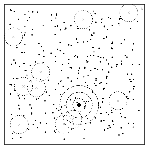
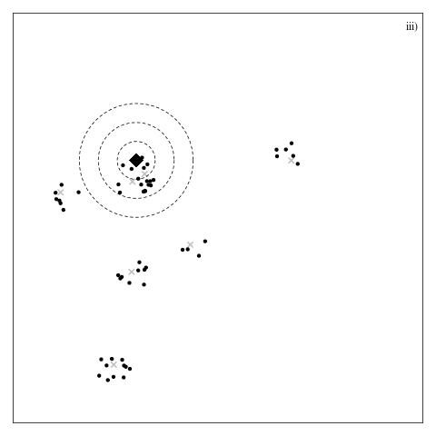
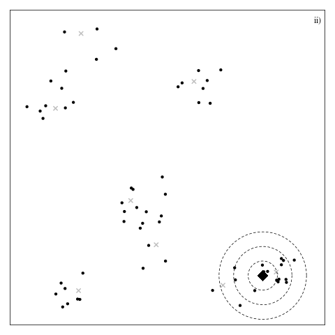
Figure 1: i) A simulated void processes in the unit square. With (unobserved) parent points (crosses) expunging daughters within a distance $R$ so that only the observed daughters remain (dots). The daughters are generated by a homogeneous Poisson process with densities $\lambda=300$. The number of parents simulated are IID following a Poisson distribution with expectation $D=10$. The distance beyond which daughters are safe from their parents is $R=0.075$. The dotted circles indicate the simulated voids. Noting an arbitrarily chosen daughter (encircled diamond) the distance between her and her sibling is clearly related to the proximity of a parent. The dashed circles show how the intensity of observed daughters changes for different distances $r$ away from an observed daughter. Plots ii) $\&$ iii): two simulated Neyman Scott point processes in the unit square; Thomas ii)), and Matérn iii)), with unobserved parent points (crosses) siring the observed daughters (dots). In each case parents are generated by a homogeneous Poisson process with intensity $D=7$. The number of daughters sired by each parent are IID following a Poisson distribution with expectation $\phi=8$. In each case $\gamma=0.05$. In the left hand plot daughters are dispersed around their parents due to a bivariate normal distribution, $\mathbf{N_{2}}(\mathbf{0},\boldsymbol{\sigma^{2}}\mathbf{I_{2}})$, where $\gamma=\sigma=0.05$, in the right hand plot daughters are uniformally distributed in a sphere with radius $R$ around their parents, hence $\gamma=R=0.05$.

3 Methodology

The approach taken here in order to estimate the parameter $\boldsymbol{\theta}$ for both the void and the cluster process discussed in Section 2 is based upon the derivation of the Palm intensity function. The Palm intensity function in each case, is parameterised by the vector $\boldsymbol{\theta}$, which reflects the structure of each process. Details of each Palm intensity (i.e., void and cluster process), are detailed in Sections 3.1.2 and 3.1.3 respectively. Derivation of these Palm intensities in d-dimensions is given in Appendix A. Our application requires only the Palm intensities in 2-dimensions, hence, only the 2-dimensional cases are discussed in the main body of this article.

3.1 Maximum Palm likelihood estimation

The likelihood for a Neyman-Scott point process is widely held to be intractable (Waagepetersen, 2007). However, an approach taken by Tanaka, Ogata and Stoyan (2008) shows that the pairwise distances can be approximated by a non-homogeneous Poisson point process, the intensity of which being proportional to the Palm intensity function. The likelihood for this approximating model is termed the Palm likelihood. Prokešová and Jensen (2013) show that such Palm likelihood estimators are consistent. In addition to using a Palm likelihood approach to estimate parameters of the Thomas and Matérn processes (Neyman Scott point processes) we also take such an approach to estimate the parameters of the void process.

3.1.1 The Palm intensity function

The Palm intensity, $\lambda(r;\boldsymbol{\theta})$, describes how the point density varies as a function of distance $r$ from an arbitrarily chosen point. Thus, the Palm intensity function returns the expected intensity of a point process at a distance $r$ from an arbitrarily chosen point. Figure 1 illustrates how the point density in a circle of radius $r$ centered at an arbitrary observed point, $b(x,r)$ (dashed circles), changes as $r$ increases. That is, at short distances the presence of a point suggests that there may exist a nearby sister. This is true for both the void and cluster processes, as, in the former case, conditional on observing a daughter the closest a possible parent can be is $R$. Therefore, any potential point is in danger if a parent exists in the circles of radius $R$ centered at the potential point minus the intersection of the two circles (for details see Appendix). In the latter case, by definition a clustered pattern infers that conditional on observing a daughter there is a high chance that another exists nearby.

The expected intensity of the point process at a distance $r$ from an arbitrarily chosen point depends on the parameters described in Section 2 above. The Palm intensity, $\lambda(r;\boldsymbol{\theta})$, can be defined as a function of the parameters $\theta$ that changes over distance $r$, decaying to the overall average intensity of the point process.

The following subsections derive the Palm intensity for a void process (Section 3.1.2), details the derivation of the Palm intensity for the Thomas process as Tanaka, Ogata and Stoyan (2008), and generalises this to the Matérn Palm intensity (Section 3.1.3).

3.1.2 Void process

Figure 1, plot i), illustrates that considering an observed daughter (the diamond), a potential nearby point is also likely to be safe. The Palm intensity of a void process is the product of the global point density of the pattern and the probability that a potential point at distance $r$ is in a safe area. The aforementioned probability is related to the geometry of the intersection between circles of common radius $R$ centered at the observed daughter (see Figure 1 plot i), encircled triangle) and a potential point. This is due to the expunging distance of parents, see Figure 1, plot i) dotted circles. Further details are given in Appendix A, and illustrated therein (see Figure 5).

The area of intersection between two 2-dimensional circles with a common radius R is given by $I(r)$, where,

$$I(r) =\pi\,R^{2}\,\text{I}\left(1-\left(\frac{r}{2R}\,\right)^{2};\frac{3}{2},\frac{1}{2}\right).$$ (1)

Here $\text{I}(z;a,b)=\frac{B(z;a,b)}{B(a,b)}$ is the regularised Beta function. The Palm intensity function is then derived as (see Appendix A),

$$\lambda(r;\boldsymbol{\theta}) =\lambda\,\text{exp}\left(-D\,\pi\,R^{2}\,\left[1-\text{I}\left(1-\left(\frac{r}{2R}\,\right)^{2};\frac{3}{2},\frac{1}{2}\right)\right]\right),$$ (2)

$$=\lambda\,\text{exp}\left(-D\,\pi\,R^{2}\,\left[1-\text{F}_{g(r)}\left(\frac{3}{2},\frac{1}{2}\right)\right]\right),$$

where $g(r)=1-\left(\frac{r}{2R}\,\right)^{2}$, and $\text{F}_{g(r)}(\cdot,\cdot)$ is the CDF of the Beta distribution. Note when $r=0$ $\Rightarrow$ $g(r)=1$ $\Rightarrow$ $\text{F}_{1}(\cdot,\cdot)=1$ $\Rightarrow$ $\lambda(0;\theta)=\lambda$, in addition when $r=2R$ $\Rightarrow$ $g(r)=0$ $\Rightarrow$ $\text{F}_{0}(\cdot,\cdot)=0$ $\Rightarrow$ $\lambda(0;\theta)=\lambda\,\text{exp}(-D\,\pi\,R^{2})$, due to the properties of the CDF.

Figure 2, plot i), shows both the empirical Palm intensity function (solid line), and the fitted Palm intensity (dashed line) for the simulated void process shown in Figure 1. The horizontal asymptote to which the Palm intensity decays is the global point density, the Palm intensity is a piece-wise continuous function with two sub-domains $(0,2R],[2R,\infty)$.

3.1.3 Neyman Scott point process

Under the conditions that (i) parent locations are realisations of a homogeneous Poisson process, (ii) the number of daughters sired by each parent are Poisson IID, and (iii) are dispersed due to a bivariate normal distribution with a variance-covariance matrix of any (positive-definite) form, Tanaka, Ogata and Stoyan (2008) derived the analytic Palm intensity for a modified Thomas process, as,

$$\lambda(r;\boldsymbol{\theta})=D\,\nu+\frac{\nu}{4\pi\sigma^{2}}\text{exp}\left(\frac{-r^{2}}{4\sigma^{2}}\right),$$ (3)

where $D\,\nu$ is the global point density. Thus, $\lambda(r;\boldsymbol{\theta})$ is the sum of the intensity of non-sibling points, $D\,\nu$, and a Gaussian function describing the intensity due to sibling points.

This Palm intensity function (Equation 3) has been extended to the d-dimensional case by Stevenson, Borchers and Fewster (In submission). Yet, as our application is in 2-dimensions we only discuss the 2-dimensional case here; thus, in general Equation (3) is given by,

$$\lambda(r;\boldsymbol{\theta}) =D\,\nu+\frac{\nu\,f_{y}(r;\gamma)}{2\,\pi\,r}.$$ (4)

The parameter $D$ is as discussed in Section 3.1.3 above. Letting $Y$ denote the distance between two randomly selected siblings (i.e., daughters sired by the same parent). Then $f_{y}(r;\gamma)$ is the PDF of this random variable, which is characterised by the parameter $\gamma$ pertaining to the form of distribution of daughters around their parents.

This PDF of the random variable, $Y$, refers to, in the case of the modified Thomas process, the distance between two normally distributed siblings. For example, in Equation 3,

$$f_{y}(r;\gamma)=\frac{r\>\text{exp}(-r^{2}/(4\gamma^{2}))}{2\>\gamma^{2}},$$ (5)

where, $\gamma=\sigma$, is the parameter describing the Gaussian dispersion of daughters around their parents.

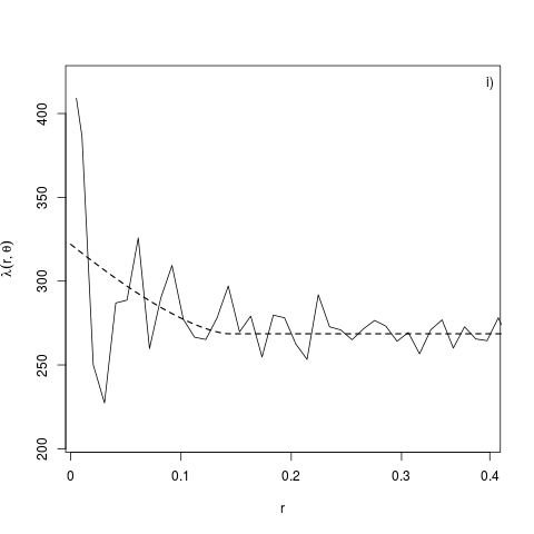
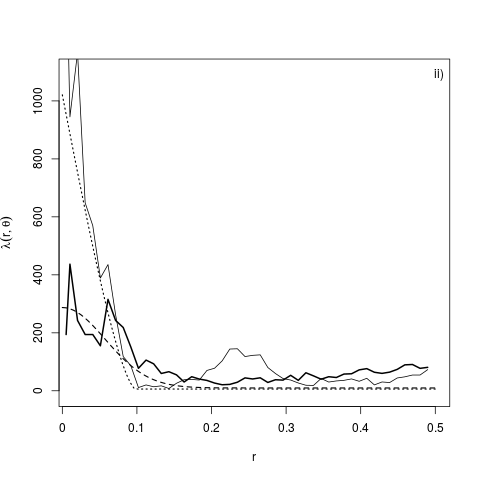
Figure 2: Both the empirical—solid lines—and fitted—dashed lines—Palm intensities for the simulated patterns above (see Figure 1). The Palm intensity for the void process is shown in plot i), it is evident that this function is a piece-wise continuous function with two sub-domains $(0,2R],[2R,\inf)$. The Palm intensities for both the simulated Neyman Scott point processes are shown in plot ii), where the Matérn cluster process (thinner solid line), decays at a much steeper rate, due again to it being a piece-wise continuous function with two sub-domains $(0,2R],[2R,\inf)$. In each case the Palm intensities decay to the global point density of the process.

In considering the Matérn process, we follow the same methodology in deriving the Palm intensity function of the aforementioned process. The random variable $Y$, is now the distance between two siblings that are uniformally distributed in a 2-dimensional sphere of radius $R$ around their parents. The PDF of $Y$ is shown below (Tu and Fischbach, 2002), using both the hyper-geometric function and integral representation respectively,

$$f_{y}(r;R) =\frac{4}{B(\frac{3}{2},\frac{1}{2})}\,\frac{r}{R^{3}}\times\left[{}_{2}F_{1}\left(\frac{1}{2},-\frac{1}{2},\frac{3}{2},1\right)\,R-{}_{2}F_{1}\left(\frac{1}{2},-\frac{1}{2},\frac{3}{2},\frac{r^{2}}{4\,R^{2}}\right)\,\frac{r}{2}\right],$$ (6)

$$=\frac{4\,r\,\int^{R}_{\frac{r}{2}}(R^{2}-x^{2})^{\frac{1}{2}}dx}{B(\frac{3}{2},\frac{1}{2})\,R^{4}}.$$

Here $B(\cdot,\cdot)$ denotes the beta function, and ${}_{2}F_{1}(\cdot,\cdot,\cdot,\cdot)$ the hyper-geometric function.

Figure 2, plot ii) shows the Palm intensities for the simulated Neyman Scott point processes in Figure 1 (the Thomas process, plot ii); Matérn process, plot iii)). The solid lines are the empirical palm intensities for each process (Matérn process—thinner line, Thomas process—thicker line). Dashed lines (Matérn process—short dash, Thomas process—long dash) are the respective fitted Palm intensities. Both simulated processes in Figure 1, plots ii) and iii), were simulated with the same parameter values $\boldsymbol{\theta}=(7,8,0.05)$. Hence, the Palm intensities in each case decay to the same asymptote, the global point density $D\nu$. The Palm intensity of the Matérn process is initially a lot higher, and decays at a much faster rate to that of the Thomas process with the same parameterisation; this as, the parameter $\gamma$ controls the dispersion of daughters around their parents (the radius of dispersion in a Matérn process and the spread in a Thomas process). For the Matérn process $\gamma$ is a hard boundary which induces a much higher intensity at shorter distances. Also of note is the similarity between the Palm intensity of the Matérn process and the void process, namely the shape (piece-wise continuous with two sub-domains $(0,2R],[2R,\infty)$), and this is again due to the geometry of the structure.

3.2 The Palm likelihood

Taking an approximate-likelihood approach, the estimator for $\boldsymbol{\theta}$ is given by

$$\hat{\boldsymbol{\theta}}=\text{arg}\,\text{max}_{\boldsymbol{\theta}}\,L(\boldsymbol{\theta};\mathbf{r}),$$

which is evaluated through the numerical maximisation of $\text{log}(L(\boldsymbol{\theta};\mathbf{r}))$ with respect to $\boldsymbol{\theta}$. Here, $L(\boldsymbol{\theta};\mathbf{r})$ is termed the Palm likelihood and given by,

$$L(\boldsymbol{\theta};\mathbf{r})=\left(\prod n\,\lambda(r;\boldsymbol{\theta})\right)\,\text{exp}\left(-n\int_{0}^{t}\lambda(r;\boldsymbol{\theta})\,2\,\pi\,r\>\text{d}r\right),$$ (7)

where the integral is a volume of $2$ dimensions around the intensity axis. Below, the integral is simplified for each process discussed herein, providing a closed-form Palm likelihood function in each case. This results in an objective function that is very computationally efficient to compute.

• Void process The integral for the void process is intractable as it contains the CDF of a Beta distribution, however it can be simplified.

  $$\int_{0}^{t}\lambda_{o}(r;\boldsymbol{\theta})\,2\,\pi\,r\>\text{d}r=\lambda\,2\,\pi\,\text{exp}\left(-D\,\pi\,r^{2}\>\right)\,\int_{0}^{t}\text{exp}\left(D\,\pi\,r^{2}\>\text{F}_{g(r)}\left(1,\frac{1}{2}\right)\right)\,r\,\text{d}r.$$

  Refer to Appendix A for a derivation of these.

• Neyman Scott point processes The integral simplifies as,

  $$\int_{0}^{t}\lambda_{o}(r;\boldsymbol{\theta})\,2\,\pi\,r\>\text{d}r=D\,\nu+\nu\>\,F_{y}(t;\gamma),$$

  where $F_{y}(t;\gamma)$ is the CDF of the distance between two randomly distributed siblings. Below are each $F_{y}(t;\gamma)$ for each case of the Neyman Scott point process.

  • Matérn cluster process

    $$F_{y}(t;R)=\frac{t^{2}}{R^{2}}\left(1-\frac{B_{\alpha}\left(\frac{1}{2},\frac{3}{2}\right)}{B\left(\frac{1}{2},\frac{3}{2}\right)}\right)+4\,\frac{B_{\alpha}\left(\frac{3}{2},\frac{3}{2}\right)}{B\left(\frac{1}{2},\frac{3}{2}\right)},$$

    where $B_{\alpha}(\cdot,\cdot)$ and $B(\cdot,\cdot)$ are the incomplete beta function and the beta function respectively. That is $B(\alpha;a,b)=\int_{0}^{\alpha}u^{(a-1)}(1-u)^{(b-1)}du$, and for $\alpha=1$ $B(\alpha;a,b)=B(a,b)$. The derivation of these equations is detailed in Appendix A.

  • Thomas cluster process Letting $q=\sigma_{\chi}\sqrt{2}$, which is strictly monotonic. Then, showing the derivation of Stevenson, Borchers and Fewster (In submission),

    $$F_{q}(q;\sigma)=P\left(1,\frac{4q^{2}}{\sigma^{2}}\right)$$

    where $P(\cdot,\cdot)$ is the regularised gamma function.

4 Application to histopathology data

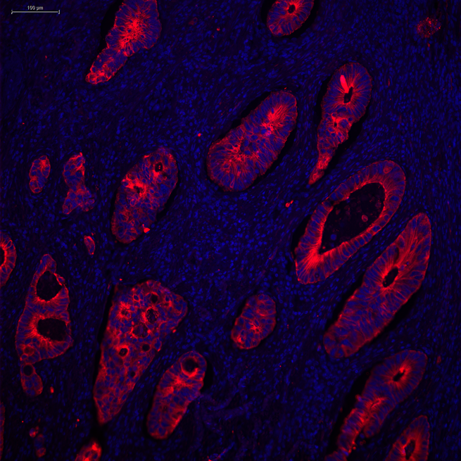
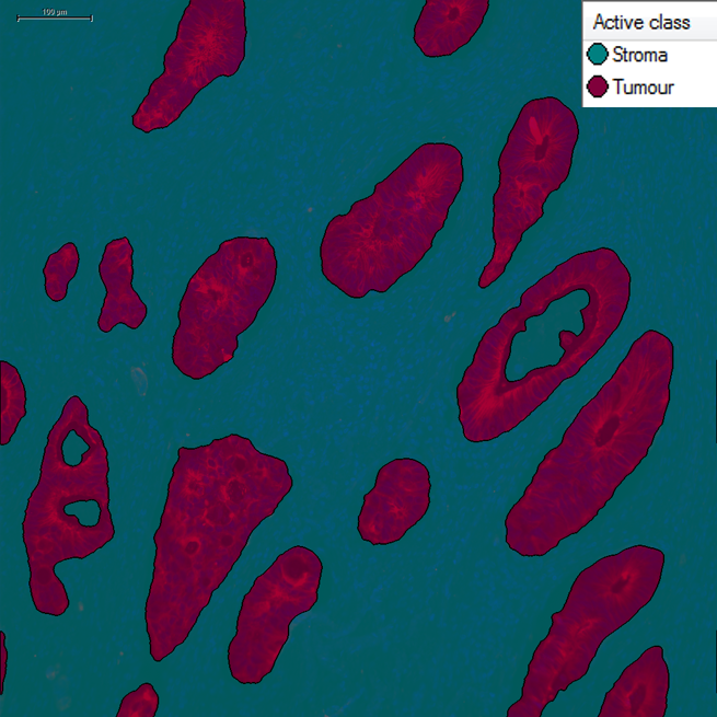
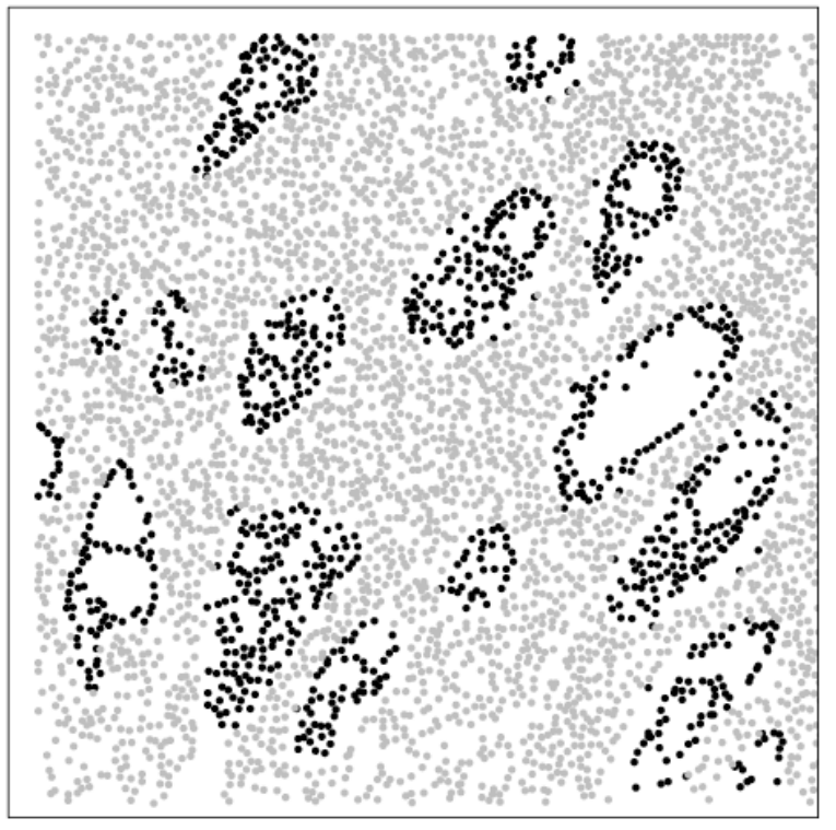
Figure 3: Illustration of the image analysis of one patient’s slide which enables the pinpointing of nuclei. Left: Composite immunofluorescence digital image showing Tumour (red), Stroma (green) and all nuclei (blue). Middle: Image analysis mask overlay from automatic machine learnt segmentation of the digital image. Tumour (purple), stroma (turquoise), necrosis (yellow). Right: Point pattern formed by the nuclei of the tumour (black) and stroma (grey) cells shown in the previous two images.

Our data set pertains to 42 patients drawn from a wider data set of a pan-Scotland cohort of patients with CRC (see Caie et al. (2014) for a full description of our data set). In this subset of data, 23 patients died from CRC, and 19 survived. Each patient had up to 15 images from the invasive front of the tissue section processed by an automatic imaging algorithm described in Caie and Harrison (2016). In summary, distinct regions in the digitised tissue section were first divided into four types through machine learning: (i) tumour, (ii) stroma, (iii) necrosis/lumen and (iv) no tissue. The positions of all cell nuclei were automatically identified (see Caie and Harrison (2016)) and exported by the image analysis software (Definiens, 2000), see Figure 3. The centres of each nucleus provide us with our point patterns of tumour and stroma cells. In Section 4.1 we consider tumour cells and stroma cells as separate void processes and seek to differentiate tissue sections based on patient survival. Then, in Section 4.2 we consider both tumour and stroma cells, fitting a Thomas process to each and using a graph theoretic approach to inform analysis of the spatial interaction between the cell types. In both these sections hierarchical bootstrap procedures were carried out following estimation of the associated parameters. A hierarchical bootstrap is required due to there being multiple images per patient. In particular, a patient is chosen at random, the data is subset, and then resampled. Then, the bootstrap is repeated a chosen number of times, in this case 1000. Finally, in Section 4.3 we assess the predictive performance of each void and Thomas process through cross validation.

4.1 Void processes for tumour and stroma cells

Recall that a void in the context of spatial point patterns is a region that contains no point where, given the general structure of the data, points may be expected. This section assumes that each of the separate point patterns formed by tumour and stroma nuclei are realisations of void processes, and so point patterns characterise the gaps in the distribution of nuclei. In this way, the void process describing the tumour cell point pattern reflects the patterning of stroma cells and vice versa; note the void processes also reflect the less frequently occurring regions of necrosis/lumen and no tissue.

4.1.1 Results

Following estimation of $\theta=(R,D,\gamma)$ (for each of the stroma and tumour patterns) as per the methodology described above, a hierarchical bootstrap procedure (as detailed above), to account for patient effect, using 1000 simulations was carried out using the estimated parameters of interest for each patient group (i.e., those patients who were alive and those who died). Table 1 contains the medians and bootstrapped quantities of the distributions of the parent densities, $\hat{D}$, and void radii, $\hat{R}$, pertaining to each point pattern (subscripts $t$ and $s$ refer to tumour and stroma patterns respectively). Here the superscripts $d$ and $a$ refer to whether the patients were dead or alive at follow-up respectively. The results in Table 1 reveal three findings in reference to the tumour void patterns:

1. There is no overlap between the patients who lived and the patients who died in the distribution of void densities;

2. The values of the parent densities are lower for patients who lived than for patients who died;

3. The estimated void radii pertaining to patients who lived and died are similar.

When considering the stroma void patterns, there are no clear differences between patient groups for density or radii.

Table 1: The medians and bootstrapped quantities (based on 1000 simulations) of the distributions of the parent densities and void radii for each of the point patterns formed by both tumour and stroma cells (subscript $t$ and $s$ respectively) of either patients who lived or died (superscripts $a$ and $d$ respectively) assuming a void process.

	Median	2.5% Quantile	97.5%Quantile
$\hat{D}_{t}^{a}$	8.6404	7.6931	9.4268
$\hat{D}_{t}^{d}$	15.4272	12.7820	18.2618
$\hat{R}_{t}^{a}$	0.2142	0.1977	0.2305
$\hat{R}_{t}^{d}$	0.2152	0.1858	0.2417
$\hat{D}_{s}^{a}$	6.0304	5.3665	7.9776
$\hat{D}_{s}^{d}$	5.4828	5.0402	6.5505
$\hat{R}_{s}^{a}$	0.2097	0.1929	0.2229
$\hat{R}_{s}^{d}$	0.2149	0.1976	0.2296

4.2 Thomas processes for tumour and stroma cells

In the context of histopathology, a Neyman Scott point process can be thought of as a process giving raise to the clustering of cells within the tissue. Therefore, we assume that the distribution of cells within each of the tumour and the stroma are assumed to be realisations of two different Neyman Scott point process. Observed cells are daughters and we seek to infer the unobserved parents. Parents thus represent some abstracted developmental process that led to the observed arrangement of daughter cells within the tissue.

4.2.1 Framework and Results

In order to fit Thomas processes to each pattern formed by tumour and stroma nuclei, we use the R package nspp (Stevenson, 2015), to estimate $\boldsymbol{\theta}$ in each case. In order to fit the models it is required that we indicate the maximum distance we would expect a daughter to be from its parent, hence a reflection of the inter-cellular structure. This information is not supplied heuristically, but inferred from the use of a class cover catch digraph (CCCD) (details are given in Appendix B). The estimation of $\boldsymbol{\theta}=(D,\phi,\gamma)$ leads to the analytic derivation of daughter density, $\delta$.

As above, in order not to make any distributional assumptions, a hierarchical bootstrap (to account for patient effect) procedure is carried out using the estimated parameters of interest for each pattern. Table 2 contains the medians and bootstrapped quantities of the distributions of both the parent, $\hat{D}_{\cdot}^{\cdot}$, and daughter, $\hat{\delta}_{\cdot}^{\cdot}$, densities along with dispersion parameters—$\hat{\sigma}_{\cdot}^{\cdot}$, pertaining to each tumour and stroma point pattern. The results in Table 2 reveal 6 key findings:

1. The values of both parent and daughter densities are higher for patients who lived than for patients who died in both stroma and tumour data;

2. The differences in the distribution of both parent and daughter densities between patients who lived and patients who died are larger in the stroma data than in the tumour data;

3. For tumour data, there is no overlap in the distributions between patients who lived and patients who died in the daughter densities, while parent density distributions overlap;

4. For stroma data, there is no overlap in the distributions between patients who lived and patients who died in the parent or daughter densities;

5. For dispersion, there is no overlap in the distributions between patients who lived and patients who died in the daughter densities for stroma data, while distributions overlap in the tumour data;

6. For the stroma data, the dispersion is higher in patients who lived than patients who died.

For the distributions that did not overlap, the lowest value from one group is larger than the highest value in the other, thus indicating that the parameter estimates from a patient’s slides are likely to be a good predictor for whether or not they survived. We formally assess the predictive power of this classifier into the following section.

Table 2: The medians and bootstrapped quantiles (based on 1000 simulations) of the distributions of both the daughter, $\hat{\delta}_{\cdot}^{\cdot}$, and parent, $\hat{D}_{\cdot}^{\cdot}$, densities along with dispersion parameters, $\hat{\sigma}_{\cdot}^{\cdot}$, for each of the point patterns formed by tumour and stroma nuclei—subscript $t$ and $s$ respectively—of either patients who lived or died—superscript $a$ and $d$ respectively, assuming a Thomas cluster process.

	Median	2.5 % Quantile	97.5 % Quantile
$\hat{\delta}_{t}^{a}$	2048.7671	1577.7571	2447.5904
$\hat{\delta}_{t}^{d}$	1249.8016	962.0058	1550.2289
$\hat{\delta}_{s}^{a}$	3005.7470	1685.8138	4100.7619
$\hat{\delta}_{s}^{d}$	1057.6313	740.6736	1564.4209
$\hat{D}_{t}^{a}$	91.6861	63.8080	273.3591
$\hat{D}_{t}^{d}$	65.3319	47.2276	89.9136
$\hat{D}_{s}^{a}$	89.7333	39.1060	147.8126
$\hat{D}_{s}^{d}$	20.2366	9.2333	40.8440
$\hat{\sigma}_{t}^{a}$	0.0262	0.0198	0.0339
$\hat{\sigma}_{t}^{d}$	0.0253	0.0215	0.0287
$\hat{\sigma}_{s}^{a}$	0.0335	0.0264	0.0404
$\hat{\sigma}_{s}^{d}$	0.0634	0.0463	0.0936

4.3 Cross validation

We propose using the parameter estimates of the point processes discussed above to predict patients’ outcomes. We assess the predictive power of each of these classifiers (estimates from each point process) using receiver operating characteristic (ROC) curves. Specifically, the means of each classifier were calculated per patient for use in a logistic regression (in predicting patient outcome). Figure 4 shows the ROC curves for each classifier along with the associated area under the ROC curve (AUROC) and leave one out cross validation (CV) scores. An AUROC score is a measure of classifier performance. To put our calculated AUROC scores in context, it should be noted that a score of 0.5 would indicate that our classifier does no better than random at distinguishing between patients who died or survived. In addition, a AUROC score of 1 would indicate perfect separation between each patient group (i.e., no overlap in distribution of our classifiers). The CV scores are an estimate of the test error for the logistic regression models using each classifier. From Figure 4, notably, void density of the tumour pattern is the best predictor for patient outcome (AUROC of 0.84 and CV of 0.19). Further, when considering the AUROC scores, daughter density of the assumed Thomas process for the stroma patterns is considered the second best predictor. To asses goodness of fit of the assumed processes we compare the empty space function of the observed data to those patterns simulated with estimated parameter values. For further details see Appendix D where this concept is illustrated using the pattern shown in Figure 3.

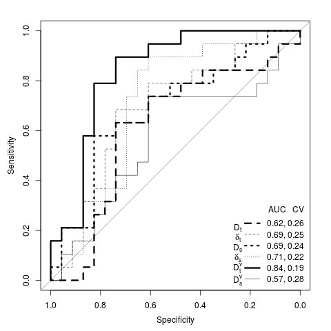
Figure 4: Plot of the ROC curves for each of the measures per patient. Legend includes the AUROC (area under the ROC curve) score for each curve and the CV (leave one out cross validation) score for each classifier (i.e., $D_{\cdot}$, $\delta_{\cdot}$, and $D^{v}_{\cdot}$ parent, daughter densities of a Thomas process and void density of a void process respectively for tumour and stroma patterns (subscripts $t$ and $s$ respectively))

5 Discussion

Our void process analysis of gaps in tumour or stroma cells reflects the stroma or tumour cell patterning, respectively as explained in Section 4.1. The tumour cell void patterning is the most discriminatory and has the best predictive power: there is a clear separation in parent densities (rows 1 and 2, Table 1); the best patient outcome classifier is based on the gaps in tumour cells (AUROC=0.82, thick solid line of Figure 4). In contrast, the void process describing stroma cell gaps is the least discriminatory and has the worst predictive power: there is no clear separation in parent densities (rows 5 and 6, Table 1); the classifier based on stroma gaps has an AUROC value approaching random (0.57, thin solid line of Figure 4). Results show that stroma patterning is a better indicator of patient outcome than tumour patterning.

Notably, and in the context of this marked difference in performance, the radii of the voids are very similar in both tumour and stroma patterns for all patients, irrespective of whether they lived or died. This observation combined with the result that parent density is lower in patients that lived than patients that died means that there are fewer voids in patients who lived and those voids are similar in size to those observed in patients who died.

Our analysis using cluster point processes further supports the observation that stroma patterning is more informative than tumour patterning. Parent and daughter densities are clearly more distinct between patients who lived and patients who died for the stroma data than for the tumour data, with densities being lower in patients who died. This finding is also reflected in the cross-validation results, where a classifier based on the Thomas process daughter density results in the second best AUROC (0.71, thin dotted line of Figure 4). We also observe a difference in the dispersion data: stroma clusters are more dispersed in patients who lived than in patients who died; there is no difference between patient groups in the tumour data. Thus stroma cells patterns have fewer, larger and more dispersed clusters in patients who lived than in patients that died.

These observations emerge from our unbiased data analysis and can be linked to tumour-scale patterns in patients. High tumour budding is found in patients with an infiltrative growth pattern: finger-like protrousions invading widely across the stroma and thus forming large gaps between the cancer protrusions. Both tumour budding and infiltrative growth pattern would be reflective of the tumour cell void patterning described herein. In contrast, low tumour budding, or a pushing border growth pattern, described as a solid tumour mass with little stroma existing between cells, has been correlated with good outcome (Zlobec et al., 2009). Although the literature reports these features to be significantly associated with disease survival, the lack of consensus on quantification method, and observer variability has led to their exclusion from clinical guidelines (Karamitopoulou et al., 2015). Our novel method provides a standardised methodology that accurately describes and reports on tumour cell distribution patterns which significantly correlate with patient outcome in CRC and that negates observer variability.

Our method points to the importance of stromal features in predicting patient outcome. The relevance of stroma patterns to patient outcome has also been reported in breast cancer (Beck, 2011), where the most differentiating measure was a measure of fragmentation: patients with good outcomes had tissue that had larger contiguous regions of stroma interspersed with larger epithelial regions; this patterning is reflected in our nuclei-level analysis. More broadly, this work reflects a growing interest in the use of analytical techniques more commonly associated with ecology in recognition of the importance of both spatial structure and spatial variations within that structure. For example, Nawaz et al. (2015) observed that both the abundance of immune cells and their spatial variation within the tumour are important factors in patient outcome. Further, in a recent review of spatial heterogeneity in cancers, Heindl, Nawaz and Yuan (2015) set out the importance of such ecological views of cellular patterns and the relevance of spatial statistics in describing succinctly those patterns. Moreover they suggest the combined exploration of spatial patterns of cells and cellular characteristics.

Here, we have presented a novel application of spatial statistics to capture the spatial arrangement of cells through both void processes and clustered processes. This work aligns with this growing recognition of the value of analytical methods more typical in ecological contexts to understand the ecology of cancer. In the future, we will build on our initial analysis by refining our treatment of individual cells, stratifying individual cells further by biological and/ or physical measurements to explore more complex questions that point at specific mechanisms of disease progression.

Appendix A The Palm intensity function

This appendix derives the d-dimensional Palm intensity functions for both the void, and Matérn process discussed in this article. The d-dimensional Palm intensity for the modified Thomas process is derived by Stevenson, Borchers and Fewster (In submission). Our application considers only the 2-dimensional case; therefore, the article only provides details of the Palm intensities and likelihoods in 2-dimensions. This appendix generalises this to consider d-dimensions. Due to this we now consider the volume of hyper-spheres, and not the area of circles.

A.1 A $d$-dimensional void point process

The probability of a potential point being safe is related to the geometry of the intersection between hyper-spheres of common radius $R$ centered at the observed daughter (see Figure 1, plot i) encircled triangle) and a potential point, due to the expunging distance of parents (see Figure 1, plot i) dotted circles). This geometry is illustrated in Figure 5.

Figure 5: Figure showing the intersection of two spheres, in 2D, of radius $R$. The closed plotting character represents an observed daughter, the open plotting character represents a possible point. We know that there cannot exist a parent within distance $R$ of the observed daughter, therefore the intersection $I(r)$ is the area within which any possible point is “safe”. To ascertain the intersection between two hyper-spheres of common radius $R$ the radius of the hyper-spherical caps, $R\,\text{sin}(\theta)$, and the height of the hyper-spherical caps $R\,\text{cos}(\theta)$ is required, where $\theta$ is the colatitude angle. Thus, the volume of intersection only depends on the radii of the hyper-spheres as well as the distance between their centers $r$, see Equation 8.

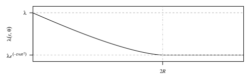
Figure 6: The functional form of the Palm intensity for the void process in 2 dimensions. The horizontal asymptote is given by $\lambda\,\text{exp}(-D\pi R^{2})$, which is the value that $\lambda_{0}(r)$ decays to for values of $r\geq 2\,R$. The Palm intensity at $r=0$ is simply $\lambda$, as for $r=0$ $g(r)=1$ in Equation 2, thus the exponential becomes $1$. At the value $r=2R$ the volume of intersection between the spheres encircling an observed daughter and a potential point of radius $R$ is zero, thus the contribution from the CDF of the Beta distribution to $\lambda(r;\theta)$ is zero.

The volume of intersection, $I(r)$ in Figure 5, between two d-dimensional spheres with a common radius R is derived as in Li (2011). To calculate $I(r)$, the integrand of the volume of a $\text{d}-1$ sphere of radius $R\,\text{sin}(\boldsymbol{\theta})$ with height $R\,\text{cos}(\boldsymbol{\theta})$ is required. As the hyper-spheres are of common radius, $R$, $I(r)$ is simply just twice this volume. Hence;

$$I^{\text{d}}(r) =2\times\int_{0}^{\phi}v^{\text{d}-1}(R\text{sin}\boldsymbol{\theta})\,\text{d}R\text{cos}\boldsymbol{\theta},$$ (8)

$$=2\times\int_{0}^{\phi}v^{\text{d}-1}(R\text{sin}\boldsymbol{\theta})R\text{sin}\boldsymbol{\theta}\,\text{d}\boldsymbol{\theta},$$

$$=2\times\frac{\pi^{\frac{\text{d}-1}{2}}}{\Gamma(\frac{\text{d}-1}{2}+1)}\,R^{\text{d}}\int_{o}^{\phi}\text{sin}^{\text{d}}\boldsymbol{\theta}\,\text{d}\boldsymbol{\theta},$$

$$=2\times\frac{\pi^{\frac{\text{d}-1}{2}}}{\Gamma(\frac{\text{d}-1}{2}+1)}\,R^{\text{d}}\,\text{J}_{d}(\phi),$$

$$=\frac{\pi^{\frac{\text{d}-1}{2}}}{\Gamma(\frac{\text{d}-1}{2}+1)}\,R^{\text{d}}\,B\left(\frac{\text{d}+1}{2},\frac{1}{2}\right)\,\text{I}\left(\text{sin}^{2}\phi;\frac{\text{d}+1}{2},\frac{1}{2}\right),$$

$$=v^{\text{d}}(R)\,\text{I}\left(\text{sin}^{2}\phi;\frac{\text{d}+1}{2},\frac{1}{2}\right),$$

$$=v^{\text{d}}(R)\,\text{I}\left(1-\left(\frac{r}{2R}\,\right)^{2};\frac{\text{d}+1}{2},\frac{1}{2}\right),$$

noting that $B(a,b)=\frac{\Gamma(a)\,\Gamma(b)}{\Gamma(a+b)}$, $\Gamma\left(\frac{1}{2}\right)=\sqrt{\pi}$, and that $(R\,\text{cos}\boldsymbol{\theta})^{2}+(R\,\text{sin}\boldsymbol{\theta})^{2}=R^{2}\rightarrow(\text{sin}\,\boldsymbol{\theta})^{2}=1-(\text{cos}\boldsymbol{\theta})^{2}$ and using the cosine rule leads to $\text{cos}\,\boldsymbol{\theta}=\frac{r^{2}+R^{2}-R^{2}}{2\,r\,R}=\frac{r}{2\,R}$. Also $\text{I}(z;a,b)=\frac{B(z;a,b)}{B(a,b)}$ is the regularised Beta function.

The Palm intensity of the void process then becomes;

$$\lambda_{0}(r) =\lambda\,\text{exp}\left(-D\,v^{\text{d}}(R)\left[1-\text{I}\left(1-\left(\frac{r}{2R}\,\right)^{2};\frac{\text{d}+1}{2},\frac{1}{2}\right)\right]\right),$$ (9)

$$=\lambda\,\text{exp}\left(-D\,v^{\text{d}}(R)\left[1-\text{F}_{g(r)}\left(\frac{\text{d}+1}{2},\frac{1}{2}\right)\right]\right),$$

where $g(r)=1-\left(\frac{r}{2R}\,\right)^{2}$, and $\text{F}_{g(r)}(\cdot,\cdot)$ is the CDF of the Beta distribution. Thus; when $r=0$ $\Rightarrow$ $g(r)=1$ $\Rightarrow$ $\text{F}_{1}(\cdot,\cdot)=1$ $\Rightarrow$ $\lambda_{0}(0)=\lambda$, in addition when $r=2R$ $\Rightarrow$ $g(r)=0$ $\Rightarrow$ $\text{F}_{0}(\cdot,\cdot)=0$ $\Rightarrow$ $\lambda_{0}(0)=\lambda\,\text{exp}(-D\,v_{\text{d}}(R))$, due to the properties of the CDF. The functional form of this Palm intensity is shown in Figure 6. Substituting d$=2$ into Equation (9) would lead to the Palm intensity given in Equation (2).

A.2 A $d$-dimensional Matérn point process

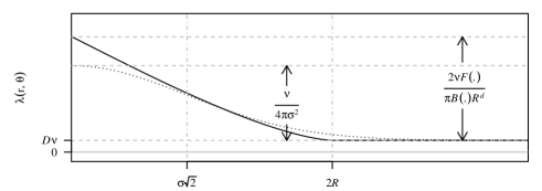
Figure 7: The functional form of the Palm intensity for both the Matérn (solid curve) and Thomas (dotted curve) variants of the Neyman Scott point process in 2 dimensions. The horizontal asymptote is given by $D\,\nu$ for both processes. The difference between the horizontal asymptote and the $y-intercept$ is given by $\nu/(4\,\pi\,\sigma^{2})$ for the Thomas process, and $2\,\nu\,F(\cdot)/(\pi\,B(\cdot)\,R^{2})$ for the Matérn process. Here $F(\cdot)={}_{2}F_{1}\left(\frac{1}{2},\frac{1}{2}-\frac{\text{d}}{2},\frac{3}{2},1\right)$ denotes the hyper-geometric function, and $B(\cdot)=B(\frac{3}{2},\frac{1}{2})$ denotes the beta function. The point of inflection of the Gaussian term for the Thomas process is given by $\sigma\,\sqrt{(}2)$, for the Matérn process $2\,R$ is the point at which the Palm intensity decays to the horizontal asymptote.

Daughters of a Matérn process are uniformally distributed around their parents. The parameter $\gamma$ in Equation 4 refers to the radius of the sphere centered at a selected parent outwith which we do not observed sired daughters. Figure 1 illustrates the two types of Neyman Scott point processes simulated with the same value of $\gamma$. Thus, for the same value of $\gamma$ clearly the Palm intensity function for the Matérn process is initially much higher, and decays at a much faster rate to the horizontal asymptote, $D\,\nu$. As illustrated in Figure 7, letting $\gamma=R$, $\lambda(r;\boldsymbol{\theta})$ is a continuous piece-wise monotonic function of two sub-domains, $[0,2R]$ and $[2R,\infty)$. The common endpoint of the sub-domains, $2R$, relates to the structure of the Matérn process, that is, the distance between two sibling daughters cannot be more than the diameter, $2R$, of a sphere centered at an unobserved parent away from one another. Thus, the probability of observing a sibling at a distance $r$ from an arbitrarily chosen daughter pertains to the intersection of the hyper-spheres centered at these points, $b(x,R)\cap b(y,R),{x\neq y}\in N$, where $N$ is the point pattern. Clearly when the distance between these points, $r\geq 2R$ then $b(x,R)\cap b(y,R)=0$.

The d-dimensional version of Equation 6 is given by,

$$f_{y}^{\text{d}}(r;R) =\frac{2\,\text{d}}{B(\frac{\text{d}}{2}+\frac{1}{2},\frac{1}{2})}\,\frac{r^{\text{d}-1}}{R^{\text{d}+1}}\,\left[{}_{2}F_{1}\left(\frac{1}{2},\frac{1}{2}-\frac{\text{d}}{2},\frac{3}{2},1\right)\,R-{}_{2}F_{1}\left(\frac{1}{2},\frac{1}{2}-\frac{\text{d}}{2},\frac{3}{2},\frac{r^{2}}{4\,R^{2}}\right)\,\frac{r}{2}\right],$$ (10)

$$=\frac{2\,\text{d}\,r^{\text{d}-1}\,\int^{R}_{\frac{r}{2}}(R^{2}-x^{2})^{\frac{\text{d}-1}{2}}dx}{B(\frac{\text{d}}{2}+\frac{1}{2},\frac{1}{2})\,R^{2\,\text{d}}}.$$

Here $B(\cdot,\cdot)$ denotes the beta function, and ${}_{2}F_{1}(\cdot,\cdot,\cdot,\cdot)$ the hyper-geometric function.

Below we show how this PDF reduces in $d=2$ and $d=3$ to forms equivalent to the PDFs of the distances between two randomly selected siblings given by Illian et al. (2008, p. 376) in the respective dimensions.

$\bullet$ for $\text{d}=2$ It should be noted that,

$$\int^{R}_{\frac{r}{2}}(R^{2}-x^{2})^{\frac{\text{d}-1}{2}}dx =\int^{R}_{\frac{r}{2}}(R^{2}-x^{2})^{\frac{1}{2}}dx$$

$$=\frac{1}{8}\left(4\,R^{2}\,\text{sec}^{-1}\left(\frac{2\,R}{r}\right)-r\,\sqrt{4\,R^{2}-r^{2}}\right).$$

therefore,

$$\frac{2\,\text{d}\,r^{\text{d}-1}\,\int^{R}_{\frac{r}{2}}(R^{2}-x^{2})^{\frac{\text{d}-1}{2}}dx}{B(\frac{\text{d}}{2}+\frac{1}{2},\frac{1}{2})\,R^{2\,\text{d}}} =\frac{4\,r\,\int^{R}_{\frac{r}{2}}(R^{2}-x^{2})^{\frac{1}{2}}dx}{B(\frac{\text{3}}{2},\frac{1}{2})\,R^{4}}$$

$$=\frac{r\,\Gamma(2)}{\frac{1}{2}\sqrt{\pi}^{2}\,R^{4}\,2}\left(4\,R^{2}\,\text{sec}^{-1}\left(\frac{2\,R}{r}\right)-r\,\sqrt{4\,R^{2}-r^{2}}\right)$$

$$=\frac{r}{\pi\,R^{4}}\,\left(4\,R^{2}\,\text{sec}^{-1}\left(\frac{2\,R}{r}\right)-r\,\sqrt{4\,R^{2}-r^{2}}\right)$$

$$=\frac{r}{\pi\,R^{4}}\,\left(4\,R^{2}\,\text{cos}^{-1}\left(\frac{r}{2\,R}\right)-r\,\sqrt{4\,R^{2}-r^{2}}\right),$$

noting that $\text{sec}^{-1}(x)=\text{cos}^{-1}\left(\frac{1}{x}\right)$, and as $B(\frac{\text{3}}{2},\frac{1}{2})=\frac{\Gamma(\frac{3}{2})\,\Gamma(\frac{1}{2})}{\Gamma(2)}$, recalling that $\Gamma(\frac{3}{2})=\frac{1}{2}\sqrt{\pi}$, $\Gamma(\frac{1}{2})=\sqrt{\pi}$, and $\Gamma(2)=1$.

$\bullet$for $\text{d}=3$ It should be noted that,

$$\int^{R}_{\frac{r}{2}}(R^{2}-x^{2})^{\frac{\text{d}-1}{2}}dx =\int^{R}_{\frac{r}{2}}(R^{2}-x^{2})dx$$

$$=\frac{1}{24}\,\left(r-2\,R\right)^{2}\,\left(r+4\,R\right).$$

therefore,

$$\frac{2\,\text{d}\,r^{\text{d}-1}\,\int^{R}_{\frac{r}{2}}(R^{2}-x^{2})^{\frac{\text{d}-1}{2}}dx}{B(\frac{\text{d}}{2}+\frac{1}{2},\frac{1}{2})\,R^{2\,\text{d}}} =\frac{6\,r^{2}\,\int^{R}_{\frac{r}{2}}(R^{2}-x^{2})dx}{B(2,\frac{1}{2})\,R^{6}}$$

$$=\frac{6\,r^{2}}{24\,B(2,\frac{1}{2})\,R^{6}}\,\left(r-2\,R\right)^{2}\,\left(r+4\,R\right),$$

$$=\frac{r^{2}\,\Gamma(\frac{5}{2})}{4\,R^{6}\,\Gamma(2)\,\Gamma(\frac{1}{2})}\,\left(r-2\,R\right)^{2}\,\left(r+4\,R\right)$$

$$=\frac{r^{2}\,\frac{3}{4}\,\sqrt{\pi}}{4\,R^{6}\,\sqrt{\pi}}\,\left(r-2\,R\right)^{2}\,\left(r+4\,R\right)$$

$$=\frac{3\,r^{2}}{16\,R^{6}}\,\left(r-2\,R\right)^{2}\,\left(r+4\,R\right)$$

$$=\frac{3\,r^{2}}{16\,R^{6}}\left(R-\frac{r}{2}\right)^{2}\left(2\,R+\frac{r}{2}\right).$$

noting that $\Gamma(\frac{5}{2})=\frac{3}{4}\sqrt{\pi}$, $\Gamma(\frac{1}{2})=\sqrt{\pi}$, and $\Gamma(2)=1$.

Upon substitution of the PDF, given by Equation 10, into the Palm intensity function, given by Equation 4, as in the case of the modified Thomas process above simplifications occur which circumvent numerical instability in $\lambda(r;\boldsymbol{\theta})$ at $r=0$ as both the numerator and denominator in the second term contain the term $r^{d-1}$. Thus,

$$\lambda(r;\boldsymbol{\theta}) =D\,E_{c}(\phi)+\frac{[E_{s}(\phi)-1]\,f_{y}^{\text{d}}(r;\gamma)}{s^{\text{d}}(r)},$$ (11)

$$=D\,E_{c}(\phi)+\frac{[E_{s}(\phi)-1]\,2\,\text{d}}{B(\frac{\text{d}}{2}+\frac{1}{2},\frac{1}{2})}\,\frac{r^{\text{d}-1}}{R^{\text{d}+1}}\,\frac{\Gamma(\frac{\text{d}}{2}+1)}{\text{d}\,\pi^{d/2}\,r^{\text{d}-1}}$$

$$\times\left[{}_{2}F_{1}\left(\frac{1}{2},\frac{1}{2}-\frac{\text{d}}{2},\frac{3}{2},1\right)\,R-{}_{2}F_{1}\left(\frac{1}{2},\frac{1}{2}-\frac{\text{d}}{2},\frac{3}{2},\frac{r^{2}}{4\,R^{2}}\right)\,\frac{r}{2}\right],$$

$$=D\,E_{c}(\phi)+\frac{2\,[E_{s}(\phi)-1]}{B(\frac{\text{d}}{2}+\frac{1}{2},\frac{1}{2})R^{\text{d}+1}}\,\frac{\Gamma(\frac{\text{d}}{2}+1)}{\pi^{d/2}}$$

$$\times\left[{}_{2}F_{1}\left(\frac{1}{2},\frac{1}{2}-\frac{\text{d}}{2},\frac{3}{2},1\right)\,R-{}_{2}F_{1}\left(\frac{1}{2},\frac{1}{2}-\frac{\text{d}}{2},\frac{3}{2},\frac{r^{2}}{4\,R^{2}}\right)\,\frac{r}{2}\right],$$

$$=D\,E_{c}(\phi)+\frac{2\,[E_{s}(\phi)-1]}{R^{\text{d}+1}\,\pi^{\frac{\text{d}}{2}}}\frac{\Gamma(\frac{\text{d}}{2}+1)^{2}}{\Gamma(\frac{\text{d}}{2}+\frac{1}{2})\,\Gamma(\frac{1}{2})}$$

$$\times\left[{}_{2}F_{1}\left(\frac{1}{2},\frac{1}{2}-\frac{\text{d}}{2},\frac{3}{2},1\right)\,R-{}_{2}F_{1}\left(\frac{1}{2},\frac{1}{2}-\frac{\text{d}}{2},\frac{3}{2},\frac{r^{2}}{4\,R^{2}}\right)\,\frac{r}{2}\right],$$

$$=D\,E_{c}(\phi)+\frac{2\,[E_{s}(\phi)-1]}{R^{\text{d}+1}\,\pi^{\frac{1}{2}(\text{d}+1)}}\frac{\Gamma(\frac{\text{d}}{2}+1)^{2}}{\Gamma(\frac{\text{d}}{2}+\frac{1}{2})}$$

$$\times\left[{}_{2}F_{1}\left(\frac{1}{2},\frac{1}{2}-\frac{\text{d}}{2},\frac{3}{2},1\right)\,R-{}_{2}F_{1}\left(\frac{1}{2},\frac{1}{2}-\frac{\text{d}}{2},\frac{3}{2},\frac{r^{2}}{4\,R^{2}}\right)\,\frac{r}{2}\right].$$

noting that $B(x,y)=\frac{\Gamma(x)\,\Gamma(y)}{\Gamma(x+y)}$, and $\Gamma(\frac{1}{2})=\sqrt{\pi}$.

Appendix B Class Cover Catch Digraphs

Due to the structure of our data comprising two membership groups of tumour and stroma, and in order to estimate $\boldsymbol{\theta}$, information with regards to the heterogeneous nature of the tissue structure is required. This information can inform the starting value for the fitting procedure to facilitate convergence. Using a technique derived from graph theory this may be thought of as a class cover problem (Cannon, Cowen and Priebe, 1998), whereby an algorithmic approach is taken in order to form two disjoint groups. Data random digraphs have often been used in the context of spatial pattern recognition (Marchette, 2005), and a subtype of these graphs termed a class cover catch digraph (CCCD) (Priebe, DeVinney and Marchette, 2001) has been used to classify data in multiple dimensions (DeVinney and Priebe, 2006). Generally, proximity graphs offer invaluable information as to the neighbourhood structure and interaction among two or more classes. However, in this context restricting the pattern such that—what may be thought of as—cluster density of one class of point is forced by the locations of the second class makes an unnecessary assumption about interactions between classes. Thus, rather than using characteristics of the CCCD to classify the pattern, we use calculated summaries to inform the likely maximum distance we would expect a daughter to be from its parent in order to aid optimisation. Note, assuming that each class of point is a realisation of a Thomas process does not suppose for instance that the spatial region occupied by a cluster of tumour cells cannot also be occupied by stroma cells.

Data random digraphs have often been used in the context of spatial pattern recognition (Marchette, 2005), a sub-type of these graphs named Class Cover Catch Digraph (CCCD)s (Priebe, DeVinney and Marchette, 2001) have been used to classify data in multiple dimensions (DeVinney and Priebe, 2006). Generally proximity graphs offer invaluable information as to the neighbourhood structure and interaction among two or more classes, however the choice of graph can often bias the spatial analysis (Rajala, 2010).

A simple graph is a pair of sets $(V,E)$, where E is the set of edges connecting the set of $V={v_{i},...,v_{n}}$ verticies, a directed graph (digraph), is such where the edges are ordered and as such are denoted by $(V,D)$. Consider the situation where there are observations from two classes $X={x_{1},...,x_{n}},Y={y_{1},...,y_{m}}\in\mathbf{R}^{q}$, the class cover problem aims to find the smallest collection of “spheres” centered at observations in $X$ such that every observation in $X$ is in at least one of the “spheres” and no observation in $Y$ is in any “sphere”. If we now consider a collections of sets ${B_{1},B_{2},...}$ with associated “base” points ${t_{1},t_{2},...}$ a catch digraph $(V,D)$ has a directed edge from $v_{i}$ to $v_{j}$ if and only if $t_{j}\in B_{i}$. Therefore for any sets $X,Y\in\mathbf{R}^{q}$ the class cover catch digraph (CCCD) to be the catch digraph formed by base points $x_{i}\in X$ and the associates sets $B_{i}={z\in\mathbf{R}^{q}:d(x_{i},z)<d(x_{i},Y)}$.

One may naïvely suppose that the sets ${B_{1},B_{2},...}$ of a CCCD and the parent density, $D$, relating to one class of point proffer the same information. However, here it is conceptualised that these parents points are in fact abstract concepts pertaining to the process of cell division, growth, death and interaction within the micro-environment of the tumour tissue. Thus, it is not assumed that the parents of each class, which would be the base points $x_{i}\in X$ and $y_{i}\in Y$ in the CCCD methodology, are observed. Thence, a robust measure which represents the latent process proffering the spatial distribution of points, taking into account the interactions between the classes is required, hence, the CCCD–NSPP approach is employed.

Appendix C R packages

All code used in the application of the methodology discussed is supplied in the supplementary material. Please note that both packages referred to below are still undergoing development at the time of submission, hence documentation may be sparse.

The gapski R package

The R package gapski is not yet available on CRAN, but is available from https://github.com/cmjt/gapski. This implements the methods pertaining to void processes described in this article. The main functionality of this package is the fitting of a void process to point pattern data, which is carried out through the function fit.gap(). Parameter estimation of $\theta=(R,D,\lambda)$ is carried out using the following code;

⬇

fit.gap(points = points,lims = lims,trunc = trunc,

D.sv = D.sv, D.bounds = D.bounds)

Further details can be seen in the documentation provided.

Extensions to the nspp R package

Parameter estimation of a NSPP, following the methodology described above, is carried out through using the R package nspp package, not yet available on CRAN but from https://github.com/cmjt/nspp. Please note that this is an extension of the nspp package—version 1.0—of Stevenson (2015). Where the sole contribution by the authors was the derivation and hence inclusion of the Palm intensity of a Matérn process enabling a approximate-likelihood approach to model fitting to be taken. Parameter estimation of $\theta=(R,\phi,\gamma)$ can be carried out using the following code;

⬇

fit.ns(points = points, lims = lims, R = R,

dispersion = dispersion)

where the argument dispersion is either "gaussian" or "uniform", hence fitting either a Thomas or Matérn process respectively. Further details can be seen in the documentation provided.

Appendix D Assessing Model fit using the empty space function

In order to asses the suitability of the considered point processes, of which the cell nuclei were assumed to be a realisation, one might wish to compare the spatial patterning of the observed data and data simulated with the estimated parameter values. To do this we use the empty space function, and compare this for the observed data to those for patterns simulated with the respective estimated parameter values. Figure 8 shows the empty space functions for each process (i.e., modified Thomas process top row, and void process bottom row) for the slide shown in Figure 3. Each solid line represents the empty space function for the fitted model; the dashed lines are the empty space functions estimated for patterns simulated with the respective estimated parameters. From Figure 8 we can see that the considered NSPP closely approximates the spatial patterning of cells, and that the void process is well fitted to the observed data.

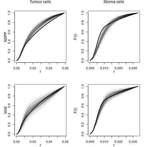
Figure 8: Figure showing for one patient’s slide (Figure 3) the fitted empty space function, F(r), by the solid line, and those for 100 simulated patterns (simulated using the estimated parameter values for each process), dotted lines.

References

- Beck (2011) {bbook}[author] \bauthor\bsnmBeck, \bfnmJudith S\binitsJ. S. (\byear2011). \btitleCognitive behavior therapy: Basics and beyond. \bpublisherGuilford Press. \endbibitem
- Caie and Harrison (2016) {barticle}[author] \bauthor\bsnmCaie, \bfnmPeter D\binitsP. D. and \bauthor\bsnmHarrison, \bfnmDavid J\binitsD. J. (\byear2016). \btitleNext-Generation Pathology. \bjournalSystems Medicine \bpages61–72. \endbibitem
- Caie et al. (2014) {barticle}[author] \bauthor\bsnmCaie, \bfnmPeter D\binitsP. D., \bauthor\bsnmTurnbull, \bfnmArran K\binitsA. K., \bauthor\bsnmFarrington, \bfnmSusan M\binitsS. M., \bauthor\bsnmOniscu, \bfnmAnca\binitsA. and \bauthor\bsnmHarrison, \bfnmDavid J\binitsD. J. (\byear2014). \btitleQuantification of tumour budding, lymphatic vessel density and invasion through image analysis in colorectal cancer. \bjournalJournal of Translational Medicine \bvolume12 \bpages1. \endbibitem
- Cannon, Cowen and Priebe (1998) {barticle}[author] \bauthor\bsnmCannon, \bfnmAdam H\binitsA. H., \bauthor\bsnmCowen, \bfnmLenore J\binitsL. J. and \bauthor\bsnmPriebe, \bfnmCarey E\binitsC. E. (\byear1998). \btitleApproximate distance classification. \bjournalComputing Science and Statistics \bpages544–549. \endbibitem
- De Smedt, Palmans and Sagaert (2016) {barticle}[author] \bauthor\bsnmDe Smedt, \bfnmLinde\binitsL., \bauthor\bsnmPalmans, \bfnmSofie\binitsS. and \bauthor\bsnmSagaert, \bfnmXavier\binitsX. (\byear2016). \btitleTumour budding in colorectal cancer: what do we know and what can we do? \bjournalVirchows Archiv \bvolume468 \bpages397–408. \endbibitem
- Definiens (2000) {bmisc}[author] \bauthor\bsnmDefiniens (\byear2000). \btitleDefiniens. \bhowpublishedhttp://www.definiens.com. \endbibitem
- DeVinney and Priebe (2006) {barticle}[author] \bauthor\bsnmDeVinney, \bfnmJason\binitsJ. and \bauthor\bsnmPriebe, \bfnmCarey E\binitsC. E. (\byear2006). \btitleA new family of proximity graphs: Class cover catch digraphs. \bjournalDiscrete Applied Mathematics \bvolume154 \bpages1975–1982. \endbibitem
- Diggle (2013) {bbook}[author] \bauthor\bsnmDiggle, \bfnmPeter J\binitsP. J. (\byear2013). \btitleStatistical analysis of spatial and spatio-temporal point patterns. \bpublisherCRC Press. \endbibitem
- Dubé et al. (2001) {barticle}[author] \bauthor\bsnmDubé, \bfnmP\binitsP., \bauthor\bsnmFortin, \bfnmMJ\binitsM., \bauthor\bsnmCanham, \bfnmCD\binitsC. and \bauthor\bsnmMarceau, \bfnmDJ\binitsD. (\byear2001). \btitleQuantifying gap dynamics at the patch mosaic level using a spatially-explicit model of a northern hardwood forest ecosystem. \bjournalEcological modelling \bvolume142 \bpages39–60. \endbibitem
- Gelfand et al. (2010) {bbook}[author] \bauthor\bsnmGelfand, \bfnmAlan E\binitsA. E., \bauthor\bsnmDiggle, \bfnmPeter\binitsP., \bauthor\bsnmGuttorp, \bfnmPeter\binitsP. and \bauthor\bsnmFuentes, \bfnmMontserrat\binitsM. (\byear2010). \btitleHandbook of spatial statistics. \bpublisherCRC Press. \endbibitem
- Heindl, Nawaz and Yuan (2015) {barticle}[author] \bauthor\bsnmHeindl, \bfnmAndreas\binitsA., \bauthor\bsnmNawaz, \bfnmSidra\binitsS. and \bauthor\bsnmYuan, \bfnmYinyin\binitsY. (\byear2015). \btitleMapping spatial heterogeneity in the tumor microenvironment: a new era for digital pathology. \bjournalLaboratory Investigation \bvolume95 \bpages377–384. \endbibitem
- Illian et al. (2008) {bbook}[author] \bauthor\bsnmIllian, \bfnmJanine\binitsJ., \bauthor\bsnmPenttinen, \bfnmAntti\binitsA., \bauthor\bsnmStoyan, \bfnmHelga\binitsH. and \bauthor\bsnmStoyan, \bfnmDietrich\binitsD. (\byear2008). \btitleStatistical analysis and modelling of spatial point patterns \bvolume70. \bpublisherJohn Wiley & Sons. \endbibitem
- Illian et al. (2013) {barticle}[author] \bauthor\bsnmIllian, \bfnmJanine B\binitsJ. B., \bauthor\bsnmMartino, \bfnmSara\binitsS., \bauthor\bsnmSørbye, \bfnmSigrunn H\binitsS. H., \bauthor\bsnmGallego-Fernández, \bfnmJuan B\binitsJ. B., \bauthor\bsnmZunzunegui, \bfnmMaria\binitsM., \bauthor\bsnmEsquivias, \bfnmM Paz\binitsM. P. and \bauthor\bsnmTravis, \bfnmJustin MJ\binitsJ. M. (\byear2013). \btitleFitting complex ecological point process models with integrated nested Laplace approximation. \bjournalMethods in Ecology and Evolution \bvolume4 \bpages305–315. \endbibitem
- Karamitopoulou et al. (2015) {barticle}[author] \bauthor\bsnmKaramitopoulou, \bfnmEva\binitsE., \bauthor\bsnmZlobec, \bfnmInti\binitsI., \bauthor\bsnmKoelzer, \bfnmViktor Hendrik\binitsV. H., \bauthor\bsnmLanger, \bfnmRupert\binitsR., \bauthor\bsnmDawson, \bfnmHeather\binitsH. and \bauthor\bsnmLugli, \bfnmAlessandro\binitsA. (\byear2015). \btitleTumour border configuration in colorectal cancer: proposal for an alternative scoring system based on the percentage of infiltrating margin. \bjournalHistopathology \bvolume67 \bpages464–473. \endbibitem
- Kauffmann and Fairall (1991) {barticle}[author] \bauthor\bsnmKauffmann, \bfnmG\binitsG. and \bauthor\bsnmFairall, \bfnmAP\binitsA. (\byear1991). \btitleVoids in the distribution of galaxies: an assessment of their significance and derivation of a void spectrum. \bjournalMonthly Notices of the Royal Astronomical Society \bvolume248 \bpages313–324. \endbibitem
- Li (2011) {barticle}[author] \bauthor\bsnmLi, \bfnmShengqiao\binitsS. (\byear2011). \btitleConcise formulas for the area and volume of a hyperspherical cap. \bjournalAsian Journal of Mathematics and Statistics \bvolume4 \bpages66–70. \endbibitem
- Marchette (2005) {bbook}[author] \bauthor\bsnmMarchette, \bfnmDavid J\binitsD. J. (\byear2005). \btitleRandom graphs for statistical pattern recognition \bvolume565. \bpublisherJohn Wiley & Sons. \endbibitem
- Matérn (2013) {bbook}[author] \bauthor\bsnmMatérn, \bfnmBertil\binitsB. (\byear2013). \btitleSpatial variation \bvolume36. \bpublisherSpringer Science & Business Media. \endbibitem