A Tube Dynamics Perspective Governing Stability Transitions: An Example Based on Snap-through Buckling

Abstract

The equilibrium configuration of an engineering structure, able to withstand a certain loading condition, is usually associated with a local minimum of the underlying potential energy. However, in the nonlinear context, there may be other equilibria present, and this brings with it the possibility of a transition to an alternative (remote) minimum. That is, given a sufficient disturbance, the structure might buckle, perhaps suddenly, to another shape. This paper considers the dynamic mechanisms under which such transitions (typically via saddle points) occur. A two-mode Hamiltonian is developed for a shallow arch/buckled beam. The resulting form of the potential energy—two stable wells connected by rank-1 saddle points—shows an analogy with resonance transitions in celestial mechanics or molecular reconfigurations in chemistry, whereas here the transition corresponds to switching between two stable structural configurations. Then, from Hamilton’s equations, the analytical equilibria are determined and linearization of the equations of motion about the saddle is obtained. After computing the eigenvalues and eigenvectors of the coefficient matrix associated with the linearization, a symplectic transformation is given which puts the Hamiltonian into normal form and simplifies the equations, allowing us to use the conceptual framework known as tube dynamics. The flow in the equilibrium region of phase space as well as the invariant manifold tubes in position space are discussed. Also, we account for the addition of damping in the tube dynamics framework, which leads to a richer set of behaviors in transition dynamics than previously explored.

1 Introduction

The nonlinear behavior of slender structures under loading is often dominated by a potential energy function that possesses a number of stationary points corresponding to various equilibrium configurations [1, 2]. Some are stable (local minima, or ‘well’), some are unstable (local maxima or ‘hill-top’), and some correspond to saddle points, i.e., a shape with opposite curvature in different directions, but still unstable, having both stable and unstable directions. Interestingly, although difficult to observe experimentally, it is these saddle points that can have a profound organizing effect on global trajectories in a dynamics context. Thus, under a nominally fixed set of loads or a given configuration we may have the situation in which a system is at rest in a position of stable equilibrium, but, given sufficiently large perturbation (input of energy) may transition to a remote stable equilibrium [3], or even collapse completely [4, 5]. The path taken during this transition is associated with the least energetic route, and this will typically correspond to a passage close to a saddle point: it is easier to take a path around a mountain than going directly over its peak.

For a single mechanical degree of freedom the transition from one potential energy minimum to another is relatively unambiguous [6, 7]. We can think of a twin-well oscillator and how it has no choice but to pass over an intermediate hilltop in transitioning to an adjacent minimum. For high-order systems trajectories have many more possible paths. But a system with two mechanical degrees of freedom (configuration space), and thus a 4 dimensional phase space, offers an intermediate situation: compelling conceptual clarity (i.e., the potential energy can be thought of as a surface or landscape), but still retaining a wider range of potential behavior over and above the aforementioned single oscillator (i.e., multiple ways of traversing and perhaps escaping from one potential well to another).

For the two degree of freedom system, the analog of the hilltop is the saddle point of the potential energy surface. The linearized dynamics near such a point yield an oscillatory mode and an exponential mode, with both asymptotically stable and unstable directions. For energies slightly above the saddle point, there is a bottleneck to the energy surface [8, 9]. Transitions from one side of the bottleneck can be understood in terms of sets of trajectories which are bounded by topological cylinders. The transition dynamics, which has in some contexts been known as tube dynamics [10, 11, 12, 13, 14, 15, 9, 16, 17, 18, 19], has been developed for studying transitions between stable states (the potential wells) in a number of disparate contexts, and here it is applied to a structural mechanics situation in which snap-through buckling [2] is the key phenomenological transition. Conditions are determined whereby the initial energy imparted to the system is characterized in terms of subsequent escape from the initial potential well.

2 The Paradigm: Snap-through of an Arch/Buckled Beam

A classic example of a saddle-node bifurcation in structural mechanics is the symmetric snap-through buckling of a shallow arch, in an essentially co-dimension 1 bifurcation [7]. However, if the arch (or equivalently a buckled beam) is not shallow then the typical mechanism of instability is an asymmetric snap-through, requiring two modes (symmetric and asymmetric) for characterization, and the instability corresponds to a subcritical pitchfork bifurcation. In both of these cases the transition is sudden and associated with a fast dynamic jump, since there is no longer any locally available stable equilibrium. This behavior is generic regardless of boundary conditions and is also exhibited by the laterally-loaded buckled beam [20, 21]. We shall focus on this latter example, for relative simplicity of introduction. The essential focus here is that the underlying potential energy of this system consists of two potential energy wells (the original unloaded equilibrium and the snapped-through equilibrium), an unstable hilltop (the intermediate, straight, unstable equilibrium) and two saddle-points. The symmetry of this system is broken by small geometric imperfections. The question is: how does the system escape its local potential energy well in a dynamical systems sense?

Suppose we have a moderately buckled beam. If a central point load is applied then the beam deflects initially in a purely symmetric mode, as shown by the red line in Fig. 1(a), following the $\alpha$ loading path.

Figure 1: (a) A schematic load-deflection characteristic, (b) the two dominant degrees of freedom.

Upon a quasi-static increase in the load $P$, point $C$ is reached (a subcritical pitchfork bifurcation) and the arch quickly snaps-through (a thoroughly dynamic event) with a significant asymmetric component in the deflection and the system settles into its inverted position $D$ [3]. This behavior is captured by considering a two-mode analysis: sag $S$ (symmetric) and angle $A$ (asymmetric), or alternatively we can use the harmonic coordinates $X$ and $Y$, respectively, corresponding to the modes in part (b). In an approximate analysis they might be the lowest two buckling modes or free vibration modes from a standard eigen-analysis. Suppose we load the beam to a value slightly below the snap value at $P_{C}$, and fix it at that value. In this case there will be the five equilibria mentioned earlier: three equilibria purely in sag (two stable and an unstable one between them), and two saddles, with significant angular components but geometrically opposed [1]. Small geometric imperfections (in $A$ and/or $S$) will break the symmetry and influence which path is more likely to be followed. In this fixed configuration we can then think of the system in dynamic terms, and consider the range of initial conditions (including velocity, perhaps caused by an impact force) that might push the system from a point on path $\alpha$ to a point on path $\phi$.

Governing equations

In this analysis a slender buckled beam with thickness $d$, width $b$ and length $L$ is considered. A Cartesian coordinate system $o\textendash xyz$ is established on the mid-plane of the beam in which $o$ is the origin, $x,y$ the directions along the length and width directions and $z$ the downward direction normal to the mid-plane. Based on Euler-Bernoulli beam theory [22, 1], the displacement field $(u_{1},u_{3})$ of the beam along $(x,z)$ directions can be written as

$$\begin{split}u_{1}(x,z,t)&=u(x,t)-z\frac{\partial w(x,t)}{\partial x}\\ u_{3}(x,z,t)&=w(x,t)\end{split}$$ (1)

where $u(x,t)$ and $w(x,t)$ are the axial and transverse displacements of an arbitrary point on the mid-plane of the beam. Considering the von Kámán-type geometrical nonlinearity, the total axial strain can be obtained as

$$\begin{split}\varepsilon^{*}_{x}=\frac{\partial u}{\partial x}-z\frac{\partial^{2}w}{\partial x^{2}}+\frac{1}{2}\left(\frac{\partial w}{\partial x}\right)^{2}\end{split}$$ (2)

For a moderately buckled-beam, we need to consider the initial strain $\varepsilon_{0}$ produced by initial deflection $w_{0}$ which is

$$\begin{split}\varepsilon_{0}=-z\frac{\partial^{2}w_{0}}{\partial x^{2}}+\frac{1}{2}\left(\frac{\partial w_{0}}{\partial x}\right)^{2}\end{split}$$ (3)

Then the change in strain $\varepsilon_{x}$ can be expressed as

$$\begin{split}\varepsilon_{x}=\varepsilon^{*}_{x}-\varepsilon_{0}=\frac{\partial u}{\partial x}-z\left(\frac{\partial^{2}w}{\partial x^{2}}-\frac{\partial^{2}w_{0}}{\partial x^{2}}\right)+\frac{1}{2}\left[\left(\frac{\partial w}{\partial x}\right)^{2}-\left(\frac{\partial w_{0}}{\partial x}\right)^{2}\right]\end{split}$$ (4)

Here we just consider homogeneous isotropic materials with Young’s modulus $E$, and allow for the possibility of thermal loading. The axial stress $\sigma_{x}$ can be obtained according to the one dimensional constitutive equation, as

$$\begin{split}\sigma_{x}=E\varepsilon_{x}-E\alpha_{x}\Delta T\end{split}$$ (5)

where $\alpha_{x}$ is the thermal expansion coefficient and $\Delta T$ is the temperature increment from the reference temperature at which the beam is in a stress free state. Thermal loading is introduced as a convenient way of controlling the initial equilibrium shapes (and hence the potential energy landscape) via axial loading.

The strain energy $\mathcal{V}(x,z,t)$ is

$$\begin{split}\mathcal{V}(x,z,t)&=\frac{b}{2}\int_{0}^{L}\int_{-\frac{d}{2}}^{\frac{d}{2}}\sigma_{x}\varepsilon_{x}\mathrm{d}z\mathrm{d}x\end{split}$$ (6)

Ignoring the axial inertia term, the kinetic energy $\mathcal{T}(x,z,t)$ of the buckled beam is

$$\begin{split}\mathcal{T}(x,z,t)=\frac{b}{2}\int_{0}^{L}\int_{-\frac{d}{2}}^{\frac{d}{2}}\rho\dot{w}^{2}\mathrm{d}z\mathrm{d}x\end{split}$$ (7)

where $\rho$ is the mass density. In addition, the dot over the quantity is the derivative with respective to time.

The governing equations can be obtained by Hamilton’s principle which requires that

$$\begin{split}\delta\int_{t_{0}}^{t}\left[\mathcal{T}(x,z,t)-\mathcal{V}(x,z,t)\right]\mathrm{d}t+\int_{t_{0}}^{t}\delta W_{nc}\mathrm{d}t=0\end{split}$$ (8)

where $\delta$ denotes the variational operator, $t_{0}$ and $t$ the initial and current time. $\delta W_{nc}$ is the variation of the virtual work done by non-conservative force (damping) which is expressed as

$$\begin{split}\delta W_{nc}=-c_{d}\dot{w}\delta w\end{split}$$ (9)

where $c_{d}$ is the coefficient of (linear viscous) damping. In subsequent analysis, and related to typical practical situations, the damping will be small.

After some manipulation, the governing equations in terms of axial force $N_{x}$ and bending moment $M_{x}$ can be obtained as [22]

$$\begin{split}&\frac{\partial N_{x}}{\partial x}=0\\ &\frac{\partial^{2}M_{x}}{\partial x^{2}}+N_{x}\frac{\partial^{2}w}{\partial x^{2}}=\rho A\ddot{w}+c_{d}\dot{w}\end{split}$$ (10)

where $N_{x}$ and $M_{x}$ are defined as

$$\begin{split}\left(N_{x},M_{x}\right)=b\int_{-\frac{d}{2}}^{\frac{d}{2}}\end{split}\sigma_{x}\left(1,z\right)\mathrm{d}z$$ (11)

By using (1), (4) and (5), the force $N_{x}$ and moment $M_{x}$ in (11) can be rewritten as

$$\begin{split}N_{x}&=EA\left[\frac{\partial u}{\partial x}+\frac{1}{2}\left(\left(\frac{\partial w}{\partial x}\right)^{2}-\left(\frac{\partial w_{0}}{\partial x}\right)^{2}\right)\right]-N_{T}\\ M_{x}&=-EI\left(\frac{\partial^{2}w}{\partial x^{2}}-\frac{\partial^{2}w_{0}}{\partial x^{2}}\right)\end{split}$$ (12)

where $A$ and $I$ denote the cross-sectional area and moment of inertia; $N_{T}=EA\alpha_{x}\Delta T$, the axial thermal loads. Thus, $EA$ and $EI$ are the axial stiffness and bending stiffness, respectively.

Here we just consider a clamped-clamped beam with in-plane immovable ends. The boundary conditions are

$$\begin{split}x=0,L:u=w=\frac{\partial w}{\partial x}=0\end{split}$$ (13)

Note that from the first equation in (10), it is clear that the axial force $N_{x}$ is constant along the axial direction. In this case, integrating the axial force along the $x$ axis and using the boundary conditions $u(0,t)=u(L,t)=0$, one can obtain

$$\begin{split}N_{x}=\frac{EA}{2L}\int_{0}^{L}\left[\left(\frac{\partial w}{\partial x}\right)^{2}-\left(\frac{\partial w_{0}}{\partial x}\right)^{2}\right]\mathrm{d}x-N_{T}\end{split}$$ (14)

Using $M_{x}$ in (12) and $N_{x}$ in (14), the second equation in (10) can be described in terms of the transverse displacement $w$ as [1]

$$\begin{split}\rho A\ddot{w}+c_{d}\dot{w}+EI\left(\frac{\partial^{4}w}{\partial x^{4}}-\frac{\partial^{4}w_{0}}{\partial x^{4}}\right)+\left[N_{T}-\frac{EA}{2L}\int_{0}^{L}\left(\left(\frac{\partial w}{\partial x}\right)^{2}-\left(\frac{\partial w_{0}}{\partial x}\right)^{2}\right)\mathrm{d}x\right]\frac{\partial^{2}w}{\partial x^{2}}=0\end{split}$$ (15)

where $w$ and $w_{0}$ are the current deflection and initial geometrical imperfection, respectively; $\rho$ is the mass density; $c_{d}$ is the damping coefficient; $A$ and $I$ are the area and the moment of inertia of the cross-section, respectively; $E$ is the Young’s modulus. Given the immovable ends it is natural to consider the effective externally applied axial force to be replaced by a thermal loading term: this is the primary destabilizing nonlinearity in the system.

As mentioned earlier, clamped-clamped boundary conditions are considered. Thus we make use of the mode shapes

$$\begin{split}&\phi_{n}=\alpha_{n}\left[\sinh\frac{\beta_{n}x}{L}-\sin\frac{\beta_{n}x}{L}+\delta_{n}\left(\cosh\frac{\beta_{n}x}{L}-\cos\frac{\beta_{n}x}{L}\right)\right],\\ &\delta_{n}=\frac{\sinh\beta_{n}-\sin\beta_{n}}{\cos\beta_{n}-\cosh\beta_{n}},\\ &\cos\beta_{n}\cosh\beta_{n}=1,\\ &\alpha_{1}=-0.6186,\ \ \ \alpha_{2}=-0.6631\end{split}$$ (16)

and describe the deflected shape in terms of a two-degree-of-freedom approximation

$$\begin{split}w(x,t)&=X(t)\phi_{1}(x)+Y(t)\phi_{2}(x),\\ w_{0}(x)&=\gamma_{1}\phi_{1}(x)+\gamma_{2}\phi_{2}(x)\end{split}$$ (17)

where the initial imperfections are given by $w_{0}$. Substituting the assumed solution into the equation of motion  15 yields

$$\begin{split}&\rho A\int_{0}^{L}\phi_{i}\ddot{w}\mathrm{d}x+c_{d}\int_{0}^{L}\phi_{i}\dot{w}\mathrm{d}x+EI\int_{0}^{L}\frac{\partial^{2}\phi_{i}}{\partial x^{2}}\left(\frac{\partial^{2}w}{\partial x^{2}}-\frac{\partial^{2}w_{0}}{\partial x^{2}}\right)\mathrm{d}x\\ &-\left[N_{T}-\frac{EA}{2L}\int_{0}^{L}\left(\left(\frac{\partial w}{\partial x}\right)^{2}-\left(\frac{\partial w_{0}}{\partial x}\right)^{2}\right)\mathrm{d}x\right]\int_{0}^{L}\frac{\partial\phi_{i}}{\partial x}\frac{\partial w}{\partial x}\mathrm{d}x=0\end{split}$$ (18)

Using the specific forms of $\phi_{i}$ in (16) and noticing each mode shape is orthogonal, the nonlinear equations can be obtained

$$\begin{split}&M_{1}\ddot{X}+C_{1}\dot{X}+K_{1}\left(X-\gamma_{1}\right)-N_{T}G_{1}X-\frac{EA}{2L}G_{1}^{2}\left(\gamma_{1}^{2}X-X^{3}\right)-\frac{EA}{2L}G_{1}G_{2}\left(\gamma_{2}^{2}X-XY^{2}\right)=0\\ &M_{2}\ddot{Y}+C_{2}\dot{Y}+K_{2}\left(Y-\gamma_{2}\right)-N_{T}G_{2}Y-\frac{EA}{2L}G_{2}^{2}\left(\gamma_{2}^{2}Y-Y^{3}\right)-\frac{EA}{2L}G_{1}G_{2}\left(\gamma_{1}^{2}Y-X^{2}Y\right)=0\end{split}$$ (19)

where

$$\begin{split}\left(M_{i},C_{i}\right)=\left(\rho A,c_{d}\right)\int_{0}^{L}\phi_{i}^{2}\mathrm{d}x,\ \ K_{i}=EI\int_{0}^{L}\left(\frac{\partial^{2}\phi_{i}}{\partial x^{2}}\right)^{2}\mathrm{d}x,\ \ G_{i}=\int_{0}^{L}\left(\frac{\partial\phi_{i}}{\partial x}\right)^{2}\mathrm{d}x\end{split}$$ (20)

The kinetic energy and potential energy, respectively, can be represented as

$$\begin{split}\mathcal{T}(\dot{X},\dot{Y})=&\frac{1}{2}M_{1}\dot{X}^{2}+\frac{1}{2}M_{2}\dot{Y}^{2},\\ \mathcal{V}(X,Y)=&-K_{1}\gamma_{1}X-K_{2}\gamma_{2}Y+\frac{1}{2}K_{1}X^{2}+\frac{1}{2}K_{2}Y^{2}-\frac{1}{2}N_{T}\left(G_{1}X^{2}+G_{2}Y^{2}\right)\\ &-\frac{EA}{2L}G_{1}^{2}\left(\frac{1}{2}\gamma_{1}^{2}X^{2}-\frac{1}{4}X^{4}\right)-\frac{EA}{2L}G_{2}^{2}\left(\frac{1}{2}\gamma_{2}^{2}Y^{2}-\frac{1}{4}Y^{4}\right)\\ &-\frac{EA}{2L}\frac{G_{1}G_{2}}{2}\left(\gamma_{2}^{2}X^{2}+\gamma_{1}^{2}Y^{2}-X^{2}Y^{2}\right).\\ \end{split}$$ (21)

For physically reasonable coefficients we have a number of equilibrium possibilities. For small values of $N_{T}$ we have an essentially linear system, dominated by the trivial (straight) equilibrium configuration, and thus an isolated center (minimum of the potential energy). This relates back to the situation in Figure 1 for a small value of $P$. But for larger values of $P$, for example a little below $P_{c}$, the system typically possesses a number of equilibria, some of which are stable and some of which are not. Some typical forms are shown in Figure 2(a) in which the five dots are the equilibrium points where W₁ and W₂ are within the two stable wells; S₁ and S₂ two unstable saddle points; H the unstable hilltop. Thus, we might have the system sitting (in equilibrium) at point W₁. If it is then subject to a disturbance with the right size and direction (in the dynamical context), we might expect the system to transition to the remote equilibrium at W₂. This might occur when the system is subject to a large impact force, for example [21]. It is anticipated (and will later be shown) that the typically easiest transition will be associated with (an asymmetric) passage close to S₁ or S₂, and generally avoiding H. In Figure 2(b) is shown the same system but now with a small geometric imperfection in both modes (i.e., $\gamma_{1}\neq 0$ and $\gamma_{2}\neq 0$). In this case the symmetry of the system is broken, and given the relative energy associated with the saddle points it is anticipated (and will also be shown later) that optimal escape will tend to occur via S₁.

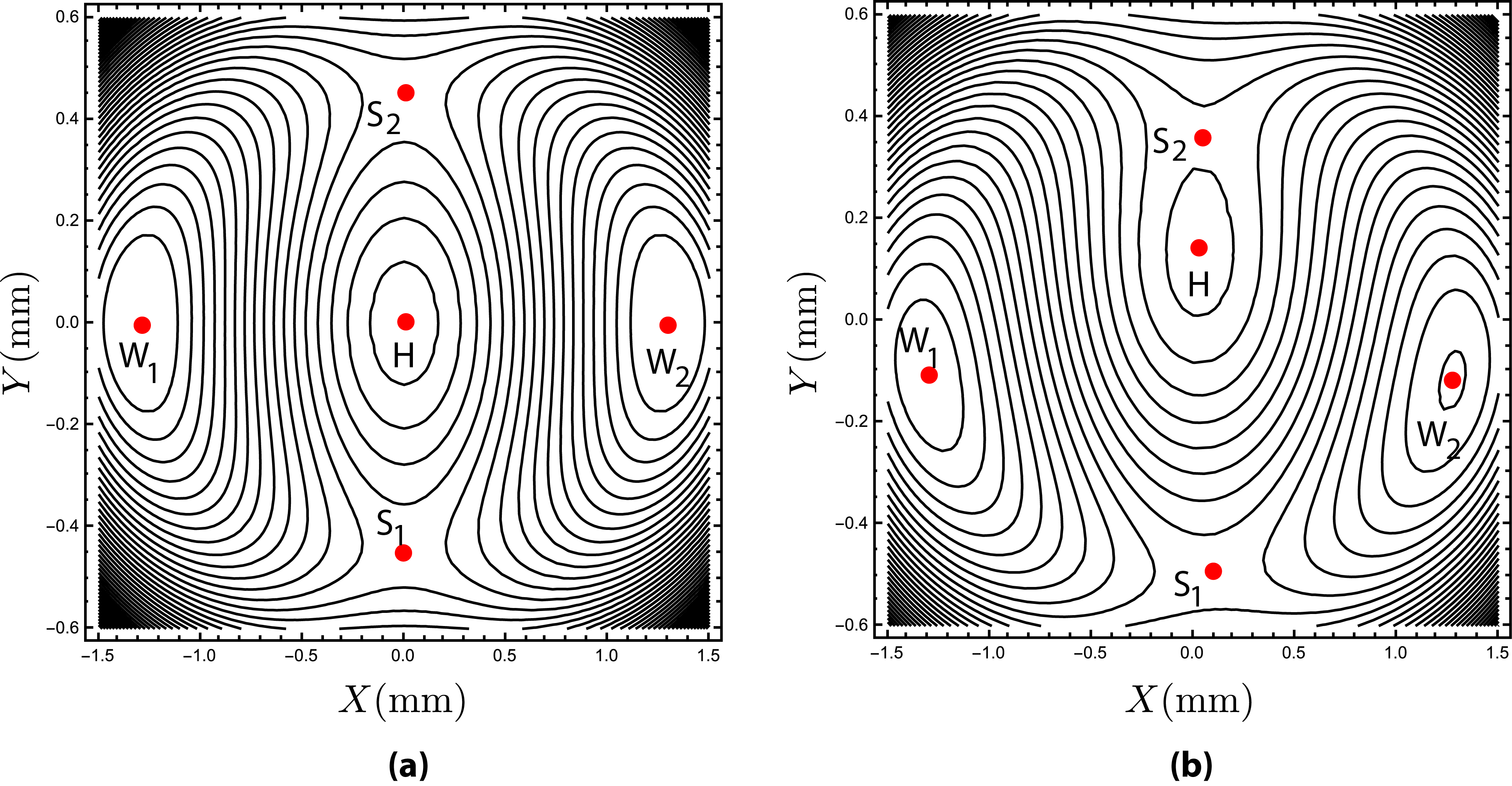
Figure 2: Contours of potential energy: (a) the symmetric system, $\gamma_{1}=\gamma_{2}=0$, (b) with small initial imperfections in both modes, i.e., $\gamma_{1}$ and $\gamma_{2}$ are nonzero.

Note that eqs. (19) can also be obtained from Lagrange’s equations,

$$\frac{d}{dt}\left(\frac{\partial\mathcal{L}}{\partial\dot{q}_{i}}\right)-\frac{\partial\mathcal{L}}{\partial q_{i}}=-C_{i}\dot{q}_{i},\quad i=1,2$$ (22)

when $q_{1}=X$ and $q_{2}=Y$, and the Lagrangian is

$$\mathcal{L}(X,Y,\dot{X},\dot{Y})=\mathcal{T}(\dot{X},\dot{Y})-\mathcal{V}(X,Y)$$ (23)

To transform this to a Hamiltonian system, one defines the generalized momenta,

$$\begin{split}p_{i}=\frac{\partial\mathcal{L}}{\partial\dot{q}_{i}}=M_{i}\dot{q}_{i}\end{split}$$ (24)

so $p_{X}=M_{1}\dot{X}$ and $p_{Y}=M_{2}\dot{Y}$, in which case, the kinetic energy is

$$\mathcal{T}(X,Y,p_{X},p_{Y})=\frac{1}{2M_{1}}p_{X}^{2}+\frac{1}{2M_{2}}p_{Y}^{2}$$ (25)

and the Hamiltonian is

$$\mathcal{H}(X,Y,p_{X},p_{Y})=\mathcal{T}+\mathcal{V}$$ (26)

and Hamilton’s equations (with damping) [23] are

$$\begin{split}\dot{X}&=\frac{\partial\mathcal{H}}{\partial p_{X}}=\frac{p_{X}}{M_{1}}\\ \dot{Y}&=\frac{\partial\mathcal{H}}{\partial p_{Y}}=\frac{p_{y}}{M_{2}}\\ \dot{p}_{X}&=-\frac{\partial\mathcal{H}}{\partial X}-C_{H}p_{X}=-\frac{\partial\mathcal{V}}{\partial X}-C_{H}p_{X}\\ \dot{p}_{Y}&=-\frac{\partial\mathcal{H}}{\partial Y}-C_{H}p_{Y}=-\frac{\partial\mathcal{V}}{\partial Y}-C_{H}p_{Y}\\ \end{split}$$ (27)

where

$$\begin{split}\frac{\partial\mathcal{V}}{\partial X}=&K_{1}\left(X-\gamma_{1}\right)-N_{T}G_{1}X-\frac{EA}{2L}G_{1}^{2}\left(\gamma_{1}^{2}X-X^{3}\right)-\frac{EA}{2L}G_{1}G_{2}\left(\gamma_{2}^{2}X-XY^{2}\right),\\ \frac{\partial\mathcal{V}}{\partial Y}=&K_{2}\left(Y-\gamma_{2}\right)-N_{T}G_{2}Y-\frac{EA}{2L}G_{2}^{2}\left(\gamma_{2}^{2}Y-Y^{3}\right)-\frac{EA}{2L}G_{1}G_{2}\left(\gamma_{1}^{2}Y-X^{2}Y\right)\end{split}$$ (28)

and $C_{H}=C_{1}/M_{1}=C_{2}/M_{2}$ is the damping coefficient in the Hamiltonian system which can be easily found by comparing (19) and (LABEL:eq:eomHam), and using the relations of $M_{i}$ and $C_{i}$ in (20).

We assume the lower saddle point S₁ has the smaller potential energy compared to S₂, thus the energy of S₁ is the critical energy for snap-though, and we initially focus attention on the dynamic behavior around the region of S₁. The linearized equations of (LABEL:eq:eomHam) about S₁ with position $(X_{e},Y_{e})$ can be written as

$$\begin{split}\dot{x}&=\frac{p_{x}}{M_{1}}\\ \dot{y}&=\frac{p_{y}}{M_{2}}\\ \dot{p}_{x}&=A_{31}x+A_{32}y-C_{H}p_{x}\\ \dot{p}_{y}&=A_{32}x+A_{42}y-C_{H}p_{y}\end{split}$$ (29)

where $(x,y,p_{x},p_{y})=(X,Y,p_{X},p_{Y})-(X_{e},Y_{e},0,0)$ and

$$\begin{split}&A_{31}=-K_{1}+N_{T}G_{1}+\frac{EAG_{1}^{2}\left(\gamma_{1}^{2}-3X_{e}^{2}\right)}{2L}+\frac{EAG_{1}G_{2}\left(\gamma_{2}^{2}-Y_{e}^{2}\right)}{2L},\\ &A_{32}=-\frac{EAG_{1}G_{2}X_{e}Y_{e}}{L},\\ &A_{42}=-K_{2}+N_{T}G_{2}+\frac{EAG_{2}^{2}\left(\gamma_{2}^{2}-3Y_{e}^{2}\right)}{2L}+\frac{EAG_{1}G_{2}\left(\gamma_{1}^{2}-X_{e}^{2}\right)}{2L}\end{split}$$ (30)

If we replace the position of S₁ by the position of W₁, we can still use the linearized equations in (29) to obtain the natural frequencies of the shallow arch near W₁ as

$$\omega_{1,2}^{(d)}=w_{1,2}^{(c)}\sqrt{1-\xi_{1,2}^{2}}$$ (31)

where $\omega_{1,2}^{(c)}$ are the first two natural frequencies for the conservative system and $\xi_{1,2}$ are the viscous damping factors with the forms

$$\omega_{1,2}^{(c)}=\frac{(b_{\omega}\mp\sqrt{b_{\omega}^{2}-4c_{\omega}})}{2},\hskip 36.135pt\xi_{1,2}=\frac{C_{H}}{2\omega_{1,2}^{(c)}}$$ (32)

and

$$b_{\omega}=-\frac{A_{31}}{M_{1}}-\frac{A_{42}}{M_{2}},\hskip 36.135ptc_{\omega}=\frac{A_{31}A_{42}-A_{32}^{2}}{M_{1}M_{2}}$$

Non-dimensional equations of motion

In order to reduce the parameters, some non-dimensional quantities are introduced,

$$\begin{split}&\left(L_{x},L_{y}\right)=L\left(1,\sqrt{\frac{M_{1}}{M_{2}}}\right),\omega_{0}=\frac{\sqrt{-A_{32}}}{\left(M_{1}M_{2}\right)^{\frac{1}{4}}},\tau=\omega_{0}t,\left(\bar{q}_{1},\bar{q}_{2}\right)=\left(\frac{x}{L_{x}},\frac{y}{L_{y}}\right),\\ &\left(\bar{p}_{1},\bar{p}_{2}\right)=\frac{1}{\omega_{0}}\left(\frac{p_{x}}{L_{x}M_{1}},\frac{p_{y}}{L_{y}M_{2}}\right),\left(c_{x},c_{y}\right)=\frac{1}{\omega_{0}^{2}}\left(\frac{A_{31}}{M_{1}},\frac{A_{42}}{M_{2}}\right),c_{1}=\frac{C_{H}}{\omega_{0}}\end{split}$$ (33)

Using the non-dimensional parameters in (33), the non-dimensional linearized equations are written as

$$\begin{split}\dot{\bar{q}}_{1}&=\bar{p}_{1},\\ \dot{\bar{q}}_{2}&=\bar{p}_{2},\\ \dot{\bar{p}}_{1}&=c_{x}\bar{q}_{1}-\bar{q}_{2}-c_{1}\bar{p}_{1},\\ \dot{\bar{p}}_{2}&=-\bar{q}_{1}+c_{y}\bar{q}_{2}-c_{1}\bar{p}_{2}\end{split}$$ (34)

Written in matrix form, with column vector $\bar{z}=(\bar{q}_{1},\bar{q}_{2},\bar{p}_{1},\bar{p}_{2})$, we have

$$\dot{\bar{z}}=A\bar{z}+D\bar{z}$$

where

$$A=\begin{pmatrix}0&0&1&0\\ 0&0&0&1\\ c_{x}&-1&0&0\\ -1&c_{y}&0&0\end{pmatrix},\hskip 36.135ptD=\begin{pmatrix}0&0&0&0\\ 0&0&0&0\\ 0&0&-c_{1}&0\\ 0&0&0&-c_{1}\end{pmatrix}$$ (35)

are the Hamiltonian part and damping part of the linear equations, respectively.

3 Linearized Conservative Hamiltonian System

3.1 Solutions near the equilibria

Eigenvalues and eigenvectors

In this section, we will discuss the linear dynamical behaviors of a buckled beam in the Hamiltonian system without taking account of any energy dissipation which makes $c_{1}=0$ (i.e., $C_{H}=0$). Thus, the equations of motion are given as

$$\dot{\bar{z}}=A\bar{z}$$ (36)

The system (36) can be viewed as resulting from a quadratic Hamiltonian,

$$\mathcal{H}_{2}=\tfrac{1}{2}\bar{p}_{1}^{2}+\tfrac{1}{2}\bar{p}_{2}^{2}-\tfrac{1}{2}c_{x}\bar{q}_{1}^{2}-\tfrac{1}{2}c_{y}\bar{q}_{2}^{2}+\bar{q}_{1}\bar{q}_{2}$$ (37)

which can be written in matrix form

$$\mathcal{H}_{2}=\frac{1}{2}\bar{z}^{T}B\bar{z}$$

where

$$\begin{split}B=J^{T}A=\begin{pmatrix}-c_{x}&1&0&0\\ 1&-c_{y}&0&0\\ 0&0&1&0\\ 0&0&0&1\end{pmatrix}\end{split}$$

and ${J}$ is the $4\times 4$ canonical symplectic matrix

$$\begin{split}{J}=\begin{pmatrix}{\bf 0}&{I}_{2}\\ -{I}_{2}&{\bf 0}\\ \end{pmatrix}\end{split}$$

where ${I}_{2}$ is the $2\times 2$ identity matrix.

The characteristic polynomial of (36) is

$$p(\beta)=\beta^{4}-(c_{x}+c_{y})\beta^{2}+c_{x}c_{y}-1$$

Let $\alpha=\beta^{2}$, then the roots of $p(\alpha)=0$ are as follows

$$\begin{split}\alpha_{1}=\frac{c_{x}+c_{y}+\sqrt{\left(c_{x}-c_{y}\right)^{2}+4}}{2},\\ \alpha_{2}=\frac{c_{x}+c_{y}-\sqrt{\left(c_{x}-c_{y}\right)^{2}+4}}{2}\end{split}$$ (38)

Generally, in (36) $c_{x}>0$ and $c_{y}<0$. In this case, $\alpha_{1}>0$ and $\alpha_{2}<0$. It follows that this equilibrium point is of the type saddle $\times$ center. Here we define $\lambda=\sqrt{\alpha_{1}}$ and $\omega_{p}=\sqrt{-\alpha_{2}}$. Thus, the eigenvectors are given by

$$\begin{split}\left(1,c_{x}-\beta^{2},\beta,c_{x}\beta-\beta^{3}\right),\end{split}$$ (39)

where $\beta$ denotes one of the eigenvalues.

After substituting $\beta=i\omega_{p}$ into (39) and separating real and imaginary parts as $u_{\omega_{p}}+iv_{\omega_{p}}$, we obtain two corresponding eigenvectors

$$\begin{split}u_{\omega_{p}}&=\left(1,c_{x}+\omega_{p}^{2},0,0\right),\\ v_{\omega_{p}}&=\left(0,0,\omega_{p},c_{x}\omega_{p}+\omega_{p}^{3}\right),\end{split}$$ (40)

Moreover, the other two eigenvectors associated with the pair of real eigenvalues $\pm\lambda$ can be taken as

$$\begin{split}u_{+\lambda}&=\left(1,c_{x}-\lambda^{2},\lambda,c_{x}\lambda-\lambda^{3}\right),\\ u_{-\lambda}&=-\left(1,c_{x}-\lambda^{2},-\lambda,\lambda^{3}-c_{x}\lambda\right)\end{split}$$ (41)

Symplectic change of variables

We consider the linear symplectic change of variables from $(\bar{q}_{1},\bar{q}_{2},\bar{p}_{1},\bar{p}_{2})$ to $(q_{1},q_{2},p_{1},p_{2})$,

$$\left(\begin{array}[]{c c c c}\bar{q}_{1}\\ \bar{q}_{2}\\ \bar{p}_{1}\\ \bar{p}_{2}\end{array}\right)=C\left(\begin{array}[]{c c c c}q_{1}\\ q_{2}\\ p_{1}\\ p_{2}\end{array}\right)$$ (42)

where the columns of the matrix $C$ are given by the eigenvectors,

$$\begin{split}C=\left(u_{+\lambda},u_{\omega_{p}},u_{-\lambda},v_{\omega_{p}}\right)\end{split}$$ (43)

and where the vectors are written as column vectors.

Then we find

$$\begin{split}C^{T}JC=\begin{pmatrix}0&\bar{D}\\ -\bar{D}&0\end{pmatrix},\hskip 36.135pt\bar{D}=\begin{pmatrix}d_{\lambda}&0\\ 0&d_{\omega_{p}}\end{pmatrix}\end{split}$$ (44)

where

$$\begin{split}d_{\lambda}&=\lambda[4-2(c_{x}-c_{y})(\lambda^{2}-c_{x})]\\ d_{\omega_{p}}&=\frac{\omega_{p}}{2}[4+2(c_{x}-c_{y})(\omega_{p}^{2}+c_{x})]\end{split}$$ (45)

In order to obtain a symplectic form which satisfies $C^{T}JC=J$, we need to rescale the columns of $C$. The scaling is given by factors $s_{1}=\sqrt{d_{\lambda}}$ and $s_{2}=\sqrt{d_{\omega_{p}}}$. In this case, the final form of the symplectic matrix $C$ is given by

$$\begin{split}C=\begin{pmatrix}\frac{1}{s_{1}}&\frac{1}{s_{2}}&-\frac{1}{s_{1}}&0\\ \frac{c_{x}-\lambda^{2}}{s_{1}}&\frac{\omega_{p}^{2}+c_{x}}{s_{2}}&\frac{\lambda^{2}-c_{x}}{s_{1}}&0\\ \frac{\lambda}{s_{1}}&0&\frac{\lambda}{s_{1}}&\frac{\omega_{p}}{s_{2}}\\ \frac{c_{x}\lambda-\lambda^{3}}{s_{1}}&0&\frac{c_{x}\lambda-\lambda^{3}}{s_{1}}&\frac{c_{x}\omega_{p}+\omega_{p}^{3}}{s_{2}}\end{pmatrix}\end{split}$$ (46)

The Hamiltonian (37) can be rewritten in the simplified, normal form,

$$\mathcal{H}_{2}=\lambda q_{1}p_{1}+\tfrac{1}{2}\omega_{p}(q_{2}^{2}+p_{2}^{2})$$ (47)

with corresponding linearized equations,

$$\begin{split}\dot{q}_{1}&=~{}~{}\lambda q_{1},\\ \dot{p}_{1}&=-\lambda p_{1},\\ \dot{q}_{2}&=~{}~{}\omega_{p}p_{2},\\ \dot{p}_{2}&=-\omega_{p}q_{2}\end{split}$$ (48)

Written in matrix form, with column vector $z=(q_{1},q_{2},p_{1},p_{2})$, we have

$$\dot{z}=\Lambda z$$

where

$$\begin{split}\Lambda=C^{-1}AC=\left(\begin{array}[]{rrrr}\lambda&0&0&0\\ 0&0&0&\omega_{p}\\ 0&0&-\lambda&0\\ 0&-\omega_{p}&0&0\end{array}\right)\end{split}$$ (49)

The solution of (48) can be written as

$$\begin{split}&q_{1}=q_{1}^{0}e^{\lambda t},\ \ \ p_{1}=p_{1}^{0}e^{-\lambda t}\\ &q_{2}+ip_{2}=\left(q_{2}^{0}+ip_{2}^{0}\right)e^{-i\omega_{p}t}\end{split}$$ (50)

Note that the three functions

$$f_{1}=q_{1}p_{1},\quad f_{2}=q_{2}^{2}+p_{2}^{2},\quad f_{3}=\mathcal{H}_{2}$$

are constants of motion under the Hamiltonian system (48).

3.2 Boundary of transit and non-transit orbits

The Linearized Phase Space

For positive $h$ and $c$, the equilibrium or bottleneck region $\mathcal{R}$ (sometimes just called the neck region), which is determined by

$$\mathcal{H}_{2}=h,\quad\mbox{and}\quad|p_{1}-q_{1}|\leq c,$$

is homeomorphic to the product of a 2-sphere and an interval $I$, $S^{2}\times I$; namely, for each fixed value of $p_{1}-q_{1}$ in the interval $I=[-c,c]$, we see that the equation $\mathcal{H}_{2}=h$ determines a 2-sphere

$$\tfrac{\lambda}{4}(q_{1}+p_{1})^{2}+\tfrac{1}{2}\omega_{p}(q_{2}^{2}+p_{2}^{2})=h+\tfrac{\lambda}{4}(p_{1}-q_{1})^{2}.$$ (51)

Suppose $a\in I$, then (51) can be re-written as

$$x_{1}^{2}+q_{2}^{2}+p_{2}^{2}=r^{2},$$ (52)

where $x_{1}=\sqrt{\tfrac{1}{2}\tfrac{\lambda}{\omega_{p}}}(q_{1}+p_{1})$ and $r^{2}=\tfrac{2}{\omega_{p}}(h+\tfrac{\lambda}{4}a^{2})$, which defines a 2-sphere of radius $r$ in the three variables $x_{1}$, $q_{2}$, and $p_{2}$.

The bounding 2-sphere of $\mathcal{R}$ for which $p_{1}-q_{1}=c$ will be called $n_{1}$ (the “left” bounding 2-sphere), and that where $p_{1}-q_{1}=-c$, $n_{2}$ (the “right” bounding 2-sphere). See Figure 3.

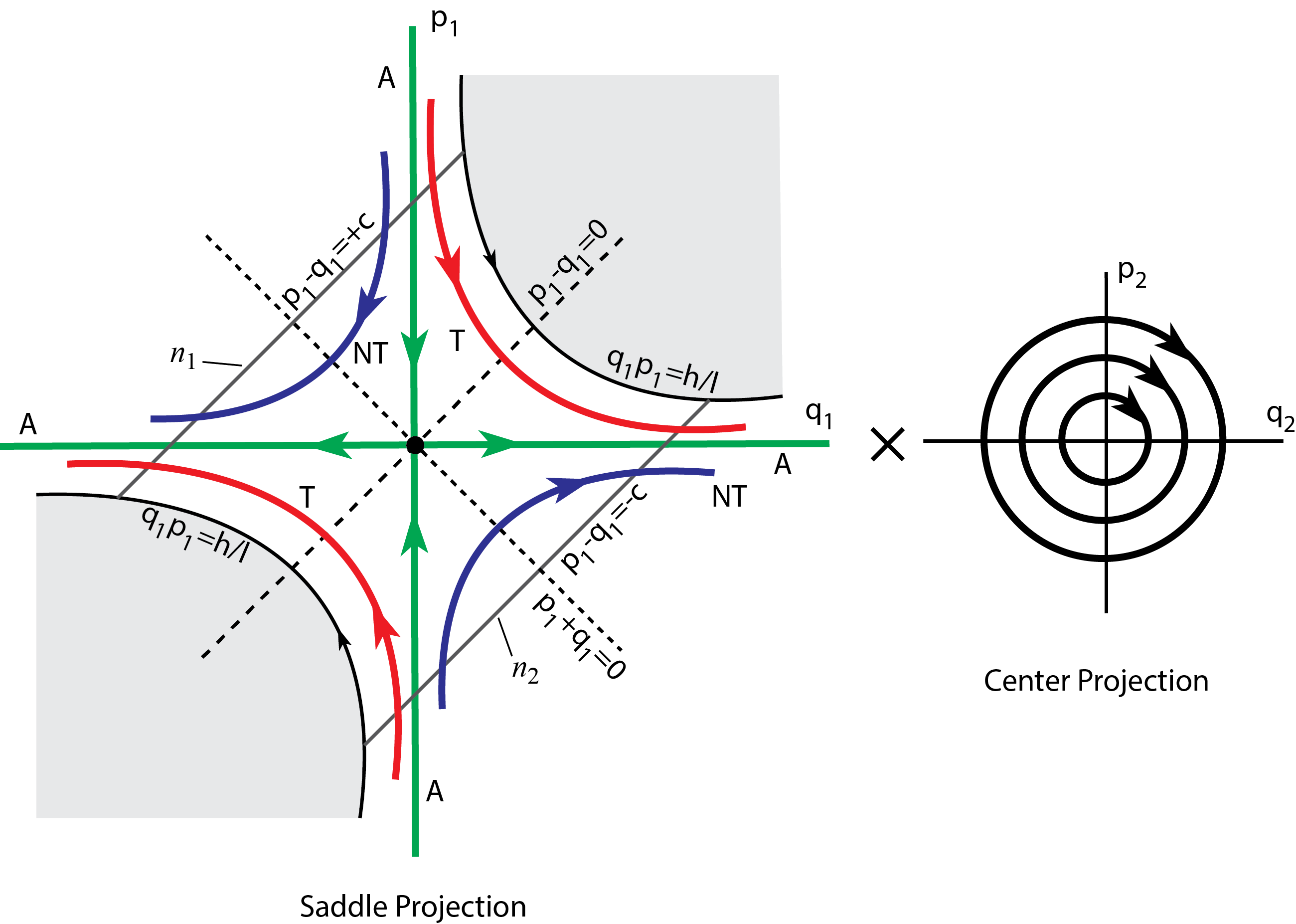
Figure 3: The flow in the equilibrium region has the form saddle $\times$ center. On the left is shown the projection onto the $(p_{1},q_{1})$ plane, the saddle projection. For the conservative dynamics, the Hamiltonian function $\mathcal{H}_{2}$ remains constant at $h>0$. Shown are the periodic orbit (black dot at the center), the asymptotic orbits (labeled A), two transit orbits (T) and two non-transit orbits (NT).

We call the set of points on each bounding 2-sphere where $q_{1}+p_{1}=0$ the equator, and the sets where $q_{1}+p_{1}>0$ or $q_{1}+p_{1}<0$ will be called the northern and southern hemispheres, respectively.

The Linear Flow in $\mathcal{R}$

To analyze the flow in $\mathcal{R}$, consider the projections on the ($q_{1},p_{1}$)-plane and the $(q_{2},p_{2})$-plane, respectively. In the first case we see the standard picture of a saddle point in two dimensions, and in the second, of a center consisting of harmonic oscillator motion. Figure 3 schematically illustrates the flow. With regard to the first projection we see that $\mathcal{R}$ itself projects to a set bounded on two sides by the hyperbola $q_{1}p_{1}=h/\lambda$ (corresponding to $q_{2}^{2}+p_{2}^{2}=0$, see (47)) and on two other sides by the line segments $p_{1}-q_{1}=\pm c$, which correspond to the bounding 2-spheres, $n_{1}$ and $n_{2}$, respectively.

Since $q_{1}p_{1}$ is an integral of the equations in $\mathcal{R}$, the projections of orbits in the $(q_{1},p_{1})$-plane move on the branches of the corresponding hyperbolas $q_{1}p_{1}=$ constant, except in the case $q_{1}p_{1}=0$, where $q_{1}=0$ or $p_{1}=0$. If $q_{1}p_{1}>0$, the branches connect the bounding line segments $p_{1}-q_{1}=\pm c$ and if $q_{1}p_{1}<0$, they have both end points on the same segment. A check of equation (48) shows that the orbits move as indicated by the arrows in Figure 3.

To interpret Figure 3 as a flow in $\mathcal{R}$, notice that each point in the $(q_{1},p_{1})$-plane projection corresponds to a 1-sphere $S^{1}$ in $\mathcal{R}$ given by

$$q_{2}^{2}+p_{2}^{2}=\tfrac{2}{\omega_{p}}(h-\lambda q_{1}p_{1}).$$

Of course, for points on the bounding hyperbolic segments ($q_{1}p_{1}=h/\lambda$), the 1-sphere collapses to a point. Thus, the segments of the lines $p_{1}-q_{1}=\pm c$ in the projection correspond to the 2-spheres bounding $\mathcal{R}$. This is because each corresponds to a 1-sphere crossed with an interval where the two end 1-spheres are pinched to a point.

We distinguish nine classes of orbits grouped into the following four categories:

1. The point $q_{1}=p_{1}=0$ corresponds to an invariant 1-sphere $S^{1}_{h}$, an unstable period orbit in $\mathcal{R}$. This 1-sphere is given by

   $$q_{2}^{2}+p_{2}^{2}=\tfrac{2}{\omega_{p}}h,\hskip 21.68121ptq_{1}=p_{1}=0.$$ (53)

   It is an example of a normally hyperbolic invariant manifold (NHIM) (see [24]). Roughly, this means that the stretching and contraction rates under the linearized dynamics transverse to the 1-sphere dominate those tangent to the 1-sphere. This is clear for this example since the dynamics normal to the 1-sphere are described by the exponential contraction and expansion of the saddle point dynamics. Here the 1-sphere acts as a “big saddle point”. See the black dot at the center of the $(q_{1},p_{1})$-plane on the left side of Figure 3.

2. The four half open segments on the axes, $q_{1}p_{1}=0$, correspond to four cylinders of orbits asymptotic to this invariant 1-sphere $S^{1}_{h}$ either as time increases ($p_{1}=0$) or as time decreases ($q_{1}=0$). These are called asymptotic orbits and they form the stable and the unstable manifolds of $S^{1}_{h}$. The stable manifolds, $W^{s}_{\pm}(S^{1}_{h})$, are given by

   $$q_{2}^{2}+p_{2}^{2}=\tfrac{2}{\omega_{p}}h,\hskip 21.68121ptq_{1}=0,\hskip 21.68121ptp_{1}~{}{\rm arbitrary}.$$ (54)

   $W^{s}_{+}(S^{1}_{h})$ (with $p_{1}>0$) is the branch going entering from $n_{1}$ and $W^{s}_{-}(S^{1}_{h})$ (with $p_{1}<0$) is the branch going entering from $n_{2}$. The unstable manifolds, $W^{u}_{\pm}(S^{1}_{h})$, are given by

   $$q_{2}^{2}+p_{2}^{2}=\tfrac{2}{\omega_{p}}h,\hskip 21.68121ptp_{1}=0,\hskip 21.68121ptq_{1}~{}{\rm arbitrary}$$ (55)

   $W^{u}_{+}(S^{1}_{h})$ (with $q_{1}>0$) is the branch exiting from $n_{2}$ and $W^{u}_{-}(S^{1}_{h})$ (with $q_{1}<0$) is the branch exiting from $n_{1}$. See the four orbits labeled A of Figure 3.

3. The hyperbolic segments determined by $q_{1}p_{1}={\rm constant}>0$ correspond to two cylinders of orbits which cross $\mathcal{R}$ from one bounding 2-sphere to the other, meeting both in the same hemisphere; the northern hemisphere if they go from $p_{1}-q_{1}=+c$ to $p_{1}-q_{1}=-c$, and the southern hemisphere in the other case. Since these orbits transit from one realm to another, we call them transit orbits. See the two orbits labeled T of Figure 3.

4. Finally the hyperbolic segments determined by $q_{1}p_{1}={\rm constant}<0$ correspond to two cylinders of orbits in $\mathcal{R}$ each of which runs from one hemisphere to the other hemisphere on the same bounding 2-sphere. Thus if $q_{1}>0$, the 2-sphere is $n_{1}$ ($p_{1}-q_{1}=-c$) and orbits run from the southern hemisphere ($q_{1}+p_{1}<0$) to the northern hemisphere ($q_{1}+p_{1}>0$) while the converse holds if $q_{1}<0$, where the 2-sphere is $n_{2}$. Since these orbits return to the same realm, we call them non-transit orbits. See the two orbits labeled NT of Figure 3.

3.3 Trajectories in the neck region

We now examine the appearance of the orbits in configuration space, that is, in $(\bar{q}_{1},\bar{q}_{2})$-plane. In configuration space, $\mathcal{R}$ appears as the neck region connecting two realms, so trajectories in $\mathcal{R}$ will be transformed back to the neck region. It should pointed out that at each moment in time, all trajectories must evolve within the energy boundaries which are zero velocity curves (corresponding to $\bar{p}_{1}=\bar{p}_{2}=0$) given by solving (37) for $\bar{q}_{2}$ as a function of $\bar{q}_{1}$,

$$\bar{q}_{2}(\bar{q}_{1})=\frac{\bar{q}_{1}\pm\sqrt{\bar{q}_{1}^{2}-2c_{y}(h+\tfrac{c_{x}}{2}\bar{q}_{1}^{2})}}{c_{y}}$$

Recall that in order to obtain the analytical solutions for $\bar{z}=(\bar{q}_{1},\bar{q}_{2},\bar{p}_{1},\bar{p}_{2})$, system $\bar{z}$ has been transformed into system $z=(q_{1},q_{2},p_{1},p_{2})$ by using the symplectic matrix $C$ consisting of generalized (re-scaled) eigenvectors $u_{+\lambda},u_{-\lambda},u_{\omega_{p}},v_{\omega_{p}}$ with corresponding eigenvalues $\pm\lambda$ and $\pm i\omega_{p}$. Thus, the system $z$ should be transformed back to system $\bar{z}$ which generates the following general (real) solution with the form

$$\begin{split}\bar{z}(t)=\left(\bar{q}_{1},\bar{q}_{2},\bar{p}_{1},\bar{p}_{2}\right)^{T}=q_{1}^{0}e^{\lambda t}u_{+\lambda}+p_{1}^{0}e^{-\lambda t}u_{-\lambda}+\mathrm{Re}\left[\beta_{0}e^{-i\omega_{p}t}\left(u_{\omega_{p}}-iv_{\omega_{p}}\right)\right]\end{split}$$ (56)

where $q_{1}^{0},p_{1}^{0}$ are real and $\beta_{0}=q_{2}^{0}+ip_{2}^{0}$ is complex.

Upon inspecting this general solution, we see that the solutions on the energy surface fall into different classes depending upon the limiting behaviors of $\bar{q}_{1},\bar{q}_{2}$ as $t$ tends to plus or minus infinity. Notice that

$$\begin{split}\bar{q}_{1}(t)&=\frac{q_{1}^{0}}{s_{1}}e^{\lambda t}-\frac{p_{1}^{0}}{s_{1}}e^{-\lambda t}+\frac{1}{s_{2}}\left(q_{2}^{0}\cos\omega_{p}t+p_{2}^{0}\sin\omega_{p}t\right)\\ \bar{q}_{2}(t)&=\frac{c_{x}-\lambda^{2}}{s_{1}}q_{1}^{0}e^{\lambda t}+\frac{\lambda^{2}-c_{x}}{s_{1}}p_{1}^{0}e^{-\lambda t}+\frac{\omega_{p}^{2}+c_{x}}{s_{2}}\left(q_{2}^{0}\cos\omega_{p}t+p_{2}^{0}\sin\omega_{p}t\right)\\ \end{split}$$ (57)

Thus, if $t\rightarrow+\infty$, then $\bar{q}_{1}(t)$ is dominated by its $q_{1}^{0}$ term. Hence, $\bar{q}_{1}(t)$ tends to minus infinity (staying on the left-hand side), is bounded (staying around the equilibrium point), or tends to plus infinity (staying on the right-hand side) according to $q_{1}^{0}<0$, $q_{1}^{0}=0$ and $q_{1}^{0}>0$. See Figure 4. The same statement holds if $t\rightarrow-\infty$ and $-p_{1}^{0}$ replaces $q_{1}^{0}$. Different combinations of the signs of $q_{1}^{0}$ and $p_{1}^{0}$ will give us again the same nine classes of orbits which can be grouped into the same four categories.

1. If $q_{1}^{0}=p_{1}^{0}=0$, we obtain a periodic solution. The periodic orbit projects onto the $(\bar{q}_{1},\bar{q}_{2})$ plane as a line with the following expression

   $$\begin{split}\bar{q}_{1}&=\frac{1}{s_{2}}\left(q_{2}^{0}\cos\omega_{p}t+p_{2}^{0}\sin\omega_{p}t\right)\\ \bar{q}_{2}&=\frac{\omega_{p}^{2}+c_{x}}{s_{2}}\left(q_{2}^{0}\cos\omega_{p}t+p_{2}^{0}\sin\omega_{p}t\right)\\ &=\left(\omega_{p}^{2}+c_{x}\right)\bar{q}_{1}\end{split}$$ (58)

   Notice (47) and $\mathcal{H}_{2}$ now can be rewritten as $\mathcal{H}_{2}=\omega_{p}|\beta_{0}|^{2}/2$. Thus, since $\mathcal{H}_{2}=h$, the length of the periodic orbit is $\sqrt{2h\left[(\omega_{p}^{2}+c_{x})^{2}+1\right]/\left(\omega_{p}s_{2}^{2}\right)}$. Note that the length of the line goes to zero with $h$.

2. Orbits with $q_{1}^{0}p_{1}^{0}=0$ are asymptotic orbits. They are asymptotic to the periodic orbit.

   1. When $q_{1}^{0}=0$ , the general solutions for $\bar{q}_{1},\bar{q}_{2}$ are

      $$\begin{split}\bar{q}_{1}&=-\frac{p_{1}}{s_{1}}+\frac{q_{2}}{s_{2}}\\ \bar{q}_{2}&=\frac{\lambda^{2}-c_{x}}{s_{1}}p_{1}+\frac{\omega_{p}^{2}+c_{x}}{s_{2}}q_{2}\\ &=\left(c_{x}-\lambda^{2}\right)\bar{q}_{1}+\frac{\lambda^{2}+\omega_{p}^{2}}{s_{2}}\left(q_{2}^{0}\cos\omega_{p}t+p_{2}^{0}\sin\omega_{p}t\right)\end{split}$$ (59)

      Thus, the orbits with $q_{1}^{0}=0$ project into a strip $S$ in the $(\bar{q}_{1},\bar{q}_{2})$-plane bounded by

      $$\begin{split}\bar{q}_{2}=\left(c_{x}-\lambda^{2}\right)\bar{q}_{1}\pm\frac{\lambda^{2}+\omega_{p}^{2}}{s_{2}}\sqrt{\frac{2h}{\omega_{p}}}\end{split}$$ (60)

   2. For $p_{1}^{0}=0$, following the same procedure as $q_{1}^{0}=0$, we have

      $$\begin{split}\bar{q}_{1}&=\frac{q_{1}}{s_{1}}+\frac{q_{2}}{s_{2}}\\ \bar{q}_{2}&=\left(c_{x}-\lambda^{2}\right)\bar{q}_{1}+\frac{\lambda^{2}+\omega_{p}^{2}}{s_{2}}\left(q_{2}^{0}\cos\omega_{p}t+p_{2}^{0}\sin\omega_{p}t\right)\end{split}$$ (61)

      Notice that these two asymptotic orbits with $q_{1}^{0}=0$ and $p_{1}^{0}=0$ share the same strip $S$ and the same boundaries governed by (60). Also, since the slopes of the periodic orbit and the strip satisfies $\left(c_{x}-\lambda^{2}\right)\left(c_{x}+\omega_{p}^{2}\right)=-1$, the periodic orbit is perpendicular to the strip. In other words, the length of the periodic orbit is exactly the same as the width of the strip.

3. Orbits with $q_{1}^{0}p_{1}^{0}>0$ are transit orbits because they cross the equilibrium region $R$ from $-\infty$ (the left-hand side) to $+\infty$ (the right-hand side) or vice versa.

4. Orbits with $q_{1}^{0}p_{1}^{0}<0$ are non-transit orbits

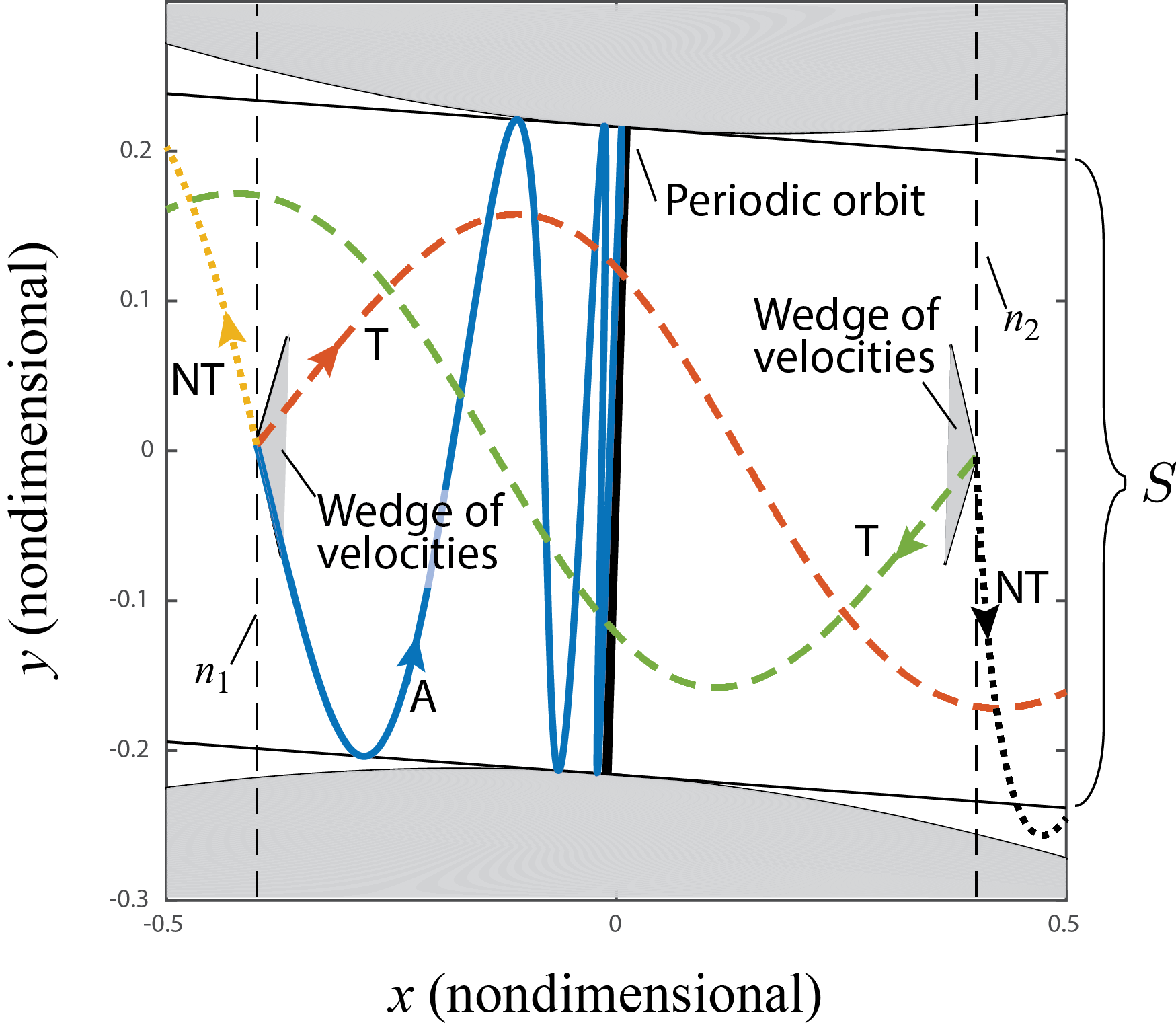
Figure 4: The flow of the conservative system in $\mathcal{R}$, the equilibrium region projected onto the $xy$ configuration space, for a fixed value of energy, $\mathcal{H}_{2}=h>0$. For any point on the bounding vertical lines $n_{1}$ or $n_{2}$ (dashed), there is a wedge of velocity directions inside of which the trajectories are transit orbits, and outside of which are non-transit orbits. The boundary of the wedge gives the orbits asymptotic to the single unstable periodic orbit in the neck for this energy. Shown are a typical asymptotic orbit; two transit orbits (dashed); and two non-transit orbits (dotted).

To study the flow in position space, Figure 4 gives the four categories of orbits. From (LABEL:conser-sol), we can see that for transit orbits and non-transit orbits, the signs of $q_{1}^{0}p_{1}^{0}$ must satisfy $q_{1}^{0}p_{1}^{0}>0$ and $q_{1}^{0}p_{1}^{0}<0$,respectively.

In Figure 4, $S$ is the strip mentioned above. Outside of the strip, the signs of $q_{1}^{0}$ and $p_{1}^{0}$ are independent of the direction of the velocity. These signs can be determined in each of the components of the equilibrium region $\mathcal{R}$ complementary to the strip. For example, in the left two components, $q_{1}^{0}<0$ and $p_{1}^{0}>0$, while in the right two components $q_{1}^{0}>0$ and $p_{1}^{0}<0$. Therefore, $q_{1}^{0}p_{1}^{0}<0$ in all components and only non-transit orbits project on to these four components.

Inside the strip the situation is more complicated since in $S$ the signs of $q_{1}^{0}$ and $p_{1}^{0}$ depend on the direction of the velocity. At each position $(\bar{q}_{1},\bar{q}_{2})$ inside the strip there exists the so-called ‘wedge’ of velocities in which $q_{1}^{0}p_{1}^{0}>0$ which was first found by Conley (1968) [10] in the restricted three-body problem. See the shaded wedges in Figure 4. The existence and the angle of the wedge of velocity will be given in the next part. For simplicity we have indicated this dependence only on the two vertical bounding line segments in Figure 4. For example, consider the intersection of strip $S$ with left-most vertical line. On the subsegment so obtained there is at each point a wedge of velocity in which both $q_{1}^{0}$ and $p_{1}^{0}$ are positive, so that orbits with velocity interior to the wedge are transit orbits $(q_{1}^{0}p_{1}^{0}>0)$. Of course, orbits with velocity on the boundary ot the wedge are asymptotic $(q_{1}^{0}p_{1}^{0}=0)$, while orbits with velocity outside of the wedge are non-transit. The situation on the other subsegment is similar.

The wedge of velocities

To establish the wedge of velocity and obtain its angle, we need to use the following fact that all the inner products of one generalized eigenvector and another generalized eigenvector associated with $B$ are zero except for

$$\begin{split}u_{+\lambda}^{T}Bu_{-\lambda}&=u_{-\lambda}^{T}Bu_{+\lambda}=\lambda\\ u_{\omega_{p}}^{T}Bu_{\omega_{p}}&=v_{\omega_{p}}^{T}Bv_{\omega_{p}}=\omega_{p}\\ \end{split}$$ (62)

Using this condition, we have the following relations, as

$$\begin{split}\lambda&=u_{+\lambda}^{T}Bu_{-\lambda}\\ \Rightarrow\lambda q_{1}^{0}&=q_{1}^{0}u_{+\lambda}^{T}Bu_{-\lambda}\\ \Rightarrow\lambda q_{1}^{0}&=e^{-\lambda t}\left(q_{1}^{0}e^{\lambda t}u_{+\lambda}\right)^{T}Bu_{-\lambda}\\ \Rightarrow\lambda q_{1}^{0}&=e^{-\lambda t}\bar{z}^{T}Bu_{-\lambda}\\ \Rightarrow\lambda q_{1}^{0}&=e^{-\lambda t}\left(\frac{\lambda^{2}}{s_{1}}\bar{q}_{1}-\frac{1-c_{x}c_{y}+c_{y}\lambda^{2}}{s_{1}}\bar{q}_{2}+\frac{\lambda}{s_{1}}\bar{p}_{1}+\frac{c_{x}\lambda-\lambda^{3}}{s_{1}}\bar{p}_{2}\right)\end{split}$$ (63)

Using similar arguments, we can also obtain

$$\begin{split}\lambda p_{1}^{0}&=e^{\lambda t}\left(-\frac{\lambda^{2}}{s_{1}}\bar{q}_{1}+\frac{1-c_{x}c_{y}+c_{y}\lambda^{2}}{s_{1}}\bar{q}_{2}+\frac{\lambda}{s_{1}}\bar{p}_{1}+\frac{c_{x}\lambda-\lambda^{3}}{s_{1}}\bar{p}_{2}\right)\end{split}$$ (64)

Thus, we obtain the following relations

$$\begin{split}\lambda q_{1}^{0}e^{\lambda t}&=\frac{\lambda^{2}}{s_{1}}\bar{q}_{1}-\frac{1-c_{x}c_{y}+c_{y}\lambda^{2}}{s_{1}}\bar{q}_{2}+\frac{\lambda}{s_{1}}\bar{p}_{1}+\frac{c_{x}\lambda-\lambda^{3}}{s_{1}}\bar{p}_{2}\\ \lambda p_{1}^{0}e^{-\lambda t}&=-\frac{\lambda^{2}}{s_{1}}\bar{q}_{1}+\frac{1-c_{x}c_{y}+c_{y}\lambda^{2}}{s_{1}}\bar{q}_{2}+\frac{\lambda}{s_{1}}\bar{p}_{1}+\frac{c_{x}\lambda-\lambda^{3}}{s_{1}}\bar{p}_{2}\end{split}$$ (65)

Let $\chi$ be the angles determined by

$$\begin{split}\cos\chi&=\frac{1}{\sqrt{\left(\lambda^{2}-c_{x}\right)^{2}+1}},\ \ \ \ \ \ \sin\chi=\frac{\lambda^{2}-c_{x}}{\sqrt{\left(\lambda^{2}-c_{x}\right)^{2}+1}}.\\ \end{split}$$ (66)

Furthermore, let

$$\begin{split}\bar{p}_{1}=\rho\cos\theta,\ \ \ \bar{p}_{2}=\rho\sin\theta\end{split}$$ (67)

and

$$\begin{split}\gamma&=\left(\frac{\lambda^{2}}{s_{1}}\bar{q}_{1}-\frac{1-c_{x}c_{y}+c_{y}\lambda^{2}}{s_{1}}\bar{q}_{2}\right)\left[\frac{\lambda^{2}}{s_{1}^{2}}\left(\bar{p}_{1}^{2}+\bar{p}_{2}^{2}\right)\left(\left(\lambda^{2}-c_{x}\right)^{2}+1\right)\right]^{-\frac{1}{2}}\\ \end{split}$$ (68)

Using (LABEL:gamma), (65) can be rewritten as

$$\begin{split}\lambda q_{1}^{0}e^{\lambda t}\left[\frac{\lambda^{2}}{s_{1}^{2}}\left(\bar{p}_{1}^{2}+\bar{p}_{2}^{2}\right)\left(\left(\lambda^{2}-c_{x}\right)^{2}+1\right)\right]^{-\frac{1}{2}}&=\gamma+\cos(\theta-\chi)\\ \lambda p_{1}^{0}e^{-\lambda t}\left[\frac{\lambda^{2}}{s_{1}^{2}}\left(\bar{p}_{1}^{2}+\bar{p}_{2}^{2}\right)\left(\left(\lambda^{2}-c_{x}\right)^{2}+1\right)\right]^{-\frac{1}{2}}&=-\gamma+\cos(\theta-\chi)\end{split}$$ (69)

So far, the signs of $q_{1}^{0}$ and $p_{1}^{0}$ can be determined using Eq. (69). From Eq. (69), it can be concluded that $\gamma$ is only dependent on the position $(\bar{q}_{1},\bar{q}_{2})$, because $\bar{p}_{1}^{2}+\bar{p}_{2}^{2}$ can be obtained from Eq. (37) once the position is given. Outside the strip, we have $\mid\gamma\mid>1$. In this case, the signs of $q_{1}^{0}$ and $p_{1}^{0}$ are independent of the direction of velocity and are always opposite, which makes $q_{1}^{0}p_{1}^{0}<0$. Thus, only non-transit orbit exist in these regions. Inside the strip, we have $\mid\gamma\mid<1$. This situation is quite different since the signs of $q_{1}^{0}$ and $p_{1}^{0}$ are dependent on the angle of velocity. Because for transit orbits, the sign of $q_{1}^{0}p_{1}^{0}$ must be positive. Thus, we can vary $\theta$ (the direction of velocity) to satisfy this condition, and the wedge of velocity can be determined. It should be noted that the wedge of velocity can only exist inside the strip $S$: outside of $S$, no transit orbit exists.

4 Linearized Dissipative Hamiltonian System

4.1 Solutions near the equilibria

For the dissipative system, we still use the symplectic matrix $C$ as in (46) to transform to the eigenbasis, i.e., transform $\bar{z}=(\bar{q}_{1},\bar{q}_{2},\bar{p}_{1},\bar{p}_{2})$ to $z=(q_{1},q_{2},p_{1},p_{2})$. The equations of motion now become

$$\dot{z}=\Lambda z+\Delta z$$ (70)

where $\Lambda={C}^{-1}{{A}}{C}$ from before and the transformed damping matrix is,

$$\begin{split}\Delta={C}^{-1}{{D}}{C}=-c_{1}\left(\begin{array}[]{rrrr}\tfrac{1}{2}&0&\tfrac{1}{2}&0\\ 0&0&0&0\\ \tfrac{1}{2}&0&\tfrac{1}{2}&0\\ 0&0&0&1\end{array}\right)\end{split}$$ (71)

which results in

$$\begin{cases}\dot{q}_{1}=\left(\lambda-\frac{c_{1}}{2}\right)q_{1}-\frac{c_{1}}{2}p_{1}\\ \dot{p}_{1}=-\frac{c_{1}}{2}q_{1}+\left(-\lambda-\frac{c_{1}}{2}\right)p_{1}\end{cases}$$ (72a)

$$\begin{cases}\dot{q}_{2}=\omega_{p}p_{2}\\ \dot{p}_{2}=-\omega_{p}q_{2}-c_{1}p_{2}\end{cases}$$ (72b)

Notice that the dynamics on the $(q_{1},p_{1})$ plane and $(q_{2},p_{2})$ plane are uncoupled.

The fourth-order characteristic polynomial is thus decomposable into $p(\beta)=p_{1}(\beta)p_{2}(\beta)$, where the second-order characteristic polynomials for (72a) and (72b) are

$$p_{1}(\beta)=\beta^{2}+c_{1}\beta-\lambda^{2}$$ (73a)

$$p_{2}(\beta)=\beta^{2}+c_{1}\beta+\omega_{p}^{2}$$ (73b)

Considering $c_{1}$ is positive and $c_{1}^{2}$ is smaller compared with $4\omega_{p}^{2}$, the determinants for (73) are

$$\Delta_{1}=c_{1}^{2}+4\lambda^{2}>0$$ (74a)

$$\Delta_{2}=c_{1}^{2}-4\omega_{p}^{2}<0$$ (74b)

The corresponding eigenvalues are

$$\begin{cases}\beta_{1}=\frac{-c_{1}+\sqrt{c_{1}^{2}+4\lambda^{2}}}{2}\\ \beta_{2}=\frac{-c_{1}-\sqrt{c_{1}^{2}+4\lambda^{2}}}{2}\end{cases}$$ (75a)

$$\begin{cases}\beta_{3}=-\delta+i\omega_{d}\\ \beta_{4}=-\delta-i\omega_{d}\\ \end{cases}$$ (75b)

where $\delta=\frac{c_{1}}{2},\omega_{d}=\omega_{p}\sqrt{1-\xi_{d}^{2}}$ and $\xi_{d}=\frac{\delta}{\omega_{p}}$, with the corresponding eigenvectors

$$\begin{split}u_{\beta_{1}}&=\left(\frac{c_{1}}{2},\lambda-\frac{1}{2}\sqrt{c_{1}^{2}+4\lambda^{2}}\right)\\ u_{\beta_{2}}&=\left(\frac{c_{1}}{2},\lambda+\frac{1}{2}\sqrt{c_{1}^{2}+4\lambda^{2}}\right)\\ u_{\beta_{3}}&=\left(\omega_{p},-\delta+i\omega_{d}\right)\\ u_{\beta_{4}}&=\left(\omega_{p},-\delta-i\omega_{d}\right)\end{split}$$ (76)

Thus, the general solutions for the $\left(q_{1},p_{1}\right)$ and $\left(q_{2},p_{2}\right)$ systems are

$$\begin{cases}q_{1}=k_{1}e^{\beta_{1}t}+k_{2}e^{\beta_{2}t}\\ p_{1}=k_{3}e^{\beta_{1}t}+k_{4}e^{\beta_{2}t}\end{cases}$$ (77a)

$$\begin{cases}q_{2}=k_{5}e^{-\delta t}\cos{\omega_{d}t}+k_{6}e^{-\delta t}\sin{\omega_{d}t}\\ p_{2}=\frac{k_{5}}{\omega_{p}}e^{-\delta t}\left(-\delta\cos{\omega_{d}t}-\omega_{d}\sin{\omega_{d}t}\right)+\frac{k_{6}}{\omega_{p}}e^{-\delta t}\left(\omega_{d}\cos{\omega_{d}t-\delta\sin{\omega_{d}t}}\right)\\ \end{cases}$$ (77b)

where

$$\begin{split}k_{1}&=\frac{q_{1}^{0}\left(2\lambda+\sqrt{c_{1}^{2}+4\lambda^{2}}\right)-c_{1}p_{1}^{0}}{2\sqrt{c_{1}^{2}+4\lambda^{2}}},\hskip 36.135ptk_{2}=\frac{q_{1}^{0}\left(-2\lambda+\sqrt{c_{1}^{2}+4\lambda^{2}}\right)+c_{1}p_{1}^{0}}{2\sqrt{c_{1}^{2}+4\lambda^{2}}},\\ k_{3}&=\frac{p_{1}^{0}\left(-2\lambda+\sqrt{c_{1}^{2}+4\lambda^{2}}\right)-c_{1}q_{1}^{0}}{2\sqrt{c_{1}^{2}+4\lambda^{2}}},\hskip 36.135ptk_{4}=\frac{p_{1}^{0}\left(2\lambda+\sqrt{c_{1}^{2}+4\lambda^{2}}\right)+c_{1}q_{1}^{0}}{2\sqrt{c_{1}^{2}+4\lambda^{2}}},\\ k_{5}&=q^{0}_{2},\hskip 36.135ptk_{6}=\frac{p^{0}_{2}\omega_{p}+q^{0}_{2}\delta}{\omega_{d}}\end{split}$$

Note that $k_{1}=q_{1}^{0}$, $k_{4}=p_{1}^{0}$, $k_{2}=k_{3}=0$, $k_{5}=q_{2}^{0}$ and $k_{6}=p_{2}^{0}$ if $c_{1}=c_{2}=0$.

Taking total derivative with respect to $t$ of the Hamiltonian along trajectories gives us

$$\begin{split}\frac{d\mathcal{H}_{2}}{dt}=-\tfrac{1}{2}c_{1}\lambda\left(q_{1}+p_{1}\right)^{2}-c_{1}\omega_{p}p_{2}^{2}\leq 0\end{split}$$ (78)

which means the Hamiltonian is non-increasing, and will generally decrease due to damping.

4.2 Boundary of transit and non-transit orbits

The Linear Flow in $\mathcal{R}$

Similar to the discussions for the conservative system, we still choose an equilibrium region $\mathcal{R}$ bounded by regions which project to the lines $n_{1}$ and $n_{2}$ in the $(q_{1},p_{1})$-plane (see Figure 5). To analyze the flow in $\mathcal{R}$, we consider the projections on the $(q_{1},p_{1})$-plane and the $(q_{2},p_{2})$-plane, respectively. In the first case we see the standard picture of saddle point, now rotated compared to the conservative case, and in the second, of a stable focus which is a damped oscillator with frequency $\omega_{d}=\omega_{p}\sqrt{1-\xi_{d}^{2}}$, where $\xi_{d}=\frac{c_{1}}{2\omega_{p}}$ - the viscous damping factor (damping ralative to critical damping). Notice that the frequency $\omega_{d}$ for the damped system decreases with increased damping, but only very slightly for lightly damped systems.

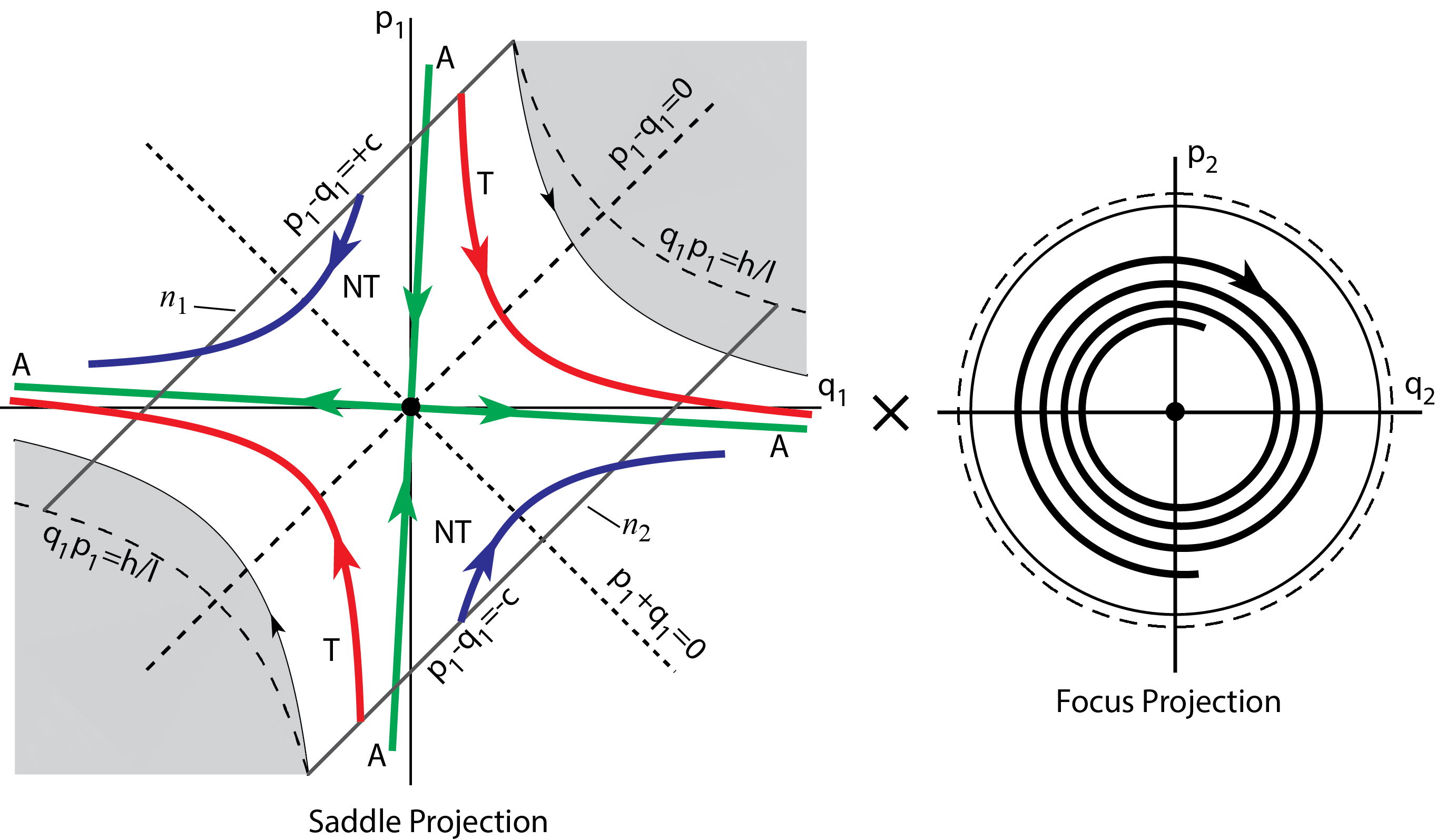
Figure 5: The flow in the equilibrium region around S₁ for the dissipative system has the form saddle $\times$ focus. On the left is shown the projection onto the $(p_{1},q_{1})$ plane, the saddle projection. The asymptotic orbits (labeled A) on this projection are the saddle-type asymptotic orbits, and are rotated clockwise compared to the conservative system. They still form the separatrix between transit orbits (T) and two non-transit orbits (NT). The black dot at the center represents trajectories with only a focus projection, thus oscillatory dynamics decaying onto the point S₁. As the energy, the Hamiltonian function $\mathcal{H}_{2}$, is decreasing, the boundary is no longer equal to $q_{1}p_{1}=h/\lambda$, as it is for the conservative case, where $\mathcal{H}_{2}=h$ is the initial value of the energy for those trajectories entering through the left or right side bounding sphere (i.e., $n_{1}$ or $n_{2}$, respectively). These boundaries (the boundary of the shaded region) still correspond to the fastest trajectories through the neck region for a given $h$.

We distinguish nine classes of orbits grouped into the following four categories:

1. The point $q_{1}=p_{1}=0$ corresponds to a focus-type asymptotic orbit with motion purely in the $(q_{2},p_{2})$-plane (see black dot at the origin of the $(q_{1},p_{1})$-plane in Figure 5). Such orbits are asymptotic to the equilibrium point S₁ itself. Due to the effect of damping, the periodic orbit in the conservative system, which is an invariant 1-sphere $S_{h}^{1}$ mentioned in (53), does not exist.

2. The four half open segments on the lines governed by $q_{1}=c_{1}p_{1}/(2\lambda\pm\sqrt{c_{1}^{2}+4\lambda^{2}})$ correspond to saddle-type asymptotic orbits. See the four orbits labeled A in Figure 5. These orbits have motion in both the $(q_{1},p_{1})$- and $(q_{2},p_{2})$-planes.

3. The segments which cross $\mathcal{R}$ from one boundary to the other, i.e., from $p_{1}-q_{1}=+c$ to $p_{1}-q_{1}=-c$ in the northern hemisphere, and vice versa in the southern hemisphere, correspond to transit orbits. See the two orbits labeled $T$ of Figure 5.

4. Finally the segments which run from one hemisphere to the other hemisphere on the same boundary, namely which start from $p_{1}-q_{1}=\pm c$ and return to the same boundary, correspond to non-transit orbits. See the two orbits labeled NT of Figure 5.

4.3 Trajectories in the neck region

Following the same procedure of analysis as for conservative system, the general solution to the dissipative system can be obtained by $\bar{z}=Cz$ which gives

$$\begin{split}\bar{q}_{1}&=\frac{k_{1}-k_{3}}{s_{1}}e^{\beta_{1}t}-\frac{k_{4}-k_{2}}{s_{1}}e^{\beta_{2}t}+\frac{q_{2}}{s_{2}}\\ \bar{q}_{2}&=\frac{k_{1}-k_{3}}{s_{1}}(c_{x}-\lambda^{2})e^{\beta_{1}t}-\frac{k_{4}-k_{2}}{s_{1}}(c_{x}-\lambda^{2})e^{\beta_{2}t}+\frac{\omega_{p}^{2}+c_{x}}{s_{2}}q_{2}\end{split}$$ (79)

Similar to the situation in the conservative system, the solutions for the dissipative system on the energy surface fall into different classes depending upon the limiting behaviors. See Figure 6.

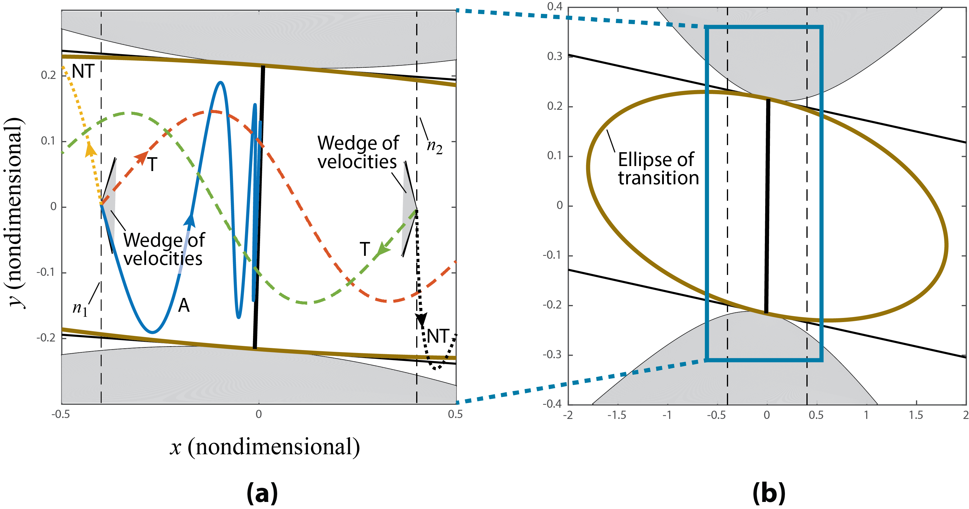
Figure 6: The flow of the dissipative system in $\mathcal{R}$, the equilibrium region projected onto the $xy$ configuration space, for trajectories starting at a fixed value of energy, $\mathcal{H}_{2}=h$, on either the right or left side vertical boundaries. As before, for any point on a bounding vertical line (dashed), there is a wedge of velocities inside of which the trajectories are transit orbits, and outside of which are non-transit orbits. For a given fixed energy, the wedge for the dissipative system is a subset of the wedge for the conservative system. The boundary of the wedge gives the orbits asymptotic (saddle-type) to the equilibrium point S₁.

From (79) we know that the conditions $k_{1}-k_{3}>0$, $k_{1}-k_{3}=0$ and $k_{1}-k_{3}<0$ make $\bar{q}_{1}$ tend to minus infinity, are bounded or tend to plus infinity if $t\rightarrow\infty$. See Figure 5. The same statement holds if $t\rightarrow-\infty$ and $k_{2}-k_{4}$ replaces $k_{1}-k_{3}$. Nine classes of orbits can be given according to different combinations of the sign of $k_{1}-k_{3}$ and $k_{2}-k_{4}$ which can be classified into the following four categories:

1. Orbits with $k_{1}-k_{3}=k_{4}-k_{2}=0$ are focus-type asymptotic orbits

   $$\begin{split}\bar{q}_{1}=q_{2}/s_{2},\hskip 36.135pt\bar{q}_{2}=\left(\omega_{p}^{2}+c_{x}\right)\bar{q}_{1}\end{split}$$ (80)

   Notice the presence of $q_{2}$ in (77) reveals that the amplitude of the periodic orbit will gradually decease at the rate of $e^{-\delta t}$ with time. The larger the damping, the faster the rate will be.

2. Orbits with $\left(k_{1}-k_{3}\right)\left(k_{4}-k_{2}\right)=0$ are saddle-type asymptotic orbits

   $$\bar{q}_{2}=\left(c_{x}-\lambda^{2}\right)\bar{q}_{1}+\frac{\lambda^{2}+\omega_{p}^{2}}{s_{2}}q_{2}$$ (81)

   In similarity with the shrinking of the length of the periodic orbit, the amplitude of asymptotic orbits are also shrinking.

3. Orbits with $\left(k_{1}-k_{3}\right)\left(k_{4}-k_{2}\right)>0$ are transit orbits

4. Orbits with $\left(k_{1}-k_{3}\right)\left(k_{4}-k_{2}\right)<0$ are non-transit orbits

Wedge of velocities

We previously obtained the wedge of velocities for the conservative system. However, this method is no longer effective for the dissipative system. Thus, another approach will be pursued here.

Based on the eigenvectors in (76), we can conclude that the directions of stable asymptotic orbits are along $u_{\beta_{2}}=\left(\frac{c_{1}}{2},\lambda+\frac{1}{2}\sqrt{c_{1}^{2}+4\lambda^{2}}\right)$. In this case, all asymptotic orbits in the transformed system must start on the line

$$q_{1}=k_{p}p_{1}$$ (82)

where $k_{p}=c_{1}/(2\lambda+\sqrt{c_{1}^{2}+4\lambda^{2}})$.

For a specific point $\left(\bar{q}_{10},\bar{q}_{20}\right)$, the initial conditions in position space and transformed space are defined as $\left(\bar{q}_{10},\bar{q}_{20},\bar{p}_{10},\bar{p}_{20}\right)$ and $\left(q_{10},q_{20},p_{10},p_{20}\right)$, respectively. Using Eq. (82) and the change of variables in (46), we can obtain $p_{10}$, $q_{20}$, $p_{20}$ and $\bar{p}_{20}$ in terms of $\bar{q}_{10}$, $\bar{q}_{20}$ and $\bar{p}_{10}$. With $p_{10}$, $q_{20}$, $p_{20}$ and $\bar{p}_{20}$ in hand, the normal form of the Hamiltonian can be rewritten as

$$a_{p}\bar{p}_{10}^{2}+b_{p}\bar{p}_{10}+c_{p}=0$$ (83)

where

$$\begin{split}&a_{p}=\frac{s_{2}^{2}}{2\omega_{p}},\hskip 36.135ptb_{p}=\frac{\lambda s_{2}^{2}(1+k_{p})\left[\bar{q}_{2}-\bar{q}_{1}\left(c_{x}+\omega_{p}^{2}\right)\right]}{\omega_{p}\left(k_{p}-1\right)\left(\lambda^{2}+\omega_{p}^{2}\right)},\\ &c_{p}=\left(\sum\limits_{i=1}^{4}c_{p}^{(i)}\right)/\left[2\omega_{p}\left(k_{p}-1\right)^{2}\left(\lambda^{2}+\omega_{p}^{2}\right)^{2}\right]-h,\\ &c_{p}^{(1)}=2k_{p}s_{1}^{2}\lambda\omega_{p}\left[\bar{q}_{2}-\bar{q}_{1}\left(c_{x}+\omega_{p}^{2}\right)\right]^{2},\\ &c_{p}^{(2)}=8k_{p}s_{2}^{2}\lambda^{2}\omega_{p}^{2}\bar{q}_{1}\left(c_{x}\bar{q}_{1}-\bar{q}_{2}\right),\\ &c_{p}^{(3)}=s_{2}^{2}\lambda^{2}\left(1+k_{p}\right)^{2}\left[\left(c_{x}\bar{q}_{1}-\bar{q}_{2}\right)^{2}+\bar{q}_{1}^{2}\omega_{p}^{4}\right],\\ &c_{p}^{(4)}=s_{2}^{2}\omega_{p}^{2}\left(k_{p}-1\right)^{2}\left[\left(c_{x}\bar{q}_{1}-\bar{q}_{2})\right)^{2}+\bar{q}_{1}^{2}\lambda^{4}\right]\end{split}$$

For the existence of real solutions, the determinant of quadratic equation (83) should satisfy the condition $\vartriangle=b_{p}^{2}-4a_{p}c_{p}\geq 0$: $\vartriangle=0$ is the critical condition for $p_{10}$ to have real solutions. Noticing $\left(c_{x}-\lambda^{2}\right)\left(c_{x}+\omega_{p}^{2}\right)=-1$, the critical condition gives an ellipse of the form

$$\frac{\left(\bar{q}_{10}\cos\vartheta+\bar{q}_{20}\sin\vartheta\right)^{2}}{a_{e}^{2}}+\frac{\left(-\bar{q}_{10}\sin\vartheta+\bar{q}_{20}\cos\vartheta\right)^{2}}{b_{e}^{2}}=1,$$ (84)

where

$$\begin{split}&a_{e}=\sqrt{\frac{2h\left(\lambda^{2}+\omega_{p}^{2}\right)^{2}\left(c_{x}+\omega_{p}^{2}\right)^{2}}{\omega_{p}s_{2}^{2}\left[\left(c_{x}+\omega_{p}^{2}\right)^{2}+1\right]}},\hskip 50.58878ptb_{e}=\sqrt{\frac{h\left(k_{p}-1\right)^{2}\left(\lambda^{2}+\omega_{p}^{2}\right)^{2}}{\lambda k_{p}s_{1}^{2}\left[\left(c_{x}+\omega_{p}^{2}\right)^{2}+1\right]}},\\ &\cos\vartheta=\frac{1}{\sqrt{\left(c_{x}+\omega_{p}^{2}\right)^{2}+1}},\hskip 93.95122pt\sin\vartheta=\frac{\left(c_{x}+\omega_{p}^{2}\right)}{\sqrt{\left(c_{x}+\omega_{p}^{2}\right)^{2}+1}}\\ \end{split}$$

The ellipse is counterclockwise tilted by $\vartheta$ from a standard ellipse $\bar{q}_{10}^{2}/a_{e}^{2}+\bar{q}_{20}^{2}/b_{e}^{2}=1$. The ellipse governed by (84) is the critical condition that $\bar{p}_{10}$ exists, so it is the boundary for asymptotic orbits. In other words, inside the ellipse, transit orbits exist, while outside the ellipse, transit orbits do not exist. As a result, we refer to the ellipse as the ellipse of transition (see Figure 6(b)). Note that on the boundary of the ellipse, there is only one asymptotic orbit (i.e., the wedge has collapsed into a single direction).

The solutions to (83) are given by

$$\bar{p}_{10}=\frac{-b_{p}\pm\sqrt{b_{p}^{2}-4a_{p}c_{p}}}{2a_{p}}$$ (85)

and the expression for $\bar{p}_{20}$ is

$$\bar{p}_{20}=\bar{p}_{10}\left(c_{x}+\omega_{p}^{2}\right)+\frac{\lambda\left(1+k_{p}\right)\left[\bar{q}_{20}-\bar{q}_{10}\left(c_{x}+\omega_{p}^{2}\right)\right]}{k_{p}-1}$$ (86)

Up to now, the initial conditions $(\bar{q}_{10},\bar{q}_{20},\bar{p}_{10},\bar{p}_{20})$ for the asymptotic orbits at a specific position have been obtained. The interior angle determined by these two initial velocities defines the wedge of velocites: $\theta=\arctan\left(\bar{p}_{20}/\bar{p}_{10}\right)$. The boundary of this wedge correspond to the asymptotic orbits. In fact, the wedge for the conservative system can be obtained by this method by taking $c_{1}$ as zero.

Figure 6 illustrates the projection on the configuration space in the equilibrium region. In the dissipative system, one important finding is the existence of the ellipse of transition given by (84). The length of the major and minor axes of the ellipse are $a_{e}$ and $b_{e}$, respectively. For small damping, the major axis is much larger than the minor axis so that it reaches far beyond the neck region. Thus, here we give the local flow near the neck region as shown in Figure 6(a). We show a zoomed-out view revealing the entire ellipse in Figure 6(b). The asymptotic orbits in the dissipative system are bounded by the ellipse (which is different from the asymptotic orbits in the conservative system, which are bounded by the strip). Moreover, in the conservative system, all asymptotic orbits can reach the boundary of the strip with the period of $2\pi/\omega_{p}$, while the asymptotic orbits in the dissipative system can never reach the boundary of the ellipse after they start due to damping. Notice that $a_{e}$ goes to zero when $c_{1}$ is large enough.

Outside the ellipse, $\vartriangle=b_{p}^{2}-4a_{p}c_{p}<0$, only non-transit orbits project onto this region. Thus we can conclude that the signs of $k_{1}-k_{3}$ and $k_{4}-k_{2}$ are independent of the direction of the velocity and can be determined in each of the components of the equilibrium region $R$ complementary to the ellipse. For example, in the left-most component, $k_{1}-k_{3}$ is negative and $k_{4}-k_{2}$ is positive, while in the right-most components, $k_{1}-k_{3}$ is positive and $k_{4}-k_{2}$ is negative.

Inside the ellipse the situation is more complex due to the existence of the wedge of velocity. For simplicity we still just show the wedges on the two vertical bounding line segments in Figure 6. For example, consider the intersection of the strip with the left-most vertical line. At each position on the subsegment, one wedge of velocity exists in which $k_{1}-k_{2}$ is positive. The orbits with velocity interior to the wedge are transit orbits, and $k_{4}-k_{2}$ is always positive. Orbits with velocity on the boundary of the wedge are asymptotic ($(k_{1}-k_{3})(k_{4}-k_{2})=0$), while orbits with velocity outside of the wedge are non-transit ($(k_{1}-k_{3})(k_{4}-k_{2})<0$). Notice that in Figure 6, the grey shaded wedges are the wedges for the dissipative system, while the blacked shaded wedges partially covered by the grey ones are for conservative system (hardly visible for the parameters shown in the figure). The shrinking of the wedges from the conservative system to the dissipative system is caused by damping. This confirms the expectation that an increase in damping decreases the proportion of the transit orbits.

5 Transition Tubes

In this section, we go step by step through the numerical construction of the boundary between transit and non-transit orbits in the nonlinear system (LABEL:eq:eomHam). We combine the geometric insight of the previous sections with numerical methods to demonstrate the existence of ‘transition tubes’ for both the conservative and damped systems. Particular attention is paid to the modification of phase space transport as damping is increased, as this has not been considered previously.

Tube dynamics

The dynamic snap-through of the shallow arch can be understood as trajectories escaping from a potential well with energy above a critical level: the energy of the saddle point S₁. However, even if the energy of the system is higher than critical, the snap-through may not occur. The dynamical boundary between snap-through and non-snap-through behavior can be systematically understood by tube dynamics. Tube dynamics [10, 11, 12, 13, 14, 15, 9, 16, 17, 18, 19] supplies a large-scale picture of transport; transport between the largest features of the phase space—the potential wells. In the conservative system, the stable and unstable manifolds with a $S^{1}\times\mathbb{R}$ geometry act as tubes emanating from the periodic orbits. While found above for the linearized system near S₁, these structures persist in the full nonlinear system The manifold tubes (usually called transition tubes in tube dynamics), formed by pieces of asymptotic orbits, separate two distinct types of orbits: transit orbits and non-transit orbits, corresponding to snap-through and non-snap-through in the present problem. The transit orbits, passing from one region to another through the bottleneck, are those inside the transition tubes. The non-transit orbits, bouncing back to their region of origin, are those outside the transition tubes. Thus, the transition tubes can mediate the global transport of states between snap-through and non-snap-through. In the dissipative system, similar transition tubes also exist. Even in systems where stochastic effects are present, the influence of these structures remains [8].

5.1 Algorithm for computing transition tubes

For the conservative system, Ref. [19] gives a general numerical method to obtain the transition tubes. The key steps are (1) to find the periodic orbits restricted to a specified energy using differential correction and numerical continuation based on the initial conditions obtained from the linearized system at first, then (2) to compute the manifold tubes of the periodic orbits in the nonlinear system (i.e., ‘globalizing’ the manifolds), and finally (3) to obtain the intersection of the Poincaré surface of section and global manifolds. See details in Ref. [19]. The method is effective in the conservative system, but not applicable to the dissipative system, since due to loss of conservation of energy, no periodic orbit exists. Thus, we provide another method as follows.

Step 1: Select an appropriate energy. We first need to set the energy to an appropriate value such that the snap-though behavior exists. Once the energy is given, it remains constant in the conservative system. In our example, the critical energy for snap-through is the energy of S₁. Thus, we can choose an energy which is between that of S₁ and S₂. In this case, all transit orbits can just escape from W₁ to W₂ through S₁. Notice that the potential energy determines the width of the bottleneck and the size of the transition tubes which hence determines the relative fraction of transit orbits in the phase space. A representative energy case is shown in Figure 7, which also establishes our location for Poincaré sections $\Sigma_{1}$ and $\Sigma_{2}$ which are at $X=$constant lines passing through W₁ and W₂ respectively, and with $p_{X}>0$.

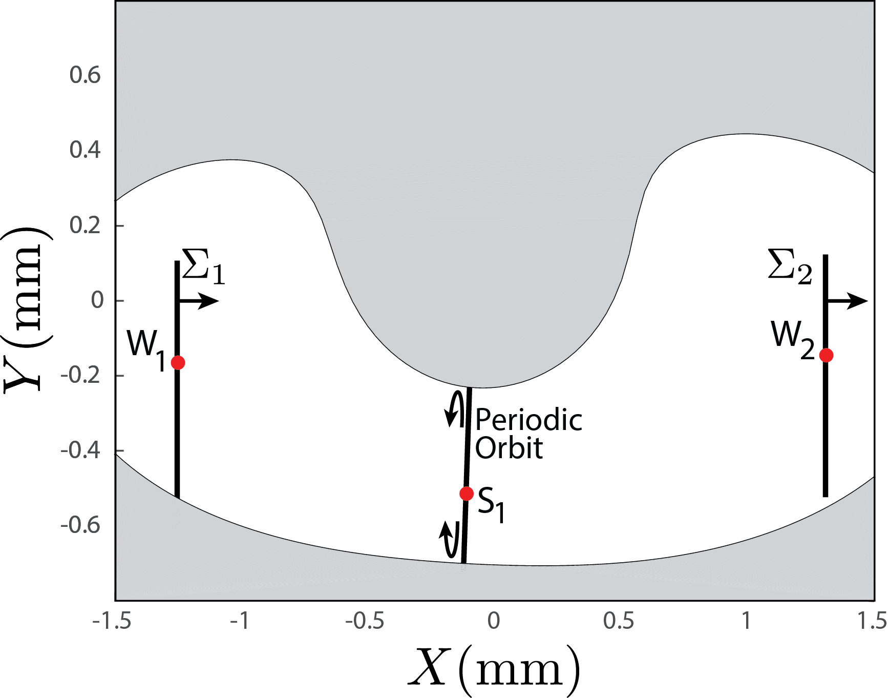
Figure 7: For a representative energy above the saddle point S₁, we show the unstable periodic orbit in the neck region around S₁. It projects to a single line going between the upper and lower energy boundary curves, and arrows are shown for convenience. We show the Poincaré sections $\Sigma_{1}$ and $\Sigma_{2}$ which are defined by $X$ values equal to that of the two stable equilibria in the center of the left and right side wells, W₁ and W₂, respectively. The arrows on the vertical lines indicate that these Poincaré sections are also defined by positive $X$ momentum.

Step 2: Compute the approximate transition tube and its intersection on a Poincaré section. We have analyzed the flow of linearized system in both phase space and position space which classifies orbits into four classes. It shows that in the conservative system the stable manifolds correspond to the boundary between transit orbits and non-transit orbits. Thus, we can choose this manifold as the starting point. We start by considering the approximation of transition tubes for the conservative system.

Determine the initial condition. The stable manifold divides the transit orbits and non-transit orbits for all trajectories headed toward a bottleneck. Thus, we can use the stable manifold to obtain the initial condition. Considering the general solutions (56) of the linearized equations (36), we can let $p_{1}^{0}=c$, $q_{1}^{0}=0$, $q_{2}^{0}=A_{q}$ and $p_{2}^{0}=A_{p}$. Notice that

$$A_{q}^{2}+A_{p}^{2}=2h/\omega_{p}$$ (87)

which forms a circle in the center projection, so in the next computational procedure we should pick up $N$ points on the circle with a constant arc length interval. Each $A_{q}$ and $A_{p}$ determined by these sampling points along with $p_{1}^{0}=c$ and $q_{1}^{0}=0$ can be used as initial conditions. When first transformed back to the position space and then transformed to dimensional quantities, this yields an initial condition

$$\begin{pmatrix}X_{0}\\ Y_{0}\\ p_{X0}\\ p_{Y0}\end{pmatrix}=\begin{pmatrix}x_{e}\\ y_{e}\\ 0\\ 0\end{pmatrix}+\begin{pmatrix}L_{x}\\ L_{y}\\ \omega_{0}L_{x}M_{1}\\ \omega_{0}L_{y}M_{2}\end{pmatrix}^{T}C\begin{pmatrix}c\\ 0\\ A_{q}\\ A_{p}\end{pmatrix}$$ (88)

Integrate backward and obtaining Poincaré section. Using the $N$ initial conditions (88) yielded by varying $A_{q}$ and $A_{p}$ governed by (87) and integrating the nonlinear equations of motions in (LABEL:eq:eomHam) in the backward direction, we obtain a tube, formed by the $N$ trajectories, which is a linear approximation for the transition tube. Choosing the Poincaré surface-of-section $\Sigma_{1}$ is shown in Figure 7, corresponding to $X=X_{{\rm W}_{1}}$ and $p_{X}>0$.

Step 3: Compute the real transition tube by the bisection method. We have obtained a Poincaré section which is the intersection of the approximate transition tube and the surface $\Sigma_{1}$. First pick a point (noted as $p_{i}$) which is almost the center of the closed curve. The line from $p_{i}$ to each of the $N$ points on the Poincaré map will form a ray. The point $p_{i}$ inside the curve in general is a transit orbit. Then choose another point on each radius which is a non-transit orbit, noted as $p_{o}$. With the approach described above, we can use the bisection method to obtain the boundary of the transition tube on a specific radius (cf. [25]). Picking the midpoint (marked by $p_{m}$) as the initial condition and carrying out forward integration for the nonlinear equation of motion in (LABEL:eq:eomHam), we can estimate if this trajectory can transit or not. If it is a transit orbit, note it as $p_{i}$, or note it as $p_{o}$. Continuing this procedure again until the distance between $p_{i}$ and $p_{o}$ reaches a specified tolerance, the boundary of the tube on this ray is estimated. Thus, the real transition tube for the conservative system can be obtained if the same procedure is carried out for all angles. A related method is described in [26], adapting an approach of [27].

For the dissipative system, the size of the transition tubes for a given energy on $\Sigma_{1}$ will shrink. Using the bisection method and following the same procedure as for conservative system, the transition tube for the dissipative system will be obtained.

5.2 Numerical results and discussion

To visualize the tube dynamics for the arch, several examples will be given. According to the steps mentioned above, we can obtain the transition tubes for both the conservative system and dissipative systems. For all results, the geometries of the arch are selected as $b=12.7$ mm $d=0.787$ mm, $L=228.6$ mm. The Young’s modulus and the mass density are $E=153.4$ GPa and $\rho=7567\ \mathrm{kg\ m^{-3}}$. The selected thermal load corresponds to $184.1$ N, while the initial imperfections are $\gamma_{1}=0.082$ mm and $\gamma_{2}=-0.077$ mm. These values match the parameters given in the experimental study [1]. For all the numerical results given in this section, the initial energy of the system is set at 3.68$\times 10^{-4}$ J - above the energy of saddle point S₁, so that the equilibrium point $W_{1}$ is inside the configuration space projection. This choice of initial energy will make it possible to compare the numerical results with the experimental results which are planned for future work.

Transition tubes for conservative system

For conservative system, the Hamiltonian is a constant of motion. In Figure 8, we show the configuration space projection of the transition tube and the Poincaré sections on $\Sigma_{1}$ and $\Sigma_{2}$ which are closed curves. In Figure 8 are shown all the trajectories which form the transition tube boundary starting from $\Sigma_{1}$ and ending up at $\Sigma_{2}$, flowing from left to right through the neck region.

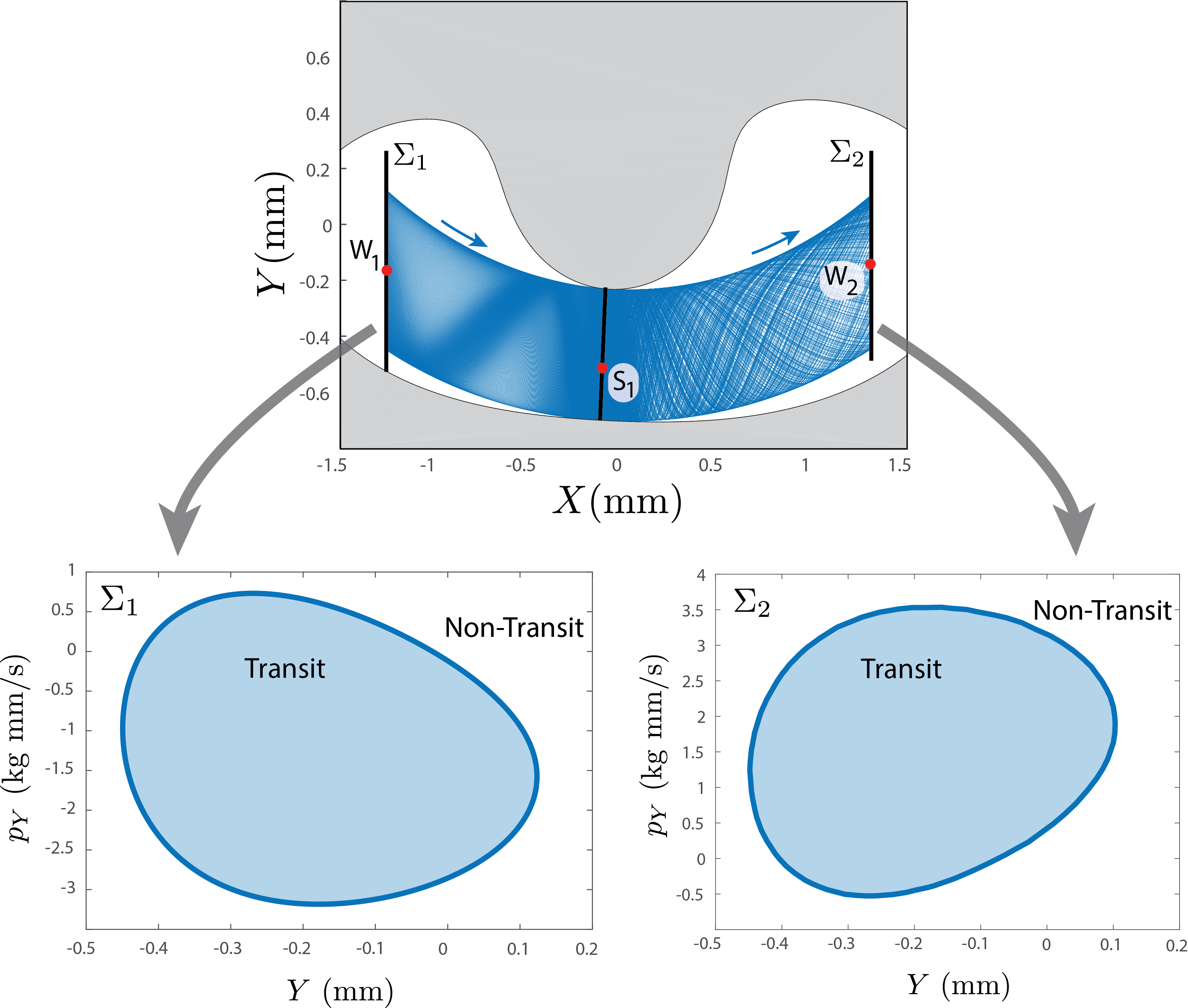
Figure 8: A transition tube from the left well to the right well, obtained using the method described in the text. The upper figure shows the configuration space projection. The lower left shows the tube boundary (closed curve) on Poincaré section $\Sigma_{1}$, which separates transit and non-transit trajectories. The lower right shows the corresponding tube boundary (closed curve) on Poincaré section $\Sigma_{2}$.

Due to the the conservation of energy, the size of the transition tube is constant during evolution, which corresponds to the cross-sectional area of the transition tube. It should be noted that the areas of the tube Poincaré sections on $\Sigma_{1}$ and $\Sigma_{2}$ in Figure 8 are equal, due to the integral invariants of Poincaré for a system obeying Hamilton’s canonical equations (with no damping). Moreover, note that the size of the transition tube, the boundary of the transit orbits, is determined by the energy. For a lower energy, the size of the transition tube is smaller or vice versa. In other words, the area of the Poincaré sections on $\Sigma_{1}$ and $\Sigma_{2}$ is determined by the energy. In fact, the cross-sectional area of the transition tube is proportional to the energy above the saddle point S₁ [28]. As mentioned before, the transition tube separates the transit orbits and non-transit orbits, which correspond to snap-through and non-snap-through. The orbit inside the transition tube can transit, while the orbit outside the transition tube cannot transit.

Transition tubes for dissipative system

Unlike the conservation of energy in conservative system, the energy in the dissipative system is decreasing with time.

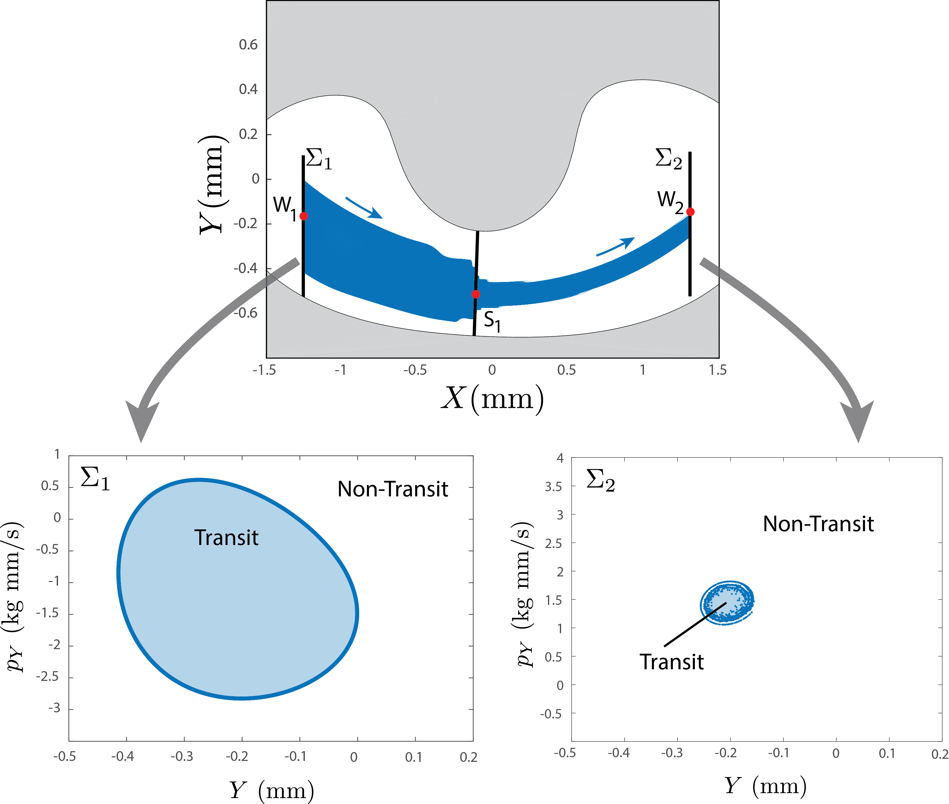
Figure 9: A transition tube from the left well to the right well, obtained using the method described in the text, for the case of damping. The upper figure shows the configuration space projection. The lower left shows the tube boundary (closed curve) on Poincaré section $\Sigma_{1}$ which separates transit and non-transit trajectories for initial conditions all with a given fixed initial energy. The lower right shows the corresponding image under the flow on Poincaré section $\Sigma_{2}$. Due to the damping, and a range of times spent in the neck region, spiraling is visible in this 2D projection since trajectories which spend longer in the neck will be at lower total energies. Compare with Figure 8.

Figure 9 shows the configuration space projection of the transition tube and the Poincaré sections on $\Sigma_{1}$ and $\Sigma_{2}$. In Figure 9 the transition tube starts from $\Sigma_{1}$ and ends up with $\Sigma_{2}$ flowing from left to right through the neck region, as shown previously for the conservative system. From the figure, we can observe the distinct reduction in the size of the transition tube, especially near the neck region. To show this, the scale of the Poincaré section projections is the same as in Figure 8. During the evolution, the energy of the system is decreasing due to damping. The trajectories spend a great amount of time crossing the neck region, resulting in the total energy decreasing dramatically (and influencing the size of the transition tubes to the right of the neck region). Thus, the transition tube is spiraling in the neck region so that Poincaré $\Sigma_{2}$ is not a closed curve, nor are the trajectories at a constant energy. The $\Sigma_{2}$ plot is merely a projection onto the $(Y,p_{Y})$-plane to give an idea of the actual co-dimension 1 tube boundary in the 4-dimensional phase space. Note the clear differences between Figure 8 and Figure 9. The dramatic shrinking of tubes near the neck region is due almost entirely to the linearized dynamics near the saddle point. To confirm this, we present the linear transition tube obtained by the analytical solutions (77) for the linearized dissipative system in Figure 10.

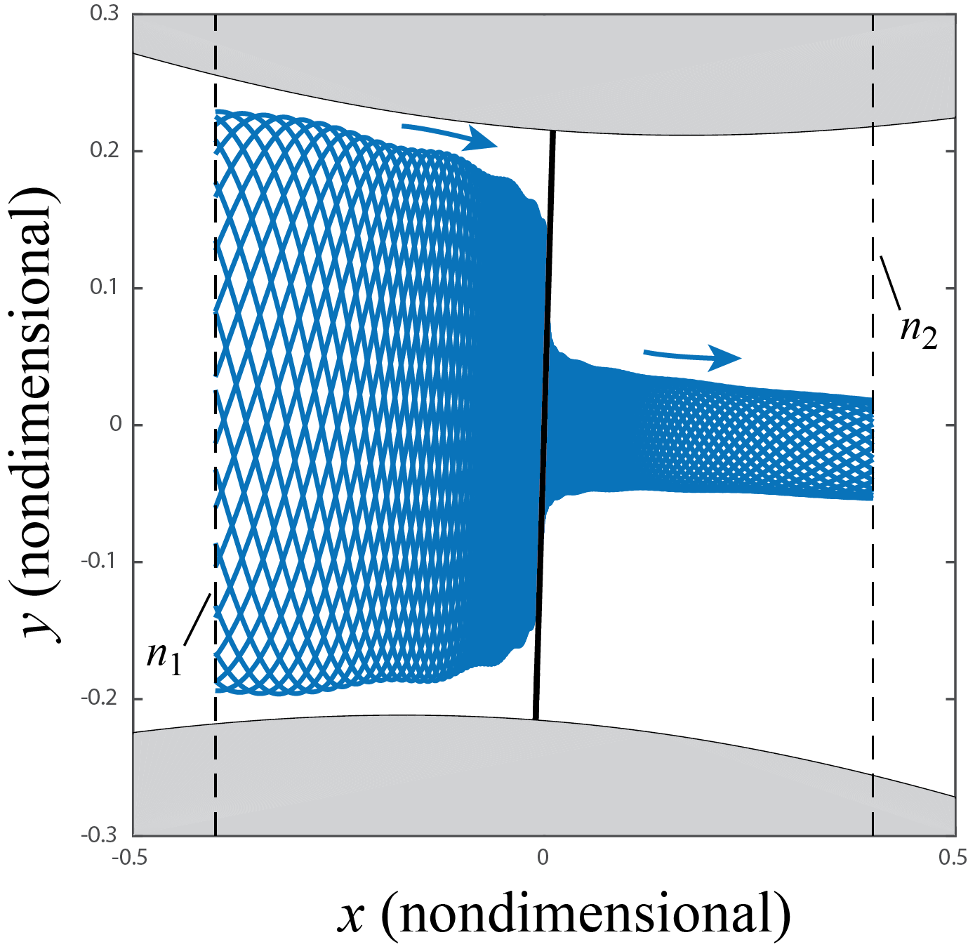
Figure 10: A transition tube from the left side boundary ($n_{1}$) to the right side boundary ($n_{2}$) of the equilibrium region around saddle point S₁, obtained for the linear damped system. Notice that the shrinking of the tube is observed as in the nonlinear system, Figure 9, here seen in terms of the width of the projected strip onto configuration space.

Effect of damping on the transition tubes

In order to further quantify how damping affects the size of transition tubes, we present the tube Poincaré section on $\Sigma_{1}$ with different damping in Figure 11. In Figure 11(a), we can see the canonical area ($\int_{\mathcal{A}}p_{Y}dY$) decreases with increasing damping. Thus, the proportion of transition trajectories will be fewer if the damping increases. Note that when the damping changes, different transition tubes almost share the same center which corresponds to the fastest trajectories. Figure 11(b) shows the relation between the damping and the projected canonical area ($\int_{\mathcal{A}}p_{Y}dY$), which is related to the relative number of transit compared to non-transit orbits. It shows that an increase in damping decreases the projected area. When the damping is small, the relation between the damping and the area is linear, while when the damping is large, the relation becomes slightly nonlinear. Note that generally in mechanical/structural experiments the non-dimensional damping factor $\xi_{d}$ is less than $5\%$ which corresponds to a damping coefficient $C_{H}$ less than $107.3\ \mathrm{s^{-1}}$ (see the shaded region in Figure 11(b)). Furthermore, note that for the initial energy depicted in Figure 11, there are are no transit orbits starting on $\Sigma_{1}$ for $C_{H}$ greater than about $185\ \mathrm{s^{-1}}$.

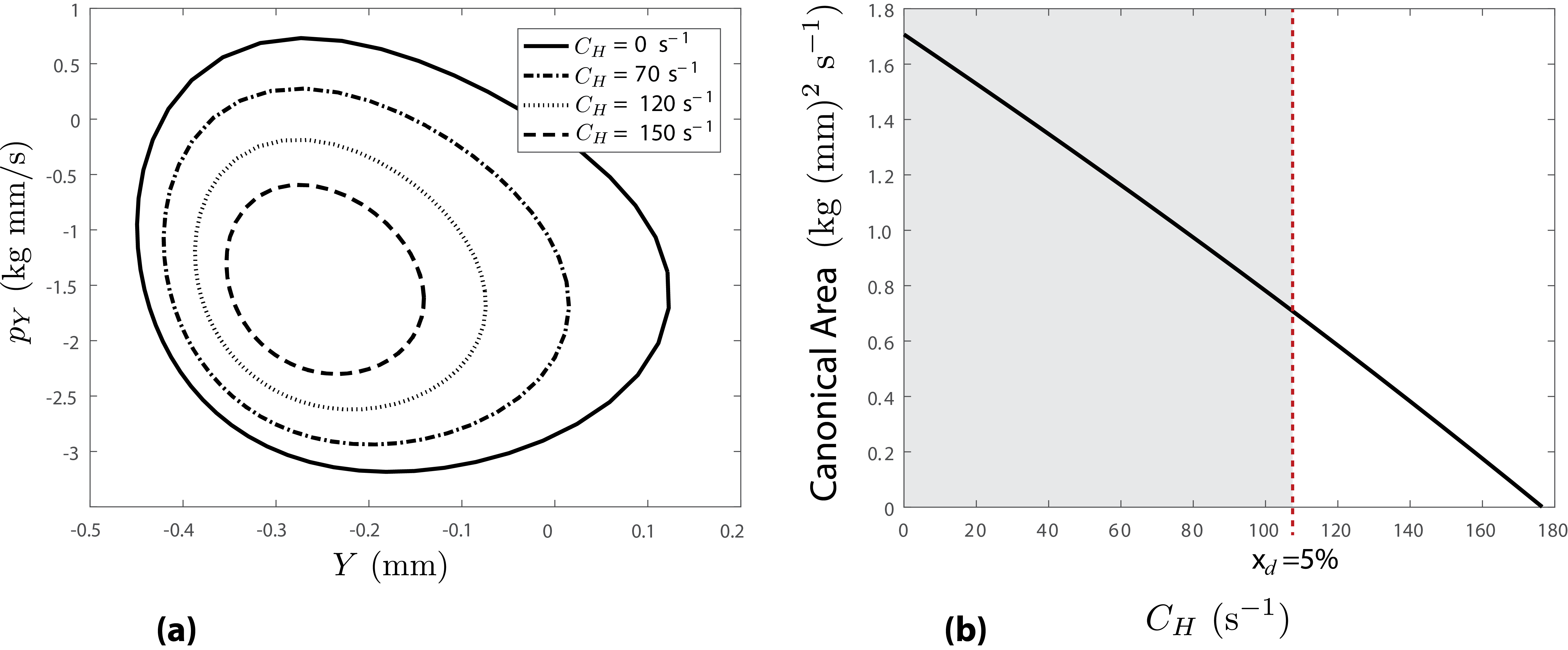
Figure 11: The effect of the damping coefficient $C_{H}$ on the area of the transition tube on Poincaré section $\Sigma_{1}$ is shown. For a fixed initial energy above the saddle, the projection on the canonical plane $(Y,p_{Y})$ is shown in (a) and the area is plotted in (b). In (b), the shaded region indicates the experimentally observed range of damping coefficients, which correspond to non-dimensional damping factor $\xi_{d}$ less than 5%.

Demonstration of trajectories inside and outside the transition tube

To illustrate the effectiveness of the transition tubes, we choose three points on $\Sigma_{1}$ (see A, B and C in Figure 12(a)) as the initial conditions and integrate forward to see their evolution.

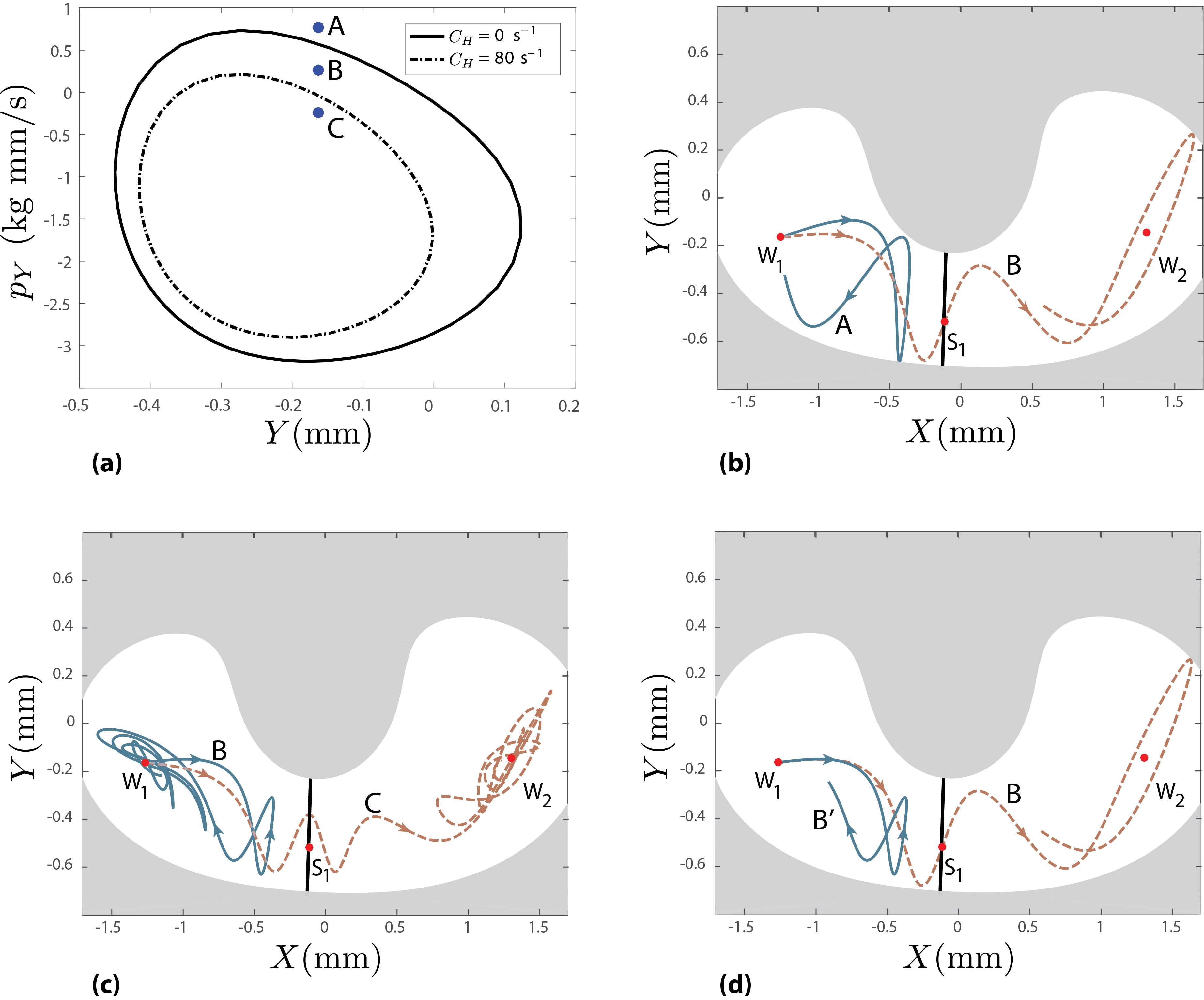
Figure 12: Several example trajectories are shown, starting from the stable well point W₁. The initial conditions from Poincaré section $\Sigma_{1}$ are shown in (a) for a fixed initial energy, along with the transition tube boundaries for the conservative case and a damped case. In (b), we show the trajectories for points A and B, for the conservative case where A is just outside the tube boundary and B is just inside. In (c), we show the trajectories for points B and C, for the damped case where B is just outside the tube boundary and C is just inside. In (d), we illustrate the effect of damping by starting the same initial condition, B, but showing the trajectory in the conservative case as trajectory B and the damped case as trajectory B^′.

Note that all the trajectories corresponding to these three points have the same initial energy and start from a configuration identical to the equilibrium point $W_{1}$, but with different initial velocity directions. Figure 12(b) shows the trajectories A and B in the conservative system where A is outside the tube boundary and B is inside the tube boundary. In the figure, trajectory B transits through the neck region and trajectory A bounces back. Figure 12(c) shows trajectories B and C in the dissipative system. Like the situation in the conservative system, trajectory C which is inside the tube can transit, while trajectory B which is outside the tube cannot. Figure 12(d) shows the effect of damping on the transit condition for the trajectories B and B^′ with the same initial condition. Trajectory B is simulated using the conservative system and trajectory B^′ is simulated using the dissipative system. It shows that the damping changes the transit condition that a transit orbit B in the conservative system becomes non-transit orbit B^′ in the dissipative system, both starting from the same initial condition. From Figure 12, we can conclude the transition tube can effectively estimate the snap-through transitions both in conservative systems and dissipative systems.

Finally, we point out that the transition tubes are the boundary for transit orbits that transition the first time. For example, trajectory A in Figure 12(b) stays outside of the transition tube so that it returns near the neck region at first, but, unless it happens to be on a KAM torus or a stable manifold of such a torus, it will ultimately transit as long as it does not form a periodic orbit near the potential well W₁, since the energy is above the critical energy for transition and is conservative.

6 Conclusions

Tube dynamics is a conceptual dynamical systems framework initially used to study the isomerization reactions in chemistry [12, 13, 14, 15, 29] as well as other fields, like resonance transitions in celestial mechanics [11, 9, 30, 17, 18] and capsize in ship dynamics [8]. Here we extend the application of tube dynamics to structural mechanics: the snap-through of a shallow arch, or buckled-beam. In general, slender elastic structures are capable of exhibiting a variety of (co-existing) equilibrium shapes, and thus, given a disturbance, tube dynamics sheds light on how such a system might be caused to transition between available, stable equilibrium configurations. Moreover, it is the first time, to the best of our knowledge, that tube dynamics has been worked out for a dissipative system, which increases the generality of the approach.

The snap-through transition of an arch was studied via a two-mode truncation of the governing partial differential equations based on Euler-Bernoulli beam theory. Via analysis of the linearized Hamiltonian equations around the saddle, the analytical solutions for both the conservative and dissipative systems were determined and the corresponding flows in the equilibrium region of eigenspace and configuration space were discussed. The results show that all transit orbits, corresponding to snap-through, must evolve from a wedge of velocities which are restricted to a strip in configuration space in the conservative system, and by an ellipse in the corresponding dissipative system when damping is included. Using the results from the linearization as an approximation, the transition tubes based on the full nonlinear equations for both the conservative and dissipative system were obtained by the bisection method. The orbits inside the transition tubes can transit, while the orbits outside the tubes cannot. Results also show that the damping makes the size of the transition tubes smaller, which corresponds to the degree, or amount, of orbits that transit. When the damping is small, it has a nearly linear effect on the size of the transition tubes.

Further study of the dynamic behaviors of the arch can lead to more immediate application structural mechanics. For example, many structural systems possess multiple equilibria, and the manner in which the governing potential energy changes with a control parameter is, of course, the essence of bifurcation theory. However, under nominally fixed conditions, the present paper directly assesses the energy required to (dynamically) perturb a structural system beyond the confines of its immediate potential energy well. In future work, a three-mode truncation may be introduced to study such systems. High order approximations will present higher index saddles which will modify the tube dynamics framework presented here (cf. [31] [32] [33]). Furthermore, experiments will be carried out to show the effectiveness of the present approach to prescribe initial conditions which lead to dynamic buckling.

7 Acknowledgements

This work was supported in part by the National Science Foundation under awards 1150456 (to SDR) and 1537349 (to SDR and LNV). One of the authors (SDR) acknowledges enjoyable interactions during the past decade with Professor Romesh Batra, who is being honored by this issue.

References

- [1] Wiebe, R. and Virgin, L. N. [2016] On the experimental identification of unstable static equilibria. Proceedings of the Royal Society of London A: Mathematical, Physical and Engineering Sciences 472(2190):20160172.
- [2] Collins, P., Ezra, G. S. and Wiggins, S. [2012] Isomerization dynamics of a buckled nanobeam. Physical Review E 86(5):056218.
- [3] Virgin, L., Guan, Y. and Plaut, R. [2017] On the geometric conditions for multiple stable equilibria in clamped arches. International Journal of Non-Linear Mechanics 92:8–14.
- [4] Das, K. and Batra, R. [2009] Symmetry breaking, snap-through and pull-in instabilities under dynamic loading of microelectromechanical shallow arches. Smart Materials and Structures 18(11):115008.
- [5] Das, K. and Batra, R. [2009] Pull-in and snap-through instabilities in transient deformations of microelectromechanical systems. Journal of Micromechanics and Microengineering 19(3):035008.
- [6] Mann, B. [2009] Energy criterion for potential well escapes in a bistable magnetic pendulum. Journal of Sound and Vibration 323(3):864–876.
- [7] Thompson, J. M. T. and Hunt, G. W. [1984] Elastic Instability Phenomena. Wiley.
- [8] Naik, S. and Ross, S. D. [2017] Geometry of escaping dynamics in nonlinear ship motion. Communications in Nonlinear Science and Numerical Simulation 47:48 – 70.
- [9] Koon, W. S., Lo, M. W., Marsden, J. E. and Ross, S. D. [2000] Heteroclinic connections between periodic orbits and resonance transitions in celestial mechanics. Chaos 10:427–469.
- [10] Conley, C. C. [1968] Low energy transit orbits in the restricted three-body problem. SIAM J. Appl. Math. 16:732–746.
- [11] Llibre, J., Martinez, R. and Simó, C. [1985] Transversality of the invariant manifolds associated to the Lyapunov family of periodic orbits near L2 in the restricted three-body problem. J. Diff. Eqns. 58:104–156.
- [12] Ozorio de Almeida, A. M., De Leon, N., Mehta, M. A. and Marston, C. C. [1990] Geometry and dynamics of stable and unstable cylinders in Hamiltonian systems. Physica D 46:265–285.
- [13] De Leon, N., Mehta, M. A. and Topper, R. Q. [1991] Cylindrical manifolds in phase space as mediators of chemical reaction dynamics and kinetics. I. Theory. J. Chem. Phys. 94:8310–8328.
- [14] De Leon, N. [1992] Cylindrical manifolds and reactive island kinetic theory in the time domain. J. Chem. Phys. 96:285–297.
- [15] Topper, R. Q. [1997] Visualizing molecular phase space: nonstatistical effects in reaction dynamics. In Reviews in Computational Chemistry (edited by K. B. Lipkowitz and D. B. Boyd), vol. 10, chap. 3, 101–176. VCH Publishers, New York.
- [16] Gabern, F., Koon, W. S., Marsden, J. E. and Ross, S. D. [2005] Theory and Computation of Non-RRKM Lifetime Distributions and Rates in Chemical Systems with Three or More Degrees of Freedom. Physica D 211:391–406.
- [17] Gabern, F., Koon, W. S., Marsden, J. E., Ross, S. D. and Yanao, T. [2006] Application of tube dynamics to non-statistical reaction processes. Few-Body Systems 38:167–172.
- [18] Marsden, J. E. and Ross, S. D. [2006] New methods in celestial mechanics and mission design. Bulletin of the American Mathematical Society 43:43–73.
- [19] Koon, W. S., Lo, M. W., Marsden, J. E. and Ross, S. D. [2011] Dynamical Systems, the Three-Body Problem and Space Mission Design. Marsden Books, ISBN 978-0-615-24095-4.
- [20] Murphy, K. D., Virgin, L. N. and Rizzi, S. A. [1996] Experimental snap-through boundaries for acoustically excited, thermally buckled plates. Experimental Mechanics 36:312–317.
- [21] Wiebe, R., Virgin, L. N., Stanciulescu, I., Spottswood, S. M. and Eason, T. G. Characterizing Dynamic Transitions Associated with Snap-Through: A Discrete System. Journal of Computational and Nonlinear Dynamics 8.
- [22] Zhong, J., Fu, Y., Chen, Y. and Li, Y. [2016] Analysis of nonlinear dynamic responses for functionally graded beams resting on tensionless elastic foundation under thermal shock. Composite Structures 142:272–277.
- [23] Greenwood, D. T. [2003] Advanced Dynamics. Cambridge University Press.
- [24] Wiggins, S. [1994] Normally Hyperbolic Invariant Manifolds in Dynamical Systems. Springer-Verlag, New York.
- [25] Anderson, R. L., Easton, R. W. and Lo, M. W. [2017] Isolating blocks as computational tools in the circular restricted three-body problem. Physica D: Nonlinear Phenomena 343:38 – 50.
- [26] Onozaki, K., Yoshimura, H. and Ross, S. D. [2017] Tube dynamics and low energy Earth-Moon transfers in the 4-body system. Advances in Space Research ( ):to appear.
- [27] Gawlik, E. S., Marsden, J. E., Du Toit, P. C. and Campagnola, S. [2009] Lagrangian coherent structures in the planar elliptic restricted three-body problem. Celestial Mechanics and Dynamical Astronomy 103:227–249. doi:10.1007/s10569-008-9180-3.
- [28] MacKay, R. S. [1990] Flux over a saddle. Physics Letters A 145:425–427.
- [29] Jaffé, C., Farrelly, D. and Uzer, T. [1999] Transition state in atomic physics. Phys. Rev. A 60:3833–3850.
- [30] Jaffé, C., Ross, S. D., Lo, M. W., Marsden, J. E., Farrelly, D. and Uzer, T. [2002] Theory of asteroid escape rates. Physical Review Letters 89:011101.
- [31] Collins, P., Ezra, G. S. and Wiggins, S. [2011] Index k saddles and dividing surfaces in phase space with applications to isomerization dynamics. The Journal of chemical physics 134(24):244105.
- [32] Haller, G., Uzer, T., Palacian, J., Yanguas, P. and Jaffe, C. [2011] Transition state geometry near higher-rank saddles in phase space. Nonlinearity 24(2):527.
- [33] Nagahata, Y., Teramoto, H., Li, C.-B., Kawai, S. and Komatsuzaki, T. [2013] Reactivity boundaries for chemical reactions associated with higher-index and multiple saddles. Phys. Rev. E 88:042923.