Probing spinon nodal structures in three-dimensional Kitaev spin liquids

Abstract

We propose that resonant inelastic X-ray scattering (RIXS) is an effective probe of the fractionalized excitations in three-dimensional (3D) Kitaev spin liquids. While the non-spin-conserving RIXS responses are dominated by the gauge-flux excitations and reproduce the inelastic-neutron-scattering response, the spin-conserving (SC) RIXS response picks up the Majorana-fermion excitations and detects whether they are gapless at Weyl points, nodal lines, or Fermi surfaces. As a signature of symmetry fractionalization, the SC RIXS response is suppressed around the $\Gamma$ point. On a technical level, we calculate the exact SC RIXS responses of the Kitaev models on the hyperhoneycomb, stripyhoneycomb, hyperhexagon, and hyperoctagon lattices, arguing that our main results also apply to generic 3D Kitaev spin liquids beyond these exactly solvable models.

Quantum spin liquids (QSLs) are exotic and entirely quantum phases of matter Balents-2010 ; Savary-2016 hosting a remarkable set of emergent phenomena, including long-range entanglement, topological ground-state degeneracy, and fractionalized anyonic excitations. The Kitaev spin liquid (KSL) on the honeycomb lattice Kitaev-2006 and its generalizations on tricoordinated three-dimensional (3D) lattices Mandal-2009 ; Hermanns-2014 ; Hermanns-2015 ; O'Brien-2016 ; Hermanns-2017 are quintessential examples of such QSL phases. Importantly, recent years have seen much progress in identifying a large number of candidate materials for realizing these KSL phases Jackeli-2009 ; Chaloupka-2010 ; Chaloupka-2013 ; Trebst-2017 , such as the honeycomb iridates Na₂IrO₃ Singh-2010 ; Liu-2011 ; Singh-2012 ; Choi-2012 ; Ye-2012 ; Comin-2012 and $\alpha$-Li₂IrO₃ Williams-2016 , the honeycomb ruthenium chloride $\alpha$-RuCl₃ Plumb-2014 ; Sandilands-2015 ; Sears-2015 ; Majumder-2015 ; Johnson-2015 ; Sandilands-2016 ; Banerjee-2016 , and the 3D harmonic-honeycomb iridates $\beta$- and $\gamma$-Li₂IrO₃ Modic-2014 ; Biffin-2014a ; Biffin-2014b ; Takayama-2015 .

From a theoretical point of view, KSLs are particularly appealing because each of them has an exactly solvable limit governed by a Kitaev model Kitaev-2006 . In general, the Kitaev model is defined on a tricoordinated lattice with $S=1/2$ spins $\sigma_{\mathbf{r}}^{x,y,z}$ at the sites $\mathbf{r}$, which are coupled to their neighbors via bond-dependent Ising interactions. The Hamiltonian reads

$$H=-J_{x}\sum_{\langle\mathbf{r},\mathbf{r}^{\prime}\rangle_{x}}\sigma_{\mathbf{r}}^{x}\sigma_{\mathbf{r}^{\prime}}^{x}-J_{y}\sum_{\langle\mathbf{r},\mathbf{r}^{\prime}\rangle_{y}}\sigma_{\mathbf{r}}^{y}\sigma_{\mathbf{r}^{\prime}}^{y}-J_{z}\sum_{\langle\mathbf{r},\mathbf{r}^{\prime}\rangle_{z}}\sigma_{\mathbf{r}}^{z}\sigma_{\mathbf{r}^{\prime}}^{z},$$ (1)

where $J_{x,y,z}$ are the coupling constants for the three types of bonds $x$, $y$, and $z$. Remarkably, this model is exactly solvable whenever there is precisely one bond of each type around each site of the tricoordinated lattice.

These exactly solvable Kitaev models have been defined on a wide range of tricoordinated 3D lattices Mandal-2009 ; Hermanns-2014 ; Hermanns-2015 ; O'Brien-2016 ; Hermanns-2017 , including the hyperhoneycomb, stripyhoneycomb, hyperhexagon, and hyperoctagon lattices (see Fig. 1). In the experimentally relevant isotropic regime ($J_{x}\approx J_{y}\approx J_{z}$), the ground state is a gapless $\mathbb{Z}_{2}$ QSL, while the (fractionalized) excitations are gapless Majorana fermions and gapped $\mathbb{Z}_{2}$ gauge fluxes. Importantly, the Majorana fermions (spinons) exhibit a rich variety of nodal structures due to the different (projective) ways symmetries can act on them Hermanns-2014 ; Hermanns-2015 ; O'Brien-2016 . Indeed, they are gapless along nodal lines for the hyperhoneycomb and the stripyhoneycomb models Mandal-2009 , on Fermi surfaces for the hyperoctagon model Hermanns-2014 , and at Weyl points for the hyperhexagon model O'Brien-2016 .

From an experimental point of view, however, it is difficult to identify and characterize QSLs due to the lack of any local order parameters that could be used as ”smoking-gun” signatures. In recent years, a remarkable theoretical and experimental progress has been achieved in understanding that fractionalization is one of the most promising hallmarks of a QSL. Indeed, it has been demonstrated that fractionalized excitations, which are Majorana fermions and $\mathbb{Z}_{2}$ gauge fluxes for KSLs, can be probed by conventional spectroscopic techniques, such as inelastic neutron scattering (INS) Banerjee-2016 ; Knolle-2014a ; Knolle-2015 ; Smith-2015 ; Smith-2016 , Raman scattering with visible light Sandilands-2015 ; Sandilands-2016 ; Knolle-2014b ; Perreault-2015 ; Perreault-2016a ; Perreault-2016b ; Glamazda-2016 , and resonant inelastic X-ray scattering (RIXS) Ko-2011 ; Savary-2015 ; Halasz-2016 .

In this Letter, we propose that RIXS is an effective probe of the spinon (semi)metals realized in 3D KSLs. Calculating the exact RIXS responses of four different 3D Kitaev models (see lattices in Fig. 1), we demonstrate that nodal lines, Weyl points, and Fermi surfaces of Majorana fermions leave distinct characteristic fingerprints in the spin-conserving (SC) RIXS response. For the hyperhoneycomb and the stripyhoneycomb models, corresponding to $\beta$- and $\gamma$-Li₂IrO₃, the SC RIXS response is gapless within particular high-symmetry planes but not at a generic point of the Brillouin zone. In contrast, for the hyperhexagon model, it is gapless at particular points only, while for the hyperoctagon model, it is gapless in almost the entire Brillouin zone. Also, the SC RIXS response is found to be strongly suppressed around the $\Gamma$ point for all four models as a result of symmetries acting projectively on the Majorana fermions. We argue that our results apply to generic KSLs and not only to the pure Kitaev models.

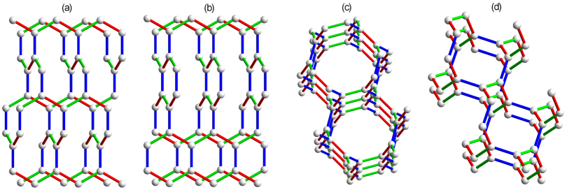
Figure 1: Tricoordinated 3D lattices of the Kitaev models considered in this work: (a) hyperhoneycomb, (b) stripyhoneycomb, (c) hyperhexagon, and (d) hyperoctagon lattices. Different bond types $x$, $y$, and $z$ are marked by red, green, and blue, respectively.

General RIXS formalism.—Motivated by the available candidate materials ($\beta$- and $\gamma$-Li₂IrO₃), we calculate the RIXS responses for the $L_{3}$ edge of the Ir⁴⁺ ion which is in the $5d^{5}$ configuration Ament-2011a ; Kim-2017 . However, our results are also expected to be valid for other RIXS edges and for other potential $d^{5}$ candidate materials Halasz-2016 . During RIXS, an incoming photon is absorbed and excites a $2p$ core electron into the $5d$ valence shell, which then decays back into the $2p$ core hole and emits an outgoing photon Ament-2011b . The low-energy physics of the $5d$ valence shell at each Ir⁴⁺ ion is governed by a $J=1/2$ Kramers doublet in the $t_{2g}$ orbitals, and we assume that the low-energy Hamiltonian acting on these Kramers doublets is the Kitaev Hamiltonian in Eq. (1). In terms of the corresponding Kitaev model, the $5d^{6}$ configuration in the intermediate state is then described as a non-magnetic vacancy Willans-2010 ; Willans-2011 ; Halasz-2014 ; Sreejith-2016 .

The initial and the final states of RIXS are $|0\rangle\otimes|\mathbf{Q},\bm{\epsilon}\rangle$ and $|m\rangle\otimes|\mathbf{Q}^{\prime},\bm{\epsilon}^{\prime}\rangle$, respectively, where $|0\rangle$ is the ground state of the Kitaev model, $|m\rangle$ is a generic eigenstate with energy $E_{m}$ with respect to $|0\rangle$, while $\mathbf{Q}$ ($\mathbf{Q}^{\prime}$) is the momentum and $\bm{\epsilon}$ ($\bm{\epsilon}^{\prime}$) is the polarization of the incoming (outgoing) photon. During RIXS, an energy $\omega=c\,\{|\mathbf{Q}|-|\mathbf{Q}^{\prime}|\}=E_{m}$ and a momentum $\mathbf{q}=\mathbf{Q}-\mathbf{Q}^{\prime}$ is transferred from the scattered photon to the KSL. Summing over all final states $|m\rangle$, the total RIXS intensity is then $I(\omega,\mathbf{q})=\sum_{m}|A(m,\mathbf{q})|^{2}\,\delta(\omega-E_{m})$, where $A(m,\mathbf{q})$ are the individual RIXS amplitudes.

Since RIXS has four fundamental channels Halasz-2016 , each RIXS amplitude takes the form $A(m,\mathbf{q})=\sum_{\eta}P_{\eta}A_{\eta}(m,\mathbf{q})$, where $P_{\eta}$ are polarization factors depending on $\bm{\epsilon}$ and $\bm{\epsilon}^{\prime}$ Ament-2011a , while $A_{\eta}(m,\mathbf{q})$ are single-channel RIXS amplitudes corresponding to the four fundamental channels. In the SC channel labeled by $\eta=0$, the spin of the $5d$ valence shell does not change during RIXS, while in the three non-spin-conserving (NSC) channels labeled by $\eta=x,y,z$, the same spin is rotated by $\pi$ around the $x,y,z$ axes, respectively.

The single-channel RIXS amplitudes $A_{\eta}(m,\mathbf{q})$ are given by the Kramers$-$Heisenberg formula Ament-2011b . In the experimentally relevant fast-collision regime, where the core-hole decay rate $\Gamma$ is much larger than the Kitaev coupling constants $J_{x,y,z}$ (e.g., for the iridates: $\Gamma/J_{x,y,z}\sim 100$) Clancy-2012 ; Katukuri-2014 , these RIXS amplitudes take the lowest-order form Halasz-2016

$$A_{\eta}(m,\mathbf{q}) \propto \sum_{\mathbf{r}}e^{i\mathbf{q}\cdot\mathbf{r}}\langle m|\sigma_{\mathbf{r}}^{\eta}\bigg{[}1-\frac{i\tilde{H}(\mathbf{r})}{\Gamma}\bigg{]}|0\rangle$$

$$= \sum_{\mathbf{r}}e^{i\mathbf{q}\cdot\mathbf{r}}\langle m|\sigma_{\mathbf{r}}^{\eta}\bigg{[}1-\frac{i}{\Gamma}\sum_{\kappa=x,y,z}J_{\kappa}^{\phantom{\kappa}}\sigma_{\mathbf{r}}^{\kappa}\sigma_{\kappa(\mathbf{r})}^{\kappa}\bigg{]}|0\rangle,$$

where $\tilde{H}(\mathbf{r})=H+\sum_{\kappa}J_{\kappa}^{\phantom{\kappa}}\sigma_{\mathbf{r}}^{\kappa}\sigma_{\kappa(\mathbf{r})}^{\kappa}$ is the Hamiltonian of the Kitaev model with a single vacancy at site $\mathbf{r}$. The spin at site $\mathbf{r}$ is effectively removed from the model by being decoupled from its neighbors at sites $\kappa(\mathbf{r})$ Halasz-2014 . Note also that $\sigma_{\mathbf{r}}^{0}$ is the identity operator and that we demand $H|0\rangle=0$ by adding a trivial constant term to $H$ in Eq. (1).

For the NSC channels, the RIXS amplitudes in Eq. (Probing spinon nodal structures in three-dimensional Kitaev spin liquids) reduce to spin-polarized INS amplitudes $\sum_{\mathbf{r}}e^{i\mathbf{q}\cdot\mathbf{r}}\langle m|\sigma_{\mathbf{r}}^{x,y,z}|0\rangle$ in the limit of $\Gamma\rightarrow\infty$. In the physically relevant regime, the three NSC RIXS responses thus reproduce the respective components of the dynamical spin structure factor studied in Refs. Smith-2015 and Smith-2016 . Indeed, since the NSC channels involve flux creation, the corresponding responses exhibit an overall flux gap and little momentum dispersion Halasz-2016 .

For the SC channel, however, taking the limit of $\Gamma\rightarrow\infty$ in Eq. (Probing spinon nodal structures in three-dimensional Kitaev spin liquids) gives a trivial amplitude $\sum_{\mathbf{r}}e^{i\mathbf{q}\cdot\mathbf{r}}\langle m|0\rangle$ that corresponds to a purely elastic process. The lowest-order inelastic process is then captured by the second term in Eq. (Probing spinon nodal structures in three-dimensional Kitaev spin liquids), and the corresponding RIXS amplitude can be calculated via the exact solution of the Kitaev model Kitaev-2006 . Furthermore, since the SC channel creates no fluxes, the entire calculation is restricted to the ground-state flux sector of the model.

Spinon band structures.—As a first step of our calculation, we describe the fermion (spinon) band structures of the four Kitaev models. Using the Kitaev fermionization $\sigma_{\mathbf{r}}^{\kappa}=ib_{\mathbf{r}}^{\kappa}c_{\mathbf{r}}^{\phantom{\kappa}}$ with $\kappa=x,y,z$, the Hamiltonian in Eq. (1) becomes

$$H=\sum_{\kappa}\sum_{\langle\mathbf{r},\mathbf{r}^{\prime}\rangle_{\kappa}}iJ_{\kappa}^{\phantom{\kappa}}u_{\mathbf{r},\mathbf{r}^{\prime}}^{\kappa}c_{\mathbf{r}}^{\phantom{\kappa}}c_{\mathbf{r}^{\prime}}^{\phantom{\kappa}}=\frac{1}{2}\sum_{\mathbf{r},\mathbf{r}^{\prime}}\mathcal{H}_{\mathbf{r},\mathbf{r}^{\prime}}c_{\mathbf{r}}c_{\mathbf{r}^{\prime}},$$ (3)

where $u_{\mathbf{r},\mathbf{r}^{\prime}}^{\kappa}\equiv ib_{\mathbf{r}}^{\kappa}b_{\mathbf{r}^{\prime}}^{\kappa}=\pm 1$ in the ground-state flux sector, while $\mathcal{H}_{\mathbf{r},\mathbf{r}^{\prime}}=iJ_{\kappa}^{\phantom{\kappa}}u_{\mathbf{r},\mathbf{r}^{\prime}}^{\kappa}$ if $\mathbf{r}$ and $\mathbf{r}^{\prime}$ are neighboring sites connected by a $\kappa$ bond and $\mathcal{H}_{\mathbf{r},\mathbf{r}^{\prime}}=0$ otherwise. It is known that the ground state of the hyperhexagon model has a $\pi$ flux at each elementary loop O'Brien-2016 ; Lieb-1994 , while we assume that the ground states of the remaining three models are flux free. This choice is consistent with numerical results for the hyperhoneycomb and the hyperoctagon models Mandal-2009 ; O'Brien-2016 , while it is merely a simplification for the stripyhoneycomb model Footnote-1 .

The quadratic fermion Hamiltonian in Eq. (3) can be diagonalized via a standard procedure. Since the lattice of each Kitaev model has $n$ sites per unit cell ($\nu=1,2,\ldots,n$), the resulting band structure has $n$ fermion bands ($\mu=1,2,\ldots,n$), where $n=4$ for the hyperhoneycomb and the hyperoctagon models, $n=6$ for the hyperhexagon model, and $n=8$ for the stripyhoneycomb model. For a lattice of $N$ unit cells, the fermion with band index $\mu$ and momentum $\mathbf{k}$ takes the form

$$\psi_{\mathbf{k},\mu}^{{\dagger}}=\frac{1}{\sqrt{2N}}\sum_{\nu=1}^{n}\big{(}\mathcal{W}_{\mathbf{k}}^{\phantom{{\dagger}}}\big{)}_{\nu\mu}\sum_{\mathbf{r}\in\nu}c_{\mathbf{r}}^{\phantom{{\dagger}}}\,e^{i\mathbf{k}\cdot\mathbf{r}},$$ (4)

while the corresponding fermion energy is $\varepsilon_{\mathbf{k},\mu}=2(\mathcal{E}_{\mathbf{k}})_{\mu\mu}$, where $\hat{\mathcal{H}}_{\mathbf{k}}^{\phantom{{\dagger}}}=\mathcal{W}_{\mathbf{k}}^{\phantom{{\dagger}}}\cdot\mathcal{E}_{\mathbf{k}}^{\phantom{{\dagger}}}\cdot\mathcal{W}_{\mathbf{k}}^{{\dagger}}$ is the (unitary) eigendecomposition of the Hermitian matrix $\hat{\mathcal{H}}_{\mathbf{k}}^{\phantom{{\dagger}}}$ with elements

$$(\hat{\mathcal{H}}_{\mathbf{k}})_{\nu\nu^{\prime}}=\frac{1}{N}\sum_{\mathbf{r}\in\nu}\sum_{\mathbf{r}^{\prime}\in\nu^{\prime}}\mathcal{H}_{\mathbf{r},\mathbf{r}^{\prime}}\,e^{i\mathbf{k}\cdot(\mathbf{r}^{\prime}-\mathbf{r})}.$$ (5)

Note that only the fermions $\psi_{\mathbf{k},\mu}^{{\dagger}}$ with energies $\varepsilon_{\mathbf{k},\mu}^{\phantom{{\dagger}}}>0$ are physical due to the particle-hole redundancy $\hat{\mathcal{H}}_{-\mathbf{k}}^{\phantom{{\dagger}}}=-\hat{\mathcal{H}}_{\mathbf{k}}^{*}$ which implies $\psi_{-\mathbf{k},\mu}^{\phantom{{\dagger}}}=\psi_{\mathbf{k},\mu}^{{\dagger}}$ and $\varepsilon_{-\mathbf{k},\mu}^{\phantom{{\dagger}}}=-\varepsilon_{\mathbf{k},\mu}^{\phantom{{\dagger}}}$. In terms of these fermions, the Hamiltonian in Eq. (3) is then

$$H=\sum_{\mathbf{k}}\sum_{\mu=1}^{n}\varepsilon_{\mathbf{k},\mu}^{\phantom{{\dagger}}}\left[\psi_{\mathbf{k},\mu}^{{\dagger}}\psi_{\mathbf{k},\mu}^{\phantom{{\dagger}}}-\frac{1}{2}\right]\Theta(\varepsilon_{\mathbf{k},\mu}),$$ (6)

where the Heaviside step function $\Theta(x)=\int_{-\infty}^{x}d\tilde{x}\,\delta(\tilde{x})$ restricts the sum to physical fermions.

At the isotropic point ($J_{x,y,z}=J_{0}$) of each Kitaev model, there are gapless nodes in the band structure characterized by $\varepsilon_{\mathbf{k},\mu}=0$. The structure of these nodes is determined by how inversion and time-reversal symmetries act on the fermions $\psi_{\mathbf{k},\mu}^{{\dagger}}$ Hermanns-2014 ; Hermanns-2015 ; O'Brien-2016 . If time reversal is supplemented with a momentum shift $\mathbf{k}\rightarrow\mathbf{k}+\mathbf{k}_{0}$, the fermions are gapless at Weyl points in the presence of inversion symmetry (hyperhexagon model) and on Fermi surfaces in the absence of inversion symmetry (hyperoctagon model). If there is no momentum shift associated with time reversal, the fermions are gapless along nodal lines (hyper- and stripyhoneycomb models). For each model, the matrix $\hat{\mathcal{H}}_{\mathbf{k}}$ and the band structure $\varepsilon_{\mathbf{k},\mu}$ are presented in the Supplementary Material (SM) SM .

SC RIXS responses.—We are now ready to calculate the SC RIXS responses of the four Kitaev models. Concentrating on the second term of Eq. (Probing spinon nodal structures in three-dimensional Kitaev spin liquids) and using the Kitaev fermionization, the lowest-order SC RIXS amplitudes are

$$A_{0}(m,\mathbf{q})\propto\sum_{\mathbf{r},\mathbf{r}^{\prime}}e^{i\mathbf{q}\cdot\mathbf{r}}\,\mathcal{H}_{\mathbf{r},\mathbf{r}^{\prime}}\langle m|c_{\mathbf{r}}c_{\mathbf{r}^{\prime}}|0\rangle.$$ (7)

For the inelastic processes $|m\rangle\neq|0\rangle$, the final state $|m\rangle$ contains two fermions $\psi_{\mathbf{k},\mu}^{{\dagger}}$ and $\psi_{\mathbf{q}-\mathbf{k},\mu^{\prime}}^{{\dagger}}$ with a total momentum $\mathbf{q}$ and a total energy $E_{m}=\varepsilon_{\mathbf{k},\mu}+\varepsilon_{\mathbf{q}-\mathbf{k},\mu^{\prime}}$. The lowest-order SC RIXS intensity of each Kitaev model is then

$$I_{0}(\omega,\mathbf{q}) \propto \sum_{\mathbf{k},\mu,\mu^{\prime}}\big{|}(\mathcal{A}_{\mathbf{q},\mathbf{k}})_{\mu\mu^{\prime}}\big{|}^{2}\,\delta(\omega-\varepsilon_{\mathbf{k},\mu}-\varepsilon_{\mathbf{q}-\mathbf{k},\mu^{\prime}})$$ (8)

$$\times\,\Theta(\varepsilon_{\mathbf{k},\mu})\,\Theta(\varepsilon_{\mathbf{q}-\mathbf{k},\mu^{\prime}}),$$

where the individual amplitudes $(\mathcal{A}_{\mathbf{q},\mathbf{k}})_{\mu\mu^{\prime}}$ are derived in the SM SM to be appropriate matrix elements of

$$\mathcal{A}_{\mathbf{q},\mathbf{k}}^{\phantom{{\dagger}}}=\mathcal{E}_{\mathbf{k}}^{\phantom{{\dagger}}}\cdot\mathcal{W}_{\mathbf{k}}^{{\dagger}}\cdot\mathcal{W}_{\mathbf{q}-\mathbf{k}}^{*}-\mathcal{W}_{\mathbf{k}}^{{\dagger}}\cdot\mathcal{W}_{\mathbf{q}-\mathbf{k}}^{*}\cdot\mathcal{E}_{\mathbf{q}-\mathbf{k}}^{\phantom{{\dagger}}}.$$ (9)

From a computational point of view, the intensity $I_{0}(\omega,\mathbf{q})$ is obtained numerically as a histogram of $|(\mathcal{A}_{\mathbf{q},\mathbf{k}})_{\mu\mu^{\prime}}|^{2}$ in terms of the final-state energies $\omega=\varepsilon_{\mathbf{k},\mu}+\varepsilon_{\mathbf{q}-\mathbf{k},\mu^{\prime}}$.

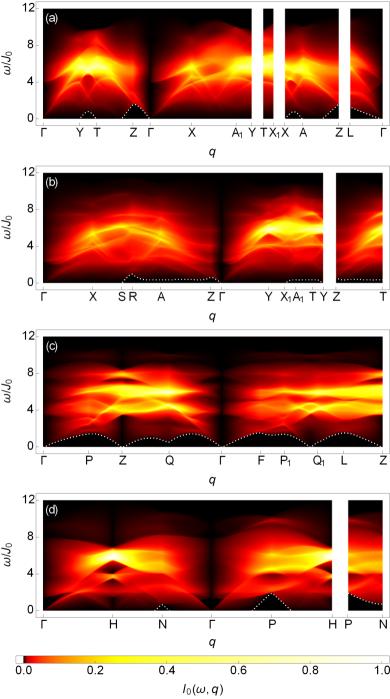
Figure 2: Lowest-order SC RIXS intensities of isotropic Kitaev models ($J_{x,y,z}=J_{0}$) on the (a) hyperhoneycomb, (b) stripyhoneycomb, (c) hyperhexagon, and (d) hyperoctagon lattices. In each case, the intensity is plotted along the high-symmetry path depicted in Fig. 3 and is normalized to be between $0$ and $1$. The dotted white line indicates a gap, below which the intensity is exactly zero.

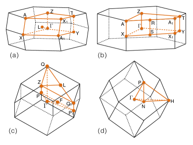
Figure 3: High-symmetry paths Setyawan-2010 within the Brillouin zones of the (a) hyperhoneycomb, (b) stripyhoneycomb, (c) hyperhexagon, and (d) hyperoctagon lattices.

Results and discussion.—At the isotropic point of each Kitaev model, the lowest-order SC RIXS response $I_{0}(\omega,\mathbf{q})$ is plotted in Fig. 2 along a high-symmetry path Setyawan-2010 within the Brillouin zone depicted in Fig. 3. For each model, the lack of sharp dispersion curves $\omega(\mathbf{q})$ indicates the absence of a one-fermion response, which is forbidden due to the fractionalized nature of the fermions. Instead, the SC RIXS response in the experimental regime is dominated by the two-fermion response in Eq. (8), and the overall energy dependence of each response is thus proportional to the two-fermion joint density of states plotted in the SM SM . Since the fermion bandwidth is $\approx 6J_{0}$, the bandwidth of the response is then $\approx 12J_{0}$.

Unlike the INS responses Smith-2015 ; Smith-2016 or, equivalently, the NSC RIXS responses, the SC RIXS responses in Fig. 2 are gapless and they have a pronounced momentum dependence. For each model, the low-energy (gapless) response is determined by the nodal structure of the fermions. Since the lowest-order SC RIXS processes create two fermions, the corresponding response is gapless at momentum $\mathbf{q}$ if there are gapless fermions at some momenta $\mathbf{k}_{1}$ and $\mathbf{k}_{2}$ such that $\mathbf{q}=\mathbf{k}_{1}+\mathbf{k}_{2}$. For the hyperhexagon model, the fermions are gapless at Weyl points, and the response is thus only gapless at particular points of the Brillouin zone. For the hyperhoneycomb and the stripyhoneycomb models, the fermions are gapless along a nodal line within the $\Gamma$-X-Y plane, and the response is thus gapless in most of the $\Gamma$-X-Y plane for both models and also in most of the Z-A-T plane for the hyperhoneycomb model. However, it is still gapped at a generic point of the Brillouin zone between these high-symmetry planes. For the hyperoctagon model, the fermions are gapless on a Fermi surface, and the response is thus gapless in most of the Brillouin zone.

For each model, the SC RIXS response in Fig. 2 is strongly suppressed around the $\Gamma$ point. Indeed, since $\mathcal{E}_{\mathbf{k}}^{\phantom{{\dagger}}}=-\mathcal{E}_{-\mathbf{k}}^{\phantom{{\dagger}}}$ is diagonal and $\mathcal{W}_{\mathbf{k}}^{\phantom{{\dagger}}}=\mathcal{W}_{-\mathbf{k}}^{*}$ is unitary, $(\mathcal{W}_{\mathbf{k}}^{{\dagger}}\cdot\mathcal{W}_{\mathbf{q}-\mathbf{k}}^{*})_{\mu\mu^{\prime}}=\delta_{\mu\mu^{\prime}}$ and hence $\mathcal{A}_{\mathbf{q},\mathbf{k}}$ is purely diagonal for $\mathbf{q}=\mathbf{0}$. The intensity $I_{0}(\omega,\mathbf{0})$ in Eq. (8) is then zero due to the Heaviside step functions and $\varepsilon_{-\mathbf{k},\mu}=-\varepsilon_{\mathbf{k},\mu}$. From a physical point of view, this suppression of the intensity can be understood for each model as a destructive interference between scattering processes at the two sublattices of the bipartite lattice, which in turn arises because each scattering process creates two fermions and each fermion involves a phase factor $i$ between the two sublattices (see the SM SM ). Remarkably, the phase factor $i$ indicates that the appropriate symmetry exchanging the two sublattices Footnote-2 acts projectively on the fermions as its action on them squares to $-1$ instead of $+1$ You-2012 . The strong suppression of the response around the $\Gamma$ point is thus a further signature of (symmetry) fractionalization.

For any actual material realizing a KSL phase, the Hamiltonian necessarily contains additional terms with respect to those in Eq. (1). In general, the high-energy response is robust against such perturbations, even beyond the phase transition into an ordered phase Banerjee-2016 , but the low-energy response of a generic KSL can be completely different from that of a pure Kitaev model Song-2016 . Nevertheless, we expect that the low-energy features of each SC RIXS response in Fig. 2 are valid for a generic point of the corresponding KSL phase as the low-energy physics is still governed by gapless (dressed) fermions with a particular nodal structure protected by the (projective) symmetries of the system Hermanns-2014 ; Hermanns-2015 ; O'Brien-2016 . In particular, for the hyperhoneycomb and the stripyhoneycomb KSLs, the nodal line remains within the $\Gamma$-X-Y plane as long as the two-fold rotation symmetry around any $z$ bond is intact Footnote-3 . The suppression of the response around the $\Gamma$ point is also expected to be a robust feature of each KSL phase as it occurs due to the particular way the symmetries fractionalize when acting on the fermions. In fact, it should be present for any KSL on a bipartite lattice, including the honeycomb KSL Halasz-2016 .

Summary.—Calculating the exact RIXS responses of four 3D Kitaev models, we have demonstrated that RIXS is a sensitive probe of the fractionalized excitations in 3D KSLs. In its NSC channels, RIXS measures the dynamical spin structure factor, while in its SC channel, it gives a complementary response, picking up exclusively the Majorana fermions. By looking at where the SC RIXS response is gapless, one can distinguish between the various nodal structures of Majorana fermions possible in 3D KSLs. Conversely, the suppression of the response around the $\Gamma$ point is expected to be a generic signature of all KSLs on a bipartite lattice.

We thank J. van den Brink, F. J. Burnell, J. T. Chalker, and J. Knolle for collaboration on closely related topics. G. B. H. is supported by the Gordon and Betty Moore Foundation’s EPiQS Initiative through Grant No. GBMF4304. N. B. P. is supported by the NSF Grant No. DMR-1511768 and is also grateful to the Perimeter Institute for their hospitality during the course of this work. Research at the Perimeter Institute is supported by the Government of Canada through Industry Canada and by the Province of Ontario through the Ministry of Economic Development and Innovation.

.1 Supplementary Material

I Tricoordinated lattices and Majorana-fermion Hamiltonians

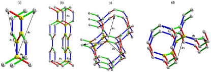
Figure 4: Primitive unit cells (yellow sites) and lattice vectors ($\mathbf{a}_{1,2,3}$) of the (a) hyperhoneycomb, (b) stripyhoneycomb, (c) hyperhexagon, and (d) hyperoctagon lattices. Different bond types $x$, $y$, and $z$ are marked by red, green, and blue, respectively.

Here we provide additional information on the four tricoordinated three-dimensional (3D) lattices as well as the corresponding Majorana-fermion Hamiltonians introduced in the main text. For each lattice, the unit cell and the lattice vectors are depicted in Fig. 4, the corresponding Majorana-fermion band structure is plotted in Fig. 5, while the one-fermion density of states and the two-fermion (joint) density of states are plotted in Figs. 6 and 7. In addition, the formal descriptions of the individual lattices and the precise forms of the corresponding Hamiltonian matrices $\hat{\mathcal{H}}_{\mathbf{k}}$ are given below. Note that we describe each lattice in an orthogonal coordinate system where the distance between two neighboring sites is assumed to be unity.

I.1 Hyperhoneycomb lattice

The hyperhoneycomb lattice is a face-centered orthorhombic lattice with four sites per (primitive) unit cell. The three lattice vectors of the face-centered orthorhombic lattice are given by

$$\mathbf{a}_{1}=\left(0,\sqrt{2},3\right),\quad\mathbf{a}_{2}=\left(1,0,3\right),\quad\mathbf{a}_{3}=\left(1,\sqrt{2},0\right),$$ (10)

while the coordinates of the four sites in each unit cell are

$$\mathbf{r}_{1}=\left(0,0,0\right),\quad\mathbf{r}_{2}=\left(\frac{1}{2},\frac{\sqrt{2}}{2},\frac{3}{2}\right),\quad\mathbf{r}_{3}=\left(0,0,1\right),\quad\mathbf{r}_{4}=\left(\frac{1}{2},\frac{\sqrt{2}}{2},\frac{5}{2}\right).$$ (11)

In the notation of Ref. [55] in the main text, the Brillouin zone is of type ORCF₁, and its high-symmetry points have coordinates

$$\Gamma=\left(0,0,0\right),\quad\textrm{A}=\left(\frac{25\pi}{36},0,\frac{\pi}{3}\right),\quad\textrm{A}_{1}=\left(\frac{11\pi}{36},\frac{\pi}{\sqrt{2}},0\right),\quad\textrm{L}=\left(\frac{\pi}{2},\frac{\pi}{2\sqrt{2}},\frac{\pi}{6}\right),\quad\textrm{T}=\left(0,\frac{\pi}{\sqrt{2}},\frac{\pi}{3}\right),$$

$$\textrm{X}=\left(\frac{29\pi}{36},0,0\right),\quad\textrm{X}_{1}=\left(\frac{7\pi}{36},\frac{\pi}{\sqrt{2}},\frac{\pi}{3}\right),\quad\textrm{Y}=\left(0,\frac{\pi}{\sqrt{2}},0\right),\quad\textrm{Z}=\left(0,0,\frac{\pi}{3}\right).$$ (12)

In the flux-free sector of the corresponding Kitaev model, the Hamiltonian matrix $\hat{\mathcal{H}}_{\mathbf{k}}$ takes the form

$$\hat{\mathcal{H}}_{\mathbf{k}}^{\phantom{{\dagger}}}=\Omega_{\mathbf{k}}^{{\dagger}}\cdot\check{\mathcal{H}}_{\mathbf{k}}^{\phantom{{\dagger}}}\cdot\Omega_{\mathbf{k}}^{\phantom{{\dagger}}},\qquad\check{\mathcal{H}}_{\mathbf{k}}^{\phantom{{\dagger}}}=\left(\begin{array}[]{cc}0&-i\check{\mathcal{M}}_{\mathbf{k}}^{\phantom{{\dagger}}}\\ i\check{\mathcal{M}}_{\mathbf{k}}^{{\dagger}}&0\end{array}\right),\qquad\check{\mathcal{M}}_{\mathbf{k}}^{\phantom{{\dagger}}}=\left(\begin{array}[]{cc}J_{z}&J_{x}e^{-ik_{2}}+J_{y}e^{-ik_{1}}\\ J_{x}+J_{y}e^{ik_{3}}&J_{z}\end{array}\right),$$ (13)

where $k_{j}\equiv\mathbf{k}\cdot\mathbf{a}_{j}$ with $j=1,2,3$, while $\Omega_{\mathbf{k}}=\mathrm{diag}\{\exp(i\mathbf{k}\cdot\mathbf{r}_{j})\}_{j=1,2,3,4}$.

I.2 Stripyhoneycomb lattice

The stripyhoneycomb lattice is a base-centered orthorhombic lattice with eight sites per (primitive) unit cell. The three lattice vectors of the base-centered orthorhombic lattice are given by

$$\mathbf{a}_{1}=\left(1,-\sqrt{2},0\right),\quad\mathbf{a}_{2}=\left(1,\sqrt{2},0\right),\quad\mathbf{a}_{3}=\left(0,0,6\right),$$ (14)

while the coordinates of the eight sites in each unit cell are

$$\mathbf{r}_{1}=\left(0,0,0\right),\quad\mathbf{r}_{2}=\left(\frac{1}{2},\frac{\sqrt{2}}{2},\frac{3}{2}\right),\quad\mathbf{r}_{3}=\left(0,0,3\right),\quad\mathbf{r}_{4}=\left(\frac{1}{2},-\frac{\sqrt{2}}{2},\frac{9}{2}\right),$$

$$\mathbf{r}_{5}=\left(0,0,1\right),\quad\mathbf{r}_{6}=\left(\frac{1}{2},\frac{\sqrt{2}}{2},\frac{5}{2}\right),\quad\mathbf{r}_{7}=\left(0,0,4\right),\quad\mathbf{r}_{8}=\left(\frac{1}{2},-\frac{\sqrt{2}}{2},\frac{11}{2}\right).$$ (15)

In the notation of Ref. [55] in the main text, the Brillouin zone is of type ORCC, and its high-symmetry points have coordinates

$$\Gamma=\left(0,0,0\right),\quad\textrm{A}=\left(\frac{3\pi}{4},0,\frac{\pi}{6}\right),\quad\textrm{A}_{1}=\left(\frac{\pi}{4},\frac{\pi}{\sqrt{2}},\frac{\pi}{6}\right),\quad\textrm{R}=\left(\frac{\pi}{2},\frac{\pi}{2\sqrt{2}},\frac{\pi}{6}\right),\quad\textrm{S}=\left(\frac{\pi}{2},\frac{\pi}{2\sqrt{2}},0\right),\quad\textrm{T}=\left(0,\frac{\pi}{\sqrt{2}},\frac{\pi}{6}\right),$$

$$\textrm{X}=\left(\frac{3\pi}{4},0,0\right),\quad\textrm{X}_{1}=\left(\frac{\pi}{4},\frac{\pi}{\sqrt{2}},0\right),\quad\textrm{Y}=\left(0,\frac{\pi}{\sqrt{2}},0\right),\quad\textrm{Z}=\left(0,0,\frac{\pi}{6}\right).$$ (16)

In the flux-free sector of the corresponding Kitaev model, the Hamiltonian matrix $\hat{\mathcal{H}}_{\mathbf{k}}$ takes the form

$$\qquad\qquad\qquad\hat{\mathcal{H}}_{\mathbf{k}}^{\phantom{{\dagger}}}=\Omega_{\mathbf{k}}^{{\dagger}}\cdot\check{\mathcal{H}}_{\mathbf{k}}^{\phantom{{\dagger}}}\cdot\Omega_{\mathbf{k}}^{\phantom{{\dagger}}},\qquad\check{\mathcal{H}}_{\mathbf{k}}^{\phantom{{\dagger}}}=\left(\begin{array}[]{cc}0&-i\check{\mathcal{M}}_{\mathbf{k}}^{\phantom{{\dagger}}}\\ i\check{\mathcal{M}}_{\mathbf{k}}^{{\dagger}}&0\end{array}\right),$$ (19)

$$\check{\mathcal{M}}_{\mathbf{k}}^{\phantom{{\dagger}}}=\left(\begin{array}[]{cccc}J_{z}&0&0&J_{x}e^{-ik_{1}-ik_{3}}+J_{y}e^{-ik_{3}}\\ J_{x}+J_{y}e^{ik_{2}}&J_{z}&0&0\\ 0&J_{x}e^{-ik_{2}}+J_{y}&J_{z}&0\\ 0&0&J_{x}+J_{y}e^{ik_{1}}&J_{z}\end{array}\right),$$ (24)

where $k_{j}\equiv\mathbf{k}\cdot\mathbf{a}_{j}$ with $j=1,2,3$, while $\Omega_{\mathbf{k}}=\mathrm{diag}\{\exp(i\mathbf{k}\cdot\mathbf{r}_{j})\}_{j=1,2,\ldots,8}$.

I.3 Hyperhexagon lattice

The hyperhexagon lattice is a simple rhombohedral lattice with six sites per (primitive) unit cell. The three lattice vectors of the rhombohedral lattice are given by

$$\mathbf{a}_{1}=\left(0,-\frac{5}{\sqrt{3}},\sqrt{\frac{2}{3}}\right),\quad\mathbf{a}_{2}=\left(-\frac{5}{2},\frac{5}{2\sqrt{3}},\sqrt{\frac{2}{3}}\right),\quad\mathbf{a}_{3}=\left(\frac{5}{2},\frac{5}{2\sqrt{3}},\sqrt{\frac{2}{3}}\right),$$ (25)

while the coordinates of the six sites in each unit cell are

$$\mathbf{r}_{1}=\left(0,0,0\right),\quad\mathbf{r}_{2}=\left(\frac{1}{2},\frac{1}{2\sqrt{3}},2\sqrt{\frac{2}{3}}\right),\quad\mathbf{r}_{3}=\left(1,\sqrt{3},\sqrt{6}\right),\quad\mathbf{r}_{4}=\left(\frac{1}{2},-\frac{1}{2\sqrt{3}},\sqrt{\frac{2}{3}}\right),$$

$$\mathbf{r}_{5}=\left(1,\frac{2}{\sqrt{3}},2\sqrt{\frac{2}{3}}\right),\quad\mathbf{r}_{6}=\left(\frac{3}{2},\frac{5}{2\sqrt{3}},4\sqrt{\frac{2}{3}}\right).$$ (26)

In the notation of Ref. [55] in the main text, the Brillouin zone is of type RHL₂, and its high-symmetry points have coordinates

$$\Gamma=\left(0,0,0\right),\quad\textrm{F}=\left(\frac{\pi}{5},-\frac{\sqrt{3}\pi}{5},0\right),\quad\textrm{L}=\left(0,-\frac{2\pi}{5\sqrt{3}},\frac{\pi}{\sqrt{6}}\right),\quad\textrm{P}=\left(\frac{2\pi}{5},-\frac{2\pi}{5\sqrt{3}},\frac{2\pi}{25}\sqrt{\frac{2}{3}}\right),\quad\textrm{P}_{1}=\left(0,-\frac{4\pi}{5\sqrt{3}},-\frac{2\pi}{25}\sqrt{\frac{2}{3}}\right),$$

$$\textrm{Q}=\left(0,0,\frac{11\pi}{25}\sqrt{\frac{3}{2}}\right),\quad\textrm{Q}_{1}=\left(0,-\frac{4\pi}{5\sqrt{3}},\frac{17\pi}{25\sqrt{6}}\right),\quad\textrm{Z}=\left(\frac{2\pi}{5},-\frac{2\pi}{5\sqrt{3}},\frac{\pi}{\sqrt{6}}\right).$$ (27)

In the ground-state flux sector of the corresponding Kitaev model, the Hamiltonian matrix $\hat{\mathcal{H}}_{\mathbf{k}}$ takes the form

$$\qquad\qquad\hat{\mathcal{H}}_{\mathbf{k}}^{\phantom{{\dagger}}}=\Omega_{\mathbf{k}}^{{\dagger}}\cdot\check{\mathcal{H}}_{\mathbf{k}}^{\phantom{{\dagger}}}\cdot\Omega_{\mathbf{k}}^{\phantom{{\dagger}}},\\$$ (28)

$$\check{\mathcal{H}}_{\mathbf{k}}^{\phantom{{\dagger}}}=i\left(\begin{array}[]{cccccc}0&J_{x}e^{-ik_{1}-ik_{2}-ik_{3}}&0&J_{z}&0&J_{y}e^{-ik_{1}-ik_{2}-2ik_{3}}\\ -J_{x}e^{ik_{1}+ik_{2}+ik_{3}}&0&0&J_{y}&J_{z}&0\\ 0&0&0&J_{x}e^{ik_{2}+ik_{3}}&J_{y}&J_{z}\\ -J_{z}&-J_{y}&-J_{x}e^{-ik_{2}-ik_{3}}&0&0&0\\ 0&-J_{z}&-J_{y}&0&0&-J_{x}e^{-ik_{1}-ik_{2}-ik_{3}}\\ -J_{y}e^{ik_{1}+ik_{2}+2ik_{3}}&0&-J_{z}&0&J_{x}e^{ik_{1}+ik_{2}+ik_{3}}&0\end{array}\right),$$ (35)

where $k_{j}\equiv\mathbf{k}\cdot\mathbf{a}_{j}$ with $j=1,2,3$, while $\Omega_{\mathbf{k}}=\mathrm{diag}\{\exp(i\mathbf{k}\cdot\mathbf{r}_{j})\}_{j=1,2,\ldots,6}$.

Figure 5: Majorana-fermion (spinon) band structures of isotropic Kitaev models ($J_{x,y,z}=J_{0}$) on the (a) hyperhoneycomb, (b) stripyhoneycomb, (c) hyperhexagon, and (d) hyperoctagon lattices. Note that only the fermions with positive energies $\varepsilon_{\mathbf{k}}>0$ are physical while the ones with negative energies $\varepsilon_{\mathbf{k}}<0$ at momentum $\mathbf{k}$ are identified with physical fermions at momentum $-\mathbf{k}$.

Figure 6: One-fermion densities of states (1-DOS) of isotropic Kitaev models ($J_{x,y,z}=J_{0}$) on the (a) hyperhoneycomb, (b) stripyhoneycomb, (c) hyperhexagon, and (d) hyperoctagon lattices. In each case, the density of states is normalized such that its integral is unity.

Figure 7: Two-fermion densities of states (2-DOS) of isotropic Kitaev models ($J_{x,y,z}=J_{0}$) on the (a) hyperhoneycomb, (b) stripyhoneycomb, (c) hyperhexagon, and (d) hyperoctagon lattices. In each case, the density of states is normalized such that its integral is unity.

I.4 Hyperoctagon lattice

The hyperoctagon lattice is a body-centered cubic lattice with four sites per (primitive) unit cell. The three lattice vectors of the body-centered cubic lattice are given by

$$\mathbf{a}_{1}=\left(-\sqrt{2},\sqrt{2},\sqrt{2}\right),\quad\mathbf{a}_{2}=\left(\sqrt{2},-\sqrt{2},\sqrt{2}\right),\quad\mathbf{a}_{3}=\left(\sqrt{2},\sqrt{2},-\sqrt{2}\right),$$ (36)

while the coordinates of the four sites in each unit cell are

$$\mathbf{r}_{1}=\left(0,0,0\right),\quad\mathbf{r}_{2}=\left(\sqrt{2},\frac{1}{\sqrt{2}},-\frac{1}{\sqrt{2}}\right),\quad\mathbf{r}_{3}=\left(\frac{1}{\sqrt{2}},0,-\frac{1}{\sqrt{2}}\right),\quad\mathbf{r}_{4}=\left(\frac{3}{\sqrt{2}},\frac{1}{\sqrt{2}},0\right).$$ (37)

In the notation of Ref. [55] in the main text, the Brillouin zone is of type BCC, and its high-symmetry points have coordinates

$$\Gamma=\left(0,0,0\right),\quad\textrm{H}=\left(0,\frac{\pi}{\sqrt{2}},0\right),\quad\textrm{N}=\left(\frac{\pi}{2\sqrt{2}},\frac{\pi}{2\sqrt{2}},0\right),\quad\textrm{P}=\left(\frac{\pi}{2\sqrt{2}},\frac{\pi}{2\sqrt{2}},\frac{\pi}{2\sqrt{2}}\right).$$ (38)

In the flux-free sector of the corresponding Kitaev model, the Hamiltonian matrix $\hat{\mathcal{H}}_{\mathbf{k}}$ takes the form

$$\hat{\mathcal{H}}_{\mathbf{k}}^{\phantom{{\dagger}}}=\Omega_{\mathbf{k}}^{{\dagger}}\cdot\check{\mathcal{H}}_{\mathbf{k}}^{\phantom{{\dagger}}}\cdot\Omega_{\mathbf{k}}^{\phantom{{\dagger}}},\qquad\check{\mathcal{H}}_{\mathbf{k}}^{\phantom{{\dagger}}}=i\left(\begin{array}[]{cccc}0&-J_{x}e^{-ik_{3}}&-J_{y}&-J_{z}e^{-ik_{2}-ik_{3}}\\ J_{x}e^{ik_{3}}&0&-J_{z}&J_{y}\\ J_{y}&J_{z}&0&-J_{x}e^{-ik_{1}-ik_{2}-ik_{3}}\\ J_{z}e^{ik_{2}+ik_{3}}&-J_{y}&J_{x}e^{ik_{1}+ik_{2}+ik_{3}}&0\end{array}\right),$$ (39)

where $k_{j}\equiv\mathbf{k}\cdot\mathbf{a}_{j}$ with $j=1,2,3$, while $\Omega_{\mathbf{k}}=\mathrm{diag}\{\exp(i\mathbf{k}\cdot\mathbf{r}_{j})\}_{j=1,2,3,4}$.

II Scattering amplitude in the spin-conserving channel

Here we evaluate the spin-conserving RIXS amplitude $A_{0}(m,\mathbf{q})$ in Eq. (7) of the main text between the ground state $|0\rangle$ and a generic final state $|m\rangle=\psi_{\mathbf{q}-\mathbf{k},\mu^{\prime}}^{{\dagger}}\psi_{\mathbf{k},\mu}^{{\dagger}}|0\rangle$ containing two fermions. The inverse of Eq. (4) in the main text is given by

$$c_{\mathbf{r}\in\nu}^{\phantom{{\dagger}}}=\sqrt{\frac{2}{N}}\sum_{\mathbf{k},\mu}\left(\mathcal{W}_{\mathbf{k}}^{{\dagger}}\right)_{\mu\nu}\psi_{\mathbf{k},\mu}^{{\dagger}}\,e^{-i\mathbf{k}\cdot\mathbf{r}},$$ (40)

and the RIXS amplitude in Eq. (7) of the main text reads

$$A_{0}(m,\mathbf{q}) \propto \sum_{\nu,\nu^{\prime}}\,\sum_{\mathbf{r}\in\nu}\,\sum_{\mathbf{r}^{\prime}\in\nu^{\prime}}e^{i\mathbf{q}\cdot\mathbf{r}}\,\mathcal{H}_{\mathbf{r},\mathbf{r}^{\prime}}^{\phantom{{\dagger}}}\langle 0|\psi_{\mathbf{k},\mu}^{\phantom{{\dagger}}}\psi_{\mathbf{q}-\mathbf{k},\mu^{\prime}}^{\phantom{{\dagger}}}c_{\mathbf{r}}^{\phantom{{\dagger}}}c_{\mathbf{r}^{\prime}}^{\phantom{{\dagger}}}|0\rangle$$ (41)

$$= \frac{2}{N}\sum_{\nu,\nu^{\prime}}\,\sum_{\mathbf{r}\in\nu}\,\sum_{\mathbf{r}^{\prime}\in\nu^{\prime}}e^{i\mathbf{q}\cdot\mathbf{r}}\,\mathcal{H}_{\mathbf{r},\mathbf{r}^{\prime}}^{\phantom{{\dagger}}}\bigg{[}\langle 0|\psi_{\mathbf{k},\mu}^{\phantom{{\dagger}}}\psi_{\mathbf{q}-\mathbf{k},\mu^{\prime}}^{\phantom{{\dagger}}}\psi_{\mathbf{k},\mu}^{{\dagger}}\psi_{\mathbf{q}-\mathbf{k},\mu^{\prime}}^{{\dagger}}|0\rangle\left(\mathcal{W}_{\mathbf{k}}^{{\dagger}}\right)_{\mu\nu}\left(\mathcal{W}_{\mathbf{q}-\mathbf{k}}^{{\dagger}}\right)_{\mu^{\prime}\nu^{\prime}}e^{-i\mathbf{k}\cdot\mathbf{r}-i(\mathbf{q}-\mathbf{k})\cdot\mathbf{r}^{\prime}}$$

$$+\,\langle 0|\psi_{\mathbf{k},\mu}^{\phantom{{\dagger}}}\psi_{\mathbf{q}-\mathbf{k},\mu^{\prime}}^{\phantom{{\dagger}}}\psi_{\mathbf{q}-\mathbf{k},\mu^{\prime}}^{{\dagger}}\psi_{\mathbf{k},\mu}^{{\dagger}}|0\rangle\left(\mathcal{W}_{\mathbf{q}-\mathbf{k}}^{{\dagger}}\right)_{\mu^{\prime}\nu}\left(\mathcal{W}_{\mathbf{k}}^{{\dagger}}\right)_{\mu\nu^{\prime}}e^{-i(\mathbf{q}-\mathbf{k})\cdot\mathbf{r}-i\mathbf{k}\cdot\mathbf{r}^{\prime}}\bigg{]}.$$

Using Eq. (5) of the main text, the RIXS amplitude then becomes

$$A_{0}(m,\mathbf{q}) \propto \sum_{\nu,\nu^{\prime}}\left[\Big{(}\hat{\mathcal{H}}_{\mathbf{k}}^{*}\Big{)}_{\nu\nu^{\prime}}\left(\mathcal{W}_{\mathbf{q}-\mathbf{k}}^{{\dagger}}\right)_{\mu^{\prime}\nu}\left(\mathcal{W}_{\mathbf{k}}^{{\dagger}}\right)_{\mu\nu^{\prime}}-\Big{(}\hat{\mathcal{H}}_{\mathbf{q}-\mathbf{k}}^{*}\Big{)}_{\nu\nu^{\prime}}\left(\mathcal{W}_{\mathbf{k}}^{{\dagger}}\right)_{\mu\nu}\left(\mathcal{W}_{\mathbf{q}-\mathbf{k}}^{{\dagger}}\right)_{\mu^{\prime}\nu^{\prime}}\right]$$ (42)

$$= \left[\mathcal{W}_{\mathbf{k}}^{{\dagger}}\cdot\hat{\mathcal{H}}_{\mathbf{k}}^{\phantom{{\dagger}}}\cdot\mathcal{W}_{\mathbf{q}-\mathbf{k}}^{*}-\mathcal{W}_{\mathbf{k}}^{{\dagger}}\cdot\hat{\mathcal{H}}_{\mathbf{q}-\mathbf{k}}^{*}\cdot\mathcal{W}_{\mathbf{q}-\mathbf{k}}^{*}\right]_{\mu\mu^{\prime}}.$$

Note that the relative minus sign between the two terms arises because the two fermions $\psi_{\mathbf{k},\mu}^{{\dagger}}$ and $\psi_{\mathbf{q}-\mathbf{k},\mu^{\prime}}^{{\dagger}}$ are created in opposite orders. Finally, due to $\hat{\mathcal{H}}_{\mathbf{k}}^{\phantom{{\dagger}}}=\mathcal{W}_{\mathbf{k}}^{\phantom{{\dagger}}}\cdot\mathcal{E}_{\mathbf{k}}^{\phantom{{\dagger}}}\cdot\mathcal{W}_{\mathbf{k}}^{{\dagger}}$ and $\mathcal{W}_{\mathbf{k}}^{\phantom{{\dagger}}}\cdot\mathcal{W}_{\mathbf{k}}^{{\dagger}}=1$, the RIXS amplitude in Eq. (42) takes the form

$$A_{0}(m,\mathbf{q})\propto\left[\mathcal{E}_{\mathbf{k}}^{\phantom{{\dagger}}}\cdot\mathcal{W}_{\mathbf{k}}^{{\dagger}}\cdot\mathcal{W}_{\mathbf{q}-\mathbf{k}}^{*}-\mathcal{W}_{\mathbf{k}}^{{\dagger}}\cdot\mathcal{W}_{\mathbf{q}-\mathbf{k}}^{*}\cdot\mathcal{E}_{\mathbf{q}-\mathbf{k}}^{\phantom{{\dagger}}}\right]_{\mu\mu^{\prime}}.$$ (43)

This result is identical to the appropriate matrix element of $\mathcal{A}_{\mathbf{q},\mathbf{k}}$ in Eq. (9) of the main text.

III Consequences of the bipartite lattice structure

For a Kitaev model on a bipartite lattice, where the $n=2m$ sites per unit cell can be divided into two classes $\nu_{A}=1,\ldots,m$ and $\nu_{B}=m+1,\ldots,2m$ such that any $A$ ($B$) site only neighbors $B$ ($A$) sites, the matrices $\hat{\mathcal{H}}_{\mathbf{k}}^{\phantom{{\dagger}}}$, $\mathcal{E}_{\mathbf{k}}^{\phantom{{\dagger}}}$, and $\mathcal{W}_{\mathbf{k}}^{\phantom{{\dagger}}}$ take the forms

$$\hat{\mathcal{H}}_{\mathbf{k}}^{\phantom{{\dagger}}}=\left(\begin{array}[]{cc}0&-i\hat{\mathcal{M}}_{\mathbf{k}}^{\phantom{{\dagger}}}\\ i\hat{\mathcal{M}}_{\mathbf{k}}^{{\dagger}}&0\end{array}\right),\quad\mathcal{E}_{\mathbf{k}}^{\phantom{{\dagger}}}=\left(\begin{array}[]{cc}\Lambda_{\mathbf{k}}^{\phantom{{\dagger}}}&0\\ 0&-\Lambda_{\mathbf{k}}^{\phantom{{\dagger}}}\end{array}\right),\quad\mathcal{W}_{\mathbf{k}}^{\phantom{{\dagger}}}=\frac{1}{\sqrt{2}}\left(\begin{array}[]{cc}\mathcal{U}_{\mathbf{k}}^{\phantom{{\dagger}}}&\mathcal{U}_{\mathbf{k}}^{\phantom{{\dagger}}}\\ i\mathcal{V}_{\mathbf{k}}^{\phantom{{\dagger}}}&-i\mathcal{V}_{\mathbf{k}}^{\phantom{{\dagger}}}\end{array}\right),$$ (44)

where the diagonal matrix $\Lambda_{\mathbf{k}}^{\phantom{{\dagger}}}$ and the unitary matrices $\mathcal{U}_{\mathbf{k}}^{\phantom{{\dagger}}}$ and $\mathcal{V}_{\mathbf{k}}^{\phantom{{\dagger}}}$ can be obtained by taking the singular-value decomposition $\hat{\mathcal{M}}_{\mathbf{k}}^{\phantom{{\dagger}}}=\mathcal{U}_{\mathbf{k}}^{\phantom{{\dagger}}}\cdot\Lambda_{\mathbf{k}}^{\phantom{{\dagger}}}\cdot\mathcal{V}_{\mathbf{k}}^{{\dagger}}$. Since the singular values $\lambda_{\mathbf{k},\mu}=(\Lambda_{\mathbf{k}})_{\mu\mu}$ are positive by definition, the physical (positive-energy) fermions are then the ones with $\mu=1,\ldots,m$ for all momenta $\mathbf{k}$. Furthermore, $\hat{\mathcal{M}}_{-\mathbf{k}}^{\phantom{{\dagger}}}=\hat{\mathcal{M}}_{\mathbf{k}}^{*}$ implies $\Lambda_{-\mathbf{k}}^{\phantom{{\dagger}}}=\Lambda_{\mathbf{k}}^{\phantom{{\dagger}}}$ as well as $\mathcal{U}_{-\mathbf{k}}^{\phantom{{\dagger}}}=\mathcal{U}_{\mathbf{k}}^{*}$ and $\mathcal{V}_{-\mathbf{k}}^{\phantom{{\dagger}}}=\mathcal{V}_{\mathbf{k}}^{*}$. We remark that all four Kitaev models in the main text are defined on bipartite lattices. For the hyperhoneycomb and the stripyhoneycomb models, the bipartite structure of the lattice is compatible with the unit cell, and the Hamiltonian matrices in Eqs. (13) and (24) readily take the form of $\hat{\mathcal{H}}_{\mathbf{k}}^{\phantom{{\dagger}}}$ in Eq. (44). For the hyperhexagon and the hyperoctagon models, the bipartite structure is not compatible with the original unit cell of the lattice. However, if we artificially double the unit cell, it becomes compatible with the bipartite structure, and the enlarged Hamiltonian matrix takes the form of $\hat{\mathcal{H}}_{\mathbf{k}}^{\phantom{{\dagger}}}$ in Eq. (44).

If the bipartite lattice of the Kitaev model consists of $N$ unit cells, the physical (positive-energy) fermions with band index $\mu=1,\ldots,m$ in Eq. (4) of the main text can be written as

$$\psi_{\mathbf{k},\mu}^{{\dagger}}=\frac{1}{2\sqrt{N}}\sum_{\nu=1}^{m}\left[\big{(}\mathcal{U}_{\mathbf{k}}^{\phantom{{\dagger}}}\big{)}_{\nu\mu}\sum_{\mathbf{r}\in\nu_{A}}c_{\mathbf{r}}^{\phantom{{\dagger}}}\,e^{i\mathbf{k}\cdot\mathbf{r}}+i\big{(}\mathcal{V}_{\mathbf{k}}^{\phantom{{\dagger}}}\big{)}_{\nu\mu}\sum_{\mathbf{r}\in\nu_{B}}c_{\mathbf{r}}^{\phantom{{\dagger}}}\,e^{i\mathbf{k}\cdot\mathbf{r}}\right],$$ (45)

where $\nu_{A}=\nu$ and $\nu_{B}=\nu+m$ for each $\nu=1,\ldots,m$. Restricting our attention to these physical fermions, the spin-conserving RIXS amplitude in Eq. (43) is then given by

$$A_{0}(m,\mathbf{q})\propto\left[\Lambda_{\mathbf{k}}^{\phantom{{\dagger}}}\cdot\left(\mathcal{U}_{\mathbf{k}}^{{\dagger}}\cdot\mathcal{U}_{\mathbf{q}-\mathbf{k}}^{*}-\mathcal{V}_{\mathbf{k}}^{{\dagger}}\cdot\mathcal{V}_{\mathbf{q}-\mathbf{k}}^{*}\right)-\left(\mathcal{U}_{\mathbf{k}}^{{\dagger}}\cdot\mathcal{U}_{\mathbf{q}-\mathbf{k}}^{*}-\mathcal{V}_{\mathbf{k}}^{{\dagger}}\cdot\mathcal{V}_{\mathbf{q}-\mathbf{k}}^{*}\right)\cdot\Lambda_{\mathbf{q}-\mathbf{k}}^{\phantom{{\dagger}}}\right]_{\mu\mu^{\prime}}.$$ (46)

The terms proportional to $\mathcal{U}_{\mathbf{k}}^{{\dagger}}\cdot\mathcal{U}_{\mathbf{q}-\mathbf{k}}^{*}$ capture scattering processes at sublattice $A$ sites, while the terms proportional to $\mathcal{V}_{\mathbf{k}}^{{\dagger}}\cdot\mathcal{V}_{\mathbf{q}-\mathbf{k}}^{*}$ capture scattering processes at sublattice $B$ sites. For $\mathbf{q}=\mathbf{0}$, the scattering processes in each sublattice interfere constructively because $\mathcal{U}_{\mathbf{k}}^{{\dagger}}\cdot\mathcal{U}_{-\mathbf{k}}^{*}=\mathcal{V}_{\mathbf{k}}^{{\dagger}}\cdot\mathcal{V}_{-\mathbf{k}}^{*}=1$. However, there is a destructive interference between the two sublattices due to the relative minus sign in Eq. (46), and the spin-conserving RIXS intensity $I_{0}(\omega,\mathbf{q})$ in Eq. (8) of the main text is thus zero. Importantly, this relative minus sign between the two sublattices arises because each scattering process creates two fermions and each fermion involves a phase factor $i$ between the two sublattices [see Eq. (45)].

References

• (1) L. Balents, Nature 464, 199 (2010).
• (2) L. Savary and L. Balents, Rep. Prog. Phys. 80, 016502 (2016).
• (3) A. Y. Kitaev, Ann. Phys. 321, 2 (2006).
• (4) S. Mandal and N. Surendran, Phys. Rev. B 79, 024426 (2009).
• (5) M. Hermanns and S. Trebst, Phys. Rev. B 89, 235102 (2014).
• (6) M. Hermanns, K. O’Brien, and S. Trebst, Phys. Rev. Lett. 114, 157202 (2015).
• (7) K. O’Brien, M. Hermanns, and S. Trebst, Phys. Rev. B 93, 085101 (2016).
• (8) M. Hermanns, I. Kimchi, and J. Knolle, arXiv:1705.01740.
• (9) G. Jackeli and G. Khaliullin, Phys. Rev. Lett. 102, 017205 (2009).
• (10) J. Chaloupka, G. Jackeli, and G. Khaliullin, Phys. Rev. Lett. 105, 027204 (2010).
• (11) J. Chaloupka, G. Jackeli, and G. Khaliullin, Phys. Rev. Lett. 110, 097204 (2013).
• (12) S. Trebst, arXiv:1701.07056.
• (13) Y. Singh and P. Gegenwart, Phys. Rev. B 82, 064412 (2010).
• (14) X. Liu, T. Berlijn, W.-G. Yin, W. Ku, A. Tsvelik, Y.-J. Kim, H. Gretarsson, Y. Singh, P. Gegenwart, and J. P. Hill, Phys. Rev. B 83, 220403(R) (2011).
• (15) Y. Singh, S. Manni, J. Reuther, T. Berlijn, R. Thomale, W. Ku, S. Trebst, and P. Gegenwart, Phys. Rev. Lett. 108, 127203 (2012).
• (16) S. K. Choi, R. Coldea, A. N. Kolmogorov, T. Lancaster, I. I. Mazin, S. J. Blundell, P. G. Radaelli, Y. Singh, P. Gegenwart, K. R. Choi, S.-W. Cheong, P. J. Baker, C. Stock, and J. Taylor, Phys. Rev. Lett. 108, 127204 (2012).
• (17) F. Ye, S. Chi, H. Cao, B. C. Chakoumakos, J. A. Fernandez-Baca, R. Custelcean, T. F. Qi, O. B. Korneta, and G. Cao, Phys. Rev. B 85, 180403(R) (2012).
• (18) R. Comin, G. Levy, B. Ludbrook, Z.-H. Zhu, C. N. Veenstra, J. A. Rosen, Y. Singh, P. Gegenwart, D. Stricker, J. N. Hancock, D. van der Marel, I. S. Elfimov, and A. Damascelli, Phys. Rev. Lett. 109, 266406 (2012).
• (19) S. C. Williams, R. D. Johnson, F. Freund, S. Choi, A. Jesche, I. Kimchi, S. Manni, A. Bombardi, P. Manuel, P. Gegenwart, and R. Coldea, Phys. Rev. B 93, 195158 (2016).
• (20) K. W. Plumb, J. P. Clancy, L. J. Sandilands, V. V. Shankar, Y. F. Hu, K. S. Burch, H.-Y. Kee, and Y.-J. Kim, Phys. Rev. B 90, 041112(R) (2014).
• (21) L. J. Sandilands, Y. Tian, K. W. Plumb, Y.-J. Kim, and K. S. Burch, Phys. Rev. Lett. 114, 147201 (2015).
• (22) J. A. Sears, M. Songvilay, K. W. Plumb, J. P. Clancy, Y. Qiu, Y. Zhao, D. Parshall, and Y.-J. Kim, Phys. Rev. B 91, 144420 (2015).
• (23) M. Majumder, M. Schmidt, H. Rosner, A. A. Tsirlin, H. Yasuoka, and M. Baenitz, Phys. Rev. B 91, 180401(R) (2015).
• (24) R. D. Johnson, S. C. Williams, A. A. Haghighirad, J. Singleton, V. Zapf, P. Manuel, I. I. Mazin, Y. Li, H. O. Jeschke, R. Valentí, and R. Coldea, Phys. Rev. B 92, 235119 (2015).
• (25) L. J. Sandilands, Y. Tian, A. A. Reijnders, H.-S. Kim, K. W. Plumb, Y.-J. Kim, H.-Y. Kee, and K. S. Burch, Phys. Rev. B 93, 075144 (2016).
• (26) A. Banerjee, C. A. Bridges, J.-Q. Yan, A. A. Aczel, L. Li, M. B. Stone, G. E. Granroth, M. D. Lumsden, Y. Yiu, J. Knolle, S. Bhattacharjee, D. L. Kovrizhin, R. Moessner, D. A. Tennant, D. G. Mandrus, and S. E. Nagler, Nat. Mater. 15, 733 (2016).
• (27) K. A. Modic, T. E. Smidt, I. Kimchi, N. P. Breznay, A. Biffin, S. Choi, R. D. Johnson, R. Coldea, P. Watkins-Curry, G. T. McCandless, J. Y. Chan, F. Gandara, Z. Islam, A. Vishwanath, A. Shekhter, R. D. McDonald, and J. G. Analytis, Nat. Commun. 5, 4203 (2014).
• (28) A. Biffin, R. D. Johnson, I. Kimchi, R. Morris, A. Bombardi, J. G. Analytis, A. Vishwanath, and R. Coldea, Phys. Rev. Lett. 113, 197201 (2014).
• (29) A. Biffin, R. D. Johnson, S. Choi, F. Freund, S. Manni, A. Bombardi, P. Manuel, P. Gegenwart, and R. Coldea, Phys. Rev. B 90, 205116 (2014).
• (30) T. Takayama, A. Kato, R. Dinnebier, J. Nuss, H. Kono, L. S. I. Veiga, G. Fabbris, D. Haskel, and H. Takagi, Phys. Rev. Lett. 114, 077202 (2015).
• (31) J. Knolle, D. L. Kovrizhin, J. T. Chalker, and R. Moessner, Phys. Rev. Lett. 112, 207203 (2014).
• (32) J. Knolle, D. L. Kovrizhin, J. T. Chalker, and R. Moessner, Phys. Rev. B 92, 115127 (2015).
• (33) A. Smith, J. Knolle, D. L. Kovrizhin, J. T. Chalker, and R. Moessner, Phys. Rev. B 92, 180408(R) (2015).
• (34) A. Smith, J. Knolle, D. L. Kovrizhin, J. T. Chalker, and R. Moessner, Phys. Rev. B 93, 235146 (2016).
• (35) J. Knolle, G.-W. Chern, D. L. Kovrizhin, R. Moessner, and N. B. Perkins, Phys. Rev. Lett. 113, 187201 (2014).
• (36) B. Perreault, J. Knolle, N. B. Perkins, and F. J. Burnell, Phys. Rev. B 92, 094439 (2015).
• (37) B. Perreault, J. Knolle, N. B. Perkins, and F. J. Burnell, Phys. Rev. B 94, 060408(R) (2016).
• (38) B. Perreault, J. Knolle, N. B. Perkins, and F. J. Burnell, Phys. Rev. B 94, 104427 (2016).
• (39) A. Glamazda, P. Lemmens, S.-H. Do, Y. S. Choi, and K.-Y. Choi, Nat. Commun. 7, 12286 (2016).
• (40) W.-H. Ko and P. A. Lee, Phys. Rev. B 84, 125102 (2011).
• (41) L. Savary and T. Senthil, arXiv:1506.04752.
• (42) G. B. Halász, N. B. Perkins, and J. van den Brink, Phys. Rev. Lett. 117, 127203 (2016).
• (43) L. J. P. Ament, G. Khaliullin, and J. van den Brink, Phys. Rev. B 84, 020403(R) (2011).
• (44) B. J. Kim and G. Khaliullin, arXiv:1705.00215.
• (45) L. J. P. Ament, M. van Veenendaal, T. P. Devereaux, J. P. Hill, and J. van den Brink, Rev. Mod. Phys. 83, 705 (2011).
• (46) A. J. Willans, J. T. Chalker, and R. Moessner, Phys. Rev. Lett. 104, 237203 (2010).
• (47) A. J. Willans, J. T. Chalker, and R. Moessner, Phys. Rev. B 84, 115146 (2011).
• (48) G. B. Halász, J. T. Chalker, and R. Moessner, Phys. Rev. B 90, 035145 (2014).
• (49) G. J. Sreejith, S. Bhattacharjee, and R. Moessner, Phys. Rev. B 93, 064433 (2016).
• (50) J. P. Clancy, N. Chen, C. Y. Kim, W. F. Chen, K. W. Plumb, B. C. Jeon, T. W. Noh, and Y.-J. Kim, Phys. Rev. B 86, 195131 (2012).
• (51) V. M. Katukuri, S. Nishimoto, V. Yushankhai, A. Stoyanova, H. Kandpal, S. Choi, R. Coldea, I. Rousochatzakis, L. Hozoi, and J. van den Brink, New J. Phys. 16, 013056 (2014).
• (52) E. H. Lieb, Phys. Rev. Lett. 73, 2158 (1994).
• (53) In fact, the stripyhoneycomb model is expected to have $\pi$ fluxes at certain elementary loops. However, we have checked that this simplifying assumption does not affect our main results.
• (54) See the Supplementary Material.
• (55) W. Setyawan and S. Curtarolo, Comput. Mater. Sci. 49, 299 (2010).
• (56) This symmetry is a two-fold rotation for the hyperoctagon lattice and an inversion for the remaining three lattices.
• (57) Y.-Z. You, I. Kimchi, and A. Vishwanath, Phys. Rev. B 86, 085145 (2012).
• (58) X.-Y. Song, Y.-Z. You, and L. Balents, Phys. Rev. Lett. 117, 037209 (2016).
• (59) If this symmetry is broken (say $J_{x}\neq J_{y}$), the fermions are still gapless along a nodal line, and the response is thus still gapless on a two-dimensional surface, but this surface is no longer restricted to lie in a particular high-symmetry plane.