$D\to\rho\,\ell^{+}\ell^{-}$ Decays in the QCD Factorization Approach

Abstract

We consider rare semileptonic decays of a heavy $D$-meson into a light vector meson in the framework of QCD factorization. In contrast to the corresponding $B$-meson decays, the naive factorization hypothesis does not even serve as a first approximation. Rather, the decay amplitudes appear to be dominated by non-factorizable dynamics, e.g. through annihilation topologies, which are particularly sensitive to long-distance hadronic contributions. We therefore pay particular attention to intermediate vector-meson resonances appearing in quark-loop and annihilation topologies. Compared to the analogous $B$-meson decays, we identify a number of effects that result in very large theoretical uncertainties for differential decay rates. Some of these effects are found to cancel in the ratio of partially integrated decay rates for transversely and longitudinally polarized $\rho$ mesons. On the phenomenological side this implies a very limited potential to constrain physics beyond the Standard Model by means of these decays.

1 Introduction

In view of the persistent non-observation of any direct signals for new particles or interactions at the high-energy frontier, which is currently explored at the Large Hadron Collider (LHC), indirect probes of physics beyond the Standard Model (BSM) from low-energy observables gain ever more importance. In particular, depending on the specific model, precision measurements of rare flavour decays together with reliable theoretical predictions constrain the BSM parameter space for masses and coupling constants (for reviews and further references, see e.g. the according sections in Antonelli:2009ws ; Bediaga:2012py ; Buchalla:2008jp ). This is particularly true for rare decays induced by flavour-changing neutral currents in the down-quark sector, i.e. $b\to s,d$ and $s\to d$ transitions, as well as $B$-$\bar{B}$ and $K$-$\bar{K}$-mixing. On the other hand, rare $c\to u$ transitions are known to be plagued by serious theoretical uncertainties related to long-distance hadronic effects which are prominent because, due to the small Yukawa coupling $y_{b}\ll y_{t}$, the GIM cancellation is more efficient for $b$-quarks in the loops than for top quarks. Nevertheless, there have been a number of phenomenological studies on the new-physics (NP) sensitivities of rare charm decays, including radiative and rare semileptonic $D$-meson decays induced by $c\to u\gamma$ and $c\to u\ell^{+}\ell^{-}$ transitions, see e.g. Fajfer:2001sa ; Burdman:2001tf ; Fajfer:2005ke ; Fajfer:2007dy ; Paul:2011ar ; Cappiello:2012vg ; Isidori:2012yx ; Lyon:2012fk ; Fajfer:2012nr ; Fajfer:2015mia ; deBoer:2015boa ; deBoer:2017que ; Biswas:2017eyn .

On the theoretical side, as a first approximation, one may employ the naive factorization hypothesis which expresses the decay amplitudes in terms of perturbatively calculable Wilson coefficients for $c\to u\gamma$ and $c\to u\ell^{+}\ell^{-}$ transitions, multiplied by hadronic form factors for $D\to\pi$ or $D\to\rho$ transitions. A simple model to estimate the non-factorizable long-distance effects is to assume vector-meson dominance, i.e. to describe the radiative decays via $D\to\pi(\rho)\,V(\to\gamma/\ell^{+}\ell^{-})$ with suitable vector mesons $V$ that couple to the corresponding hadronic current in the weak effective Hamiltonian and decay into a charged lepton pair via electromagnetic interactions. In such an approach, however, the separation of short- and long-distance dynamics is no longer manifest.

To proceed, the systematic inclusion of strong-interaction effects in the relevant hadronic amplitudes requires additional approximations. In particular, one may consider an expansion in inverse powers of the charm-quark mass, which – however – is expected to work less effectively than in the corresponding $B$-meson decays because $m_{c}<m_{b}$. In such an approach, short-distance corrections in Quantum Chromodynamics (QCD) related to distances $\Delta x\leq 1/m_{c}$ will be calculated perturbatively. Radiative corrections between the electroweak scale and the charm-quark mass will be included in Wilson coefficients of the effective Hamiltonian for $|\Delta C|=|\Delta U|=1$ transitions Greub:1996wn . Recent next-to-leading order calculations for the relevant Wilson coefficients can be found in deBoer:2016dcg .

It is known from the analogous radiative and semileptonic $b\to s,d$ decays that corrections to the hadronic matrix elements from higher orders in a simultaneous expansion in the strong coupling and the inverse heavy-quark mass lead to sizeable effects, in particular in the region of large hadronic recoil (i.e. small invariant lepton mass $q^{2}$) Beneke:2001at ; Bosch:2001gv ; Ali:2001ez ; Kagan:2001zk ; Feldmann:2002iw ; Beneke:2004dp ; Ali:2007sj ; Bartsch:2009qp ; Jager:2012uw . Furthermore it seems a rather non-trivial task to construct realistic models for the effect of intermediate vector-meson resonances contributing to the $q^{2}$ spectrum in $B\to K^{(*)}\ell^{+}\ell^{-}$ decays above and below the $c\bar{c}$ threshold, see e.g. the discussions in Buchalla:1998mt ; Grinstein:2004vb ; Beylich:2011aq ; Khodjamirian:2010vf ; Lyon:2014hpa . Of course, we expect these issues to be even more pronounced in radiative and rare semileptonic $D$-meson decays. On the one hand, this severely limits the sensitivity to generic NP scenarios. On the other hand, the investigation of exclusive $c\to u\gamma^{*}$ transitions may help to better understand the hadronic uncertainties in exclusive $b\to s(d)\gamma^{*}$ decays.

The aim of this paper therefore is to critically assess the theoretical control on $D\to\rho\,\ell^{+}\ell^{-}$ (and also $D\to\pi\ell^{+}\ell^{-}$) decays within the framework of QCD factorization (QCDF) Beneke:1999br ; Beneke:2001ev , closely following the analyses for the analogous $B$-meson decays in Beneke:2001at ; Beneke:2004dp . As a new ingredient we propose a simplified approach which allows to estimate the potential effect of light vector resonances on the level of the individual decay topologies that appear in QCDF (for simplicity, we restrict ourselves to the leading-order expressions in the strong coupling). To this end we model the tower of vector-meson resonances as in Blok:1997hs ; Shifman:2000jv ; Shifman:2003de and connect it to the QCDF expressions via dispersion relations such that the asymptotic behaviour (i.e. far away from the resonances) of the perturbative result is reproduced. Clearly, in this way we ignore additional (non-factorizable) hadronic rescattering effects that would potentially lead to a more complicated decay spectrum. As our main goal is not to get a fully realistic description of the differential decay width, our simple procedure should be sufficient to get a rough estimate on the associated hadronic uncertainties.

Our paper is organized as follows. In the next section, we give a brief overview over the theoretical framework, specifying the operator basis in the weak effective Hamiltonian and providing the definitions and factorization formulas for the generalized form factors and coefficient functions appearing in the QCDF approach. In the following Section 3 we provide detailed formulas for the contributions from the different decay topologies within QCDF. Here, we remind the reader that in the “naive factorization approximation”, only contributions from the electromagnetic dipole operator ${\cal O}_{7}$ and the semi-leptonic operators ${\cal O}_{9,10}$ appear. Non-trivial contributions from the hadronic operators can be obtained by either closing two quark lines to a loop, or annihilating/pair-creating the valence quarks in the initial- and final-state mesons. Radiative corrections at first order of the strong coupling $\alpha_{s}$ are included by adapting the results in Beneke:2001at ; Beneke:2004dp to the corresponding $c\to u$ transitions; in particular, this includes non-factorizable spectator scattering effects. Notice that the $\alpha_{s}$ corrections to the annihilation topologies are presently unknown. In Section 4 we provide some numerical results for the individual contributions to the coefficient functions describing the decay amplitudes for transversely and longitudinally polarized $\rho$ mesons for neutral and charged decay modes, respectively. On that basis we give numerical estimates for the central values and the dominating theoretical uncertainties for the partially integrated transverse and longitudinal decay rates, as well as for their ratio. We summarize and conclude in Section 5. In Appendix A we provide the explicit formulas that allow to deduce the decay amplitudes for $D\to\pi\ell^{+}\ell^{-}$ decays from the corresponding expressions with longitudinally polarized $\rho$ mesons. Appendix B gives a detailed derivation of the hadronic model that we have used to estimate the effect of light vector resonances. Finally, Appendix C specifies a number of input parameters that have been used in the numerical analysis.

2 Theoretical Framework

In the following section, we briefly summarize the theoretical framework and fix the notation used for the computation of the decay amplitudes.

2.1 Effective Hamiltonian

The low-energy effective Hamiltonian for $c\to u$ transitions is written as follows,

$$\mathcal{H}_{\text{eff}} =-\frac{4G_{F}}{\sqrt{2}}\Big{(}\lambda_{b}\,\mathcal{H}_{\text{eff}}^{(b)}+\lambda_{d}\,\mathcal{H}_{\text{eff}}^{(d)}\Big{)}\,,$$ (1)

with

$$\mathcal{H}_{\text{eff}}^{(b)} =C_{1}\,\mathcal{O}_{1}^{s}+C_{2}\,\mathcal{O}_{2}^{s}+\sum_{i=3}^{9}C_{i}\,\mathcal{O}_{i}\,,$$

$$\mathcal{H}_{\text{eff}}^{(d)} =C_{1}(\mathcal{O}_{1}^{s}-\mathcal{O}_{1}^{d})+C_{2}(\mathcal{O}_{2}^{s}-\mathcal{O}_{2}^{d})\,,$$ (2)

and

$$\lambda_{q} =V_{cq}^{*}V_{uq}\,.$$ (3)

The operators are defined in the CMM basis Chetyrkin:1997gb . The current-current operators read

$${\cal O}^{q}_{1}=(\bar{u}_{L}\gamma_{\mu}T^{a}q_{L})(\bar{q}_{L}\gamma^{\mu}T^{a}c_{L})\,,\qquad{\cal O}^{q}_{2}=(\bar{u}_{L}\gamma_{\mu}q_{L})(\bar{q}_{L}\gamma^{\mu}c_{L})\,,$$ (4)

where $q=d,s$. The strong penguin operators are written as

$${\cal O}_{3} = (\bar{u}_{L}\gamma_{\mu}c_{L})\sum_{q=u,d,s,c}(\bar{q}\gamma^{\mu}q)\,,\qquad\quad\,{\cal O}_{5}=(\bar{u}_{L}\gamma_{\mu}\gamma_{\nu}\gamma_{\rho}c_{L})\sum_{q=u,d,s,c}(\bar{q}\gamma^{\mu}\gamma^{\nu}\gamma^{\rho}q)\,,$$ (5)

$${\cal O}_{4} = (\bar{u}_{L}\gamma_{\mu}T^{a}c_{L})\sum_{q=u,d,s,c}(\bar{q}\gamma^{\mu}T^{a}q)\,,\quad{\cal O}_{6}=(\bar{u}_{L}\gamma_{\mu}\gamma_{\nu}\gamma_{\rho}T^{a}c_{L})\sum_{q=u,d,s,c}(\bar{q}\gamma^{\mu}\gamma^{\nu}\gamma^{\rho}T^{a}q)\,.$$ (6)

The electro- and chromomagnetic penguin operators are given by

$${\cal O}_{7}=-\frac{g_{\rm em}m_{c}}{16\pi^{2}}(\bar{u}_{L}\sigma^{\mu\nu}c_{R})F_{\mu\nu}\,,\qquad{\cal O}_{8}=-\frac{g_{s}m_{c}}{16\pi^{2}}(\bar{u}_{L}\sigma^{\mu\nu}T^{a}c_{R})G_{\mu\nu}^{a}\,,$$ (8)

and, finally, the semi-leptonic operators are chosen as

$${\cal O}_{9}=\frac{\alpha_{\rm em}}{4\pi}(\bar{u}_{L}\gamma_{\mu}c_{L})(\bar{\ell}\gamma^{\mu}\ell)\,,\qquad{\cal O}_{10}=\frac{\alpha_{\rm em}}{4\pi}(\bar{u}_{L}\gamma_{\mu}c_{L})(\bar{\ell}\gamma^{\mu}\gamma_{5}\ell)\,.$$ (9)

The higher-order QCD corrections to the various short-distance Wilson coefficients $C_{i}$ have recently been calculated in deBoer:2016dcg . For convenience, we have summarized in Table 1 the SM values for the Wilson coefficients at LL and NLL (NNLL for $C_{9}$) at a reference scale $\mu=\mu_{c}=1.5$ GeV. Notice that, contrary to $B$-meson decays, the Wilson coefficient ${C}_{10}$ vanishes for $c\to u$ transitions because of the perfect GIM cancellation at the electroweak matching scale (using $m_{b}^{2}/M_{W}^{2}\to 0$).

	${C}_{1}$	${C}_{2}$	${C}_{3}$	${C}_{4}$	${C}_{5}$	${C}_{6}$
LL	-0.948	1.080	-0.003	-0.049	0.000	0.001
NLL	-0.647	1.033	-0.004	-0.076	0.000	0.000
	${C}_{7,\rm eff}$	${C}_{8,\rm eff}$	${C}_{9}$	${C}_{10}$
LL	0.066	-0.047	-0.098	0
NLL	0.042	-0.052	-0.288	0
NNLL	–	–	-0.445	0

Table 1: SM values for the Wilson coefficients in $\mathcal{H}_{\rm eff}$ at LL and NLL (NNLL for $C_{9}$) at a reference scale $\mu_{c}=1.5$ GeV, following the results of deBoer:2016dcg .

2.2 Generalized form factors

As has been shown in Beneke:2001at , the hadronic matrix elements of the weak effective Hamiltonian simplify in the large-recoil limit, where

$$E\equiv\frac{p\cdot p^{\prime}}{m_{D}}=\frac{m_{D}^{2}+m_{\rho}^{2}-q^{2}}{2m_{D}}\ \to\ \frac{m_{D}}{2}\gg\Lambda_{\rm QCD}\,.$$

In the following, we will adopt the notation used in Seidel:2004jh ; Beneke:2004dp (see also references therein). For radiative decays of a $D$-meson into light vector mesons, we express the hadronic transition matrix elements in terms of generalized form factors ${\cal T}_{a}^{(i)}(q^{2})$ which are defined via

$$\langle\gamma^{*}(q,\mu)\,\rho^{+}(p^{\prime},\varepsilon^{*})|\mathcal{H}_{\rm eff}^{(i)}|D^{+}(p)\rangle$$ (10)

$$=\frac{ig_{\rm em}m_{c}}{4\pi^{2}}\Bigg{\{}2\,{\cal T}_{\perp}^{(i)}(q^{2})\,\epsilon^{\mu\nu\rho\sigma}\varepsilon_{\nu}^{*}p_{\rho}p^{\prime}_{\sigma}$$ (11)

$$\qquad-2i\,{\cal T}_{\perp}^{(i)}(q^{2})\left[\left(p\cdot p^{\prime}-\frac{m_{\rho}^{2}m_{D}^{2}}{p\cdot p^{\prime}}\right)\varepsilon^{*\mu}-(\varepsilon^{*}\cdot p)\left(p^{\prime}{}^{\mu}-\frac{m_{\rho}^{2}}{p\cdot p^{\prime}}\,p^{\mu}\right)\right]$$ (12)

$$\qquad-i\,{\cal T}_{\parallel}^{(i)}(q^{2})\,(\varepsilon^{*}\cdot p)\left[q^{\mu}-\frac{q^{2}}{m_{D}^{2}-m_{\rho}^{2}}\,(p^{\mu}+p^{\prime}{}^{\mu})\right]\Bigg{\}}\,.$$ (13)

Here for each set of operators ($i=b,d$) only two independent generalized form factors appear, referring to transversely or longitudinally polarized vector mesons ($a=\perp,\parallel$), respectively. They can be further factorized in the form

$$\mathcal{T}_{a}^{(i)} \simeq\xi_{a}\,C_{a}^{(i)}+\frac{\pi^{2}}{N_{c}}\,\frac{f_{D}f_{\rho,a}}{m_{D}}\,\Xi_{a}\,\sum_{\pm}\int\frac{d\omega}{\omega}\,\phi_{D,\pm}(\omega)\,\int_{0}^{1}du\,\phi_{a}(u)\,T_{a,\pm}^{(i)}(u,\omega)$$ (14)

with $\Xi_{\perp}\equiv 1$, $\Xi_{\parallel}\equiv\tfrac{m_{\rho}}{E}$. In the first term, the functions $\xi_{a}$ denote the universal (“soft”) form factors for $D\to\rho$ transitions in the large-recoil limit Beneke:2000wa , and the coefficient functions $C_{a}^{(i)}$ contain the QCD corrections to the partonic $c\to u\ell^{+}\ell^{-}$ amplitude, dubbed “form factor corrections” in the following. The second term contains the spectator effects (including annihilation topologies) and is proportional to the meson decay constants ($f_{D}$ and $f_{\rho,\perp(\parallel)}$). It contains a convolution integral of the relevant light-cone distribution amplitudes (LCDAs), $\phi_{D,\pm}(\omega)$ and $\phi_{\perp,\parallel}(u)$, and a hard-scattering kernel denoted as $T_{a,\pm}^{(i)}(u,\omega)$. It is to be stressed already at this point that the spectator interactions involve typical gluon virtualities of order $\sqrt{m_{D}\Lambda_{\rm QCD}}\sim 1$ GeV, and therefore the corresponding value of the strong coupling constant $\alpha_{s}$ and the associated perturbative uncertainty from scale variations will be large.

Furthermore, we define the following coefficient functions, which are independent of the conventions chosen to renormalize the weak effective Hamiltonian,

$$\mathcal{C}^{(i)}_{9,\perp}(q^{2}) \equiv\delta^{ib}\,C_{9}+\frac{2m_{c}m_{D}}{q^{2}}\frac{\mathcal{T}_{\perp}^{(i)}(q^{2})}{\xi_{\perp}(q^{2})}\,,\quad\mathcal{C}^{(i)}_{9,\parallel}(q^{2})\equiv\delta^{ib}\,C_{9}-\frac{2m_{c}}{m_{D}}\frac{\mathcal{T}_{\parallel}^{(i)}(q^{2})}{\xi_{\parallel}(q^{2})}\,.$$ (15)

In terms of these, we obtain the double-differential decay rate as Beneke:2004dp

$$\frac{d^{2}\Gamma}{dq^{2}d\rm{cos}\theta} =\frac{G_{F}^{2}}{128\pi^{3}}\,m_{D}^{3}\,S\,\lambda_{D}(q^{2},m_{\rho}^{2})^{3}\,\big{(}\frac{\alpha_{\rm{em}}}{4\pi}\big{)}^{2}\times\Bigg{[}$$ (16)

$$(1+\rm{cos}^{2}\theta)\,\frac{2q^{2}}{m_{D}^{2}}\,\xi_{\perp}(q^{2})^{2}\left|\lambda_{d}\,\mathcal{C}_{9,\perp}^{(d)}+\lambda_{b}\,\mathcal{C}_{9,\perp}^{(b)}\right|^{2}$$ (17)

$$(1-\rm{cos}^{2}\theta)\,\Big{(}\frac{E\,\xi_{\parallel}(q^{2})}{m_{\rho}}\Big{)}^{2}\left|\lambda_{d}\,\mathcal{C}_{9,\parallel}^{(d)}+\lambda_{b}\,\mathcal{C}_{9,\parallel}^{(b)}\right|^{2}\Bigg{]}\,,$$ (18)

with $S=1$ for $\rho^{-}$ and $S=1/2$ for $\rho^{0}$. Here

$$\lambda_{D}(q^{2},m_{\rho}^{2}) =\left[\left(1-\frac{q^{2}}{m_{D}^{2}}\right)^{2}-\frac{2m_{\rho}^{2}}{m_{D}^{2}}\left(1+\frac{q^{2}}{m_{D}^{2}}\right)+\frac{m_{\rho}^{4}}{m_{D}^{4}}\right]^{1/2}$$ (19)

is the standard kinematic prefactor. Note, that we have used $C_{10}=0$, which also implies that the forward-backward asymmetry with respect to the angle $\theta$ vanishes.

For decays into light pseudoscalar mesons, analogous functions ${\cal T}_{p}^{(i)}$ can be defined Beneke:2001at ; Buchalla:2010jv . The explicit formulas will be provided in Appendix A for completeness.

3 Detailed Analysis of Decay Topologies

3.1 Naive factorization

In naive factorization, only the Wilson coefficients associated to the operators ${\cal O}_{7,9,10}$ contribute, multiplied by the corresponding vector, axial-vector and tensor form factors for $D\to\rho$ transitions. In the large recoil limit, one could further reduce these form factors to the two “soft” form factors,

$$\xi_{\perp}(q^{2}) \equiv\frac{m_{D}}{m_{D}+m_{\rho}}\,V(q^{2})\,,$$ (20)

$$\xi_{\parallel}(q^{2}) \equiv\frac{m_{D}\,(m_{D}+m_{\rho})}{m_{D}^{2}-q^{2}}\,A_{1}(q^{2})-\frac{m_{D}-m_{\rho}}{m_{D}}\,A_{2}(q^{2})\,,$$ (21)

appearing in (13). The normalization of the form factors at zero momentum transfer has been measured experimentally by the CLEO collaboration CLEO:2011ab , as summarized in Table 2 below. For the $q^{2}$ dependence, we adopt the parametrization that has been proposed in Fajfer:2005ug , where

$$A_{1,2}(q^{2}) =\frac{A_{1,2}(0)}{1-b^{\prime}x}\,,\qquad V(q^{2})=\frac{V(0)}{(1-x)\,(1-ax)}\,,$$ (22)

with $x=q^{2}/M_{D^{*}}^{2}$ and $a=0.55$, $b^{\prime}=0.69$. The $q^{2}$-dependence of the soft form factors is shown in Fig. 1 and compared to the naive scaling behaviour

$$\xi_{\perp}(q^{2})\simeq\frac{\xi_{\perp}(0)}{(1-q^{2}/m_{D}^{2})^{2}}\,,\qquad\xi_{\parallel}(q^{2})\simeq\frac{\xi_{\parallel}(0)}{(1-q^{2}/m_{D}^{2})^{3}}\,,$$ (23)

which follows in the framework of SCET/QCDF at tree level Beneke:2000wa . As one can observe, the latter systematically leads to a somewhat too steep $q^{2}$-dependence. We will therefore stick to the parametrization (22) in our numerical analysis below.

 

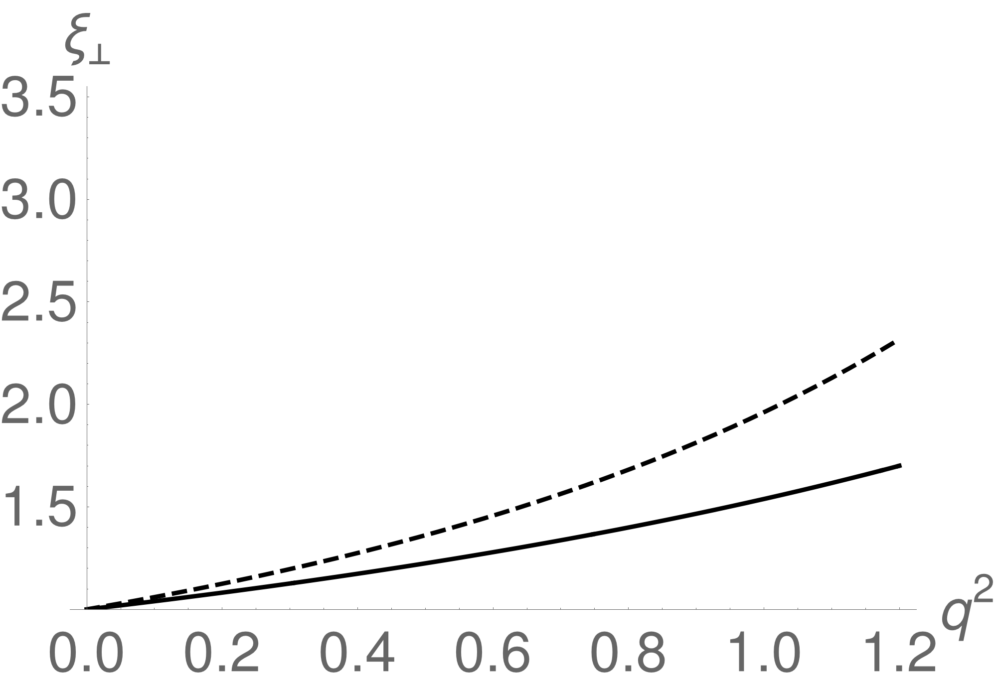
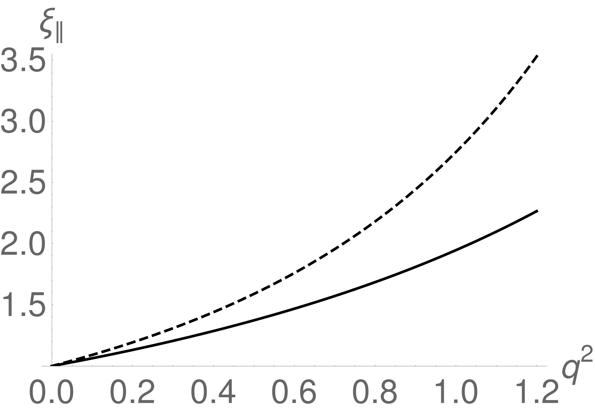
Figure 1: The dependence of the $D\to\rho$ transition form factors as a function of momentum transfer $q^{2}$ (in units of GeV², normalized to $q^{2}=0$), following from (23) [dashed line], compared to the parametrization determined in Fajfer:2005ug [solid line].

3.1.1 Corrections to the $D\to\rho$ form factors in the large recoil limit

Adapting the terminology of Beneke:2001at ; Beneke:2004dp , factorizable form-factor corrections are accounted for by Beneke:2004dp

$$C_{\perp}^{({\rm f},b)} =C_{7}^{\text{eff}}\Big{(}\ln\frac{m_{c}^{2}}{\mu^{2}}-L+\Delta M\Big{)}\,,\qquad C_{\parallel}^{({\rm f},b)}=-C_{7}^{\text{eff}}\Big{(}\ln\frac{m_{c}^{2}}{\mu^{2}}+2L+\Delta M\Big{)}\,;$$ (24)

whereas $C_{\perp,\parallel}^{({\rm f},d)}=0$. Here

$$L =-\frac{m_{c}^{2}-q^{2}}{q^{2}}\,\ln\left(1-\frac{q^{2}}{m_{c}^{2}}\right)\,,$$ (25)

and $\Delta M$ depends on the convention to define the charm-quark mass. In this work, we choose the $\overline{\rm MS}$ scheme for simplicity, which amounts to setting $\Delta M=0$. With our convention for defining the “soft” $D\to\rho$ form factors, the factorizable spectator corrections to the form factors are reflected in the contributions

$$T_{\perp,+}^{(\text{f},b)}=T_{\parallel,+}^{(\text{f},b)} =C_{7}^{\text{eff}}\,\frac{4m_{D}}{\bar{u}E}\,,$$ (26)

while $T_{a,-}^{(\text{f},b)}=0$ and $T_{a,\pm}^{(\text{f},d)}=0$ in the large-recoil limit.

3.2 Quark-loop topologies (w/o spectator effects)

Closing two quark lines from the 4-quark operators and radiating a (virtual) photon from the quark loop results in form-factor corrections to naive factorization that contribute to the effective Wilson coefficients in (15) as follows,

$$C_{\perp}^{(0,i)} =\delta^{ib}\,C_{7}^{\text{eff}}+\frac{q^{2}}{2m_{c}\,m_{D}}\,Y^{(i)}(q^{2})\,,\qquad C_{\parallel}^{(0,i)}=-\delta^{ib}\,C_{7}^{\text{eff}}-\frac{m_{D}}{2m_{c}}\,Y^{(i)}(q^{2})\,.$$ (27)

Here, the 1-loop functions $Y^{(i)}(s)$ can be decomposed as follows deBoer:2016dcg ,

$$Y^{(b)}(s) =\left[h(s,m_{c})+h(s,m_{u})\right]\Big{(}7\,C_{3}+\frac{4}{3}\,C_{4}+76\,C_{5}+\frac{64}{3}\,C_{6}\Big{)}$$ (28)

$$\quad{}-h(s,m_{s})\Big{(}\frac{2}{3}\,C_{1}+\frac{1}{2}\,C_{2}+3\,C_{3}+30\,C_{5}\Big{)}$$ (29)

$$\quad{}-h(s,m_{d})\Big{(}3\,C_{3}+30\,C_{5}\Big{)}+\frac{8}{9}\left(3\,C_{3}+16\,C_{5}+\frac{16}{3}\,C_{6}\right)\,,$$ (30)

and

$$Y^{(d)}(s) =-\Big{(}\frac{2}{3}\,C_{1}+\frac{1}{2}\,C_{2}\Big{)}[h(s,m_{s})-h(s,m_{d})]\,,$$ (31)

where the function $h(s,m)$ can be found, for instance, in Buchalla:1995vs , and – with our normalization convention – is given in (87) in the appendix. Notice that the contribution of the function $Y^{(b)}(s)$ to the decay amplitudes is strongly CKM suppressed. On the other hand, the function $Y^{(d)}(s)$ vanishes in the limit $m_{s}\to m_{u,d}\simeq 0$. Furthermore, at scales of the order of the charm-quark mass one encounters numerical cancellations in the combination of Wilson coefficients $(4/3\,C_{1}+C_{2})$; the effect is illustrated in Fig. 2. In particular, one observes a large shift when going from the LL to the NLL result, indicating that this combination of Wilson coefficients is particularly affected by higher-order radiative corrections, see also the discussion around Fig. 4.

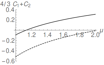
Figure 2: The combination of Wilson coefficients $(4/3\,C_{1}+C_{2})$ as a function of the renormalization scale $\mu$ (in units of GeV) at LL (dashed line) and NLL (solid line) accuracy.

At this point it is to be stressed that, strictly speaking, the perturbative calculation of the loop-function $h(s,m)$ is only justified in the deep Euclidean region, where $-s=Q^{2}\gg\Lambda_{\rm QCD}^{2}$. In contrast, for time-like momentum transfer, $s=q^{2}>0$, the $q^{2}$-dependence would rather be given by a hadronic spectral function that describes the effects of a tower of light vector mesons and multi-hadron final states with the appropriate quantum numbers. While in the corresponding $B$-meson decays, the annihilation topologies only provide a correction to the total decay amplitude, this is no longer the case for $D\to\rho\,\ell^{+}\ell^{-}$ decays, see also earlier estimates in Refs. Khodjamirian:1995uc ; Lyon:2012fk . In addition, for $B$-meson decays the region of small momentum transfer, $4m_{\ell}^{2}\leq q^{2}\lesssim\mbox{1-2~{}GeV${}^{2}$}$, could simply be excluded from the phenomenological analysis. Due to the restricted phase space this is no longer possible in $D$-meson decays. For this reason one should carefully discuss the associated parametric and systematic hadronic uncertainties. Inevitably, this requires some hadronic modelling. In particular, the amount of GIM cancellation in the difference $h(s,m_{s})-h(s,m_{d})$ in the perturbative calculation will be quite different from estimates based on hadronic models.

A straightforward approach, which has already been extensively used in the past Fajfer:2007dy ; Cappiello:2012vg ; Fajfer:2012nr ; Fajfer:2015mia ; deBoer:2017que , assumes that the long-distance hadronic effects are completely dominated by the lowest-lying narrow vector states ($\rho,\omega,\phi$ etc.) which are then modelled by Breit-Wigner resonances. In this work, we propose a more involved (but still oversimplified) picture, following Shifman:2000jv ; Shifman:2003de , where (i) a model for the infinite tower of higher resonances is included, and (ii) the shape of the Breit-Wigner resonances for the lowest states is modified to be in accordance with simple (leading-order) analyticity arguments. As explained in more detail in Appendix B, our idea amounts to replacing

$$h(q^{2},m_{q}) \to h(-\sigma^{2},m_{q})+\frac{4}{9}\,\int_{0}^{\infty}ds\,\frac{\sigma^{2}+q^{2}}{\sigma^{2}+s}\,\frac{j_{q}(s)}{s-q^{2}-i\epsilon}\,,\qquad(m=0,m_{s})$$ (32)

where the precise form of the spectral function $j_{q}(s)$, which models the effect of hadronic vector resonances with the corresponding quantum numbers, and the meaning of the parameter $\sigma^{2}$ can be found in Appendix B. In Fig 3 we illustrate the effect of the resonance model on the difference $[h(q^{2},m_{s})-h(q^{2},m_{d})]$ in the low-$q^{2}$ region, relevant for $D\to\rho$ decays. One observes that neither the sign nor the order of magnitude nor the shape of the hadronic model can be reproduced by the perturbative result (despite the fact that – by construction – for $q^{2}<0$ one has almost perfect numerical agreement, see Figs. 9,10 in the appendix).

It is important to note that the numerical effect of the vector resonances in rare semileptonic $D$-decays will be quite different from $B$-decays or $e^{+}e^{-}$ annihilation. While in the latter case, the cross section for $e^{+}e^{-}\to\text{hadrons}$ will be given by the imaginary part of the loop function, in $B$-decays the dominating correction to the decay width will arise from the interference with the short-distance terms (which do not yield strong phase differences), and therefore one will probe the real part of the loop function (see e.g. Beylich:2011aq ). In $D$-meson decays, however, the short-distance part is heavily suppressed, and therefore we expect the dominating effect to be given by the absolute value of the loop function, see Fig. 3.

 

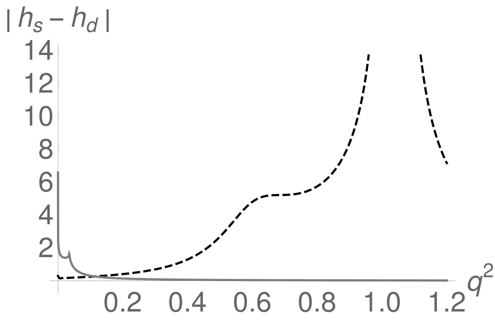
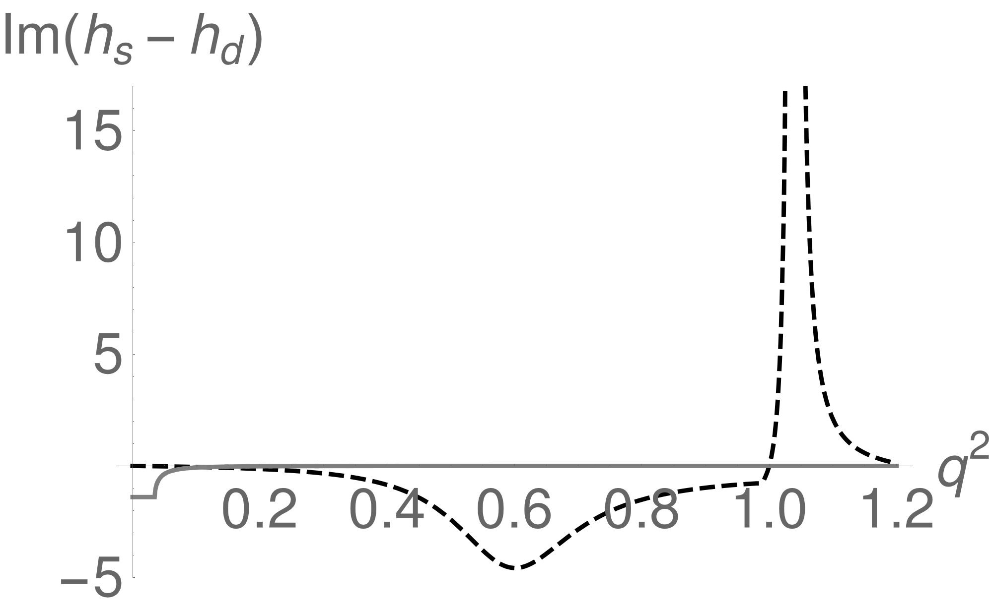
Figure 3: Comparison of the perturbative result for the absolute value and the imaginary part of the function $h(q^{2},m_{s})-h(q^{2},m_{d})$ (gray solid line) and the model (32) for its hadronic modification (black dashed line), as a function of momentum transfer $q^{2}$ (in units of GeV²). The parameter values are chosen as follows. For the modelling of the $d$-quark loop ($m_{d}=0$), we take $\sigma^{2}=2~{}\text{GeV}^{2}$, $a=1$, $b=1/6$. For the $s$-quark loop ($m_{s}=100$ MeV), we use $\sigma_{s}^{2}=2~{}\text{GeV}^{2}$, $a_{s}=1.4$, $b_{s}=0.1$. The parameters $n_{V}=1.94$ and $n_{\phi}=2.37$ are tuned to reproduce the perturbative result for $h(q^{2},m_{s/d})$ in the limit $q^{2}\to-\infty$. For details, see appendix B.

3.2.1 Non-factorizable $c\to u$ form-factor corrections

The remaining non-factorizable contributions can be expressed in terms of $q^{2}$-dependent short-distance functions $F_{i}^{(j)}$, which enter as follows (see Beneke:2001at ; Beneke:2004dp )

$$C_{F}C_{\perp}^{({\rm nf},i)} =-\Big{(}-C_{1}(F_{1}^{(7)}-\delta_{id}F_{1,d}^{(7)})-C_{2}(F_{2}^{(7)}-\delta_{id}F_{2,d}^{(7)})+\delta_{ib}C_{8}^{\text{eff}}F_{8}^{(7)}$$

$$-\frac{q^{2}}{2m_{c}m_{D}}\Big{[}C_{1}(F_{1}^{(9)}-\delta_{id}F_{1,d}^{(9)})+C_{2}(F_{2}^{(9)}-\delta_{id}F_{2,d}^{(9)})-\delta_{ib}C_{8}^{\text{eff}}F_{8}^{(9)}\Big{]}\Big{)}\,,$$

$$C_{F}C_{\parallel}^{({\rm nf},i)} =-\Big{(}C_{1}(F_{1}^{(7)}-\delta_{id}F_{1,d}^{(7)})+C_{2}(F_{2}^{(7)}-\delta_{id}F_{2,d}^{(7)})-\delta_{ib}C_{8}^{\text{eff}}F_{8}^{(7)}$$

$$+\frac{m_{D}}{2m_{c}}\Big{[}C_{1}(F_{1}^{(9)}-\delta_{id}F_{1,d}^{(9)})+C_{2}(F_{2}^{(9)}-\delta_{id}F_{2,d}^{(9)})-\delta_{ib}C_{8}^{\text{eff}}F_{8}^{(9)}\Big{]}\Big{)}\,.$$ (33)

At this point, a few comments are in order on how to obtain the functions $F_{i}^{(j)}$ from the expressions which have been calculated for the corresponding $b\to(s,d)\gamma^{*}$ amplitudes:

• The functions $F_{8}^{(7)}$ and $F_{8}^{(9)}$ can be obtained by changing the corresponding charge factors (which amounts to multiplying by ${Q_{u}}/{Q_{d}}$, where $Q_{u,d}$ are the charge factors for up- and down-quarks, respectively).

• In order to get the functions $F_{1,d}^{(7)},F_{1,d}^{(9)},F_{2,d}^{(7)}$ and $F_{2,d}^{(9)}$, one has to go back to the bare (i.e. unrenormalized) functions from $b$-decays Seidel:2004jh , replace the charge factors and renormalize the functions. Here, the renormalization constant with general charge factors can be derived from the results given in Gambino:2003zm and reads

  $$Z =\frac{\alpha_{s}}{4\pi}\,\frac{1}{\epsilon}\,\setcounter{MaxMatrixCols}{12}\begin{pmatrix}-2&\frac{4}{3}&0&-\frac{1}{9}&0&0&0&0&-\frac{8Q_{u}}{9}&0&\frac{5}{12}&\frac{2}{9}\\[1.00006pt] 6&0&0&\frac{2}{3}&0&0&0&0&-\frac{2Q_{u}}{3}&0&1&0\end{pmatrix}$$

  $$+\Big{(}\frac{\alpha_{s}}{4\pi}\Big{)}^{2}\frac{1}{\epsilon}\,\setcounter{MaxMatrixCols}{12}\begin{pmatrix}0&0&0&0&0&0&\frac{4Q_{d}}{81}-\frac{Q_{u}}{3}&0&\frac{-44Q_{d}}{243}-\frac{2Q_{u}}{9}&0&0&0\\[1.00006pt] 0&0&0&0&0&0&\frac{-8Q_{d}}{27}+2Q_{u}&0&\frac{88Q_{d}}{81}+\frac{16Q_{u}}{3}&0&0&0\end{pmatrix}$$

  $$+\Big{(}\frac{\alpha_{s}}{4\pi}\Big{)}^{2}\frac{1}{\epsilon^{2}}\,\setcounter{MaxMatrixCols}{12}\begin{pmatrix}0&0&0&0&0&0&0&0&-\frac{4(-2Q_{d}+3(-69+4n_{f})Q_{u})}{81}&0&0&0\\[1.00006pt] 0&0&0&0&0&0&0&0&-\frac{2(8Q_{d}+3(-21+2n_{f})Q_{u})}{27}&0&0&0\end{pmatrix}.$$ (34)

• The results for the functions $F_{1}^{(7)},F_{1}^{(9)},F_{2}^{(7)}$ and $F_{2}^{(9)}$ with general charge factors have been reconstructed from Mathematica notebooks that have been kindly provided by Christoph Greub (related to the work in Greub:2008cy ).

• For the limit $q^{2}\to 0$, the relevant functions $F_{1}^{(7)}$ and $F_{2}^{(7)}$ can be directly extracted from Greub:1996tg .

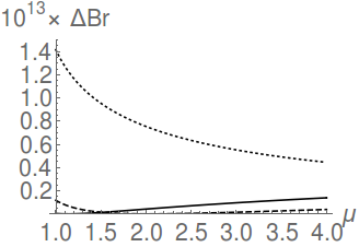
Figure 4: Contribution of quark-loop topologies to the differential branching ratio, integrated over a $q^{2}$-bin $[0.5,0.7]~{}{\rm GeV}^{2}$, as a function of the renormalization scale $\mu$ (in units of GeV), restricted to the contributions proportional to $\lambda_{d}$. The LO result with LL (NLL) Wilson coefficients is shown as the dashed (solid) line. The NLO contributions with NLL Wilson coefficients is shown as the dotted line.

As explained in Section 3.2, the leading contributions from quark-loop topologies in $D\to\rho$ transitions suffer from a renormalization-scale uncertainty due to partial numerical cancellations in the combination of Wilson coefficients $(\frac{4}{3}\,C_{1}+C_{2})$. The higher-order corrections encoded in (33) are expected to reduce this uncertainty. To numerically investigate the effect, we plot in Fig. 4 the contribution to the partially integrated branching ratio, $0.5~{}{\rm GeV}^{2}\leq q^{2}\leq 0.7~{}{\rm GeV}^{2}$, of the quark-loop topologies as a function of the renormalization scale $\mu$ (where we have restricted ourselves to the CKM-favoured contributions proportional to $\lambda_{d}$). We observe that the NLO corrections actually dominate over the LO contribution. On the one hand, this removes the issue with the accidental numerical cancellations at LO. On the other hand, it implies a very slow convergence of the perturbative series, i.e. large renormalization-scale uncertainties even at NLO. (We remind the reader that annihilation and spectator-scattering topologies will induce additional and formally independent scale uncertainties.)

3.3 Annihilation

As already mentioned, the so-called annihilation topologies will turn out to give large contributions to the decay rate, and therefore the associated hadronic uncertainties will be essential for phenomenological studies. The fact that the quark propagators in the annihilation diagrams involve time-like virtualities implies a particular sensitivity to the modelling of hadronic resonance effects. Furthermore, annihilation diagrams with the photon radiated from the quarks in the final-state meson are formally power-suppressed in the $1/m_{c}$ expansion, but may still be phenomenologically important. In particular, radiative corrections to these topologies have not been systematically computed in QCDF so far. As a consequence, the ambiguities related to the renormalization-scale setting in the relevant Wilson coefficients will remain a major source of theoretical uncertainties.

In the heavy-quark limit, the leading contributions from quark annihilation topologies originate from photon radiation off the light-quark in the $D$-meson. The results thus depends on the charge factor $e_{q}$ of the spectator quark. Translating the results from $b\to s,d$ to $c\to u$ transitions, we obtain

$$m_{c}\,T_{\parallel,-}^{(0,b)} =-e_{q}\,\frac{4m_{D}^{2}\,\omega}{m_{D}\,\omega-q^{2}-i\epsilon}\,(\delta_{qd}-\delta_{qu})\Big{[}C_{3}+\frac{4}{3}\Big{(}C_{4}+12\,C_{5}+16\,C_{6}\Big{)}\Big{]}\,,$$

$$m_{c}\,T_{\parallel,-}^{(0,d)} =e_{q}\,\frac{4m_{D}^{2}\,\omega}{m_{D}\,\omega-q^{2}-i\epsilon}\Big{[}\delta_{qd}\,3C_{2}+\delta_{qu}\Big{(}\frac{4}{3}\,C_{1}+C_{2}\Big{)}\Big{]}\,.$$ (35)

Again, the contributions from $T_{\parallel,-}^{(0,b)}$ will be strongly CKM suppressed. Therefore, for charged $D$-meson decays ($q=d$) the annihilation contribution is triggered by the Wilson coefficient $C_{2}$, while for neutral $D$-meson decays ($q=u$) it is proportional to the same combination $\frac{4C_{1}}{3}+C_{2}$ as appearing in the quark-loop topologies. As a consequence, we expect that charged $D$-meson decays will actually be dominated by annihilation topologies, since the partial numerical cancellation in Wilson coefficients does not occur here. In contrast, in neutral $D$-meson decays annihilation and quark-loop topologies will enter with similar magnitudes.

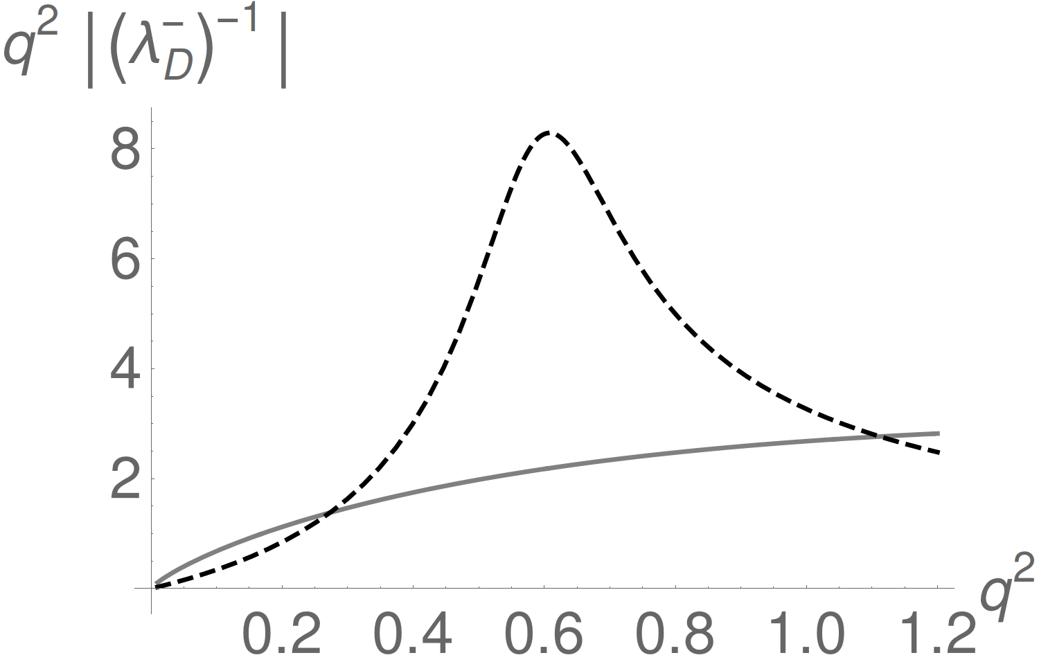
Figure 5: Comparison of the perturbative result for the absolute value of the function $\left(\lambda_{D}^{-}(q^{2})\right)^{-1}$ (massless spectator, gray solid line) and the model (37) for its hadronic modification (black dashed line). Notice that the result has been multiplied by $q^{2}$ (in units of GeV²). The parameter values are chosen as follows: $\sigma^{2}=2~{}\text{GeV}^{2}$, $a=1$, $b=1/6$. The $D$-meson LCDA is modelled by an exponential (38) with $\omega_{0}=0.45$ GeV. The parameter $n_{V}=2.40$ is tuned to reproduce the result for deep Euclidean values of $q^{2}$. For details, see appendix B.

The convolution of the expressions in (35) with the $D$-meson LCDA leads to the $q^{2}$-dependent “moment”

$$\left(\lambda_{D}^{-}(q^{2})\right)^{-1} =\int_{0}^{\infty}\frac{d\omega}{\omega-q^{2}/m_{D}-i\epsilon}\,\phi_{D}^{-}(\omega)\,,$$ (36)

whose analytic properties are further discussed in appendix B.2. Notice that the limit $q^{2}\to 0$ does not exist in (36) which limits the applicability of QCDF for that part of the amplitude to hard-collinear values of the momentum transfer that formally scale as $q^{2}\sim{\cal O}(\Lambda m_{D})\sim 1$ GeV². Moreover, as we have already discussed for the quark-loop contributions to the form-factor–like terms in the previous subsection, the physical $q^{2}$ spectrum in that region will be significantly influenced by light vector-meson resonances and looks quite different from the partonic result following from (36). Applying the same kind of model for the hadronic spectrum, as explained in appendix B.2, we end up with an estimate for the hadronic effects in $\lambda_{D}^{-}(q^{2})$. Here, the $q^{2}$-spectrum (given by the imaginary part of $(\lambda_{D}^{-})^{-1}$) is assumed to factorize into the $D$-meson LCDA and a hadronic model for the spectrum associated to the light vector current,

$$\left(\lambda_{D}^{-}(q^{2})\right)^{-1} \to\int_{0}^{\infty}\frac{ds}{s-q^{2}-i\epsilon}\,\phi_{D}^{-}(s/m_{D})\,j_{q}(s)\,.$$ (37)

The parameters in the function $j_{q}(s)$ are adjusted to reproduce the perturbative result in the limit $q^{2}\ll-m_{D}\,\Lambda$. To illustrate the numerical effect, we plot in Fig. 5 the absolute value of $\left[\lambda_{D}^{-}(q^{2})\right]^{-1}$ (the real and imaginary part are plotted in Fig. 11 in the appendix). Here we have taken a simple exponential model Grozin:1996pq ,

$$\phi_{D}^{-}(\omega) =\frac{1}{\omega_{0}}\,e^{-\omega/\omega_{0}}\,,\qquad\phi_{D}^{+}(\omega)=\frac{\omega}{\omega_{0}^{2}}\,e^{-\omega/\omega_{0}}\,,$$ (38)

for the LCDAs $\phi_{D}^{\pm}(\omega)$. The resulting picture looks quite similar as for the quark-loop functions $h(s,m)$. In particular the asymptotic behaviour for large values of $|q^{2}|$ is unchanged (by construction), while the typical modifications from the resonances occur in the region below $5$ GeV².

3.3.1 Power corrections of order $1/m_{D}$

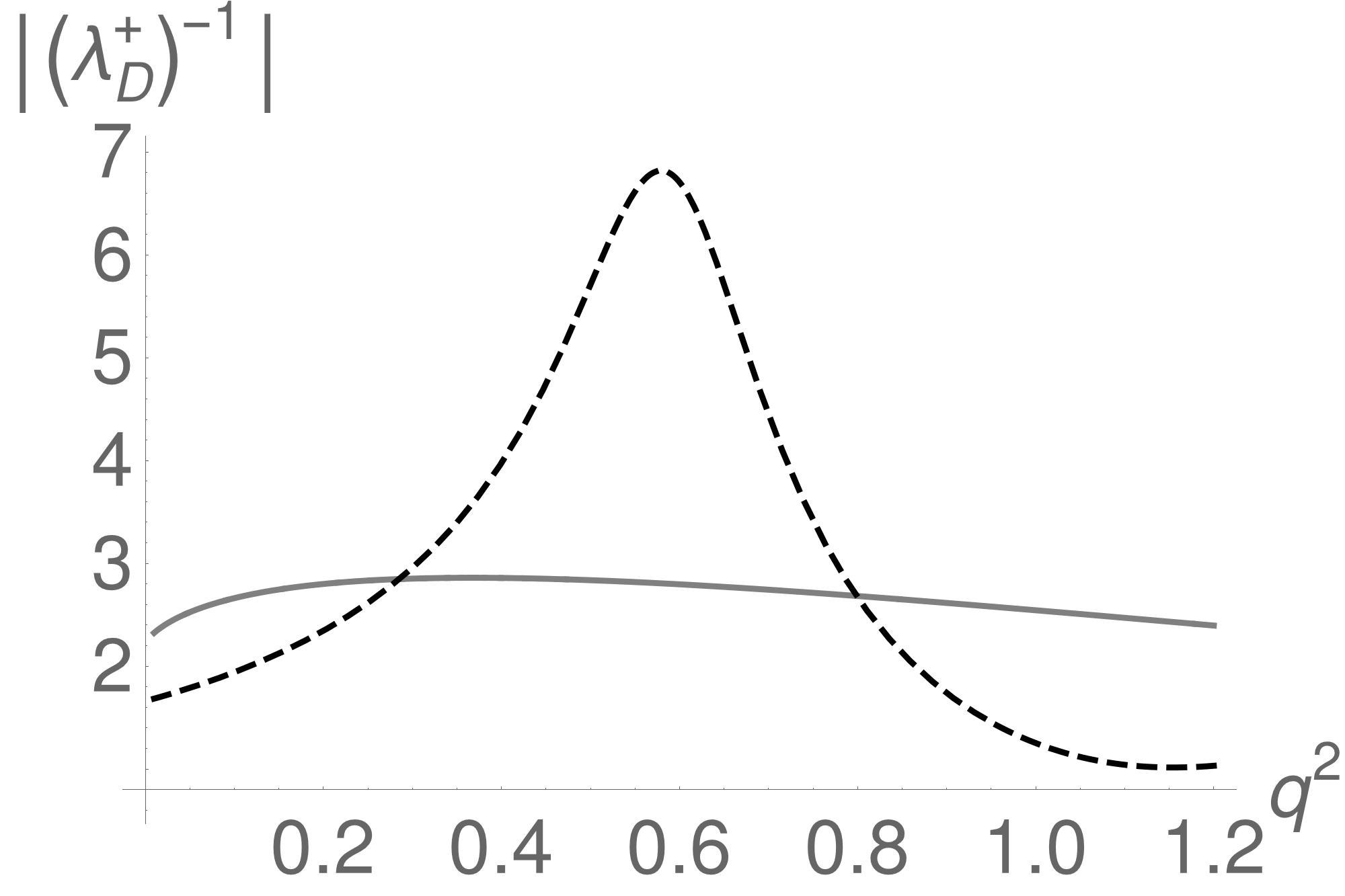
Figure 6: Comparison of the perturbative result for the absolute value of the function $\left(\lambda_{D}^{+}(q^{2})\right)^{-1}$ (massless spectator, gray solid line) and the model (42) for its hadronic modification (black dashed line). The parameter values are chosen as follows: $\sigma^{2}=2~{}\text{GeV}^{2}$, $a=1$, $b=1/6$. The $D$-meson LCDA is modelled by an exponential with $\omega_{0}=0.45$ GeV. The parameter $n_{V}=1.75$ is tuned to reproduce the result for deep Euclidean values of $q^{2}$. For details, see appendix B.

The contribution of annihilation topologies to the amplitudes for transversely polarized vector mesons only start at relative order $1/m_{D}$. It is known from the analysis of the analogous $B$-meson decays that these terms should not be neglected, in particular for observables that are sensitive to the transverse decay amplitudes or isospin asymmetries Bosch:2001gv ; Ali:2001ez ; Kagan:2001zk ; Feldmann:2002iw ; Beneke:2004dp . Translating again the known results from the $B$-meson sector, we end up with the following expressions,

$$m_{c}\,T_{\perp,+}^{(0,b)} =-e_{q}\,\frac{4\omega}{\bar{u}+us/m_{D}^{2}}(\delta_{qd}-\delta_{qu})\Big{[}C_{3}+\frac{4}{3}\Big{(}C_{4}+3C_{5}+4C_{6}\Big{)}\Big{]}$$ (39)

$$\quad+e_{q}\,\frac{2f_{\parallel}}{f_{\perp}}\frac{M_{V}}{1-s/m_{D}^{2}}\frac{m_{D}\omega}{m_{D}\omega-s-i\epsilon}(\delta_{qd}-\delta_{qu})\Big{[}C_{3}+\frac{4}{3}\Big{(}C_{4}+12C_{5}+16C_{6}\Big{)}\Big{]}\,,$$

$$m_{c}\,T_{\perp,+}^{(0,d)} =-e_{q}\,\frac{2f_{\parallel}}{f_{\perp}}\frac{M_{V}}{1-s/m_{D}^{2}}\frac{m_{D}\omega}{m_{D}\omega-s-i\epsilon}\Big{[}\delta_{qd}3C_{2}+\delta_{qu}\Big{(}\frac{4}{3}C_{1}+C_{2}\Big{)}\Big{]}\,.$$ (40)

Here, the first term arises from photon radiation off the constituents of the $\rho$-meson and therefore contains a non-trivial convolution with respect to the corresponding momentum fractions $u$ and $\bar{u}=1-u$. The other terms stem from sub-leading contributions from photon radiation off the $D$-meson constituents, which now give rise to the $q^{2}$-dependent “moment”

$$\left(\lambda_{D}^{+}(q^{2})\right)^{-1} =\int_{0}^{\infty}\frac{d\omega}{\omega-q^{2}/m_{D}-i\epsilon}\,\phi_{D}^{+}(\omega)\,.$$ (41)

As before, our hadronic model for the vector resonances can be implemented by the replacement

$$\left(\lambda_{D}^{+}(q^{2})\right)^{-1} \to\int_{0}^{\infty}\frac{ds}{s-q^{2}-i\epsilon}\,\phi_{D}^{+}(s/m_{D})\,j_{q}(s)\,.$$ (42)

The numerical effect is illustrated in Fig. 6 (see also Fig. 12 in the appendix). Notice that at $q^{2}=0$ the function $\lambda_{D}^{+}(0)$ describes the “soft” contribution to the $D\to\gamma$ transition form factor. The hadronic effects in our simple-minded model lead to a reduction of the form factor by $20-30$% which is in qualitative agreement with the findings in Braun:2012kp for the $B\to\gamma$ form factor.

3.4 Non-factorizable spectator scattering

Non-factorizable spectator scattering effects arise from matrix elements of the hadronic operators ${\cal O}_{1-6,8}$ where the (would-be) spectators in the $D\to\rho$ transitions take part in the short-distance scattering process. The various contributions that appear to order $\alpha_{s}$, again, can be adapted from Beneke:2001at ; Beneke:2004dp with the appropriate modifications for $c\to u$ transitions. We find

$$T_{\perp,+}^{(\text{nf},b)} =-\frac{4Q_{u}C_{8}^{\text{eff}}}{u+\bar{u}s/m_{D}^{2}}$$ (43)

$$\quad{}+\frac{m_{D}}{2m_{c}}\Bigg{[}Q_{u}\big{(}t_{\perp}(u,m_{c})+t_{\perp}(u,m_{u})\big{)}\left(C_{3}-\frac{1}{6}\,C_{4}+16\,C_{5}+\frac{10}{3}\,C_{6}\right)$$ (44)

$$\qquad\phantom{\frac{m_{D}}{2m_{c}}\Bigg{[}}{}-Q_{u}\,t_{\perp}(u,m_{c})\,\frac{4m_{c}}{m_{D}}\Big{(}C_{3}-\frac{1}{6}\,C_{4}+4\,C_{5}-\frac{2}{3}\,C_{6}\Big{)}$$ (45)

$$\qquad\phantom{\frac{m_{D}}{2m_{c}}\Bigg{[}}{}+Q_{d}\,t_{\perp}(u,m_{s})\left(C_{2}-\frac{1}{6}\,C_{1}+6\,C_{6}\right)+Q_{d}\,t_{\perp}(u,m_{d})\,6\,C_{6}\Bigg{]}\,,$$ (46)

and

$$T_{\parallel,+}^{(\text{nf},b)} =\frac{m_{D}}{m_{c}}\Bigg{[}Q_{u}\big{(}t_{\parallel}(u,m_{c})+t_{\parallel}(u,m_{u})\big{)}\left(C_{3}-\frac{1}{6}\,C_{4}+16\,C_{5}+\frac{10}{3}\,C_{6}\right)$$ (47)

$$\quad\phantom{\frac{m_{D}}{m_{c}}\Bigg{[}}+Q_{d}\,t_{\parallel}(u,m_{s})\left(C_{2}-\frac{1}{6}\,C_{1}+6\,C_{6}\right)+Q_{d}\,t_{\parallel}(u,m_{d})\,6\,C_{6}\Big{)}\Bigg{]}\,,$$ (48)

together with

$$T_{\perp,+}^{(\text{nf},d)} =Q_{d}\,\frac{m_{D}}{2m_{c}}\left(C_{2}-\frac{1}{6}\,C_{1}\right)\big{(}t_{\perp}(u,m_{s})-t_{\perp}(u,m_{d})\big{)}\,,$$ (49)

$$T_{\parallel,+}^{(\text{nf},d)} =Q_{d}\,\frac{m_{D}}{m_{c}}\left(C_{2}-\frac{1}{6}\,C_{1}\right)\big{(}t_{\parallel}(u,m_{s})-t_{\parallel}(u,m_{d})\big{)}\,,$$ (50)

and

$$T_{\parallel,-}^{(\text{nf},i)} =e_{q}\,\frac{m_{D}\,\omega}{m_{D}\,\omega-s-i\epsilon}\left[\delta^{ib}\frac{8C_{8}^{\text{eff}}}{\bar{u}+us/m_{D}^{2}}+\frac{6m_{D}}{m_{c}}\,F_{V}^{(i)}(\bar{u}m_{D}^{2}+us)\right]\,.$$ (51)

Here the quark-loop functions describing the relevant sub-diagrams are given by

$$F_{V}^{(b)}(s) =\big{(}h(s,m_{c})+h(s,m_{u})\big{)}\left(C_{3}+\frac{5}{6}\,C_{4}+16\,C_{5}+\frac{22}{3}\,C_{6}\right)$$ (52)

$$\quad{}+h(s,m_{s})\left(C_{2}-\frac{1}{6}\,C_{1}+C_{4}+10\,C_{6}\right)$$ (53)

$$\quad{}+h(s,m_{d})\big{(}C_{4}+10\,C_{6}\big{)}+\frac{8}{9}\left(2\,C_{4}-\frac{16}{5}\,C_{5}+\frac{128}{15}\,C_{6}\right)\,,$$ (54)

$$F_{V}^{(d)}(s) =\left(C_{2}-\frac{1}{6}\,C_{1}\right)\big{(}h(s,m_{s})-h(s,m_{d})\big{)}\,,$$ (55)

while the functions $t_{\perp,\parallel}(u,m_{q})$ and the definition of $C_{8}^{\rm eff}$ can be found in Beneke:2001at .

Notice that the contribution to the CKM-favoured amplitudes for transversely polarized vector mesons, $T_{\perp,+}^{(nf),d}$ in (50), are again GIM-suppressed. We therefore also include power corrections of relative order $1/m_{D}$ to the transverse amplitudes, which again can be adapted from the corresponding expressions for $B$-meson decays. We find

$$T_{\perp,+}^{(0,i)} =4e_{q}\,\delta^{ib}\,C_{8}^{\text{eff}}\,\frac{\omega}{m_{D}}\Big{(}\frac{1}{\bar{u}+us/m_{D}^{2}}+\frac{1}{(\bar{u}+us/m_{D}^{2})^{2}}\Big{)}$$ (56)

$$\quad{}+6e_{q}\,\frac{\omega}{m_{c}(\bar{u}+us/m_{D}^{2})}\,F_{V}^{(i)}(\bar{u}m_{D}^{2}+us)$$ (57)

$$\quad{}-3e_{q}\,\frac{M_{V}}{m_{c}(1-s/m_{D}^{2})}\,\frac{f_{\parallel}}{f_{\perp}\phi_{\perp}(u)}\,\frac{m_{D}\,\omega}{m_{D}\,\omega-s-i\epsilon}\ F_{V}^{(i)}(\bar{u}m_{D}^{2}+us)\,\int_{0}^{u}dv\,\frac{\phi_{\parallel}(v)}{v}\,.$$ (58)

4 Numerical Results

In this section we present some numerical estimates following from our theoretical analysis in the previous section. The theoretical predictions for the differential decay rates depend on a number of parameters. The most important hadronic input parameters are listed in Table 2. The remaining input parameters that have been used for the numerical analysis are listed in Table 11 in the appendix for completeness. Here a comment is in order about our choice for the parameter $\omega_{0}$ which determines the average value for the light-cone momentum of the spectator quark in the $D$-meson. While the analogous parameter for $B$-meson decays has been studied in some detail in the past (see e.g. Beneke:2011nf ; Braun:2012kp and references therein), there is practically no theoretical or phenomenological information on the $D$-meson LCDAs. We have therefore used an ad-hoc range for $\omega_{0}$ which reflects the naive expectation from heavy-quark symmetry with a sufficiently conservative uncertainty.

$A_{1}(0)$	$0.56\pm 0.01^{+0.02}_{-0.03}$	CLEO:2011ab
$A_{2}(0)$	$0.47\pm 0.06^{+0.04}_{-0.04}$	CLEO:2011ab
$V(0)$	$0.84\pm 0.09^{+0.05}_{-0.06}$	CLEO:2011ab
$f_{\rho,\parallel}$	$209\pm 1$ MeV	PDG
$f_{\rho,\perp}(1\,\rm{GeV})$	$165\pm 9$ MeV	Ball:2006nr
$a_{2}(\rho)_{\perp,\parallel}$	$0.15\pm 0.07$	Ball:2006nr
$f_{D}$	$(209\pm 3)$ MeV	Vladikas:2015bra
$\omega_{0}$	$(450\pm 150$ MeV	(ad-hoc)

Table 2: Summary of the most relevant hadronic input parameters.

4.1 Detailed breakdown of contributions to ${\cal C}_{9,\perp}$ and ${\cal C}_{9,\parallel}$

We first summarize the individual contributions to the coefficient functions ${\cal C}_{9,\perp}(q^{2})$ and ${\cal C}_{9,\parallel}(q^{2})$ as defined in Eq. (15) at NLO, at a benchmark value $q^{2}=0.5$ GeV² for the momentum transfer, see Tables 3 and 4. Compared to the situation in the analogous $B$-meson decays (see the discussion in Beneke:2004dp ), one observes a number of important differences:

• As is well known, the purely short-distance contribution from the Wilson coefficient $C_{9}$ is heavily suppressed by two effects: (i) the GIM cancellation between down-type quarks running in the loops, leading to a factor-10 smaller value for $C_{9}$ in $D$-decays compared to $B$-decays; (ii) the CKM suppression for $c\to u$ transitions, reflected by $\lambda_{b}\ll\lambda_{d}$. The decay amplitudes are therefore dominated by long-distance contributions proportional to the CKM structure $\lambda_{d}$.

• Among these, it turns out that for the neutral decay mode – at least at the considered value of $q^{2}$ – non-factorizable form-factor corrections (FFnf) and annihilation topologies (Ann) enter with the same order of magnitude, and also non-factorizable spectator effects (Specnf) give a non-negligible contribution. In the case of transverse vector mesons this requires to include (numerically unsuppressed) power corrections to annihilation spectator topologies ($1/M$ Ann) as well.

• The charged decay modes are completely dominated by contributions from annihilation topologies, where again the case of transverse vector mesons requires to include terms that are formally suppressed by $1/M_{D}$.

• We stress again that in each case, the estimates for the relevant long-distance contributions within the QCDF approach are very sensitive to hadronic resonance effects which adds to the systematic theoretical uncertainties.

Decay	Contr.	$\propto\lambda_{b}$	$\propto\lambda_{d}$
$D^{0}\to\rho_{\perp}^{0}\ell^{+}\ell^{-}$	$C_{9}$	$-0.445$	$0$
	FFf	$0.186-0.252i$	$-0.006+0.000i$
	FFnf	$1.373+1.254i$	$0.071-0.044i$
	Specf	$0.071$	$0$
	Specnf	$-0.114+0.009i$	$-0.013+0.009i$
	$1/M$ Ann	$-0.191+0.209i$	$-0.271-0.372i$
	$1/M$ Spec	$0.243+0.082i$	$0.002-0.006i$
${\cal C}_{9,\perp}$	Sum	$1.123+1.302i$	$-0.217-0.413i$
$D^{0}\to\rho^{0}_{\parallel}\ell^{+}\ell^{-}$	$C_{9}$	$-0.445$	$0$
	FFf	$-0.106-0.252i$	$-0.006+0.000i$
	FFnf	$0.267+0.570i$	$0.029+0.020i$
	Ann	$-0.050+0.206i$	$0.088-0.366i$
	Specf	$-0.027$	$0$
	Specnf	$0.146+0.019i$	$-0.008+0.004i$
${\cal C}_{9,\parallel}$	Sum	$-0.215+0.543i$	$0.103-0.342i$

Table 3: Breakdown of individual contributions to coefficient functions ${\cal C}_{9,\perp}$ and ${\cal C}_{9,\parallel}$ at NLO for the neutral decay mode, $D^{0}\to\rho^{0}\ell^{+}\ell^{-}$ at $q^{2}=0.5$ GeV². The renormalization scale is set to $\mu=1.5$ GeV. All other input parameters are set to their default values. Here $C_{9}$ denotes the purely short-distance contribution. We further list factorizable (FFf) and non-factorizable (FFnf) form-factor corrections, annihilation (Ann) at leading power, factorizable (Specf) and non-factorizable (Specnf) spectator interactions at leading power, as well as the included power corrections ($1/M$) to annihilation and spectator topologies.

Decay	Contr.	$\propto\lambda_{b}$	$\propto\lambda_{d}$
$D^{+}\to\rho_{\perp}^{+}\ell^{+}\ell^{-}$	$C_{9}$	$-0.445$	$0$
	FFf	$0.187-0.252i$	$-0.006+0.000i$
	FFnf	$1.376+1.256i$	$0.071-0.044i$
	Specf	$0.071$	$0$
	Specnf	$-0.114+0.009i$	$-0.013+0.009i$
	$1/M$ Ann	$-0.095+0.104i$	$2.472+3.381i$
	$1/M$ Spec	$-0.121-0.041i$	$-0.001+0.003i$
${\cal C}_{9,\perp}$	Sum	$0.859+1.077i$	$2.523+3.349i$
$D^{+}\to\rho^{+}_{\parallel}\ell^{+}\ell^{-}$	$C_{9}$	$-0.445$	$0$
	FFf	$-0.106-0.252i$	$-0.006+0.000i$
	FFnf	$0.266+0.570i$	$0.029+0.020i$
	Ann	$-0.025+0.103i$	$-0.799+3.335i$
	Specf	$-0.027$	$0$
	Specnf	$-0.186+0.001i$	$-0.009+0.009i$
${\cal C}_{9,\parallel}$	Sum	$-0.523+0.422i$	$-0.785+3.364i$

Table 4: Same as Table 3 for the charged mode, $D^{+}\to\rho^{+}\ell^{+}\ell^{-}$.

4.2 Differential decay rates

We next turn to the differential decay rates, where we distinguish between the contributions of transverse and longitudinal $\rho$ mesons, $d\Gamma_{T,L}$, which are obtained by projection onto the terms with $(1\pm\cos^{2}\theta)$ in Eq. (18). In Figs. 7 and 8 we show our result for the differential branching fractions in the case of neutral and charged mesons, respectively. Here, we compare the LO and NLO results, displaying only the uncertainties from scale variation for simplicity. The following comments can be made:

• The difference between the central values for the LO and NLO predictions (for our default choice of $\mu$) is not very pronounced.

• Still, at least for the neutral decay mode, we observe a large renormalization-scale dependence. This can be traced back to the issues with the combination of Wilson coefficients $(4/3C_{1}+C_{2})$ (see the discussion around Fig. 2) appearing in the relevant annihilation contributions in (35) and (40). Such cancellations do not occur in the charged decay mode.

• One should be aware that (presently unknown) NLO corrections to annihilation are not included. This particularly concerns the charged decay modes which are completely dominated by annihilation topologies.

• The hadronic-resonance model mainly leads to an enhancement of the differential rates. This is related to the fact that the rates are sensitive to the absolute values of the modelled complex functions, which has already been pointed out above. As a consequence, in contrast to the well-known $R$-ratio, the pseudo-realistic $q^{2}$-spectrum does not show the naively expected oscillations around the perturbative result.

• There is, however, a small region around $q^{2}\simeq 0.75$ GeV², where the perturbative result does not seem to be very much affected by resonance effects, at least within our simplified hadronic model. However, in that region the differential branching fractions are small, and the relative uncertainties are large.

Apart from the renormalization-scale dependence, the main parametric uncertainties stem from the LCDA of the $D$-meson, while the modelling of the hadronic resonances yields an estimate for the systematic hadronic uncertainties. These are summarized in Tables 5–8, where we display our predictions for partially integrated branching ratios in specific $q^{2}$ bins. As one can see, the uncertainties in the chosen $q^{2}$ bins can easily exceed 100%. In addition, we also expect substantial contributions from higher orders in the $1/m_{D}$ expansion which, however, are difficult to quantify.

 

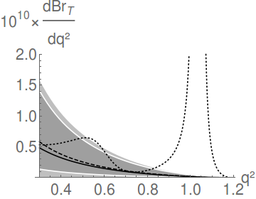
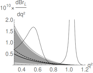
Figure 7: The differential branching ratios for $D^{0}\to\rho^{0}\ell^{+}\ell^{-}$ decays (in units of GeV^-2) with transversely or longitudinally polarized $\rho$ mesons as a function of momentum transfer $q^{2}$ (in GeV²). The LO QCDF result (including quark annihilation only at LO) is shown as the dashed line; the NLO result (without NLO corrections to annihilation) is shown as the solid line. The uncertainty bands (dark grey for LO; light grey for NLO) refer to the variation of the renormalization scale, only, with $\mu\in[1.3,2.0]~{}{\rm GeV}$. The dotted line illustrates the LO result for the hadronic resonance model.

$\Delta q^{2}$		Br${}_{\rm{T}}\times 10^{-12}$	$\mu$	$\omega_{0}$	hadr.
(0.3–0.5) GeV2	LO	$7.861$	${}^{+11.218}_{-7.833}$	${}^{+9.010}_{-3.428}$	$+3.574$
	NLO	$6.637$	${}^{+15.209}_{-4.726}$	${}^{+8.574}_{-3.149}$	$+1.752$
(0.5–0.7) GeV2	LO	$3.487$	${}^{+4.977}_{-3.475}$	${}^{+3.354}_{-1.437}$	$+4.713$
	NLO	$3.039$	${}^{+6.838}_{-2.153}$	${}^{+3.299}_{-1.367}$	$+3.820$
(0.7–0.9) GeV2	LO	$1.419$	${}^{+2.026}_{-1.414}$	${}^{+1.123}_{-0.547}$	$+1.450$
	NLO	$1.266$	${}^{+2.815}_{-0.893}$	${}^{+1.140}_{-0.536}$	$+0.865$

Table 5: Branching fractions for the neutral decay mode into transversely polarized vector mesons, partially integrated over different bins $\Delta q^{2}$.

$\Delta q^{2}$		Br${}_{\rm{L}}\times 10^{-12}$	$\mu$	$\omega_{0}$	hadr.
(0.3–0.5) GeV2	LO	$9.334$	${}^{+13.326}_{-9.302}$	${}^{+5.157}_{-2.756}$	$+11.300$
	NLO	$6.982$	${}^{+18.243}_{-5.418}$	${}^{+4.524}_{-2.321}$	$+8.759$
(0.5–0.7) GeV2	LO	$3.927$	${}^{+5.608}_{-3.914}$	${}^{+1.643}_{-1.026}$	$+19.766$
	NLO	$3.103$	${}^{+7.793}_{-2.360}$	${}^{+1.509}_{-0.903}$	$+16.051$
(0.7–0.9) GeV2	LO	$1.467$	${}^{+2.095}_{-1.462}$	${}^{+0.446}_{-0.334}$	$+0.198$
	NLO	$1.194$	${}^{+2.939}_{-0.899}$	${}^{+0.430}_{-0.304}$	$+0.115$

Table 6: Same as Table 5 for longitudinally polarized vector mesons.

 

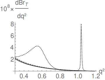
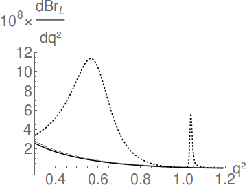
Figure 8: The same as Fig. 7 for $D^{+}\to\rho^{+}\ell^{+}\ell^{-}$ decays, with $\mu\in[1.0,2.0]~{}{\rm GeV}$.

$\Delta q^{2}$		Br${}_{\rm{T}}\times 10^{-9}$	$\mu$	$\omega_{0}$	hadr.
(0.3–0.5) GeV2	LO	$3.085$	${}^{+0.288}_{-0.123}$	${}^{+3.592}_{-1.360}$	$+2.763$
	NLO	$2.827$	${}^{+0.000}_{-0.000}$	${}^{+3.261}_{-1.237}$	$+2.937$
(0.5–0.7) GeV2	LO	$1.384$	${}^{+0.128}_{-0.054}$	${}^{+1.354}_{-0.577}$	$+4.836$
	NLO	$1.265$	${}^{+0.000}_{-0.000}$	${}^{+1.226}_{-0.523}$	$+5.417$
(0.7–0.9) GeV2	LO	$0.573$	${}^{+0.052}_{-0.022}$	${}^{+0.462}_{-0.224}$	$+0.030$
	NLO	$0.523$	${}^{+0.000}_{-0.000}$	${}^{+0.417}_{-0.202}$	$+0.350$

Table 7: Same as Table 5 for the charged decay mode.

$\Delta q^{2}$		Br${}_{\rm{L}}\times 10^{-9}$	$\mu$	$\omega_{0}$	hadr.
(0.3–0.5) GeV2	LO	$3.753$	${}^{+0.332}_{-0.140}$	${}^{+2.101}_{-1.120}$	$+7.365$
	NLO	$3.497$	${}^{+0.000}_{-0.000}$	${}^{+1.929}_{-1.032}$	$+7.523$
(0.5–0.7) GeV2	LO	$1.598$	${}^{+0.140}_{-0.059}$	${}^{+0.677}_{-0.421}$	$+16.022$
	NLO	$1.481$	${}^{+0.000}_{-0.000}$	${}^{+0.619}_{-0.387}$	$+17.028$
(0.7–0.9) GeV2	LO	$0.607$	${}^{+0.053}_{-0.022}$	${}^{+0.187}_{-0.139}$	$+1.959$
	NLO	$0.561$	${}^{+0.000}_{-0.000}$	${}^{+0.170}_{-0.127}$	$+2.703$

Table 8: Same as Table 6 for the charged decay mode.

4.3 Ratio of transverse and longitudinal rates

$\Delta q^{2}$		${\cal R}_{TL}$	$\mu$	$\omega_{0}$	hadr.
(0.3–0.5) GeV2	LO	$0.842$	${}^{+0.009}_{-0.000}$	${}^{+0.322}_{-0.168}$	$-0.288$
	NLO	$0.950$	${}^{+0.271}_{-0.363}$	${}^{+0.371}_{-0.202}$	$-0.417$
(0.5–0.7) GeV2	LO	$0.888$	${}^{+0.011}_{-0.000}$	${}^{+0.340}_{-0.181}$	$-0.542$
	NLO	$0.979$	${}^{+0.330}_{-0.608}$	${}^{+0.395}_{-0.219}$	$-0.621$
(0.7–0.9) GeV2	LO	$0.968$	${}^{+0.012}_{-0.000}$	${}^{+0.361}_{-0.198}$	$+0.755$
	NLO	$1.060$	${}^{+0.789}_{-0.726}$	${}^{+0.421}_{-0.240}$	$+0.568$

Table 9: Ratio of transverse and longitudinal rate as defined in Eq. (60) for the neutral decay mode.

$\Delta q^{2}$		${\cal R}_{TL}$	$\mu$	$\omega_{0}$	had
(0.3–0.5) GeV2	LO	$0.822$	${}^{+0.004}_{-0.002}$	${}^{+0.319}_{-0.167}$	$-0.296$
	NLO	$0.808$	${}^{+0.003}_{-0.009}$	${}^{+0.314}_{-0.163}$	$-0.285$
(0.5–0.7) GeV2	LO	$0.866$	${}^{+0.004}_{-0.002}$	${}^{+0.338}_{-0.180}$	$-0.513$
	NLO	$0.854$	${}^{+0.003}_{-0.009}$	${}^{+0.332}_{-0.176}$	$-0.493$
(0.7–0.9) GeV2	LO	$0.944$	${}^{+0.004}_{-0.002}$	${}^{+0.359}_{-0.197}$	$-0.709$
	NLO	$0.932$	${}^{+0.003}_{-0.009}$	${}^{+0.353}_{-0.193}$	$-0.665$

Table 10: Ratio of transverse and longitudinal rate as defined in Eq. (60) for the charged decay mode.

Given the large parametric and systematic uncertainties, we do not expect to obtain reasonably reliable predictions for the $D\to\rho\,\ell^{+}\ell^{-}$ differential decay rates within the QCDF framework. We will therefore briefly investigate to what extent at least some of the theoretical uncertainties might be reduced in ratios of decay widths. To this end we consider the ratio of partially integrated rates for transversely and longitudinally polarized vector mesons,

$${\cal R}_{TL} :=\left(\,\int\limits_{\Delta q^{2}}dq^{2}\,\frac{d\Gamma_{T}}{dq^{2}}\right)/\left(\,\int\limits_{\Delta q^{2}}dq^{2}\,\frac{d\Gamma_{L}}{dq^{2}}\right)\,.$$ (60)

In a generic NP scenario with sizeable short-distance contributions this ratio would be sensitive to the following combinations of Wilson coefficients in the large-recoil limit (see e.g. the discussion in Kruger:2005ep ),

$$\frac{{|C_{10}|}^{2}+{|C_{10}^{\prime}|}^{2}+{|C_{9}|}^{2}+{|C_{9}^{\prime}|}^{2}+\frac{4{\hat{m}_{c}}^{2}}{\hat{s}^{2}}\left({|C_{7}|}^{2}+{|C_{7}^{\prime}|}^{2}\right)+\frac{4{\hat{m}_{c}}}{\hat{s}}\,\text{Re}\left[{C_{7}}{C_{9}^{*}}+{C_{7}^{\prime}}{C_{9}^{\prime}{}^{*}}\right]}{|{C_{10}}-{C_{10}^{\prime}}|^{2}+|{C_{9}}-{C_{9}^{\prime}}|^{2}+\frac{4{\hat{m}_{c}}^{2}}{\hat{s}^{2}}\,|{C_{7}}-{C_{7}^{\prime}}|^{2}+\frac{4{\hat{m}_{c}}}{\hat{s}^{2}}\,\text{Re}\left[({C_{7}}-{C_{7}^{\prime}})({C_{9}}-{C_{9}^{\prime}})^{*}\right]}\,,$$

where the primed coefficients refer to the operators with flipped quark chiralities, $\hat{m}_{c}=m_{c}/M_{D}$, $\hat{s}=q^{2}/M_{D}^{2}$, and possible contributions from scalar or tensor operators have been neglected. We present estimates for the quantity ${\cal R}_{TL}$ in specific regions of momentum transfer $\Delta q^{2}$ in Tables 9 and 10. We observe that, indeed, the parametric and systematic uncertainties are somewhat reduced, at least for the lower two $q^{2}$ bins:

• For the neutral decay modes the scale dependence at NLO still can reach several 10 percent.

• The uncertainties induced by the parameter $\omega_{0}$ in the $D$-meson LCDA typically reaches up to 30%. Notice that this estimate has been obtained using a particular (simple) model function (38) for the two 2-particle $D$-meson LCDAs.

• As our model correlates the hadronic-resonance effects in the different decay topologies, we also found a slight reduction of the associated uncertainty in ${\cal R}_{TL}$. We emphasize again that the hadronic model is only meant for illustration, and therefore one should not draw specific conclusions about the resonance effects from this.

We have also investigated to what extent hadronic uncertainties may cancel in the leptonic forward-backward asymmetry. Normalizing to the transverse rate, depending on the relative phase of a possible NP contribution to the Wilson coefficient $C_{10}$, this observable is determined by the ratio ${\rm Re}\left[{\cal C}_{9,\perp}(q^{2})\,C_{10}^{*}\right]/|{\cal C}_{9,\perp}^{2}(q^{2})|$. As the real or imaginary part of the resonant contributions to ${\cal C}_{9,\perp}$ look rather different from the square of the absolute value, we did not observe a significant reduction of the associated theoretical uncertainties in that case.

5 Conclusions

In this paper we have investigated the rare semileptonic decays $D\to\rho\,\ell^{+}\ell^{-}$ in the framework of QCD factorization (QCDF). Here, our primary goal was not to obtain very precise predictions for the SM decay rates, but rather to achieve a sufficiently realistic (i.e. conservative) estimate of hadronic uncertainties related to long-distance QCD effects.

The QCDF framework allows one to separate contributions from various decay topologies via a simultaneous expansion in the strong coupling constant and inverse powers of the heavy charm-quark mass. This includes factorizable and non-factorizable effects from quark loops, annihilation topologies, as well as spectator-scattering effects. Within the perturbative analysis, we have found that in general the contributions from non-factorizable effects dominate. In the case of neutral mesons form-factor corrections, annihilation and spectator effects enter with similar magnitude, whereas the decay modes with charged mesons are dominated by annihilation topologies alone.

We have also seen that – not surprisingly – the convergence of the QCDF predictions for the considered decay rates is relatively poor, which is clearly to be attributed to the relatively small charm-quark mass, but also – in the case of neutral mesons – due to accidental cancellations between the Wilson coefficients multiplying the dominant expressions. Even more importantly, the restricted phase space for $D\to\rho$ transitions together with the suppression of the purely short-distance effects (i.e. the ones encoded in the semileptonic and electromagnetic operators) in the Standard Model imply a much stronger sensitivity to hadronic-resonance effects as compared to the analogous $B$-meson decays. In order to get a quantitative estimate of these effects, we have extended a model, that has been originally designed to describe the effect of vector resonances in $e^{+}e^{-}$ annihilation or hadronic $\tau$ decays. This allows us to study aspects of quark-hadron duality within the QCDF approach via dispersion relations and to estimate the related systematic uncertainties in the $q^{2}$ spectrum. (We repeat that we do not claim a realistic description of the $q^{2}$-spectrum itself.)

Together with the remaining parametric uncertainties coming from non-factorizable contributions and (yet unknown) higher-order effects in the QCDF approach (notably NLO corrections to the annihilation topologies), we have found that reliable theoretical predictions for the differential decay widths in $D\to\rho\,\ell^{+}\ell^{-}$ within the QCDF approach are almost impossible. On the other hand, part of the systematic and parametric uncertainties tend to partially cancel in ratios of decay widths, at least in certain regions of phase space. As an example, we have studied the ratio of transverse and longitudinal decay rates. Still, our conclusion about possible new-physics sensitivity of rare semileptonic $D$-meson decays tends to be somewhat pessimistic, unless one concentrates on bins in the lepton invariant mass far below (or, in case of radiative $D\to\pi\ell^{+}\ell^{-}$ decays, also far above) the light resonances, or one considers observables that (practically) vanish in the Standard Model. In this way one can still look for new-physics scenarios with large Wilson coefficients which are not excluded by current exprerimental data, see e.g. the discussion in the recent literature Fajfer:2015mia ; deBoer:2015boa . (To a certain extent, this also applies to the purely radiative decays $D\to\rho\gamma$ which have recently been seen by the Belle experiment Abdesselam:2016yvr .)

On the other hand, one may exploit the fact that non-factorizable hadronic effects are more pronounced in $D$-meson decays, and use $D\to\rho\,\ell^{+}\ell^{-}$ as a playground for QCD studies that are also relevant to estimate sub-leading effects in the corresponding $B$-meson decays.

Appendix A Explicit Formulas for $D\to\pi\ell^{+}\ell^{-}$ Decays

Defining generalized form factors for $D\to\pi\gamma^{*}$ transitions as

$$\langle\gamma^{*}(q,\mu)\,\pi^{+}(p^{\prime})|\mathcal{H}_{\rm eff}^{(i)}|D^{+}(p)\rangle =\frac{g_{\rm em}m_{c}}{4\pi^{2}}\,\frac{{\cal T}_{P=\pi}^{(i)}(q^{2})}{m_{D}}\,\left[q^{2}\,(p^{\mu}+p^{\prime\mu})-(m_{D}^{2}-M_{\pi}^{2})\,q^{\mu}\right]\,,$$ (61)

following Beneke:2001at , we obtain the factorization formula

$$\mathcal{T}_{P}^{(i)} \simeq-\xi_{P}\,C_{\parallel}^{(i)}+\frac{\pi^{2}}{N_{c}}\,\frac{f_{D}f_{P}}{m_{D}}\,\sum_{\pm}\int\frac{d\omega}{\omega}\,\phi_{D,\pm}(\omega)\,\int_{0}^{1}du\,\phi_{P}(u)\,T_{\parallel,\pm}^{(i)}(u,\omega)\,,$$ (62)

where the same functions $T_{\parallel,\pm}^{(i)}$ appear as in the case of decays into longitudinally polarized vector mesons, and $\xi_{P}(q^{2})$ is the soft form factor for $D\to\pi$ transitions as defined in Beneke:2001at . If we define again the coefficient function

$$\mathcal{C}^{(i)}_{9,P}(q^{2}) =\delta^{ib}\,C_{9}+\frac{2m_{c}}{m_{D}}\frac{\mathcal{T}_{P}^{(i)}(q^{2})}{\xi_{P}(q^{2})}\,,$$ (63)

the twofold differential decay rate can be written as

$$\frac{d^{2}\Gamma(D\to\pi\ell^{+}\ell^{-})}{dq^{2}d\rm{cos}\theta} =\frac{G_{F}^{2}}{128\pi^{3}}\,m_{D}^{3}\,S\,\lambda_{D}^{3}(q^{2},M_{\pi}^{2})\,\left(\frac{\alpha_{\rm{em}}}{4\pi}\right)^{2}\times$$ (64)

$$(1-\rm{cos}^{2}\theta)\,\xi_{\pi}^{2}(q^{2})\left|\lambda_{d}\,\mathcal{C}_{9,\pi}^{(d)}+\lambda_{b}\,\mathcal{C}_{9,\pi}^{(b)}\right|^{2}\,.$$ (65)

Appendix B Semi-naive Model for Duality violation

In the perturbative analysis of non-factorizing effects from hadronic operators, the virtual photon is treated as a point-like particle. However, at time-like virtualities, $q^{2}>0$, the coupling of the photon to a (perturbative) sum of intermediate partonic states has to be replaced by the coupling to an (infinite) sum over physical hadronic states. Parton-hadron duality (PHD) is expected to hold if one averages over a “sufficiently” large phase-space region of $q^{2}$. In order to estimate the numerical effect of violation of PHD, we will construct a simple model which reflects the main theoretical features and phenomenological constraints, following the ideas discussed in Blok:1997hs ; Shifman:2000jv ; Shifman:2003de (see also Cata:2005zj ; Cata:2008ye ; Cata:2008ru ; Boito:2011qt ; Beylich:2011aq ).

Preliminaries: (a) Modelling of vector resonances

The standard procedure to model a vector-meson resonance is to consider a Breit-Wigner (BW) ansatz,

$$f_{\rm BW}(q^{2}) =\frac{n_{V}\,M_{V}^{2}}{M_{V}^{2}-q^{2}-i\,M_{V}\Gamma_{V}}\,,\qquad\frac{1}{\pi}\,{\rm Im}\left[f_{\rm BV}\right]=\frac{n_{V}}{\pi}\,\frac{M_{V}^{3}\Gamma_{V}}{(q^{2}-M_{V}^{2})^{2}+M_{V}^{2}\,\Gamma_{V}^{2}}\,.$$ (66)

In the narrow-width approximation, one would further neglect $\Gamma_{V}/M_{V}\ll 1$. The above form gives a successful description of the resonance shape in the vicinity of $q^{2}\simeq M_{V}^{2}$; however, for our purposes we would also need to control the effect away from the resonance peak. A more sophisticated ansatz for a modified BW-like shape has been suggested by Shifman Shifman:2000jv ; Shifman:2003de , where

$$f_{\rm mod}(q^{2}) =\hat{n}_{V}\left(1+z_{V}\,\frac{\sigma_{V}^{2}}{M_{V}^{2}}\right)^{-1},\quad z_{V}=\left(\frac{-q^{2}-i\epsilon}{\sigma_{V}^{2}}\right)^{1-b_{V}/\pi},\quad b_{V}=\frac{\Gamma_{V}}{M_{V}}\,.$$ (67)

Among others, this form has the correct analytic behaviour, i.e. a branch cut at $q^{2}=0$ (we neglect the pion mass in the following). On the other hand, it reproduces the BW-ansatz when $q^{2}\simeq M_{V}^{2}\approx\sigma_{V}^{2}$ and $b_{V}\ll 1$. The imaginary part of the modified BW ansatz can then be approximated as ,

$$\frac{1}{\pi}\,{\rm Im}\left[f_{\rm mod}\right] =\frac{\hat{n}_{V}\,\theta(q^{2})}{\pi}\,\frac{|z_{V}|\,\hat{\sigma}_{V}^{2}\,\sin b_{V}}{1-2\,|z_{V}|\,\hat{\sigma}_{V}^{2}\,\cos b_{V}+|z_{V}|^{2}\,\hat{\sigma}_{V}^{4}}$$ (68)

$$\simeq\frac{n_{V}\,\theta(q^{2})}{\pi}\,\frac{q^{2}M_{V}\Gamma_{V}}{(q^{2}-M_{V}^{2})^{2}+q^{2}\,\Gamma_{V}^{2}}\,,$$ (69)

where in the last line we have taken $\hat{\sigma}_{V}^{2}=\sigma_{V}^{2}/M_{V}^{2}=1$ for simplicity and used $b_{V}\ll 1$.

For vector resonances in the $s\bar{s}$ channel, the definition of $z_{V}$ has to be modified to include the threshold for $K\bar{K}$ production. Neglecting mixing effects, this amounts to setting

$$f_{\rm mod}^{(s\bar{s})}(q^{2}) =\hat{n}_{V}\left(1+\tilde{z}_{V}\,\frac{\tilde{\sigma}_{V}^{2}}{\tilde{M}_{V}^{2}}\right)^{-1}\,,$$ (70)

with

$$\tilde{z}_{V}=\left(\frac{4m_{K}^{2}-q^{2}-i\epsilon}{\tilde{\sigma}_{V}^{2}}\right)^{1-\tilde{b}_{V}/\pi},\quad\tilde{b}_{V}=\frac{\tilde{\Gamma}_{V}}{\tilde{M}_{V}}\left(1-\frac{4m_{K}^{2}}{\tilde{\sigma}_{V}^{2}}\right)\,.$$ (71)

The imaginary part of the modified BW ansatz now reads (for $\tilde{\sigma}_{V}^{2}\simeq M_{V}^{2}$)

$$\frac{1}{\pi}\,{\rm Im}\left[f_{\rm mod}^{(s\bar{s})}\right] \simeq\frac{n_{V}}{\pi}\,\frac{(q^{2}-4m_{K}^{2})\,\theta(q^{2}-4m_{K}^{2})}{\tilde{M}_{V}^{2}-4m_{K}^{2}}\,\frac{q^{2}\tilde{M}_{V}^{3}\tilde{\Gamma}_{V}}{(q^{2}-\tilde{M}_{V}^{2})^{2}+\frac{q^{2}-4m_{K}^{2}}{\tilde{M}_{V}^{2}-4m_{K}^{2}}\,\tilde{M}_{V}^{2}\,\tilde{\Gamma}_{V}^{2}}\,.$$ (72)

Notice that in this form, the original BW ansatz is recovered in the limit $m_{K}^{2}\to-\infty$.

Preliminaries: (b) Resumming an infinite tower of vector resonances

Shifman Shifman:2000jv ; Shifman:2003de also gives a simple model to describe the effect of an infinite tower of equidistant vector resonances with masses $M_{n}^{2}=(n+a_{0})\,\sigma^{2}$ and widths $\Gamma_{n}=bM_{n}$, for $n=\{0,1,2,\ldots\}$ and $a_{0}={\rm const}$. To this end, one considers the function

$$\pi(q^{2}) =\frac{1}{1-b/\pi}\,\sum_{n=0}^{\infty}\frac{1}{n+a_{0}+z}=-\frac{1}{1-b/\pi}\,\Psi(z+a_{0})\,,\qquad z=\left(\frac{-q^{2}-i\epsilon}{\sigma^{2}}\right)^{1-b/\pi}\,.$$ (73)

Each individual resonance contributes with a modified BW term as discussed above. However, the infinite sum over all resonances reproduces the asymptotic result

$$\lim_{-q^{2}\to\infty}\pi(q^{2})=-\ln\frac{-q^{2}}{\sigma^{2}}+{\cal O}(\sigma^{2}/q^{2})\,.$$ (74)

In Shifman:2000jv ; Shifman:2003de , a simplified model has been constructed, taking $a_{0}=1$. In this case, one has

$$\psi(z+1)=\psi(z)+\frac{1}{z} =\psi(-z)-\pi\,\cot(\pi z)\,,$$ (75)

and for time-like momentum transfer, $q^{2}>0$, the imaginary part of $\pi(q^{2})$ receives an oscillatory contribution from the second term, with

$$\frac{1}{\pi}\,{\rm Im}\left[\pi(q^{2})\right]_{\rm osc.} \simeq{\rm Im}\left[\cot(\pi z)\right]$$ (76)

$$=-\frac{\sinh(2\pi|z|\sin b)\,\theta(q^{2})}{\cos(2\pi|z|\cos b)-\cosh(2\pi|z|\sin b)}$$ (77)

$$\approx\left(1+2\,\exp\left(-\frac{2\pi\,q^{2}\,b}{\sigma^{2}}\right)\cos\left(\frac{2\pi q^{2}}{\sigma^{2}}\right)\right)\theta(q^{2})\,,$$ (78)

where the last approximation is valid for $q^{2}>s_{0}\equiv\frac{\sigma^{2}}{2\pi\,b}$ (and $\frac{b}{\pi}\left|\ln\frac{q^{2}}{\sigma^{2}}\right|\ll 1$). The general idea is then to start from a perturbative result in the OPE/factorization approach, where the leading $q^{2}$ dependence is logarithmic, such that the spectrum is given by

$$j_{\rm OPE}(q^{2})=\theta(q^{2})+\ldots$$

and to replace it by the hadronic model (73) – which reproduces the oscillatory behaviour in (78) – and to add a finite number of vector resonances in the region $0<q^{2}<s_{0}$. In Shifman:2000jv ; Shifman:2003de a good fit to $\tau$ decay data in the vector channel has been obtained for $\sigma^{2}=2$ GeV² and $b=1/6$. (More sophisticated analyses with qualitatively similar parameter values can be found in Cata:2005zj ; Cata:2008ye ; Cata:2008ru ; Boito:2011qt ).

Our model ansatz for the hadronic spectrum with up/down or strange quarks in the loop therefore looks as follows.

$$j_{(u/d)}(q^{2}) =\frac{n_{V}}{\pi}\,\frac{q^{2}\,M_{V}\Gamma_{V}}{(q^{2}-M_{V}^{2})^{2}+q^{2}\,\Gamma_{V}^{2}}$$ (79)

$$\quad{}-\frac{1}{\pi}\,{\rm Im}\left[\frac{1}{1-b/\pi}\,\Psi(z+a)\right]\,,\qquad z=\left(\frac{-q^{2}-i\epsilon}{\sigma^{2}}\right)^{1-b/\pi}\,,$$ (80)

and

$$j_{(s)}(q^{2}) =\frac{n_{\phi}}{\pi}\,\frac{(q^{2}-4m_{K}^{2})\,\theta(q^{2}-4m_{K}^{2})}{m_{\phi}^{2}-4m_{K}^{2}}\,\frac{m_{\phi}^{3}\Gamma_{\phi}}{(q^{2}-m_{\phi}^{2})^{2}+\frac{q^{2}-4m_{K}^{2}}{m_{\phi}^{2}-4m_{K}^{2}}\,m_{\phi}^{2}\,\Gamma_{\phi}^{2}}$$ (81)

$$\quad{}-\frac{1}{\pi}\,{\rm Im}\left[\frac{1}{1-b_{s}/\pi}\,\Psi(z_{s}+a_{s})\right]\,,\qquad z_{s}=\left(\frac{4m_{K}^{2}-q^{2}-i\epsilon}{\sigma_{s}^{2}}\right)^{1-b_{s}/\pi}\,.$$ (82)

The real part of the function under consideration can then be recovered from an appropriate dispersion relation. For the numerical illustration, we fix the parameters in the above ansatz as follows

$$M_{V}\equiv m_{\rho}=775~{}{\rm MeV}\,,\quad\Gamma_{V}\equiv\Gamma_{\rho}=149~{}{\rm MeV}\,,$$ (83)

$$m_{\phi}=1019~{}{\rm MeV}\,,\quad\Gamma_{\phi}=4.27~{}{\rm MeV}\,,\qquad m_{K}=497~{}{\rm MeV}\,,$$ (84)

together with

$$b\equiv 1/6\,,\quad\sigma^{2}\equiv 2~{}{\rm GeV}^{2}\,,\quad a\equiv 1\,,$$ (85)

$$b_{s}\simeq\frac{\Gamma_{\phi(1680)}}{m_{\phi(1680)}}\simeq 0.1\,,\quad\sigma_{s}^{2}\simeq\sigma_{0}^{2}\,,\quad a_{s}=\frac{m_{\phi(1680)}^{2}}{\sigma_{s}^{2}}\simeq 1.4\,.$$ (86)

(Notice that for $\sigma^{2}$ and $a$ we have taken the same values as for the simplified model that has been fitted to data; the assumed flavour-invariance to fix the parameter $\sigma_{s}^{2}$ is consistent with the mass splitting $m_{\phi(2175)}^{2}-m_{\phi(1680)}^{2}\simeq 1.9~{}$GeV².) With this input, the normalization factors $n_{V}$ and $n_{\phi}$ will be fitted by requiring that the relevant integrals over $j_{(i)}(s)$ are identical for the OPE and the hadronic result. We emphasize again that our aim is not to provide a sophisticated and fully realistic model for the hadronic resonances, but rather to illustrate the systematic uncertainties associated to our ignorance about long-distance QCD effects.

B.1 Application to quark-loop topology

As explained above, the leading effect of hadronic operators with closed quark loops can be described in terms of the loop functions

$$h(q^{2},m_{q}) =-\frac{4}{9}\left(\ln\frac{m_{q}^{2}}{\mu^{2}}-\frac{2}{3}-\zeta\right)-\frac{4}{9}\left(2+\zeta\right)\sqrt{1-\zeta}\,\ln\left[\frac{1+\sqrt{1-\zeta}}{\sqrt{-\zeta}}\right]\,,$$ (87)

appearing in (30,31), with $\zeta=\frac{4m_{q}^{2}}{q^{2}+i\epsilon}$. At asymptotic values in the deep Euclidean, $q^{2}\to-\infty$, these functions behave as

$$h(q^{2},m) \stackrel{{\scriptstyle q^{2}\to-\infty}}{{\longrightarrow}}-\frac{4}{9}\ln\left(-\frac{q^{2}}{\mu^{2}}\right)+\mbox{\rm\footnotesize finite terms}$$ (88)

We thus replace the perturbative function through a once-subtracted dispersion relation that involves the above model for the hadronic spectral function,

$$h(q^{2},m_{q}) \to h(-\sigma^{2},m_{q})\Big{|}_{\rm OPE}+\frac{4}{9}\,\int_{0}^{\infty}ds\,\frac{\sigma^{2}+q^{2}}{\sigma^{2}+s}\,\frac{j_{q}(s)}{s-q^{2}-i\epsilon}\,,\qquad(m=0,m_{s})\,,$$

where the hadronic parameters in $j_{q}(s)$ depend on the light quark flavour, as indicated. The default renormalization scale in the functions $h(s,m_{q})$ is chosen as $\mu=1.5$ GeV. For the ansatz (80) and (82), the parameters $n_{V}$ and $n_{\phi}$ are tuned by demanding that the OPE result for $h(q^{2}\to-\infty,m_{q})$ is reproduced, which implies

$$\int_{0}^{\infty}ds\,\frac{j_{q}(s)-j_{\rm OPE}(s)}{s+\sigma^{2}} \stackrel{{\scriptstyle!}}{{=}}0\,.$$ (89)

This yields $n_{V}\simeq 1.94$ and $n_{\phi}\simeq 2.37$, if the spectral parameters are fixed as explained in the previous subsection. We stress that at this point our goal is not to get a precise phenomenological determination of $n_{V}$ and $n_{\phi}$ itself, which would better be achieved by standard sum-rule techniques applied to 2-point correlators (see also the discussion below). Rather, the so-obtained numerical values allow for a consistent comparison with the partonic prediction in the context of QCDF at LO. The numerical comparison between the original (partonic) functions and the result of the simple hadronic model is illustrated in Figs. 9,10. Here we plot the real and imaginary part of the functions $h(q^{2},m_{q})$ and the above hadronic modification at negative and positive values of $q^{2}$. Zooming into the region of small positive values of $q^{2}$ – which is relevant for $D\to\rho$ decays – we also show the contribution of a simple Breit-Wigner model for the low-lying resonances for comparison. We observe that

• For negative values of $q^{2}$ and for $q^{2}\gtrsim 5$ GeV², the perturbative result approximates the hadronic model very well.

• For small positive values of $q^{2}$ the hadronic model exhibits the expected oscillations around the perturbative estimate.

• In case of the real part (and also for the absolute value) of $h(q^{2},m_{u,d})$ our model leads to somewhat larger values compared to a simple Breit-Wigner ansatz, which can be traced back to the additional contributions from the higher resonances in the dispersion integral.

• By construction, the imaginary part of $h(q^{2},m_{q})$ in the vicinity of $q^{2}=M_{V}^{2}$ looks similar in our model and for a Breit-Wigner resonance. However, for $q^{2}\to 0$, our model requires the imaginary part of $h(0^{+},0)$ to vanish, while the Breit-Wigner resonance formula yields a finite result proportional to $\Gamma_{\rho}$.

As discussed above the leading contribution from the quark-loop topologies enters through the function $Y^{(d)}(s)$ and involves the incomplete GIM cancellation between strange and up/down quarks in the difference $h(s,m_{s})-h(s,m_{d})$, for which we show the comparison between the perturbative result and our hadronic model in Fig. 3 in the main body of the manuscript.

As an aside, it is also instructive to perform a QCD-sum-rule analysis of our ansatz. In the spirit of the standard duality argument used in QCD sum rules, one replaces the “true” hadronic spectrum (i.e. in our case the model for $j_{q}(s)$) by a single resonance plus continuum, leading to

$$\frac{n_{V}\,M_{V}^{2}}{M_{V}^{2}-q^{2}} \simeq\int_{0}^{s_{0}}ds\,\frac{\sigma^{2}+q^{2}}{\sigma^{2}+s}\,\frac{1}{s-q^{2}-i\epsilon}\,\theta(s)\,.$$ (90)

Applying the standard Borel transformation, introducing the Borel mass parameter $M$, this yields

$$e^{-M_{V}^{2}/M^{2}}\,n_{V}\,M_{V}^{2} =\int_{0}^{s_{0}}ds\,e^{-s/M^{2}}=M^{2}\left(1-e^{-s_{0}/M^{2}}\right)$$ (91)

$$\leftrightarrow\quad n_{V}\,M_{V}^{2} =M^{2}\,e^{M_{V}^{2}/M^{2}}\left(1-e^{-s_{0}/M^{2}}\right)\equiv 4\pi^{2}f_{V}^{2}\,,$$ (92)

where we have identified the last term as the leading-order sum rule for the vector-meson decay constant, see e.g. Colangelo:2000dp . Using $f_{\rho}=205$ MeV, this yields $n_{V}\simeq 2.75$ which is of the same order of magnitude as the values found for $n_{V}$ and $n_{\phi}$ by the procedure described in the previous paragraph. [The numerical difference may be taken as a rough estimate for the intrinsic uncertainties of our simplified model.]

 

   

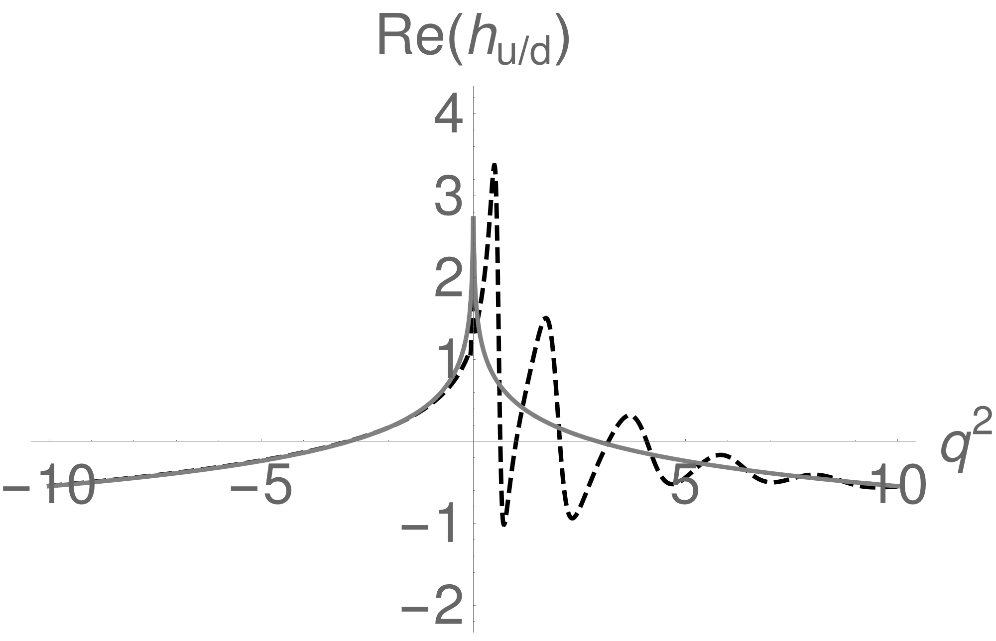
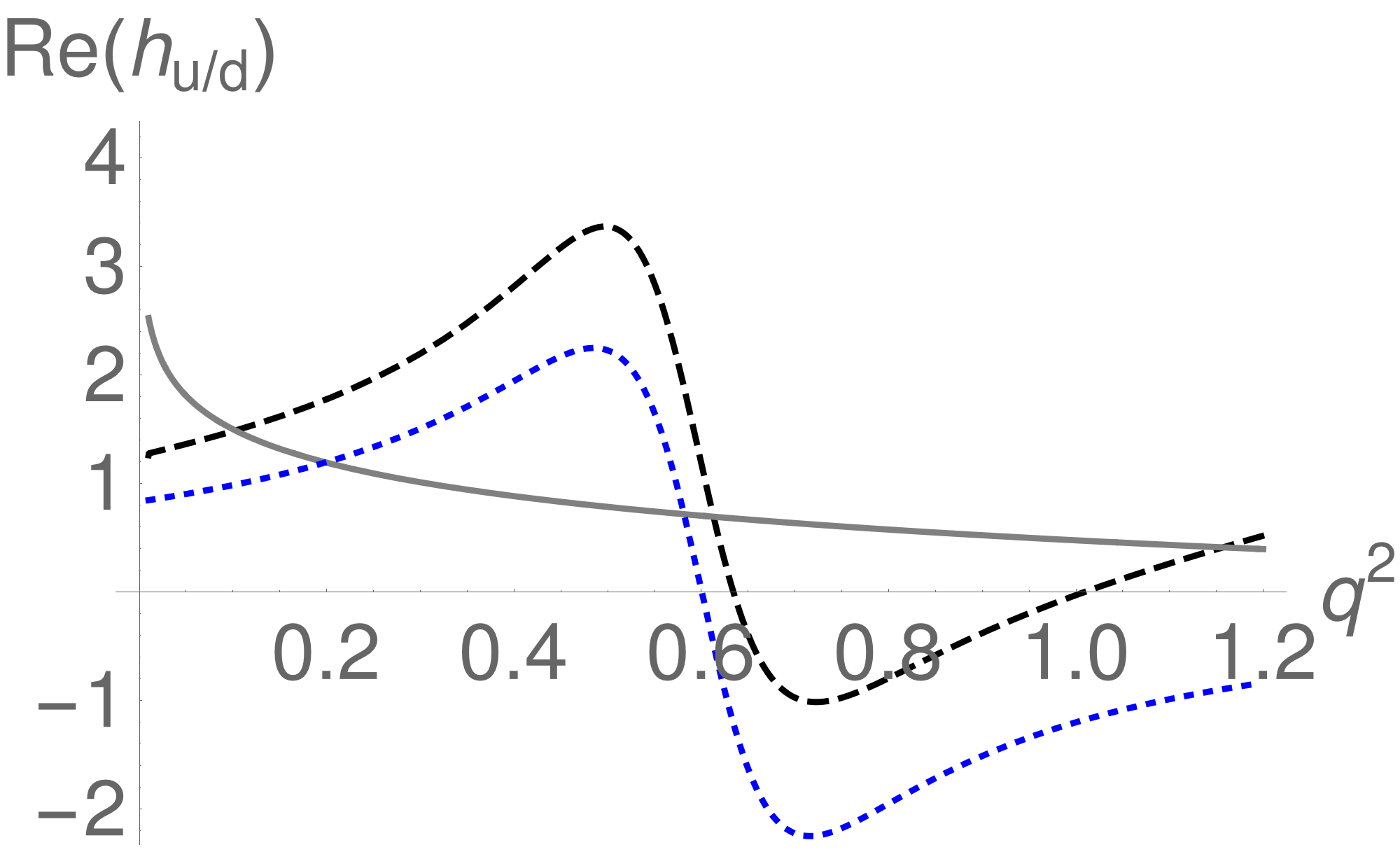
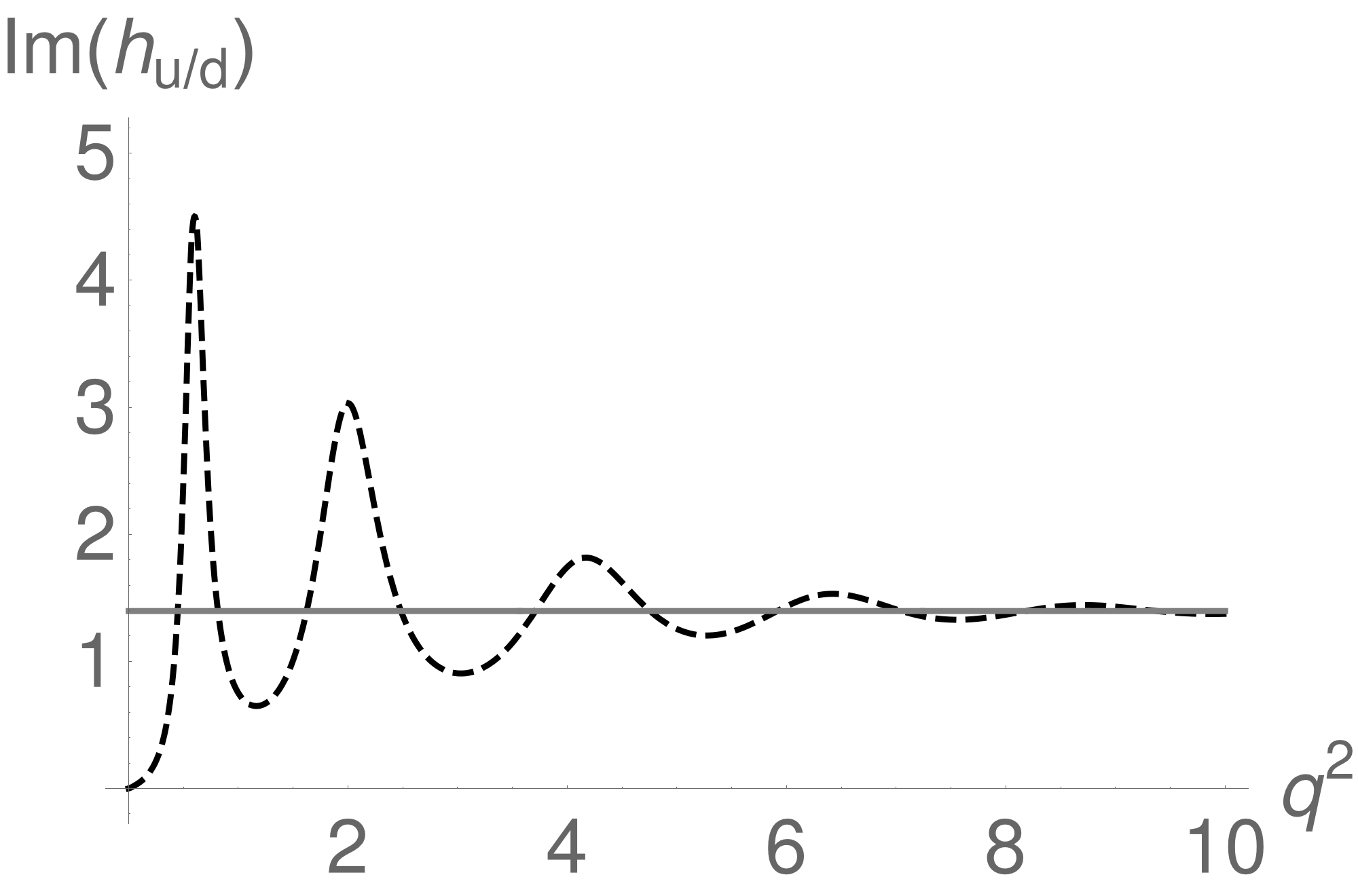
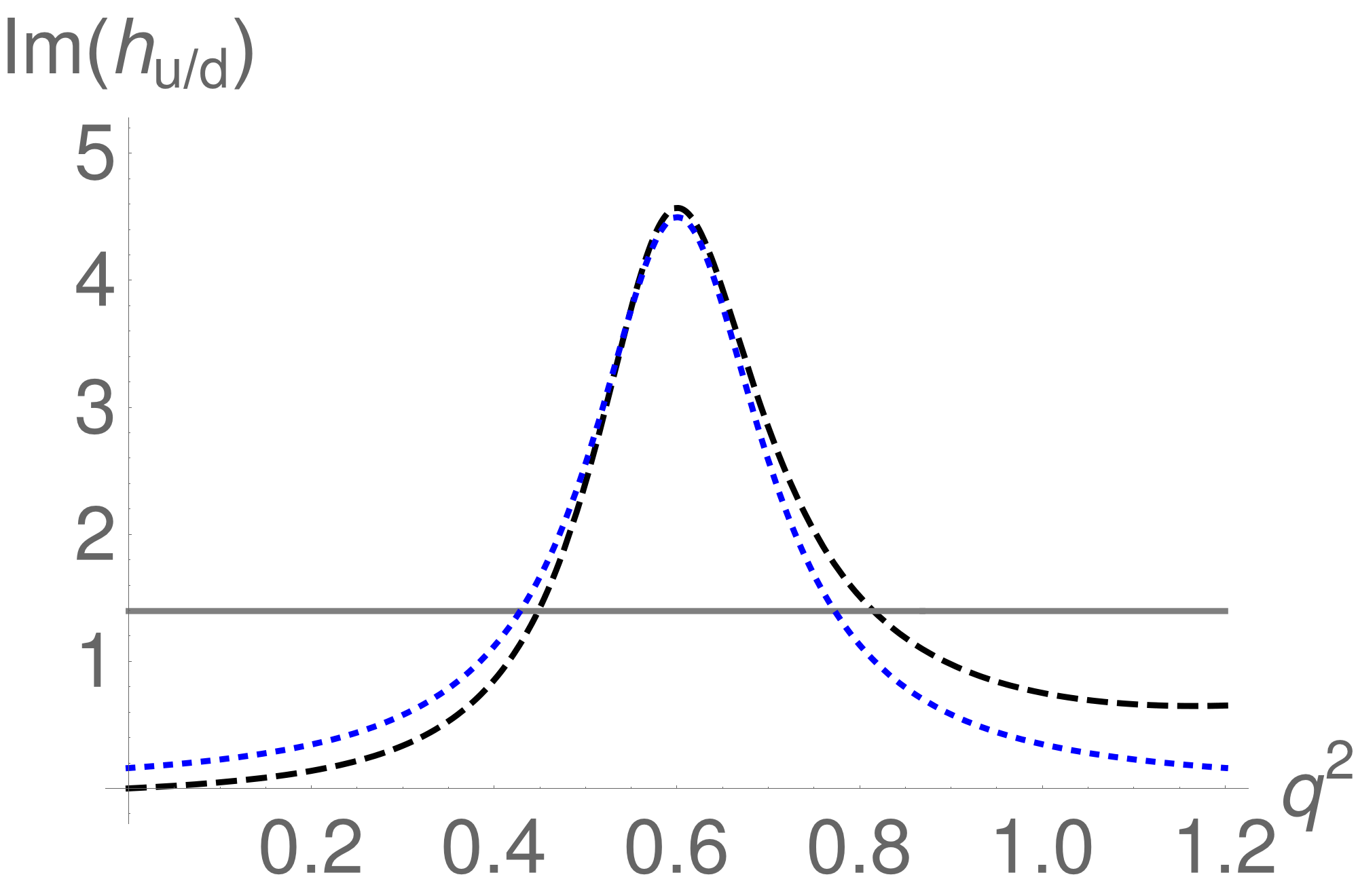
Figure 9: Comparison of the perturbative result for the real and imaginary part of the function $h(q^{2},0)$ (gray solid line) and the model (32) using (80) for its hadronic modification (black dashed line) as a function of $q^{2}$ (in units of GeV²). On the right-hand side, we also compare to the simple Breit-Wigner ansatz (blue dotted line). The parameter values are chosen as follows: $\sigma^{2}=2~{}\text{GeV}^{2}$, $a=1$, $b=1/6$, $\mu^{2}=1.5$ GeV². The value of $n_{V}=1.94$ is tuned to reproduce the perturbative result in the limit $q^{2}\to-\infty$.

 

  

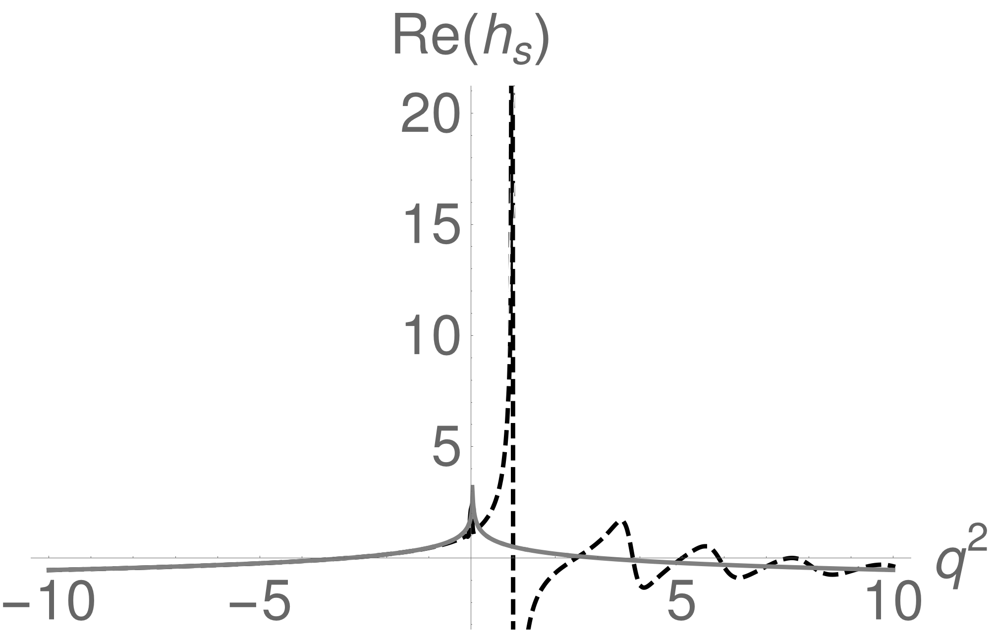
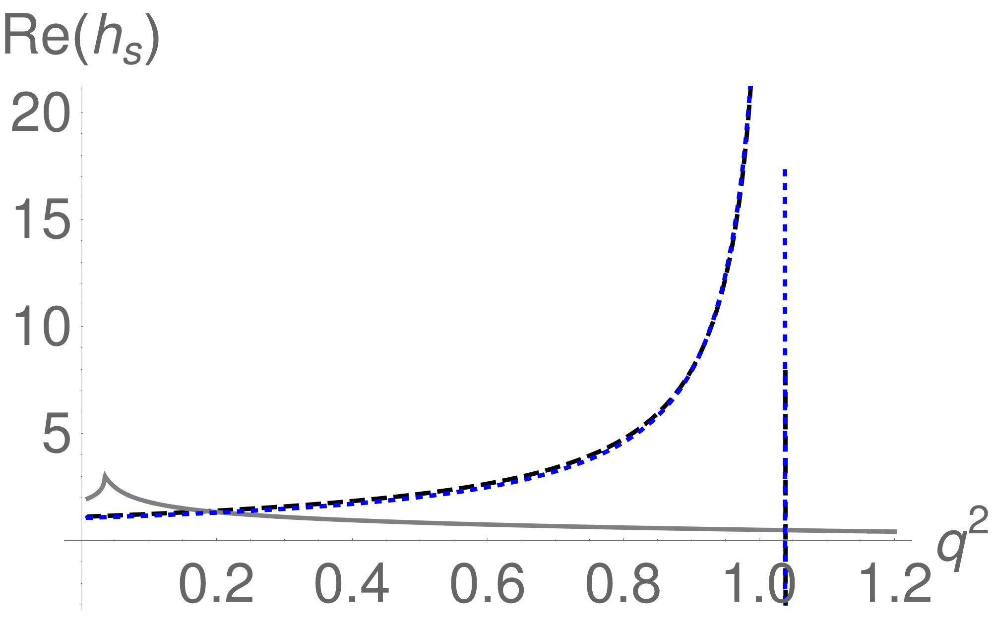
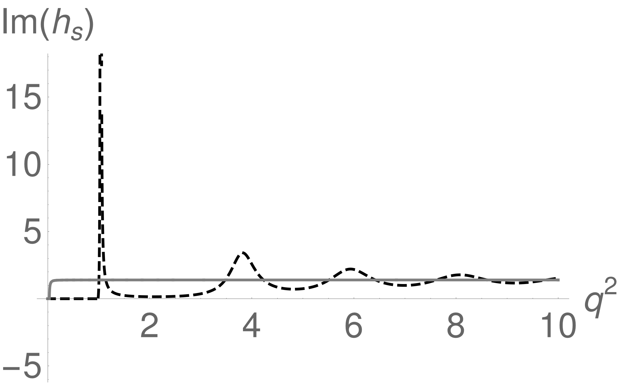
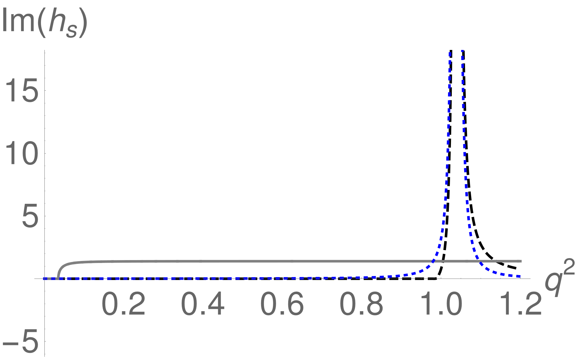
Figure 10: Comparison of the perturbative result for the real and imaginary part of the function $h(q^{2},m_{s})$ (gray solid line) and the model (32) using (80) for its hadronic modification (black dashed line) as a function of $q^{2}$ (in units of GeV²). On the right-hand side, we also compare to the simple Breit-Wigner ansatz (blue dotted line). The parameter values are chosen as follows: $\sigma^{2}=2~{}\text{GeV}^{2}$, $a_{s}=1.4$, $b_{s}=0.1$, $\mu^{2}=1.5$ GeV². The parameter $n_{\phi}=2.37$ is tuned to reproduce the perturbative result in the limit $q^{2}\to-\infty$.

B.2 Application to annihilation topology

In the QCDF approach, the leading contributions to the annihilation topology are determined by the functions

$$\left(\lambda_{D}^{\pm}(q^{2})\right)^{-1} =\int_{0}^{\infty}\frac{d\omega}{\omega-q^{2}/m_{D}-i\epsilon}\,\phi_{D}^{\pm}(\omega)\,.$$ (93)

To the level of accuracy that we are working with, it is sufficient to neglect 3-particle LCDAs in the $D$-meson. In that case the LCDAs $\phi_{D}^{\pm}(\omega)$ are not independent, but fulfill a so-called Wandzura-Wilczek relation Beneke:2000wa ,

$$\phi_{D}^{+}(\omega) \simeq-\omega\,\frac{d\phi_{D}^{-}(\omega)}{d\omega}\,,$$ (94)

which for the above moment implies

$$-q^{2}\,\frac{\partial}{\partial q^{2}}\left[\lambda_{D}^{-}(q^{2})\right]^{-1} =\left[\lambda_{D}^{+}(q^{2})\right]^{-1}\,.$$ (95)

Moreover, an alternative representation of the moments can be achieved in terms of the “Wandzura-Wilczek” wave function $\psi_{D}(x)$ as defined in Bell:2013tfa , where

$$\phi_{D}^{+}(\omega) =\omega\,\int_{\omega}^{\infty}dx\,\psi_{D}(x)\,,\qquad\phi_{D}^{-}(\omega)=\int_{\omega}^{\infty}dx\,(x-\omega)\,\psi_{D}(x)\,,$$ (96)

and $x$ is twice the energy of the spectator quark in the $D$-meson. With this, one has

$$\left(\lambda_{D}^{+}(q^{2})\right)^{-1} =\int_{0}^{\infty}dx\left[x+\frac{q^{2}}{m_{D}}\,\ln\left(1-\frac{m_{D}\,x}{q^{2}+i\epsilon}\right)\right]\psi_{D}(x)\,,$$ (97)

$$\left(\lambda_{D}^{-}(q^{2})\right)^{-1} =\int_{0}^{\infty}dx\,x\,\ln\left(1-\frac{m_{D}\,x}{q^{2}+i\epsilon}\right)\psi_{D}(x)-\left(\lambda_{D}^{+}(q^{2})\right)^{-1}\,.$$ (98)

Looking at the analytic properties of these expressions, one easily verifies that

$$\frac{1}{\pi}{\rm Im}\left(\lambda_{D}^{+}(q^{2})\right)^{-1} =\int_{0}^{\infty}dx\,\theta(q^{2})\,\theta(m_{D}x-q^{2})\,\frac{q^{2}}{m_{D}}\,\psi_{D}(x)=\theta(q^{2})\,\phi_{D}^{+}(q^{2}/m_{D})\,,$$ (99)

$$\frac{1}{\pi}{\rm Im}\left(\lambda_{D}^{-}(q^{2})\right)^{-1} =\int_{0}^{\infty}dx\,\theta(q^{2})\,\theta(m_{D}x-q^{2})\left(x-\frac{q^{2}}{m_{D}}\right)\psi_{D}(x)=\theta(q^{2})\,\phi_{D}^{-}(q^{2}/m_{D})\,,$$ (100)

and also (95) holds by simple differentiation. As a naive ansatz we may simply replace $\theta(q^{2})$ on the right-hand side of the above equations by the same function $j_{q}(q^{2})$ that has been used to model the hadronic spectrum for the function $h(q^{2},m_{q})$ in the previous subsection. This corresponds to the naive factorization into the subprocesses $D\to\rho q\bar{q}$ (described in QCDF in terms of $\phi_{D}^{\pm}$) followed by $q\bar{q}\to\gamma^{*}$ (described by the resonance model). With this, we take

$$\left(\lambda_{D}^{\pm}(q^{2})\right)^{-1} \to\int_{0}^{\infty}\frac{ds}{s-q^{2}-i\epsilon}\,\phi_{D}^{\pm}(s/m_{D})\,j_{u/d}(s)\,.$$

As before, we tune the parameter $n_{V}$ (independently for both cases) to reproduce the asymptotic limit $q^{2}\ll-m_{D}\Lambda$, i.e. we require

$$\int_{0}^{\infty}ds\,\phi_{D}^{\pm}(s/m_{D})\big{(}j_{u/d}(s)-1\big{)} \stackrel{{\scriptstyle!}}{{=}}0\,.$$ (102)

Using an exponential model (38) for the $D$-meson LCDAs with $\omega_{0}=0.45$ GeV, we obtain $n_{V}=2.40$ for $\lambda_{D}^{-}(q^{2})$ and $n_{V}=1.75$ for $\lambda_{D}^{+}(q^{2})$, respectively. The comparison between the perturbative result and the hadronic model is shown in Figs. 11,12, see also the discussion around Figs. 5,6 in the main text.

We may again analyze our model for $\lambda_{D}^{\pm}(q^{2})$ in the framework of QCD sum rules. With the analogous steps as in (90) this leads to

$$\frac{n_{V}\,M_{V}^{2}}{M_{V}^{2}-q^{2}}\,\phi_{D}^{\pm}(M_{V}^{2}/m_{D}) \simeq\int_{0}^{s_{0}}ds\,\frac{1}{s-q^{2}-i\epsilon}\,\phi_{D}^{\pm}(s/m_{D})\,\theta(s)\,,$$ (103)

and after Borel transformation one has

$$e^{-M_{V}^{2}/M^{2}}\,n_{V}\,M_{V}^{2}\,\phi_{D}^{\pm}(M_{V}^{2}/m_{D}) \simeq\int_{0}^{s_{0}}ds\,e^{-s/M^{2}}\,\phi_{D}^{\pm}(s/m_{D})\,.$$ (104)

In the heavy-mass limit, $m_{D}\cdot\langle\omega\rangle\gg s_{0}\sim M^{2}$, one can expand the LCDAs,

$$\phi_{D}^{-}(\omega)\simeq\phi_{D}^{-}(0)\,,\qquad\phi_{D}^{+}(\omega)\simeq\omega\,\phi_{D}^{+}{}^{\prime}(0)\,,$$

and (104) reduces to

$$M_{V}^{2}\,n_{V} =M^{2}\,e^{M_{V}^{2}/M^{2}}\left(1-e^{-s_{0}/M^{2}}\right)$$ (105)

$$=4\pi^{2}\,f_{V}^{2}\qquad\left[\mbox{for $\lambda_{D}^{-}(q^{2})$}\right],$$ (106)

respectively,

$$M_{V}^{2}\,n_{V} =\frac{M^{2}}{M_{V}^{2}}\,e^{M_{V}^{2}/M^{2}}\left(M^{2}-e^{-s_{0}/M^{2}}\,(s_{0}+M^{2})\right)$$ (107)

$$=4\pi^{2}f_{V}^{2}\,\frac{M^{2}}{M_{V}^{2}}\frac{1-e^{-s_{0}/M^{2}}\,(1+s_{0}/M^{2})}{1-e^{-s_{0}/M^{2}}}\qquad\left[\mbox{for $\lambda_{D}^{+}(q^{2})$}\right].$$ (108)

Again, within the intrinsic uncertainties, the numerical values for $n_{V}$ fitted to the asymptotic behaviour of $\lambda_{D}^{\pm}(q^{2})$ are consistent with the above findings (without going into details of the sum-rule analysis). In particular, by comparing Eqs. (106) and (92), the value of $n_{V}$ – to first approximation – is expected to be universal for the modelling of $h(s,m_{q})$ and $\lambda_{D}^{-}(q^{2})$.

 

 

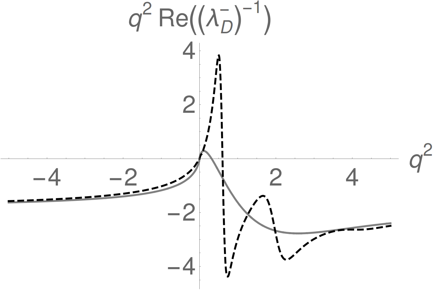
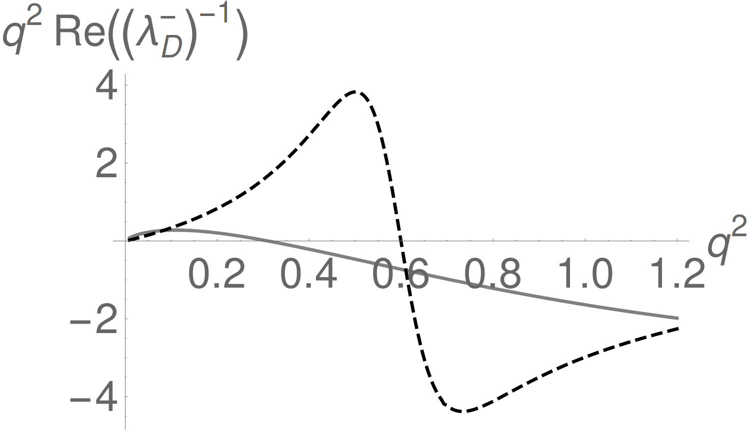
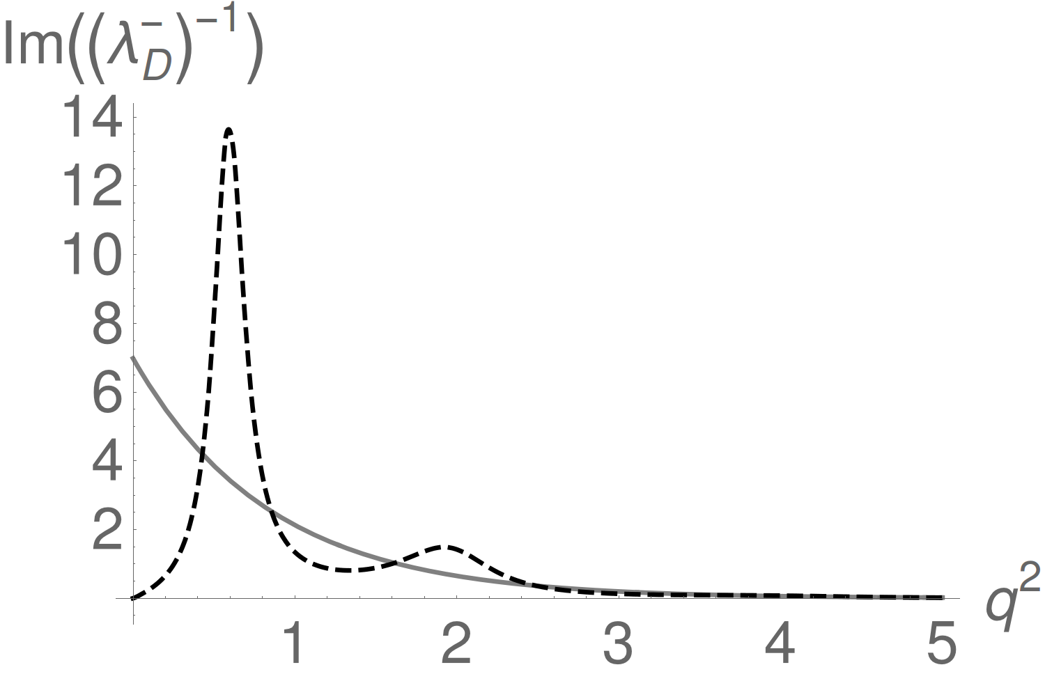
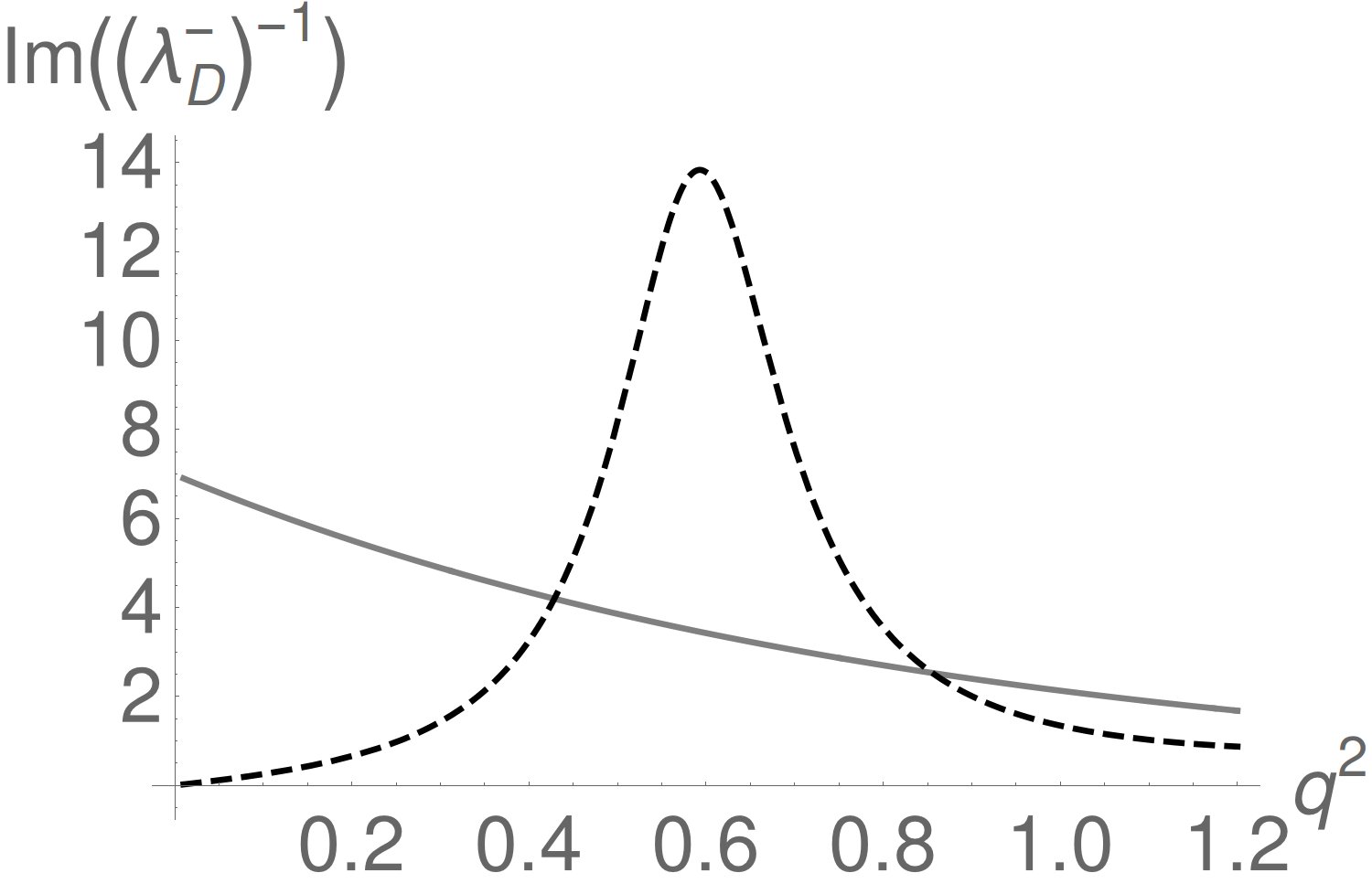
Figure 11: Comparison of the perturbative result for the real and imaginary part of the function $\left(\lambda_{D}^{-}(q^{2})\right)^{-1}$ (massless spectator, gray solid line) and the model (37) for its hadronic modification (black dashed line) as a function of $q^{2}$ (in units of GeV²). Notice that the real part has been multiplied by $q^{2}$. The parameter values are chosen as follows: $\sigma^{2}=2~{}\text{GeV}^{2}$, $a=1$, $b=1/6$. The $D$-meson LCDA is modelled by an exponential (38) with $\omega_{0}=0.45$ GeV. The parameter $n_{V}=2.40$ is tuned to reproduce the result for deep Euclidean values of $q^{2}$.

 

 

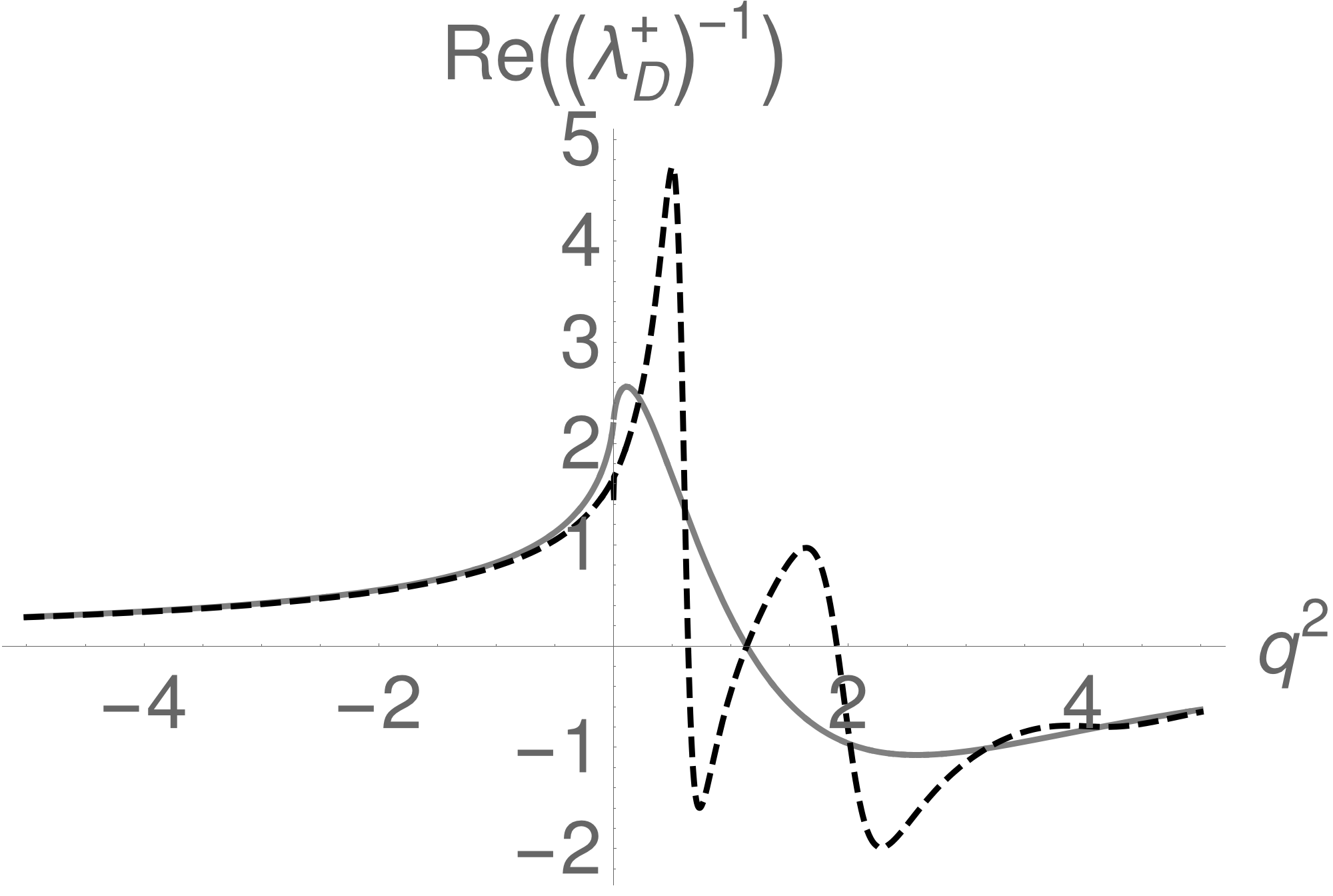
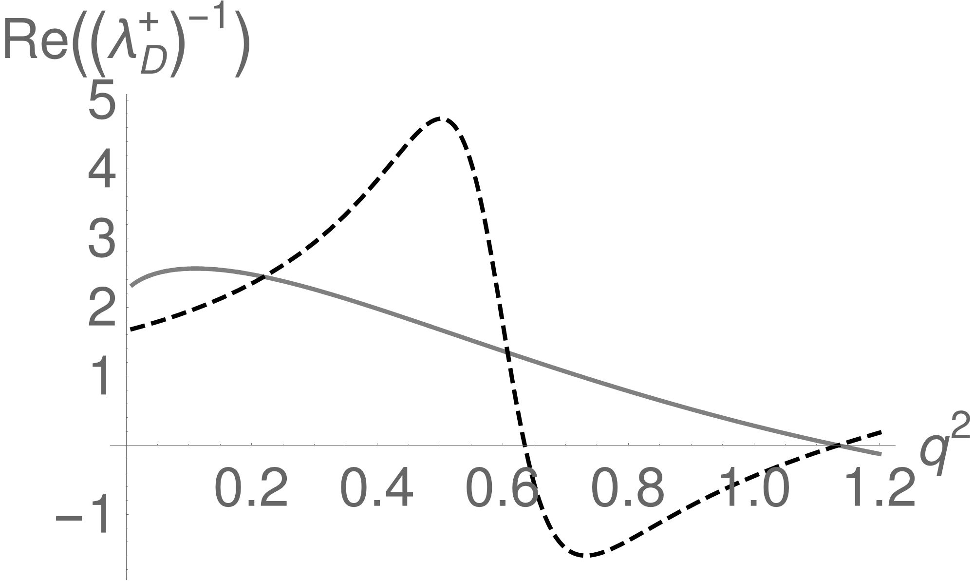
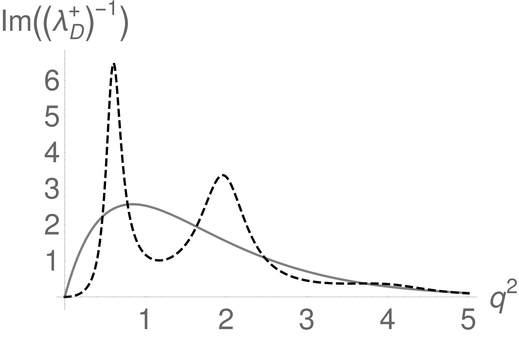
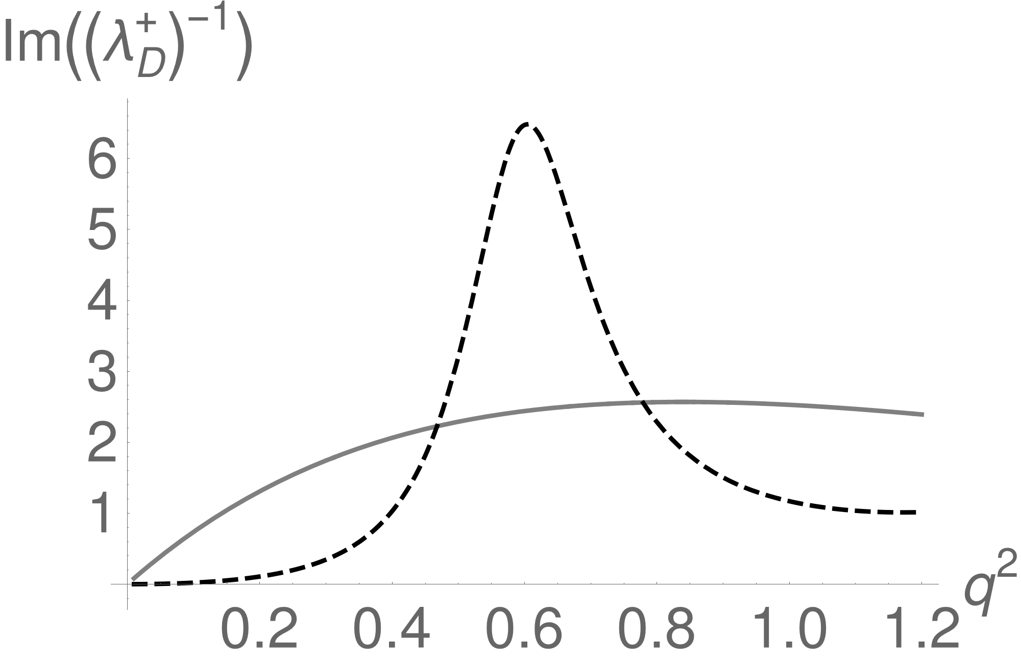
Figure 12: Comparison of the perturbative result for the real and imaginary part of the function $\left(\lambda_{D}^{+}(q^{2})\right)^{-1}$ (massless spectator, gray solid line) and the model (42) for its hadronic modification (black dashed line) as a function of $q^{2}$ (in units of GeV²). The parameter values are chosen as follows: $\sigma^{2}=2~{}\text{GeV}^{2}$, $a=1$, $b=1/6$. The $D$-meson LCDA is modelled by an exponential with $\omega_{0}=0.45$ GeV. The parameter $n_{V}=1.75$ is tuned to reproduce the result for deep Euclidean values of $q^{2}$.

Appendix C More Input Parameters

In Table 11 we summarize a number of input parameters that have been used in the numerical analyses. The parameters describing the $q^{2}$-dependence of the the $D\to\rho$ form factors are quoted after Eq. (22) in the main body of the text.

$\alpha_{\rm{em}}$	$1/137$
$\bar{m}_{c}(\bar{m}_{c})$	$1.275$ GeV
$\bar{m}_{s}(2\,\rm{GeV})$	$93.5$ MeV
$M_{D^{\pm}}$	$1.870$ GeV
$M_{D^{0}}$	$1.865$ GeV
$\tau_{D^{\pm}}$	$1.04$ ps
$\tau_{D^{0}}$	$0.41$ ps
$M_{D^{*\pm}}$	$2.010$ GeV
$M_{D^{*0}}$	$2.007$ GeV

$m_{\rho}$	$0.775$ GeV
$\Gamma_{\rho}$	$0.149$ GeV
$m_{\phi}$	$1.019$ GeV
$\Gamma_{\phi}$	$4.26$ MeV
$m_{K}$	$0.497$ GeV
$\lambda$	$0.22506$
$A$	$0.811$
$\bar{\rho}$	$0.124$
$\bar{\eta}$	$0.356$

Table 11: Summary of input parameters not quoted in Table 2. All values taken from PDG . (Here $\lambda$, $A$, $\bar{\rho}$, $\bar{\eta}$ are the Wolfenstein parameters for the CKM matrix.)

References

- (1) M. Antonelli et. al., Flavor Physics in the Quark Sector, Phys. Rept. 494 (2010) 197–414 [0907.5386].
- (2) LHCb Collaboration, R. Aaij et. al., Implications of LHCb measurements and future prospects, Eur. Phys. J. C73 (2013), no. 4 2373 [1208.3355].
- (3) M. Artuso et. al., , and decays, Eur. Phys. J. C57 (2008) 309–492 [0801.1833].
- (4) S. Fajfer, S. Prelovsek and P. Singer, Rare charm meson decays and in SM and MSSM, Phys. Rev. D64 (2001) 114009 [hep-ph/0106333].
- (5) G. Burdman, E. Golowich, J. L. Hewett and S. Pakvasa, Rare charm decays in the standard model and beyond, Phys. Rev. D66 (2002) 014009 [hep-ph/0112235].
- (6) S. Fajfer and S. Prelovsek, Effects of littlest Higgs model in rare D meson decays, Phys. Rev. D73 (2006) 054026 [hep-ph/0511048].
- (7) S. Fajfer, N. Kosnik and S. Prelovsek, Updated constraints on new physics in rare charm decays, Phys. Rev. D76 (2007) 074010 [0706.1133].
- (8) A. Paul, I. I. Bigi and S. Recksiegel, On within the Standard Model and Frameworks like the Littlest Higgs Model with T Parity, Phys. Rev. D83 (2011) 114006 [1101.6053].
- (9) L. Cappiello, O. Cata and G. D’Ambrosio, Standard Model prediction and new physics tests for , JHEP 04 (2013) 135 [1209.4235].
- (10) G. Isidori and J. F. Kamenik, Shedding light on CP violation in the charm system via decays, Phys. Rev. Lett. 109 (2012) 171801 [1205.3164].
- (11) J. Lyon and R. Zwicky, Anomalously large and long-distance chirality from , 1210.6546.
- (12) S. Fajfer and N. Kosnik, Resonance catalyzed CP asymmetries in , Phys. Rev. D87 (2013), no. 5 054026 [1208.0759].
- (13) S. Fajfer and N. Kosnik, Prospects of discovering new physics in rare charm decays, Eur. Phys. J. C75 (2015), no. 12 567 [1510.00965].
- (14) S. de Boer and G. Hiller, Flavor and new physics opportunities with rare charm decays into leptons, Phys. Rev. D93 (2016), no. 7 074001 [1510.00311].
- (15) S. de Boer and G. Hiller, Rare radiative charm decays within the standard model and beyond, 1701.06392.
- (16) A. Biswas, S. Mandal and N. Sinha, Searching for New physics in Charm Radiative decays, 1702.05059.
- (17) C. Greub, T. Hurth, M. Misiak and D. Wyler, The contribution to weak radiative charm decay, Phys. Lett. B382 (1996) 415–420 [hep-ph/9603417].
- (18) S. de Boer, B. Müller and D. Seidel, Higher-order Wilson coefficients for transitions in the Standard Model, 1606.05521.
- (19) M. Beneke, T. Feldmann and D. Seidel, Systematic approach to exclusive , decays, Nucl. Phys. B612 (2001) 25–58 [hep-ph/0106067].
- (20) S. W. Bosch and G. Buchalla, The Radiative decays at next-to-leading order in QCD, Nucl. Phys. B621 (2002) 459–478 [hep-ph/0106081].
- (21) A. Ali and A. Y. Parkhomenko, Branching ratios for and decays in next-to-leading order in the large energy effective theory, Eur. Phys. J. C23 (2002) 89–112 [hep-ph/0105302].
- (22) A. L. Kagan and M. Neubert, Isospin breaking in decays, Phys. Lett. B539 (2002) 227–234 [hep-ph/0110078].
- (23) T. Feldmann and J. Matias, Forward backward and isospin asymmetry for decay in the standard model and in supersymmetry, JHEP 01 (2003) 074 [hep-ph/0212158].
- (24) M. Beneke, T. Feldmann and D. Seidel, Exclusive radiative and electroweak and penguin decays at NLO, Eur. Phys. J. C41 (2005) 173–188 [hep-ph/0412400].
- (25) A. Ali, B. D. Pecjak and C. Greub, V Decays at NNLO in SCET, Eur. Phys. J. C55 (2008) 577–595 [0709.4422].
- (26) M. Bartsch, M. Beylich, G. Buchalla and D. N. Gao, Precision Flavour Physics with and , JHEP 11 (2009) 011 [0909.1512].
- (27) S. Jäger and J. Martin Camalich, On at small dilepton invariant mass, power corrections, and new physics, JHEP 05 (2013) 043 [1212.2263].
- (28) G. Buchalla and G. Isidori, Nonperturbative effects in for large dilepton invariant mass, Nucl. Phys. B525 (1998) 333–349 [hep-ph/9801456].
- (29) B. Grinstein and D. Pirjol, Exclusive rare decays at low recoil: Controlling the long-distance effects, Phys. Rev. D70 (2004) 114005 [hep-ph/0404250].
- (30) M. Beylich, G. Buchalla and T. Feldmann, Theory of decays at high : OPE and quark-hadron duality, Eur. Phys. J. C71 (2011) 1635 [1101.5118].
- (31) A. Khodjamirian, T. Mannel, A. A. Pivovarov and Y. M. Wang, Charm-loop effect in and , JHEP 09 (2010) 089 [1006.4945].
- (32) J. Lyon and R. Zwicky, Resonances gone topsy turvy - the charm of QCD or new physics in ?, 1406.0566.
- (33) LHCb Collaboration, R. Aaij et. al., Observation of a resonance in decays at low recoil, Phys. Rev. Lett. 111 (2013), no. 11 112003 [1307.7595].
- (34) M. Beneke, G. Buchalla, M. Neubert and C. T. Sachrajda, QCD factorization for decays: Strong phases and CP violation in the heavy quark limit, Phys. Rev. Lett. 83 (1999) 1914–1917 [hep-ph/9905312].
- (35) M. Beneke, G. Buchalla, M. Neubert and C. T. Sachrajda, QCD factorization in decays and extraction of Wolfenstein parameters, Nucl. Phys. B606 (2001) 245–321 [hep-ph/0104110].
- (36) B. Blok, M. A. Shifman and D.-X. Zhang, An Illustrative example of how quark hadron duality might work, Phys. Rev. D57 (1998) 2691–2700 [hep-ph/9709333]. [Erratum: Phys. Rev.D59,019901(1999)].
- (37) M. A. Shifman, Quark hadron duality, in Proceedings, 8th International Symposium on Heavy Flavor Physics (Heavy Flavors 8), p. hf8/013, 2000. hep-ph/0009131.
- (38) M. Shifman, The quark hadron duality, eConf C030614 (2003) 001.
- (39) K. G. Chetyrkin, M. Misiak and M. Münz, nonleptonic effective Hamiltonian in a simpler scheme, Nucl. Phys. B520 (1998) 279–297 [hep-ph/9711280].
- (40) D. Seidel, Analytic two loop virtual corrections to , Phys. Rev. D70 (2004) 094038 [hep-ph/0403185].
- (41) M. Beneke and T. Feldmann, Symmetry breaking corrections to heavy to light B meson form-factors at large recoil, Nucl. Phys. B592 (2001) 3–34 [hep-ph/0008255].
- (42) G. Buchalla, Precision flavour physics with and , Nucl. Phys. Proc. Suppl. 209 (2010) 137–142 [1010.2674].
- (43) CLEO Collaboration, S. Dobbs et. al., First Measurement of the Form Factors in the Decays and , Phys. Rev. Lett. 110 (2013), no. 13 131802 [1112.2884].
- (44) S. Fajfer and J. F. Kamenik, Charm meson resonances and semileptonic form-factors, Phys. Rev. D72 (2005) 034029 [hep-ph/0506051].
- (45) G. Buchalla, A. J. Buras and M. E. Lautenbacher, Weak decays beyond leading logarithms, Rev. Mod. Phys. 68 (1996) 1125–1144 [hep-ph/9512380].
- (46) A. Khodjamirian, G. Stoll and D. Wyler, Calculation of long distance effects in exclusive weak radiative decays of B meson, Phys. Lett. B358 (1995) 129–138 [hep-ph/9506242].
- (47) P. Gambino, M. Gorbahn and U. Haisch, Anomalous dimension matrix for radiative and rare semileptonic B decays up to three loops, Nucl. Phys. B673 (2003) 238–262 [hep-ph/0306079].
- (48) C. Greub, V. Pilipp and C. Schupbach, Analytic calculation of two-loop QCD corrections to in the high region, JHEP 12 (2008) 040 [0810.4077].
- (49) C. Greub, T. Hurth and D. Wyler, Virtual corrections to the inclusive decay , Phys. Rev. D54 (1996) 3350–3364 [hep-ph/9603404].
- (50) A. G. Grozin and M. Neubert, Asymptotics of heavy meson form-factors, Phys. Rev. D55 (1997) 272–290 [hep-ph/9607366].
- (51) V. M. Braun and A. Khodjamirian, Soft contribution to and the -meson distribution amplitude, Phys. Lett. B718 (2013) 1014–1019 [1210.4453].
- (52) M. Beneke and J. Rohrwild, -meson distribution amplitude from , Eur. Phys. J. C71 (2011) 1818 [1110.3228].
- (53) Particle Data Group Collaboration, C. Patrignani et. al., Review of Particle Physics, Chin. Phys. C40 (2016), no. 10 100001.
- (54) P. Ball and R. Zwicky, from , JHEP 04 (2006) 046 [hep-ph/0603232].
- (55) A. Vladikas, FLAG: Lattice QCD Tests of the Standard Model and Foretaste for Beyond, PoS FPCP2015 (2015) 016 [1509.01155].
- (56) F. Krüger and J. Matias, Probing new physics via the transverse amplitudes of at large recoil, Phys. Rev. D71 (2005) 094009 [hep-ph/0502060].
- (57) Belle Collaboration, A. Abdesselam et. al., Observation of and search for violation in radiative charm decays, Phys. Rev. Lett. 118 (2017), no. 5 051801 [1603.03257].
- (58) O. Cata, M. Golterman and S. Peris, Duality violations and spectral sum rules, JHEP 08 (2005) 076 [hep-ph/0506004].
- (59) O. Cata, M. Golterman and S. Peris, Unraveling duality violations in hadronic decays, Phys. Rev. D77 (2008) 093006 [0803.0246].
- (60) O. Cata, M. Golterman and S. Peris, Possible duality violations in decay and their impact on the determination of , Phys. Rev. D79 (2009) 053002 [0812.2285].
- (61) D. Boito, O. Cata, M. Golterman, M. Jamin, K. Maltman, J. Osborne and S. Peris, A new determination of from hadronic decays, Phys. Rev. D84 (2011) 113006 [1110.1127].
- (62) P. Colangelo and A. Khodjamirian, QCD sum rules, a modern perspective, hep-ph/0010175.
- (63) G. Bell, T. Feldmann, Y.-M. Wang and M. W. Y. Yip, Light-Cone Distribution Amplitudes for Heavy-Quark Hadrons, JHEP 11 (2013) 191 [1308.6114].
- (64) M. Dimou, J. Lyon and R. Zwicky, Exclusive Chromomagnetism in heavy-to-light FCNCs, Phys. Rev. D87 (2013), no. 7 074008 [1212.2242].
- (65) F. De Fazio, T. Feldmann and T. Hurth, Light-cone sum rules in soft-collinear effective theory, Nucl. Phys. B733 (2006) 1–30 [hep-ph/0504088]. [Erratum: Nucl. Phys.B800,405(2008)].
- (66) F. De Fazio, T. Feldmann and T. Hurth, SCET sum rules for and transition form factors, JHEP 02 (2008) 031 [0711.3999].