The population of white dwarf-main sequence binaries in the SDSS DR 12

Abstract

We present a Monte Carlo population synthesis study of white dwarf-main sequence (WD+MS) binaries in the Galactic disk aimed at reproducing the ensemble properties of the entire population observed by the Sloan Digital Sky Survey (SDSS) Data Release 12. Our simulations take into account all known observational biases and use the most up-to-date stellar evolutionary models. This allows us to perform a sound comparison between the simulations and the observational data. We find that the properties of the simulated and observed parameter distributions agree best when assuming low values of the common envelope efficiency (0.2–0.3), a result that is in agreement with previous findings obtained by observational and population synthesis studies of close SDSS WD+MS binaries. We also show that all synthetic populations that result from adopting an initial mass ratio distribution with a positive slope are excluded by observations. Finally, we confirm that the properties of the simulated WD+MS binary populations are nearly independent of the age adopted for the thin disk, on the contribution of WD+MS binaries from the thick disk (0–17 per cent of the total population) and on the assumed fraction of the internal energy that is used to eject the envelope during the common envelope phase (0.1–0.5).

1 Introduction

White dwarf-main sequence (WD+MS) binaries are the evolutionary products of main sequence binaries. In $\sim$75 per cent of the cases the initial main sequence binary separations are large enough for the binary components to evolve in the same way as if they were single stars (Willems & Kolb, 2004). The orbital separations of the remaining $\sim$25 per cent of main sequence binaries are close enough for the systems to undergo a phase of dynamically unstable mass transfer once the primary becomes a red giant or an asymptotic giant branch star. This leads to the formation of a common envelope around the nucleus of the giant star and the main sequence companion (Webbink, 2008), and hence to a dramatic decrease of the orbital separation. WD+MS binaries that evolved through a common envelope phase are known as post-common envelope binaries (PCEBs).

Modern large scale surveys such as the Sloan Digital Sky Survey (York et al., 2000), the UKIRT Infrared Sky Survey (Dye et al., 2006) and the Large sky Area Multi-Object fiber Spectroscopic Telescope (LAMOST) survey (Zhao et al., 2012), have facilitated the compilation of comprehensive spectroscopic WD+MS binary samples during the last few years (Heller et al., 2009; Rebassa-Mansergas et al., 2010; Rebassa-Mansergas et al., 2012a; Liu et al., 2012; Rebassa-Mansergas et al., 2013; Ren et al., 2014). The SDSS has been a particularly rich source for the discovery of WD+MS binaries, mainly due to their overlap in colour space with quasars (Smolčić et al., 2004). Roughly 25 per cent of the SDSS WD+MS binaries are PCEBs (Nebot Gómez-Morán et al., 2011), some of which have been identified to be eclipsing (Nebot Gómez-Morán et al., 2009; Pyrzas et al., 2009; Parsons et al., 2013, 2015). The largest and most homogeneous catalogue of WD+MS binaries currently available is that from Rebassa-Mansergas et al. (2016a), with a total number 3291 systems identified within the data release 12 of SDSS.

Observationally, SDSS WD+MS binaries have been used as tools for analyzing several open and interesting problems. These include, for example, constraining theories of close compact binary evolution (Zorotovic et al., 2010; Davis et al., 2010; De Marco et al., 2011; Zorotovic et al., 2011; Rebassa-Mansergas et al., 2012b), providing observational confirmation for disrupted magnetic braking (Schreiber et al., 2010; Zorotovic et al., 2016), rendering robust evidence for the majority of low-mass white dwarfs being formed in binaries (Rebassa-Mansergas et al., 2011), studying the pairing properties of main sequence stars (Ferrario, 2012), using WD+MS binaries as new gravitational wave verification sources (Kilic et al., 2014), testing the existence of an age-metallicity relation in the Galactic disk (Rebassa-Mansergas et al., 2016b), using SDSS eclipsing PCEBs to test the existence of circumbinary planets (Zorotovic & Schreiber, 2013; Marsh et al., 2014).

Theoretically, population synthesis studies reproducing the ensemble properties of SDSS WD+MS binaries have been also highly successful at improving our current understanding of common envelope evolution (Toonen & Nelemans, 2013; Camacho et al., 2014; Zorotovic et al., 2014b). However, it is important to keep in mind that these works focused mainly on the PCEB sample observed by the SDSS. Clearly, far more can be learned from analyzing the total (PCEB plus wide WD+MS binary) population. In order to overcome this drawback, in this paper we present a suite of new simulations of the entire population of WD+MS binaries in the SDSS data release 12. To this end we employ an improved version of the population synthesis code used in Camacho et al. (2014). Our code is based in Monte Carlo techniques and takes into account all known observational biases and selection procedures. Also, we adopt different star formation histories, initial mass ratio distributions, common envelope efficiencies, thin disk ages and a variable contribution of WD+MS binaries from the thick disk. All this aims at constraining which set of parameters fit better the observational data.

The paper is organized as follows. In Section 2 we describe the observational sample of SDSS WD+MS binaries. In Section 3 we describe our Monte Carlo simulator and in Section 4 we explain how all known observational biases are implemented in our numerical simulations. In Section 5 we present our results. We close our paper by summarizing our main results and drawing our conclusions in Section 6.

2 The observed WD+MS sample

As already mentioned, the SDSS WD+MS binary catalogue currently constitutes the largest and most homogeneous sample of spectroscopic WD+MS binaries, with 3,291 systems identified within the data release 12 (Rebassa-Mansergas et al., 2016a). Because of selection effects, the vast majority of SDSS WD+MS binaries contain a low-mass M-dwarf secondary star, as hotter main sequence stars generally outshine the white dwarf in the optical SDSS spectrum (more details on this issue are provided in Section 4.3).

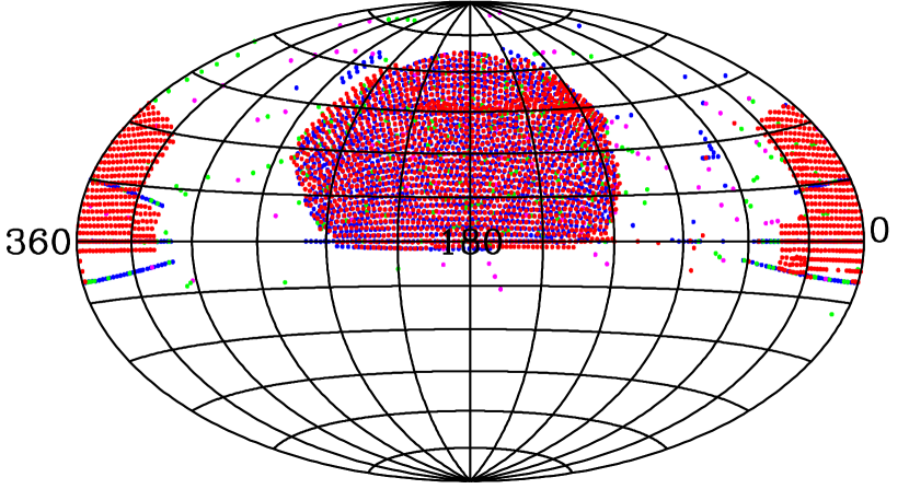
Figure 1: A Hammer-Aitoff projection in equatorial coordinates of the SDSS spectroscopic plate positions. Red dots indicate Legacy plates, blue dots are used for BOSS, green dots for SEGUE and magenta dots for SEGUE-2

The majority of SDSS WD+MS binaries have been observed as part of the Legacy Survey (Adelman-McCarthy et al., 2008; Abazajian et al., 2009) and BOSS (Barion Oscillation Spectroscopic Survey; Dawson et al., 2013) simply because of their overlap in colour space with quasars. Hence, Legacy and BOSS WD+MS binaries generally contain hot ($\gtrsim 10,000\,$K) white dwarfs. In order to overcome this observational bias, WD+MS binaries were additionally observed as part of a SEGUE — Sloan Exploration of Galactic Understanding and Evolution (Yanny et al., 2009) — dedicated survey aimed at targeting WD+MS binaries containing cool white dwarfs (Rebassa-Mansergas et al., 2012a). Hereafter, we flag these systems as SEGUE WD+MS binaries. Finally, a small number of WD+MS binaries were observed by the SEGUE and SEGUE-2 surveys of SDSS that aimed at obtaining spectra of main sequence stars and red giants. We flag these as SEGUE-2 WD+MS binaries.

White dwarf effective temperatures, surface gravities and masses and secondary star (M dwarf) spectral types were derived for each of the SDSS WD+MS binaries from their SDSS spectra using the decomposition/fitting routine described in Rebassa-Mansergas et al. (2007). Rebassa-Mansergas et al. (2016a) demonstrated that the stellar parameter distributions resulting from the four different sub-populations of SDSS WD+MS binaries (namely Legacy, BOSS, SEGUE and SEGUE-2 WD+MS binaries) are statistically different. This is a simple consequence of the different selection criteria and magnitude cuts employed by the four different sub-surveys. Thus, the overall SDSS WD+MS binary population is severely affected by selection effects. As a consequence, modeling the entire SDSS WD+MS binary sample entails some complications, as implementing the specific selection biases for each sub-sample is needed. Moreover, our simulations need to take into account that SDSS observed in specific regions of the sky, being these marked by the positions of the over 4,000 fibre-fed spectroscopic plates used during the observations (see Fig. 1).

3 The synthetic WD+MS sample

In this section we describe our Monte Carlo simulator and we provide details on our adopted evolutionary sequences and white dwarf cooling tracks.

3.1 The population synthesis code

To simulate the population of WD+MS binaries we employed an updated version of the population synthesis code designed to simulate both single and binary white dwarfs in the Galactic disk, first presented in Camacho et al. (2014) and built as an extension of a previous Monte Carlo code (García-Berro et al., 1999, 2004; Torres et al., 2005) specifically designed to study the population of single white dwarfs in the Galactic disk. In what follows we describe its main ingredients.

We start providing the initial conditions for any of the stars that constitute our population. These are the zero-age main sequence (ZAMS) mass sampled from the initial mass function (IMF) of Kroupa (2001), the time of birth obtained from the star formation history (SFH) — which is assumed to be constant in our reference model — the metallicity (assumed to be Solar), and a single or binary star membership according to an adopted binary fraction of 50 per cent (Duchêne & Kraus, 2013). If the star is member of a binary system we obtain the ZAMS mass of the secondary star according to an initial mass ratio distribution (IMRD) — which is assumed to be flat in our reference model. The initial separation of the binary is chosen from a logarithmically flat distribution (Davis et al., 2010) and the initial eccentricity from a linear thermal distribution (Heggie, 1975). We then assign a location (and, consequently, a distance) of the object. The equatorial coordinates for each of our synthetic star follow the distributions of all SDSS plates used up to the data release 12 (Fig. 1) adopting a solid angle aperture of 7 square degrees per plate. The radial distance from the Sun extends up to distances of 2 kpc. To distribute synthetic stars we employ a double exponential function for the local density of stars, with a scale height of 300 pc and a scale length of 2.6 kpc for the thin disk, and a 900 pc scale height and 3.5 kpc scale length for the thick disk (Bland-Hawthorn & Gerhard, 2016). Our density distribution is then normalized to the local mass density within 200 pc from the Sun, adopting standard values, namely $\rho_{\rm thin}=0.094\,M_{\sun}/{\rm pc^{3}}$ for the thin disk (Holmberg & Flynn, 2000) and thick disk — $\rho_{\rm thick}=8.5$ per cent of $\rho_{\rm thin}$ (Reid, 2005). We finally compute velocities in the standard right-handed Cartesian Galactic system where the mean space velocity components for the thin disk population are $(\langle U\rangle,\,\langle V\rangle\,,\langle W\rangle\,)=(-8.62\,,-20.04\,,-7.10)\,$km/s and its corresponding dispersions are $(\sigma_{U}\,,\sigma_{V},\sigma_{W})=(32.4\,,23.0\,,18.1)\,$km/s, while for the thick disk we adopt $(\langle U\rangle,\,\langle V\rangle\,,\langle W\rangle\,)=(-11.0\,,-42.0\,,-12.0\,)\,$km/s and $(\sigma_{U},\sigma_{V},\sigma_{W})=(50.0\,,54.0\,,34.0\,)\,$km/s — see Rowell & Hambly (2011) for details.

We then allow the synthetic single or binary system to evolve until present time, adopting for our reference model a thin disk age of 10 Gyr (Cojocaru et al., 2014) and a thick disk age of 12 Gyr. This is motivated by the findings of Feltzing & Bensby (2009) who presented a sample of very likely thick disk candidates with ages on average well above 10 Gyr and of Ak et al. (2013) who found that thick disk cataclysmic variables have ages up to 13 Gyr. If the synthetic star is single and has time to become a white dwarf, it evolves following the cooling tracks detailed in the following section. If that is the case, the mass of the white dwarf is obtained from the initial-to-final mass relation (IFMR) according to the prescription from Hurley et al. (2002). If the object is member of a binary system and the primary star has time to become a white dwarf, then the pair can evolve through two different scenarios. In the first scenario the binary evolves without mass transfer interactions as a detached system and the primary star evolves into a white dwarf that subsequently cools down following the cooling sequences described in the next section. In this case the mass of the white dwarf is also calculated from the initial-to-final mass relation of Hurley et al. (2002). The second scenario involves mass transfer episodes and the evolution of the binary is obtained following the prescriptions of the BSE package (Hurley et al., 2002), following the parameter assumptions detailed in Camacho et al. (2014). If the system evolves though the common envelope phase we use the $\alpha$-formalism as described in Tout et al. (1997), with $\alpha_{\mathrm{CE}}$ being the efficiency in converting orbital energy into kinetic energy to eject the envelope (assumed to be 0.3 in our reference model). This implementation also takes into account the $\alpha_{\mathrm{int}}$ parameter (assumed to be 0.0 in our reference model), first presented in Han et al. (1995), describing the fraction of the internal energy (thermal, radiation and recombination energy) used to eject the envelope. As described in Camacho et al. (2014), the $\alpha_{\mathrm{int}}$ parameter is used to include the effects of the internal energy in the binding energy parameter $\lambda$, which is thus not taken as a constant, but computed using a specific algorithm (Claeys et al., 2014) in BSE. In the current version of the code, provided that a positive value is used, the parameter $\alpha_{\mathrm{int}}$ represents the fraction of recombination energy that contributes to eject the envelope. It is important to note that the thermal energy of the envelope is always taken into account (using the virial theorem) even if $\alpha_{\mathrm{int}}$ is set to zero. For a more detailed discussion on how this is implemented in the latest version of BSE and important comments on the correct use of BSE and the notations used in the code itself, we direct the reader to Zorotovic et al. (2014a), mentioning that the notations $\alpha_{\mathrm{int}}$ or $\alpha_{\mathrm{rec}}$ are, in our case, equivalent.

3.2 Evolutionary sequences and cooling tracks

The BSE package (Hurley et al., 2002) provides luminosities, temperatures and surface gravities for both the main sequence and the white dwarf, computed using the evolutionary tracks of Pols et al. (1998) and a modified Mestel cooling law, respectively. We re-compute these stellar parameters using more modern tracks that also provide photometric magnitudes in the Johnson-Cousins $UBVRI$ system (taking into account both rejuvenation and ageing during overflow episodes). These evolutionary tracks are also used to derive the stellar parameters of the binary components in binaries where no mass transfer interactions take place.

For carbon-oxygen white dwarfs (that is, white dwarf with masses $M_{\rm{WD}}$ between $0.45$ and $1.10\,M_{\sun}$) we use the evolutionary calculations of Renedo et al. (2010), for oxygen-neon core white dwarfs (namely, white dwarfs with masses $M_{\rm{WD}}>1.1\,M_{\sun}$) we employ those of Althaus et al. (2005) and Althaus et al. (2007), and for helium core white dwarfs (with masses $M_{\rm{WD}}<0.45\,M_{\sun}$) we used the cooling tracks of Serenelli et al. (2001). In all cases Solar metallicity and hydrogen-rich atmospheres are assumed and the full set of $UBVRI$ magnitudes are provided.

For the main sequence companion we employ the new evolutionary tracks for low mass stars of Baraffe et al. (2015), which provide improved predictions for optical colours. The only downside here is that these sequences only provide the $VRI$ magnitudes, $U$ and $B$ magnitudes are recovered using a third order polynomic approximation based on observations of G, K and M stars of Pickles (1998). The effective temperatures are converted into spectral types following the spectral type-effective temperature relation of Camacho et al. (2014).

For both the main sequence stars and the white dwarfs we converted the $UBVRI$ magnitudes into the SDSS $ugriz$ system using the transformations described in Jordi et al. (2006). Reddening was computed taking into account the position of the star using the results of Hakkila et al. (1997) and the updated coefficients of Schlafly et al. (2010).

4 Observational biases

In this section we provide details about the selection effects that affect the observed SDSS WD+MS binary population and we explain how these are incorporated into our synthetic population models.

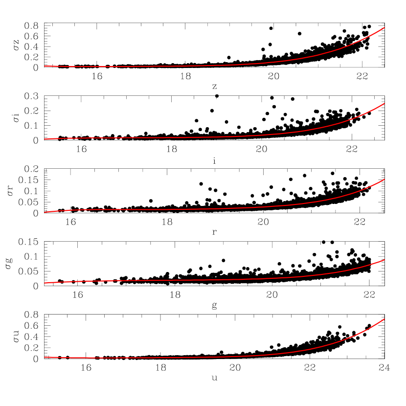
Figure 2: Distribution of photometric errors in the $u$, $g$, $r$, $i$ and $z$ (black dots) passbands, each fitted to a fifth order polynomial (red line).

4.1 Colour and magnitude cuts

The SDSS spectroscopic survey is magnitude-limited. Hence, all our synthetic populations of WD+MS binaries must comply with the magnitude cuts of the SDSS, which are the following ones:

$$15< \,i<19.1\textrm{, for Legacy}$$ (1)

$$15< \,g<22\textrm{, for BOSS}$$ (2)

$$15< \,g<20\textrm{, for SEGUE and SEGUE-2}$$ (3)

Moreover, observed SDSS WD+MS binaries define a clear region in the $ugriz$ colour space (Rebassa-Mansergas et al., 2013) which allows us to define colour cuts to cull our synthetic samples (see Fig. 4 for an example):

$$(u-g)< \,0.93-0.27\times(g-r)-4.7\times(g-r)^{2}+$$

$$\,12.38\times(g-r)^{3}+3.08\times(g-r)^{4}-22.19\times$$

$$\,(g-r)^{5}+16.67\times(g-r)^{6}-3.89\times(g-r)^{7},$$ (4)

$$-0.6<(u-g),$$

$$(g-r)< \,\,2\times(r-i)+0.38\textrm{,\,\,\,\,if }-0.4<(r-i)\leq 0.06,$$

$$(g-r)< \,\,4.5\times(r-i)-0.85\textrm{,\,\,\,\,if }0.3<(r-i)\leq 0.48,$$

$$(g-r)< \,\,0.5\textrm{,\,\,\,\,if }0.06<(r-i)\leq 0.3,$$

$$-0.5<(g-r)<1.3,$$

$$-0.4<(r-i)<1.6,$$

$$(r-i)< \,\,0.5+2\times(i-z)\textrm{,\,\,\,\,if }(i-z)>0,$$

$$(r-i)< \,\,0.5+(i-z)\textrm{,\,\,\,\,if }(i-z)\leq 0,$$

$$-0.8<(i-z)<1.15$$ (5)

It is important to emphasize here that the SEGUE WD+MS binary survey was defined for targeting WD+MS binaries containing cool white dwarfs. Hence, SEGUE WD+MS binaries populate different regions in the $ugriz$ colour space (Rebassa-Mansergas et al., 2012a). These regions define the following colour cuts that we apply to the synthetic SEGUE WD+MS binary population:

$$\,(u-g)<2.25,$$

$$\,-0.2<\, (g-r)<1.2,$$

$$(g-r)>-19.78(r-i)+11.13,$$

$$(g-r)<0.95\times(r-i)+0.5,$$

$$(i-z)>0.5\textrm{,\,\, for }(r-i)>1.0,$$

$$(i-z)>0.68\times(r-i)-0.18\textrm{,\,\, for }(r-i)\leq 1.0,$$

$$\,0.5<\, (r-i)<2.0,$$

$$15\,<\, g<20$$ (6)

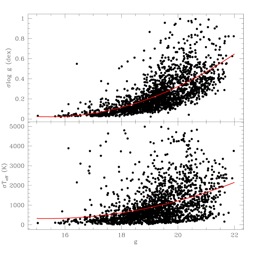
Figure 3: Errors for white dwarf effective temperatures and surface gravities as a function of the apparent magnitude $g$ (black dots), fitted to a third order polynomial distribution (red line).

4.2 Spectroscopic completeness

The target selection criteria employed by the different sub-surveys of the SDSS implies that not all WD+MS binaries have the same probability of being observed. The Legacy and BOSS surveys follow selection criteria that aim at targeting mainly galaxies (Strauss et al., 2002) and quasars (Richards et al., 2002; Ross et al., 2012). Hence, WD+MS binaries containing hot white dwarfs ($>10,000-15,000$ K) and/or late type ($>$M2) companions are more likely to be observed. SEGUE WD+MS binaries are dominated by systems containing cooler white dwarfs and/or early type companions, a simple consequence of the defined target selection criteria (Rebassa-Mansergas et al., 2012a). Finally, SEGUE-2 WD+MS binaries have similar colours to those of single main sequence stars, i.e. the white dwarf contributes little to the spectral energy distribution. Hence, in order to produce realistic simulations of the SDSS WD+MS population we need to implement the probability for a given WD+MS binary to be observed. That is, we need to apply a spectroscopic completeness correction.

The first step in this process is determining the spectroscopic completeness of the observed sample, following the approach described in Camacho et al. (2014). That is, we consider a four dimensional space composed by the $u-g$, $g-r$, $r-i$ and $i-z$ colours, and we define a $0.2$ magnitude four-dimension sphere around each observed source. We then use the casjobs interface to count the number of point sources with clean photometry ($N_{\rm phot}$) as well as the number of spectroscopic sources ($N_{\rm spec}$) within each sphere. The ratio $N_{\rm spec}/N_{\rm phot}$ gives the spectroscopic completeness for the observed system. Then, for each WD+MS binary produced in the synthetic sample, we compute a four-dimensional distance in colour space to each of the observed WD+MS binaries and we select the observed system that is closest to the synthetic one. If the distance to the selected closest observed binary is less than $0.2$ magnitudes, then the synthetic WD+MS pair will be assigned the same spectroscopic completeness as that of the observed one. Conversely, if the distance is larger than $0.2$ magnitudes, then the assigned completeness will be null. This exercise is performed separately for the observed/simulated systems within the four sub-surveys of SDSS.

4.3 Intrinsic WD+MS binary bias

In order to detect in the sample a spectrum of a WD+MS binary the spectral features of both components must be observed. This implies that WD+MS binaries in which one of the two stars dominates the spectral energy distribution will be harder, or even impossible, to detect (Parsons et al., 2016). Moreover, WD+MS binaries that are further away are intrinsically fainter and the resulting SDSS spectra are of lower signal-to-noise ratio (since the SDSS exposures are generally the same for all targets). Identifying the spectral features of the two components is obviously more difficult when dealing with low signal-to-noise ratio spectra. It is then mandatory to eliminate a certain percentage of the synthetic WD+MS binaries according to these reasonings.

Camacho et al. (2014) presented a multi-dimensional grid of WD+MS binary parameters (white dwarf effective temperatures and surface gravities, secondary star spectral types and distances) that allowed to evaluate which synthetic WD+MS binaries would have been detected by the SDSS. In this work we follow the same approach.

Table 1: Percentage of WD+MS binaries respect to the entire sample that survive the observational biases implemented in the simulations. The values are provided for our reference model.

Observational bias	Filtered (%)	Cumulative (%)
Colour and magnitude cuts	$28$	$28$
Spectroscopic completeness	$5$	$1.4$
Intrinsic WD+MS binary bias	$72$	$1.0$

4.4 Uncertainties in the observed parameters

The measured SDSS photometric magnitudes and the stellar parameters derived from fitting the SDSS WD+MS binary spectra can have relatively large uncertainties (Rebassa-Mansergas et al., 2016a). Hence, it is necessary to incorporate such uncertainties in the synthetic WD+MS binary sample before any comparison to the observational data sets is performed. Fig. 2 shows the photometric errors, $\sigma$, as a function of the corresponding magnitude. As can be seen, the photometric errors clearly increase as the apparent magnitude is fainter. We fitted the distributions using fifth order polynomials, that provide us with an expression for $\sigma$ as a function of the apparent magnitude. We then define a Gaussian error distribution for that specific magnitude that we sample in order to obtain the photometric error of each synthetic WD+MS binary in each passband. We apply a similar procedure for the errors in the white dwarf effective temperature and surface gravity, using a third order polynomial fit in this case (see Fig. 3). For the companion spectral type distribution we assumed a constant value of $\sigma$ of one bin, i.e. an uncertainty of one spectral sub-class. Only after adding the corresponding errors in photometric magnitudes and stellar parameters we do apply the colour and magnitude cuts and the other observational filters previously described. Given the random character of this procedure, for each realization providing us with a WD+MS binary sample from the Monte Carlo code, we repeated the process of adding errors and afterwards filtering the sample 20 times per realization.

Table 2: Percentage of present day WD+MS binaries that have undergone common envelope evolution (and have not yet merged), in the complete and filtered sample for different values of $\alpha_{\mathrm{CE}}$ and $\alpha_{\mathrm{int}}$ assumptions. Note that the effect of $\alpha_{\mathrm{int}}$ over the filtered sample becomes negligible.

$\alpha_{\mathrm{CE}}$	$\alpha_{\mathrm{int}}$	Complete sample (%)	Filtered sample (%)
$0.1$	$0.0$	$3$	$10$
$0.2$	$0.0$	$6$	$21$
$0.3$	$0.0$	$10$	$29$
$0.3$	$0.1$	$13$	$30$
$0.3$	$0.2$	$14$	$32$
$0.3$	$0.5$	$17$	$33$
$0.5$	$0.0$	$16$	$38$
$0.7$	$0.0$	$21$	$43$
$1.0$	$0.0$	$26$	$45$

Finally, for both the observed and synthetic samples we only considered systems with a relative error smaller than 10 per cent in effective temperature, and with absolute errors below $0.075$ dex in surface gravity. This explains why different distributions from the same sample contain different numbers of WD+MS pairs.

5 Results

We used our population synthesis code to model the WD+MS binary population in the Galactic disk. For this, we first defined a standard model that uses a flat IMRD ($n(q)$), an age for the thin disk of $10$ Gyr, a constant star formation rate, $\alpha_{\mathrm{CE}}=0.3$, $\alpha_{\mathrm{int}}=0$ and all the fixed parameter assumptions previously explained in Section 3.

5.1 Preliminary checks

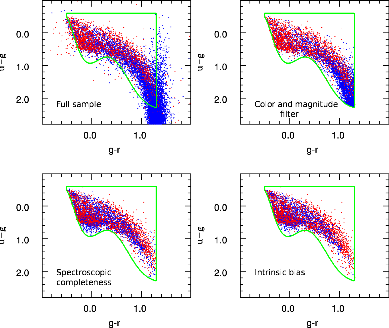
Figure 4: $u-g$ versus $g-r$ colour-colour diagram of the observed (blue dots) and synthetic (red dots) SDSS WD+MS binaries for our reference model, after incorporating the different observational biases explained in Sect. 4. See the on-line version of the journal for a colour version of this figure.

First of all, we analyzed the effects of the observational biases. In Fig. 4 we show a $u-g$ versus $g-r$ colour-colour diagram for the synthetic SDSS WD+MS binary population that results from our reference model (blue dots) compared with the observed sample (red dots). Each panel represents the objects that survive after consecutively applying the filters indicated on it. Starting from the full sample (upper-left panel), we first show the effects of the colour and magnitude filters (upper-right panel), the effects of the spectroscopic completeness bias (lower-left panel) and, finally, the effect of applying the filter for intrinsic bias (lower-right panel). As can be seen in Fig. 4 the number of binaries in the initial synthetic sample decreases dramatically after applying the different colour and magnitude cuts and observational biases. Also, we notice that the final synthetic sample nicely matches the space colour of the observed sample. In order to provide a more quantitative estimate of the effect of the selection criteria, in Table 1 we show the percentage of WD+MS binaries respect to the full sample that survive these filters. The second column represents the percentage with respect the previous applied filter and the third column is the cumulative percentage with respect the initial entire sample. Inspection of the Table 1 reveals that only 1 per cent of the entire simulated WD+MS binary population makes it to the final sample, being the spectroscopic completeness the most restrictive in percentage of the observational biases. These results are in agreement with the analysis of the PCEB sample of Camacho et al. (2014).

In order to properly cover the parameter space, we initially varied several input parameters to better understand their possible effect on the three distributions under scrutiny: the white dwarf effective temperature and surface gravity, and the M dwarf spectral type. We first varied the age of the thin disk between $8$ and $12$ Gyr and realised that the three distributions were not particularly sensitive to this value. We also tried three different prescriptions for the star formation history: a constant rate (used in our reference model), a recent enhanced star formation with one broad peak in the SFR between 1 and 3 Gyr ago (Vergely et al., 2002), and a bimodal SFR with two broad peaks at around 2 and 7 Gyr ago (Rowell, 2013). After testing each of these models independently, we conclude that the choice of the model of star formation has only marginal effects on the synthetic $\log g$ distribution and no other noticeable effect on the other distributions that we analyze.

For convenience, in our simulations we used the IFMR of Hurley et al. (2002), which results from an evolution algorithm consisting basically of a competition between core-mass growth and envelope mass-loss. Nevertheless, we tested this procedure and used the more reliable IFMR of Catalán et al. (2008). We obtained that there is a systematic difference, although the difference of masses of the synthetic white dwarfs is generally not larger than $0.02\,M_{\sun}$.

Lastly, we considered an initial 15 per cent contamination of thick disk stars, which corresponds to a 7-17 per cent contribution to the final sample (after all observational filters are passed), depending on the model parameters. To quantify the effects of the contribution of thick disk systems we ran one simulation in which the contribution of the thick disk was suppressed and we found that the differences distributions were minimal.

5.2 The CE efficiency parameter

The observational analysis of Nebot Gómez-Morán et al. (2011) showed that between 21 and 24 per cent of SDSS WD+MS binaries have experienced a CE phase. In Table 2 we provide, for our reference model, the percentage of present-day WD+MS binaries that have evolved through a CE episode (and did not become semi-detached nor merged) as a function of $\alpha_{\mathrm{CE}}$. We did this for the entire simulated sample and for the restricted (filtered) sample that survives all observational biases outlined in Section 4. Inspection of Table 2 reveals that the percentage of present-day WD+MS binaries that underwent a CE phase is compatible with the observational results of Nebot Gómez-Morán et al. (2011) when $\alpha_{\mathrm{CE}}=0.2-0.3$. For the sake of completeness, we also calculated the percentages assuming different values of $\alpha_{\mathrm{int}}$ (ranging from 0.1 to 0.5). We found that, although we obtain the same $\sim 40$ per cent increase in PCEB systems reported by Zorotovic et al. (2014b) for the complete sample, the results are nearly independent of the adopted value of $\alpha_{\mathrm{int}}$, once the observational filters are applied. Another interesting point would be that observational biases actually favor the discovery of PCEB systems.

An additional way to constrain $\alpha_{\mathrm{CE}}$ is to compare the overall white dwarf $\log g$ distribution of the simulated WD+MS binary population to the observed one. This is done in Fig. 5. By inspecting this figure it becomes clear that $\alpha_{\mathrm{CE}}=0.3$ reproduces best the observational data. This result is in agreement with previous observational studies (Zorotovic et al., 2010) — who found $\alpha_{\mathrm{CE}}=0.2-0.3$ — population synthesis studies of close SDSS WD+MS binaries (Toonen & Nelemans, 2013; Camacho et al., 2014; Zorotovic et al., 2014b) — who found that the CE efficiency should be low — and even with earlier theoretical predictions (Taam2006) — who found $\alpha_{\mathrm{CE}}\leq 0.4-0.5$.

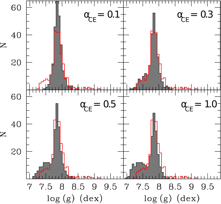
Figure 5: Distribution of white dwarf $\log g$ for different values of $\alpha_{\mathrm{CE}}$ (with $\alpha_{\mathrm{int}}=0$)

Table 3: Our 12 models adopted for the IMRD $n(q)$, ordered from best to worst according to the fit to the observational $T_{\mathrm{eff}}$ distributions, the value of the three distance metrics used in our analysis being averaged between the results for the Legacy survey, for the BOSS survey and for the overall distribution (see text for details).

Model	$\langle D_{\rm KL}\rangle$	Model	$\langle D_{\rm LS}\rangle$	Model	$\langle{\beta}\rangle\,(^{\circ})$
$3$	$4.8\times 10^{-2}$	$3$	$4.9\times 10^{-3}$	$3$	$8.7$
$4$	$4.8\times 10^{-2}$	$4$	$6.0\times 10^{-3}$	$6$	$9.2$
$6$	$5.0\times 10^{-2}$	$6$	$6.0\times 10^{-3}$	$4$	$10.0$
$5$	$5.4\times 10^{-2}$	$1$	$6.1\times 10^{-3}$	$5$	$10.2$
$1$	$5.8\times 10^{-2}$	$5$	$6.3\times 10^{-3}$	$1$	$10.8$
$7$	$6.5\times 10^{-2}$	$7$	$8.1\times 10^{-3}$	$7$	$12.2$
$2$	$7.7\times 10^{-2}$	$12$	$1.5\times 10^{-2}$	$12$	$14.3$
$12$	$7.9\times 10^{-2}$	$2$	$1.5\times 10^{-2}$	$2$	$14.5$
$8$	$1.1\times 10^{-1}$	$8$	$2.5\times 10^{-2}$	$8$	$18.1$
$9$	$1.2\times 10^{-1}$	$9$	$2.7\times 10^{-2}$	$9$	$18.8$
$10$	$1.6\times 10^{-1}$	$10$	$3.6\times 10^{-2}$	$10$	$21.8$
$11$	$2.4\times 10^{-1}$	$11$	$4.0\times 10^{-2}$	$11$	$23.1$

Table 4: Same as Table 3, but using the $\log g$ distributions.

Model	$\langle D_{\rm KL}\rangle$	Model	$\langle D_{\rm LS}\rangle$	Model	$\langle{\beta}\rangle\,(^{\circ})$
$5$	$2.4\times 10^{-1}$	$4$	$9.0\times 10^{-3}$	$6$	$17.9$
$3$	$2.4\times 10^{-1}$	$3$	$9.0\times 10^{-3}$	$5$	$18.1$
$6$	$2.5\times 10^{-1}$	$5$	$1.0\times 10^{-2}$	$4$	$18.4$
$4$	$2.6\times 10^{-1}$	$1$	$1.2\times 10^{-2}$	$3$	$18.6$
$1$	$2.7\times 10^{-1}$	$6$	$1.2\times 10^{-2}$	$1$	$18.7$
$7$	$2.8\times 10^{-1}$	$7$	$1.4\times 10^{-2}$	$7$	$19.3$
$8$	$3.3\times 10^{-1}$	$12$	$1.7\times 10^{-2}$	$8$	$21.7$
$2$	$4.4\times 10^{-1}$	$2$	$1.8\times 10^{-2}$	$2$	$21.7$
$12$	$4.8\times 10^{-1}$	$9$	$2.0\times 10^{-2}$	$12$	$23.0$
$11$	$6.3\times 10^{-1}$	$8$	$2.2\times 10^{-2}$	$9$	$24.7$
$9$	$6.4\times 10^{-1}$	$11$	$3.8\times 10^{-2}$	$11$	$27.0$
$10$	$1.1\times 10^{0}$	$10$	$4.2\times 10^{-2}$	$10$	$32.6$

Table 5: Same as Table 3, but using the M dwarf spectral type distributions. The first five models fit best the observational data, the last seven models can be excluded. The seven IMRD dstributions that can be excluded all increase with $q$.

Model	$\langle D_{\rm KL}\rangle$	Model	$\langle D_{\rm LS}\rangle$	Model	$\langle{\beta}\rangle\,(^{\circ})$
$6$	$2.2\times 10^{-2}$	$6$	$8.3\times 10^{-3}$	$6$	$8.3$
$3$	$2.3\times 10^{-2}$	$3$	$1.1\times 10^{-2}$	$3$	$9.2$
$5$	$4.8\times 10^{-2}$	$5$	$2.0\times 10^{-2}$	$5$	$13.2$
$4$	$5.0\times 10^{-2}$	$4$	$2.1\times 10^{-2}$	$4$	$13.5$
$1$	$5.1\times 10^{-2}$	$1$	$2.2\times 10^{-2}$	$1$	$13.5$
$7$	$8.1\times 10^{-2}$	$7$	$3.1\times 10^{-2}$	$7$	$16.8$
$2$	$2.0\times 10^{-1}$	$2$	$5.7\times 10^{-2}$	$2$	$22.7$
$12$	$2.8\times 10^{-1}$	$12$	$6.3\times 10^{-2}$	$12$	$24.7$
$10$	$8.2\times 10^{-1}$	$10$	$1.1\times 10^{-1}$	$10$	$35.2$
$8$	$9.3\times 10^{-1}$	$8$	$1.3\times 10^{-1}$	$8$	$37.6$
$9$	$1.1\times 10^{0}$	$9$	$1.6\times 10^{-1}$	$9$	$39.4$
$10$	$1.2\times 10^{0}$	$11$	$1.8\times 10^{-1}$	$11$	$41.7$

5.3 The initial mass ratio distribution

Our Monte Carlo simulator, calibrated using the largest sample of SDSS WD+MS binaries currently known (Rebassa-Mansergas et al., 2016a) and taking into account all known observational biases, offers us an excellent opportunity to constrain the properties of the IMRD, $n(q)$. Hereafter we define the mass ratio as $q=m_{2}/m_{1}$, where $m_{1}$ is the mass of the primary (or more massive) star in a main sequence binary, and $m_{2}$ is the mass of its main sequence companion or secondary star. The IMRD is an important tool for understanding the evolution of stars in binary systems and for constraining models of binary star formation. The precise shape of the IMRD has been a topic of much debate for over four decades, with results often contradicting each other. Indeed, decreasing (Jaschek & Ferrer, 1972), increasing (Dabbowski & Beardsley, 1977), bimodal (Trimble, 1974) and flat (Raghavan et al., 2010) IMRDs have been suggested. This lack of agreement remains when recent results are considered. For example, whilst Ducati et al. (2011) claim that the IMRD decreases as $q$ increases, Reggiani & Meyer (2013) suggest a slowly increasing IMRD. These discrepancies may be a simple consequence of the IMRD being dependent on both the primary mass and the orbital separation, as suggested by Duchêne & Kraus (2013). This seems to be confirmed by several observational studies (Carrier et al., 2002; Burgasser et al., 2006; Delfosse et al., 2004; Carquillat & Prieur, 2007; Raghavan et al., 2010; Tokovinin, 2011; Sana et al., 2012; Reggiani & Meyer, 2013; Gullikson et al., 2016). However, it is important to emphasize that these observational studies are affected by important selection effects, which likely introduce sizable uncertainties in the results. This is particularly important when the secondary star in a main sequence binary is intrinsically faint and thus harder to detect against a moderately hot primary.

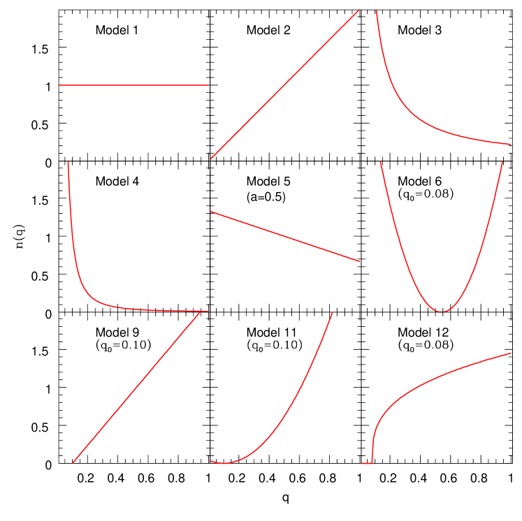
Figure 6: The 12 IMRD adopted in our simulations. Note that the only difference between models 6–7, 8–9 and 10–11 are the assumed values of $q_{0}$ ($0.08$ or $0.1$), hence we only display one of them. The distributions have been normalized to unity.

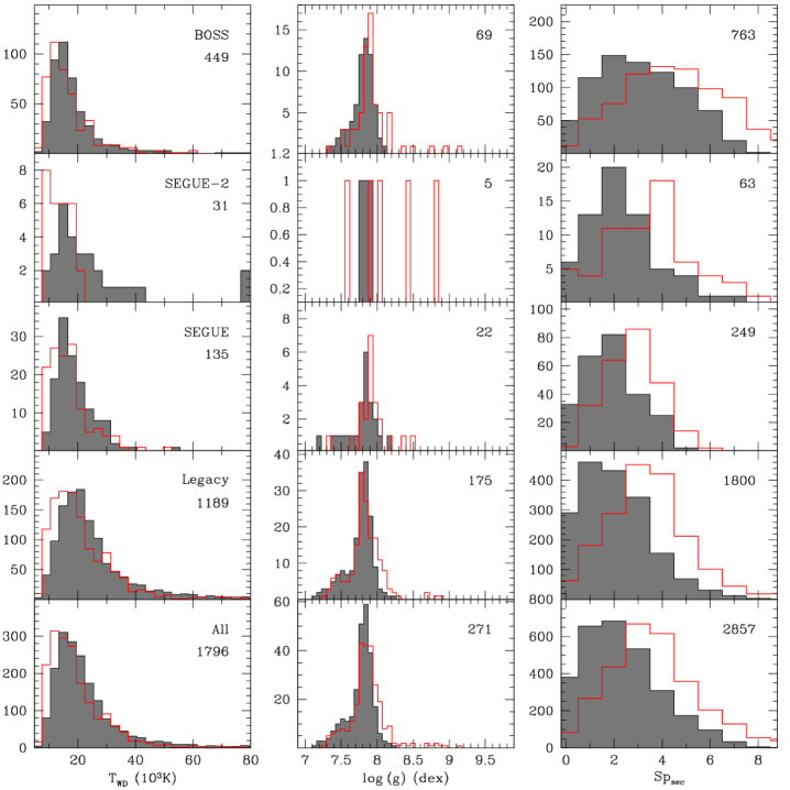
Figure 7: White dwarf effective temperature, surface gravity and M dwarf spectral type distributions. Observational data from Rebassa-Mansergas et al. (2016a) (gray histograms), synthetic data obtained assuming a $n(q)\sim q$ (red open histograms). These panels display an example of a bad fit.

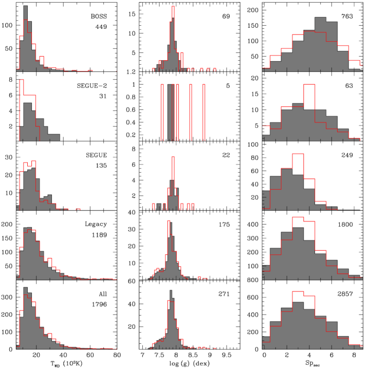
Figure 8: White dwarf effective temperature, surface gravity and M dwarf spectral type distributions. Observational data from Rebassa-Mansergas et al. (2016a) (gray histograms), synthetic data obtained assuming a $n(q)\sim q^{-1}$ (red open histograms). These panels show an example of a good fit.

Recently, Ducati et al. (2011) compared the results of a set of Monte Carlo simulations of a large number of models with different IMRDs with a sample of 249 binaries belonging to the Ninth Catalogue of Spectroscopic Binaries (Pourbaix et al., 2004). Their findings favor a linearly decreasing $n(q)\sim 1-aq$, with $a=0.5$. However, given the diversity of the models they studied, we adopt most of them together with the more classical IMRD studied in Camacho et al. (2014), testing in total $12$ models for the IMRD. We first adopted the three most frequently assumed IMRDs. In particular, our first model corresponds to $n(q)\propto 1$ (model 1). Hence for model 1 we use a flat distribution, which will be regarded as the reference model. Next we also used two frequently employed IMRDs, namely $n(q)\propto q$ (model 2) and $n(q)\propto q^{-1}$ (model 3). The other six models that we used are less frequently employed, and are the following ones. Model 4 corresponds to $n(q)\propto q^{-2}$ (Hogeveen, 1992). Model 5 is the best model of Ducati et al. (2011) $n(q)\propto 1-a\,q$, being $a=0.5$. For models 6 and 7 we adopted $n(q)\propto\left(q-\left(1+q_{0}\right)/2\right)^{2}$, with $q_{0}=0.08$ and $q_{0}=0.10$, respectively. These models are inspired in the bimodal distributions of Trimble (1974). In models 8 and 9 we used $n(q)\propto q-q_{0}$ with $q_{0}=0.08$ and $q_{0}=0.10$, whereas for models 10 and 11 the dependence on $q$ is steeper $n(q)\propto(q-q_{0})^{2}$, with $q_{0}=0.08$ and $q_{0}=0.10$, respectively. These models peak at $q=1.0$, as in the data of Fisher et al. 2005. Finally, the IMRD of model 12 is based on the findings of Reggiani & Meyer (2013), $n(q)\propto(q-q_{0})^{1/3}$, with $q_{0}=0.08$. In Fig. 6 we display the 12 IMRDs.

The best approach for comparing the simulated distributions to the observed ones is to use distance metrics, a procedure which will allow us not only to decide which simulated distribution fits best the observed data, but also to order the models from best to worst. Among the possible number of distance metrics that can be defined, we chose three commonly employed ones. Let $P$ be the observed distribution and $Q$ the simulated one, the three metrics employed here are the following ones. We first employed a standard least squares method:

$$D_{\rm LS}=\sum_{i}(P(i)-Q(i))^{2}$$ (7)

We also used the so-called Kullback-Leibler (KL) divergence:

$$D_{\rm KL}=\sum_{i}P(i)\ln\left(\frac{P(i)}{Q(i)}\right)$$ (8)

Finally, we employed a less known method, the so-called Bhattacharyya coefficient:

$$\cos(\beta)=\sum_{i}\sqrt{P(i)Q(i)}$$ (9)

The least squares method is a standard distance metric. On the other hand, the Kullback-Leibler divergence is not symmetrical and both this distance metric and the Bhattacharyya coefficient do not satisfy the triangle inequality, thus they must be considered pre-metrics. The Bhattacharyya coefficient also has an interesting geometrical interpretation, as the cosine of the angle between two multidimensional vectors describing the two distributions.

We employed these three methods and ordered the models from lowest to largest distance (or angle), using the $T_{\rm eff}$ and $\log\,g$ distributions for the white dwarf and the spectral type distribution of the M dwarf, from Legacy and BOSS data and also the overall distributions. We did not use SEGUE and SEGUE-2 data because the sample sizes are small. The overall results are shown in an ordered way in Tables 3, 4 and 5.

Inspection of Tables 3, 4 and 5 reveals that we roughly obtain the same order (from best to worst model) independently of which one of the three metrics is used. These types of distance metrics are generally used in optimizations and it is well known that the order they give is reliable. However, they cannot be used to assess which model truly offers a good fit — that is, which models reproduce the observed distribution — and which do not. In order to further understand and quantify this issue we performed the following test. We computed the angle which defines the Bhattacharyya coefficient between two distributions sampled from the same model — that is, the same parameter set — using a different initial random seed. We found that typically we obtain a value of $\beta$ ranging from $7$ to $10^{\circ}$ (on average $8.5^{\circ}$) for the distributions of $T_{\mathrm{eff}}$, between $11$ and $17^{\circ}$ (with a mean of $14^{\circ}$) for the distributions of $\log g$, and between $3$ and $6^{\circ}$ (with an average value of $4.5^{\circ}$) for the M-dwarf spectral type distribution.

Keeping the average values of $\beta$ in mind and comparing them to the angles listed in Tables 3 and 4 for the $T_{\rm eff}$ and $\log g$ distributions, it can be easily realized that for most models the angles between the theoretical distributions and the observed data are smaller than 2 times the average values. Conversely, in Table 5, which gives the angles between the M-dwarf spectral type distributions, it can be seen that only two of the 12 models are within an angle smaller than 2 times the mean angle. This clearly indicates that the M dwarf spectral type distribution is much more sensitive to the choice of the IMRD. We thus set a threshold of 3 times the average angle for the M-dwarf spectral type distributions (i.e. $13.5^{\circ}$) below which we consider the IMRDs to be representative of the observed data. Interestingly, under this assumption, we can exclude the seven IMRDs with increasing slopes (see Table 5 and Fig. 6). In order to exemplify this, we show in Fig. 7 and Fig. 8 a poor and a good fit to the observed data. It is also worth mentioning that the minimum value of $0.08$ for the minimal mass ratio parameter $q_{0}$ generally performs better. Finally, among all IMRDs that satisfy that the angle between the theoretical distribution and the observed data is smaller than 13.5 we find both our reference model ($n(q)=1$) and the most favored model of Ducati et al. (2011).

We also investigated the possible correlations between the IMRD and the $\alpha_{\mathrm{CE}}$ parameters by varying $\alpha_{\mathrm{CE}}$ from 0.0 to 0.5 for three representative IMRD models: model 1 (flat), model 2 (linearly increasing) and model 3 (inversely decreasing). For each of these three IMRDs we find that the white dwarf effective temperature distributions and the secondary spectral type distributions are largely unaffected by the increase in $\alpha_{\mathrm{CE}}$. Moreover, the $\log g$ distribution shows the same behaviour described in Section 5.2 (see also Fig. 5) relative to the increase of $\alpha_{\mathrm{CE}}$, irrespective of the considered IMRD.

6 Conclusions

We have presented the most detailed population synthesis study to date of the WD+MS binary population in the Galactic disk. In particular, our work aimed at reproducing the ensemble properties of the population of such binaries in the SDSS data release 12. To do so we have independently simulated the different WD+MS binary sub-populations observed by the Legacy, BOSS, SEGUE and SEGUE-2 surveys of the SDSS, taking special care in implementing all observational biases known for each one of them.

We have found that a value of the common envelope efficiency parameter between 0.2 and 0.3 is compatible with the observational data. This is true not only in terms of the percentage of WD+MS binaries that experienced a common envelope episode, but also regarding the overall properties of the distributions of white dwarf effective temperatures and surface gravities. This result is consistent with previous observational (Zorotovic et al., 2010) and population synthesis (Toonen & Nelemans, 2013; Camacho et al., 2014; Zorotovic et al., 2014b) analyses of the population of close SDSS WD+MS binaries.

Moreover, we have adopted 12 different prescriptions for the initial mass ratio distribution of main sequence binaries, which include a wide variety of shapes. We have used three distance metric indicators to compare the resulting synthetic M-dwarf spectral type and white dwarf effective temperature and surface gravity distributions with their observed counterparts. Our results indicate that all initial mass ratio distributions of ascending shape can be excluded.

Finally, it is worth mentioning that the outcome of the simulations is nearly independent on the age of the thin disk (up to a 20 per cent variation), on the contribution of WD+MS binaries from the thick disk and on the fraction of the internal energy that is used to eject the envelope during the common envelope episode. All these findings are important by themselves and open the possibility of using the population of binary systems composed of a white dwarf and main sequence star to probe the structure and evolution of our Galaxy, and also to elucidate between different models aimed at reproducing the evolution of binary stars.

References

- Abazajian et al. (2009) Abazajian K. N., et al., 2009, ApJS, 182, 543
- Adelman-McCarthy et al. (2008) Adelman-McCarthy J. K., et al., 2008, ApJS, 175, 297
- Ak et al. (2013) Ak T., Bilir S., Güver T., Çakmak H., Ak S., 2013, New Astron., 22, 7
- Althaus et al. (2005) Althaus L. G., García-Berro E., Isern J., Córsico A. H., 2005, A&A, 441, 689
- Althaus et al. (2007) Althaus L. G., García-Berro E., Isern J., Córsico A. H., Rohrmann R. D., 2007, A&A, 465, 249
- Baraffe et al. (2015) Baraffe I., Homeier D., Allard F., Chabrier G., 2015, A&A, 577, A42
- Bland-Hawthorn & Gerhard (2016) Bland-Hawthorn J., Gerhard O., 2016, Annual Review of Astronomy and Astrophysics, 54, null
- Burgasser et al. (2006) Burgasser A. J., Kirkpatrick J. D., Cruz K. L., Reid I. N., Leggett S. K., Liebert J., Burrows A., Brown M. E., 2006, ApJS, 166, 585
- Camacho et al. (2014) Camacho J., Torres S., García-Berro E., Zorotovic M., Schreiber M. R., Rebassa-Mansergas A., Nebot Gómez-Morán A., Gänsicke B. T., 2014, A&A, 566, A86
- Carquillat & Prieur (2007) Carquillat J.-M., Prieur J.-L., 2007, MNRAS, 380, 1064
- Carrier et al. (2002) Carrier F., North P., Udry S., Babel J., 2002, A&A, 394, 151
- Catalán et al. (2008) Catalán S., Isern J., García-Berro E., Ribas I., 2008, MNRAS, 387, 1693
- Claeys et al. (2014) Claeys J. S. W., Pols O. R., Izzard R. G., Vink J., Verbunt F. W. M., 2014, A&A, 563, A83
- Cojocaru et al. (2014) Cojocaru R., Torres S., Isern J., García-Berro E., 2014, A&A, 566, A81
- Dabbowski & Beardsley (1977) Dabbowski J. P., Beardsley W. R., 1977, PASP, 89, 225
- Davis et al. (2010) Davis P. J., Kolb U., Willems B., 2010, MNRAS, 403, 179
- Dawson et al. (2013) Dawson K. S., et al., 2013, AJ, 145, 10
- De Marco et al. (2011) De Marco O., Passy J.-C., Moe M., Herwig F., Mac Low M.-M., Paxton B., 2011, MNRAS, 411, 2277
- Delfosse et al. (2004) Delfosse X., et al., 2004, in Hilditch R. W., Hensberge H., Pavlovski K., eds, Astronomical Society of the Pacific Conference Series Vol. 318, Spectroscopically and Spatially Resolving the Components of the Close Binary Stars. pp 166–174
- Ducati et al. (2011) Ducati J. R., Penteado E. M., Turcati R., 2011, A&A, 525, A26
- Duchêne & Kraus (2013) Duchêne G., Kraus A., 2013, ARA&A, 51, 269
- Dye et al. (2006) Dye S., et al., 2006, MNRAS, 372, 1227
- Feltzing & Bensby (2009) Feltzing S., Bensby T., 2009, in Mamajek E. E., Soderblom D. R., Wyse R. F. G., eds, IAU Symposium Vol. 258, The Ages of Stars. pp 23–30
- Ferrario (2012) Ferrario L., 2012, MNRAS, 426, 2500
- Fisher et al. (2005) Fisher J., Schröder K.-P., Smith R. C., 2005, MNRAS, 361, 495
- García-Berro et al. (1999) García-Berro E. Torres S., Isern J., Burkert A., 1999, MNRAS, 302, 173
- García-Berro et al. (2004) García-Berro E., Torres S., Isern J., Burkert A., 2004, A&A, 418, 53
- Gullikson et al. (2016) Gullikson K., Kraus A., Dodson-Robinson S., 2016, AJ, 152, 40
- Hakkila et al. (1997) Hakkila J., Myers J. M., Stidham B. J., Hartmann D. H., 1997, AJ, 114, 2043
- Han et al. (1995) Han Z., Podsiadlowski P., Eggleton P. P., 1995, MNRAS, 272, 800
- Heggie (1975) Heggie D. C., 1975, MNRAS, 173, 729
- Heller et al. (2009) Heller R., Homeier D., Dreizler S., Østensen R., 2009, A&A, 496, 191
- Hogeveen (1992) Hogeveen S. J., 1992, Ap&SS, 196, 299
- Holmberg & Flynn (2000) Holmberg J., Flynn C., 2000, MNRAS, 313, 209
- Hurley et al. (2002) Hurley J. R., Tout C. A., Pols O. R., 2002, MNRAS, 329, 897
- Jaschek & Ferrer (1972) Jaschek C., Ferrer O., 1972, PASP, 84, 292
- Jordi et al. (2006) Jordi K., Grebel E. K., Ammon K., 2006, A&A, 460, 339
- Kilic et al. (2014) Kilic M., Brown W. R., Gianninas A., Hermes J. J., Allende Prieto C., Kenyon S. J., 2014, MNRAS, 444, L1
- Kroupa (2001) Kroupa P., 2001, MNRAS, 322, 231
- Liu et al. (2012) Liu C., Li L., Zhang F., Zhang Y., Jiang D., Liu J., 2012, MNRAS, 424, 1841
- Marsh et al. (2014) Marsh T. R., et al., 2014, MNRAS, 437, 475
- Nebot Gómez-Morán et al. (2009) Nebot Gómez-Morán A., et al., 2009, A&A, 495, 561
- Nebot Gómez-Morán et al. (2011) Nebot Gómez-Morán A., et al., 2011, A&A, 536, A43
- Parsons et al. (2013) Parsons S. G., et al., 2013, MNRAS, 429, 256
- Parsons et al. (2015) Parsons S. G., et al., 2015, MNRAS, 449, 2194
- Parsons et al. (2016) Parsons S. G., Rebassa-Mansergas A., Schreiber M. R., Gänsicke B. T., Zorotovic M., Ren J. J., 2016, MNRAS, 463, 2125
- Pickles (1998) Pickles A. J., 1998, PASP, 110, 863
- Pols et al. (1998) Pols O. R., Schröder K.-P., Hurley J. R., Tout C. A., Eggleton P. P., 1998, MNRAS, 298, 525
- Pourbaix et al. (2004) Pourbaix D., et al., 2004, A&A, 424, 727
- Pyrzas et al. (2009) Pyrzas S., et al., 2009, MNRAS, 394, 978
- Raghavan et al. (2010) Raghavan D., et al., 2010, ApJS, 190, 1
- Rebassa-Mansergas et al. (2007) Rebassa-Mansergas A., Gänsicke B. T., Rodríguez-Gil P., Schreiber M. R., Koester D., 2007, MNRAS, 382, 1377
- Rebassa-Mansergas et al. (2010) Rebassa-Mansergas A., Gänsicke B. T., Schreiber M. R., Koester D., Rodríguez-Gil P., 2010, MNRAS, 402, 620
- Rebassa-Mansergas et al. (2011) Rebassa-Mansergas A., Nebot Gómez-Morán A., Schreiber M. R., Girven J., Gänsicke B. T., 2011, MNRAS, 413, 1121
- Rebassa-Mansergas et al. (2012a) Rebassa-Mansergas A., Nebot Gómez-Morán A., Schreiber M. R., Gänsicke B. T., Schwope A., Gallardo J., Koester D., 2012a, MNRAS, 419, 806
- Rebassa-Mansergas et al. (2012b) Rebassa-Mansergas A., et al., 2012b, MNRAS, 423, 320
- Rebassa-Mansergas et al. (2013) Rebassa-Mansergas A., Agurto-Gangas C., Schreiber M. R., Gänsicke B. T., Koester D., 2013, MNRAS, 433, 3398
- Rebassa-Mansergas et al. (2016a) Rebassa-Mansergas A., Ren J. J., Parsons S. G., Gänsicke B. T., Schreiber M. R., García-Berro E., Liu X.-W., Koester D., 2016a, MNRAS, 458, 3808
- Rebassa-Mansergas et al. (2016b) Rebassa-Mansergas A., et al., 2016b, MNRAS, 463, 1137
- Reggiani & Meyer (2013) Reggiani M., Meyer M. R., 2013, A&A, 553, A124
- Reid (2005) Reid I. N., 2005, ARA&A, 43, 247
- Ren et al. (2014) Ren J. J., et al., 2014, A&A, 570, A107
- Renedo et al. (2010) Renedo I., Althaus L. G., Miller Bertolami M. M., Romero A. D., Córsico A. H., Rohrmann R. D., García-Berro E., 2010, ApJ, 717, 183
- Richards et al. (2002) Richards G. T., et al., 2002, AJ, 123, 2945
- Ross et al. (2012) Ross N. P., et al., 2012, ApJS, 199, 3
- Rowell (2013) Rowell N., 2013, MNRAS, 434, 1549
- Rowell & Hambly (2011) Rowell N., Hambly N. C., 2011, MNRAS, 417, 93
- Sana et al. (2012) Sana H., et al., 2012, Science, 337, 444
- Schlafly et al. (2010) Schlafly E. F., Finkbeiner D. P., Schlegel D. J., Jurić M., Ivezić Ž., Gibson R. R., Knapp G. R., Weaver B. A., 2010, ApJ, 725, 1175
- Schreiber et al. (2010) Schreiber M. R., et al., 2010, A&A, 513, L7
- Serenelli et al. (2001) Serenelli A. M., Althaus L. G., Rohrmann R. D., Benvenuto O. G., 2001, MNRAS, 325, 607
- Smolčić et al. (2004) Smolčić V., et al., 2004, ApJ, 615, L141
- Strauss et al. (2002) Strauss M. A., et al., 2002, AJ, 124, 1810
- Taam & Ricker (2006) Taam, R. E., & Ricker, P. M. 2006, arXiv:astro-ph/0611043
- Tokovinin (2011) Tokovinin A., 2011, AJ, 141, 52
- Toonen & Nelemans (2013) Toonen S., Nelemans G., 2013, A&A, 557, A87
- Torres et al. (2005) Torres S., García-Berro E., Isern J., Figueras F., 2005, MNRAS, 360, 1381
- Tout et al. (1997) Tout C. A., Aarseth S. J., Pols O. R., Eggleton P. P., 1997, MNRAS, 291, 732
- Trimble (1974) Trimble V., 1974, AJ, 79, 967
- Vergely et al. (2002) Vergely J.-L., Lançon A., Mouhcine 2002, A&A, 394, 807
- Webbink (2008) Webbink R. F., 2008, in Milone E. F., Leahy D. A., Hobill D. W., eds, Astrophysics and Space Science Library Vol. 352, Astrophysics and Space Science Library. p. 233
- Willems & Kolb (2004) Willems B., Kolb U., 2004, A&A, 419, 1057
- Yanny et al. (2009) Yanny B., et al., 2009, AJ, 137, 4377
- York et al. (2000) York D. G., et al., 2000, AJ, 120, 1579
- Zhao et al. (2012) Zhao G., Zhao Y.-H., Chu Y.-Q., Jing Y.-P., Deng L.-C., 2012, Research in Astronomy and Astrophysics, 12, 723
- Zorotovic & Schreiber (2013) Zorotovic M., Schreiber M. R., 2013, A&A, 549, A95
- Zorotovic et al. (2010) Zorotovic M., Schreiber M. R., Gänsicke B. T., Nebot Gómez-Morán A., 2010, A&A, 520, A86
- Zorotovic et al. (2011) Zorotovic M., et al., 2011, A&A, 536, L3
- Zorotovic et al. (2014a) Zorotovic M., Schreiber M. R., Parsons S. G., 2014a, A&A, 568, L9
- Zorotovic et al. (2014b) Zorotovic M., Schreiber M. R., García-Berro E., Camacho J., Torres S., Rebassa-Mansergas A., Gänsicke B. T., 2014b, A&A, 568, A68
- Zorotovic et al. (2016) Zorotovic M., et al., 2016, MNRAS, 457, 3867