New method of computing the contributions of graphs without lepton loops to the electron anomalous magnetic moment in QED

This paper presents a new method of numerical computation of the mass-independent QED contributions to the electron anomalous magnetic moment which arise from Feynman graphs without closed electron loops. The method is based on a forest-like subtraction formula that removes all ultraviolet and infrared divergences in each Feynman graph before integration in Feynman-parametric space. The integration is performed by an importance sampling Monte-Carlo algorithm with the probability density function that is constructed for each Feynman graph individually. The method is fully automated at any order of the perturbation series. The results of applying the method to 2-loop, 3-loop, 4-loop Feynman graphs, and to some individual 5-loop graphs are presented, as well as the comparison of this method with other ones with respect to Monte Carlo convergence speed.

I INTRODUCTION

The electron anomalous magnetic moment (AMM) is known with a very high precision. In the experiment [1] the value

$$a_{e}=0.00115965218073(28)$$

was obtained. So, an extremely high accuracy is needed also from theoretical predictions.

The most precise prediction of electron’s AMM at the present time  [2] has the following representation:

$$a_{e}=a_{e}(\text{QED})+a_{e}(\text{hadronic})+a_{e}(\text{electroweak}),$$

$$a_{e}(\text{QED})=\sum_{n\geq 1}\left(\frac{\alpha}{\pi}\right)^{n}a_{e}^{2n},$$

$$a_{e}^{2n}=A_{1}^{(2n)}+A_{2}^{(2n)}(m_{e}/m_{\mu})+A_{2}^{(2n)}(m_{e}/m_{\tau})+A_{3}^{(2n)}(m_{e}/m_{\mu},m_{e}/m_{\tau}),$$

where $m_{e}$, $m_{\mu}$, $m_{\tau}$ are masses of electron, muon, and tau lepton, respectively. The corresponding numerical value

$$a_{e}=0.001159652181643(25)(23)(16)(763)$$ (1)

was obtained by using the fine structure constant $\alpha^{-1}=137.035999049(90)$ that had been measured in the recent experiments with rubidium atoms (see  [3, 4]). Here, the first, second, third, and fourth uncertainties come from $A_{1}^{(8)}$, $A_{1}^{(10)}$, $a_{e}(\text{hadronic})+a_{e}(\text{electroweak})$ and the fine-structure constant respectively. Thus, a still relevant problem is to compute $A_{1}^{(2n)}$ with a maximum possible accuracy. The values

$$A^{(2)}_{1}=0.5,$$

$$A_{1}^{(4)}=-0.328478965579193\ldots,$$

$$A_{1}^{(6)}=1.181241456\ldots$$

are known from the analytical results in  [5, 6],  [7, 8],  [9], respectively. The values

$$A_{1}^{(8)}=-1.91298(84),\quad A_{1}^{(10)}=7.795(336).$$

were presented by T.Kinoshita et al. in  [2]. The first one was recently confirmed and improved by S.Laporta using semi-analytical computation  [21]:

$$A_{1}^{(8)}=-1.9122457649\ldots.$$

Thus, the precision of (1) can be slightly improved. At the present time, there are no independent calculations of $A_{1}^{(10)}$.

This paper presents a method of computing the contribution of Feynman graphs without lepton loops to $A_{1}^{(2n)}$. We denote this contribution by $A_{1}^{(2n)}[\text{no lepton loops}]$. The method consists of two parts: the subtraction procedure for removal of UV and IR divergences in Feynman-parametric space before integration and the graph-specific importance sampling Monte Carlo integration.

The subtraction procedure was presented in  [22]. It is briefly described in Section II.C. This procedure eliminates IR and UV divergences in each AMM Feynman graph point-by-point, before integration, in the spirit of papers  [2, 23, 24, 25, 26, 27, 28, 29, 31, 30, 32, 33] etc. This property is substantial for many-loop calculations when reducing an amount of the needed computer resources is of critical importance. Let us remark that $A_{1}^{(2n)}$ is free from infrared divergences since they are removed by the on-shell renormalization as well as the ultraviolet ones (see a more detailed explanation in  [22]). However, the standard subtractive on-shell renormalization can’t remove IR divergences in Feynman-parametric space before integration as well as it does for UV divergences. The structure of IR and UV divergences in individual Feynman graphs is quite complicated. IR and UV divergences can be, in a certain sense, entangled with each other. Therefore, a special procedure is required for removing both UV and IR divergences. Let us recapitulate the advantages of the developed subtraction procedure.

1. It is fully automated for any $n$.

2. It is comparatively easy for realization on computers.

3. It can be represented as a forest-like formula. This formula differs from the forest formula of Zavialov and Stepanov [31], Scherbina [30], and Zimmermann [37] only in the choice of linear operators and in the way of combining them.

4. The contribution of each Feynman graph to $A_{1}^{(2n)}$ can be represented as a single Feynman-parametric integral. The value of $A_{1}^{(2n)}$ is the sum of these contributions.

5. Feynman parameters can be used directly, without any additional tricks.

See a detailed description in  [22]. The subtraction procedure was checked independently by F. Rappl using Monte Carlo integration based on Markov chains  [38].

All Feynman-parametric integrals are finite after applying the subtraction procedure. However, the integrands remain badly-behaved: they have a steep landscape, peaks and integrable singularities. This fact makes it difficult to integrate with a high accuracy when the number of dimensions is large (for example, for $n=5$ we have $13$ dimensions or even more). The known universal integration routines can solve this problem only partially and often not satisfactorily. However, the simplicity of the subtraction procedure makes it possible to understand the behaviour of integrands and to develop an importance sampling Monte Carlo algorithm based on this known behaviour. The algorithm for the integrands corresponding to AMM Feynman graphs without lepton loops is presented in Section III. This algorithm is based on the ideas that were used by different scientists for proving UV-finiteness of renormalized Feynman amplitudes  [39, 40]. The probability density function is constructed for each Feynman graph individually. For constructing the probability density function we use the ultraviolet degrees of divergence of the so-called I-closures of sets of graph internal lines. The notion of I-closure is first introduced in this paper. It was observed that the behaviour of on-shell Feynman-parametric integrands is well approximated using I-closures. The developed importance sampling integration can be combined with splitting-based adaptive algorithms. A variant of an adaptive algorithm is provided (see Section IV.A). The new integration algorithm has the following advantages:

• fast convergence

• reliable error estimation on early stages of calculation

• relatively small part of samples requires increased arithmetic precision for preventing round-off errors (compared to the method from  [22], for example)

The techniques for stabilizing and for preventing error underestimation are presented (Section III.D). This Monte Carlo algorithm can also be used for integrating other Feynman-parametric integrals provided that we have the needed information about the integrand behaviour.

Numerical calculation results that were obtained on a personal computer are presented in Section IV: $A_{1}^{(2n)}[\text{no lepton loops}]$ for $n=2,3,4$, the contrubutions of the ladder graphs and the fully crossed ladder graphs up to 5 loops. Each value is given with the error estimation and with the number of Monte Carlo samples. The comparison of this results with known ones with respect to values (Section IV.B) and Monte Carlo convergence speed (Section IV.C) is presented. The results for the 4-loop and 5-loop fully crossed ladder graphs are new.

II CONSTRUCTION OF THE INTEGRANDS

A Preliminary remarks

We will work in the system of units, in which $\hbar=c=1$, the factors of $4\pi$ appear in the fine-structure constant: $\alpha=e^{2}/(4\pi)$, the tensor $g_{\mu\nu}$ is defined by

$$g_{\mu\nu}=g^{\mu\nu}=\left(\begin{matrix}1&0&0&0\\ 0&-1&0&0\\ 0&0&-1&0\\ 0&0&0&-1\end{matrix}\right),$$

the Dirac gamma-matrices satisfy the following condition $\gamma^{\mu}\gamma^{\nu}+\gamma^{\nu}\gamma^{\mu}=2g^{\mu\nu}$.

We will use Feynman graphs with the propagators

$$\frac{i(\hat{p}+m)}{p^{2}-m^{2}+i\varepsilon}$$ (2)

for electron lines and

$$\frac{-g_{\mu\nu}}{p^{2}+i\varepsilon}$$ (3)

for photon lines. It is always presupposed that a Feynman graph is strongly connected and doesn’t have electron loops with odd number of lines.

The number $\omega(G)=4-N_{\gamma}-\frac{3}{2}N_{e}$ is called the ultraviolet degree of divergence of the graph $G$. Here, $N_{\gamma}$ is the number of external photon lines of $G$, $N_{e}$ is the number of external electron lines of $G$.

If for some subgraph $G^{\prime}$ of the graph $G$ the condition $\omega(G^{\prime})\geq 0$ is satisfied, then UV-divergence can appear. A graph $G^{\prime}$ is called UV-divergent if $\omega(G^{\prime})\geq 0$. There are the following types of UV-divergent subgraphs in QED Feynman graphs: electron self-energy subgraphs ($N_{e}=2,N_{\gamma}=0$), vertex-like subgraphs ($N_{e}=2,N_{\gamma}=1$), photon self-energy subgraphs ($N_{e}=0,N_{\gamma}=2$), photon-photon scattering subgraphs ($N_{e}=0,N_{\gamma}=4$).

B The subtraction procedure for calculating $A_{1}^{(2n)}$

The definitions in this section repeat the ones given in  [22].

Two subgraphs are said to overlap if they are not contained one inside the other, and their sets of lines have a non-empty intersection.

A set of subgraphs of a graph is called a forest if any two elements of this set don’t overlap.

For a vertex-like graph $G$ by $\mathfrak{F}[G]$ we denote the set of all forests $F$ consisting of UV-divergent subgraphs of $G$ and satisfying the condition $G\in F$. By $\mathfrak{I}[G]$ we denote the set of all vertex-like subgraphs $G^{\prime}$ of $G$ such that $G^{\prime}$ contains the vertex that is incident to the external photon line of $G$.

Let us define the following linear operators that are applied to the Feynman amplitudes of UV-divergent subgraphs:

1. $A$ — the projector of AMM. This operator is applied to the Feynman amplitudes of vertex-like subgraphs. Let $\Gamma_{\mu}(p,q)$ be the Feynman amplitude respective to an electron of initial and final four-momenta $p-q/2$, $p+q/2$. The Feynman amplitude $\Gamma_{\mu}$ can be expressed in terms of three form-factors:

   $$\overline{u}_{2}\Gamma_{\mu}(p,q)u_{1}=\overline{u}_{2}\left(f(q^{2})\gamma_{\mu}-\frac{1}{2m}g(q^{2})\sigma_{\mu\nu}q^{\nu}+h(q^{2})q_{\mu}\right)u_{1},$$

   where $(p-q/2)^{2}=(p+q/2)^{2}=m^{2}$, $(\hat{p}-\hat{q}/2-m)u_{1}=\overline{u}_{2}(\hat{p}+\hat{q}/2-m)=0$,

   $$\sigma_{\mu\nu}=\frac{1}{2}(\gamma_{\mu}\gamma_{\nu}-\gamma_{\nu}\gamma_{\mu}),$$

   see, for example, [41]. By definition, put

   $$A\Gamma_{\mu}=\gamma_{\mu}\cdot\lim_{q^{2}\rightarrow 0}g(q^{2}).$$ (4)

2. The definition of the operator $U$ depends on the type of UV-divergent subgraph to which the operator is applied:

   • If $\Pi$ is the Feynman amplitude corresponding to a photon self-energy subgraph or a photon-photon scattering subgraph, then, by definition, $U\Pi$ is the Taylor expansion of $\Pi$ around zero momenta up to the UV divergence degree of this subgraph.

   • If $\Sigma(p)$ is the Feynman amplitude that corresponds to an electron self-energy subgraph,

     $$\Sigma(p)=a(p^{2})+b(p^{2})\hat{p},$$ (5)

     then, by definition,

     $$U\Sigma(p)=a(m^{2})+b(m^{2})\hat{p}.$$

   • If $\Gamma_{\mu}(p,q)$ is the Feynman amplitude corresponding to a vertex-like subgraph,

     $$\Gamma_{\mu}(p,0)=a(p^{2})\gamma_{\mu}+b(p^{2})p_{\mu}+c(p^{2})\hat{p}p_{\mu}+d(p^{2})(\hat{p}\gamma_{\mu}-\gamma_{\mu}\hat{p}),$$ (6)

     then, by definition,

     $$U\Gamma_{\mu}=a(m^{2})\gamma_{\mu}.$$ (7)

3. $L$ is the operator that is used in the standard subtractive on-shell renormalization of vertex-like subgraphs. If $\Gamma_{\mu}(p,q)$ is the Feynman amplitude that corresponds to a vertex-like subgraph,

   $$\Gamma_{\mu}(p,0)=a(p^{2})\gamma_{\mu}+b(p^{2})p_{\mu}+c(p^{2})\hat{p}p_{\mu}+d(p^{2})(\hat{p}\gamma_{\mu}-\gamma_{\mu}\hat{p}),$$

   then, by definition,

   $$L\Gamma_{\mu}=[a(m^{2})+mb(m^{2})+m^{2}c(m^{2})]\gamma_{\mu}.$$ (8)

Let $f_{G}$ be the unrenormalized Feynman amplitude that corresponds to a vertex-like graph $G$. By definition, put

$$\tilde{f}_{G}=\mathcal{R}^{\text{{{new}}}}_{G}f_{G},$$ (9)

where

$$\mathcal{R}^{\text{{{new}}}}_{G}=\sum_{\begin{subarray}{c}F=\{G_{1},\ldots,G_{n}\}\in\mathfrak{F}[G]\\ G^{\prime}\in\mathfrak{I}[G]\cap F\end{subarray}}(-1)^{n-1}M^{G^{\prime}}_{G_{1}}M^{G^{\prime}}_{G_{2}}\ldots M^{G^{\prime}}_{G_{n}},$$ (10)

$$M^{G^{\prime}}_{G^{\prime\prime}}=\begin{cases}A_{G^{\prime}},\text{ if }G^{\prime}=G^{\prime\prime},\\ U_{G^{\prime\prime}},\text{ if }G^{\prime\prime}\notin\mathfrak{I}[G]\text{, or }G^{\prime\prime}\varsubsetneq G^{\prime},\\ L_{G^{\prime\prime}},\text{ if }G^{\prime\prime}\in\mathfrak{I}[G],G^{\prime}\varsubsetneq G^{\prime\prime},G^{\prime\prime}\neq G,\\ (L_{G^{\prime\prime}}-U_{G^{\prime\prime}}),\text{ if }G^{\prime\prime}=G,G^{\prime}\neq G.\end{cases}$$ (11)

In this notation, the subscript of an operator symbol denotes the subgraph to which this operator is applied.

By $\check{f}_{G}$ we denote the coefficient before $\gamma_{\mu}$ in $\tilde{f}_{G}$. The value $\check{f}_{G}$ is the contribution of the graph $G$ to the AMM:

$$a_{e,1}^{\text{{{new}}}}=\sum_{G}\check{f}_{G},$$

where the summation goes over all vertex-like Feynman graphs.

For example, for the graph $G$ from FIG. 1 we have

$$\mathfrak{I}[G]=\{G,bcd\}$$

(subgraphs are specified by enumeration of vertexes). Also, we have two other vertex-like UV-divergent subgraphs $efg$, $fgh$, one electron self-energy subgraph $efgh$. Thus,

$$\tilde{f}_{G}=\left[A_{G}(1-U_{bcd})-(L_{G}-U_{G})A_{bcd}\right]\left(1-U_{efgh}\right)\left(1-U_{efg}-U_{fgh}\right)f_{G}.$$

Figure 1: Example of an AMM Feynman graph.

It is known [22] that

$$a_{e,1}^{\text{{{new}}}}=a_{e,1},$$

where

$$a_{e,1}=\sum_{n\geq 1}\left(\frac{\alpha}{\pi}\right)^{n}A_{1}^{(2n)}.$$

If we sum only over graphs with a fixed number of vertices, we can obtain the corresponding term $A_{1}^{(2n)}$. Also, summing only over graphs without electron loops, we obtain $A_{1}^{(2n)}[\text{no lepton loops}]$ (the proof of this fact is the same as for $A_{1}^{(2n)}$, but only we should restrict the set of graphs that are considered in the proof to the gauge-invariant set of all graphs without lepton loops).

C Integrands in Feynman-parametric space

Calculation of a graph $G$ contribution to $a_{e,1}^{\text{{{new}}}}$ can be reduced to the Feynman-parametric integration

$$\int_{z_{1},\ldots,z_{n}>0}I(z_{1},\ldots,z_{n})\delta(z_{1}+\ldots+z_{n}-1)dz_{1}\ldots dz_{n}.$$ (12)

To obtain the integrand value $I(z_{1},\ldots,z_{n})$ for given values of Feynman parameters $z_{1},\ldots,z_{n}$ we should perform the following steps.

1. Using the propagators

   $$(\hat{p}+m)e^{iz_{j}(p^{2}-m^{2}+i\varepsilon)},\quad ig_{\mu\nu}e^{iz_{j}(p^{2}+i\varepsilon)}$$

   instead of (2), (3), applying the subtraction procedure and performing momentum integrations we obtain $\check{f}_{G}(\underline{z},\varepsilon)$, where $\underline{z}=(z_{1},z_{2},\ldots,z_{n})$. The momentum integration is carried out by using explicit formulas for integrals of multi-dimensional Gaussian functions multiplied by polynomials.

2. Put

   $$I(z_{1},\ldots,z_{n})=\lim_{\varepsilon\rightarrow+0}\int_{0}^{+\infty}\lambda^{n-1}\check{f}_{G}(z_{1}\lambda,\ldots,z_{n}\lambda,\varepsilon)d\lambda.$$

   The integration with respect to $\lambda$ is performed analytically by using the formula

   $$\int_{0}^{+\infty}\lambda^{D-1}e^{\lambda(ik-\varepsilon)}d\lambda=\frac{(D-1)!}{(\varepsilon-ik)^{D}}.$$

The integral (12) is suitable for numerical integration. A detailed description can be found in  [22].

III MONTE CARLO INTEGRATION

A Importance Sampling

For integration of a function $f(\underline{x})=f(x_{1},\ldots,x_{n})$ over $\Omega$ using Monte-Carlo approach with the probability density function $g(\underline{x})$, $\int_{\Omega}g(\underline{x})d\underline{x}=1$, we take randomly $N$ samples $\underline{x}_{1},\ldots,\underline{x}_{N}$ with the distribution $g$ and approximate the needed integral by

$$\frac{1}{N}\sum_{j=1}^{N}\frac{f(\underline{x}_{j})}{g(\underline{x}_{j})}.$$

The standard deviation of this value is

$$\sigma=\sqrt{\frac{V(f,g)}{N}},$$ (13)

where

$$V(f,g)=\int_{\Omega}\frac{f(\underline{x})^{2}}{g(\underline{x})}d\underline{x}-\left(\int_{\Omega}f(\underline{x})d\underline{x}\right)^{2},$$

see  [42].

When the number of dimensions is large, it is very important to choose an appropriate function $g(\underline{x})$ for obtaining accurate results. It is desirable to have this before applying splitting-based adaptive Monte Carlo routines. For a given function $g(\underline{x})$ we may have one of the following three situations.

1. The function $f(\underline{x})/g(\underline{x})$ is bounded. In this case, we will have a stable Monte Carlo convergence with the error that can be approximated by (13). However, the convergence may be slow due to the big value of $V(f,g)$.

2. The function $f(\underline{x})/g(\underline{x})$ is unbounded, but $V(f,g)$ is finite. In this case, the error can be approximated by (13) too. However, the convergence can be unstable. We should use some techniques for stabilization and adequate error estimation.

3. $V(f,g)$ is infinite. In this case, we will have unstable convergence that is slower than $C/\sqrt{N}$. An adequate error estimation is difficult in this case.

For the Feynman-parametric integrals that are considered in this paper, the optimal realistic selection is usually somewhere in case 2.

Selection of the function $g(\underline{x})$ needs a lot of care. For example, let $\Omega=[0;1]^{n}$,

$$f(x_{1},\ldots,x_{n})=a_{1}\ldots a_{n}x_{1}^{a_{1}-1}\ldots x_{n}^{a_{n}-1},$$

$$g(x_{1},\ldots,x_{n})=b_{1}\ldots b_{n}x_{1}^{b_{1}-1}\ldots x_{n}^{b_{n}-1},$$ (14)

$a_{1},\ldots,a_{n},b_{1},\ldots,b_{n}>0$. In this case,

$$V(f,g)=\frac{a_{1}^{2}\ldots a_{n}^{2}}{b_{1}\ldots b_{n}(2a_{1}-b_{1})\ldots(2a_{n}-b_{n})}-1.$$ (15)

On the one hand, if there exists $j$ such that $b_{j}>2a_{j}$, then we fall into case 3. On the other hand, if we take some small value for all $b_{j}$, then the value (15) can be very big due to the factor $1/(b_{1}\ldots b_{n})$ when $n$ is large.

B Graph-specific probability density functions

Let us consider an AMM Feynman graph $G$ containing electron and photon lines and not containing electron loops. Suppose that the contribution of $G$ is the integral (12), where $I(z_{1},\ldots,z_{n})$ is the integrand that is obtained by the construction that is described above. Let us construct the probability density function $g(z_{1},\ldots,z_{n})$ for Monte Carlo integration. In this case, $g$ must satisfy the condition

$$\int_{z_{1},\ldots,z_{n}>0}g(z_{1},\ldots,z_{n})\delta(z_{1}+\ldots+z_{n}-1)dz_{1}\ldots dz_{n}=1.$$

We will use E.Speer’s idea [39] with some modifications. All the space $\mathbb{R}^{n}$ is split into sectors. Each sector corresponds to a permutation $(j_{1},\ldots,j_{n})$ of $\{1,2,\ldots,n\}$ and is defined by

$$S_{j_{1},\ldots,j_{n}}=\{(z_{1},\ldots,z_{n})\in\mathbb{R}:\ z_{j_{1}}\geq z_{j_{2}}\geq\ldots\geq z_{j_{n}}\}.$$

We define the function $g_{0}(z_{1},\ldots,z_{n})$ on $S_{j_{1},\ldots,j_{n}}$ by the following relation

$$g_{0}(z_{1},\ldots,z_{n})=\frac{\prod_{l=2}^{n}(z_{j_{l}}/z_{j_{l-1}})^{\mathrm{Deg}(\{j_{l},j_{l+1},\ldots,j_{n}\})}}{z_{1}z_{2}\ldots z_{n}},$$ (16)

where $\mathrm{Deg}(s)>0$ is defined for each set $s$ of internal lines of $G$ except the empty set and the set of all internal lines of $G$. The probability density function is defined by

$$g(z_{1},\ldots,z_{n})=\frac{g_{0}(z_{1},\ldots,z_{n})}{\int_{z_{1},\ldots,z_{n}>0}g_{0}(z_{1},\ldots,z_{n})\delta(z_{1}+\ldots+z_{n}-1)dz_{1}\ldots dz_{n}}.$$

The numbers $\mathrm{Deg}(\{j_{l},j_{l+1},\ldots,j_{n}\})$, $l=2\ldots n$, play the same role in the sector $S_{j_{1},\ldots,j_{n}}$ as $b_{1},\ldots,b_{n}$ play in (14). Thus, adjusting $\mathrm{Deg}(s)$ requires a lot of care. Let us describe the procedure of determining $\mathrm{Deg}$ for the graph $G$.

Let $s$ be a subset of the set of all internal lines of $G$. Put

$$\omega(s)=2N_{L}(s)+|e(s)|/2-|s|,$$

where $|x|$ is the cardinality of a set $x$, $e(s)$ is the set of all electron lines in $s$, $N_{L}(s)$ is the number of independent loops in $s$. If $s$ is the set of all internal lines of a subgraph of $G$, then $\omega(s)$ coincides with the ultraviolet degree of divergence of this subgraph that is defined in Section II.A.

By $\mathrm{IClos}(s)$ we denote the set $s\cup s^{\prime}$, where $s^{\prime}$ is the set of all internal photon lines $l$ in $G$ such that $s$ contains the electron path in $G$ connecting the ends of $l$. The set $\mathrm{IClos}(s)$ is called the I-closure of the set $s$. For example, if $G$ is the graph from FIG. 3, then we have

$$\mathrm{IClos}(\{3,5,6\})=\{3,5,6\},$$

$$\mathrm{IClos}(\{3,4,5,6\})=\{3,4,5,6,9\},$$

$$\mathrm{IClos}(\{2,3,4,5,6,7\})=\{2,3,4,5,6,7,8,9\},$$

$$\mathrm{IClos}(\{1,2,3,4,5,6\})=\{1,2,3,4,5,6,7,8,9\}.$$

By definition, put

$$\omega^{\prime}(s)=\omega(\mathrm{IClos}(s)).$$

For example, for the graph $G$ from FIG. 4, we have

$$\omega^{\prime}(\{2,4,7,9\})=\omega(\{2,4,7,9,11,12,13,14\})=2.$$

A graph $G^{\prime\prime}$ belonging to a forest $F\in\mathfrak{F}[G]$ is called a child of a graph $G^{\prime}\in F$ in $F$ if $G^{\prime\prime}\varsubsetneq G^{\prime}$, and there is no $G^{\prime\prime\prime}\in F$ such that $G^{\prime\prime\prime}\varsubsetneq G^{\prime}$, $G^{\prime\prime}\varsubsetneq G^{\prime\prime\prime}$.

If $F\in\mathfrak{F}[G]$ and $G^{\prime}\in F$ then by $G^{\prime}/F$ we denote the graph that is obtained from $G^{\prime}$ by shrinking all childs of $G^{\prime}$ in $F$ to points.

We also will use the symbols $\omega$, $\omega^{\prime}$ for graphs $G^{\prime}$ that are constructed from $G$ by some operations like described above and for sets $s$ that are subsets of the set of internal lines of the whole graph $G$. We will denote it by $\omega_{G^{\prime}}(s)$ and $\omega^{\prime}_{G^{\prime}}(s)$, respectively. This means that we apply the operations $\omega$ and $\omega^{\prime}$ in the graph $G^{\prime}$ to the set $s^{\prime}$ that is the intersection of $s$ and the set of all internal lines of $G^{\prime}$. For example, for the graph $G$ from FIG. 2 and the forests $F_{1}=\{G,cdef,cde\}$, $F_{2}=\{G,cdef,def\}$, we have

$$\omega^{\prime}_{cdef/F_{1}}(\{3,5,7\})=\omega^{\prime}_{cdef/F_{1}}(\{5,7\})=\omega_{cdef/F_{1}}(\{5,7\})=1/2,$$

$$\omega^{\prime}_{cde/F_{1}}(\{3,5,7\})=\omega^{\prime}_{cde/F_{1}}(\{3\})=\omega_{cde/F_{1}}(\{3\})=-1/2,$$

$$\omega^{\prime}_{cdef/F_{2}}(\{3,5,7\})=\omega^{\prime}_{cdef/F_{2}}(\{3\})=\omega_{cdef/F_{2}}(\{3,6\})=1/2,$$

$$\omega^{\prime}_{def/F_{2}}(\{3,5,7\})=\omega^{\prime}_{def/F_{2}}(\{5,7\})=\omega_{def/F_{2}}(\{5,7\})=-3/2,$$

$$\omega^{\prime}_{G/F_{1}}(\{1,2,9\})=\omega_{G/F_{1}}(\{1,2,8,9\})=-1/2.$$

Electron self-energy subgraphs and lines joining them form chains $l_{1}G_{1}l_{2}G_{2}\ldots l_{r}G_{r}l_{r+1}$, where $l_{j}$ are electron lines of $G$, $G_{j}$ are electron self-energy subgraphs of $G$. Maximal (with respect to inclusion) subsets $\{l_{1},l_{2},\ldots,l_{r+1}\}$ corresponding to such chains are called SE-chains. The set of all SE-chains of $G$ is denoted by $\mathrm{SE}[G]$. For example, for the graph $G$ from FIG. 2, 4, we have

$$\mathrm{SE}[G]=\{\{2,9\}\},$$

$$\mathrm{SE}[G]=\{\{1,3,5\},\{6,8,10\}\}$$

respectively. Let us remark that SE-chains never intersect, but the corresponding chains of electron self-energy subgraphs can be nested one inside the other.

Suppose a graph $G^{\prime}$ is constructed from $G$ by operations like described above; by definition, put

$$\omega^{*}_{G^{\prime}}(s)=\omega^{\prime}_{G^{\prime}}(s)+\frac{1}{2}\sum_{\begin{subarray}{c}s^{\prime}\in\mathrm{SE}[G]\\ s^{\prime}\subseteq s,\ s^{\prime}\text{ in }G^{\prime}\end{subarray}}(|s^{\prime}|-1)$$

(it is important that here we consider the SE-chains of the whole graph $G$). For example, for the graph $G$ from FIG. 2, for $F=\{G,cdef\}$, we have

$$\omega^{*}_{G/F}(\{1,2,6,7,9\})=\omega^{\prime}_{G/F}(\{1,2,9\})+1/2=\omega_{G/F}(\{1,2,8,9\})+1/2=0,$$

$$\omega^{*}_{cdef/F}(\{1,2,6,7,9\})=\omega^{\prime}_{cdef/F}(\{6,7\})=\omega(\{6,7\})=-2,$$

$$\omega^{*}_{G/F}(\{1,9\})=\omega^{\prime}_{G/F}(\{1,9\})=\omega_{G/F}(\{1,9\})=-1,$$

for the graph $G$ from FIG. 4 and for $F=\{G,bc,de,gh,ij\}$, we have

$$\omega^{*}_{G}(\{1,5,8,10\})=\omega^{\prime}(\{1,5,8,10\})=\omega(\{1,5,8,10\})=-2,$$

$$\omega^{*}_{G}(\{1,3,5,8,10\})=1+\omega^{\prime}(\{1,3,5,8,10\})=1+\omega(\{1,3,5,8,10\})=-3/2,$$

$$\omega^{*}_{G}(\{1,5,6,8,10\})=1+\omega^{\prime}(\{1,5,6,8,10\})=1+\omega(\{1,5,6,8,10\})=-3/2,$$

$$\omega^{*}_{G}(\{1,3,5,6,8,10\})=2+\omega^{\prime}(\{1,3,5,6,8,10\})=2+\omega(\{1,3,5,6,8,10\})=-1,$$

$$\omega^{*}_{G/F}(\{1,3,5,6,8,10\})=2+\omega^{\prime}_{G/F}(\{1,3,5,6,8,10\})=2-2=0,$$

$$\omega^{*}_{bc/F}(\{1,3,5,6,8,10\})=\omega^{\prime}_{bc/F}(\emptyset)=\omega(\emptyset)=0.$$

By $\mathfrak{F}_{\text{max}}[G]$ we denote the set of all maximal forests belonging to $\mathfrak{F}[G]$ (with respect to inclusion). For example, for $G$ from FIG. 1, 2, 3, 4, we have

$$\mathfrak{F}_{\text{max}}[G]=\{\{G,bcd,efgh,efg\},\{G,bcd,efgh,fgh\}\},$$

$$\mathfrak{F}_{\text{max}}[G]=\{\{G,cdef,cde\},\{G,cdef,def\}\},$$

$$\mathfrak{F}_{\text{max}}[G]=\{\{G\}\},$$

$$\mathfrak{F}_{\text{max}}[G]=\{\{G,bc,de,gh,ij\}\}$$

respectively.

Let $C_{\text{sat}}\geq 0$, $C_{\text{big}}>0$, $C_{\text{add}}>-C_{\text{sat}}$ be constants. By definition, put

$$\mathrm{Deg}(s)=\begin{cases}C_{\text{big}},\text{ if $s$ contain all electron lines of $G$,}\\ C_{\text{add}}+\max\left[C_{\text{sat}},\min_{F\in\mathfrak{F}_{\text{max}}[G]}\sum_{G^{\prime}\in F}\max(0,-\omega^{*}_{G^{\prime}/F}(s))\right],\\ \quad\text{otherwise.}\end{cases}$$ (17)

For example, for the graph $G$ from FIG. 2, we have $\mathfrak{F}_{\text{max}}[G]=\{F_{1},F_{2}\}$, $F_{1}=\{G,cdef,cde\}$, $F_{2}=\{G,cdef,def\}$,

$$\mathrm{Deg}(\{3,7,5\})=C_{\text{add}}+\max\left[C_{\text{sat}},\max(0,-\omega^{*}_{G/F_{1}}(\emptyset))\right.$$

$$+\min\left(\max(0,-\omega^{*}_{cdef/F_{1}}(\{7,5\}))+\max(0,-\omega^{*}_{cde/F_{1}}(\{3\})),\right.$$

$$\left.\left.\max(0,-\omega^{*}_{cdef/F_{2}}(\{3\}))+\max(0,-\omega^{*}_{def/F_{2}}(\{7,5\}))\right)\right]$$

$$=C_{\text{add}}+\max(C_{\text{sat}},\min(1/2,3/2))=C_{\text{add}}+\max(C_{\text{sat}},1/2),$$

$$\mathrm{Deg}(\{2,8,9\})=C_{\text{add}}+\max(C_{\text{sat}},3/2),\quad\mathrm{Deg}(\{1,2,9\})=C_{\text{add}}+C_{\text{sat}},$$

$$\mathrm{Deg}(\{1,2,3,4,5,6,9\})=C_{\text{big}},$$

for the graph $G$ from FIG. 4, we have

$$\mathrm{Deg}(\{1,3,5,6,8,10,11,12,13,14\})=C_{\text{add}}+\max(C_{\text{sat}},0+1+1+1+1)$$

$$=C_{\text{add}}+\max(C_{\text{sat}},4),$$

$$\mathrm{Deg}(\{1,2,3,4,5,6,7,8,9,10\})=C_{\text{big}}.$$

There are certain theoretical reasons for using (17). For a good Monte Carlo convergence we can use the values

$$C_{\text{big}}=0.475,\quad C_{\text{sat}}=0.3,\quad C_{\text{add}}=0.615.$$ (18)

These values were obtained by a series of numerical experiments on 4-loop Feynman graphs.

Figure 2: Example with overlapping UV-divergent subgraphs.

Figure 3: Example, 3-loop fully crossed ladder.

Figure 4: Example with two SE-chains.

C Fast sampling algorithm

C.1 Preliminaries

Suppose the numbers $\mathrm{Deg}(s)$ are fixed for each $s\subseteq\Lambda$, $s\neq\Lambda$, $s\neq\emptyset$, where $\Lambda=\{1,2,\ldots,n\}$.

To generate randomly a point $(z_{1},\ldots,z_{n})$ it is necessary to take two steps:

• generate randomly a sector $S_{j_{1},\ldots,j_{n}}$

• generate a point inside this sector

We generate a sector without brute forcing all sectors at all stages of the calculation. We use the dynamic programming approach instead at the initialization stage. To generate sectors with correct probabilities it is required to know the value

$$\int_{\begin{subarray}{c}z_{1},\ldots,z_{n}>0\\ (z_{1},\ldots,z_{n})\in S_{j_{1},\ldots,j_{n}}\end{subarray}}g_{0}(z_{1},\ldots,z_{n})\delta(z_{1}+\ldots+z_{n}-1)dz_{1}\ldots dz_{n},$$ (19)

where $g_{0}$ is defined by (16), for each sector $S_{j_{1},\ldots,j_{n}}$. The following lemma is used for obtaining this integral.

Lemma 1.

Let $Y\subseteq\mathbb{R}^{n-1}$, $X$ be the image of $Y$ under the map

$$(y_{2},\ldots,y_{n})\rightarrow\left(\frac{y_{2}}{1+y_{2}+\ldots+y_{n}},\ldots,\frac{y_{n}}{1+y_{2}+\ldots+y_{n}}\right),$$

$h:\mathbb{R}^{n}\rightarrow\mathbb{R}$ be a function satisfying $h(k\underline{z})=h(\underline{z})/k^{n}$. Then

$$\int_{Y}h(1,y_{2},\ldots,y_{n})dy_{2}\ldots dy_{n}=\int_{X}h(1-x_{2}-\ldots-x_{n},x_{2},\ldots,x_{n})dx_{2}\ldots dx_{n}.$$

Proof.

Let us use the substitution $x_{j}=y_{j}/(1+y_{2}+\ldots+y_{n})$. To apply the change of variables theorem we should prove the following relation for the Jacobian:

$$\left|\frac{\partial(x_{2},\ldots,x_{n})}{\partial(y_{2},\ldots,y_{n})}\right|=\frac{h(1,y_{2},\ldots,y_{n})}{h(1-x_{2}-\ldots-x_{n},x_{2},\ldots,x_{n})}$$ (20)

The right part of (20) equals $1/(1+y_{2}+\ldots+y_{n})^{n}$. The left part equals $|D|$, where

$$D=\det(M^{\prime}+M^{\prime\prime}),\quad M^{\prime}=\parallel m^{\prime}_{ij}\parallel,\quad M^{\prime\prime}=\parallel m^{\prime\prime}_{ij}\parallel,\quad 2\leq i,j\leq n,$$

$$m^{\prime}_{ij}=\frac{\delta_{ij}}{1+y_{2}+\ldots+y_{n}},\quad m^{\prime\prime}_{ij}=-\frac{y_{i}}{(1+y_{2}+\ldots+y_{n})^{2}}.$$

The determinant $\det(M^{\prime}+M^{\prime\prime})$ is equal to the sum of the determinants of the matrixes that are obtained from $M^{\prime}$ by changing some rows to the corresponding rows of $M^{\prime\prime}$. By $d_{l}$ we denote the contribution of the matrixes that are obtained by changing $l$ rows. It is easy to see that $d_{l}=0$ for $l\geq 2$, because all rows of $M^{\prime\prime}$ are collinear. Also, it is obvious that

$$d_{0}=\det M^{\prime}=\frac{1}{(1+y_{2}+\ldots+y_{n})^{n-1}}.$$

By simple manipulations we obtain

$$d_{1}=-\frac{y_{2}+\ldots+y_{n}}{(1+y_{2}+\ldots+y_{n})^{n}}.$$

Thus,

$$D=d_{0}+d_{1}=\frac{1}{(1+y_{2}+\ldots+y_{n})^{n}}.$$

This completes the proof. ∎

Using the proved lemma and the substitution

$$z_{j_{l}}=\frac{y_{l}}{1+y_{2}+\ldots+y_{n}},\quad 1\leq l\leq n,$$ (21)

where $y_{1}=1$, we obtain that (19) equals

$$\int_{1\geq y_{2}\geq y_{3}\geq\ldots\geq y_{n}>0}\frac{\prod_{l=2}^{n}(y_{l}/y_{l-1})^{\mathrm{Deg}(\{j_{l},j_{l+1},\ldots,j_{n}\})}}{y_{2}\ldots y_{n}}dy_{2}\ldots dy_{n}.$$

By the substitution

$$t_{l}=y_{l}/y_{l-1}$$ (22)

we obtain that it equals

$$\frac{1}{\prod_{l=2}^{n}\mathrm{Deg}(\{j_{l},j_{l+1},\ldots,j_{n}\})}.$$

For generating sector permutations element-by-element we will use the function

$$W(s)=\sum_{\begin{subarray}{c}j_{1},\ldots,j_{|s|}\in s\\ \text{are distinct}\end{subarray}}\frac{1}{\prod_{l=1}^{|s|}\mathrm{Deg}(\{j_{l},j_{l+1},\ldots,j_{|s|}\})}$$

that is defined on all proper subsets of $\Lambda$. The function $W$ satisfies the recurrence relations:

$$W(s)=\frac{\sum_{l\in s}W(s\backslash\{l\})}{\mathrm{Deg}(s)},\ s\neq\emptyset,\quad W(\emptyset)=1.$$ (23)

When the permutation prefix $j_{1},j_{2},\ldots,j_{l-1}$ has already been generated, the probability that $j_{l}=a$ is equal to $P[\Lambda\backslash\{j_{1},\ldots,j_{l-1}\},a]$, where

$$P[s,a]=\frac{W(s\backslash\{a\})}{\sum_{a^{\prime}\in s}W(s\backslash\{a^{\prime}\})}.$$ (24)

Lemma 1 is also useful for generating a point inside the given sector. By this lemma, the generation of $z_{1},\ldots,z_{n}$ in $S_{j_{1},\ldots,j_{n}}$ is equivanent to the generation of $1\geq y_{2}\geq y_{3}\geq\ldots\geq y_{n}$ with the probability density

$$C\cdot\frac{\prod_{l=2}^{n}(y_{l}/y_{l-1})^{\mathrm{Deg}(\{j_{l},j_{l+1},\ldots,j_{n}\})}}{y_{2}\ldots y_{n}},$$

where the substitution (21) is applied. Applying (22) we obtain that the generation is equivalent to the independent generation of $t_{l}$, $0\leq t_{l}\leq 1$, $2\leq l\leq n$ with the probability densities

$$C\cdot t^{\mathrm{Deg}(\{j_{l},\ldots,j_{n}\})-1}.$$

For calculating the probability density at a given point it is needed to know the whole integral

$$\int_{z_{1},\ldots,z_{n}>0}g_{0}(z_{1},\ldots,z_{n})\delta(z_{1}+\ldots+z_{n}-1)dz_{1}\ldots dz_{n}.$$

It equals

$$\sum_{a\in\Lambda}W(\Lambda\backslash\{a\}).$$

C.2 The algorithm

Initialization part.

1. Calculate $W(s)$ for all $s\subseteq\Lambda$ using (23).

2. Calculate $P[s,a]$ for all $s\subseteq\Lambda$, $s\neq\emptyset$, $a\in s$ using (24).

Generation part.

1. Generation of a sector.
   for $l$ := $1$ to $n$ do
put $j_{l}=a$ with the probability $P[\Lambda\backslash\{j_{1},\ldots,j_{l-1}\},a]$ ;

2. Generation of a point.

   • Generate $r_{2},\ldots,r_{n}\in[0;1]$ using the uniform distribution.

   • Put $t_{l}=r_{l}^{1/\mathrm{Deg}(\{j_{l},\ldots,j_{n}\})}$, $2\leq l\leq n$.

   • Put $y_{1}=1$, $y_{l}=t_{2}\ldots t_{l}$, $2\leq l\leq n$.

   • Calculate $z_{1},\ldots,z_{n}$ using (21).

D Stabilization and prevention of error underestimating

Since $f(\underline{z})/g(\underline{z})$ may be unbounded, the integration process can crash down at any moment of time due to an extremely big contribution of a sample. To prevent this situation we use the following procedures.

1. When we generate a value $r\in[0;1]$ with uniform distribution, we reject all $r<1/(N_{\text{gen}}+1000)^{2}$, where $N_{\text{gen}}$ is the total number of generations at this moment. No random number will be rejected during the whole process of integration with the probability more than $99\%$ since

   $$\sum_{N=0}^{+\infty}\frac{1}{(N+1000)^{2}}<0.01.$$

   However, the rejection prevents an emergence of a very small values of $r$ that usually don’t appear in batches of this size.

2. We store the variable absbound (that is initialized by $0$), each value $x=f(\underline{z})/g(\underline{z})$ not satisfying $|x|\leq b$, where $b=\max(\text{{absbound}},0.1\sigma N)$, is saturated. After each saturation we increase absbound:
   absbound := $2\cdot b$;
   Here $\sigma$ is the current value of the standard deviation, $N$ is the number of samples processed. This saturation prevents from occasional appearance of extremely big values, but allows systematic appearance of them.

The integration error can be estimated by

$$\sigma_{\downarrow}^{2}=\frac{\sum_{j=1}^{N}(f(\underline{z}_{j})/g(\underline{z}_{j}))^{2}}{N^{2}}.$$

However, we can get an underestimation, because of:

• $\sigma$ can be underestimated due to a big uncertainty of $\sigma_{\downarrow}$ connected with a small number of samples;

• the distribution of the sample average can be quite far from the Gaussian normal distribution.

Here we prevent only the first type of underestimation.

By definition, put

$$n_{a}=|\{1\leq j\leq N:\ 2^{a-1/2}\leq|f(\underline{z}_{j})/g(\underline{z}_{j})|<2^{a+1/2}\}|,\quad a\in\mathbb{Z}.$$

Let $a_{\text{max}}$ be the maximal $a$ such that $n_{a}\geq 1$. Put

$$\triangle_{\text{uncert}}=4\cdot\max_{a=a_{\text{max}}-9}^{a_{\text{max}}}\sqrt{n_{a}}4^{a},$$

$$\triangle_{\text{peak}}=\begin{cases}4^{a_{\text{max}}+d-1},\text{ if }d\geq 2,\\ 0\text{ otherwise,}\end{cases}$$

where $d$ is the maximal integer number such that $0\leq d\leq 6$ and for all $a$ such that $a_{\text{max}}-d<a\leq a_{\text{max}}$ we have $n_{a}\leq 2$,

$$\sigma^{2}_{\uparrow}=\sigma^{2}_{\downarrow}+\triangle_{\text{uncert}}+\triangle_{\text{peak}}.$$

$\sigma_{\uparrow}$ is an improved estimation of $\sigma$. Here $\triangle_{\text{uncert}}$ corresponds to the uncertainty of the numbers $n_{a}$, $\triangle_{\text{peak}}$ corresponds to hypothetical undiscovered peaks.

If $\sigma_{\uparrow}/\sigma_{\downarrow}$ is far from $1$, then both $\sigma_{\uparrow}$ and $\sigma_{\downarrow}$ are unreliable. A slow convergence of $\sigma_{\uparrow}/\sigma_{\downarrow}$ indicates that the integral $\int_{\Omega}\frac{f(\underline{x})^{2}}{g(\underline{x})}d\underline{x}$ is “near to divergent”, the divergence indicates that $V(f,g)$ is infinite.

We use $\sigma_{\uparrow}$ as an estimation of $\sigma$ in all tables of Section IV.

IV NUMERICAL RESULTS

A Technical remarks

We have evaluated the contributions of some Feynman graphs numerically. The aim of the computation was only the test of the method, not an obtainment of new accurate results.

For computing $A_{1}^{(2n)}[\text{no lepton loops}]$ we aggregate all corresponding Feynman graphs into families. Each family corresponds to a self-energy graph. All graphs of a family are obtained from the corresponding self-energy graph by inserting an external photon line into an arbitrary place. The graphs, belonging to one family, have a lot of same construction blocks in formulas and have similar numbers $\mathrm{Deg}(s)$. Thus, the aggregation can reduce the computer time that is needed for the calculation. We decrease the number of integration variables by one using the idea from  [43]: for each graph $G$ we treat the sum $z_{a}+z_{b}$ as one variable, where $a,b$ are the electron lines that are incident to the vertex that is incident to the external photon line. This allows us to use a unified set of integration variables for each family of graphs (each integration variable corresponds to an internal line of the self-energy graph of the family). For a family $M$ we use the values

$$\mathrm{Deg}(s)=\min_{G\in M}\mathrm{Deg}_{G}(\{j:\ l_{G}(j)\in s\}),$$

where $l_{G}(j)$ is the line in $G_{M}$ that corresponds to the line $j$ in $G$, where $G_{M}$ is the self-energy graph corresponding to $M$; here by $\mathrm{Deg}_{G}(s)$ we denote the value $\mathrm{Deg}(s)$ that is constructed in the graph $G$.

The values (18) were used for Monte Carlo in all calculations. The described importance sampling method was combined with the adaptive algorithm: the whole integration area was split into subsets, each subset contains all sectors $S_{j_{1},\ldots,j_{n}}$ with the fixed $(j_{1},j_{2})$; for each subset the probability of selecting this subset is adjusted dynamically during the integration to minimize $\sigma_{\uparrow}$. The value $\sigma_{\uparrow}$ was first calculated for each subset separately, and the values were combined after this. Before dynamical adjusting, each subset is initialized by 50 Monte Carlo samples. The splitting improved $\sigma$ by about $1.3\ldots 1.5$ times.

The D programming language  [44] was used for the generator of the code of the integrands and for the Monte Carlo integrator. The code of the integrands was generated in the C++ programming language. Total size of the C++ generated code for the 4-loop integrands is 230 MB. The corresponding size of the compiled code is 600 MB. Interval arithmetic was used for preventing round-off errors:

• each value is represented as an interval; it is supposed that the exact value is in the interval;

• arithmetic operations on intervals are defined in such a way as to preserve this property.

The value of an integrand at a point was first calculated as an interval in the machine 64-bit precision. If the precision was not enough, it was evaluated as an interval with the 352-bit precision. The points, for which the 352-bit precision is not enough, are ignored. Machine-precision and arbitrary-precision interval arithmetic calculations were performed with the help of Branimir Lambov’s RealLib.

Two computer configurations were used for the computations. The configuration A is 1 core of AMD Athlon(tm) II P320 2.1GHz. The configuration B is 2 cores of Intel Xeon E5-2658A, 2.2GHz.

B Results of computations

Table LABEL:table_total contains the numerical results of computing $A_{1}^{(2n)}[\text{no lepton loops}]$. The comparison with the known analytical values is provided. Here,

• $N_{l}$ is the number of independent loops;

• Val. is the computed value with the estimated error ($1\sigma$ limits);

• An.val. is the known analytical or semi-analytical value;

• Ref. is the references to the papers where the analytical value is presented;

• $N_{\text{call}}$ is the total number of calls of the integrand functions (i.e., this is the number of Monte Carlo samples);

• $N_{\text{prec}}$ is the number of Monte Carlo samples for which the machine 64-bit precision was not enough (see Section IV.A);

• $\sigma_{\uparrow}/\sigma_{\downarrow}$ is the relation between the corrected and the direct estimations of $\sigma$ (see Section III.D);

• comp. is the computer configuration (A or B, see Section IV.A) and the time of the computation (h=hours, d=days).

Table LABEL:table_4loop contains the contributions of the individual families of Feynman graphs to $A_{1}^{(8)}[\text{no lepton loops}]$. The self-energy graphs corresponding to the families are shown in FIG. 5.

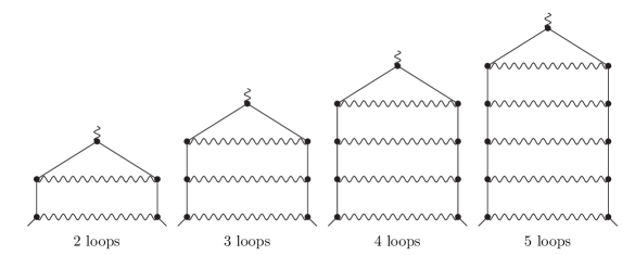
Figure 6: Ladder Feynman graphs.

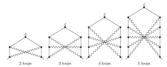
Figure 7: Fully crossed ladder Feynman graphs.

We also have evaluated the individual contributions of the ladder graphs (FIG. 6) and the fully crossed ladder graphs (FIG. 7) up to 5 loops for testing the method and for comparing with the known values. The size of C++ generated code is 2.4 MB for the 5-loop ladder graph and 10 MB for the 5-loop fully crossed ladder graph. The corresponding sizes of the compiled code are 6.2 MB and 24 MB. The contributions of the ladder graphs that are obtained by the presented method are the same as the contributions that are obtained by the standard subtractive on-shell renormalization. This fact can be proved by simple algebraic transformations, see the Section 3 of  [22]. The fully crossed ladder graphs don’t contain divergent subgraphs. Thus, the contributions of the fully crossed ladder graphs don’t depend on the kind of a subtraction procedure. These graphs are a direct test for Monte Carlo integration. The results for the ladder graphs and for the fully crossed ladder graphs are provided in Table LABEL:table_ladder and Table LABEL:table_cross respectively. Here, $\triangle_{\text{prec}}$ is the contribution of the points for which the machine 64-bit precision was not enough. The results for 4-loop and 5-loop fully crossed ladder graphs are new. The dependence of the precision of that 5-loop calculations on number of Monte Carlo samples is shown in Tables LABEL:table_ladder_nsamples, LABEL:table_cross_nsamples (by Diff. we mean the difference between the obtained value and the analytical one from  [46]).

[pos=H,label=table_total, caption=Numerical results ($1\sigma$ limits) for $A_{1}^{(2n)}{[\text{no lepton loops}]}$ and comparison with known analytical values.]cccccccc$N_{l}$ Val. An.val. Ref. $N_{\text{call}}$ $N_{\text{prec}}$ $\sigma_{\uparrow}/\sigma_{\downarrow}$ comp.
2 $-0.34416(10)$ $-0.344167$  [7, 45] $95\cdot 10^{7}$ $10116$ $1.002$ A,6.5h
3 $0.9019(55)$ $0.90437$  [15, 16, 17, 18, 20, 9] $43\cdot 10^{7}$ $60466$ $1.044$ A,24h
4 $-2.34(17)$ $-2.1769$  [21] $10^{9}$ $68\cdot 10^{4}$ $1.17$ B,16d

[pos=H,label=table_4loop,caption=Contributions ($1\sigma$ limits) of the families from FIG. 5 to $A_{1}^{(8)}{[\text{no lepton loops}]}$.]cccccccc # value $N_{\text{call}}$ $\sigma_{\uparrow}/\sigma_{\downarrow}$ # value $N_{\text{call}}$ $\sigma_{\uparrow}/\sigma_{\downarrow}$
$M_{01}$ $-1.198(30)$ $30\cdot 10^{6}$ 1.20 $M_{25}$ $-1.266(14)$ $87\cdot 10^{5}$ 1.30
$M_{02}$ $-1.689(40)$ $47\cdot 10^{6}$ 1.19 $M_{26}$ $-1.598(34)$ $36\cdot 10^{6}$ 1.18
$M_{03}$ $-2.537(35)$ $41\cdot 10^{6}$ 1.15 $M_{27}$ $-0.246(20)$ $16\cdot 10^{6}$ 1.17
$M_{04}$ $6.473(48)$ $71\cdot 10^{6}$ 1.14 $M_{28}$ $6.049(43)$ $58\cdot 10^{6}$ 1.13
$M_{05}$ $4.202(17)$ $12\cdot 10^{6}$ 1.18 $M_{29}$ $1.585(19)$ $14\cdot 10^{6}$ 1.20
$M_{06}$ $-0.990(26)$ $24\cdot 10^{6}$ 1.18 $M_{30}$ $-3.057(33)$ $37\cdot 10^{6}$ 1.14
$M_{07}$ $-2.170(26)$ $23\cdot 10^{6}$ 1.25 $M_{31}$ $0.8248(76)$ $54\cdot 10^{5}$ 1.20
$M_{08}$ $-5.282(42)$ $56\cdot 10^{6}$ 1.16 $M_{32}$ $-0.6672(76)$ $52\cdot 10^{5}$ 1.22
$M_{09}$ $-1.112(27)$ $26\cdot 10^{6}$ 1.15 $M_{33}$ $-0.7301(49)$ $39\cdot 10^{5}$ 1.20
$M_{10}$ $1.845(37)$ $41\cdot 10^{6}$ 1.15 $M_{34}$ $1.084(11)$ $74\cdot 10^{5}$ 1.19
$M_{11}$ $3.244(31)$ $31\cdot 10^{6}$ 1.18 $M_{35}$ $1.859(11)$ $70\cdot 10^{5}$ 1.20
$M_{12}$ $-3.633(36)$ $40\cdot 10^{6}$ 1.14 $M_{36}$ $-1.619(15)$ $10^{7}$ 1.30
$M_{13}$ $-4.337(17)$ $13\cdot 10^{6}$ 1.15 $M_{37}$ $0.9384(54)$ $42\cdot 10^{5}$ 1.22
$M_{14}$ $0.580(29)$ $26\cdot 10^{6}$ 1.23 $M_{38}$ $-4.209(14)$ $93\cdot 10^{5}$ 1.23
$M_{15}$ $0.308(28)$ $27\cdot 10^{6}$ 1.21 $M_{39}$ $-1.982(14)$ $98\cdot 10^{5}$ 1.32
$M_{16}$ $7.507(44)$ $64\cdot 10^{6}$ 1.14 $M_{40}$ $1.548(24)$ $18\cdot 10^{6}$ 1.29
$M_{17}$ $2.895(27)$ $26\cdot 10^{6}$ 1.12 $M_{41}$ $-1.892(19)$ $15\cdot 10^{6}$ 1.20
$M_{18}$ $-4.827(36)$ $42\cdot 10^{6}$ 1.14 $M_{42}$ $2.262(23)$ $20\cdot 10^{6}$ 1.19
$M_{19}$ $0.4035(65)$ $47\cdot 10^{5}$ 1.19 $M_{43}$ $-1.1308(89)$ $57\cdot 10^{5}$ 1.21
$M_{20}$ $2.219(13)$ $86\cdot 10^{5}$ 1.18 $M_{44}$ $2.312(17)$ $13\cdot 10^{6}$ 1.22
$M_{21}$ $0.6548(55)$ $41\cdot 10^{5}$ 1.22 $M_{45}$ $2.109(20)$ $16\cdot 10^{6}$ 1.19
$M_{22}$ $-1.721(16)$ $11\cdot 10^{6}$ 1.21 $M_{46}$ $-0.049(15)$ $10^{7}$ 1.23
$M_{23}$ $-3.150(15)$ $10^{7}$ 1.19 $M_{47}$ $-2.113(21)$ $17\cdot 10^{6}$ 1.19
$M_{24}$ $-0.035(19)$ $15\cdot 10^{6}$ 1.21        

[pos=H,label=table_ladder,caption=Numerical results ($1\sigma$ limits) for the ladder Feynman graphs up to 5 loops and comparison with known analytical values.]ccccccccc$N_{\text{l}}$ Val. An.val. Ref. $N_{\text{call}}$ $N_{\text{prec}}$ $\triangle_{\text{prec}}$ $\sigma_{\uparrow}/\sigma_{\downarrow}$ comp.
2 $0.777440(67)$ $0.777478$  [7, 46] $62\cdot 10^{7}$ $3160$ $0.00005$ $1.001$ A,3h
3 $1.79052(37)$ $1.790278$  [17, 46] $68\cdot 10^{7}$ $15664$ $0.0011$ $1.01$ A,11h
4 $4.3035(39)$ $4.29765$  [46] $39\cdot 10^{7}$ $18997$ $0.018$ $1.08$ A,24h
5 $11.681(46)$ $11.6592$  [46] $4\cdot 10^{8}$ $30652$ $0.25$ $1.32$ A,7.5d

[pos=H,label=table_cross,caption=Numerical results ($1\sigma$ limits) for the fully crossed ladder Feynman graphs up to 5 loops and comparison with known analytical values.]ccccccccc$N_{\text{l}}$ Val. An.val. Ref. $N_{\text{call}}$ $N_{\text{prec}}$ $\triangle_{\text{prec}}$ $\sigma_{\uparrow}/\sigma_{\downarrow}$ comp.
2 $-0.467666(49)$ $-0.467645$  [7] $61\cdot 10^{7}$ $169$ $-4\cdot 10^{-7}$ $1.003$ A,2.5h
3 $-0.026810(47)$ $-0.026800$  [9] $56\cdot 10^{7}$ $16370$ $-5\cdot 10^{-5}$ $1.008$ A,10h
4 $0.29685(21)$ - - $14\cdot 10^{7}$ $25009$ $0.0014$ $1.057$ A,26h
5 $-0.6427(21)$ - - $25\cdot 10^{6}$ $14033$ $-0.018$ $1.228$ A,2.5d

[pos=H,label=table_ladder_nsamples,caption=Dependence of the 5-loop ladder graph precision on $N_{\text{call}}$.]cccccc$N_{\text{call}}$ Val. $\sigma_{\uparrow}$ $\sigma_{\downarrow}$ Diff. $\sigma_{\uparrow}/\sigma_{\downarrow}$
$10^{4}$ $5.02$ $37.4$ $1.85$ $-6.64$ $20.2$
$4\cdot 10^{4}$ $5.79$ $2.21$ $1.2$ $-5.87$ $1.84$
$25\cdot 10^{4}$ $9.2$ $1.28$ $0.7$ $-2.45$ $1.82$
$10^{6}$ $10.42$ $0.64$ $0.42$ $-1.24$ $1.51$
$4\cdot 10^{6}$ $10.67$ $0.33$ $0.23$ $-0.98$ $1.45$
$25\cdot 10^{6}$ $11.236$ $0.167$ $0.112$ $-0.424$ $1.49$
$10^{8}$ $11.621$ $0.089$ $0.064$ $-0.038$ $1.38$
$4\cdot 10^{8}$ $11.6816$ $0.046$ $0.0349$ $0.0224$ $1.32$

[pos=H,label=table_cross_nsamples,caption=Dependence of the 5-loop fully crossed ladder graph $\sigma$ on $N_{\text{call}}$.]ccccc$N_{\text{call}}$ Val. $\sigma_{\uparrow}$ $\sigma_{\downarrow}$ $\sigma_{\uparrow}/\sigma_{\downarrow}$
$10^{4}$ $-0.664$ $0.267$ $0.083$ $3.2$
$4\cdot 10^{4}$ $-0.619$ $0.054$ $0.027$ $2$
$25\cdot 10^{4}$ $-0.6146$ $0.02$ $0.0124$ $1.609$
$10^{6}$ $-0.6318$ $0.0105$ $0.0072$ $1.462$
$4\cdot 10^{6}$ $-0.6369$ $0.00539$ $0.00397$ $1.358$
$25\cdot 10^{6}$ $-0.6427$ $0.00213$ $0.00173$ $1.228$

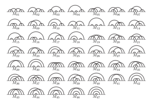
Figure 5: Families of 4-loop Feynman graphs without lepton loops for AMM, the numeration is taken from  [49].

C Comparison with other methods with respect to Monte Carlo convergence speed

Table LABEL:table_mc contains the comparison of the presented method with other ones with respect to Monte Carlo convergence speed. We suppose that $\sigma\sim C/\sqrt{N}$, where $N$ is the number of Monte Carlo samples. Using the value of $C$ we can estimate the convergence speed. The table shows that this method has an advantage over the others. However, we must take into account the following.

• The calculations  [24, 25],  [47],  [48] are not recent. Recent calculations can have improvements in Monte Carlo integration (however, the information about the number of Monte Carlo samples for $A_{1}^{(8)}[\text{no lepton loops}]$ was not provided).

• The information in  [24, 25],  [47],  [48] about the number of samples is very rough.

• The integrands in this calculation and in  [24, 25],  [47],  [48] have a different nature due to the difference in subtraction procedures and in the ways of extracting AMM. It is possible, theoretically, that a slow convergence with respect to number of samples can be compensated by a fast evaluation of integrands.

• In table LABEL:table_mc we don’t take into account the number of samples that were evaluated for residual renormalization in  [24, 25],  [47],  [48]. The presented method doesn’t need residual renormalizations.

• We can have an error underestimation due to a small number of samples. Also, $\sigma\cdot\sqrt{N_{\text{call}}}$ can increase with the rise of $N_{\text{call}}$.

• The error in  [24, 25] was underestimated by about $2.7$ times. The reason is unknown.

• The calculation  [48] was wrong due to an algebraic error  [49].

[pos=H,label=table_mc,caption=Comparison of this method of calculating $A_{1}^{(2n)}{[\text{no lepton loops}]}$ with the others with respect to Monte Carlo convergence speed.]ccccc Calculation Val. $\sigma$ $N_{\text{call}}$ $\sigma\cdot\sqrt{N_{\text{call}}}$
$n=3$, this calculation, 8 integrands $0.9019$ $0.0055$ $43\cdot 10^{7}$ $119.2$
$n=3$,  [24, 25], 8 integrands, RIWIAD $0.74$ $0.06$ $16\cdot 10^{6}$ $240$
$n=3$,  [47], 8 integrands, VEGAS $0.904882$ $0.000347$ $3\cdot 10^{12}$ $601$
$n=4$, this calculation, 47 integrands $-2.34$ $0.17$ $10^{9}$ $5375.9$
$n=4$,  [48], 47 integrands, VEGAS $-1.99306$ $0.00343$ $87\cdot 10^{12}$ $31992.9$

V CONCLUSION

The method for numerical evaluation of $A^{(2n)}_{1}[\text{no lepton loops}]$ was developed. The method is based on the subtraction procedure from  [22] and on the new importance sampling Monte Carlo algorithm. The method has been checked numerically for $n=2,3,4$ on personal computers, the results are in good agreement with the known ones. Also, the contributions of some individual 5-loop graphs were computed. The contributions of the ladder graphs are in good agreement with the known analytical ones ($1.65\sigma$ limits). The obtained contributions of the 4-loop and 5-loop fully crossed ladder graphs are new and can be compared in the future. The method was compared with the other ones with respect to Monte Carlo convergence speed. The new method gives $\sigma$ about 4 times less for $n=3$ and about 6 times less for $n=4$ when the number of samples is fixed. This comparison is not quite correct due to different reasons. However, this shows that the method can be used for precise evaluation of $A^{(2n)}_{1}[\text{no lepton loops}]$ for $n=4$ with the help of supercomputers. The question about effectiveness of the method for $n=5$ is still open. Also, the following problems remain open:

• to prove mathematically (or disprove) that the developed subtraction procedure leads to a finite Feynman-parametric integral for all Feynman graphs for any $n$;

• to prove mathematically that the given probability density function leads to a finite variance $V(f,g)$;

• to develop a method of obtaining $\mathrm{Deg}(s)$ for Feynman graphs containing lepton loops.

References

- [1] D. Hanneke, S. Fogwell Hoogerheide, G. Gabrielse, Cavity control of a single-electron quantum cyclotron: Measuring the electron magnetic moment // Physical Review A. — 2011. — V. 83, 052122.
- [2] T. Aoyama, M. Hayakawa, T. Kinoshita, M. Nio, Tenth-Order Electron Anomalous Magnetic Moment – Contribution of Diagrams without Closed Lepton Loops // Physical Review D. — 2015. — V. 91, 033006.
- [3] R. Bouchendira, P. Cladé, S. Guellati-Khélifa, F. Nez, F. Biraben, New Determination of the Fine Structure Constant and Test of the Quantum Electrodynamics // Physical Review Letters. — 2011. — V. 106, 080801.
- [4] P. Mohr, B. Taylor, D. Newell, CODATA recommended values of the fundamental physical constants: 2010* // Reviews of Modern Physics. — 2012. — V.84, 1527.
- [5] J. Schwinger, On Quantum Electrodynamics and the magnetic moment of the electron // Physical Review. — 1948. — V. 73. — 416.
- [6] J. Schwinger, Quantum Electrodynamics, III: the electromagnetic properties of the electron — radiative corrections to scattering // Physical Review. — 1949. — V. 76. — 790.
- [7] A. Petermann, Fourth order magnetic moment of the electron // Helvetica Physica Acta. — 1957. — V. 30. — 407–408.
- [8] C. Sommerfield, Magnetic dipole moment of the electron // Physical Review. — 1957. – N. 107. — 328–329.
- [9] S. Laporta, E. Remiddi, The Analytical value of the electron (g-2) at order in QED // Physical Letters B. — 1996. — V. 379. — 283–291.
- [10] J. Mignaco, E. Remiddi, Fourth-order vacuum polarization contribution to the sixth-order electron magnetic moment // IL Nuovo Cimento. — 1969. — V. LX A, N. 4. — 519–529.
- [11] R. Barbieri, M. Caffo, E. Remiddi, A contribution to sixth-order electron and muon anomalies. – II // Lettere al Nuovo Cimento. — 1972. – V. 5, N. 11. — 769–773.
- [12] D. Billi, M. Caffo, E. Remiddi, A Contribution to the sixth-Order electron and muon Anomalies // Lettere al Nuovo Cimento. — 1972. — V. 4, N. 14. — 657–660.
- [13] R. Barbieri, E. Remiddi, Sixth order electron and muon from second order vacuum polarization insertion // Physics Letters. — 1974. — V. 49B, N. 5. — 468–470.
- [14] R. Barbieri, M. Caffo, E. Remiddi, A contribution to sixth-order electron and muon anomalies – III // Ref.TH.1802-CERN. — 1974.
- [15] M. Levine, R. Roskies, Hyperspherical approach to quantum electrodynamics: sixth-order magnetic moment // Physical Review D. — 1974. — V. 9, N. 2. — 421–429.
- [16] M. Levine, R. Perisho, R. Roskies, Analytic contributions to the factor of the electron // Physical Review D. — 1976. — V. 13, N. 4. — 997–1002.
- [17] R. Barbieri, M. Caffo, E. Remiddi, S. Turrini, D. Oury, The anomalous magnetic moment of the electron in QED: some more sixth order contributions in the dispersive approach // Nuclear Physics B. — 1978. — N. 144. — 329–348.
- [18] M. Levine, E. Remiddi, R. Roskies, Analytic contributions to the factor of the electron in sixth order // Physical Review D. — 1979. — V. 20, N. 8. — 2068–2077.
- [19] S. Laporta, E. Remiddi, The analytic value of the light-light vertex graph contributions to the electron in QED // Physics Letters B. — 1991. — N. 265. — 182–184.
- [20] S. Laporta, The analytical value of the corner-ladder graphs contribution to the electron in QED // Physics Letters B. — 1995. — N. 343. — 421–426.
- [21] S. Laporta, High-precision calculation of the 4-loop contribution to the electron g-2 in QED, arXiv:1704.06996.
- [22] S. Volkov, Subtractive procedure for calculating the anomalous electron magnetic moment in QED and its application for numerical calculation at the three-loop level, J. Exp. Theor. Phys. (2016), V. 122, N. 6, pp. 1008–1031.
- [23] M. Levine, J. Wright, Anomalous magnetic moment of the electron // Physical Review D. — 1973. — V. 8, N. 9. — 3171–3180.
- [24] R. Carroll, Y. Yao, contributions to the anomalous magnetic moment of an electron in the mass-operator formalism // Physics Letters. — 1974. — V. 48B, N. 2. — 125–127.
- [25] R. Carroll, Mass-operator calculation of the electron factor // Physical Review D. — 1975. — V. 12, N. 8. — 2344–2355.
- [26] P. Cvitanović, T. Kinoshita, Sixth-order magnetic moment of the electron // Physical Review D. — 1974. — V. 10, N. 12. — pp. 4007–4031.
- [27] L.Ts. Adzhemyan, M.V. Kompaniets, Journal of Physics: Conference Series V. 523, N. 1, 012049 (2014).
- [28] N.N. Bogoliubov, O.S. Parasiuk // Acta Math. 97, 227 (1957).
- [29] K. Hepp Proof of the Bogoliubov-Parasiuk Theorem on Renormalization // Commun. math. Phys. — 1966. — V.2. — 301–326.
- [30] V.A. Scherbina // Catalogue of Deposited Papers, VINITI, Moscow, 38, 1964 (in Russian).
- [31] O.I. Zavialov, B.M. Stepanov // Yadernaja Fysika (Nuclear Physics) 1, 922, 1965 (in Russian).
- [32] O.I. Zavialov, Renormalized Quantum Field Theory, Springer Science & Business Media, 2012.
- [33] V.A. Smirnov, Renormalization and Asymptotic Expansions, PPH’14 (Progress in Mathematical Physics), Birkhäuser, 2000.
- [34] S. Weinberg, Infrared Photons and Gravitons, Phys. Rev., V. 140, N. 2B, B516 (1965).
- [35] D. Yennie, S. Frautschi, H. Suura, The Infrared Divergence Phenomena and High-Energy Processes, Annals of Physics 13, 379 (1961).
- [36] G. S. Adkins, R. N. Fell, J. Sapirstein, Two-loop renormalization of Feynman gauge QED, Phys. Rev. D, V. 63, 125009 (2001).
- [37] W. Zimmermann, Convergence of Bogoliubov’s Method of Renormalization in Momentum Space // Commun. math. Phys. — 1969. — V. 15. — 208–234.
- [38] F. Rappl, Feynman Diagram Sampling for Quantum Field Theories on the QPACE 2 Supercomputer, Dissertationsreihe der Fakultät für Physik der Universität Regensburg 49, PhD, Universität Regensburg, 2016.
- [39] E. Speer, Analytic Renormalization, J. Math. Phys. 9, 1404 (1968); doi: 10.1063/1.1664729.
- [40] S. A. Anikin, O. I. Zavialov, M. K. Polivanov, Simple proof of the Bogolyubov-Parasyuk theorem, Theoretical and Mathematical Physics, 17:2 (1973), pp. 1082–1088.
- [41] V.B. Berestetskii, E.M. Lifshitz, L.P. Pitaevskii, Quantum Electrodynamics, Butterworth-Heinemann, 1982.
- [42] F. James, Monte Carlo theory and practice, Rep. Prog. Phys., Vol. 43, N. 9, 1980, pp. 1145–1189.
- [43] P. Cvitanović, T. Kinoshita, Feynman-Dyson rules in parametric space // Physical Review D. — 1974. — V. 10, N. 12. — pp. 3978–3991.
- [44] A. Alexandrescu, The D Programming Language, Addison-Wesley Professional, 2010.
- [45] C. Sommerfield, The Magnetic Moment of the Electron, Annals of Physics: 5, 26–57 (1958).
- [46] M. Caffo, S. Turrini, E. Remiddi, High-order radiative corrections to the electron anomaly in QED: A remark on asymptotic behaviour of vacuum polarization insertions and explitic analytic values for the first six ladder graphs, Nuclear Physics B141 (1978) 302–310.
- [47] T. Kinoshita, New Value of the electron anomalous magnetic moment // Physical Review Letters. — 1995. — V. 75, N. 26. — 4728–4731.
- [48] T. Kinoshita, M. Nio, Improved term of the electron anomalous magnetic moment, Physical Review D 73, 013003 (2006).
- [49] T. Aoyama, M. Hayakawa, T. Kinoshita, M. Nio, Revised value of the eighth-order QED contribution to the anomalous magnetic moment of the electron, Physical Review D 77, 053012 (2008).