Tomographic X-ray data of carved cheese

Abstract

This is the documentation of the tomographic X-ray data of a carved cheese slice. Data are available at www.fips.fi/dataset.php, and can be freely used for scientific purposes with appropriate references to them, and to this document in http://arxiv.org/. The data set consists of (1) the X-ray sinogram of a single 2D slice of the cheese slice with three different resolutions and (2) the corresponding measurement matrices modeling the linear operation of the X-ray transform. Each of these sinograms was obtained from a measured 360-projection fan-beam sinogram by down-sampling and taking logarithms. The original (measured) sinogram is also provided in its original form and resolution.

1 Introduction

The main idea behind the project is to create real CT measurement data for testing sparse and limited data tomography algorithms. A sufficiently thin slice of Edam cheese has been carved with CT letters to recover different attenuation coefficients (calcium-containing organic compounds for cheese and air for the carved letters). In particular, the shape of the carved letters makes the target rather challenging for typical sparse and limited angle tomography applications.

A video report of the data collection session is available at https://www.youtube.com/watch?v=omMrkaCxB2E.

2 Contents of the data set

The data set contains the following MATLAB data files:

• DataFull_512x15.mat,

• DataLimited_512x15.mat,

• DataFull_256x15.mat,

• DataLimited_256x15.mat,

• DataFull_128x15.mat,

• DataLimited_128x15.mat,

• FullSizeSinogram.mat and

• GroundTruthReconstruction.mat.

The first two of these files contain CT sinograms and the corresponding measurement matrices with the same resolution but different spanning for the angle of view: the data in files DataFull_512x15.mat lead to reconstructions with resolutions $512\times 512$ with $15$ directions spanning the full $360$ degree circle; the data in files DataLimited_512x15.mat lead to a reconstructions with resolutions $512\times 512$ with $15$ directions spanning a $90$ degree angle of view. Similarly, the data in files DataFull_256x15.mat and DataLimited_256x15.mat (DataFull_128x15.mat and DataLimited_128x15.mat, respectively) lead to reconstructions with resolutions $256\times 256$ ($128\times 128$, respectively) with $15$ directions spanning the full $360$ degree circle and a $90$ degree angle of view, respectively. The data file named FullSizeSinogram.mat includes the original (measured) sinograms of $360$ projections, and GroundTruthReconstruction.mat contains a high-resolution FBP reconstruction computed from the $360$-projection sinogram. Detailed contents of each data can be found below.

DataFull_512x15.mat contains the following variables:

1. Sparse matrix A of size $14835\times 262144$; measurement matrix.

2. Matrix m of size $989\times 15$; sinogram ($15$ projections spanning the full $360$ degree circle).

3. Scalar normA; norm of the matrix A.

DataLimited_512x15.mat contains the following variables:

1. Sparse matrix A of size $14835\times 262144$; measurement matrix.

2. Matrix m of size $989\times 15$; sinogram ($15$ projections spanning the range $1^{\circ}$– $90^{\circ}$, i.e., a limited angle of view).

3. Scalar normA; norm of the matrix A.

DataFull_256x15.mat contains the following variables:

1. Sparse matrix A of size $14835\times 65536$; measurement matrix.

2. Matrix m of size $989\times 15$; sinogram ($15$ projections spanning the full $360$ degree circle).

3. Scalar normA; norm of the matrix A.

DataLimited_256x15.mat contains the following variables:

1. Sparse matrix A of size $14835\times 65536$; measurement matrix.

2. Matrix m of size $989\times 15$; sinogram ($15$ projections spanning the range $1^{\circ}$– $90^{\circ}$, i.e., a limited angle of view).

3. Scalar normA; norm of the matrix A.

DataFull_128x15.mat contains the following variables:

1. Sparse matrix A of size $14835\times 16384$; measurement matrix.

2. Matrix m of size $989\times 15$; sinogram ($15$ projections spanning the full $360$ degree circle).

3. Scalar normA; norm of the matrix A.

DataLimited_128x15.mat contains the following variables:

1. Sparse matrix A of size $14835\times 16384$; measurement matrix.

2. Matrix m of size $989\times 15$; sinogram ($15$ projections spanning the range $1^{\circ}$– $90^{\circ}$, i.e., a limited angle of view).

3. Scalar normA; norm of the matrix A.

FullSizeSinograms.mat contains the following variables:

1. Matrix sinogram15FullView of size $2240\times 15$; original (measured) sinogram of $15$ projections spanning the full $360$ degree circle.

2. Matrix sinogram15LimitedView of size $2240\times 15$; original (measured) sinogram of $15$ projections spanning the range $1^{\circ}$– $90^{\circ}$ (limited angle of view).

3. Matrix sinogram45FullView of size $2240\times 45$; original (measured) sinogram of $45$ projections spanning the full $360$ degree circle.

4. Matrix sinogram45LimitedView of size $2240\times 45$; original (measured) sinogram of $45$ projections spanning the range $1^{\circ}$– $90^{\circ}$ (limited angle of view).

5. Matrix sinogram180FullView of size $2240\times 180$; original (measured) sinogram of $180$ projections spanning the full $360$ degree circle.

6. Matrix sinogram360 of size $2240\times 360$; original (measured) sinogram of $360$ projections.

GroundTruthReconstruction.mat contains the following variables:

1. Matrix FBP360 of size $2000\times 2000$; a high-resolution filtered back-projection reconstruction computed from the larger sinogram of 360 projections of the carved cheese (“ground truth”). See Figure 5.

Also, we provide the user with the MATLAB routine producing the filtered back-projection reconstruction (script file FBPgroundtruthRec.m).

In addition, at www.fips.fi/dataset.php are available data set with 45 projections (spanning both the full 360 degree circle and the range $1^{\circ}$–$90^{\circ}$) and 180 projections (spanning the full 360 degree circle), for the same three resolutions $512\times 512$, $256\times 256$ and $128\times 128$. Similarly to the 15 projections case, the data set names are DataFull_512x45.mat, DataFull_256x45.mat and DataFull_128x45.mat for the 45 projections case spanning the full 360 degree circle, DataLimited_512x45.mat, DataLimited_256x45.mat and DataLimited_128x45.mat for the 45 limited data case (range $1^{\circ}$–$90^{\circ}$), and DataFull_512x180.mat, DataFull_256x180.mat and DataFull_128x180.mat for the 180 projections case spanning the full 360 degree circle. All these data sets contains the measurement matrix A along with its norm normA and the sinogram m.

Remark. The resolutions of the above datasets are designed specifically so that the total variation regularization parameter choice rule published in [2] can be applied easily. Also, the reason to include the norms of the matrices is the following. Some reconstruction methods require that the norm of the system matrix in equation $Ax=m$ is (at most) one. This can be easily enforced like this in MATLAB:

A = A/normA;
m = m/normA;

After these lines of code the equation is equivalent to the original but the norm of the system matrix is one.

Details on the X-ray measurements are described in Section 3 below. The model for the CT problem is

$${\tt A*x=m(:)},$$ (1)

where m(:) denotes the standard vector form of matrix m in MATLAB and x is the reconstruction in vector form. In other words, the reconstruction task is to find a vector x that (approximately) satisfies (1) and possibly also meets some additional regularization requirements. A demonstration of the use of the data is presented in Section 4.

3 X-ray measurements

Figure 1: The custom-made measurement device at University of Helsinki.

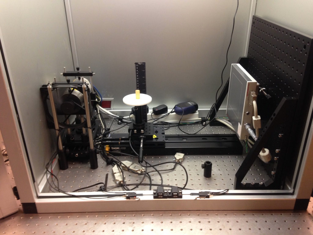
The data in the sinograms are X-ray tomographic (CT) data of a 2D cross-section of the carved cheese measured with a custom-built $\mu$CT device shown in Figure 1.

• The X-ray tube is a model XTF5011 manufactured by Oxford Instruments. This model is no longer sold by Oxford Instruments, although they have newer, similar models available. The tube uses a molybdenum (Z = 42) target.

• The sample manipulator consists of a motorized rotation stage (Thorlabs CR1/M-Z7) mounted onto a motorized horizontal translation stage (Thorlabs LTS300/M), both of which are computer-controlled. The horizontal translation stage allows control of the geometric magnification parameter.

• The flat panel detector is a Hamamatsu Photonics C7942CA-22. The active area of the flat panel detector is 120 mm $\times$ 120 mm. It consists of a $2400\times 2400$ array of 50 $\mu$m pixels. According to the manufacturer the number of active pixels is $2344\times 2240$, which yields an active width of 112 mm. However, the image files actually generated by the camera were $2368\times 2240$ pixels in size.

The measurement setup was designed and assembled in 2015 by Alexander Meaney as a MSc thesis project [1] and recently upgraded (1-3/2017). The setup is illustrated in Figure 1 and the measurement geometry is shown in Figure 3.

A set of $360$ cone-beam projections with resolution $2368\times 2240$ and angular step of one ($1$) degree was measured. The exposure time was $1000$ ms (i.e., one second). The X-ray tube acceleration voltage was $40$ kV and tube current $1$ mA. See Figure 2 for two examples of the resulting projection images.

From the 2D projection images the middle rows corresponding to the central horizontal cross-section of the carved cheese were taken to form a fan-beam sinogram of resolution $2240\times 15$ (variables sinogram15FullView and sinogram15LimitedView in file FullSizeSinograms.mat). These sinograms were further down-sampled by binning and taken logarithms of to obtain the sinograms m in all the files specified in Section 2.

The organization of the pixels in the sinograms and the reconstructions is illustrated in Figure 4.

In addition, a larger set of $360$ projections of the same carved cheese using the same imaging setup and measurement geometry, but with a finer angular step of one $(1)$ degrees, was measured (variable sinogram360 in file FullSizeSinograms.mat). The high-resolution ground truth reconstruction (variable FBP360 in file GroundTruthReconstruction.mat) was computed from this data using filtered back-projection algorithm, see Figure 5.

Figure 2: Left: Experimental setup used for collecting tomographic X-ray data. The detector plane is behind the cheese target with the active area indicated by a white square. The target is attached to a computer-controlled rotator platform. Right: Two examples of the resulting 2D projection images. The fan-beam data in the sinograms consist of the (down-sampled) central rows of the 2D projection images.

Figure 3: Geometry of the measurement setup. Here FOD and FDD denote the focus-to-object distance and the focus-to-detector distance, respectively; the black dot COR is the center-of-rotation. The width of the detector (i.e., the red thick line) is denoted by W. The yellow dot is the X-ray source. To increase clarity, the $x$-axis and $y$-axis in this image are not in scale.

Figure 4: The organization of the pixels in the sinograms m = $[m_{1},m_{2},\ldots,m_{15K}]^{T}$ and the reconstructions x = $[x_{1},x_{2},\ldots,x_{N^{2}}]^{T}$, with $N=128$, $N=256$ or $N=512$. The picture shows the organization for the first projection. After that, in the full angular view case, the target takes a $24$ degree steps counter-clockwise (or, equivalently, the source and detector take a $24$ degree steps clockwise) and the following columns of m are determined in a similar way; in the limited angular view case, the target takes a $6$ degree steps counter-clockwise (or, equivalently, the source and detector take a $6$ degree steps clockwise).

Figure 5: The high-resolution filtered back-projection reconstruction FBP360 of the carved cheese computed from 360 projections.

4 Example of using the data

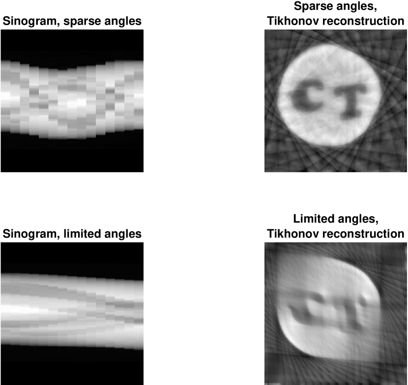
The following MATLAB code demonstrates how to use the data. The code is also provided as the separate MATLAB script file example.m and it assumes the data files (or in this case at least the files DataFull_512x15.mat and DataLimited_512x15.mat) are included in the same directory with the script file. The resulting reconstructed images are reported in Figure 6.

% Load the measurement matrix and the sinogram for the sparse angle case
load DataFull_512x15
N1    = sqrt(size(A,2));
m1    = m;

% Compute a Tikhonov regularized reconstruction using
% conjugate gradient algorithm pcg.m
alpha = 10; % regularization parameter
fun   = @(x) A.’*(A*x)+alpha*x;
b     = A.’*m(:);
x1    = pcg(fun,b);

% Load the measurement matrix and the sinogram for the limited angle case
load DataLimited_512x15
N2    = sqrt(size(A,2));
m2    = m;

% Compute a Tikhonov regularized reconstruction using
% conjugate gradient algorithm pcg.m
alpha = 10; % regularization parameter
fun   = @(x) A.’*(A*x)+alpha*x;
b     = A.’*m(:);
x2    = pcg(fun,b);

% Take a look at the sinograms and the reconstructions
figure
subplot(2,2,1)
imagesc(m1)
colormap gray
axis square
axis off
title(’Sinogram, sparse angles’)
subplot(2,2,3)
imagesc(m2)
colormap gray
axis square
axis off
title(’Sinogram, limited angles’)
subplot(2,2,2)
imagesc(reshape(x1,N1,N1))
colormap gray
axis square
axis off
title({’Sparse angles’; ’Tikhonov reconstruction,’})
subplot(2,2,4)
imagesc(reshape(x2,N2,N2))
colormap gray
axis square
axis off
title({’Limited angles’; ’Tikhonov reconstruction,’})

Figure 6: First row: sinogram and corresponding Tikhonov regularized reconstruction with 15 projections spanning the full 360 degree circle. Second row: sinogram and corresponding Tikhonov regularized reconstruction with 15 projections spanning the range $1^{\circ}$– $90^{\circ}$.

References

- [1] Meaney, A: Design and Construction of an X-ray Computed Tomography Imaging System. MSc Thesis. University of Helsinki, Department of Physics, 2015. http://hdl.handle.net/10138/157237
- [2] Niinimäki K, Lassas M, Hämäläinen K, Kallonen A, Kolehmainen V, Niemi E and Siltanen S, Multi-resolution parameter choice method for total variation regularized tomography. SIAM Journal on Imaging Sciences 9(3) 2016, pp. 938–974.